Three topological phases of
the elliptic Ginibre ensembles with a point charge

Abstract.

We consider the complex and symplectic elliptic Ginibre matrices of size $(c+1)N\times(c+1)N$, conditioned to have a deterministic eigenvalue at $p\in\mathbb{R}$ with multiplicity $cN$. We show that their limiting spectrum is either simply connected, doubly connected, or composed of two disjoint simply connected components. Moreover, denoting by $\tau\in[0,1]$ the non-Hermiticity parameter, we explicitly characterise the regions in the parameter space $(p,c,\tau)$ where each topological type emerges. For cases where the droplet is either simply or doubly connected, we provide an explicit description of the limiting spectrum and the corresponding electrostatic energies. As an application, we derive the asymptotic behaviour of the moments of the characteristic polynomial for elliptic Ginibre matrices in the exponentially varying regime.

1. Introduction and main results

Despite receiving significant attention in recent years, non-Hermitian random matrix theory has historically been less explored than its Hermitian counterpart. This is partly because many key tools used in Hermitian random matrix theory, such as classical orthogonal polynomial theory and group integral techniques, cannot generally be applied to non-Hermitian random matrices. Nonetheless, the past two decades have seen remarkable progress in non-Hermitian random matrix theory, aided by deep connections to other mathematical areas such as the theory of Coulomb gases [95, 58, 86]. We refer the reader to [29] for a recent review of the progress in the field of non-Hermitian random matrices.

Not only is it more challenging, but non-Hermitian random matrix theory has also been found to exhibit more fruitful features than Hermitian random matrix theory. One prominent example is its connection to the topological and conformal geometric properties of the limiting spectral distribution, often referred to as the droplet. For instance, the work of Jancovici et al. [72, 97] in the 1990s introduced the surprising observation that the precise asymptotic behaviour of the free energies is intricately linked to the topological properties of their droplets, as represented by the Euler characteristics (see also [38]). Furthermore, recent studies have revealed that the behaviour of these ensembles depends in a highly non-trivial way on the multiple connectivity or the number of disjoint connected components of droplets [35, 32, 36, 33, 30, 41, 42, 12, 11, 37, 13, 10]. For the critical case involving certain singularities, see [77, 47, 34, 88, 96, 73, 21, 44, 45] and references therein.

This, in turn, calls for explicit derivations of droplets that naturally arise in non-Hermitian random matrices, particularly those with rich topological structure. In this direction, two natural models have been actively investigated in the field, both constructed from the Ginibre matrix [29], a random matrix with independent and identically distributed Gaussian entries, or its variants. The first model adopts an electrostatic perspective. In this approach, a non-trivial point charge is imposed, or equivalently, one considers conditional Ginibre matrices with a prescribed deterministic eigenvalue, see e.g. [17, 35, 77, 51, 20, 75, 21, 82] and references therein. The second model takes a more matrix-theoretic approach, involving the addition of a deterministic matrix to the Ginibre matrix, leading to what are known as deformed Ginibre matrices, see e.g. [47, 39, 55, 87, 88] and references therein.

In this work, we take the first approach and investigate the limiting spectrum of elliptic Ginibre matrices with a point charge. The elliptic Ginibre matrices are indexed by a non-Hermiticity parameter and interpolate between the Ginibre matrices and Gaussian Hermitian random matrices—in our case, the Gaussian unitary and symplectic ensembles. For Ginibre matrices with a point charge, the associated droplet is characterised in the seminal work [17], where it was shown that the droplet is either simply or doubly connected. Our main results in this paper extend these findings, revealing that, when the non-Hermiticity parameter is considered, an additional third phase emerges: a regime where the droplet consists of two connected components. We explicitly derive the regions in the parameter space $(p,c,\tau)$ where each topological type arises. Furthermore, when the droplet is either simply or doubly connected, we provide an explicit description of it as well as its electrostatic energies. As a consequence, we derive the asymptotic behaviours of the moments of the characteristic polynomials of the elliptic Ginibre matrices.

Let us now be more precise in introducing our results. We consider configurations of points $\bm{z}=\{z_{j}\}_{j=1}^{N}$ in the complex plane, with joint probability distribution functions

(1.1) $$d\mathbf{P}_{N}^{\mathbb{C}}(\bm{z}) =\frac{1}{Z_{N}^{\mathbb{C}}(W)}\prod_{1\leq j<k\leq N}|z_{j}-z_{k}|^{2}\prod_{j=1}^{N}e^{-NW(z_{j})}\,\mathrm{d}A(z_{j}),$$

(1.2) $$d\mathbf{P}_{N}^{\mathbb{H}}(\bm{z}) =\frac{1}{Z_{N}^{\mathbb{H}}(W)}\prod_{1\leq j<k\leq N}|z_{j}-z_{k}|^{2}\prod_{1\leq j\leq k\leq N}|z_{j}-\overline{z}_{k}|^{2}\prod_{j=1}^{N}e^{-2NW(z_{j})}\,\mathrm{d}A(z_{j}),$$

where $\,\mathrm{d}A(z)=d^{2}z/\pi$ is the area measure. Here $W:\mathbb{C}\to\mathbb{R}$ is a given external potential, and ${Z_{N}^{\mathbb{C}}(W)}$ and ${Z_{N}^{\mathbb{H}}(W)}$ are the partition functions. The ensembles (1.1) and (1.2) are known as the random normal matrix ensemble and the planar symplectic ensemble, respectively. Moreover, they are equivalent to two-dimensional Coulomb gases at inverse temperature $\beta=2$, with Dirichlet and Neumann boundary conditions, respectively. We also refer to [78, 60, 52] and references therein for a realisation as a fermionic system.

The limiting distribution of the point process $\bm{z}$ can be effectively described using the logarithmic potential theory. Let us briefly recall some basic notions and properties from potential theory, see [89] for a comprehensive source. For a given probability measure $\mu$, the weighted logarithmic energy is given by

(1.3) $$I_{W}(\mu):=\iint_{\mathbb{C}^{2}}\log\frac{1}{|z-w|}\,\mathrm{d}\mu(z)\,\mathrm{d}\mu(w)+\int_{\mathbb{C}}W(z)\,\mathrm{d}\mu(z).$$

It is well known that for a general admissible potential $W$, there exists a unique measure $\mu_{W}$ that minimise $I_{W}$. Furthermore, $\mu_{W}$ is characterised by the variational conditions (Euler-Lagrange equations)

(1.4) $$\int_{\mathbb{C}}\log\frac{1}{|z-w|}\,\mathrm{d}\mu_{W}(w)+\frac{1}{2}W(z)\begin{cases}=C_{W}&z\in\text{supp }\mu_{W},\vskip 3.0pt plus 1.0pt minus 1.0pt\\ \geq C_{W}&z\in\mathbb{C}.\end{cases}$$

Here, $C_{W}$ is called the (modified) Robin’s constant. From the structural point of view, Frostman’s theorem asserts that $\mu_{W}$ is absolutely continuous with respect to the area measure $\,\mathrm{d}A$, and takes the form

(1.5) $$d\mu_{W}=\Delta W\cdot\mathbbm{1}_{S_{W}}\,\mathrm{d}A,\qquad(\Delta:=\partial\bar{\partial}),$$

where $S_{W}$ is a certain compact subset of the complex plane called the droplet.

The equilibrium measure $\mu_{W}$ is closely related to the ensembles (1.1) and (1.2). By standard equilibrium convergence, the empirical measure $\frac{1}{N}\sum_{j=1}^{N}\delta_{z_{j}}$ of the point process $\bm{z}$ converges to the equilibrium measure $\mu_{W}$, see e.g. [95, 40]. In order to see this more intuitively, notice that the Gibbs measures (1.1) and (1.2) are proportional to $\exp(-{\rm{H}}_{N}^{\mathbb{C}}(\bm{z}))$ and $\exp(-{\rm{H}}_{N}^{\mathbb{H}}(\bm{z}))$, where the Hamiltonians are given by

(1.6) $${\rm{H}}_{N}^{\mathbb{C}}(\bm{z}) =\sum_{1\leq j<k\leq N}\log\frac{1}{|z_{j}-z_{k}|^{2}}+N\sum_{j=1}^{N}W(z_{j}),$$

(1.7) $${\rm{H}}_{N}^{\mathbb{H}}(\bm{z}) =\sum_{1\leq j<k\leq N}\log\frac{1}{|z_{j}-z_{k}|^{2}}+\sum_{1\leq j\leq k\leq N}\log\frac{1}{|z_{j}-\overline{z}_{k}|^{2}}+2N\sum_{j=1}^{N}W(z_{j}).$$

Thus one can see that $I_{W}$ in (1.3) corresponds to the continuum limit of these Hamiltonians, after taking proper normalisations. Here, it has been assumed that $W(z)=W(\overline{z})$ for the second case. From the equilibrium convergence, when investigating the macroscopic distribution of the Coulomb gas ensembles, one of the key tasks is to solve the equilibrium measure problem. That is, for a given potential $W$, one aims to determine the associated equilibrium measure $\mu_{W}$. This constitutes a particular type of inverse problem, and due to the structure in (1.5), the main step in this problem is to identify the droplet $S_{W}$. We refer the reader to [27, 25, 4, 24, 18, 17, 43, 30, 85, 1] and references therein for recent development on the planar equilibrium measure problem.

We now turn to our particular model of interest, the conditional elliptic Ginibre ensembles. In order to introduce this, let us first write $G$ for the Ginibre matrices whose entries are complex or quaternionic Gaussian random variables with mean zero and variance $1/N$. Introducing a non-Hermiticity parameter $\tau\in[0,1]$, the elliptic Ginibre matrices are then defined by

(1.8) $$X_{\tau}:=\frac{\sqrt{1+\tau}}{2}(G+G^{*})+\frac{\sqrt{1-\tau}}{2}(G-G^{*}).$$

Then its eigenvalue distribution follows (1.1) and (1.2) respectively, where the associated potential is given by

(1.9) $$W^{\rm e}(z)=\frac{1}{1-\tau^{2}}\Big{(}|z|^{2}-\tau\operatorname{Re}z^{2}\Big{)}.$$

Furthermore, as $N\to\infty$, the eigenvalues tend to be uniformly distributed within an ellipse

(1.10) $$\mathsf{E}=\Big{\{}(x,y)\in\mathbb{R}^{2}:\Big{(}\frac{x}{1+\tau}\Big{)}^{2}+\Big{(}\frac{y}{1-\tau}\Big{)}^{2}\leq 1\Big{\}},$$

which is often called the elliptic law.

Next, for a given $c\geq 0$, we consider the elliptic Ginibre matrix of size $(c+1)N\times(c+1)N$, conditioned to have deterministic eigenvalue at $p\in\mathbb{R}$ with multiplicity $cN$. Then the remaining $N$ random eigenvalues again follow the distributions (1.1) and (1.2), where the associated external potential is given by

(1.11) $$Q(z)=\frac{1}{1-\tau^{2}}\Big{(}|z|^{2}-\tau\operatorname{Re}z^{2}\Big{)}-2c\log|z-p|.$$

Such a logarithmic singularity is often called the point charge insertion or the Fisher-Hartwig singularity. Furthermore, as will be discussed below this section, it is closely related to the moments of the characteristic polynomials [7]. The way to construct the random matrix model with a logarithmic point charge is also known as the inducing procedure [57].

It follows from (1.5) that the equilibrium measure $\mu_{Q}$ is of the form

(1.12) $$d\mu_{Q}=\frac{1}{1-\tau^{2}}\mathbbm{1}_{S_{Q}}\,\mathrm{d}A.$$

In this paper, we aim to provide the topological characterisation of the droplet $S\equiv S_{Q}$. For this purpose, we distinguish the parameter space of $(p,c,\tau)$ into three distinct regimes.

Definition 1 (Regimes of the parameters $p$, $c$ and $\tau$).

We define the following different regimes, cf. Figure 1.

• (Regime I) The first regime is the most explicit and corresponds to the case where $p$ and $c$ lie within the following ranges:

  (1.13) $$p\leq\min\Big{\{}2\sqrt{\frac{2\tau(1+\tau)}{3+\tau^{2}}},2\sqrt{\frac{\tau(1-\tau-2c\tau)}{1-\tau}}\Big{\}}\quad\text{and}\quad 0\leq c\leq\frac{1-\tau}{2\tau},$$

  or

  (1.14) $$2\sqrt{\frac{2\tau(1+\tau)}{3+\tau^{2}}}\leq p\leq(1+\tau)\sqrt{1+c}-\sqrt{c(1-\tau^{2})}\quad\text{and}\quad 0\leq c\leq\frac{(1-\tau)^{3}}{2\tau(3+\tau^{2})}.$$

• (Regime II) The second regime corresponds to the case where for a given $\tau,$ the other parameters $c$ and $p$ are given in terms of two parameters $a$ and $\kappa$ as

  (1.15) $$c \equiv c(a,\kappa)=\frac{\kappa}{a^{2}}\frac{(1-a^{2})^{2}(1-\tau a^{2})+a^{2}\kappa}{(1-a^{2})^{2}(1-\tau^{2}+2\tau\kappa)-\kappa^{2}},$$

  (1.16) $$p \equiv p(a,\kappa)=\sqrt{\frac{1+\tau}{1-\tau}}\frac{(1-\tau)(1-a^{2})(1+\tau a^{2})-(1-\tau a^{2})\kappa}{a\sqrt{(1-a^{2})^{2}(1-\tau^{2}+2\tau\kappa)-\kappa^{2}}}.$$

  Here, the parameters $a$ and $\kappa$ lie in the range

  (1.17) $$a\in(0,1),\qquad\kappa\in[0,\kappa_{\rm cri}),$$

  where $\kappa_{\rm cri}$ is specified as a unique zero of $H(a,\cdot)$ in (4.29).

• (Regime III) This corresponds to the case where the ranges of $p,c$ and $\tau$ lie outside the above two regimes.

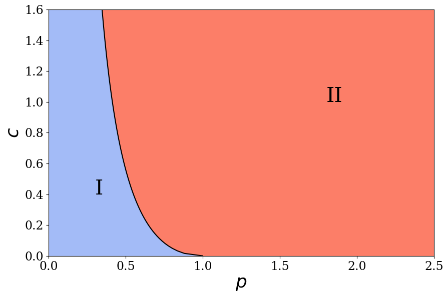
(a) $\tau=0$

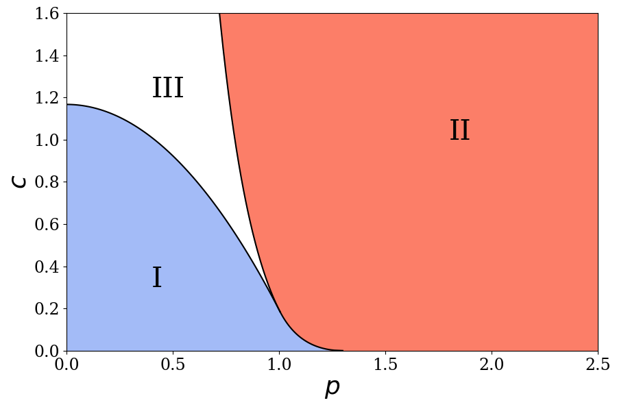
(b) $\tau=0.3$

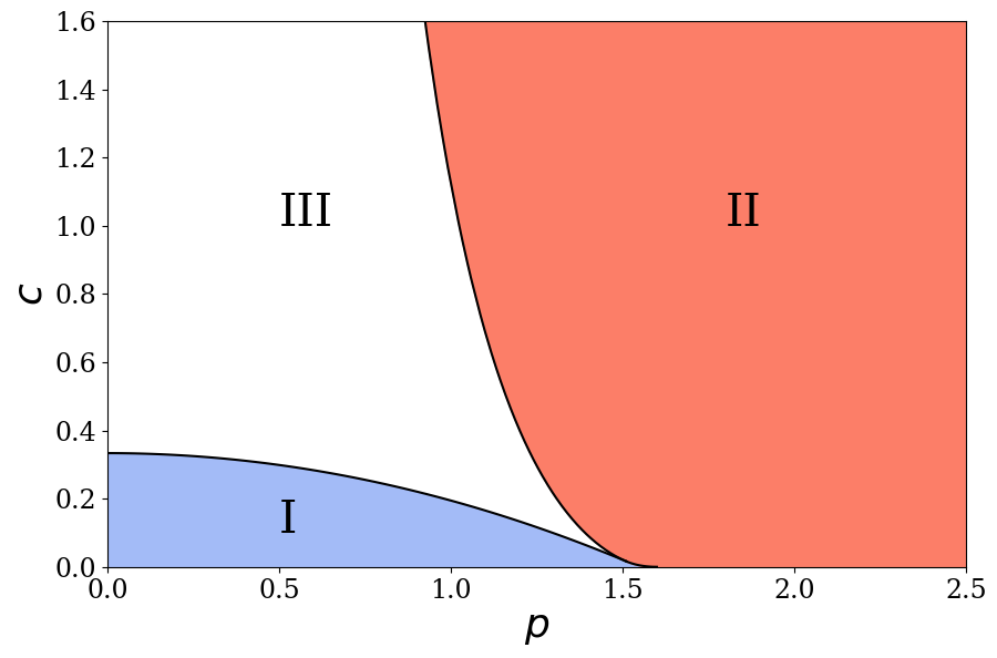
(c) $\tau=0.6$

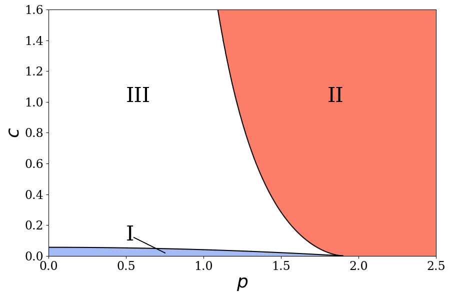
(d) $\tau=0.9$

Figure 1. The plot illustrates Regimes I, II, and III in Definition 1, across various values of $\tau$. Notably, for $\tau=0$, only Regimes I and II are present, while for $p=0$, only Regimes I and III persist, which is consistent with discussions in Remark 1.1.

Our first main result provides the explicit phase characterisation of the droplet.

Theorem 1.1 (Topological characterisation of the droplet).

The droplet $S$ associated with $Q$ defined in (1.11) is either doubly connected, simply connected, or composed of two disjoint simply connected components. More precisely, we have the following.

• The droplet is doubly connected if and only if $(p,c,\tau)$ falls within Regime I.

• The droplet is simply connected if and only if $(p,c,\tau)$ falls within Regime II.

• The droplet consists of two disjoint simply connected components if and only if $(p,c,\tau)$ falls within Regime III.

Remark 1.1 (Phases in extremal cases).

We compare Theorem 1.1 with known results for two extremal cases.

• (The Ginibre case $\tau=0$, cf.[17]). In this case, Regime III reduces to a null set, leaving only Regimes I and II. These two regimes can be determined by the condition

  $$p\leq\sqrt{1+c}-\sqrt{c}\qquad\textup{or}\qquad p>\sqrt{1+c}-\sqrt{c}$$

  for Regimes I and II, respectively. This corresponds to the regimes investigated in [17].

• (The point charge at the origin $p=0$, cf. [27]). In contrast to the previous case, if $p=0$, then Regime II reduces to a null set, leaving only Regimes I and III. These two regimes can be determined by the condition

  $$\tau\leq\frac{1}{1+2c}\qquad\textup{or}\qquad\tau>\frac{1}{1+2c}$$

  for Regimes I and III, respectively. This corresponds to the regimes investigated in [27].

Recall that the weighted logarithmic energy is given by (1.3) and the equilibrium measure $\mu_{Q}$ is of the form (1.12). In cases (i) and (ii) of Theorem 1.1, we further provide an explicit description of the droplets and an evaluation of the logarithmic energies.

Theorem 1.2 (Description of the droplet and electrostatic energies).

We have the following.

• Suppose that $(p,c,\tau)$ falls within Regime I. Then the droplet is given by

  (1.18) $$S=\bigg{\{}(x,y)\in\mathbb{R}^{2}:\Big{(}\frac{x}{1+\tau}\Big{)}^{2}+\Big{(}\frac{y}{1-\tau}\Big{)}^{2}\leq 1+c\,,\,(x-p)^{2}+y^{2}\geq c(1-\tau^{2})\bigg{\}}.$$

  Furthermore, the weighted logarithmic energy is given by $I_{Q}(\mu_{Q})=\mathcal{I}_{\rm d}(p,c,\tau)$, where

  (1.19) $$\mathcal{I}_{\rm d}(p,c,\tau):=\frac{3}{4}+\frac{3c}{2}+\frac{c^{2}}{2}\log\Big{(}c(1-\tau^{2})\Big{)}-\frac{(1+c)^{2}}{2}\log(1+c)-\frac{c\,p^{2}}{1+\tau}.$$

• Suppose that $(p,c,\tau)$ falls within Regime II. Then the droplet is given by the closure of the interior of the real-analytic Jordan curve formed by the image of the unit circle under the rational map

  (1.20) $$f(z)=R\Big{(}z+\frac{\tau}{z}-\frac{\kappa}{z-a}-\frac{\kappa}{a(1-\tau)}\Big{)},$$

  where $R>0$, $a\in(0,1)$, and $\kappa\in[0,\kappa_{\rm cri})$. Here, $(R,a,\kappa)$ is a solution to the coupled algebraic equations

  (1.21) $$1 =\frac{R^{2}}{1-\tau^{2}}\Big{(}1-\tau^{2}+2\tau\kappa-\frac{\kappa^{2}}{(1-a^{2})^{2}}\Big{)},$$

  (1.22) $$c =\frac{R^{2}\kappa}{1-\tau^{2}}\Big{(}\frac{1-\tau a^{2}}{a^{2}}+\frac{\kappa}{(1-a^{2})^{2}}\Big{)},$$

  (1.23) $$p =\frac{R}{a}\Big{(}1+\tau a^{2}-\frac{1-\tau a^{2}}{1-\tau}\frac{\kappa}{1-a^{2}}\Big{)}.$$

  Furthermore, the weighted logarithmic energy is given by $I_{Q}(\mu_{Q})=\mathcal{I}_{\rm s}(p,c,\tau)$, where

  (1.24) $$\begin{split}\mathcal{I}_{\rm s}(p,c,\tau)&=\frac{3}{4}+\frac{3c}{2}-\frac{cp^{2}}{1+\tau}+\frac{R^{3}\kappa p(2-3a^{2}-3\tau a^{2}+2\tau a^{4})}{2(1-\tau^{2})^{2}a^{3}}\Big{(}1-\tau-\frac{2-3a^{2}+3\tau a^{2}-2\tau a^{4}}{2-3a^{2}-3\tau a^{2}+2\tau a^{4}}\frac{\kappa}{1-a^{2}}\Big{)}\\ &\quad+2c(1+c)\log a+c^{2}\log\Big{(}\frac{c(1-\tau^{2})(1-a^{2})}{R\kappa}\Big{)}-(1+c)^{2}\log R.\end{split}$$

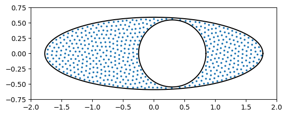
(a) $p=0.3$

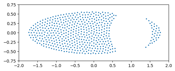
(b) $p=1.0$

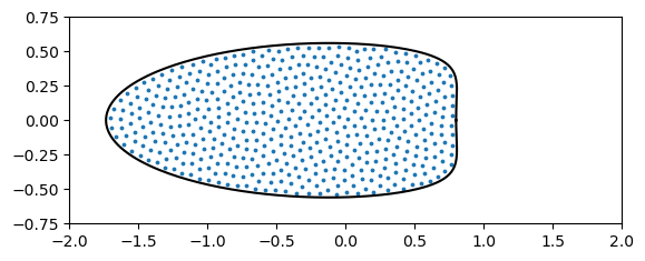
(c) $p=1.5$

Figure 2. The plots illustrate the configurations of Fekete points associated with the Hamiltonian (1.6), with parameters $c=0.4$, $\tau=0.5$, and $N=500$. Regime I corresponds to $p<\sqrt{2/5}\approx 0.63$, while Regime III approximately corresponds to $p>1.12$. In (A) and (C), the black solid lines represent the boundaries of the droplets as determined in Theorem 1.2.

We refer to Figure 2 for numerical verifications of the explicit shape of the droplet, cf. Remark 1.2. Additionally, the graphs of the energies (1.19) and (1.24) are presented in Figure 3.

As previously mentioned, Theorem 1.2 on the description of the droplets extends the findings of [17, Section 2] for the $\tau=0$ case, as well as those of [27, Section 2.1] for the $p=0$ case (see Remark 1.3). Furthermore, Theorem 1.2 on the evaluation of the energies generalises the results in [35, Proposition 2.4] for the $\tau=0$ case. In both extremal cases, the doubly connected regime (Regime I) is referred to as the post-critical regime, while the simply connected regime (Regime II) for $\tau=0$ or the two-component regime (Regime III) for $p=0$ is referred to as the pre-critical regime.

We also note that Regime I in Definition 1 corresponds to the case where, in the description of the droplet (1.18), the outer ellipse does not intersect the inner circle. On the other hand, Proposition 4.1 establishes that in Regime II, the rational map (1.20) is univalent and defines a conformal mapping from the exterior of the unit disc onto the exterior of the droplet.

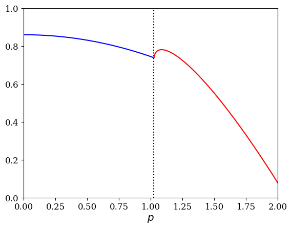
(a) $c=0.15$

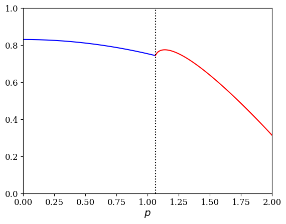
(b) $c=0.1$

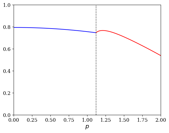
(c) $c=0.05$

Figure 3. The plots display the graphs $p\mapsto I_{Q}(\mu_{Q})$, given by (1.19) and (1.24), for different values of $c$ with $\tau=0.3$. The vertical dotted line indicates the critical value between Regimes I and II.

Remark 1.2 (Fekete points and numerics).

The discrete counterpart of the equilibrium measure is known as the Fekete point distribution, see e.g. [9] and references therein. More precisely, we consider a configuration of points that minimises the Hamiltonians (1.6) and (1.7). These configurations can be interpreted as the low-temperature ($\beta=\infty$) limit of the Coulomb gas ensembles. Since the macroscopic distribution of the Coulomb gas does not depend on the value of fixed $\beta>0$, the Fekete point configuration can be used to numerically observe the shape of the droplet. We also refer to [15] for the $\beta$-ensembles with a flat equilibrium measure.

Remark 1.3 (The extremal $\tau=0$ case).

For the case $\tau=0$, the rational map (1.20) simplifies, as the simple pole at the origin degenerates. Furthermore, the algebraic equations (1.21), (1.22), and (1.22) can be solved more explicitly, leading to the expressions

(1.25) $$R|_{\tau=0}=\frac{1+p^{2}a^{2}}{2pa},\qquad\kappa|_{\tau=0}=\frac{(1-a^{2})(1-p^{2}a^{2})}{1+p^{2}a^{2}}.$$

Here, $a$ satisfies $f(1/a)=p$ and $a^{2}=x$ is given as a unique solution to the cubic equation

(1.26) $$x^{3}-\Big{(}\frac{p^{2}+4c+2}{2p^{2}}\Big{)}x^{2}+\frac{1}{2p^{4}}=0$$

such that $0<a<1$ and $\kappa>0.$ Furthermore, as an immediate consequence of (1.24), for the extremal case $\tau=0$, it follows that

(1.27) $$\begin{split}\mathcal{I}_{\rm s}(p,c,\tau)\Big{|}_{\tau=0}&=\frac{3}{4}+\frac{3c}{2}-cp^{2}+\frac{R^{3}\kappa p}{2a^{3}}(2-3a^{2})\frac{1-a^{2}-\kappa}{1-a^{2}}\\ &\quad+2c(1+c)\log a+c^{2}\log c-c^{2}\log\frac{R\kappa}{(1-a^{2})}-(1+c)^{2}\log R.\end{split}$$

Using (1.25) and (1.26), one can check that this formula is consistent with that derived in [35, Proposition 2.1].

Remark 1.4 (Further phases in the general case).

While some of our results, such as Theorem 1.2 (i), can be naturally extended with minimal additional effort, our focus on the case $p\in\mathbb{R}$ is primarily to make the phase diagram as explicit as possible. Another reason for this focus is that, when considering (1.2), the potential must be symmetric with respect to the real axis. Consequently, for the symplectic ensemble, it is not meaningful to consider only a single point $p\notin\mathbb{R}$. On the other hand, if one considers more point charges at various points, then further phases can arise. The case with multiple point charges have also been studied in the literature including [75, 84, 20, 83].

Remark 1.5 (Critical phases at intersections of different regimes).

There exist various critical regimes at intersections of different regimes. Let us summarise their geometric descriptions.

• The intersection of Regimes I and II is the case where, in (1.18), the outer ellipse meets the inner circle tangentially at the rightmost edge, see Figure 4 (A).

• The intersection of Regimes I and III occurs when, in (1.18), the outer ellipse meets the inner circle tangentially at two conjugate points in the upper and lower half-planes, see Figure 4 (B).

• The intersection of Regimes II and III is less intuitive compared to the previous two cases. At criticality, this corresponds to the emergence of a new archipelago. In Hermitian random matrix theory, the analogous phenomenon has been studied under the name of the birth of a cut, see e.g. [3, 22, 48, 56].

• The “most” critical case is the triple point where all three regimes intersect. For the generic case with $0<\tau<1$ and $p>0$, this critical point occurs when

  (1.28) $$c_{\rm tri}=\frac{(1-\tau)^{3}}{2\tau(3+\tau^{2})},\qquad p_{\rm tri}=2\sqrt{\frac{2\tau(1+\tau)}{3+\tau^{2}}}.$$

  In this case, the outer ellipse again meets the inner circle tangentially at the rightmost edge. Additionally, the curvatures of the ellipse and the circle at this point are identical, see Figure 4 (C).

From the perspective of the ensembles (1.1) and (1.2), several interesting features emerge at such criticality. For the complex Ginibre ensemble, where the critical regime occurs at the intersection of Regimes I and II, the local statistics were recently explored in [77]. In this context, the Painlevé II critical asymptotics arise. Such emergence of critical behaviour is consistent with findings in Hermitian random matrix theory at multi-criticality [23, 49, 50], where the global density vanishes at a bulk point with quadratic decay. Furthermore, a recent study [35] demonstrated that, at this critical point, the Tracy-Widom distribution appears in the constant term of the free energy expansion. This contrasts with the regular case, where the zeta-regularised determinant of the Laplacian is believed to arise (cf. [99]).

Such problems in our present model, the elliptic Ginibre ensembles with a point charge, remain widely open. We expect that the local statistics at the critical points arising at the intersections of Regimes I and II, as well as Regimes I and III, correspond to Painlevé II critical asymptotics, thereby being contained in the same universality class introduced in [77]. Similarly, we expect the Tracy-Widom distribution to emerge in the free energy expansions. In addition, perhaps the most intriguing case in our model is the triple point. At this level of criticality, one might expect the asymptotic behaviours to exhibit the critical asymptotics of higher-order multi-criticality. More precisely, it can be expected that the critical asymptotic behaviour of the Hermitian random matrix model, whose global density vanishes at a bulk point with higher (quartic) order decay, may arise. Consequently, one may expect the Painlevé II hierarchy to emerge in this case.

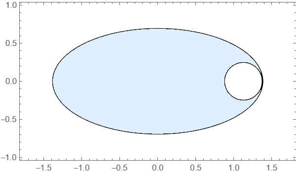
(a) Regimes I & II

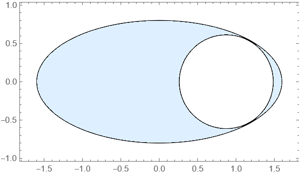
(b) Regimes I & III

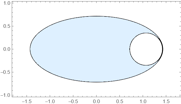
(c) Regimes I, II & III

Figure 4. The plots illustrate various critical phases with $\tau=1/3$. In this case, the triple points (1.28) are given by $c_{\rm tri}=1/7$ and $p_{\rm tri}=2\sqrt{14}/7\approx 1.07$. Plot (A) represents the case $c=1/14<c_{\rm tri}$, where the intersection of Regimes I and II occurs at $p=2\sqrt{7}(\sqrt{30}-1)/21\approx 1.13$. Plot (B) corresponds to the case $c=3/7>c_{\rm tri}$, where $p=4/\sqrt{21}\approx 0.88$. Plot (C) shows the case when $c=c_{\rm tri}$ and $p=p_{\rm tri}$, where the droplet exhibits identical curvatures for the ellipse and circle at the singularity.

Remark 1.6 (Multi-component ensembles in Regime III).

Compared to the Ginibre case when $\tau=0$, one of the interesting features arising in the elliptic case is the emergence of the multi-component ensemble in Regime III. As previously mentioned, the multi-component ensemble has recently gained significant attention, as it exhibits non-trivial additional statistical properties in both the fluctuations [10, 13, 11], represented by the Heine distribution, and various free energy expansions [11, 12, 41, 42], which involve oscillatory asymptotics expressed in terms of the Jacobi theta function. The analogous setup in Hermitian random matrix theory is called the multi-cut regime, where several results are known, see e.g. [46, 26] and references therein.

We also mention that for the case $p=0$, the symmetry of the potential (1.11) with respect to the origin makes it possible to derive the precise shape of the droplets in Regime III. The key idea here is to remove the symmetry, thereby reformulating the problem into an equivalent one where the associated droplet is simply connected. Further details can be found in [27, Remark 1.8].

Remark 1.7 (Phases of the motherbody).

In the study of the point processes (1.1) and (1.2), a natural object of interest is the planar orthogonal polynomials $P_{j}$ associated with the weight $e^{-NW(z)}$. The limiting zero distribution of $P_{j}$ as the degree increases is called the motherbody (or the potential-theoretic skeleton), which is typically a one-dimensional subset of the droplet. The motherbody plays a key role in the asymptotic behaviour of orthogonal polynomials. Clearly, the topology of the motherbody depends strongly on that of the convex hull of the droplet. In addition, the motherbody often exhibits more diverse topological phases. Specifically, within the same topological type of the droplet, further phases of the motherbody may arise. This phenomenon is closely related to the number of critical points of the function $z\mapsto\int_{\mathbb{C}}\log\frac{1}{|z-w|^{2}}\,\mathrm{d}A(w)+W(z)$, which naturally appears in the variational condition (1.4). In our present setting, we expect that in Regime II, where the droplet is simply connected, two distinct phases of the motherbody exist, depending on the number of critical values (cf. Lemma 4.7). For recent developments in this direction, we refer to [75, 25] and references therein.

Remark 1.8 (Equilibrium measure in the Hermitian limit $\tau=1$).

The elliptic Ginibre ensembles provide a natural bridge between Hermitian and non-Hermitian random matrix theories [64, 65, 66]. This characteristic becomes particularly evident in the Hermitian limit $\tau\uparrow 1$, where various intriguing regimes emerge, see, e.g. [5, 6, 8, 28, 74] and references therein for studies on the complex and symplectic elliptic Ginibre ensembles in the almost-Hermitian regime.

We briefly discuss the Hermitian limit of the two-dimensional equilibrium measure. First, by taking the limit $\tau\uparrow 1$ of the potential (1.11), we obtain

(1.29) $$\lim_{\tau\uparrow 1}Q(x+iy)=V(x):=\begin{cases}\displaystyle\frac{x^{2}}{2}-2c\log|x-p|,&\text{if }y=0,\vskip 3.0pt plus 1.0pt minus 1.0pt\\ +\infty&\text{otherwise}.\end{cases}$$

The associated one-dimensional equilibrium measure $\mu_{V}$ is of the form

(1.30) $$\frac{\,\mathrm{d}\mu_{V}(x)}{\,\mathrm{d}x}=\frac{\sqrt{-\prod_{j=1}^{4}(x-\lambda_{j})}}{2\pi|x-p|}\cdot\mathbbm{1}_{[\lambda_{1},\lambda_{2}]\cup[\lambda_{3},\lambda_{4}]}(x),$$

where $\lambda_{1}\leq\lambda_{2}\leq\lambda_{3}\leq\lambda_{4}$ can be computed explicitly, see e.g. [27, Remark 2.3]. In particular, in (1.30), the equilibrium measure is in a multi-cut regime whenever $c>0$. This is consistent with the phase diagram presented in this work, albeit our result strictly focuses on the case $\tau<1$. Namely, for $c>0$, both Regimes I and II degenerate into null sets as $\tau\uparrow 1$, leaving only Regime III.

However, there is an essential difference between the two- and one-dimensional ensembles. Let us provide a heuristic argument based on the electrostatic perspective. To this end, we consider two limits: $c\to\infty$ with fixed $p>0$, or $p\to\infty$ with fixed $c>0$, cf. Remark 4.3. In both cases, the parameters $(p,c,\tau)$ eventually fall within Regime II, meaning that the droplet remains simply connected. Notice that the potential (1.11) implies a confining energy in both the real and imaginary directions, as well as a repulsive energy from the point $p$. Nonetheless, as the strength of the point charge $c$ at $p$ increases, or as the point $p$ where we insert the point charge moves farther away, the particles may detour to form an archipelago that eventually merges into a simply connected droplet. However, this is no longer possible when the particles are strictly confined to the real line, since there is no room for detours in one dimension.

Remark 1.9 (Continuity between Regimes I and II).

It is intuitively clear that there is a smooth transition between different regimes. We shall discuss this aspect via explicit computations between Regimes I and II. For this purpose we take $a\to 1$ limit in Regime II, see [30, Remark 2.6] for a similar discussion. To be more precise, let $\epsilon=\kappa/(1-a^{2})$ be fixed. Then as $a\to 1$, we have

$$c\to\frac{\epsilon^{2}}{1-\tau^{2}-\epsilon^{2}},\qquad p\to(1+\tau-\epsilon)\Big{(}\frac{1-\tau^{2}}{1-\tau^{2}-\epsilon^{2}}\Big{)}^{1/2},\quad 0\leq\epsilon\leq\frac{(1-\tau)^{2}}{1+\tau},$$

which coincides with the parameterisation

(1.31) $$p=(1+\tau)\sqrt{1+c}-\sqrt{c(1-\tau^{2})},\qquad 0\leq c\leq c_{\rm tri}=\frac{(1-\tau)^{3}}{2\tau(3+\tau^{2})}$$

of the boundary of Regime I. In addition to the continuity of the parameter space, one can also observe the continuity of the energies (1.19) and (1.24). To see this, note that from (1.21) and (1.22), we have

$$R^{2}\epsilon^{2}\to c(1-\tau^{2}),\qquad R^{2}\to 1+c,\qquad\kappa\to 0,$$

as $a\to 1$. Therefore, it follows that $\mathcal{I}_{\rm s}\to\mathcal{I}_{\rm d}$ as $a\to 1$, see Figure 3.

We now turn our focus to a more application-oriented perspective on elliptic Ginibre matrices. As previously mentioned, the insertion of a point charge has an equivalent formulation in terms of the moments of characteristic polynomials. For the Ginibre ensembles with $\tau=0$, the moments of the characteristic polynomial $\mathbb{E}|\det(G-z)|^{\gamma}$ have been studied both for fixed $\gamma=O(1)$ [98, 53] and in the exponentially varying regime $\gamma=O(N)$ [35]. These studies have found various applications, such as in the context of Gaussian multiplicative chaos. (See also [62] for a recent study on the convergence of the characteristic polynomial of the complex elliptic Ginibre matrix.)

Corollary 1.3 (Moments of the characteristic polynomials of the elliptic Ginibre matrices).

Let $c>0$ and $\tau\in[0,1)$ be fixed. Let $z\in\mathbb{R}$. Then as $N\to\infty$, we have

(1.32) $$\log\mathbb{E}\Big{[}\,\Big{|}\det(X-z)\Big{|}^{2cN}\Big{]}=\mathcal{K}\,N^{2}+\mathcal{E}_{N},$$

where $\mathcal{K}$ is given as follows.

• If $(p=z,c,\tau)$ falls within Regime I,

  (1.33) $$\mathcal{K}=\frac{c\,z^{2}}{1+\tau}-\frac{3c}{2}+\frac{(1+c)^{2}}{2}\log(1+c)-\frac{c^{2}}{2}\log\Big{(}c(1-\tau^{2})\Big{)}.$$

• If $(p=z,c,\tau)$ falls within Regime II,

  (1.34) $$\begin{split}\mathcal{K}&=\frac{c\,z^{2}}{1+\tau}-\frac{3c}{2}-\frac{R^{3}\kappa(2-3a^{2}-3\tau a^{2}+2\tau a^{4})}{2(1-\tau^{2})^{2}a^{3}}\Big{(}1-\tau-\frac{2-3a^{2}+3\tau a^{2}-2\tau a^{4}}{2-3a^{2}-3\tau a^{2}+2\tau a^{4}}\frac{\kappa}{1-a^{2}}\Big{)}z\\ &\quad-2c(1+c)\log a-c^{2}\log\frac{c(1-\tau^{2})(1-a^{2})}{R\kappa}+(1+c)^{2}\log R,\end{split}$$

  where $(R,a,\kappa)$ is a solution to the coupled algebraic equations (1.21), (1.22) and (1.23) with $p=z$.

Here, the error term is given by

(1.35) $$\mathcal{E}_{N}=\begin{cases}o(N^{1/2+\epsilon})&\textup{for the complex case},\vskip 3.0pt plus 1.0pt minus 1.0pt\\ o(N^{2})&\textup{for the symplectic case},\end{cases}$$

for some $\epsilon>0.$

Note that in terms of the weighted logarithmic energies in Theorem 1.2, we have

(1.36) $$\mathcal{K}=-I_{Q}(\mu_{Q})+\frac{3}{4},$$

where $p$ is identified with $z$. One also notices that the error term in (1.35) becomes significantly more precise in the complex case compared to its symplectic counterparts. This is because, for the complex case, we can utilise recent progress on general Coulomb gases [79, 19, 94, 16], whose symplectic (or Neumann) counterparts are not yet available in the literature. Nonetheless, there are some general conjectures that we can use to formulate a conjecture in our present case. Let us introduce these in a separate remark.

Remark 1.10 (Conjecture on precise error terms).

Due to the general conjecture presented in several works, such as [38, 99, 72, 97] for the complex case and [32] for the symplectic case, we expect that the optimal error term takes the following form.

• For the complex case,

  (1.37) $$\mathcal{E}_{N}=\begin{cases}\frac{1}{12}\log N+O(1)&\textup{in Regime I},\vskip 3.0pt plus 1.0pt minus 1.0pt\\ O(1)&\textup{in Regime II}.\end{cases}$$

• For the symplectic case,

  (1.38) $$\mathcal{E}_{N}=\bigg{(}\int_{\mathsf{E}}\log|z-\bar{z}|\,\,\mathrm{d}A(z)-\int_{S}\log|z-\bar{z}|\,\,\mathrm{d}A(z)\bigg{)}N+\begin{cases}\frac{1}{24}\log N+O(1)&\textup{in Regime I},\vskip 3.0pt plus 1.0pt minus 1.0pt\\ O(1)&\textup{in Regime II}.\end{cases}$$

  Here, $\mathsf{E}$ is given by (1.10).

These precise asymptotic expansions, particularly the coefficients in the $O(\log N)$ terms, reveal a characteristic dependence on the topological properties of the droplet. To be more precise, it is believed that the coefficients of the $\log N$ term in the asymptotic expansion of the free energy is given by

(1.39) $$\frac{1}{2}-\frac{\chi}{12},\qquad\frac{1}{2}-\frac{\chi}{24},$$

for the complex and symplectic case respectively, where $\chi$ is the Euler characteristic of the droplet. Moreover, the $O(1)$ terms are intriguing as well, as they are believed to be intricately linked to certain conformal geometric structures associated with the equilibrium measures.

Remark 1.11 (Duality relation).

For various random matrix ensembles, the moments of characteristic polynomials exhibit duality relations. This implies an identity whereby the averages of characteristic polynomials can be expressed in terms of the averages of certain observables over other random matrices, with the dimension of the latter determined by the exponent of the moments. For a more detailed discussion of this topic, we refer to the recent review [59]. This duality has significant applications in asymptotic analysis, particularly establishing connections between the electrostatic energies of different ensembles, see e.g. [35, 30]. In the case of elliptic Ginibre matrices, the duality relation is derived using Grassmann integration methods, see [92, Proposition 5.1] and [59, Remark 5.1].

Remark 1.12 (Real elliptic Ginibre matrices).

In this work, we focus on the characteristic polynomial of complex and symplectic elliptic Ginibre matrices. On the other hand, the third symmetry class, the real elliptic Ginibre matrices, is also of significant interest and has been actively studied, along with various applications, see e.g. [29, Section 7.9]. A key distinction is that, in the real case, due to the nontrivial probability of having purely real eigenvalues, the eigenvalue distribution no longer forms a one-component plasma system like (1.1) and (1.2) but instead a two-species system. Nonetheless, since the number of real eigenvalues in the strongly non-Hermitian regime (where $\tau<1$ is fixed) is of subdominant order $O(\sqrt{N})$ [54, 61, 31], the macroscopic behaviour (such as the elliptic law) of real elliptic Ginibre matrices remains largely consistent with that of their complex and symplectic counterparts. This, in turn, should also apply to the limiting spectral distribution of conditional elliptic ensembles and the moments of characteristic polynomials. In particular, we expect the same leading-order term, $\mathcal{K}N^{2}$, in (1.32) to appear in the case of real elliptic Ginibre matrices. This gives rise to the exponentially varying counterpart of recent findings [76, 93, 63, 67] for a fixed exponent.

Organisation of the paper

In Section 2, we employ the theory of quadrature domains developed in [81] to establish the first part of Theorem 1.1. Section 3 focuses on the characterisation of the doubly connected domain and the evaluation of its associated energy. Section 4 proceeds in parallel, focusing on the simply connected domain. The final section brings together the results from the preceding sections to conclude the proofs of the main results, Theorems 1.1 and 1.2. Furthermore, Corollary 1.3 is addressed in Subsection 5.2.

Acknowledgements

Sung-Soo Byun was supported by the New Faculty Startup Fund at Seoul National University and by the LAMP Program of the National Research Foundation of Korea (NRF) grant funded by the Ministry of Education (No. RS-2023-00301976). The authors express their gratitude to Peter Forrester, Arno Kuijlaars, Sampad Lahiry, Kohei Noda, Meng Yang and Lun Zhang for their interest and helpful discussions.

2. Quadrature domain and topological characterisation of the droplet

In this section, we recall some known facts about quadrature domains associated with the logarithmic potential, primarily from the work [81] of Lee and Makarov. By employing this theory, we prove the first part of Theorem 1.1, namely, the assertion that the droplet is either doubly connected, simply connected, or composed of two disjoint simply connected components. For a general introduction to quadrature domain theory and related fields, we refer to [70, 81] and references therein.

Recall that a bounded connected open set $\Omega\subset\mathbb{C}$ is called a bounded quadrature domain if it satisfies a quadrature identity: for all integrable analytic functions $f$ on $\Omega$,

(2.1) $$\int_{\Omega}f(\zeta)\,\mathrm{d}A(\zeta)=\sum_{k=1}^{n}c_{k}f^{(m_{k})}(a_{k}),$$

where $n\in\mathbb{Z}_{\geq 0}$ and $(c_{k},m_{k},a_{k})_{k=1}^{n}\subset\mathbb{C}\setminus\{0\}\times\mathbb{Z}_{\geq 0}\times\Omega$. Here, $a_{k}$’s do not necessarily have to be disjoint. For simplicity, we assume that $\partial\Omega$ is a Jordan curve. The quadrature function $r_{\Omega}$ of a quadrature domain $\Omega$ is defined as

(2.2) $$r_{\Omega}(\zeta):=\sum_{k=1}^{n}c_{k}\frac{m_{k}!}{(\zeta-a_{k})^{m_{k}+1}}.$$

Then the quadrature identity (2.1) can be rewritten as

(2.3) $$\int_{\Omega}f(\zeta)\,\mathrm{d}A(\zeta)=\frac{1}{2\pi i}\int_{\partial\Omega}f(\zeta)r_{\Omega}(\zeta)\,\mathrm{d}\zeta.$$

We define the degree of $r_{\Omega}$ as the order of a quadrature domain $\Omega$. Here the degree of a rational function is defined as the maximum of the degree of denominator and numerator in reduced form of the rational function.

The above definition can naturally be extended to unbounded quadrature domains. For this, let $\Omega\subset\hat{\mathbb{C}}$ be a connected open set where $\hat{\mathbb{C}}=\mathbb{C}\cup\{\infty\}$ is the extended complex plane. Assume that $\infty\in\Omega$ and $\partial\Omega$ is a Jordan curve. Then $\Omega$ is an unbounded quadrature domain if it satisfies a quadrature identity (2.1) for all integrable and analytic functions $f$ on $\Omega$ such that $f(\infty)=0$. Observe that if an unbounded quadrature domain $\Omega$ of order $d\geq 0$ does not contain the origin in its closure, inversion with respect to the unit circle conformally maps $\Omega$ to a bounded quadrature domain of order $d+1$. Conversely, a bounded quadrature domain containing the origin can be conformally transformed into an unbounded quadrature domain via circular inversion.

Remark 2.1 (Boundary of a simply connected quadrature domain).

A well-known result due to Aharonov and Shapiro [2] states that a simply connected domain $\Omega$ is a quadrature domain if and only if there exists a rational univalent function $f$ with specific conformal mapping properties:

• if $\Omega$ is a bounded domain, then $f$ conformally maps the unit disc $\mathbb{D}$ onto $\Omega$, with all its poles lying outside the closed unit disc $\bar{\mathbb{D}}$;

• if $\Omega$ is unbounded, then $f$ conformally maps the complement of the closed unit disc, $\bar{\mathbb{D}}^{c}$, onto $\Omega$, with all its poles lying inside $\mathbb{D}$ except for a single simple pole.

Once the quadrature function of a simply connected quadrature domain is given, one can derive explicit rational univalent functions that describe the boundary of the quadrature domain via the so-called conformal mapping method.

Let us provide some examples of bounded and unbounded quadrature domains, which are closely related to our model of interest.

• The open disc $\Omega=\mathbb{D}(p,\rho)$ is a bounded quadrature domain of order 1 with the quadrature function $r_{\Omega}(\zeta)=\rho^{2}/(\zeta-p)$. Indeed, using the mean value property and the Cauchy integral formula, one can observe that

  $$\int_{\mathbb{D}(p,\rho)}f(\zeta)\,\mathrm{d}A(\zeta)=\rho^{2}f(p)=\frac{1}{2\pi i}\int_{|\zeta-p|=\rho}f(\zeta)r_{\Omega}(\zeta)\,\mathrm{d}\zeta.$$

• The exterior of a closed disc, $\Omega=\bar{\mathbb{D}}(p,\rho)^{c}$, can similarly be shown to be an unbounded quadrature domain of order 0, with the quadrature function $r_{\Omega}(\zeta)=\bar{p}$.

• An example of an unbounded quadrature domain of order 1 is the exterior of an ellipse with major and minor axes given by $1\pm\tau$, where $\tau\in[0,1)$. The associated conformal map is the Joukowsky transform $f(z)=z+\tau/z$. By virtue of Remark 2.1, $f$ is a univalent rational function defined on $\bar{\mathbb{D}}^{c}$ with two simple poles at $0$ and $\infty$, one located inside the open unit disc and the other outside the closed unit disc.

Remark 2.2 (Uniqueness problem of quadrature domain).

It is known that if two bounded quadrature domains of order $\leq 2$ share the same quadrature function, they are identical, see [69, Theorem 10 and Corollary 10.1]. In particular, order 1 bounded quadrature domains are precisely the open discs described above.

In contrast, the unbounded analogue of this result is more subtle. For instance, infinitely many order-zero unbounded quadrature domains of the form $\bar{\mathbb{D}}(p,\rho)^{c}$ share the same quadrature function $\bar{p}$. Nevertheless, the uniqueness of unbounded quadrature domains emerges under additional constraints on the area of the domain’s complement. More precisely, it was shown in [81, Theorem 2.1] that if two unbounded quadrature domains have complements of equal area and share the same quadrature function, which is a polynomial of degree at most $2$, then they must be identical.

We now illustrate the connection between quadrature domains and logarithmic potential theory. For this purpose, let us first recall that for a Borel measurable set $\Omega\subset\mathbb{C}$ with compact boundary, the Cauchy transform $C_{\Omega}$ is defined by

(2.4) $$C_{\Omega}(\zeta):=\int_{E}\frac{1}{\zeta-\eta}\,\mathrm{d}A(\eta).$$

Next, assume that $\Omega\subsetneq\hat{\mathbb{C}}$ and $\partial\Omega$ is a Jordan curve such that $\infty\notin\partial\Omega$. If a continuous function $\mathsf{S}_{\Omega}:\bar{\Omega}\to\hat{\mathbb{C}}$ is meromorphic on $\Omega$ and satisfies

(2.5) $$\mathsf{S}_{\Omega}(\zeta)=\bar{\zeta},\qquad\zeta\in\partial\Omega,$$

we call the function $\mathsf{S}\equiv\mathsf{S}_{\Omega}$ as the (one-sided) Schwarz function of $\Omega$. It is clear that if a Schwarz function exists for a domain $\Omega$, then it is unique. The Schwarz function plays a significant role in the theory of quadrature domains. In particular it is well known that $\Omega$ is a quadrature domain if and only if it has a Schwarz function. Moreover, in this case, the following holds:

(2.6) $$\mathsf{S}_{\Omega}(\zeta)=r_{\Omega}(\zeta)+C_{\Omega^{c}}(\zeta),\qquad\zeta\in\bar{\Omega},$$

where $r_{\Omega}$ is the quadrature function (2.2). For a simply connected quadrature domain $\Omega$, we have

(2.7) $$\mathsf{S}_{\Omega}(\zeta)=f(1/F(\zeta)),$$

where $f$ is a rational univalent map associated with $\Omega$ in Remark 2.1, and $F$ is its conformal inverse. For more details, we refer to [81, Lemma 3.1] and references therein.

We now discuss the topological properties of quadrature domains within the framework developed in  [81]. By definition, a Hele-Shaw-type potential $W$ (the potential with constant $\Delta W$) is called an algebraic potential if it is a real valued function defined on an open subset of $\mathbb{C}$, which takes the form

(2.8) $$\frac{1}{t}W(\zeta)=|\zeta|^{2}-H(\zeta),\qquad t>0,$$

where $h:=\partial H$ is a rational function in the variable $\zeta$.

Theorem 2.1 (cf. Theorems 2.3 and 3.3 in [81]).

Let $S\equiv S_{W}$ be the droplet associated with an algebraic potential of the form $W(\zeta)=|\zeta|^{2}-H(\zeta)$. Then $S^{c}$ is a finite union of disjoint quadrature domains $\Omega_{1},\ldots,\Omega_{q}$, and their quadrature functions $r_{1},\ldots,r_{q}$ satisfy

(2.9) $$r_{1}(\zeta)+\ldots+r_{q}(\zeta)=h(\zeta).$$

Let $d$ be the degree of the rational function $h$. Assume that the boundary of $S$ is smooth and consists of disjoint Jordan curves, called the ovals. Let $q_{j}$ be the number of quadrature domains as components of $\hat{\mathbb{C}}\setminus S$ with connectivity $j\geq 1$. Then we have

(2.10) $$\#(\text{ovals})+q_{\text{odd}}+4(q-q_{1})\leq 2d+2.$$

Here, $q=\sum q_{j}$ and $q_{\text{odd}}=\sum q_{2j+1}$.

We also mention that the connectivity bound is indeed sharp [80].

Remark 2.3 (Boundary of a general quadrature domain).

In general, a multiply connected quadrature domain has an “almost” algebraic boundary, meaning that for any quadrature domain $\Omega$ of order $d$, there exists a polynomial $P(\zeta,\eta)$ such that

$$\partial\Omega\subset\{\zeta\in\mathbb{C}:P(\zeta,\bar{\zeta})=0\}.$$

Here, two sets differ by only a finite number of points called special points, see [70, Section 12]. The polynomial $P(\zeta,\eta)$ is symmetric with respect to $\zeta$ and $\eta$, and is of degree $d$ in each variable if $\Omega$ is a bounded quadrature domain, or degree $d+1$ if it is an unbounded quadrature domain. The Schottky double of $\Omega$, a closed Riemann surface constructed by gluing the boundaries of two copies of $\Omega$, can be identified as a real algebraic curve given by $P(\zeta,\mathsf{S}(\zeta))=0$. From the perspective of logarithmic potential theory, the algebraic equation $P(\zeta,\mathsf{S}(\zeta))=0$ is often referred to as the spectral curve, which appears in various contexts, see e.g. [24, 25, 75].

We are now ready to prove the first assertion in Theorem 1.1.

Proof of the first assertion in Theorem 1.1.

Recall that the potential $Q$ is given by (1.11). Let us define

(2.11) $$\mathsf{H}(\zeta):=-\tau\operatorname{Re}\zeta^{2}-2c(1-\tau^{2})\log|\zeta-p|,\qquad\mathsf{h}(\zeta):=\partial\mathsf{H}(\zeta)=\tau\zeta+\frac{c(1-\tau^{2})}{\zeta-p}.$$

The potential (1.11) is clearly an algebraic potential since

(2.12) $$(1-\tau^{2})Q(\zeta)=|\zeta|^{2}-\mathsf{H}(\zeta).$$

Note that the quadrature function $\mathsf{h}$ in (2.11) is of degree 2. By Sakai’s laminarity theorem [91, 90], we can exclude the critical cases and assume that the boundary $\partial S$ is smooth and consists of finitely many Jordan curves, see also [81, Section 5.1]. Then in our present case, the connectivity bound (2.10) reads as

(2.13) $$\#(\text{ovals})+q_{\text{odd}}+4(q-q_{1})\leq 6.$$

Therefore, the possible configurations are as follows:

1. $\#\text{(ovals})=1$, $q_{1}=1$, $q_{j}=0$ for $j\geq 2$;

2. $\#\text{(ovals})=2$, $q_{1}=2$, $q_{j}=0$ for $j\geq 2$;

3. $\#\text{(ovals})=2$, $q_{1}=0$, $q_{2}=1$, $q_{j}=0$ for $j\geq 3$;

4. $\#\text{(ovals)}=3$, $q_{1}=3$, $q_{j}=0$ for $j\geq 2$.

It is evident that (a), (b), (c), and (d) correspond to simply connected droplet, doubly connected droplet, droplet composed of two simply connected components, and triply connected droplet, respectively. These configurations are also presented in [81, Examples $d=0,1,2$ below Theorem 2.3].

We claim that in fact, the droplet $S$ cannot be triply connected. Suppose that the droplet $S$ is triply connected. Then $S^{c}$ consists of an unbounded component $\Omega_{1}$ and bounded components $\Omega_{2},\Omega_{3}$, which are all simply connected quadrature domains. Denote by $r_{1},r_{2}$ and $r_{3}$ the quadrature functions of $\Omega_{1},\Omega_{2}$ and $\Omega_{3}$, respectively. Then it follows from (2.9) and (2.11) that

(2.14) $$r_{1}(\zeta)+r_{2}(\zeta)+r_{3}(\zeta)=\tau\zeta+\frac{c(1-\tau^{2})}{\zeta-p}.$$

Observe that since $\Omega_{2}$ and $\Omega_{3}$ are bounded quadrature domains of order $\geq 1$, both $r_{2}$ and $r_{3}$ must contain distinct poles located in $\Omega_{2}$ and $\Omega_{3}$, respectively. In contrast, $r_{1}$ does not contain a pole in $\Omega_{2}\cup\Omega_{3}$. Therefore, $r_{1}+r_{2}+r_{3}$ must have at least two poles in $\mathbb{C}$. This leads to a contradiction, as the right-hand side of (2.14) contains only a single pole at $p$ in $\mathbb{C}$. Hence, we conclude that the droplet $S$ can only be doubly connected, simply connected, or composed of two disjoint connected components. ∎

Remark 2.4.

It is clear from the proof that for $\tau>0$, the connectivity bound (2.10) does not fully characterise the possible topological types of the droplet, since a triply connected domain may emerge from the connectivity bound, but it does not genuinely occur in practice. In contrast, in the extremal case $\tau=0$, the connectivity bound is sufficient to completely determine the topological types of the droplet. More precisely, when $\tau=0$, the quadrature function has degree 1. Consequently, the possible topological types of the droplet deduced from (2.10) are either simply connected or doubly connected, which is indeed the case, as discussed in Remark 1.3.

3. Doubly connected droplet

In this section, we prove our main results in the regime where the droplet is doubly connected. As one might expect from the simpler description of the droplet in this case, the overall proof and computations are significantly simpler than their counterparts in the simply connected domain, which will be addressed in the next section.

3.1. Description of the droplet

It is convenient to introduce the notations

(3.1) $$E :=\Bigl{\{}(x,y)\in\mathbb{R}^{2}:\Big{(}\frac{x}{1+\tau}\Big{)}^{2}+\Big{(}\frac{y}{1-\tau}\Big{)}^{2}\leq 1+c\Bigl{\}},$$

(3.2) $$D :=\Bigl{\{}(x,y)\in\mathbb{R}^{2}:(x-p)^{2}+y^{2}<c(1-\tau^{2})\Bigl{\}}.$$

Notice that the droplet in (1.18) is the same as $E\cap D^{c}$. Recall that for a given domain $\Omega$, the Schwarz function $\mathsf{S}_{\Omega}$, Cauchy transform $C_{\Omega}$, and quadrature function $r_{\Omega}$ are defined by (2.5), (2.4), and (2.2), respectively.

Let us formulate the following lemma.

Lemma 3.1.

We have

(3.3) $$\mathsf{S}_{E^{c}}(\zeta)=\frac{1+\tau^{2}}{2\tau}\zeta-\frac{1-\tau^{2}}{2\tau}\sqrt{\zeta^{2}-4\tau(1+c)},\qquad\mathsf{S}_{D}(\zeta)=p+\frac{c(1-\tau^{2})}{\zeta-p}$$

and

(3.4) $$C_{E}(\zeta)=\frac{1-\tau^{2}}{2\tau}\Big{(}\zeta-\sqrt{\zeta^{2}-4\tau(1+c)}\Big{)},\qquad C_{D^{c}}(\zeta)=p.$$

Consequently, we have

(3.5) $$r_{E^{c}}(\zeta)=\tau\zeta,\qquad r_{D}(\zeta)=\frac{c(1-\tau^{2})}{\zeta-p}.$$

Proof.

The formulas for the Schwarz functions (3.3) follow directly from straightforward computations using (3.1), (3.2), and (2.5). The evaluation of $C_{E}$ is given by [27, Lemma 2.4]. For the evaluation of $C_{D^{c}}$, notice that for $\zeta\in D$, by using Green’s formula and residue calculus, we have

$$C_{D^{c}}(\zeta) =\int_{D^{c}}\frac{1}{\zeta-\eta}\,\mathrm{d}A(\eta)=-\frac{1}{2\pi i}\int_{\partial D}\frac{\bar{\eta}}{\zeta-\eta}\,\mathrm{d}\eta=-\frac{1}{2\pi i}\int_{\partial D}\frac{\mathsf{S}_{D^{c}}(\eta)}{\zeta-\eta}\,\mathrm{d}\eta=p.$$

Finally, (3.5) follows from (3.3), (3.4) and (2.6). ∎

By Remark 2.2, $D$ is the unique bounded quadrature domain with quadrature function $r_{D}$ of order 1. Similarly, $E^{c}$ is the unique unbounded quadrature domain with quadrature function $r_{E^{c}}$, whose complement has area $\pi(1+c)(1-\tau^{2})$, since $r_{E^{c}}$ is a polynomial of degree less than 2.

Using the previous lemma, we establish the following result. Recall that the potential $Q$ is given by (1.11).

Proposition 3.2.

The droplet $S_{Q}$ is doubly connected if and only if $D\subset E$. In this case, the droplet is given by $E\cap D^{c}$.

Proof.

It has already been established in [27, Proposition 2.1] that if the parameters $(p,c,\tau)$ are chosen such that $D\subset E$, then $S=E\cap D^{c}$. This follows from explicit computations verifying the variational conditions (1.4). Therefore, it suffices to prove that if the droplet is doubly connected, then $D\subset E$.

Suppose the droplet $S$ is doubly connected for given parameters $(p,c,\tau)$. Then $S^{c}$ consists of an unbounded component $\Omega_{1}$ and a bounded component $\Omega_{2}$, both of which are simply connected. By definition, it is obvious that $\Omega_{1}\cap\Omega_{2}=\emptyset$. Since $Q$ is an algebraic potential, by Theorem 2.1, $\Omega_{1}$ and $\Omega_{2}$ are both quadrature domains. Let $r_{1}$ and $r_{2}$ denote the quadrature functions of $\Omega_{1}$ and $\Omega_{2}$, respectively. Then, by (2.9) and (2.11), we have

$$r_{1}(\zeta)+r_{2}(\zeta)=\tau\zeta+\frac{c(1-\tau^{2})}{\zeta-p}.$$

Note that $r_{1}$ and $r_{2}$ are rational functions, with all their poles contained in their respective quadrature domains. In particular, they cannot share the same pole. Additionally, since $\Omega_{2}$ is a bounded quadrature domain, $r_{2}(\zeta)\to 0$ as $\zeta\to\infty$. These conditions imply that

$$r_{1}(\zeta)=\tau\zeta,\qquad r_{2}(\zeta)=\frac{c(1-\tau^{2})}{\zeta-p}.$$

Then, by Lemma 3.1 and the uniqueness property discussed above, it follows that $\Omega_{2}=D$. Furthermore, since the area of $S$ is $\pi(1-\tau^{2})$ (cf. (1.12)), we have

$$\text{area }\Omega_{1}^{c}=\text{area }S+\text{area }\Omega_{2}=\pi(1+c)(1-\tau^{2}).$$

Then, once again, by Lemma 3.1 and the uniqueness property, it follows that $\Omega_{1}=E^{c}$. Therefore by $\Omega_{1}\cap\Omega_{2}=\emptyset$, we conclude that $D\subset E$, which completes the proof. ∎

3.2. Electrostatic energies

In this subsection, we compute the logarithmic energy (1.3). Recall that the Robin’s constant is given by (1.4). Since $\mu_{W}$ is a probability measure, we have

(3.6) $$I_{W}(\mu_{W})=C_{W}+\frac{1}{2}\int_{\mathbb{C}}W(\zeta)\,\mathrm{d}\mu_{W}(\zeta).$$

Lemma 3.3.

Suppose that the droplet $S$ is doubly connected for given parameters $(p,c,\tau)$. Then the Robin’s constant, denoted $C_{\rm d}(p,c,\tau)$, is evaluated as

(3.7) $$C_{\rm d}(p,c,\tau) =\frac{1+c}{2}-\frac{1+c}{2}\log(1+c).$$

Furthermore, we have

(3.8) $$\int_{\mathbb{C}}Q(\zeta)\,\mathrm{d}\mu_{Q}(\zeta) =\frac{1}{2}+2c+c^{2}\log c(1-\tau^{2})-c(1+c)\log(1+c)-\frac{2c\,p^{2}}{1+\tau}.$$

In particular, $\mathcal{I}_{\rm d}(p,c,\tau)$ is given by (1.19).

We note that Lemma 3.3 generalises previous results for $\tau=0$ given in [35, Lemma 4.8, post-critical case]. Additionally, observe that the Robin’s constant does not depend on $p$ and $\tau$ as long as the droplet is doubly connected.

Proof of Lemma 3.3.

By Proposition 3.2 and (1.4), the Robin’s constant can be written as

(3.9) $$C_{\rm d}(p,c,\tau) =\frac{1}{(1-\tau^{2})}\int_{E}\log\frac{1}{|\zeta-\eta|}\,\mathrm{d}A(\eta)-\frac{1}{(1-\tau^{2})}\int_{D}\log\frac{1}{|\zeta-\eta|}\,\mathrm{d}A(\eta)+\frac{1}{2}Q(\zeta),$$

for $\zeta\in S=E\cap D^{c}$. By [27, Lemma 2.4], we have

(3.10) $$\int_{E}\log\frac{1}{|\zeta-\eta|}\,\mathrm{d}A(\eta)=-\frac{1}{2}(|\zeta|^{2}-\tau\operatorname{Re}\zeta^{2})+\int_{E}\log\frac{1}{|\eta|}\,\mathrm{d}A(\eta),\qquad\textup{for }\zeta\in E.$$

On the other hand, by [27, Lemma 2.6], we have

(3.11) $$\int_{D}\log\frac{1}{|\zeta-\eta|}\,\mathrm{d}A(\eta)=-c(1-\tau^{2})\log|\zeta-p|,\qquad\textup{for }\zeta\notin D.$$

Combining all of the above with (1.11), it follows that

(3.12) $$C_{\rm d}(p,c,\tau)=\frac{1}{(1-\tau^{2})}\int_{E}\log\frac{1}{|\eta|}\,\mathrm{d}A(\eta).$$

With the elliptic coordinate $(x,y)=(r(1+\tau)\cos\theta,r(1-\tau)\sin\theta)$, this can be rewritten as

$$C_{\rm d}(p,c,\tau) =-\frac{1}{2\pi}\int_{0}^{2\pi}\int_{0}^{\sqrt{1+c}}\log\Big{(}r^{2}\big{(}(1+\tau)^{2}\cos^{2}\theta+(1-\tau)^{2}\sin^{2}\theta\big{)}\Big{)}r\,\mathrm{d}r\,\mathrm{d}\theta$$

$$=-2\int_{0}^{\sqrt{1+c}}r\log r\,\mathrm{d}r-\frac{1+c}{4\pi}\int_{0}^{2\pi}\log\big{(}(1+\tau)^{2}\cos^{2}\theta+(1-\tau)^{2}\sin^{2}\theta\big{)}\,\mathrm{d}\theta.$$

Then the integral evaluation (see e.g. [68, Eq.(4.226.6)])

$$\int_{0}^{\frac{\pi}{2}}\log(a^{2}\cos^{2}\theta+b^{2}\sin^{2}\theta)\,\mathrm{d}\theta=\pi\log\Big{(}\frac{a+b}{2}\Big{)},\qquad(a,b>0)$$

gives rise to the desired formula (3.7).

Next, we prove (3.8). Note that by (1.11) and (1.5), we have

$$\int_{\mathbb{C}}Q(\zeta)\,\mathrm{d}\mu_{Q}(\zeta) =\frac{1}{(1-\tau^{2})^{2}}\int_{S}|\zeta|^{2}-\tau\operatorname{Re}\zeta^{2}\,\mathrm{d}A(\zeta)+\frac{2c}{1-\tau^{2}}\int_{S}\log\frac{1}{|\zeta-p|}\,\mathrm{d}A(\zeta).$$

By Green’s formula and the change of variables $\zeta=\sqrt{1+c}\,(z+\tau/z)$, we have

(3.13) $$\begin{split}&\quad\int_{E}|\zeta|^{2}-\tau\operatorname{Re}\zeta^{2}\,\mathrm{d}A(\zeta)=\frac{1}{2\pi i}\int_{\partial E}\Big{(}\frac{1}{2}\bar{\zeta}-\tau\zeta\Big{)}|\zeta|^{2}\,\mathrm{d}\zeta\\ &=\frac{(1+c)^{2}}{2\pi i}\int_{\partial\mathbb{D}}\bigg{(}\frac{1}{2}\Big{(}z+\frac{\tau}{z}\Big{)}\Big{(}\frac{1}{z}+\tau z\Big{)}^{2}-\tau\Big{(}z+\frac{\tau}{z}\Big{)}^{2}\Big{(}\frac{1}{z}+\tau z\Big{)}\bigg{)}\Big{(}1-\frac{\tau}{z^{2}}\Big{)}\,\mathrm{d}z=\frac{(1+c)^{2}}{2}(1-\tau^{2})^{2}.\end{split}$$

Here, the last equality follows directly from straightforward residue calculus.

Similarly, with the change of variables $\zeta=p+\sqrt{c(1-\tau^{2})}z$, we have

(3.14) $$\begin{split}\int_{D}|\zeta|^{2}-\tau\operatorname{Re}\zeta^{2}\,\mathrm{d}A(\zeta)=\frac{1}{2\pi i}\int_{\partial D}\Big{(}\frac{1}{2}\bar{\zeta}-\tau\zeta\Big{)}|\zeta|^{2}\,\mathrm{d}\zeta=\Big{(}\frac{c^{2}}{2}+\frac{cp^{2}}{1+\tau}\Big{)}(1-\tau^{2})^{2}.\end{split}$$

On the other hand, by applying (3.10), we have

(3.15) $$\begin{split}\frac{1}{1-\tau^{2}}\int_{S}\log\frac{1}{|\zeta-p|}\,\mathrm{d}A(\zeta)&=-\frac{p^{2}}{2(1+\tau)}+\frac{1}{2}-\frac{1+c}{2}\log(1+c)+\frac{c}{2}\log c(1-\tau^{2}).\end{split}$$

Combining all of the above, we obtain (3.8).

The last assertion immediately follows from (3.7) and (3.8), together with (3.6). ∎

4. Simply connected droplet

In this section, we establish our main results in the regime where the droplet is simply connected.

An effective approach to determining the shape of the droplet is the so-called conformal mapping method. This method relies on an a priori assumption about the topology of the droplet–simple connectedness in our case–and then seeks to characterise a conformal map $f$ that maps $\bar{\mathbb{D}}^{c}$ conformally onto $S^{c}$. The general procedure is as follows: First, we make use of the explicit form of the Schwarz function to extend $f$ analytically to the entire complex plane. Then, by identifying the locations and coefficients of its poles, we establish that $f$ is a rational function via Liouville’s theorem. Indeed, for Hele-Shaw-type potentials, where the density of the equilibrium measure is flat, it is known in general that $f$ is a rational univalent map on $\bar{\mathbb{D}}^{c}$, cf. Remark 2.1. For implementations of this strategy in various models, see [4, 27, 30]. This method is powerful for determining the explicit shape of the droplet; however, once the conformal map is specified, one must still verify the variational conditions (1.4) to justify the a priori assumption about the topology of the droplet.

Previous work in this direction [4, 27, 30] has shown that, although the conformal mapping method requires separate verification of the variational conditions (1.4), it nevertheless yields the correct answer for the droplet. However, this is not entirely the case in our present setting. More precisely, the conformal mapping method provides an ansatz for the rational map but does not fully characterise the droplet, as the range of the parameter $\kappa$ obtained through this method is larger than the true solution, see Figure 5. Consequently, determining the correct range, which is indeed the challenging part, becomes essential when verifying the variational conditions.

Let us be more precise within our current setup. Recall that the rational map $f$ is given by (1.20), with parameters $(R,a,\kappa)$ satisfying the algebraic conditions (1.21), (1.22), and (1.23). Here, it is crucial that $a\in(0,1)$ and $\kappa\in[0,\kappa_{\rm cri})$, where $\kappa_{\rm cri}$ is the unique zero of $H(a,\cdot)$ in (4.29). Beyond $\kappa_{\rm cri}$, there exist additional critical values of $\kappa$ that determine the geometric properties of $f(\partial\mathbb{D})$:

(4.1) $$\kappa_{\rm min}=-(1-\tau)(1-a)^{2},\qquad\kappa_{\rm max}=\frac{(1-\tau a^{2})^{2}}{(1+\tau a^{2})^{2}}(1+\tau)(1-a^{2}).$$

Later, in the proof of Proposition 4.5, we will verify that $\kappa_{\rm cri}\leq\kappa_{\rm max}$. We summarise the key geometric properties of $f(\partial\mathbb{D})$ depending on the values of $\kappa$, along with our overall argument to establish the main results.

• (Univalence condition) In general, the rational map $f$ of the form (1.20) is not univalent on $\bar{\mathbb{D}}^{c}$. However, Proposition 4.1 shows that $f$ is univalent on $\bar{\mathbb{D}}^{c}$ if and only if $\kappa\in[\kappa_{\rm min},\kappa_{\rm max}]$. Furthermore, this condition is equivalent to requiring that $S_{Q}^{c}$ is a quadrature domain. While this step is not essential to completing the proof of our main results, it provides a necessary condition for the range of $\kappa$.

• (A priori droplet condition) Suppose that the droplet $S_{Q}$ is simply connected. Then, using the conformal mapping method introduced above, Proposition 4.2 shows that $S_{Q}$ is enclosed by the rational map $f$ of the form (1.20), where $\kappa\in[0,\kappa_{\rm max}]$. Here, compared to the univalence condition, which requires $\kappa\in[\kappa_{\rm min},\kappa_{\rm max}]$, the range $\kappa\in[\kappa_{\rm min},0)$ is excluded. From a computational perspective, this follows from the fact that $c\geq 0$, which is necessary to ensure the finiteness of the partition functions in (1.1) and (1.2).

• (Variational conditions) As explained above, the previous step is not necessary to fully characterise the droplet, as $\kappa_{\rm cri}$ can be strictly smaller than $\kappa_{\rm max}$. In the final step, we must verify that a genuine droplet arises only when $\kappa\in[0,\kappa_{\rm cri})$. For this purpose, let $K$ be a simply connected domain enclosed by the image of the unit circle under the rational map (1.20), where $\kappa\in[0,\kappa_{\rm max}]$. Then, in Propositions 4.4 and 4.5, we show that the probability measure (cf. Lemma 4.3)

  (4.2) $$\mu_{K}:=\frac{1}{1-\tau^{2}}\mathbbm{1}_{K}\,\mathrm{d}A$$

  satisfies the variational conditions (1.4) if and only if $\kappa\in[0,\kappa_{\rm cri})$.

See Figure 5 for an illustration and summary of this discussion.

Figure 5. The plot illustrates the ranges of $\kappa$ for which different geometric properties of $f(\partial\mathbb{D})$ arise.

We note that (4.2) constitutes a slight abuse of notation, as $\mu_{Q}$ also denotes the equilibrium measure associated with the potential $Q$. However, since $\mu_{Q}$ does not appear elsewhere in this section, we believe no ambiguity should arise.

From the perspective of the phase diagram, the critical value $\kappa_{\rm cri}$ corresponds to the intersection of Regimes II and III, marking the emergence of a new archipelago. See Figure 6 for images of $f(\partial\mathbb{D})$, where different phases can be observed depending on the values of $\kappa$.

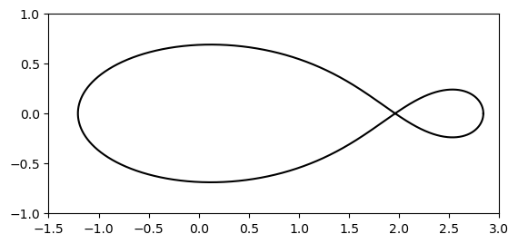
(a) $\kappa=-0.2<\kappa_{\rm min}$

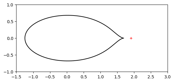
(b) $\kappa=\kappa_{\rm min}=-0.063$

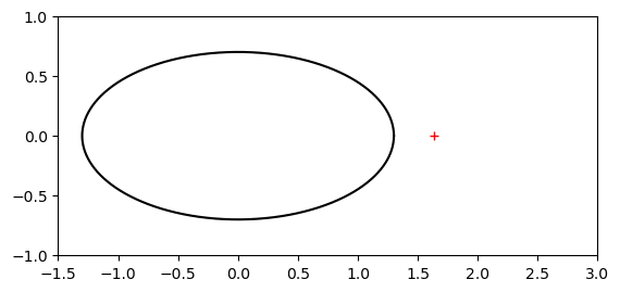
(c) $\kappa=0$

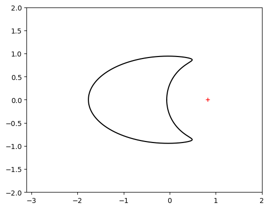
(d) $\kappa=\kappa_{\rm cri}\approx 0.253$

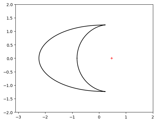
(e) $\kappa=\kappa_{\rm max}\approx 0.367$

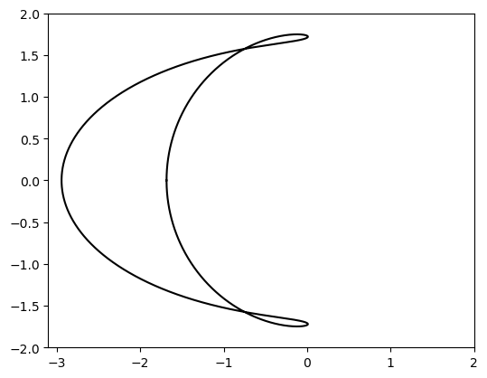
(f) $\kappa=0.45>\kappa_{\rm max}$

Figure 6. The plots show the image of $f(\partial\mathbb{D})$ for $\tau=0.3$ and $a=0.7$, with different values of $\kappa$. The red cross in (B)–(E) indicates the point $p$. It is clear that in (A) and (F), where $\kappa<\kappa_{\rm min}$ or $\kappa>\kappa_{\rm max}$, the rational map $f$ is no longer univalent on $\bar{\mathbb{D}}^{c}$. Plots (B) and (E) illustrate cases where univalence breaks, while plots (C) and (D) correspond to regimes where $f(\partial\mathbb{D})$ forms the boundary of the droplet.

4.1. Univalence criterion and conformal mapping method

In this subsection, we discuss the a priori condition for droplet.

We first state the univalence criterion for the rational function $f$ of the form  (1.20).

Proposition 4.1.

Let $f$ be a rational function of the form (1.20), where $R>0$, $a\in(0,1)$, and $\tau\in[0,1)$. Then, for $\kappa\in\mathbb{R}$, $f$ is univalent on $\bar{\mathbb{D}}^{c}$ if and only if $\kappa\in[\kappa_{\rm min},\kappa_{\rm max}]$.

This proposition is not directly used to prove our main results. Nonetheless, it highlights an interesting feature of the rational map $f$, and we defer the proof of Proposition 4.1 to Appendix A. We note that the proof is based on the Schur-Cohn test.

Next, we formulate the a priori condition for the droplet, which leads to the ansatz for the droplet under the assumption that it is simply connected.

Proposition 4.2.

Suppose the droplet $S$ associated with the potential $Q$ is simply connected. Then, there exists a rational map $f$ of the form (1.20) that conformally maps $\bar{\mathbb{D}}^{c}$ onto $S^{c}$. Here, $(R,a,\kappa)$ satisfy the algebraic equations (1.21), (1.22), and (1.23), where $R>0$, $a\in(0,1)$, and $\kappa\in[0,\kappa_{\rm max}]$.

Before presenting the proof, we first comment on the positivity of the parameter $a$. Intuitively, this may seem clear since the point $p$, where the point charge is inserted, is non-negative, meaning that the droplet leans towards the left half-plane. However, a rigorous proof requires a finer upper bound on $\kappa$, which is more naturally discussed after Proposition 4.5. Therefore, we postpone the proof of $a>0$ to the end of Section 4.2, see Remark 4.1.

Proof of Proposition 4.2.

By Theorem 2.1, $S^{c}$ is a simply connected, unbounded quadrature domain with quadrature function $\mathsf{h}$ given by (2.11). Since $\mathsf{h}$ has a pole at $p$, it follows that $p$ does not belong to $S$. Furthermore, there exists a rational conformal map that conformally maps $\bar{\mathbb{D}}^{c}$ onto $S^{c}$, cf. Remark 2.1. Therefore, there is a unique rational function $f$ such that $f=R\,z+O(1)$ as $z\to\infty$ where $R>0$. We denote by $\mathsf{S}\equiv\mathsf{S}_{S^{c}}$ the Schwarz function of $S^{c}$. Then by (2.6), we have

$$\mathsf{S}(\zeta)=C_{S}(\zeta)+\tau\zeta+\frac{c(1-\tau^{2})}{\zeta-p},\qquad\zeta\in(\operatorname{Int}S)^{c}.$$

Recall here that the Cauchy transform $C_{S}$ is defined by (2.4). Notice here that for $z\in\partial\mathbb{D}$, by (2.5), we have

(4.3) $$f(z)=f(1/\bar{z})=\overline{f(1/z)}=C_{S}(f(1/z))+\tau f(1/z)+\frac{c(1-\tau^{2})}{f(1/z)-p}.$$

Observe that the last expression is meromorphic with respect to $z$ on $\mathbb{D}$, with at most two poles at $z=0$ and $z=a$, where $f(1/a)=p$. Note that such an $a\in\mathbb{D}\setminus\{0\}$ exists uniquely since $f$ conformally maps $\bar{\mathbb{D}}^{c}$ onto $S^{c}$. Moreover, due to the univalence of $f$, these poles are simple. Therefore, the conformal map $f$ is of the form

(4.4) $$f(z)=R\Big{(}z+r_{1}+\frac{r_{2}}{z}+\frac{r_{3}}{z-a}\Big{)},$$

where $r_{1},r_{2},r_{3}\in\mathbb{R}$ and $a\in(-1,0)\cup(0,1)$ by the symmetry of the droplet along the real axis.

Next, we determine the coefficients $r_{1},r_{2}$, and $r_{3}$. Then we verify that the parameters satisfy the algebraic equations (1.21), (1.22), and (1.23). To establish this, we compute the asymptotics of each term in (4.3) as $z\to 0$ and $z\to a$. We first notice from (4.4) that

$$\begin{split}f(z)=\begin{cases}\displaystyle\frac{Rr_{2}}{z}+R\Big{(}r_{1}-\frac{r_{3}}{a^{2}}\Big{)}+R\Big{(}1-\frac{r_{3}}{a^{2}}\Big{)}z+O(z^{2}),&\textup{as }z\to 0,\vskip 3.0pt plus 1.0pt minus 1.0pt\\ \displaystyle\frac{Rr_{3}}{z-a}+O(1),&\textup{as }z\to a.\end{cases}\end{split}$$

Consequently, it follows from straightforward computations that

$$f(1/z) =\begin{cases}\displaystyle\frac{R}{z}+Rr_{1}+R(r_{2}+r_{3})z+O(z^{2}),&\textup{as }z\to 0,\vskip 3.0pt plus 1.0pt minus 1.0pt\\ O(1),&\textup{as }z\to a,\end{cases}$$

$$\frac{1}{f(1/z)-p} =\begin{cases}\displaystyle\frac{z}{R}+O(z^{2}),&\textup{as }z\to 0,\vskip 3.0pt plus 1.0pt minus 1.0pt\\ \displaystyle-\frac{1}{R}\Big{(}\frac{1-\tau a^{2}}{a^{2}}-\frac{r_{3}}{(1-a^{2})^{2}}\Big{)}^{-1}\frac{1}{z-a}+O(1),&\textup{as }z\to a.\end{cases}$$

Note that by definition (2.4), we have

$$C_{S}(\zeta)=\frac{1-\tau^{2}}{\zeta}+O(1/\zeta^{2}),\qquad\zeta\to\infty,$$

where we have used $\text{area }S=\pi(1-\tau^{2})$, cf. (1.12). Then it follows that

$$C_{S}(f(1/z))=\begin{cases}\displaystyle\frac{1-\tau^{2}}{R}z+O(z^{2}),&\textup{as }z\to 0,\vskip 3.0pt plus 1.0pt minus 1.0pt\\ \displaystyle O(1),&\textup{as }z\to a.\end{cases}$$

In consistency with (1.20), let $r_{3}=-\kappa$. Then, by comparing the asymptotic behavior of both sides of (4.3) as $z\to 0$, we obtain

(4.5) $$r_{1}=-\frac{\kappa}{a(1-\tau)},\qquad r_{2}=\tau$$

and

(4.6) $$(1+c)(1-\tau^{2})=R^{2}\Big{(}1-\tau^{2}+\frac{1+\tau a^{2}}{a^{2}}\kappa\Big{)}.$$

Therefore, we have shown that $f$ is of the form (1.20). By comparing the asymptotic behaviour of both sides of (4.3) as $z\to a$, we obtain (1.22). Combining (1.22) and (4.6) leads to (1.21). Finally, the condition $f(1/a)=p$ yields (1.23).

Now we show that $\kappa\in[0,\kappa_{\rm max}]$. Since $f$ is assumed to be univalent on $\bar{\mathbb{D}}^{c}$, Proposition 4.1 ensures that $\kappa\in[\kappa_{\rm min},\kappa_{\rm max}]$. Note that by (1.22) and the requirement $c\geq 0$, we have

$$\kappa\geq 0\quad\text{ or }\quad\kappa\leq-\frac{1-\tau a^{2}}{a^{2}}(1-a^{2})^{2}.$$

On the other hand, by (4.1) and the fact that $\kappa>\kappa_{\min}$, the second range is not possible, which leads to $\kappa\in[0,\kappa_{\rm max}]$. ∎

4.2. Variational conditions

Recall that $K$ is a simply connected domain enclosed by the image of the unit circle under the rational map (1.20), where $\kappa\in[0,\kappa_{\rm max}]$, and that $\mu_{K}$ is given by (4.2). Our goal is to show that the ansatz $\mu_{K}$ is indeed the equilibrium measure associated with the potential $Q$. In other words, we aim to prove that

(4.7) $$K=S\qquad\textup{if }\kappa\in[0,\kappa_{\rm cri}).$$

To establish this, we must exclude the range $\kappa\in[\kappa_{\rm cri},\kappa_{\rm max}]$. As previously mentioned, this follows from verifying the variational conditions (1.4). In Proposition 4.4, we prove that the equality part of (1.4) holds for $\mu_{Q}=\mu_{K}$ for all $\kappa\in[0,\kappa_{\rm max}]$. On the other hand, in Proposition 4.5, we establish that the inequality part of (1.4) holds if and only if $\kappa\in[0,\kappa_{\rm cri})$. By the uniqueness of the equilibrium measure, Propositions 4.4 and 4.5 fully characterise the simply connected case.

Note that the case $\tau=0$ was already addressed in [17] (see also Remark 1.3). Therefore, we focus on the case $\tau\in(0,1)$, which simplifies certain aspects of the presentation.

Throughout this subsection, we assume that $\tau\in(0,1)$, $a\in(0,1)$, and $\kappa\in[0,\kappa_{\rm max}]$, with $c$ and $p$ given by (1.15) and (1.16). We first discuss that $\mu_{K}$ is indeed a probability measure.

Lemma 4.3.

The measure $\mu_{K}$ in (4.2) has a total mass of 1.

Proof.

It suffices to show that the area of $K$ is $\pi(1-\tau^{2})$. By using Green’s formula, we have

$$\frac{\text{area }K}{\pi}=\frac{1}{2\pi i}\int_{\partial K}\bar{\zeta}\,\mathrm{d}\zeta=\frac{1}{2\pi i}\int_{\partial\mathbb{D}}f(1/z)f^{\prime}(z)\,\mathrm{d}z=\underset{z=0}{\textrm{Res}}\Big{[}f(1/z)f^{\prime}(z)\Big{]}+\underset{z=a}{\textrm{Res}}\Big{[}f(1/z)f^{\prime}(z)\Big{]}.$$

Here, residue calculus using (1.20), (1.21), and (1.22) gives that

$$\underset{z=0}{\textrm{Res}}\Big{[}f(1/z)f^{\prime}(z)\Big{]}=(1+c)(1-\tau^{2}),\qquad\underset{z=a}{\textrm{Res}}\Big{[}f(1/z)f^{\prime}(z)\Big{]}=-c(1-\tau^{2}).$$

This completes the proof. ∎

We define $\mathcal{U}_{K}:\mathbb{C}\to(-\infty,\infty]$ by

(4.8) $$\mathcal{U}_{K}(\zeta)=\frac{1}{1-\tau^{2}}\int_{K}\log\frac{1}{|\zeta-\eta|^{2}}\,\mathrm{d}A(\eta)+Q(\zeta).$$

This is the left hand side of (1.4), up to multiplicative constant. Notice that $\mathcal{U}_{K}$ is a continuous function that diverges to infinity as $|\zeta|\to\infty$ and at $\zeta=p$ if $c>0$.

Proposition 4.4.

For $\zeta\in K$, we have $\mathcal{U}_{K}(\zeta)=\ell_{K}$ for some constant $\ell_{K}$.

By Proposition 4.4, we can take

(4.9) $$\ell_{K}=\mathcal{U}_{K}(f(1)).$$

Notice that once $K$ is proven to be the droplet, this value coincides with twice the Robin’s constant.

Proof of Proposition 4.4.

Since $K$ is a simply connected subset of $\mathbb{C}$, it is enough to show that the derivative $\partial_{\zeta}\mathcal{U}_{K}(\zeta)$ vanishes in the interior of $K$. Applying Green’s formula and change of variables $\zeta=f(z)$, we have

(4.10) $$\begin{split}(1-\tau^{2})\partial\mathcal{U}_{K}(\zeta)&=-\int_{K}\frac{1}{\zeta-\eta}\,\mathrm{d}A(\eta)+\bar{\zeta}-\tau\zeta-\frac{c(1-\tau^{2})}{\zeta-p}\\ &=-\frac{1}{2\pi i}\int_{\partial K}\frac{\bar{\eta}}{\zeta-\eta}\,\mathrm{d}\eta-\bar{\zeta}\cdot\mathbbm{1}_{\{\zeta\in\operatorname{Int}K\}}+\bar{\zeta}-\tau\zeta-\frac{c(1-\tau^{2})}{\zeta-p}\\ &=\frac{1}{2\pi i}\int_{\partial\mathbb{D}}\frac{f(1/z)f^{\prime}(z)}{f(z)-\zeta}\,\mathrm{d}z+\bar{\zeta}\cdot\mathbbm{1}_{\{\zeta\notin\operatorname{Int}K\}}-\tau\zeta-\frac{c(1-\tau^{2})}{\zeta-p}.\end{split}$$

Notice that by (1.20), the integrand in the line contains its poles in $\mathbb{D}$ at $0,a$, and $f^{-1}(\zeta)\cap\mathbb{D}$. Since the equation $f(z)=\zeta$ is equivalent to

(4.11) $$z^{3}-\Big{(}a+\frac{\kappa}{a(1-\tau)}+\frac{\zeta}{R}\Big{)}z^{2}+\Big{(}\tau+\frac{\tau\kappa}{1-\tau}+\frac{a\zeta}{R}\Big{)}z-\tau a=0,$$

for given $\zeta\in\mathbb{C}$, there exist $z_{\zeta}^{(j)}$ $(j=1,2,3)$ such that $f(z_{\zeta}^{(j)})=\zeta$.

If $\zeta\in\operatorname{Int}K$, since $f$ is a conformal mapping from $\bar{\mathbb{D}}^{c}$ to $K^{c}$, all $z_{\zeta}^{(j)}$ are contained in $\mathbb{D}$. Then for $\zeta\in\operatorname{Int}K$, we have

(4.12) $$\frac{1}{2\pi i}\int_{\partial\mathbb{D}}\frac{f(1/z)f^{\prime}(z)}{f(z)-\zeta}\,\mathrm{d}z=\underset{z=0}{\textrm{Res}}\Big{[}\frac{f(1/z)f^{\prime}(z)}{f(z)-\zeta}\Big{]}+\underset{z=a}{\textrm{Res}}\Big{[}\frac{f(1/z)f^{\prime}(z)}{f(z)-\zeta}\Big{]}+\sum_{j=1}^{3}\underset{z=z_{\zeta}^{(j)}}{\textrm{Res}}\Big{[}\frac{f(1/z)f^{\prime}(z)}{f(z)-\zeta}\Big{]}.$$

By straightforward computations, we have

$$\frac{f(1/z)f^{\prime}(z)}{f(z)-\zeta}=\begin{cases}\displaystyle-\frac{R}{z^{2}}-\frac{\zeta}{\tau}\frac{1}{z}+O(1),&\textup{as }z\to 0,\vskip 3.0pt plus 1.0pt minus 1.0pt\\ \displaystyle-\frac{p}{z-a}+O(1),&\textup{as }z\to a,\end{cases}$$

which leads to

(4.13) $$\underset{z=0}{\textrm{Res}}\Big{[}\frac{f(1/z)f^{\prime}(z)}{f(z)-\zeta}\Big{]}=-\frac{\zeta}{\tau},\qquad\underset{z=a}{\textrm{Res}}\Big{[}\frac{f(1/z)f^{\prime}(z)}{f(z)-\zeta}\Big{]}=-p.$$

Using (4.11), observe that

(4.14) $$\begin{split}z_{\zeta}^{(1)}+z_{\zeta}^{(2)}+z_{\zeta}^{(3)}&=a+\frac{\kappa}{a(1-\tau)}+\frac{\zeta}{R},\\ z_{\zeta}^{(1)}z_{\zeta}^{(2)}+z_{\zeta}^{(2)}z_{\zeta}^{(3)}+z_{\zeta}^{(3)}z_{\zeta}^{(1)}&=\tau+\frac{\tau\kappa}{1-\tau}+\frac{a\zeta}{R},\end{split}\begin{split}z_{\zeta}^{(1)}z_{\zeta}^{(2)}z_{\zeta}^{(3)}&=\tau a,\\ \frac{1}{z_{\zeta}^{(1)}}+\frac{1}{z_{\zeta}^{(2)}}+\frac{1}{z_{\zeta}^{(3)}}&=\frac{1}{a}+\frac{\kappa}{a(1-\tau)}+\frac{\zeta}{\tau R}.\end{split}$$

Notice also that

(4.15) $$\underset{z=z_{\zeta}^{(j)}}{\textrm{Res}}\Big{[}\frac{f(1/z)f^{\prime}(z)}{f(z)-\zeta}\Big{]}=f(1/z_{\zeta}^{(j)}).$$

By using (1.20) and (4.14), we have

$$\quad\sum_{j=1}^{3}f(1/z_{\zeta}^{(j)})=R\sum_{j=1}^{3}\bigg{(}\frac{1}{z_{\zeta}^{(j)}}+\tau z_{\zeta}^{(j)}-\frac{\kappa z_{\zeta}^{(j)}}{1-az_{\zeta}^{(j)}}-\frac{\kappa}{a(1-\tau)}\bigg{)}$$

$$=R\bigg{[}-\frac{3\tau\kappa}{a(1-\tau)}+\sum_{j=1}^{3}\bigg{(}\frac{1}{z_{\zeta}^{(j)}}+\tau z_{\zeta}^{(j)}-\frac{\kappa}{a(1-az_{\zeta}^{(j)})}\bigg{)}\bigg{]}=\Big{(}\tau+\frac{1}{\tau}\Big{)}\zeta+p+R\bigg{(}\frac{(2-a^{2})\kappa}{a(1-a^{2})}-\sum_{j=1}^{3}\frac{\kappa}{a(1-az_{\zeta}^{(j)})}\bigg{)}.$$

Furthermore, using (1.22) we have

$$\quad\frac{(2-a^{2})\kappa}{a(1-a^{2})}-\sum_{j=1}^{3}\frac{\kappa}{a(1-az_{\zeta}^{(j)})}=\frac{\kappa}{a\prod_{j=1}^{3}(1-az_{\zeta}^{(j)})}$$

$$\quad\times\bigg{(}\frac{-1+2a^{2}}{1-a^{2}}-\frac{a^{3}}{1-a^{2}}(z_{\zeta}^{(1)}+z_{\zeta}^{(2)}+z_{\zeta}^{(3)})+\frac{a^{2}}{1-a^{2}}(z_{\zeta}^{(1)}z_{\zeta}^{(2)}+z_{\zeta}^{(2)}z_{\zeta}^{(3)}+z_{\zeta}^{(3)}z_{\zeta}^{(1)})-\frac{a^{3}(2-a^{2})}{1-a^{2}}z_{\zeta}^{(1)}z_{\zeta}^{(2)}z_{\zeta}^{(3)}\bigg{)}$$

$$=-\frac{Ra^{2}}{(1-a^{2})(f(1/a)-\zeta)}\frac{(1-\tau a^{2})(1-a^{2})^{2}\kappa+a^{2}\kappa^{2}}{a^{4}(1-a^{2})}=\frac{1}{R}\frac{c(1-\tau^{2})}{\zeta-p}.$$

Combining all of the above, we obtain

(4.16) $$\sum_{j=1}^{3}f(1/z_{\zeta}^{(j)})=\Big{(}\tau+\frac{1}{\tau}\Big{)}\zeta+p+\frac{c(1-\tau^{2})}{\zeta-p}.$$

Therefore by using (4.12), (4.13) and (4.16), we obtain $\partial\mathcal{U}_{K}(\zeta)=0$ for $\zeta\in\operatorname{Int}K$. This completes the proof. ∎

Recall that $\kappa_{\rm cri}\in[0,\kappa_{\rm max}]$ is a unique zero of $H(a,\cdot)$ in (4.29).

Proposition 4.5.

Let $\zeta\in K^{c}$. Then the inequality $\mu_{K}(\zeta)>\ell_{K}$ holds if and only if $\kappa\in[0,\kappa_{\rm cri})$.

We prove Proposition 4.5 by breaking the argument into several steps. By definition (4.8), it is evident that $\mathcal{U}_{K}$ attains its global minimum on $\mathbb{C}\setminus\{p\}$. Therefore, it suffices to show that any local minima outside $K$ have values greater than $\ell_{K}$.

We first characterise the critical points of $\mathcal{U}_{K}$ located outside $K$. For $\zeta\in K^{c}$, let $z_{\zeta}^{(1)}=F(\zeta)$ where $F:K^{c}\to\bar{\mathbb{D}}^{c}$ is the conformal inverse of $f$. Then $z_{\zeta}^{(2)}$ and $z_{\zeta}^{(3)}$ are contained in $\mathbb{D}$. This in turn implies that for $\zeta\in K^{c}\setminus\{p\}$, by (4.10) and Proposition 4.4, we have

$$(1-\tau^{2})\partial\mathcal{U}_{K}(\zeta) =\bar{\zeta}-\tau\zeta-\frac{c(1-\tau^{2})}{\zeta-p}+\underset{z=0}{\textrm{Res}}\Big{[}\frac{f(1/z)f^{\prime}(z)}{f(z)-\zeta}\Big{]}+\underset{z=a}{\textrm{Res}}\Big{[}\frac{f(1/z)f^{\prime}(z)}{f(z)-\zeta}\Big{]}+\sum_{j=2}^{3}\underset{z=z_{\zeta}^{(j)}}{\textrm{Res}}\Big{[}\frac{f(1/z)f^{\prime}(z)}{f(z)-\zeta}\Big{]}$$

$$=\bar{\zeta}-f(1/z_{\zeta}^{(1)}).$$

Since the Schwarz function $\mathsf{S}(\zeta)\equiv\mathsf{S}_{K^{c}}(\zeta)$ of $K^{c}$ is given by

(4.17) $$\mathsf{S}(\zeta)=f(1/F(\zeta)),$$

we have shown that

(4.18) $$(1-\tau^{2})\partial\mathcal{U}_{K}(\zeta)=\begin{cases}0&\zeta\in\operatorname{Int}K,\vskip 3.0pt plus 1.0pt minus 1.0pt\\ \bar{\zeta}-\mathsf{S}(\zeta)&\zeta\in K^{c}\setminus\{p\}.\end{cases}$$

Thus, the characterisation of critical points reduces to finding $z$ such that

(4.19) $$f(\bar{z})=f(1/z),\qquad|z|>1.$$

Define

(4.20) $$\kappa_{1}:=\frac{(1-\tau)^{2}}{(1+\tau)}(1-a^{2}).$$

Note that $\kappa_{1}\leq\kappa_{\rm\max}$, where $\kappa_{\rm max}$ is given by (4.1). Here, notice that the equality holds when $\tau=0$.

Lemma 4.6.

The critical points of $\mathcal{U}_{K}$ that lie outside $K$ are given as follows.

• (Single critical point regime) If $\kappa\in(0,\kappa_{1}]\cup\{\kappa_{\rm max}\}$, there is exactly one real critical point located in the interval $(p,\infty)$.

• (Three critical points regime) If $\kappa\in(\kappa_{1},\kappa_{\rm max})$, in addition to the real critical point in $(p,\infty)$, there exist two distinct non-real conjugate critical points.

Proof.

Let us write

(4.21) $$g(z)=z+\frac{\tau}{z}-\frac{\kappa}{z-a}.$$

Since $f$ is given by (1.20), we have

(4.22) $$f(z)=R\Big{(}g(z)-\frac{\kappa}{a(1-\tau)}\Big{)}.$$

Thus the identity (4.19) is equivalent to $g(\bar{z})=g(1/z)$.

Notice that if $\kappa=0$, the equation $g(\bar{z})=g(1/z)$ simplifies to $\bar{z}=\tau z$, which has no roots with an absolute value greater than 1.

From now on we consider the case $\kappa\in(0,\kappa_{\rm max}]$. Suppose that $z\in\mathbb{R}$. Then $g(z)=g(1/z)$ reads as

(4.23) $$z+\frac{1}{z}=a+\frac{1}{a}+\frac{\kappa}{a(1-\tau)}.$$

By solving this equation, let

(4.24) $$z_{*}:=\frac{1}{2a}\bigg{(}a^{2}+1+\frac{\kappa}{1-\tau}+\sqrt{\Big{(}a^{2}+1+\frac{\kappa}{1-\tau}\Big{)}^{2}-4a^{2}}\,\bigg{)}.$$

Then $z_{*}>1/a$, $g(z)=g(1/z)$, and $f(z_{*})\in(p,\infty)$ is a real critical point lying outside $K$.

Assume that a non-real $|z|>1$ satisfies $g(\bar{z})=g(1/z)$. In terms of the polar coordinates $z=re^{i\theta}$, we have

$$(1-\tau a^{2})\cos 2\theta=\frac{1+r^{2}}{r}a(1-\tau)\cos\theta-\kappa+\tau-a^{2},\qquad(1+\tau a^{2})\sin 2\theta=\frac{1+r^{2}}{r}a(1+\tau)\sin\theta.$$

Due to the assumptions $r>1$ and $\sin\theta\neq 0$, these equations are equivalent to

$$\cos^{2}\theta=\frac{1+\tau}{4\tau}\Big{(}1+\tau-\frac{\kappa}{1-a^{2}}\Big{)}\in[0,1),\qquad\frac{1+r^{2}}{2r}=\frac{1+\tau a^{2}}{a(1+\tau)}\cos\theta>1,$$

which admit solutions $(r,\theta)$ if and only if $\kappa\in(\kappa_{1},\kappa_{\rm max})$. If it is the case, there are precisely two conjugate non-real critical points of $\mathcal{U}_{K}$ outside $K$. ∎

We denote the real critical point of $\mathcal{U}_{K}$ in $(p,\infty)$ by $\zeta_{*}\equiv\zeta_{*}(a,\kappa,\tau)$ and its conformal preimage by

(4.25) $$z_{*}=F(\zeta_{*}).$$

Note that $z_{*}\in(1/a,\infty)$ satisfies (4.23). As $\kappa$ increases from $\kappa_{1}$ to $\kappa_{\rm max}$, the non-real critical points of $\mathcal{U}_{K}$ outside $K$ move away from $\zeta_{*}(a,\kappa_{1},\tau)$ and approach $\partial K$.

Before examining whether the critical points identified above are local minima, we first establish that all points in $K$ are local minima of $\mathcal{U}_{K}$ when $\kappa<\kappa_{\rm max}$. Namely, we claim that there exists an open neighbourhood $V$ of $K$ such that for any $\zeta\in V\setminus K$, we have $\mathcal{U}_{K}(\zeta)>\ell_{K}$. We note that the following argument is essentially identical to that in [17, Lemma 2.2].

Since the Schwarz function $\mathsf{S}$ can be analytically extended to an open neighbourhood of $(\operatorname{Int}K)^{c}$ when $\kappa<\kappa_{\rm max}$, we define

(4.26) $$\widetilde{\mathcal{U}}_{K}(\zeta):=\frac{1}{1-\tau^{2}}\Big{(}|\zeta|^{2}-|f(1)|^{2}-2\operatorname{Re}\int_{f(1)}^{\zeta}\mathsf{S}(\eta)\,\,\mathrm{d}\eta\Big{)}+\ell_{K}$$

on an open neighbourhood of $(\operatorname{Int}K)^{c}$, where it coincides with $\mathcal{U}_{K}$. Observe that by (4.18),

$$(1-\tau^{2})\partial\widetilde{\mathcal{U}}_{K}(\zeta)=\bar{\zeta}-\mathsf{S}(\zeta),\qquad(1-\tau^{2})\bar{\partial}\partial\widetilde{\mathcal{U}}_{K}=1.$$

For $\zeta\in\partial K$, let $\mathsf{n}$ be the unit normal vector at $\zeta$ pointing outward from $\partial K$. Then, since $\widetilde{\mathcal{U}}_{K}(\zeta)=\ell_{K}$ along $\partial K$, the gradient $\mathsf{grad}\;\widetilde{\mathcal{U}}_{K}(\zeta)$ is parallel to $\mathsf{n}$. Furthermore, the determinant of the Hessian of $\widetilde{\mathcal{U}}_{K}$ vanishes since $\widetilde{\mathcal{U}}_{K}$ is constant along $\partial K$. On the other hand, the trace of the Hessian of $\widetilde{\mathcal{U}}_{K}(\zeta)$ is given by

$$4\bar{\partial}\partial\widetilde{\mathcal{U}}_{K}(\zeta)=\frac{4}{1-\tau^{2}}\bar{\partial}(\bar{\zeta}-\mathsf{S}(\zeta))=\frac{4}{1-\tau^{2}}>0,$$

which implies that $\widetilde{\mathcal{U}}_{K}$ attains local minima at $\zeta\in\partial K$. Consequently, due to the compactness of $\partial K$, there exists an open neighbourhood $V$ of $K$ such that $\mathcal{U}_{K}=\widetilde{\mathcal{U}}_{K}>\ell_{K}$ on $V\setminus K$.

Next, we determine the local minima of $\mathcal{U}_{K}$ lying outside $K$. Recall that $\zeta_{*}$ is defined by (4.25).

Lemma 4.7.

The function $\mathcal{U}_{K}$ has local minima outside $K$ if and only if $\kappa\in(\kappa_{1},\kappa_{\rm max}]$. In this case, $\zeta_{*}\in(p,\infty)$ is the unique local minimum.

Proof.

When $\kappa=0$, there are no critical points in $K^{c}$, so the proof is complete.

Now, suppose $\kappa\in(0,\kappa_{1}]$. In this case, $\zeta_{*}$ is the unique critical point of $\mathcal{U}_{K}$ outside $K$. If $\zeta_{*}$ were a local minimum in $K^{c}$, the mountain pass theorem would guarantee the existence of another critical point outside $K$, leading to a contradiction. To provide further details, we follow the standard argument used, for instance, in [17, Lemma 2.3]. Consider continuous paths from a fixed point on $\partial K$, say $f(1)\in\partial K$, to the local minimum $\zeta_{*}$, ensuring that the paths do not pass through $p$. Since there exists an open neighbourhood $V$ where $\mathcal{U}_{K}(\zeta)>\ell_{K}$ for all $\zeta\in V\setminus K$, and since $\zeta_{*}$ is a local minimum, the maximum value of $\mathcal{U}_{K}(\zeta)$ along these paths is attained at neither the starting nor the endpoint. Taking the minimum of all such maximum values, we obtain a point $\zeta_{1}\in K^{c}\setminus\{p,\zeta_{*}\}$ where the min–max value is achieved. A standard variational argument then shows that $\zeta_{1}$ is also a critical point, contradicting Lemma 4.6.

Next, we consider the case $\kappa\in(\kappa_{1},\kappa_{\rm max}]$ and show that $\zeta_{*}$ is a local minimum. As shown above, the Hessian of $\mathcal{U}_{K}$ has trace $4/(1-\tau^{2})$ and determinant

$$4\Big{(}(\bar{\partial}\partial\mathcal{U}_{K}(\zeta_{*}))^{2}-(\partial^{2}\mathcal{U}_{K}(\zeta_{*}))(\bar{\partial}^{2}\mathcal{U}_{K}(\zeta_{*}))\Big{)}=\frac{4}{(1-\tau^{2})^{2}}(1-|\mathsf{S}^{\prime}(\zeta_{*})|^{2}).$$

Since $\mathsf{S}(\zeta)=f(1/F(\zeta))$ for $\zeta\in K^{c}$, we have

$$\mathsf{S}^{\prime}(\zeta_{*})=-f^{\prime}(1/F(\zeta_{*}))\frac{F^{\prime}(\zeta_{*})}{F^{2}(\zeta_{*})}=-\frac{f^{\prime}(1/z_{*})}{z_{*}^{2}f^{\prime}(z_{*})}.$$

By using the fact that $z_{*}$ solves (4.23), we have

$$z_{*}^{2}f^{\prime}(z_{*})-f^{\prime}(1/z_{*}) =R(z_{*}^{2}-1)\Big{(}1+\tau-\frac{\kappa(1-a^{2})z_{*}^{2}}{(z_{*}-a)^{2}(1-az_{*})^{2}}\Big{)}=R(1+\tau)(z_{*}^{2}-1)\frac{\kappa-\kappa_{1}}{\kappa}>0,$$

$$z_{*}^{2}f^{\prime}(z_{*})+f^{\prime}(1/z_{*}) =R\Big{(}(1-\tau)(1+z_{*}^{2})+\frac{\kappa z_{*}^{2}}{(z_{*}-a)^{2}}+\frac{\kappa z_{*}^{2}}{(1-az_{*})^{2}}\Big{)}>0.$$

Therefore $|\mathsf{S}^{\prime}(\zeta_{*})|<1$, which implies that the Hessian is a positive definite matrix. Thus $\zeta_{*}$ is the unique local minimum of $\mathcal{U}_{K}$ outside $S$.

Finally, we show that the non-real critical points of $\mathcal{U}_{K}$ outside $K$, which arise when $\kappa\in(\kappa_{1},\kappa_{\rm max})$, are not local minima. Indeed, at least one of these non-real critical points cannot be a local minimum, as the mountain pass argument guarantees the existence of a saddle point. Moreover, since the non-real critical points are conjugates and $\mathcal{U}_{K}$ is symmetric with respect to the real axis, we conclude that $\zeta_{*}$ is the unique local minimum when $\kappa\in(\kappa_{1},\kappa_{\rm max}]$. ∎

We are now ready to complete the proof of Proposition 4.5.

Proof of Proposition 4.5.

We have established that if $\kappa\in[0,\kappa_{1}]$, the only local minima of $\mathcal{U}_{K}$ are the points in $K$, ensuring that the variational conditions are satisfied in this case. Furthermore, for $\kappa\in[0,\kappa_{1}]$, we have $\mathcal{U}_{K}(\zeta_{*})>\ell_{K}$.

We claim that $\mathcal{U}_{K}(\zeta_{*})\leq\ell_{K}$ when $\kappa=\kappa_{\rm max}$. By Lemma 4.7, for $\kappa\in(\kappa_{1},\kappa_{\rm max})$, the value of $\mathcal{U}_{K}$ at the non-real critical points outside $K$ is greater than $\mathcal{U}_{K}(\zeta_{*})$. By the continuity of $\mathcal{U}_{K}$, its value at the non-real critical points converges to $\ell_{K}$ as these points approach $\partial K$ when $\kappa\to\kappa_{\rm max}$. Thus

$$\mathcal{U}_{K}(\zeta_{*})\big{|}_{\kappa=\kappa_{\rm max}}=\lim_{\kappa\to\kappa_{\rm max}}\mathcal{U}_{K}(\zeta_{*})\leq\ell_{K}\big{|}_{\kappa=\kappa_{\rm max}},$$

which proves the claim.

It remains to show that there exists $\kappa_{\rm cri}\in(\kappa_{1},\kappa_{\rm max}]$ such that $\mathcal{U}_{K}(\zeta_{*})>\ell_{K}$ if and only if $\kappa\in[0,\kappa_{\rm cri})$. Recall that the Schwarz function $\mathsf{S}$ is given by (4.17). For $\zeta\in K^{c}$ and $z=F(\zeta)$, applying (4.26) and integrating by parts, we obtain

(4.27) $$\begin{split}\mathcal{U}_{K}(\zeta)-\ell_{K}&=\frac{1}{1-\tau^{2}}\Big{(}|\zeta|^{2}-\operatorname{Re}\zeta\,\mathsf{S}(\zeta)-\operatorname{Re}\int_{1/z}^{z}f(1/w)f^{\prime}(w)\,\mathrm{d}w\Big{)}.\end{split}$$

Notice that by (1.20), we have

$$f(1/w)f^{\prime}(w)=R^{2}\Big{(}\frac{1}{w}+\tau w-\frac{\kappa w}{1-aw}-\frac{\kappa}{a(1-\tau)}\Big{)}\Big{(}1-\frac{\tau}{w^{2}}+\frac{\kappa}{(w-a)^{2}}\Big{)}.$$

Then by evaluating the integral in (4.27) together with (1.15) and (1.16), we obtain

(4.28) $$\begin{split}\mathcal{U}_{K}(\zeta)-\ell_{K}&=\frac{1}{1-\tau^{2}}\Big{(}|f(z)|^{2}-\operatorname{Re}f(z)f(1/z)+\frac{R\kappa p(z^{2}-1)}{(z-a)(az-1)}\Big{)}-2c\log\frac{|az-1|}{|z-a|}-2(1+c)\log|z|.\end{split}$$

We define

(4.29) $$\begin{split}H(a,\kappa)&:=\frac{1-\tau}{a}\Big{(}1+\tau a^{2}-\frac{1-\tau a^{2}}{1-\tau}\frac{\kappa}{1-a^{2}}\Big{)}\Big{(}z_{*}-\frac{1}{z_{*}}\Big{)}\\ &\quad-2\Big{(}\frac{1-\tau a^{2}}{a^{2}}\kappa+\frac{\kappa^{2}}{(1-a^{2})^{2}}\Big{)}\log\frac{|az_{*}-1|}{|z_{*}-a|}-2\Big{(}1-\tau^{2}+\frac{1+\tau a^{2}}{a^{2}}\kappa\Big{)}\log|z_{*}|,\end{split}$$

where $z_{*}$ is given by (4.24). Notice that by (4.25), we have

(4.30) $$\begin{split}H(a,\kappa)=\frac{1-\tau^{2}}{R^{2}}(\mathcal{U}_{K}(\zeta_{*})-\ell_{K}).\end{split}$$

Since $H(a,\kappa)$ is continuous, our claim reduces to verifying that $H(a,\cdot)$ has a unique zero in $(\kappa_{1},\kappa_{\rm max}]$. The existence of a zero is ensured by the fact that

$$\min_{\kappa\in[0,\kappa_{1}]}H(a,\kappa)>0\geq H(a,\kappa_{\rm max}),$$

as shown above. Thus, it suffices to prove that $H(a,\kappa)$ is concave with respect to $\kappa$ in the range $[0,\kappa_{\rm max}]$.

By differentiating $H(a,\kappa)$ with respect to $\kappa$, we have

$$\frac{\partial^{3}}{\partial\kappa^{3}}H(a,\kappa)=\frac{2\big{(}(1-\tau)(1-a^{2})(1-\tau a^{2})+(1+\tau a^{2})\kappa\big{)}}{a^{2}\kappa^{2}\sqrt{\big{(}(1-\tau)(1+a^{2})+\kappa\big{)}^{2}-4(1-\tau)^{2}a^{2}}}>0,\qquad\kappa>0.$$

On the other hand, after lengthy but straightforward computations, one can observe that

$$\lim_{\kappa\to\infty}\frac{\partial^{2}}{\partial\kappa^{2}}H(a,\kappa)=-\frac{2(1-\tau a^{2})}{(1-\tau)a^{2}(1-a^{2})}-\frac{4\log a}{(1-a^{2})^{2}}\leq-\frac{2\tau}{(1-\tau)a^{2}}<0.$$

Here, we have used the fact that $-2a^{2}\log a\leq(1-a^{2}).$ Hence, $H(a,\kappa)$ is concave with respect to $\kappa$ in the range $[0,\kappa_{\rm max}]$, implying that $H(a,\cdot)$ has a unique zero $\kappa_{\rm cri}\in(\kappa_{1},\kappa_{\rm max}]$. As a result, the inequality part of the variational condition (1.4) holds if and only if $\kappa\in[0,\kappa_{\rm cri})$. ∎

In the proof of Proposition 4.5, we have shown that

(4.31) $$\kappa_{1}\leq\kappa_{\rm cri}\leq\kappa_{\rm max}.$$

As previously mentioned below (4.20), for $\tau=0$, we have $\kappa_{1}=\kappa_{\rm max}$. This in turn implies that in the extremal case $\tau=0$, there is no additional phase transition of the droplet yielding the multi-component regime.

Remark 4.1 (Positivity of the parameter $a$).

Set $\kappa=(1-\tau)(1-a^{2})$. Then $z_{*}=(1+\sqrt{1-a^{2}})/a$ and

$$H(a,(1-\tau)(1-a^{2})) =4\tau(1-\tau)\Big{(}\sqrt{1-a^{2}}-(2-a^{2})\log\frac{1+\sqrt{1-a^{2}}}{a}\Big{)}\leq 0,$$

which yields that $\kappa_{\rm cri}\leq(1-\tau)(1-a^{2})$. Suppose that $a\in(-1,0)$. Following the same steps as in Propositions 4.4 and 4.5, we arrive at the values of $c$ and $p$ given by (1.15) and (1.16) induce a simply connected droplet $S$ if and only if $\kappa\in[0,\kappa_{\rm cri})$, where $\kappa_{\rm cri}(a)=\kappa_{\rm cri}(-a)$ since $H(a,\kappa)=H(-a,\kappa)$. The symmetry breaks at $p\geq 0$ because (1.23) and the condition $\kappa<(1-\tau)(1-a^{2})$ imply

$$0\leq p=\frac{R}{a}\Big{(}1+\tau a^{2}-\frac{1-\tau a^{2}}{1-\tau}\frac{\kappa}{1-a^{2}}\Big{)}<\frac{R}{a}\Big{(}1+\tau a^{2}-(1-\tau a^{2})\Big{)}=2R\tau a\leq 0,$$

which is a contradiction. Thus, we conclude that if $S$ is simply connected, then $a\in(0,1)$.

Remark 4.2.

In general, it is not clear whether the solutions $(a,\kappa)$ of the algebraic equations (1.21), (1.22), and (1.23) exist or are unique for given parameters $(p,c,\tau)$. However, if we assume that the parameters $(p,c,\tau)$ correspond to a simply connected droplet $S$, Propositions 4.1 and  4.2 guarantee the existence of a solution with $a\in(0,1)$ and $\kappa\in[0,\kappa_{\rm max}]$. Furthermore, Propositions 4.4 and 4.5 imply that $\kappa\in[0,\kappa_{\rm cri})$. Regarding uniqueness, the uniqueness of the equilibrium measure ensures that no two pairs $(a,\kappa)$ correspond to the same set of parameters $(p,c,\tau)$. This follows from the fact that each pair $(a,\kappa)$ induces a distinct conformal map $f$, as can be verified by examining the poles and residues.

In the extremal case $\tau=0$, the existence and uniqueness problem can be addressed more explicitly. In [17, Appendix A], the authors examined the existence problem using the discriminant of (1.26) and addressed uniqueness by selecting the smallest nonzero root of (1.26). These considerations suggest that the algebraic equations arising from the conformal mapping method require additional conditions or further information to fully determine the droplet.

Remark 4.3.

Here, we present a detailed exposition of two limits: $c\to\infty$ with fixed $p>0$, and $p\to\infty$ with fixed $c\geq 0$ when $\tau\in(0,1)$. Heuristically, in both cases, the parameters $(p,c,\tau)$ will eventually fall within Regime II, as discussed in Remark 1.8.

Consider Regime II as the union of disjoint curves $\kappa\mapsto(p(a,\kappa),c(a,\kappa),\tau)$ for $\kappa\in[0,\kappa_{\rm cri})$, indexed by $a\in(0,1)$. Notice that direct computations show $\partial c/\partial\kappa>0$ and $\partial c/\partial a<0$. Also, $p(a,\kappa)$ diverges to infinity as $a\to 0$. Since $c(a,0)=0$, these curves originate from $\{c=0\}\times\{p>1+\tau\}$ and move upward as $\kappa$ increases in the $(p,c)$-plane. As the intersection of Regimes I and II occurs at $a=1$ (Remark 1.9), the intersection of Regimes II and III occurs at $\kappa=\kappa_{\rm cri}$. To prove our claim, it suffices to show that the critical line induced by $\kappa=\kappa_{\rm cri}$ converges to $p\to 0$ as $a\to 0$.

Notice that as $a\to 0$, we have

$$H(a,\kappa)=(1-\tau)\Big{(}1-\big{(}\frac{\kappa}{1-\tau}\big{)}^{2}-2\frac{\kappa}{1-\tau}\log\frac{\kappa}{1-\tau}\Big{)}\frac{1}{a^{2}}+2(1-(\tau-\kappa)^{2})\log a+O(1).$$

Therefore it follows that as $a\to 0$,

$$H(a,\kappa)\to\begin{cases}+\infty&\textup{if }\kappa<1-\tau,\vskip 3.0pt plus 1.0pt minus 1.0pt\\ -\infty&\textup{if }\kappa>1-\tau.\end{cases}$$

Here, we have used the fact that the function $x\mapsto 1-x^{2}-2x\log x$ changes sign only at $x=1$. Combining with the fact $\kappa_{\rm cri}\leq(1-\tau)(1-a^{2})$, we obtain $\kappa_{\rm cri}\to(1-\tau)$ as $a\to 0$. Hence, we conclude that $p(a,\kappa)>0$ in Regime II and in particular, $p(a,\kappa_{\rm cri})\to 0$ as $a\to 0$.

4.3. Electrostatic energies

In this section, we derive the weighted logarithmic energy for the simply connected regime. Recall that the Robin’s constant is given by (1.4).

Lemma 4.8.

Suppose that the droplet $S$ is simply connected, with parameters $a\in(0,1)$, $\kappa\in[0,\kappa_{\rm cri})$, and $\tau\in[0,1)$, where $c$ and $p$ are given by (1.15) and (1.16). Then the Robin’s constant, denoted $C_{\rm s}(p,c,\tau)$, is evaluated as

(4.32) $$C_{\rm s}(p,c,\tau) =\frac{1+c}{2}-\frac{R\kappa p}{2a(1-\tau^{2})}+c\log a-(1+c)\log R,$$

where $R$ is defined as (1.21). Furthermore, we have

(4.33) $$\begin{split}\int_{\mathbb{C}}Q(\zeta)\,\mathrm{d}\mu_{Q}(\zeta)&=\frac{1}{2}+2c-\frac{2cp^{2}}{1+\tau}+2c(1+2c)\log\frac{a}{R}+2c^{2}\log\frac{c(1-\tau^{2})(1-a^{2})}{\kappa}\\ &\quad-\frac{R^{3}\kappa p}{(1-\tau^{2})^{2}a^{3}}\Big{(}(1+\tau a^{2})\kappa-(1-\tau)(1-a^{2})(1-\tau a^{2})\Big{)}+\frac{(1-a^{2})Rcp}{a(1+\tau)}-\frac{Rc\kappa p}{a(1-\tau^{2})}.\end{split}$$

In particular, $\mathcal{I}_{\rm s}(p,c,\tau)$ is given by (1.24).

We mention that Lemma 4.8 extends previous results for $\tau=0$ given in [35, Lemma 4.8, pre-critical case].

Proof of Lemma 4.8.

Note that by (4.10) and (4.18), we have

(4.34) $$\begin{split}\mathsf{S}(\zeta)=\tau\zeta+\frac{(1+c)(1-\tau^{2})}{\zeta}+O(1/\zeta^{2}),\qquad\zeta\to\infty.\end{split}$$

Notice that the Robin’s constant $C_{\rm s}(p,c,\tau)=\ell_{S}/2$, where $\ell_{S}$ is the constant value of $\mathcal{U}_{S}$ on $S$ defined as (4.9). Thus, it follows from (4.27) that

(4.35) $$\mathcal{U}_{S}(\zeta)-2C_{\rm s}(p,c,\tau)=\frac{1}{1-\tau^{2}}\Big{(}|\zeta|^{2}-\operatorname{Re}\zeta\,\mathsf{S}(\zeta)-\operatorname{Re}\int_{1/z}^{z}f(1/w)f^{\prime}(w)\,\mathrm{d}w\Big{)}$$

for $\zeta\notin S$ and $z=F(\zeta)$. By definition (4.8) of $\mathcal{U}_{S}$, the left hand side of (4.35) has the asymptotic behaviour

$$\frac{1}{1-\tau^{2}}(|\zeta|^{2}-\operatorname{Re}\zeta^{2})-2(1+c)\log|\zeta|-2C_{\rm s}(p,c,\tau)+O(1/\zeta),\qquad\zeta\to\infty.$$

On the other hand, by using (4.34) and (4.28), the right hand side has the asymptotic behaviour

$$\quad\frac{1}{1-\tau^{2}}(|\zeta|^{2}-\operatorname{Re}\zeta^{2})-(1+c)+\frac{R\kappa p}{a(1-\tau^{2})}-2c\log a-2(1+c)\log\frac{|\zeta|}{R}+O(1/\zeta),\qquad\zeta\to\infty.$$

Comparing both sides of (4.35) at $\zeta\to\infty$, we obtain the desired identity (4.32).

Now we take $\zeta\to p$ and subsequently $z\to F(p)=1/a$ on both sides of (4.35). Then the left hand side of (4.35) satisfies

$$\frac{1}{1-\tau^{2}}\int_{S}\log\frac{1}{|\eta-p|^{2}}\,\mathrm{d}A(\eta)+\frac{p^{2}}{1+\tau}-2c\log|\zeta-p|-2C_{\rm s}(p,c,\tau)+O(\zeta-p),\qquad\zeta\to p.$$

Using (4.28), the right hand side of (4.35) satisfies

$$\frac{(1-a^{2})}{a(1+\tau)}Rp-\frac{R\kappa f^{\prime}(1/a)}{a^{2}(1-\tau^{2})}-2c\log|\zeta-p|+2c\log\frac{(1-a^{2})f^{\prime}(1/a)}{a}+2\log a+O(\zeta-p),\qquad\zeta\to p.$$

Observe here that by (1.22), we have

$$f^{\prime}(1/a)=R\Big{(}1-\tau a^{2}+\frac{\kappa a^{2}}{(1-a^{2})^{2}}\Big{)}=\frac{a^{2}c(1-\tau^{2})}{R\kappa}.$$

Then, comparing both sides of (4.35) we obtain

(4.36) $$\begin{split}&\quad\frac{1}{1-\tau^{2}}\int_{S}\log\frac{1}{|\eta-p|}\,\mathrm{d}A(\eta)\\ &=C_{\rm s}(p,c,\tau)-\frac{c}{2}-\frac{p^{2}}{2(1+\tau)}+\frac{(1-a^{2})Rp}{2a(1+\tau)}+c\log\frac{ac(1-\tau^{2})(1-a^{2})}{R\kappa}+\log a\\ &=\frac{1}{2}-\frac{p^{2}}{2(1+\tau)}-\frac{R\kappa p}{2a(1-\tau^{2})}+\frac{(1-a^{2})Rp}{2a(1+\tau)}+c\log\frac{c(1-\tau^{2})(1-a^{2})}{\kappa}+(1+2c)\log\frac{a}{R}.\end{split}$$

Finally, from Green’s formula and change of variables $\zeta=f(z)$

$$\int_{S}|\zeta|^{2}-\tau\operatorname{Re}\zeta^{2}\,\mathrm{d}A(\zeta) =\frac{1}{2\pi i}\int_{\partial S}\Big{(}\frac{1}{2}\bar{\zeta}-\tau\zeta\Big{)}|\zeta|^{2}\,\mathrm{d}\zeta=\frac{1}{2\pi i}\int_{\partial\mathbb{D}}\Big{(}\frac{1}{2}f(1/z)-\tau f(z)\Big{)}f(z)f(1/z)f^{\prime}(z)\,\mathrm{d}z.$$

Then after straightforward computation evaluating residues at $z=0$ and $z=a$, we obtain

(4.37) $$\begin{split}&\quad\int_{S}|\zeta|^{2}-\tau\operatorname{Re}\zeta^{2}\,\mathrm{d}A(\zeta)\\ &=\Big{(}c+\frac{1}{2}\Big{)}(1-\tau^{2})^{2}-(1-\tau)(1-\tau^{2})cp^{2}-\frac{R^{3}\kappa p}{a^{3}}\Big{(}(1+\tau a^{2})\kappa-(1-\tau)(1-a^{2})(1-\tau a^{2})\Big{)}.\end{split}$$

Combining (4.36) and (4.37), we conclude (4.33). Finally, the evaluation of $\mathcal{I}_{\rm s}$ follows from (3.6). ∎

5. Proofs of main results

This section culminates the results established in the previous sections and completes the proof of our main results.

5.1. Proof of Theorem 1.1 and 1.2

We now summarise our results and highlight where each key ingredient of the proofs has been established.

5.1.1. Doubly connected regime; Theorem 1.1 (i) and Theorem 1.2 (i)

In Proposition 3.2, we established that the parameters $(p,c,\tau)$ induce a doubly connected droplet if and only if $D\subset E$, where $D$ and $E$ were defined in Section 3.1. In this case, the droplet is given by $E\cap D^{c}$, and the weighted logarithmic energy is determined by (1.19), as shown in Lemma 3.3.

It remains to verify that $(p,c,\tau)$ lies in Regime I if and only if $D\subset E$. This is an elementary computation, but we provide some details for the reader’s convenience. Suppose that $c$ and $\tau$ are fixed. If $c(1-\tau^{2})>(1+c)(1-\tau)$, then $D$ cannot be contained in $E$ for any $p$. Now, suppose $c(1-\tau^{2})\leq(1+c)(1-\tau)$. Note that the radius of curvature of $\partial E$ at its rightmost point, $(1+\tau)\sqrt{1+c}$, is given by

$$r_{E}:=\frac{(1-\tau)^{2}}{1+\tau}\sqrt{1+c}.$$

As $p$ increases from $p=0$, the maximum value of $p$ for which $D\subset E$ holds is reached when $\partial D$ and $\partial E$ first become tangent. If the radius of $D$ is greater than $r_{E}$, then $\partial D$ and $\partial E$ will be tangent at two conjugate points. By eliminating $y$ in the algebraic equations of $\partial D$ and $\partial E$, we have

(5.1) $$4\tau x^{2}-2(1+\tau)^{2}px+(1+\tau)^{2}p^{2}+(1+\tau)^{2}(1-\tau)(1-\tau-2c\tau)=0.$$

Therefore, $D\subset E$ corresponds to the range of $p$ where discriminant of (5.1) is not positive. If the radius of $D$ is equal or smaller than $r_{E}$, $\partial D$ and $\partial E$ will meet at $(1+\tau)\sqrt{1+c}$, which is characterised by

$$p+\sqrt{c(1-\tau^{2})}\leq(1+\tau)\sqrt{1+c}.$$

Combining above arguments, we have shown that $(p,c,\tau)$ falls within Regime I if and only if $D\subset E$. Therefore, we complete the proof of Theorems 1.1 (i) and 1.2 (i).

5.1.2. Simply connected regime; Theorem 1.1 (ii) and Theorem  1.2 (ii)

By combining Propositions 4.2,  4.4 and  4.5, we have proven that the parameters $(p,c,\tau)$ induce a simply connected droplet if and only if they fall within Regime I. Moreover, we have described the boundary of the droplet as the closure of the interior of the image of the unit circle under the rational map (1.20). Furthermore, the weighted logarithmic energy (1.24) was established in Lemma 4.8.

5.1.3. Double component regime; Theorem 1.1 (iii)

To complete the proof, we verify that if the droplet consists of two disjoint simply connected components, then $(p,c,\tau)$ belongs to Regime III. As shown in Section 2, the only possible topology for the droplet in this case is two simply connected components, since the doubly connected case corresponds to Regime I and the simply connected case corresponds to Regime II.

5.2. Proof of Corollary 1.3

We now present the proof of Corollary 1.3. Recall that the partition functions $Z_{N}^{\mathbb{C}}$ and $Z_{N}^{\mathbb{H}}$ are defined as normalisation constants in (1.1) and (1.2). In both cases, it is well known that

(5.2) $$Z_{N}^{\mathbb{C}}(W)=-I_{W}(\mu_{W})N^{2}+o(N^{2})\qquad\log Z_{N}^{\mathbb{H}}(W)=-I_{W}(\mu_{W})N^{2}+o(N^{2}),$$

see e.g. [32] and references therein. Furthermore, it follows from [16, 94] that for the complex case, we have

(5.3) $$\log Z_{N}^{\mathbb{C}}(W)=-I_{W}(\mu_{W})N^{2}+\frac{1}{2}N\log N+\Big{(}\frac{\log(2\pi)}{2}-1-\frac{1}{2}\int_{\mathbb{C}}\log(\Delta W)\,\,\mathrm{d}\mu_{W}\Big{)}N+o(N^{\frac{1}{2}+\epsilon})$$

for some $\epsilon>0$.

We now connect the free energy expansions with the moments of the characteristic polynomials in Corollary 1.3. By their definitions, the moments of characteristic polynomials can be expressed in terms of the partition functions as

(5.4) $$\mathbb{E}\Big{[}\,\Big{|}\det(X-z)\Big{|}^{2cN}\Big{]}=\begin{cases}Z_{N}^{\mathbb{C}}(Q)/Z_{N}^{\mathbb{C}}(W^{\rm e})&\textup{for the complex case},\vskip 3.0pt plus 1.0pt minus 1.0pt\\ Z_{N}^{\mathbb{H}}(Q)/Z_{N}^{\mathbb{H}}(W^{\rm e})&\textup{for the symplectic case},\end{cases}$$

where $Q$ is given by (1.11) with $p=z$ and $W^{\rm e}$ is given by (1.9). Indeed, by using the theory of planar orthogonal and skew-orthogonal polynomials (see e.g. [29]), one can explicitly express $Z_{N}^{\mathbb{C}}(W^{\rm e})$ and $Z_{N}^{\mathbb{H}}(W^{\rm e})$ in terms of the Barnes $G$-function. It is also well known that

(5.5) $$I_{W}(\mu_{W}^{\rm e})=\frac{3}{4},$$

which can also be seen as (1.19) with $c=0$. Then by combining Theorem 1.2, (5.2) (and also (5.3) for the complex case), (5.4) and (5.5), we obtain the desired results. Here, for the complex case, we have used that

$$\int_{\mathbb{C}}\log(\Delta Q)\,\,\mathrm{d}\mu_{Q}=\log\Big{(}\frac{1}{1-\tau^{2}}\Big{)},$$

which follows from the fact that $\mu_{Q}$ has the total mass $1$.

Appendix A Univalence criterion

This appendix is devoted to the proof of Proposition 4.1. By definition, this reduces to finding the condition for a certain quadratic polynomial to have all its roots inside $\bar{\mathbb{D}}$. Therefore, we present a specific case of Schur-Cohn test that resolves this problem. Although the test is originally used to determine the number of roots of a polynomial of arbitrary degree within $\mathbb{D}$, we focus on the quadratic case, which also accounts for roots on the boundary $\partial\mathbb{D}$. For the general Schur-Cohn test, we refer to [71], and for its applications in quadrature domain theory, we refer to [14].

Let $p$ be a polynomial $p(w)=a_{0}+a_{1}w+\ldots+a_{n}w^{n}\in\mathcal{P}_{n}$, where $\mathcal{P}_{n}$ denotes the set of complex coefficient polynomials of degree $\leq n$. The reciprocal polynomial $p^{\#}(w)$ of $p\in\mathcal{P}_{n}$ is defined by

$$p^{\#}(w)=w^{n}\overline{p(1/\bar{w})}=\bar{a}_{n}+\bar{a}_{n-1}w+\ldots+\bar{a}_{0}w^{n}.$$

The Schur transform $S_{n}:\mathcal{P}_{n}\to\mathcal{P}_{n-1}$ is defined as

(A.1) $$S_{n}(p)(w)=\bar{a}_{0}p(w)-a_{n}p^{\#}(w).$$

For $p\in\mathcal{P}_{n}$, we define

$$p_{0}=p,\qquad p_{1}=S_{n}(p_{0}),\qquad\ldots,\qquad p_{n}=S_{1}(p_{n-1}).$$

Lemma A.1.

Let $p\in\mathcal{P}_{2}$ with $p_{1}(0)<0$. Then all zeros of $p(w)$ lie in $\bar{\mathbb{D}}$ if and only if $p_{2}(0)\geq 0$.

Proof.

Let $p(w)=a_{0}+a_{1}w+a_{2}w^{2}\in\mathcal{P}_{2}$. Then

$$p_{1}(w)=|a_{0}|^{2}-|a_{2}|^{2}+(\bar{a}_{0}a_{1}-a_{2}\bar{a}_{1})w,\quad p_{2}(w)=(|a_{0}|^{2}-|a_{2}|^{2})^{2}-|\bar{a}_{0}a_{1}-a_{2}\bar{a}_{1}|^{2}.$$

Then we have $a_{2}\neq 0$ since $p_{1}(0)<0$.

We denote by $w_{1},w_{2}$ the two roots of $p$. We first consider the case where a root of $p$ lies on $\partial\mathbb{D}$. Without loss of generality, set $|w_{2}|=1$. Then due to the condition $p_{1}(0)<0$, we have $|w_{1}|<1$. Furthermore,

$$p_{1}(w)=|a_{2}|^{2}(|w_{1}|^{2}-1)(1-\bar{w}_{2}w),$$

which gives

$$p_{2}(0)=|a_{2}|^{4}(|w_{1}|^{2}-1)^{2}(1-|w_{2}|^{2})=0.$$

Next, assume that $p$ contains no zero on $\partial\mathbb{D}$. Then $p^{\#}$ also does not contain any zero on $\partial\mathbb{D}$. For $|w|=1$, the condition $p^{\#}(w)=w^{n}\overline{p(w)}$ implies

$$|a_{2}p^{\#}(w)|>|\bar{a}_{0}p(w)|,\quad|w|=1.$$

Since $a_{2}p^{\#}$ does not vanish on $\partial\mathbb{D}$ by assumption, Rouché’s theorem asserts that $a_{2}p^{\#}$ and $p_{1}=\bar{a}_{0}p-a_{2}p^{\#}$ have the same number of zeros in $\mathbb{D}$. Note that the root of $p_{1}$ lies in $\mathbb{D}$ if and only if $p_{2}(0)<0$. Thus, the condition $p_{2}(0)\geq 0$ holds if and only if $p^{\#}$ has no roots in $\mathbb{D}$, which is equivalent to saying that all zeros of $p$ are in $\bar{\mathbb{D}}$. ∎

Proof of Proposition 4.1.

Since univalence is preserved under translation and scalar multiplication, by (4.22), it suffices to consider the univalence of $g$ in (4.21). By definition, $g$ is univalent on $\bar{\mathbb{D}}^{c}$ if for all $|z|>1$, all zeros of the quadratic polynomial

(A.2) $$\begin{split}p_{z}(w)&:=zw(z-a)(w-a)\frac{g(z)-g(w)}{z-w}=z(z-a)w^{2}-\big{(}(az+\tau)(z-a)-\kappa z\big{)}w+a\tau(z-a)\end{split}$$

lie in $\bar{\mathbb{D}}$. By the continuous dependence of the roots of $p_{z}$ on $z$, the function $g$ is univalent on $\bar{\mathbb{D}}^{c}$ if and only if all roots of $p_{z}$ lie in $\bar{\mathbb{D}}$ for $|z|=1$.

Letting $p=p_{z}$, the Schur transforms $p_{1}=S_{2}(p)$ and $p_{2}=S_{1}(p_{1})$ in  (A.2) under $|z|=1$ are given by

(A.3) $$p_{1}(w) =\Big{(}|z-a|^{2}(a(1-\tau^{2})+\tau(1-a^{2})z)-\kappa(1+\tau a^{2})z+a\kappa(1+\tau)\Big{)}w-|z-a|^{2}(1-\tau^{2}a^{2}),$$

(A.4) $$p_{2}(w) =|z-a|^{4}(1-\tau^{2}a^{2})^{2}-\Big{|}|z-a|^{2}(a(1-\tau^{2})+\tau(1-a^{2})z)-\kappa(1+\tau a^{2})z+a\kappa(1+\tau)\Big{|}^{2}.$$

Note that $p_{1}(0)<0$ for all $|z|=1$. By virtue of Lemma A.1, it suffices to determine the range of $\kappa$ for which $p_{2}(0)\geq 0$ for all $|z|=1$. Expanding (A.4), the condition $p_{2}(0)\geq 0$ is equivalent to

(A.5) $$\begin{split}&\quad(1-a^{2})(1-\tau^{2})|z-a\tau|^{2}|z-a|^{4}\geq|a(1+\tau)z-(1+\tau a^{2})|^{2}\kappa^{2}\\ &-2|z-a|^{2}\Big{(}a(1-\tau^{2})\big{(}(1+\tau a^{2})\operatorname{Re}z-a(1+\tau)\big{)}+\tau(1-a^{2})\big{(}1+\tau a^{2}-a(1+\tau)\operatorname{Re}z\big{)}\Big{)}\kappa.\end{split}$$

The solution of (A.5) with respect to $\kappa$ is given by a closed interval on the real line for each $|z|=1$, since it is a quadratic inequality in $\kappa$. Since our objective is to find the intersection of such closed intervals over all $|z|=1$, the admissible range of $\kappa$ is a single closed interval. Moreover, since $\kappa=0$ satisfies the inequality (A.5) for all $|z|=1$, the solution set is nonempty.

We first claim that $\kappa_{\rm max}$, as defined in (4.1), is the largest value of $\kappa$ that satisfies (A.5) for all $|z|=1$. Substituting $\kappa=\kappa_{\rm max}$ into (A.5), we obtain

(A.6) $$\begin{split}&\quad\frac{8\tau a^{2}(1+\tau)(1-a^{2})}{(1+\tau a^{2})^{4}}\Big{(}(1+\tau a^{2})\operatorname{Re}z-a(1+\tau)\Big{)}^{2}\\ &\times\Big{(}\big{(}1-\tau a^{2}-2\tau^{2}a^{2}+2\tau a^{4}+\tau^{2}a^{4}-\tau^{3}a^{6}\big{)}-a(1-\tau)(1+\tau a^{2})^{2}\operatorname{Re}z\Big{)}\geq 0,\end{split}$$

For $|z|=1$, we have

$$\quad\big{(}1-\tau a^{2}-2\tau^{2}a^{2}+2\tau a^{4}+\tau^{2}a^{4}-\tau^{3}a^{6}\big{)}-a(1-\tau)(1+\tau a^{2})^{2}\operatorname{Re}z$$

$$\geq(1-a)(1-\tau a)(1-\tau^{2}a^{4}+2\tau a(1-a^{2}))>0.$$

Thus we have proven that $\kappa=\kappa_{\rm max}$ is admissible. Observe that the equality in (A.6) holds if and only if

$$z=\frac{a(1+\tau)}{1+\tau a^{2}}\pm\frac{\sqrt{(1-a^{2})(1-\tau^{2}a^{2})}}{1+\tau a^{2}}i.$$

Thus, if $\kappa>\kappa_{\rm max}$, the inequality (A.5) is violated at the same points.

Lastly, we prove that $\kappa_{\rm min}$ in (4.1) is the smallest value of $\kappa$ that satisfies (A.5) for all $|z|=1$. Again, substituting $\kappa=\kappa_{\rm min}$ into (A.5) gives

(A.7) $$\begin{split}&\quad 4a(1-a)(1-\tau)(1-\operatorname{Re}z)\\ &\times\Big{(}2\tau a^{2}(1+\tau)(1+a)(\operatorname{Re}z)^{2}-2a(1+\tau)(1+\tau a)(1+\tau a^{2})\operatorname{Re}z\\ &\qquad+(1+a^{2}+\tau a+2\tau a^{2}-\tau a^{3}-\tau^{2}a^{2}+2\tau^{2}a^{3}+\tau^{2}a^{4}+\tau^{3}a^{3}+\tau^{3}a^{5})\Big{)}\geq 0\end{split}$$

for all $|z|=1$. Since

$$\frac{1}{2}\frac{2a(1+\tau)(1+\tau a)(1+\tau a^{2})}{2\tau a^{2}(1+\tau)(1+a)}=\frac{(1+\tau a)(1+\tau a^{2})}{2\tau a(1+a)}>1,$$

it suffices to check the last term of inequality (A.7) when $z=1$. Indeed, one can notice that

$$\quad 2a^{2}\tau(1+a)(1+\tau)-2a(1+\tau)(1+\tau a)(1+\tau a^{2})$$

$$+(1+a^{2}+\tau a+2\tau a^{2}-\tau a^{3}-\tau^{2}a^{2}+2\tau^{2}a^{3}+\tau^{2}a^{4}+\tau^{3}a^{3}+\tau^{3}a^{5})=(1-a)^{2}(1-\tau a)^{2}(1+\tau a)>0.$$

Therefore, the inequality (A.7) holds for $\kappa=\kappa_{\rm min}$, with equality attained at $z=1$. Again, if $\kappa<\kappa_{\rm min}$, the inequality (A.5) would be violated at $z=1$. Hence, the proof is complete. ∎

References

- [1] K. Adhikari, Hole probabilities for -ensembles and determinantal point processes in the complex plane, Electron. J. Probab. 23 (2018), 1–21.
- [2] D. Aharonov and H. S. Shapiro, Domains on which analytic functions satisfy quadrature identities, J. Anal. Math. 30 (1976), 39–73.
- [3] G. Akemann, Universal correlators for multi-arc complex matrix models, Nuclear Phys. B 507 (1997), 475–500.
- [4] G. Akemann, S.-S. Byun and N.-G. Kang, A non-Hermitian generalisation of the Marchenko–Pastur distribution: from the circular law to multi-criticality, Ann. Henri Poincaré 22 (2021), 1035–1068.
- [5] G. Akemann, M. Cikovic and M. Venker, Universality at weak and strong non-Hermiticity beyond the elliptic Ginibre ensemble, Comm. Math. Phys. 362 (2018), 1111–1141.
- [6] G. Akemann, M. Duits and L. D. Molag, Fluctuations in various regimes of non-Hermiticity and a holographic principle, arXiv:2412.15854.
- [7] G. Akemann and G. Vernizzi, Characteristic polynomials of complex random matrix models, Nuclear Phys. B 660 (2003), 532–556.
- [8] Y. Ameur and S.-S. Byun, Almost-Hermitian random matrices and bandlimited point processes, Anal. Math. Phys. 13 (2023), 52, 57pp.
- [9] Y. Ameur, A density theorem for weighted Fekete sets, Int. Math. Res. Not. 2017 (2017), 5010–5046.
- [10] Y. Ameur, C. Charlier and J. Cronvall, The two-dimensional Coulomb gas: fluctuations through a spectral gap, arXiv:2210.13959.
- [11] Y. Ameur, C. Charlier and J. Cronvall, Free energy and fluctuations in the random normal matrix model with spectral gaps, arXiv:2312.13904.
- [12] Y. Ameur, C. Charlier, J. Cronvall and J. Lenells, Disc counting statistics near hard edges of random normal matrices: the multi-component regime, Adv. Math. 441 (2024), 109549.
- [13] Y. Ameur and J. Cronvall, On fluctuations of Coulomb systems and universality of the Heine distribution, arXiv:2411.10288.
- [14] Y. Ameur, M. Helmer and F. Tellander, On the uniqueness problem for quadrature domains, Comput. Methods Funct. Theory 21 (2021), 473–504.
- [15] Y. Ameur and E. Troedsson, Remarks on the one-point density of Hele-Shaw -ensembles, arXiv:2402.13882.
- [16] S. Armstrong, S. Serfaty, Local laws and rigidity for Coulomb gases at any temperature, Ann. Probab. 49 (2021), 46–121.
- [17] F. Balogh, M. Bertola, S.-Y. Lee and K. D. T.-R. McLaughlin, Strong asymptotics of the orthogonal polynomials with respect to a measure supported on the plane, Comm. Pure Appl. Math. 68 (2015), 112–172.
- [18] F. Balogh and M. Merzi, Equilibrium measures for a class of potentials with discrete rotational symmetries, Constr. Approx. 42 (2015), 399–424.
- [19] R. Bauerschmidt, P. Bourgade, M. Nikula and H.-T. Yau, The two-dimensional Coulomb plasma: quasi-free approximation and central limit theorem, Adv. Theor. Math. Phys. 23 (2019), 841–1002.
- [20] S. Berezin, A. B. J. Kuijlaars and I. Parra, Planar orthogonal polynomials as type I multiple orthogonal polynomials, SIGMA Symmetry Integrability Geom. Methods Appl. 19 (2023), Paper No. 020, 18 pp.
- [21] M. Bertola, J. G. Elias Rebelo and T. Grava, Painlevé IV critical asymptotics for orthogonal polynomials in the complex plane, SIGMA Symmetry Integrability Geom. Methods Appl. 14 (2018), Paper No. 091, 34pp.
- [22] M. Bertola and S.-Y. Lee, First colonization of a spectral outpost in random matrix theory, Constr. Approx. 30 (2008), 225–263.
- [23] P. M. Bleher and A. Its, Double scaling limit in the random matrix model: the Riemann-Hilbert approach, Comm. Pure Appl. Math. 56 (2003), 433–516.
- [24] P. M. Bleher and A. B. J. Kuijlaars, Orthogonal polynomials in the normal matrix model with a cubic potential, Adv. Math. 230 (2012), 1272–1321.
- [25] P. M. Bleher and G. L. F. Silva, The mother body phase transition in the normal matrix model, Mem. Amer. Math. Soc. 265 (2020), no. 1289, v+144 pp.
- [26] G. Borot and A. Guionnet, Asymptotic expansion of beta matrix models in the multi-cut regime, Forum Math. Sigma 12 (2024), 1–93.
- [27] S.-S. Byun, Planar equilibrium measure problem in the quadratic fields with a point charge, Comput. Methods Funct. Theory 24 (2024), 303–332.
- [28] S.-S. Byun, M. Ebke and S.-M. Seo, Wronskian structures of planar symplectic ensembles, Nonlinearity 36 (2023), 809–844.
- [29] S.-S. Byun and P. J. Forrester, Progress on the study of the Ginibre ensembles, KIAS Springer Ser. Math. 3 Springer, 2025, 221pp.
- [30] S.-S. Byun, P. J. Forrester and S. Lahiry, Properties of the one-component Coulomb gas on a sphere with two macroscopic external charges, arXiv:2501.05061.
- [31] S.-S. Byun, N.-G. Kang, J. O. Lee and J. Lee, Real eigenvalues of elliptic random matrices, Int. Math. Res. Not. 2023 (2023), 2243–2280.
- [32] S.-S. Byun, N.-G. Kang and S.-M. Seo, Partition functions of determinantal and Pfaffian Coulomb gases with radially symmetric potentials, Comm. Math. Phys. 401 (2023), 1627–1663.
- [33] S.-S. Byun, N.-G. Kang, S.-M. Seo and M. Yang, Free energy of spherical Coulomb gases with point charges, arXiv:2501.07284.
- [34] S.-S. Byun, S.-Y. Lee and M. Yang, Lemniscate ensembles with spectral singularity, arXiv:2107.07221v2.
- [35] S.-S Byun, S.-M. Seo and M. Yang, Free energy expansions of a conditional GinUE and large deviations of the smallest eigenvalue of the LUE, arXiv:2402.18983.
- [36] S.-S. Byun and S. Park, Large gap probabilities of complex and symplectic spherical ensembles with point charges, arXiv:2405.00386.
- [37] S.-S. Byun and M. Yang, Determinantal Coulomb gas ensembles with a class of discrete rotational symmetric potentials, SIAM J. Math. Anal. 55 (2023), 6867–6897.
- [38] T. Can, P. J. Forrester, G. Téllez and P. Wiegmann, Exact and asymptotic features of the edge density profile for the one component plasma in two dimensions, J. Stat. Phys. 158 (2015), 1147–1180.
- [39] A. Campbell, G. Cipolloni, L. Erdős and H. C. Ji, On the spectral edge of non-Hermitian random matrices, Ann. Probab. (to appear), arXiv:2404.17512.
- [40] D. Chafaï, N. Gozlan and P.-A. Zitt, First-order global asymptotics for confined particles with singular pair repulsion, Ann. Appl. Probab. 24 (2014), 2371–2413.
- [41] C. Charlier, Asymptotics of determinants with a rotation-invariant weight and discontinuities along circles, Adv. Math. 408 (2022), 108600.
- [42] C. Charlier, Large gap asymptotics on annuli in the random normal matrix model, Math. Ann. 388 (2024), 3529–3587.
- [43] C. Charlier, Hole probabilities and balayage of measures for planar Coulomb gases, arXiv:2311.15285.
- [44] C. Charlier and J. Lenells, Balayage of measures: behavior near a corner, arXiv:2403.02964.
- [45] C. Charlier and J. Lenells, Balayage of measures: behavior near a cusp, arXiv:2408.05487.
- [46] C. Charlier, B. Fahs, C. Webb and M. D. Wong, Asymptotics of Hankel determinants with a multi-cut regular potential and Fisher-Hartwig singularities, Mem. Amer. Math. Soc. (to appear), arXiv:2111.08395.
- [47] G. Cipolloni, L. Erdős and H. C. Ji, Non–Hermitian spectral universality at critical points, arXiv:2409.17030.
- [48] T. Claeys, The birth of a cut in unitary random matrix ensembles, Int. Math. Res. Not. 2008 (2008), no.6, Art. ID rnm166, 40 pp.
- [49] T. Claeys and A. B. J. Kuijlaars, Universality of the double scaling limit in random matrix models, Comm. Pure Appl. Math. 59 (2006), 1573–1603.
- [50] T. Claeys, A. B. J. Kuijlaars and M. Vanlessen, Multi-critical unitary random matrix ensembles and the general Painlevé II equation, Ann. of Math. 168 (2008), 601–641.
- [51] J. G. Criado del Rey and A. B. J. Kuijlaars, A vector equilibrium problem for symmetrically located point charges on a sphere, Constr. Approx. 55 (2022), 775–827.
- [52] D. S. Dean, P. Le Doussal, S. N. Majumdar and G. Schehr, Noninteracting fermions in a trap and random matrix theory, J. Phys. A 52 (2019), 144006.
- [53] A. Deaño and N. Simm, Characteristic polynomials of complex random matrices and Painlevé transcendents, Int. Math. Res. Not. 2022 (2022), 210–264.
- [54] A. Edelman, E. Kostlan and M. Shub, How many eigenvalues of a random matrix are real? J. Amer. Math. Soc. 7 (1994), 247–267.
- [55] L. Erdős and H. C. Ji, Density of Brown measure of free circular Brownian motion, Doc. Math (to appear), arXiv:2307.08626.
- [56] B. Fahs and I. Krasovsky, Splitting of a gap in the bulk of the spectrum of random matrices, Duke Math. J. 168 (2019), 3529–3590.
- [57] J. Fischmann, W. Bruzda, B.A. Khoruzhenko, H.-J. Sommers and K. Zyczkowski, Induced Ginibre ensemble of random matrices and quantum operations, J. Phys. A 45 (2012), 075203.
- [58] P. J. Forrester, Log-gases and random matrices, Princeton University Press, Princeton, NJ, 2010.
- [59] P. J. Forrester, Dualities in random matrix theory, arXiv:2501.07144.
- [60] P. J. Forrester and B. Jancovici, Two-dimensional one-component plasma in a quadrupolar field, Int. J. Mod. Phys. A 11 (1996), 941–949.
- [61] P. J. Forrester and T. Nagao, Skew orthogonal polynomials and the partly symmetric real Ginibre ensemble, J. Phys. A 41 (2008), 375003.
- [62] Q. Franois and D. Garca-Zelada, Asymptotic analysis of the characteristic polynomial for the elliptic Ginibre ensemble, arXiv:2306.16720.
- [63] Y. V. Fyodorov, Topology trivialization transition in random non-gradient autonomous ODEs on a sphere, J. Stat. Mech. Theory Exp. 2016 (2016), 124003.
- [64] Y. V. Fyodorov, B. A. Khoruzhenko and H.-J. Sommers, Almost-Hermitian random matrices: crossover from Wigner-Dyson to Ginibre eigenvalue statistics, Phys. Rev. Lett. 79 (1997), 557–560.
- [65] Y. V. Fyodorov, B. A. Khoruzhenko and H.-J. Sommers, Almost-Hermitian random matrices: eigenvalue density in the complex plane, Phys. Lett. A. 226 (1997), 46–52.
- [66] Y. V. Fyodorov, B. A. Khoruzhenko and H.-J. Sommers, Universality in the random matrix spectra in the regime of weak non-Hermiticity, Ann. Inst. H. Poincaré Phys. Théor. 68 (1998), 449–489.
- [67] Y. V. Fyodorov and W. Tarnowski, Condition numbers for real eigenvalues in the real elliptic Gaussian ensemble, Ann. Henri Poincaré 22 (2021), 309–330.
- [68] I. S. Gradshteyn and I. M. Ryzhik. Table of integrals, series, and products, Academic press, 2014.
- [69] B. Gustafsson, Quadrature identities and the Schottky double, Acta Appl. Math. 1 (1983), 209–240.
- [70] B. Gustafsson and H. S. Shapiro, What is a Quadrature Domain?, in Quadrature Domains and Their Applications. In: P. Ebenfelt, B. Gustafsson, D. Khavinson and M. Putinar, (eds) Operator Theory: Advances and Applications. 156 Birkhäuser Basel, 2005, 1–25.
- [71] P. Henrici. Applied and computational complex analysis, Volume 1: Power series integration conformal mapping location of zeros, New York: John Wiley & Sons, 1988.
- [72] B. Jancovici, G. Manificat and C. Pisani, Coulomb systems seen as critical systems: finite-size effects in two dimensions, J. Stat. Phys. 76 (1994), 307–329.
- [73] K. Johansson and F. Viklund, Coulomb gas and the Grunsky operator on a Jordan domain with corners, arXiv:2309.00308.
- [74] E. Kanzieper, Eigenvalue correlations in non-Hermitean symplectic random matrices, J. Phys. A 35 (2002), 6631–6644.
- [75] M. Kieburg, A. B. J. Kuijlaars and S. Lahiry, Orthogonal polynomials in the normal matrix model with two insertions, arXiv:2408.12952.
- [76] P. Kivimae, Moments of characteristic polynomials of non-symmetric random matrices, arXiv:2410.07478.
- [77] T. Krüger, S.-Y. Lee and M. Yang, Local statistics in normal matrix models with merging singularity, arXiv:2306.12263.
- [78] B. Lacroix-A-Chez-Toine, S. N. Majumdar and G. Schehr, Rotating trapped fermions in two dimensions and the complex Ginibre ensemble: Exact results for the entanglement entropy and number variance, Phys. Rev. A 99 (2019), 021602.
- [79] T. Leblé and S. Serfaty, Large deviation principle for empirical fields of log and Riesz gases, Invent. Math. 210 (2017), 645–757.
- [80] S.-Y. Lee and N. Makarov, Sharpness of connectivity bounds for quadrature domains, arXiv:1411.3415.
- [81] S.-Y. Lee and N. Makarov, Topology of quadrature domains, J. Amer. Math. Soc. 29 (2016), 333–369.
- [82] S.-Y. Lee and M. Yang, Discontinuity in the asymptotic behavior of planar orthogonal polynomials under a perturbation of the Gaussian weight, Comm. Math. Phys. 355 (2017), 303–338.
- [83] S.-Y. Lee and M. Yang, Planar orthogonal polynomials as Type II multiple orthogonal polynomials, J. Phys. A 52 (2019), 275202.
- [84] S.-Y. Lee and M. Yang, Strong asymptotics of planar orthogonal polynomials: Gaussian weight perturbed by finite number of point charges, Comm. Pure Appl. Math. 76 (2023), 2888–2956.
- [85] A. Legg and P. Dragnev, Logarithmic equilibrium on the sphere in the presence of multiple point charges, Constr. Approx. 54 (2021), 237–257.
- [86] M. Lewin, Coulomb and Riesz gases: The known and the unknown, J. Math. Phys. 63 (2022), 061101.
- [87] D.-Z. Liu and L. Zhang, Phase transition of eigenvalues in deformed Ginibre ensembles, arXiv:2204.13171.
- [88] D.-Z. Liu and L. Zhang, Critical edge statistics for deformed GinUEs, arXiv:2311.13227.
- [89] E. B. Saff and V. Totik, Logarithmic Potentials with External Fields, Grundlehren der Mathematischen Wissenschaften, Springer-Verlag, Berlin, 1997.
- [90] M. Sakai, Regularity of a boundary having a Schwarz function, Acta Math. 166 (1991), 263–297.
- [91] M. Sakai, Small modifications of quadrature domains, Mem. Amer. Math. Soc. 206 (2010), no. 969, vi+269.
- [92] A. Serebryakov, Multi-point correlators in non-Hermitian matrices and beyond, Ph.D. Thesis, University of Sussex, 2023.
- [93] A. Serebryakov and N. Simm, Schur function expansion in non-Hermitian ensembles and averages of characteristic polynomials, Ann. Henri Poincaré (Online), https://doi.org/10.1007/s00023-024-01483-6, arXiv:2310.20686.
- [94] S. Serfaty, Gaussian fluctuations and free energy expansion for Coulomb gases at any temperature, Ann. Inst. Henri Poincaré Probab. Stat. 59 (2023), 1074–1142.
- [95] S. Serfaty, Lectures on Coulomb and Riesz Gases, arXiv:2407.21194.
- [96] M. Shcherbina and T. Shcherbina, The least singular value of the general deformed Ginibre ensemble, J. Stat. Phys. 189 (2022), 30.
- [97] G. Téllez and P. J. Forrester, Exact finite-size study of the 2D OCP at and , J. Stat. Phys. 97 (1999), 489–521.
- [98] C. Webb and M. D. Wong, On the moments of the characteristic polynomial of a Ginibre random matrix, Proc. Lond. Math. Soc. 118 (2019), 1017–1056.
- [99] A. Zabrodin and P. Wiegmann, Large- expansion for the 2D Dyson gas, J. Phys. A 39 (2006), 8933–8964.