Turbulent transport in a non-Markovian velocity field

Abstract

The commonly used quasilinear approximation allows one to calculate the turbulent transport coefficients for the mean of a passive scalar or a magnetic field in a given velocity field. Formally, the quasilinear approximation is exact when the correlation time of the velocity field is zero. We calculate the lowest-order corrections to the transport coefficients due to the correlation time being nonzero. For this, we use the Furutsu-Novikov theorem, which allows one to express the turbulent transport coefficients in a Gaussian random velocity field as a series in the correlation time. We find that the turbulent diffusivities of both the mean passive scalar and the mean magnetic field are suppressed. Nevertheless, contradicting a previous study, we show that the turbulent diffusivity of the mean magnetic field is smaller than that of the mean passive scalar. We also find corrections to the $\alpha$ effect.

1 Introduction

Astrophysical magnetic fields are observed on galactic, stellar, and planetary scales (Brandenburg & Subramanian, 2005a, section 2; Jones, 2011). Stars such as the Sun exhibit periodic magnetic cycles, while the Earth itself has a dipolar magnetic field that shields it from the solar wind. Dynamo theory attempts to explain the generation and sustenance of such magnetic fields (Moffatt, 1978; Krause & Rädler, 1980; Brandenburg & Subramanian, 2005a; Shukurov & Subramanian, 2022). Magnetic fields are often correlated at length scales much larger than that of the turbulent velocity field. Mean-field magnetohydrodynamics takes advantage of this scale-separation to make the problem analytically tractable.

In general, the Lorentz force turns the evolution of the magnetic field into a nonlinear problem, which is difficult to study analytically. As a first step, one can study the kinematic limit, where the magnetic field is assumed to be so weak that the effect of the Lorentz force on the velocity field can be neglected. The statistical properties of the velocity field can then be treated as given quantities, the effects of which on the magnetic field are to be determined. In this study, we restrict ourselves to the kinematic dynamo.

Even in the kinematic limit, the evolution equation for the mean magnetic field depends on the correlation between the fluctuating velocity field and the fluctuating magnetic field, with the evolution equation for this correlation in turn depending on higher-order correlations (schematically, $\partial\left<v^{n}B\right>/\partial t=\left<v^{n+1}B\right>$ where $v$ is the velocity field and $B$ is the magnetic field). To keep the system of equations manageable, one has to truncate this hierarchy by applying a closure. The most common closure in mean-field dynamo theory is the quasilinear approximation (also known as the First Order Smoothing Approximation, FOSA; or the Second Order Correlation Approximation, SOCA) (e.g. Moffatt, 1978, sec. 7.5; Krause & Rädler, 1980, sec. 4.3), in which the evolution equation for the fluctuating magnetic field is linearized. Strictly, this closure is valid at either low Reynolds number ($\Rey$, the ratio of the viscous timescale to the advective timescale) or low Strouhal number (St, the ratio of the correlation time of the velocity field to its turnover time). The former limit is astrophysically irrelevant. The applicability of the latter limit can be judged from the fact that in simulations (Brandenburg & Subramanian, 2005b; Käpylä et al., 2006), one typically finds $0.1\leq\mbox{{St}}\leq 1$. While this suggests that the effects of a nonzero correlation time are not negligible, it leaves room for hope that perturbative approaches can at least capture the qualitative effects of having a nonzero correlation time.

A two-scale averaging procedure, where one performs successive averages over different spatiotemporal scales, is sometimes thought of as a simple device to go beyond the quasilinear approximation by capturing the effects of higher order correlations of the velocity field (e.g. Kraichnan, 1976; Silant’ev, 2000, p. 341). This has been applied to passive-scalar and magnetic-field transport (Kraichnan, 1976; Moffatt, 1978, sec. 7.11; Singh, 2016; Gopalakrishnan & Singh, 2023). In particular, Kraichnan (1976) has found that the turbulent diffusion of the mean passive scalar is not affected, while that of the mean magnetic field is suppressed.

More rigorous perturbative calculations have been performed by Knobloch (1977), Drummond (1982), and Nicklaus & Stix (1988). Using independent approaches, Knobloch (1977, using the cumulant expansion) and Drummond (1982, using a path integral formalism) have found that to the lowest order, the turbulent diffusion of the mean passive scalar is suppressed when the correlation time is nonzero. Applying the cumulant expansion, Nicklaus & Stix (1988) have found that the turbulent diffusion of the magnetic field is also suppressed when the correlation time is nonzero. As we will later see, comparison of the results obtained by Knobloch (1977) and Drummond (1982) for the passive scalar with that reported by Nicklaus & Stix (1988) for the magnetic field suggests that the turbulent diffusivity for the mean magnetic field is identical to that for the mean passive scalar even when the correlation time of the velocity field is nonzero. This disagrees qualitatively with the findings of Kraichnan (1976).

Mizerski (2023), using a renormalization group analysis, has calculated the effect of the kinetic helicity on the diffusion of the mean magnetic field in the limit of low fractional helicity. In their method, the correlation time of the velocity field is nonzero, and is implicitly determined by the equations of motion. In qualitative agreement with the other studies mentioned above, they report that turbulent diffusion of the magnetic field is suppressed in a helical velocity field. However, they have not considered the case of a passive scalar, and so it is still unclear if turbulent diffusion affects the mean passive scalar and the mean magnetic field in the same way.

For a Gaussian random velocity field, one can use the Furutsu-Novikov theorem (Furutsu, 1963; Novikov, 1965) to write turbulent transport coefficients as series in the correlation time of the velocity field. While this approach has been used to study the small-scale dynamo (Schekochihin & Kulsrud, 2001; Gopalakrishnan & Singh, 2024), passive scalar transport (Gleeson, 2000), and the effects of shear on plasma turbulence (Zhang & Mahajan, 2017), we are not aware of it being used to study the transport of the mean magnetic field.

In this work, we use the Furutsu-Novikov theorem to calculate the lowest-order corrections (linear in the correlation time of the velocity field) to the transport coefficients for a mean passive scalar and a mean magnetic field. For the mean passive scalar, we find that the turbulent diffusivity is suppressed, in agreement with previous work (Drummond, 1982; Knobloch, 1977). We also find that turbulent diffusion of the mean magnetic field is suppressed more strongly than in the case of the mean passive scalar, disagreeing with the result obtained by Nicklaus & Stix (1988).

In section 2, we use the quasilinear approximation to study the diffusion of the mean passive scalar. In section 3, we apply the Furutsu-Novikov theorem to the same problem, highlighting the differences as compared to the quasilinear approximation. In section 4, we apply the same technique to the turbulent transport of the mean magnetic field. Finally, we summarize our conclusions in section 5.

2 Scalar transport in the quasilinear approximation

2.1 Mean and fluctuating fields

We consider a passive scalar, evolving according to

$$\frac{\partial\theta}{\partial t}=\kappa\nabla^{2}\theta-\boldsymbol{u}\cdot\nabla\theta\,.$$ (1)

We split the scalar into mean and fluctuating components, $\theta=\Phi+\phi$, choosing an averaging procedure, $\left<\Box\right>$, that obeys Reynolds’ rules (e.g. Monin & Yaglom, 1971, sec. 3.1). For simplicity, we assume $\left<\boldsymbol{u}\right>=\boldsymbol{0}$. The evolution equations for $\Phi$ and $\phi$ are

$$\frac{\partial\Phi}{\partial t}={} \kappa\nabla^{2}\Phi-\left<\boldsymbol{u}\cdot\nabla\phi\right>$$ (2)

$$\frac{\partial\phi}{\partial t}={} \kappa\nabla^{2}\phi-\boldsymbol{u}\cdot\nabla\phi+\left<\boldsymbol{u}\cdot\nabla\phi\right>-\boldsymbol{u}\cdot\nabla\Phi\,.$$ (3)

2.2 The quasilinear approximation

In the quasilinear approximation, we discard second-order correlations of the fluctuating quantities in equation 3, and write

$$\frac{\partial\phi}{\partial t}=\kappa\nabla^{2}\phi-\boldsymbol{u}\cdot\nabla\Phi\,.$$ (4)

The above is an diffusion equation with a source term $-\boldsymbol{u}\cdot\nabla\Phi$. Assuming the perturbations $\phi$ were zero at $t\to-\infty$, we can write

$$\phi(\boldsymbol{x},t)=-\int_{-\infty}^{t}\mathrm{d}\tau\int\mathrm{d}\boldsymbol{q}\,G(\boldsymbol{x},t|\boldsymbol{q},\tau)\,\boldsymbol{u}\cdot\nabla_{\boldsymbol{q}}\Phi(\boldsymbol{q},\tau)$$ (5)

where the diffusive Green function is

$$G(\boldsymbol{x},t|\boldsymbol{x}^{\prime},t^{\prime})\equiv\left[4\pi\kappa\left(t-t^{\prime}\right)\right]^{-3/2}\exp{\!\left(-\frac{\left(\boldsymbol{x}-\boldsymbol{x}^{\prime}\right)^{2}}{4\kappa\left(t-t^{\prime}\right)}\right)}\,.$$ (6)

We now consider the term $\left<\boldsymbol{u}\cdot\nabla\phi\right>$ in equation 2. Using equation 5, we write this term as

$$\left<\boldsymbol{u}\cdot\nabla\phi\right>=-\left<\boldsymbol{u}(\boldsymbol{x},t)\cdot\nabla_{\boldsymbol{x}}\int_{-\infty}^{t}\mathrm{d}\tau\int\mathrm{d}\boldsymbol{q}\,G(\boldsymbol{x},t|\boldsymbol{q},\tau)\,\boldsymbol{u}(\boldsymbol{q},\tau)\cdot\nabla_{\boldsymbol{q}}\Phi(\boldsymbol{q},\tau)\right>\,.$$ (7)

Assuming $\nabla\!\cdot\boldsymbol{u}=0$, we write the above as

$$\left<\boldsymbol{u}\cdot\nabla\phi\right>=-\frac{\partial}{\partial x_{i}}\int_{-\infty}^{t}\mathrm{d}\tau\int\mathrm{d}\boldsymbol{q}\,G(\boldsymbol{x},t|\boldsymbol{q},\tau)\left<u_{i}(\boldsymbol{x},t)u_{j}(\boldsymbol{q},\tau)\right>\frac{\partial\Phi(\boldsymbol{q},\tau)}{\partial q_{j}}\,.$$ (8)

2.3 White-noise velocity field

Let us assume a homogeneous, isotropic, delta-correlated velocity field, i.e.

$$\left<u_{i}(\boldsymbol{x},t)u_{j}(\boldsymbol{x},\tau)\right>=\frac{2}{3}\,E\,\delta_{ij}\,\delta(t-\tau)\,.$$ (9)

Setting $\kappa=0$ (so that we have $G(\boldsymbol{x},t|\boldsymbol{q},\tau)=\delta(\boldsymbol{x}-\boldsymbol{q})\operatorname{\text{$\Theta$}}(t-\tau)$), equation 8 becomes

$$\begin{split}\left<\boldsymbol{u}\cdot\nabla\phi\right>={}&-\frac{\partial}{\partial x_{i}}\int_{-\infty}^{t}\mathrm{d}\tau\left<u_{i}(\boldsymbol{x},t)u_{j}(\boldsymbol{x},\tau)\right>\frac{\partial\Phi(\boldsymbol{q},\tau)}{\partial x_{j}}\end{split}$$ (10)

$$\begin{split}={}&-\frac{E}{3}\,\nabla^{2}\Phi\end{split}$$ (11)

where we have used $\int_{0}^{\infty}\operatorname{\delta}(t)\,\mathrm{d}t=1/2$. Plugging the above into equation 2, we obtain

$$\frac{\partial\Phi}{\partial t}=\bigg{(}\kappa+\frac{E}{3}\bigg{)}\nabla^{2}\Phi$$ (12)

where $E/3$ is referred to as the turbulent diffusivity. In this approximation, the only effect of the fluctuating velocity field is to enhance the diffusivity of the mean scalar field.

2.4 Nonzero correlation time

Recall that equation 8 contains an integral over past values of $\Phi$. If the correlation time of the velocity field (say $\tau_{c}$) is small, this integral can be converted to a series in $\tau_{c}$ by Taylor-expanding $\Phi(\boldsymbol{q},\tau)$ about the time $t$. Explicitly, expanding

$$\Phi(\boldsymbol{q},\tau)=\Phi(\boldsymbol{q},t)+\left(\tau-t\right)\frac{\partial\Phi(\boldsymbol{q},t)}{\partial t}+O((\tau-t)^{2})$$ (13)

one writes

$$\begin{split}\left<\boldsymbol{u}\cdot\nabla\phi\right>={}&-\frac{\partial}{\partial x_{i}}\int_{-\infty}^{t}\mathrm{d}\tau\int\mathrm{d}\boldsymbol{q}\,G(\boldsymbol{x},t|\boldsymbol{q},\tau)\left<u_{i}(\boldsymbol{x},t)u_{j}(\boldsymbol{q},\tau)\right>\frac{\partial\Phi(\boldsymbol{q},t)}{\partial q_{j}}\\ &-\frac{\partial}{\partial x_{i}}\int_{-\infty}^{t}\mathrm{d}\tau\int\mathrm{d}\boldsymbol{q}\,G(\boldsymbol{x},t|\boldsymbol{q},\tau)\left<u_{i}(\boldsymbol{x},t)u_{j}(\boldsymbol{q},\tau)\right>\left(\tau-t\right)\frac{\partial^{2}\Phi(\boldsymbol{q},t)}{\partial q_{j}\partial t}\\ &+O{\!\left(\int_{-\infty}^{t}\mathrm{d}\tau\left(\tau-t\right)^{2}\left<u(\cdot,t)u(\cdot,\tau)\right>\right)}\,.\end{split}$$ (14)

The three lines on the RHS are $O(\tau_{c}^{0})$, $O(\tau_{c}^{1})$, and $O(\tau_{c}^{2})$ respectively. If one wishes to discard $O(\tau_{c}^{2})$ terms above, one can use equation 12 to substitute for $\partial\Phi/\partial t$ appearing on the second line.

However, we shall soon see that the higher-order velocity correlations neglected in the quasilinear approximation also have $O(\tau_{c})$ contributions to the equation for $\left<\boldsymbol{u}\cdot\nabla\phi\right>$; one thus has to go beyond the quasilinear approximation to study the effects of having a nonzero correlation time.

3 Scalar transport with nonzero correlation time

3.1 Application of the Furutsu-Novikov theorem

We use the Furutsu-Novikov theorem (Furutsu, 1963, eq. 5.18; Novikov, 1965, eq. 2.1):

$$\left<u_{i}(x,t)\lambda_{i}(x,t)\right>=\int\left<u_{i}(x,t)u_{j}(x^{\prime},t^{\prime})\right>\left<\frac{\delta\lambda_{i}(x,t)}{\delta u_{j}(x^{\prime},t^{\prime})}\right>\mathrm{d}^{3}x^{\prime}\mathrm{d}t^{\prime}$$ (15)

where $u_{i}$ is a Gaussian random field with zero mean, and $\lambda_{i}$ is some functional of $u_{i}$.

We treat the evolution equation for the total passive scalar (equation 1) as diffusion with a source term $-\boldsymbol{u}\cdot\nabla\theta$ and write

$$\theta(\boldsymbol{x},t)={} -\int_{-\infty}^{t}\mathrm{d}\tau\int\mathrm{d}\boldsymbol{q}\,G(\boldsymbol{x},t|\boldsymbol{q},\tau)\,u_{m}(\boldsymbol{q},\tau)\frac{\partial\theta(\boldsymbol{q},\tau)}{\partial q_{m}}$$ (16)

$$\implies\frac{\partial\theta(\boldsymbol{x},t)}{\partial x_{i}}={} -\frac{\partial}{\partial x_{i}}\int_{-\infty}^{t}\mathrm{d}\tau\int\mathrm{d}\boldsymbol{q}\,G(\boldsymbol{x},t|\boldsymbol{q},\tau)\,u_{m}(\boldsymbol{q},\tau)\frac{\partial\theta(\boldsymbol{q},\tau)}{\partial q_{m}}\,.$$ (17)

Note that $G$ does not depend on $\boldsymbol{u}$. Defining $\lambda_{i}\equiv\partial_{i}\theta$ and taking the functional variation on both sides, we write

$$\delta\lambda_{i}(\boldsymbol{x},t)={} -\frac{\partial}{\partial x_{i}}\int_{-\infty}^{t}\mathrm{d}\tau\int\mathrm{d}\boldsymbol{q}\,G(\boldsymbol{x},t|\boldsymbol{q},\tau)\left[\lambda_{m}(\boldsymbol{q},\tau)\,\delta u_{m}(\boldsymbol{q},\tau)+u_{m}(\boldsymbol{q},\tau)\,\delta\lambda_{m}(\boldsymbol{q},\tau)\right]$$ (18)

$$\begin{split}={}&-\frac{\partial}{\partial x_{i}}\int_{-\infty}^{t}\mathrm{d}\tau\int\mathrm{d}\boldsymbol{q}\,G(\boldsymbol{x},t|\boldsymbol{q},\tau)\lambda_{m}(\boldsymbol{q},\tau)\,\delta u_{m}(\boldsymbol{q},\tau)\\ &-\frac{\partial}{\partial x_{i}}\int_{-\infty}^{t}\mathrm{d}\tau\int\mathrm{d}\boldsymbol{q}\mathrm{d}\boldsymbol{x}^{\prime\prime}\mathrm{d}t^{\prime\prime}\,G(\boldsymbol{x},t|\boldsymbol{q},\tau)\,u_{m}(\boldsymbol{q},\tau)\,\frac{\delta\lambda_{m}(\boldsymbol{q},\tau)}{\delta u_{k}(\boldsymbol{x^{\prime\prime}},t^{\prime\prime})}\,\delta u_{k}(\boldsymbol{x^{\prime\prime}},t^{\prime\prime})\,.\end{split}$$ (19)

Using the above, we write

$$\begin{split}\frac{\delta\lambda_{i}(\boldsymbol{x},t)}{\delta u_{j}(\boldsymbol{x^{\prime}},t^{\prime})}={}&-\frac{\partial}{\partial x_{i}}G(\boldsymbol{x},t|\boldsymbol{x}^{\prime},t^{\prime})\operatorname{\text{$\Theta$}}(t-t^{\prime})\,\lambda_{j}(\boldsymbol{x}^{\prime},t^{\prime})\\ &-\frac{\partial}{\partial x_{i}}\int_{t^{\prime}}^{t}\mathrm{d}\tau\int\mathrm{d}\boldsymbol{q}\,G(\boldsymbol{x},t|\boldsymbol{q},\tau)\,u_{m}(\boldsymbol{q},\tau)\,\frac{\delta\lambda_{m}(\boldsymbol{q},\tau)}{\delta u_{j}(\boldsymbol{x^{\prime}},t^{\prime})}\operatorname{\text{$\Theta$}}(t-t^{\prime})\,.\end{split}$$ (20)

Averaging both sides,we write

$$\begin{split}\left<\frac{\delta\lambda_{i}(\boldsymbol{x},t)}{\delta u_{j}(\boldsymbol{x^{\prime}},t^{\prime})}\right>={}&-\frac{\partial}{\partial x_{i}}G(\boldsymbol{x},t|\boldsymbol{x}^{\prime},t^{\prime})\operatorname{\text{$\Theta$}}(t-t^{\prime})\left<\lambda_{j}(\boldsymbol{x}^{\prime},t^{\prime})\right>\\ &-\frac{\partial}{\partial x_{i}}\int_{t^{\prime}}^{t}\mathrm{d}\tau\int\mathrm{d}\boldsymbol{q}\,G(\boldsymbol{x},t|\boldsymbol{q},\tau)\operatorname{\text{$\Theta$}}(t-t^{\prime})\left<u_{m}(\boldsymbol{q},\tau)\,\frac{\delta\lambda_{m}(\boldsymbol{q},\tau)}{\delta u_{j}(\boldsymbol{x^{\prime}},t^{\prime})}\right>\,.\end{split}$$ (21)

Now, we plug the above into equation 15 and write

$$\begin{split}&\left<\boldsymbol{u}\cdot\nabla\theta\right>=\int\left<u_{i}(\boldsymbol{x},t)u_{j}(\boldsymbol{x}^{\prime},t^{\prime})\right>\left<\frac{\delta\lambda_{i}(\boldsymbol{x},t)}{\delta u_{j}(\boldsymbol{x}^{\prime},t^{\prime})}\right>\mathrm{d}\boldsymbol{x}^{\prime}\mathrm{d}t^{\prime}\end{split}$$ (22)

$$\begin{split}&=-\int\mathrm{d}\boldsymbol{x}^{\prime}\mathrm{d}t^{\prime}\left<u_{i}(\boldsymbol{x},t)u_{j}(\boldsymbol{x}^{\prime},t^{\prime})\right>\frac{\partial}{\partial x_{i}}G(\boldsymbol{x},t|\boldsymbol{x}^{\prime},t^{\prime})\operatorname{\text{$\Theta$}}(t-t^{\prime})\left<\lambda_{j}(\boldsymbol{x}^{\prime},t^{\prime})\right>\\ &\phantom{={}}-\int\mathrm{d}\boldsymbol{q}\,\mathrm{d}\boldsymbol{x}^{\prime}\mathrm{d}t^{\prime}\int_{t^{\prime}}^{t}\mathrm{d}\tau\left<u_{i}(\boldsymbol{x},t)u_{j}(\boldsymbol{x}^{\prime},t^{\prime})\right>\operatorname{\text{$\Theta$}}(t-t^{\prime})\frac{\partial}{\partial x_{i}}G(\boldsymbol{x},t|\boldsymbol{q},\tau)\left<u_{m}(\boldsymbol{q},\tau)\,\frac{\delta\lambda_{m}(\boldsymbol{q},\tau)}{\delta u_{j}(\boldsymbol{x^{\prime}},t^{\prime})}\right>\,.\end{split}$$ (23)

The first term in the above is exactly the expression obtained using the quasilinear approximation (equation 7). The second term becomes zero if the correlation time of the velocity field is zero, and can be thought of as a correction to the quasilinear approximation.

In fact, by repeated application of the Furutsu-Novikov theorem, the second term can be expanded as a series. To easily represent the terms of this series, we now define some new symbols. We use , where $a=1,2,\dots$, to denote a combination of position and time variables which are integrated over, so that, e.g., $\boldsymbol{u}(\boldsymbol{x}^{(1)},t^{(1)})$ stands for $\boldsymbol{u}\leavevmode\hbox to8.9pt{\vbox to8.9pt{\text{[drawing]}}}$. A derivative wrt. the position variable labelled by $a$ is denoted by $\eth^{(a)}$. $\maltese$ denotes the special combination $(\boldsymbol{x},t)$, which is not integrated over. We use $\left.\boxed{1_{i}2_{j}}\right.$ to denote $\left<u_{i}\leavevmode\hbox to8.9pt{\vbox to8.9pt{\text{[drawing]}}}u_{j}\leavevmode\hbox to8.9pt{\vbox to8.9pt{\text{[drawing]}}}\right>$. Further,

$$\begin{split}\left.\boxed{\boxed{\frac{\beta_{m}}{1_{j_{1}}\dots n_{j_{n}}}}}\right.\equiv{}&\left<\frac{\delta^{n}\lambda_{m}\leavevmode\hbox to10.52pt{\vbox to10.52pt{\text{[drawing]}}}}{\delta u_{j_{1}}\leavevmode\hbox to8.9pt{\vbox to8.9pt{\text{[drawing]}}}\dots u_{j_{n}}\leavevmode\hbox to8.38pt{\vbox to8.38pt{\text{[drawing]}}}}\right>\end{split} \beta 1 n$$ (24)

$$\begin{split}\Game_{m}(1|2)\equiv{}&\eth^{(1)}_{m}G^{c}\!(\leavevmode\hbox to8.9pt{\vbox to8.9pt{\text{[drawing]}}}|\leavevmode\hbox to8.9pt{\vbox to8.9pt{\text{[drawing]}}})\end{split} 1 2$$ (25)

where $G^{c}$ is the causal Green function (defined such that $G^{c}\!(x,t|x^{\prime},t^{\prime})=0$ if $t^{\prime}>t$; $G(x,t|x^{\prime},t^{\prime})$ otherwise). In this notation, the $n$-th functional derivative of $\lambda$ (the expression for which is derived in appendix A as equation 69) can be written as

$$\begin{split}\left.\boxed{\boxed{\frac{\maltese_{i}}{1_{j_{1}}\dots n_{j_{n}}}}}\right.={}&-S_{1,2,\dots,n}\Game_{i}(\maltese|1)\left.\boxed{\boxed{\frac{1_{j_{1}}}{2_{j_{2}}\dots n_{j_{n}}}}}\right.\\ &-\int\mathrm{d}A\mathrm{d}B\,\Game_{i}(\maltese|A)\left.\boxed{A_{m}B_{a}}\right.\left.\boxed{\boxed{\frac{A_{m}}{B_{a}1_{j_{1}}\dots n_{j_{n}}}}}\right.\end{split}$$ (26)

where $S_{abc\dots}$ is an operator that symmetrizes over all the arguments indicated in the subscript. Hereafter, we will dispense with integral symbols, proceeding with the understanding that $\maltese$ is the only variable that is not integrated over. Applying equation 26 thrice to equation 15 and discarding terms with more than two velocity correlations, we are left with

$$\begin{split}\left<\boldsymbol{u}\cdot\nabla\theta\right>={}&\left.\boxed{\maltese_{i}1_{i_{1}}}\right.\left.\boxed{\boxed{\frac{\maltese_{i}}{1_{i_{1}}}}}\right.\end{split}$$ (27)

$$\begin{split}={}&-\left.\boxed{{\maltese}_{i}{1}_{i_{1}}}\right.\Game_{i}(\maltese|1)\left<\lambda_{i_{1}}\leavevmode\hbox to8.9pt{\vbox to8.9pt{\text{[drawing]}}}\right>\\ &-\left.\boxed{{\maltese}_{i}{1}_{i_{1}}}\right.\Game_{i}(\maltese|2)\left.\boxed{{2}_{i_{2}}{3}_{i_{3}}}\right.\Game_{i_{2}}(2|1)\Game_{i_{1}}(1|3)\left<\lambda_{i_{3}}\leavevmode\hbox to8.9pt{\vbox to8.9pt{\text{[drawing]}}}\right>\\ &-\left.\boxed{{\maltese}_{i}{1}_{i_{1}}}\right.\Game_{i}(\maltese|2)\left.\boxed{{2}_{i_{2}}{3}_{i_{3}}}\right.\Game_{i_{2}}(2|3)\Game_{i_{3}}(3|1)\left<\lambda_{i_{1}}\leavevmode\hbox to8.9pt{\vbox to8.9pt{\text{[drawing]}}}\right>\,.\end{split} 1 3 1$$ (28)

As pointed out earlier, the first term above is just the quasilinear term (see equation 7). To consistently obtain the $O(\tau_{c})$ contributions to the above equation, one should also expand the quasilinear term as a series in the correlation time, as described in section 2.4.

3.2 The order of the neglected terms

The leading-order (in $\tau_{c}$) contribution of a particular term can be deduced as follows. Each velocity correlation introduces a factor of $\mathfrak{D}$ (see equation 29), for which $\int\mathfrak{D}(\tau)\mathrm{d}\tau=O(1)$. Each of the remaining time integrals contributes a factor of $\tau_{c}$. The order of a particular term in $\tau_{c}$ is then simply the number of time integrals minus the number of velocity correlations. The object on the RHS of equation 27 contains one time integral with one velocity correlation, so it has no ‘explicit’ factors of $\tau_{c}$ (everything is hidden inside the functional derivative).

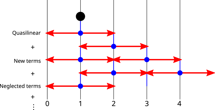
Figure 1: Diagram used to find the order in $\tau_{c}$ of the neglected terms.

In figure 1, the vertical lines denote functional derivatives of various orders. Starting from the RHS of equation 27 (black circle), one obtains various terms after repeated application of the recursion relation (equation 69 or 26; in the figure, each blue circle with arrows leading out corresponds to one application of the relation). A rightward step adds two time integrals and a velocity correlation, while a leftward step introduces neither velocity correlations nor time integrals. The order of a particular term in $\tau_{c}$ is thus simply the number of rightward steps taken to reach it, starting from the black circle. The terms we have neglected are $O(\tau_{c}^{2})$.

3.3 Simplification assuming separable, weakly inhomogeneous turbulence

3.3.1 Assumptions

Assuming $\kappa=0$ (which corresponds to $\Pen\gg 1$; $\Pen$, the Peclet number, is the ratio of the diffusive timescale to the advective timescale for the total passive scalar), we simplify the terms on the RHS of equation 28 in appendix D. The expressions obtained are somewhat long. We proceed by assuming the velocity correlations are separable, i.e.

$$\left<u_{i}(\boldsymbol{x},t+\tau)\partial^{n}_{i_{1}\dots i_{n}}u_{j}(\boldsymbol{x},t)\right>=C_{iji_{1}\dots i_{n}}(\boldsymbol{x},t)\mathfrak{D}(\tau)\,.$$ (29)

The temporal correlation function, $\mathfrak{D}$, has the properties

$$2\int_{0}^{\infty}\mathfrak{D}(t)\,\mathrm{d}t=1\,,\quad 2\int_{0}^{\infty}t\,\mathfrak{D}(t)\,\mathrm{d}t=\tau_{c}\,,$$ (30)

where $\tau_{c}$ is the correlation time. Note that we have assumed the correlation time is independent of the spatial scale. We further assume that $C(\boldsymbol{x},t)$ and $\left<\lambda_{i}(\boldsymbol{x},t)\right>$ vary on a timescale much larger than the timescale of $\mathfrak{D}(\tau)$. Discarding terms with more than two derivatives of the mean scalar field ($\Phi$) and taking the ‘weakly inhomogeneous’ case (where we keep only one large-scale derivative of the turbulent spectra; see appendix C), we obtain simple expressions, which we describe below.

3.3.2 The diffusion equation for the mean scalar

Name	$\mathfrak{D}(\tau)$	$g_{2}$
Exponential	$\displaystyle\frac{1}{2\tau_{c}}\,e^{-\left|\tau\right|/\tau_{c}}$	1/8
Top hat	$\displaystyle\frac{1}{4\tau_{c}}\,\operatorname{\text{$\Theta$}}{\!\left(2\tau_{c}-\tau\right)}\operatorname{\text{$\Theta$}}{\!\left(\tau+2\tau_{c}\right)}$	1/12

Table 1: Values of $g_{2}$ for some temporal correlation functions. The corresponding values of $g_{1}$ can be calculated using equation 71. The constants in the correlation functions have been chosen to satisfy equations 30.

Setting $\kappa=0$, the average of the evolution equation for the total passive scalar (equation 1)

$$\frac{\partial\Phi}{\partial t}=-\left<\boldsymbol{u}\cdot\nabla\theta\right>$$ (31)

Using equations 100, 101, and 102 (appendix D.4), we write the above as

$$\frac{\partial\Phi}{\partial t}=\frac{\partial}{\partial x_{i}}{\left[\left(\frac{E}{3}+\frac{\tau_{c}g_{1}H^{2}}{18}-\frac{\tau_{c}2g_{2}EN}{9}\right)\frac{\partial\Phi}{\partial x_{i}}\right]}\,.$$ (32)

where $g_{1}$ and $g_{2}$ depend on the temporal correlation function $\mathfrak{D}(\tau)$ (table 1 lists some examples), and

$$E(\boldsymbol{x},t)\equiv{} \int_{0}^{\infty}\left<u_{i}(\boldsymbol{x},t+\tau)u_{i}(\boldsymbol{x},t)\right>\mathrm{d}\tau$$ (33a)

$$H(\boldsymbol{x},t)\equiv{} 2\int_{0}^{\infty}\left<u_{i}(\boldsymbol{x},t+\tau)\omega_{i}(\boldsymbol{x},t)\right>\mathrm{d}\tau$$ (33b)

$$N(\boldsymbol{x},t)\equiv{} 2\int_{0}^{\infty}\left<\omega_{i}(\boldsymbol{x},t+\tau)\omega_{i}(\boldsymbol{x},t)\right>\mathrm{d}\tau\,.$$ (33c)

Note that the definition of $E$ is consistent with that in equation 9.

For a maximally helical velocity field with a top-hat temporal correlation function ($g_{2}=1/12$ and $H^{2}=2EN$), the $O(\tau_{c})$ correction to the turbulent diffusivity becomes zero. On the other hand, if the temporal correlation function is exponential, we obtain

$$\frac{\partial\Phi}{\partial t}=\frac{\partial}{\partial x_{i}}{\left[\left(\frac{E}{3}-\frac{\tau_{c}}{144}\left(4EN-H^{2}\right)\right)\frac{\partial\Phi}{\partial x_{i}}\right]}+O(\tau_{c}^{2})\,.$$ (34)

Note that the $O(\tau_{c})$ terms in this case cannot be zero, since the Cauchy-Schwarz inequality guarantees that $H^{2}\leq 2EN$. The corrections above match those obtained by Drummond (1982, eq. 5.1) and Knobloch (1977, eq. 38).

Examination of equation 32 shows that for weakly inhomogeneous turbulence, the effective diffusivity becomes negative when $\tau_{c}N(2g_{2}-g_{1}f^{2})>3$ (where we have defined $f^{2}\equiv H^{2}/2EN\in[0,1]$) and is positive otherwise. However, when the $O(\tau_{c})$ corrections are so strong, one would expect the neglected $O(\tau_{c}^{2})$ terms to also become non-negligible, making equation 32 invalid.

3.3.3 Validity of the expansion

We now make a crude estimate of how $\tau_{c}N$, which controls the validity of equation 34, depends on $\Rey$. Assuming the velocity field is homogeneous and isotropic, we estimate (recall that $N$ was defined in equation 33)

$$N\propto\int k^{2}\widetilde{C}_{ii}(k)\,\mathrm{d}\boldsymbol{k}$$ (35)

where $\widetilde{C}_{ii}$ is the Fourier transform of $C_{ii}$ (equation 29). Let us assume $\widetilde{C}_{ii}(k)$ is a power law in $k_{0}<k<k_{\nu}$ (which we refer to as the inertial range) and zero elsewhere. If we assume the velocity field obeys the Kolmogorov scaling relations (e.g. Davidson, 2004, section 1.6) in the inertial range, the fact that $C_{ii}(\boldsymbol{x})$ is dimensionally a diffusivity implies $\widetilde{C}_{ii}(k)\sim k^{-13/3}$. We then estimate

$$N\propto\int_{k_{0}}^{k_{\nu}}k^{-1/3}\mathrm{d}k\propto k_{\nu}^{2/3}-k_{0}^{2/3}\approx k_{\nu}^{2/3}$$ (36)

where the last step assumes $k_{\nu}\gg k_{0}$. Similarly, we can also estimate $E\sim k_{0}^{-4/3}$, which gives us $N/(Ek_{0}^{2})\propto\Rey^{1/2}$. Defining $\mbox{{St}}\equiv\tau_{c}Ek_{0}^{2}$, we then find

$$\tau_{c}N\propto\mbox{{St}}\,\Rey^{1/2}\,.$$ (37)

This means that for equation 34 to be valid, we require both the Strouhal number and the Reynolds number to not be large. We believe the latter limitation is due to our assumption that the velocity field at all scales can be characterized by a single scale-independent correlation time ($\tau_{c}$).

3.4 Aside: validity of the quasilinear approximation

Let us now try to understand the regimes in which the quasilinear approximation is valid. From the discussion above, it is clear that the quasilinear approximation becomes valid when the correlation time of the velocity field approaches zero.

There is also another limit in which the quasilinear approximation is valid. Even when the correlation time is nonzero, one may expect the quasilinear approximation to remain valid if the $O(\tau_{c})$ corrections from the quasilinear approximation (section 2.4) are much larger than the $O(\tau_{c})$ contributions from the second and third terms on the RHS of equation 28. We may estimate the ratios of these contributions as

$$\frac{\text{post-quasilinear}}{\text{quasilinear}}\sim\left.\left(\frac{\tau^{3}u^{4}}{l^{4}}\Phi\right)\middle/\left(\frac{\tau^{2}u^{2}}{l^{2}}\,\frac{\partial\Phi}{\partial t}\right)\right.$$ (38)

where $l$ denotes a length scale typical of the spatial derivative of an averaged quantity, $\tau$ denotes the correlation time of the fluctuating velocity field, and $u$ is the RMS value of the fluctuating velocity field. If we further use equation 12 for $\partial\Phi/\partial t$, we can write

$$\frac{\text{post-quasilinear}}{\text{quasilinear}}\sim\frac{\tau u^{2}}{\kappa+\tau u^{2}/3}\,.$$ (39)

Estimating $\tau\sim l/u$ (i.e. $St\sim 1$), we find

$$\frac{\text{post-quasilinear}}{\text{quasilinear}}\sim\frac{\Pen}{1+\Pen/3}\,.$$ (40)

where $\Pen\equiv ul/\kappa$. We thus see that even if the correlation time of the velocity field is not small, the quasilinear approximation can remain valid as long as $\Pen$ is small.

4 Magnetic field transport with nonzero correlation time

4.1 Application of the Furutsu-Novikov theorem

Let us consider the induction equation with constant $\eta$:

$$\frac{\partial\boldsymbol{B}}{\partial t}=\nabla\!\times\!\left(\boldsymbol{u}\times\boldsymbol{B}\right)+\eta\nabla^{2}\boldsymbol{B}\,.$$ (41)

For simplicity, we assume $\left<\boldsymbol{u}\right>=\boldsymbol{0}$. Averaging both sides, we find that the equation for the mean magnetic field is

$$\frac{\partial\overline{\boldsymbol{B}}}{\partial t}=\nabla\!\times\!\boldsymbol{\mathcal{E}}+\eta\nabla^{2}\overline{\boldsymbol{B}}$$ (42)

where

$$\boldsymbol{\mathcal{E}}\equiv\left<\boldsymbol{u}\times\boldsymbol{b}\right>\,,\quad\boldsymbol{b}\equiv\boldsymbol{B}-\overline{\boldsymbol{B}}{}\,.$$ (43)

To solve for the evolution of the mean magnetic field without solving for the fluctuating fields, we require an expression for $\boldsymbol{\mathcal{E}}$ that depends only on known statistical properties of the velocity field and on $\overline{\boldsymbol{B}}$.

Treating the first term on the RHS of equation 41 as a source, we can write the magnetic field at some arbitrary time as (analogous to equation 16 for the passive scalar)

$$B_{i}(\boldsymbol{x},t)=\int_{-\infty}^{t}\mathrm{d}\tau\int\mathrm{d}\boldsymbol{q}\,G(\boldsymbol{x},t|\boldsymbol{q},\tau)\,\epsilon_{ijk}\epsilon_{klm}\frac{\partial}{\partial q_{j}}\left(u_{l}(\boldsymbol{q},\tau)B_{m}(\boldsymbol{q},\tau)\right)\,.$$ (44)

We assume $\boldsymbol{u}$ is a Gaussian random field. Recalling that $\left<\boldsymbol{u}\right>=\boldsymbol{0}$, the EMF can be written as $\boldsymbol{\mathcal{E}}=\left<\boldsymbol{u}\times\boldsymbol{B}\right>$. The Furutsu-Novikov theorem (equation 15) takes the form

$$\begin{split}\left<u_{i}(\boldsymbol{x},t)B_{j}(\boldsymbol{x},t)\right>=\int\mathrm{d}\boldsymbol{x}^{\prime}\mathrm{d}t^{\prime}\left<u_{i}(\boldsymbol{x},t)u_{k}(\boldsymbol{x}^{\prime},t^{\prime})\right>\left<\frac{\delta B_{j}(\boldsymbol{x},t)}{\delta u_{k}(\boldsymbol{x}^{\prime},t^{\prime})}\right>\,.\end{split}$$ (45)

For the sake of brevity, we will use notation similar to that described on page 25. Explicitly,

$$\begin{split}\left.\boxed{\boxed{\frac{\beta_{m}}{1_{j_{1}}\dots n_{j_{n}}}}}\right.\equiv{}&\left<\frac{\delta^{n}\lambda_{m}\leavevmode\hbox to10.52pt{\vbox to10.52pt{\text{[drawing]}}}}{\delta u_{j_{1}}\leavevmode\hbox to8.9pt{\vbox to8.9pt{\text{[drawing]}}}\dots u_{j_{n}}\leavevmode\hbox to8.38pt{\vbox to8.38pt{\text{[drawing]}}}}\right>\end{split} \beta 1 n$$ (46)

$$\begin{split}\Game_{m}(1|2)\equiv{}&\eth^{(2)}_{m}G^{c}\!(\leavevmode\hbox to8.9pt{\vbox to8.9pt{\text{[drawing]}}}|\leavevmode\hbox to8.9pt{\vbox to8.9pt{\text{[drawing]}}})\end{split} 1 2$$ (47)

$$\begin{split}\Upsilon_{ijlm}\equiv{}&\epsilon_{ijk}\epsilon_{klm}\,.\end{split}$$ (48)

The average of the $n$-th functional derivative of $B$ (derived in appendix E as equation 106) can then be written as

$$\begin{split}\left.\boxed{\boxed{\frac{\maltese_{i}}{1_{i_{1}}\dots n_{i_{n}}}}}\right.={}&-\int\mathrm{d}A\mathrm{d}B\,\Game_{j}(\maltese|\leavevmode\hbox to10.32pt{\vbox to10.32pt{\text{[drawing]}}})\Upsilon_{ijlm}\left.\boxed{A_{l}B_{a}}\right.\left.\boxed{\boxed{\frac{A_{m}}{1_{i_{1}}\dots n_{i_{n}}B_{a}}}}\right.\\ &-\sum_{\alpha=1}^{n}\Game_{j}(\maltese|\leavevmode\hbox to8.57pt{\vbox to8.57pt{\text{[drawing]}}})\Upsilon_{iji_{\alpha}m}\left.\boxed{\boxed{\frac{\alpha_{m}}{1_{i_{1}}\dots(\alpha-1)_{i_{\alpha-1}}(\alpha+1)_{i_{\alpha+1}}\dots n_{i_{n}}}}}\right.\,.\end{split} A \alpha$$ (49)

Henceforth, we adopt the convention that $\maltese$ is the only variable that is not integrated over. Equation 45 can be written as

$$\begin{split}\phantom{===}&\hskip-23.3334pt\left<u_{i}(\boldsymbol{x},t)B_{j}(\boldsymbol{x},t)\right>=\left.\boxed{\maltese_{i}1_{k}}\right.\left.\boxed{\boxed{\frac{\maltese_{j}}{1_{k}}}}\right.\end{split}$$ (50)

$$\begin{split}={}&-\Upsilon_{ji_{2}i_{1}i_{3}}\left.\boxed{{\maltese}_{i}{1}_{i_{1}}}\right.\Game_{i_{2}}(\maltese|1)\overline{B}_{i_{3}}\leavevmode\hbox to8.9pt{\vbox to8.9pt{\text{[drawing]}}}\\ &-\Upsilon_{i_{5}i_{6}i_{1}i_{7}}\Upsilon_{jj_{3}i_{2}j_{2}}\Upsilon_{j_{2}i_{4}i_{3}i_{5}}\left.\boxed{{\maltese}_{i}{1}_{i_{1}}}\right.\Game_{j_{3}}(\maltese|2)\left.\boxed{{2}_{i_{2}}{3}_{i_{3}}}\right.\Game_{i_{4}}(2|3)\Game_{i_{6}}(3|1)\overline{B}_{i_{7}}\leavevmode\hbox to8.9pt{\vbox to8.9pt{\text{[drawing]}}}\\ &-\Upsilon_{i_{5}i_{6}i_{3}i_{7}}\Upsilon_{jj_{3}i_{2}j_{2}}\Upsilon_{j_{2}i_{4}i_{1}i_{5}}\left.\boxed{{\maltese}_{i}{1}_{i_{1}}}\right.\Game_{j_{3}}(\maltese|2)\left.\boxed{{2}_{i_{2}}{3}_{i_{3}}}\right.\Game_{i_{4}}(2|1)\Game_{i_{6}}(1|3)\overline{B}_{i_{7}}\leavevmode\hbox to8.9pt{\vbox to8.9pt{\text{[drawing]}}}\end{split} 1 1 3$$ (51)

where we have applied the relation 49 thrice and discarded terms with more than two velocity correlations. As argued in the case of the passive scalar (section 3), the first term is $O(\tau_{c}^{0})$ (but also contains $O(\tau_{c})$ contributions), while the next two terms are $O(\tau_{c})$, where $\tau_{c}$ is the correlation time of the velocity field.

4.2 The white-noise limit

The $O(\tau_{c}^{0})$ term of equation 51 is

$$\left<u_{i}B_{j}\right>={} -\Upsilon_{ji_{2}i_{1}i_{3}}\left.\boxed{{\maltese}_{i}{1}_{i_{1}}}\right.\Game_{i_{2}}(\maltese|1)\overline{B}_{i_{3}}\leavevmode\hbox to8.9pt{\vbox to8.9pt{\text{[drawing]}}} 1$$ (52)

$$\begin{split}={}&-\Upsilon_{ji_{2}i_{1}i_{3}}\int\mathrm{d}\boldsymbol{x}^{\prime}\mathrm{d}t^{\prime}\left<u_{i}(\boldsymbol{x},t)u_{i_{1}}(\boldsymbol{x}^{\prime},t^{\prime})\right>\frac{\partial G^{c}(\boldsymbol{x},t|\boldsymbol{x}^{\prime},t^{\prime})}{\partial x^{\prime}_{i_{2}}}\overline{B}_{i_{3}}(\boldsymbol{x}^{\prime},t^{\prime})\,.\end{split}$$ (53)

Assuming $\eta=0$ and discarding the $O(\tau_{c})$ parts of this term, we find that

$$\begin{split}\left<u_{i}B_{j}\right>={}&\Upsilon_{ji_{2}i_{1}i_{3}}\int_{-\infty}^{t}\mathrm{d}t^{\prime}\,\left<u_{i}(\boldsymbol{x},t)\frac{\partial}{\partial x_{i_{2}}}u_{i_{1}}(\boldsymbol{x},t^{\prime})\right>\overline{B}_{i_{3}}(\boldsymbol{x},t)\\ &+\Upsilon_{ji_{2}i_{1}i_{3}}\int_{-\infty}^{t}\mathrm{d}t^{\prime}\,\left<u_{i}(\boldsymbol{x},t)u_{i_{1}}(\boldsymbol{x},t^{\prime})\right>\frac{\partial\overline{B}_{i_{3}}(\boldsymbol{x},t)}{\partial x_{i_{2}}}\,.\end{split}$$ (54)

Assuming the velocity correlations are separable (equation 29) and the turbulence is homogeneous, we can use the expressions from appendix C.3 and write

$$\begin{split}\left<V_{i}B_{j}\right>={}&\frac{1}{12}\epsilon_{ii_{2}j}H\overline{B}_{i_{2}}-\frac{E}{3}\,\frac{\partial\overline{B}_{j}}{\partial x_{i}}\end{split}$$ (55)

where we have used the fact that the divergence of the magnetic field is zero. The EMF can then be written as

$$\mathcal{E}_{k}=\epsilon_{kij}\left<V_{i}B_{j}\right>=-\frac{H}{6}\,\overline{B}_{k}-\frac{E}{3}\,\epsilon_{kij}\partial_{i}\overline{B}_{j}$$ (56)

which is exactly the same as the usual quasilinear expression (e.g. Moffatt, 1978, chapter 7). This is usually written in the form

$$\mathcal{E}_{k}=\alpha\,\overline{B}_{k}-\eta\,\epsilon_{kij}\partial_{i}\overline{B}_{j}\,.$$ (57)

The coefficient $\alpha$ describes how a helical velocity field can drive the growth of a mean magnetic field, while the coefficient $\eta$ (called the turbulent diffusivity) describes dissipation of a mean magnetic field through the action of turbulence.

4.3 Corrections due to nonzero correlation time

4.3.1 Expression for the EMF

In appendix F, we simplify all the three terms on the RHS of equation 51, keeping $O(\tau_{c})$ contributions, assuming the turbulence is homogeneous and isotropic, and setting $\eta=0$. Setting $\eta=0$ in these terms corresponds to assuming $\mbox{{Rm}}\gg 1$ (Rm, the magnetic Reynolds number, is the ratio of the diffusive timescale to the advective timescale for the total magnetic field). The overall contribution to the EMF ($\mathcal{E}_{k}=\epsilon_{kij}\left<V_{i}B_{j}\right>$, the contributions to which are given by equations 112, 115 and 118) is

$$\begin{split}\mathcal{E}_{k}={}&\left(\alpha_{0}+\tau_{c}\alpha_{1}\right)\overline{B}{}_{k}-\left(\eta_{0}-\tau_{c}\eta_{1}\right)\epsilon{}_{kr_{0}r_{1}}\partial_{r_{0}}\overline{B}{}_{r_{1}}\,.\end{split}$$ (58)

Above, $\alpha_{0}$ and $\eta_{0}$ are the coefficients when the correlation time is zero (equation 57);

$$\begin{split}\alpha_{1}\equiv{}&\frac{g_{2}}{9}\left(2EL+HN\right)\,,\end{split}$$ (59)

$$\begin{split}\eta_{1}\equiv{}&\frac{2ENg_{2}}{9}+\frac{H^{2}g_{2}}{18}+\frac{H^{2}}{24}\,;\end{split}$$ (60)

we have eliminated $g_{1}$ by using the fact that $g_{1}+g_{2}=1/4$ (equation 71); $E$, $H$, and $N$ are defined in equations 33; and

$$L(\boldsymbol{x},t)\equiv 2\int_{0}^{\infty}\left<\boldsymbol{\omega}(\boldsymbol{x},t+\tau)\cdot\left[\nabla\!\times\!\boldsymbol{\omega}(\boldsymbol{x},t)\right]\right>\mathrm{d}\tau\,.$$ (61)

Note that the turbulent diffusivity is always reduced by the $O(\tau_{c})$ terms. The validity of this equation is also determined by the criterion given in section 3.3.3.

Denoting the turbulent diffusivity for the mean magnetic field as $\eta_{B}$, and that for the mean passive scalar (equation 32) as $\eta_{\theta}$, we find that

$$\eta_{B}-\eta_{\theta}=-\tau_{c}H^{2}\left(\frac{g_{1}+g_{2}}{18}+\frac{1}{24}\right)=-\frac{\tau_{c}H^{2}}{18}$$ (62)

where we have used $g_{1}+g_{2}=1/4$ (equation 71). Note that this is independent of the form of the temporal correlation function of the velocity field.

4.3.2 Comparison with the cumulant expansion

Knobloch (1977) and Nicklaus & Stix (1988) have also studied such corrections using the cumulant expansion. In particular, Nicklaus & Stix (1988, eqs. 24,26) have further simplified their results by treating the velocity field as a Gaussian random field. Our results are expected to agree with theirs for $t\gg\tau_{c}$. Our corrections to the $\alpha$ effect indeed match theirs. However, their stated correction to the turbulent diffusivity of the magnetic field differs from our result above, and is instead identical to what we had obtained for passive scalar diffusion (equation 32).

The expression given by Knobloch (1977, eq. 42) for the difference between the magnetic and scalar diffusivities can be simplified by assuming the velocity correlation is separable (equation 29). However, the resulting expression contains an integral of the form $\int_{0}^{t}\mathrm{d}t_{1}\int_{0}^{t_{1}}\mathrm{d}t_{2}\int_{0}^{t_{2}}\mathrm{d}t_{3}\,\mathfrak{D}(t-t_{1})\,\mathfrak{D}(t_{2}-t_{3})$; this integral diverges as $O(t;t\to\infty)$. It is unclear if this divergence is due to missed terms in their calculations, or a limitation of the cumulant expansion. We note that the results reported by Nicklaus & Stix (1988, eqs. 24,26) do not have this problem as the coefficient of this integral in their expressions turns out to be zero if the velocity field is Gaussian.

4.3.3 Relation to the $\alpha^{2}$ effect

The negative contribution to the turbulent diffusivity in equation 58 is reminiscent of that obtained by Kraichnan (1976, eq. 4.8) using a multi-scale averaging procedure. However, in the calculations reported by Kraichnan (1976), the helicity of the velocity field does not have any effect on the mean passive scalar; he attributes this to differences between the conservation properties of the passive scalar and the magnetic field (Kraichnan, 1976, p. 659). This is contrary to our finding that helicity can even suppress the diffusion of the mean passive scalar (equation 32). The fact that our $O(\tau_{c})$ correction to the turbulent diffusivity of the mean passive scalar becomes zero when the temporal correlation function is given by a top hat suggests that the results of Kraichnan (1976) are attributable to his use of a ‘renovating flow’ model (which corresponds to such a temporal correlation function).

4.3.4 Comparison with renormalization group theory

In simulations of forced turbulence, Brandenburg et al. (2017, fig. 4) found that the turbulent diffusivity is smaller when the turbulence is helically forced than when it is nonhelically forced. Further, they found that for small Rm, the helicity-dependent correction to the turbulent diffusivity of the magnetic field scales as $\mbox{{Rm}}^{2}$. This was later confirmed by Mizerski (2023) using renormalization group theory. Since we have focused on the limit of high Rm, we do not recover this scaling.

Mizerski (2023, eq. 18) also derived a correction to the turbulent diffusivity in the limit of small fractional helicity and large Rm. This correction seems consistent with our result (in the sense that the difference between the diffusivity in a helical velocity field and that in a nonhelical velocity field depends on the square of the helicity). While we assume a single scale-independent correlation time, the method used by Mizerski (2023) allows the scale-dependent correlation time to be determined by the equations of motion (and thus it does not appear as a free parameter). Note that Mizerski (2023) do not seem to have calculated the corrections to the $\alpha$ effect (see our equation 58); nevertheless, we expect such corrections to be obtainable using their method.

5 Conclusions

Conventional treatments of mean-field theory use the quasilinear approximation to derive expressions for transport coefficients which are exact when the correlation time of the velocity field is zero. Assuming the velocity field is a Gaussian random field with a nonzero correlation time, we have applied the Furutsu-Novikov theorem to find the lowest-order corrections to the transport coefficients for two kinds of passive tensors.

For the diffusion of the mean passive scalar in the limit of high Peclet number, we have verified that our result matches earlier results obtained through different methods (Drummond, 1982; Knobloch, 1977). Using the multi-scale averaging approach, Kraichnan (1976) has reported that the helicity of the velocity field does not affect the turbulent diffusion of the passive scalar. We have found that this is only the case for a specific form of the temporal correlation function of the velocity field, corresponding to the renovating flow model used in that work.

We have also considered the mean magnetic field (treated, in the kinematic limit, as a passive pseudovector) at high magnetic Reynolds number, and found that both the $\alpha$ effect and magnetic diffusion are affected by the correlation time of the velocity field. An earlier result for the diffusivity of the mean magnetic field (Nicklaus & Stix, 1988, eqs. 24,26) turns out to be identical to that for the mean passive scalar; we obtain extra (negative) contributions to the diffusivity of the mean magnetic field.

The validity of the expressions we have derived is limited by our assumption that the correlation time of the velocity field is scale-independent. While the general formalism we have used can be adapted to account for a scale-dependent correlation time, this is left to future work.

[Acknowledgements] We thank Alexandra Elbakyan for facilitating access to scientific literature. We acknowledge discussions with Matthias Rheinhardt, Igor Rogachevskii, Axel Brandenburg, and Petri Käpylä.

[Funding] This research received no specific grant from any funding agency, commercial or not-for-profit sectors.

[Software] Sympy (Meurer et al., 2017).

[Declaration of interests] The authors report no conflict of interest.

[Author ORCID] GK, https://orcid.org/0000-0003-2620-790X; NS, https://orcid.org/0000-0001-6097-688X

[Author contributions] GK and NS conceptualized the research, interpreted the results, and wrote the paper. GK performed the calculations.

Appendix A $n$-th functional derivative of $\nabla\theta$

We first recall the definition of the $n$-th functional derivative of a functional $F[f]$ wrt. a function $f(t)$:

$$\left.\frac{\mathrm{d}^{n}F[f+\epsilon\chi]}{\mathrm{d}\epsilon^{n}}\right|_{\epsilon=0}=\int\frac{\delta^{n}F}{\delta f(t_{1})\dots\delta f(t_{n})}\chi(t_{1})\dots\chi(t_{n})\,\mathrm{d}t_{1}\dots\mathrm{d}t_{n}$$ (63)

where $\epsilon$ is a real number, and $\chi(t)$ is an arbitrary test function.

Using the same notation as in section 3, we write (similar to equation 17)

$$\lambda_{i}(\boldsymbol{x},t)=-\frac{\partial}{\partial x_{i}}\int_{-\infty}^{t}\mathrm{d}\tau\int\mathrm{d}\boldsymbol{q}\,G(\boldsymbol{x},t|\boldsymbol{q},\tau)\,u_{m}(\boldsymbol{q},\tau)\lambda_{m}(\boldsymbol{q},\tau)\,.$$ (64)

Denoting $\bar{\lambda}\equiv\lambda[u_{m}+\epsilon\chi_{m}]$, we write

$$\bar{\lambda}_{i}(\boldsymbol{x},t)=-\frac{\partial}{\partial x_{i}}\int_{-\infty}^{t}\mathrm{d}\tau\int\mathrm{d}\boldsymbol{q}\,G(\boldsymbol{x},t|\boldsymbol{q},\tau)\left(u_{m}(\boldsymbol{q},\tau)+\epsilon\chi_{m}(\boldsymbol{q},\tau)\right)\bar{\lambda}_{m}(\boldsymbol{q},\tau)\,.$$ (65)

Taking $n$ derivatives on both sides and setting $\epsilon=0$, we write

$$\begin{split}\left.\frac{\mathrm{d}^{n}\bar{\lambda}_{i}(\boldsymbol{x},t)}{\mathrm{d}\epsilon^{n}}\right|_{\epsilon=0}={}&-\frac{\partial}{\partial x_{i}}\int_{-\infty}^{t}\mathrm{d}\tau\int\mathrm{d}\boldsymbol{q}\,G(\boldsymbol{x},t|\boldsymbol{q},\tau)\,u_{m}(\boldsymbol{q},\tau)\left.\frac{\mathrm{d}^{n}\bar{\lambda}_{m}(\boldsymbol{q},\tau)}{\mathrm{d}\epsilon^{n}}\right|_{\epsilon=0}\\ &-n\frac{\partial}{\partial x_{i}}\int_{-\infty}^{t}\mathrm{d}\tau\int\mathrm{d}\boldsymbol{q}\,G(\boldsymbol{x},t|\boldsymbol{q},\tau)\,\chi_{m}(\boldsymbol{q},\tau)\left.\frac{\mathrm{d}^{n-1}\bar{\lambda}_{m}(\boldsymbol{q},\tau)}{\mathrm{d}\epsilon^{n-1}}\right|_{\epsilon=0}\end{split}$$ (66)

which gives us the following relation between the functional derivatives (we use the notation $u_{j_{i}}\equiv u_{j_{i}}(\boldsymbol{x}^{(i)},t^{(i)})$):

$$\begin{split}\frac{\delta^{n}\lambda_{i}(\boldsymbol{x},t)}{\delta u_{j_{1}}\dots\delta u_{j_{n}}}={}&-\frac{\partial}{\partial x_{i}}\int\mathrm{d}\boldsymbol{q}\int_{\operatorname{max}(t^{(1)},\dots,t^{(n)})}^{t}\hskip-45.00006pt\mathrm{d}\tau\,G(\boldsymbol{x},t|\boldsymbol{q},\tau)\,u_{m}(\boldsymbol{q},\tau)\,\frac{\delta^{n}\lambda_{m}(\boldsymbol{q},\tau)}{\delta u_{j_{1}}\dots\delta u_{j_{n}}}\\ &-\sum_{\alpha=1}^{n}\frac{\partial}{\partial x_{i}}G(\boldsymbol{x},t|\boldsymbol{x}^{(\alpha)},t^{(\alpha)})\operatorname{\text{$\Theta$}}(t-t^{(\alpha)})\,\frac{\delta^{n-1}\lambda_{j_{\alpha}}(\boldsymbol{x}^{(\alpha)},t^{(\alpha)})}{\delta u_{j_{1}}\dots\delta u_{j_{\alpha-1}}\delta u_{j_{\alpha+1}}\dots\delta u_{j_{n}}}\,.\end{split}$$ (67)

We average both sides of the above and use the Furutsu-Novikov theorem (equation 15) to write

$$\begin{split}&\left<\frac{\delta^{n}\lambda_{i}(\boldsymbol{x},t)}{\delta u_{j_{1}}\dots\delta u_{j_{n}}}\right>\\ &=-\frac{\partial}{\partial x_{i}}\int\mathrm{d}\boldsymbol{q}\mathrm{d}\boldsymbol{x}^{\prime}\mathrm{d}t^{\prime}\int_{\operatorname{max}(t^{(1)},\dots,t^{(n)})}^{t}\hskip-45.00006pt\mathrm{d}\tau\,G(\boldsymbol{x},t|\boldsymbol{q},\tau)\left<u_{m}(\boldsymbol{q},\tau)u_{a}(\boldsymbol{x}^{\prime},t^{\prime})\right>\left<\frac{\delta^{n+1}\lambda_{m}(\boldsymbol{q},\tau)}{\delta u_{a}(\boldsymbol{x}^{\prime},t^{\prime})\delta u_{j_{1}}\dots\delta u_{j_{n}}}\right>\\ &\phantom{={}}-\sum_{\alpha=1}^{n}\frac{\partial}{\partial x_{i}}G(\boldsymbol{x},t|\boldsymbol{x}^{(\alpha)},t^{(\alpha)})\operatorname{\text{$\Theta$}}(t-t^{(\alpha)})\left<\frac{\delta^{n-1}\lambda_{j_{\alpha}}(\boldsymbol{x}^{(\alpha)},t^{(\alpha)})}{\delta u_{j_{1}}\dots\delta u_{j_{\alpha-1}}\delta u_{j_{\alpha+1}}\dots\delta u_{j_{n}}}\right>\,.\end{split}$$ (68)

By taking causality into account ($\delta\lambda(t)/\delta u(t^{\prime})=0$ if $t^{\prime}>t$) we can write the above more compactly as

$$\begin{split}&\left<\frac{\delta^{n}\lambda_{i}(\boldsymbol{x},t)}{\delta u_{j_{1}}\dots\delta u_{j_{n}}}\right>\\ &=-\frac{\partial}{\partial x_{i}}\int\mathrm{d}\boldsymbol{q}\mathrm{d}\boldsymbol{x}^{\prime}\mathrm{d}t^{\prime}\mathrm{d}\tau\,G^{c}\!(\boldsymbol{x},t|\boldsymbol{q},\tau)\left<u_{m}(\boldsymbol{q},\tau)u_{a}(\boldsymbol{x}^{\prime},t^{\prime})\right>\left<\frac{\delta^{n+1}\lambda_{m}(\boldsymbol{q},\tau)}{\delta u_{a}(\boldsymbol{x}^{\prime},t^{\prime})\delta u_{j_{1}}\dots\delta u_{j_{n}}}\right>\\ &\phantom{={}}-\sum_{\alpha=1}^{n}\frac{\partial}{\partial x_{i}}G^{c}\!(\boldsymbol{x},t|\boldsymbol{x}^{(\alpha)},t^{(\alpha)})\left<\frac{\delta^{n-1}\lambda_{j_{\alpha}}(\boldsymbol{x}^{(\alpha)},t^{(\alpha)})}{\delta u_{j_{1}}\dots\delta u_{j_{\alpha-1}}\delta u_{j_{\alpha+1}}\dots\delta u_{j_{n}}}\right>\,.\end{split}$$ (69)

Note the superscript ‘$c$’ on the Green function, which denotes that it has been made causal ($G^{c}\!(x,t|x^{\prime},t^{\prime})=0$ if $t^{\prime}>t$; $G(x,t|x^{\prime},t^{\prime})$ otherwise).

Appendix B Coefficients that depend on the temporal correlation function

Our results depend on the form of the temporal correlation function of the velocity field only through the following coefficients:

$$\begin{split}g_{1}&{}\equiv\frac{1}{\tau_{c}}\int_{-\infty}^{t}\mathrm{d}t^{\prime}\int_{-\infty}^{t^{\prime}}\mathrm{d}t_{1}\int_{-\infty}^{t_{1}}\mathrm{d}t_{2}\,\mathfrak{D}^{(t-t_{1})}\mathfrak{D}^{(t^{\prime}-t_{2})}\end{split}$$ (70a)

$$\begin{split}g_{2}&{}\equiv\frac{1}{\tau_{c}}\int_{-\infty}^{t}\mathrm{d}t^{\prime}\int_{-\infty}^{t^{\prime}}\mathrm{d}t_{2}\int_{-\infty}^{t_{2}}\mathrm{d}t_{1}\,\mathfrak{D}^{(t-t_{1})}\mathfrak{D}^{(t^{\prime}-t_{2})}\,.\end{split}$$ (70b)

The values of these coefficients depend on the form of the temporal correlation function (table 1). Regardless of the form of the temporal correlation function, they satisfy the identity (Gopalakrishnan & Singh, 2024, appendix C)

$$g_{1}+g_{2}=\frac{1}{4}\,.$$ (71)

Appendix C Velocity correlations for locally isotropic, weakly inhomogeneous turbulence

C.1 The equal-time correlation in Fourier-space

We define the Fourier transform as

$$\tilde{f}(\boldsymbol{k})=\int\frac{\mathrm{d}^{3}x}{(2\pi)^{3}}\,e^{-i\boldsymbol{k}\cdot\boldsymbol{x}}f(\boldsymbol{x})$$ (72)

and the two-point correlation of the Fourier transformed velocity field as $V_{ij}(\boldsymbol{k},\boldsymbol{K},t)\equiv\left<\tilde{u}_{i}(\tfrac{1}{2}\boldsymbol{K}+\boldsymbol{k},t)\tilde{u}_{j}(\tfrac{1}{2}\boldsymbol{K}-\boldsymbol{k},t)\right>$. If $\boldsymbol{k}_{1}$ and $\boldsymbol{k}_{2}$ denote the Fourier conjugates of the two positions between which the correlation is taken, $\boldsymbol{K}\equiv\boldsymbol{k}_{1}+\boldsymbol{k}_{2}$, and $\boldsymbol{k}\equiv(\boldsymbol{k}_{1}-\boldsymbol{k}_{2})/2$. We interpret $\boldsymbol{K}$ as the ‘large scale’ wavevector, and $\boldsymbol{k}$ as the ‘small scale’ wavevector. According to the notion of weak inhomogeneity introduced by Roberts & Soward (1975), one Taylor-expands this double correlation function function as a series in $\boldsymbol{K}$; assumes the lowest-order ($\boldsymbol{K}$-independent) terms are identical to those for homogeneous and isotropic turbulence (Moffatt, 1978, eq. 7.56; Lesieur, 2008, eq. 5.84); assumes that the higher-order terms only depend on the energy and helicity spectra (along with $\boldsymbol{k}$ and $\boldsymbol{K}$); and discards $O(K^{2})$ terms. Requiring the velocity field to be incompressible then leads to

$$\begin{split}V_{ij}(\boldsymbol{k},\boldsymbol{K},t)={}&\operatorname{P}_{ij}(\boldsymbol{k})E(k,\boldsymbol{K},t)-\frac{i}{k^{2}}\epsilon_{ijc}k_{c}F(k,\boldsymbol{K},t)\\ &+\frac{1}{2k^{2}}\left(k_{j}\delta_{ik}-k_{i}\delta_{jk}\right)K_{k}E(k,\boldsymbol{K},t)\\ &+\frac{i}{2k^{4}}\left(k_{i}\epsilon_{jck}+k_{j}\epsilon_{ick}\right)k_{c}K_{k}F(k,\boldsymbol{K},t)+O(K^{2})\,.\end{split}$$ (73)

C.2 Equal-time single-point correlations in real space

C.2.1 An example

As an example, we demonstrate how one can use equation 73 to derive an expression for $\left<u_{i}u_{j}\right>$ (an equal-time single-point correlation). We start from

$$\left<u_{i}(\boldsymbol{x})u_{j}(\boldsymbol{x})\right>=\int\mathrm{d}^{3}p\mathrm{d}^{3}q\,e^{i\left(\boldsymbol{p}+\boldsymbol{q}\right)\cdot\boldsymbol{x}}\left<\tilde{u}_{i}(\boldsymbol{q})\tilde{u}_{j}(\boldsymbol{p})\right>\,.$$ (74)

Defining $\boldsymbol{K}\equiv\boldsymbol{p}+\boldsymbol{q}$ and $\boldsymbol{k}\equiv\frac{1}{2}\left(\boldsymbol{p}-\boldsymbol{q}\right)$,

$$\left<u_{i}(\boldsymbol{x})u_{j}(\boldsymbol{x})\right>=\int\mathrm{d}^{3}K\mathrm{d}^{3}k\,e^{i\boldsymbol{K}\cdot\boldsymbol{x}}\left<\tilde{u}_{i}(\tfrac{1}{2}\boldsymbol{K}-\boldsymbol{k})\tilde{u}_{j}(\tfrac{1}{2}\boldsymbol{K}+\boldsymbol{k})\right>\,.$$ (75)

Using equation 73,

$$\begin{split}\left<u_{i}(\boldsymbol{x})u_{j}(\boldsymbol{x})\right>={}&\int\mathrm{d}^{3}Kk^{2}\mathrm{d}k\mathrm{d}\Omega_{k}\,e^{i\boldsymbol{K}\cdot\boldsymbol{x}}\bigg{(}\operatorname{P}_{ji}(\boldsymbol{k})E(k,\boldsymbol{K},t)-\frac{i}{k^{2}}\epsilon_{jic}k_{c}F(k,\boldsymbol{K},t)\\ &-\frac{1}{2k^{2}}k_{j}K_{i}E(k,\boldsymbol{K},t)+\frac{1}{2k^{2}}k_{i}K_{j}E(k,\boldsymbol{K},t)\\ &+\frac{i}{2k^{4}}k_{j}\epsilon_{icd}k_{c}K_{d}F(k,\boldsymbol{K},t)+\frac{i}{2k^{4}}k_{i}\epsilon_{jcd}k_{c}K_{d}F(k,\boldsymbol{K},t)\bigg{)}\,.\end{split}$$ (76)

Angular integrals over products of $\boldsymbol{k}$ can be evaluated by noting that the result has to be an isotropic tensor (and so needs to be constructed using $\delta_{ij}$ and $\epsilon_{ijk}$, Kearsley & Fong, 1975, e.g.) and must be consistent with the symmetries of the integrand:

$$\int\mathrm{d}\Omega\,k_{i}={} 0$$ (77)

$$\int\mathrm{d}\Omega\,k_{i}k_{j}={} \frac{4\pi k^{2}}{3}\delta_{ij}$$ (78)

$$\int\mathrm{d}\Omega\,k_{i}k_{j}k_{m}={} 0$$ (79)

$$\int\mathrm{d}\Omega\,k_{i}k_{j}k_{m}k_{n}={} \frac{4\pi k^{4}}{15}\left(\delta_{ij}\delta_{mn}+\delta_{im}\delta_{jn}+\delta_{in}\delta_{jm}\right)\,.$$ (80)

Using these, equation 76 can be written as

$$\begin{split}\left<u_{i}(\boldsymbol{x})u_{j}(\boldsymbol{x})\right>={}&\frac{1}{3}\delta_{ji}\left<u^{2}(\boldsymbol{x},t)\right>\,.\end{split}$$ (81)

The steps to derive the other expressions that follow are similar to those above, so we shall omit the intermediate steps and just state the results.

C.2.2 Results

$$\begin{split}\left<u_{i}u_{j}\right>={}&\frac{1}{3}\delta_{ji}\left<u^{2}\right>+O(\partial^{2})\end{split}$$ (82)

$$\begin{split}\left<u_{i}\frac{\partial u_{j}}{\partial x_{k}}\right>={}&\left[\frac{1}{6}\delta_{ij}\partial_{k}+\frac{1}{12}\left(\delta_{ik}\partial_{j}-\delta_{jk}\partial_{i}\right)\right]\left<u^{2}\right>-\frac{1}{6}\epsilon_{ijk}h+O(\partial^{2})\end{split}$$ (83)

$$\begin{split}\left<u_{i}\partial_{a}\partial_{b}u_{j}\right>={}&\frac{1}{12}\epsilon_{jia}\partial_{b}h+\frac{1}{12}\epsilon_{jib}\partial_{a}h+\left(\frac{1}{30}\left[\delta_{ai}\delta_{bj}+\delta_{aj}\delta_{bi}\right]-\frac{2}{15}\delta_{ab}\delta_{ij}\right)\left<\omega^{2}\right>\\ &-\frac{1}{60}\left(2\delta_{ab}\epsilon_{ijk}+\delta_{jb}\epsilon_{iak}+\delta_{aj}\epsilon_{ibk}+\delta_{ib}\epsilon_{jak}+\delta_{ai}\epsilon_{jbk}\right)\partial_{k}h+O(\partial^{2})\end{split}$$ (84)

$$\begin{split}\left<u_{i}\partial_{a}\nabla^{2}u_{j}\right>={}&\left(-\frac{1}{20}\delta_{ai}\partial_{j}+\frac{7}{60}\delta_{aj}\partial_{i}-\frac{3}{10}\delta_{ij}\partial_{a}\right)\left<\omega^{2}\right>-\frac{1}{6}\epsilon_{jia}\mathcal{L}+O(\partial^{2})\end{split}$$ (85)

where $\boldsymbol{\omega}\equiv\nabla\!\times\!\boldsymbol{u}$; $h\equiv\left<\boldsymbol{u}\cdot\boldsymbol{\omega}\right>$; and $\mathcal{L}\equiv\left<\boldsymbol{\omega}\cdot(\nabla\!\times\!\boldsymbol{\omega})\right>$. We have also used the relations $\left<\omega^{2}\right>(\boldsymbol{R},t)=\int 8\pi k^{4}E(k,\boldsymbol{R},t)\,\mathrm{d}k$ (Moffatt, 1978, eq. 7.51); and $\mathcal{L}(\boldsymbol{R},t)=\int\mathrm{d}k\,8\pi k^{4}F(k,\boldsymbol{R},t)$. Aside, we note that the expression given by Gopalakrishnan & Subramanian (2023, eq. A16) for $\left<u_{i}\partial_{a}\nabla^{2}u_{j}\right>$ is wrong.

C.3 Generalization to unequal-time correlations

Assuming the velocity correlations are separable (equation 29), the results in appendix C.2 can be easily generalized as

$$\begin{split}C_{ij}={}&\frac{2}{3}\delta_{ij}E\end{split}$$ (86)

$$\begin{split}C_{ijk}={}&\frac{1}{6}\epsilon_{ikj}H+\left[\frac{1}{3}\delta_{ij}\partial_{k}+\frac{1}{6}\left(\delta_{ik}\partial_{j}-\delta_{jk}\partial_{i}\right)\right]E\end{split}$$ (87)

$$\begin{split}C_{ijkk}={}&-\frac{1}{3}\delta_{ij}N-\frac{1}{6}\epsilon_{ija}\partial_{a}H\end{split}$$ (88)

$$\begin{split}C_{ijab}={}&\left(\frac{1}{30}\left[\delta_{ai}\delta_{bj}+\delta_{aj}\delta_{bi}\right]-\frac{2}{15}\delta_{ab}\delta_{ij}\right)N+\frac{1}{12}\epsilon_{jia}\partial_{b}H+\frac{1}{12}\epsilon_{jib}\partial_{a}H\\ &-\frac{1}{60}\left(2\delta_{ab}\epsilon_{ijk}+\delta_{jb}\epsilon_{iak}+\delta_{aj}\epsilon_{ibk}+\delta_{ib}\epsilon_{jak}+\delta_{ai}\epsilon_{jbk}\right)\partial_{k}H\end{split}$$ (89)

$$\begin{split}C_{ijabb}={}&-\frac{1}{6}\epsilon_{jia}L+\left(-\frac{1}{20}\delta_{ai}\partial_{j}+\frac{7}{60}\delta_{aj}\partial_{i}-\frac{3}{10}\delta_{ij}\partial_{a}\right)N\end{split}$$ (90)

where $E$, $H$, and $N$ are defined in equations 33, and $L$ is defined in equation 61.

Appendix D Simplification of the $O(\tau_{c})$ corrections to the evolution equation for the mean passive scalar

We now simplify the terms on the RHS of equation 28.

D.1 The first higher-order term

Let us assume $\kappa=0$ (this corresponds to neglecting $O(\kappa\tau_{c})$ terms in the final evolution equation for $\Phi$). We then have $G^{c}(\boldsymbol{x},t|\boldsymbol{q},\tau)=\delta(\boldsymbol{x}-\boldsymbol{q})\operatorname{\text{$\Theta$}}(t-\tau)$. For convenience, we will use superscripts on the velocity fields to denote which ones are connected by averaging, such that velocity variables with matching superscripts are connected by averaging (e.g. $\left<uu\right>\to u^{(1)}u^{(1)}$). Denoting $\oint\dots\equiv\int\mathrm{d}\tau_{1}\mathrm{d}\tau_{2}\mathrm{d}\tau_{3}\operatorname{\text{$\Theta$}}(\tau_{1}-\tau_{3})\operatorname{\text{$\Theta$}}(t-\tau_{2})\operatorname{\text{$\Theta$}}(\tau_{2}-\tau_{1})\,\dots$; assuming the velocity field is incompressible; and integrating by parts as required, we write

$$\begin{split}\phantom{===}&\hskip-23.3334pt-\left.\boxed{{\maltese}_{i}{1}_{i_{1}}}\right.\Game_{i}(\maltese|2)\left.\boxed{{2}_{i_{2}}{3}_{i_{3}}}\right.\Game_{i_{2}}(2|1)\Game_{i_{1}}(1|3)\left<\lambda_{i_{3}}\leavevmode\hbox to8.9pt{\vbox to8.9pt{\text{[drawing]}}}\right>\\ ={}&-\left.\boxed{{\maltese}_{i}{1}_{i_{1}}}\right.\eth^{(\maltese)}_{i}G^{c}(\maltese|2)\left.\boxed{{2}_{i_{2}}{3}_{i_{3}}}\right.\eth^{(2)}_{i_{2}}G^{c}(2|1)\eth^{(1)}_{i_{1}}G^{c}(1|3)\left<\lambda_{i_{3}}\leavevmode\hbox to8.9pt{\vbox to8.9pt{\text{[drawing]}}}\right>\end{split} 3 3$$ (91)

$$\begin{split}={}&-\oint\int\mathrm{d}\boldsymbol{q}^{(1)}\mathrm{d}\boldsymbol{q}^{(2)}\mathrm{d}\boldsymbol{q}^{(3)}\bigg{[}\left<u_{i}(\boldsymbol{x},t)u_{i_{1}}(\boldsymbol{q}^{(1)},\tau_{1})\right>\frac{\partial\delta(\boldsymbol{x}-\boldsymbol{q}^{(2)})}{\partial x_{i}}\\ &\phantom{===}\times\left<u_{i_{2}}(\boldsymbol{q}^{(2)},\tau_{2})u_{i_{3}}(\boldsymbol{q}^{(3)},\tau_{3})\right>\frac{\partial\delta(\boldsymbol{q}^{(2)}-\boldsymbol{q}^{(1)})}{\partial q^{(2)}_{i_{2}}}\frac{\partial\delta(\boldsymbol{q}^{(1)}-\boldsymbol{q}^{(3)})}{\partial q^{(1)}_{i_{1}}}\\ &\phantom{===}\times\left<\lambda_{i_{3}}(\boldsymbol{q}^{(3)},\tau_{3})\right>\bigg{]}\end{split}$$ (92)

$$\begin{split}={}&-\frac{\partial}{\partial x_{i}}\oint u_{i}^{(1)}(\boldsymbol{x},t)\frac{\partial}{\partial x_{i_{2}}}\left(u_{i_{1}}^{(1)}(\boldsymbol{x},\tau_{1})u_{i_{2}}^{(2)}(\boldsymbol{x},\tau_{2})\frac{\partial}{\partial x_{i_{1}}}\left[u_{i_{3}}^{(2)}(\boldsymbol{x},\tau_{3})\left<\lambda_{i_{3}}(\boldsymbol{x},\tau_{3})\right>\right]\right)\end{split}$$ (93)

$$\begin{split}={}&-\frac{\partial}{\partial x_{i}}\oint\left<u_{i}(\boldsymbol{x},t)\frac{\partial u_{i_{1}}(\boldsymbol{x},\tau_{1})}{\partial x_{i_{2}}}\right>\left<u_{i_{2}}(\boldsymbol{x},\tau_{2})\frac{\partial u_{i_{3}}(\boldsymbol{x},\tau_{3})}{\partial x_{i_{1}}}\right>\left<\lambda_{i_{3}}(\boldsymbol{x},\tau_{3})\right>\\ &-\frac{\partial}{\partial x_{i}}\oint\left<u_{i}(\boldsymbol{x},t)u_{i_{1}}(\boldsymbol{x},\tau_{1})\right>\left<u_{i_{2}}(\boldsymbol{x},\tau_{2})\frac{\partial^{2}u_{i_{3}}(\boldsymbol{x},\tau_{3})}{\partial x_{i_{1}}\partial x_{i_{2}}}\right>\left<\lambda_{i_{3}}(\boldsymbol{x},\tau_{3})\right>\\ &-\frac{\partial}{\partial x_{i}}\oint\left<u_{i}(\boldsymbol{x},t)u_{i_{1}}(\boldsymbol{x},\tau_{1})\right>\left<u_{i_{2}}(\boldsymbol{x},\tau_{2})\frac{\partial u_{i_{3}}(\boldsymbol{x},\tau_{3})}{\partial x_{i_{1}}}\right>\frac{\partial\left<\lambda_{i_{3}}(\boldsymbol{x},\tau_{3})\right>}{\partial x_{i_{2}}}\\ &-\frac{\partial}{\partial x_{i}}\oint\left<u_{i}(\boldsymbol{x},t)\frac{\partial u_{i_{1}}(\boldsymbol{x},\tau_{1})}{\partial x_{i_{2}}}\right>\left<u_{i_{2}}(\boldsymbol{x},\tau_{2})u_{i_{3}}(\boldsymbol{x},\tau_{3})\right>\frac{\partial\left<\lambda_{i_{3}}(\boldsymbol{x},\tau_{3})\right>}{\partial x_{i_{1}}}\\ &-\frac{\partial}{\partial x_{i}}\oint\left<u_{i}(\boldsymbol{x},t)u_{i_{1}}(\boldsymbol{x},\tau_{1})\right>\left<u_{i_{2}}(\boldsymbol{x},\tau_{2})\frac{\partial u_{i_{3}}(\boldsymbol{x},\tau_{3})}{\partial x_{i_{2}}}\right>\frac{\partial\left<\lambda_{i_{3}}(\boldsymbol{x},\tau_{3})\right>}{\partial x_{i_{1}}}\\ &-\frac{\partial}{\partial x_{i}}\oint\left<u_{i}(\boldsymbol{x},t)u_{i_{1}}(\boldsymbol{x},\tau_{1})\right>\left<u_{i_{2}}(\boldsymbol{x},\tau_{2})u_{i_{3}}(\boldsymbol{x},\tau_{3})\right>\frac{\partial^{2}\left<\lambda_{i_{3}}(\boldsymbol{x},\tau_{3})\right>}{\partial x_{i_{1}}\partial x_{i_{2}}}\,.\end{split}$$ (94)

D.2 The second higher-order term

Denoting $\oint\dots\equiv\int\mathrm{d}\tau_{1}\mathrm{d}\tau_{2}\mathrm{d}\tau_{3}\operatorname{\text{$\Theta$}}(t-\tau_{2})\operatorname{\text{$\Theta$}}(\tau_{2}-\tau_{3})\operatorname{\text{$\Theta$}}(\tau_{3}-\tau_{1})\dots$ and following similar steps, we simplify the other term as follows.

$$\begin{split}\phantom{===}&\hskip-23.3334pt-\left.\boxed{{\maltese}_{i}{1}_{i_{1}}}\right.\Game_{i}(\maltese|2)\left.\boxed{{2}_{i_{2}}{3}_{i_{3}}}\right.\Game_{i_{2}}(2|3)\Game_{i_{3}}(3|1)\left<\lambda_{i_{1}}\leavevmode\hbox to8.9pt{\vbox to8.9pt{\text{[drawing]}}}\right>\\ ={}&-\frac{\partial}{\partial x_{i}}\oint\left<u_{i}(\boldsymbol{x},t)\frac{\partial u_{i_{1}}(\boldsymbol{x},\tau_{1})}{\partial x_{i_{3}}}\right>\left<u_{i_{2}}(\boldsymbol{x},\tau_{2})\frac{\partial u_{i_{3}}(\boldsymbol{x},\tau_{3})}{\partial x_{i_{2}}}\right>\left<\lambda_{i_{1}}(\boldsymbol{x},\tau_{1})\right>\\ &-\frac{\partial}{\partial x_{i}}\oint\left<u_{i_{2}}(\boldsymbol{x},\tau_{2})u_{i_{3}}(\boldsymbol{x},\tau_{3})\right>\left<u_{i}(\boldsymbol{x},t)\frac{\partial^{2}u_{i_{1}}(\boldsymbol{x},\tau_{1})}{\partial x_{i_{3}}\partial x_{i_{2}}}\right>\left<\lambda_{i_{1}}(\boldsymbol{x},\tau_{1})\right>\\ &-\frac{\partial}{\partial x_{i}}\oint\left<u_{i_{2}}(\boldsymbol{x},\tau_{2})u_{i_{3}}(\boldsymbol{x},\tau_{3})\right>\left<u_{i}(\boldsymbol{x},t)\frac{\partial u_{i_{1}}(\boldsymbol{x},\tau_{1})}{\partial x_{i_{3}}}\right>\frac{\partial\left<\lambda_{i_{1}}(\boldsymbol{x},\tau_{1})\right>}{\partial x_{i_{2}}}\\ &-\frac{\partial}{\partial x_{i}}\oint\left<u_{i_{2}}(\boldsymbol{x},\tau_{2})\frac{\partial u_{i_{3}}(\boldsymbol{x},\tau_{3})}{\partial x_{i_{2}}}\right>\left<u_{i}(\boldsymbol{x},t)u_{i_{1}}(\boldsymbol{x},\tau_{1})\right>\frac{\partial\left<\lambda_{i_{1}}(\boldsymbol{x},\tau_{1})\right>}{\partial x_{i_{3}}}\\ &-\frac{\partial}{\partial x_{i}}\oint\left<u_{i_{2}}(\boldsymbol{x},\tau_{2})u_{i_{3}}(\boldsymbol{x},\tau_{3})\right>\left<u_{i}(\boldsymbol{x},t)\frac{\partial u_{i_{1}}(\boldsymbol{x},\tau_{1})}{\partial x_{i_{2}}}\right>\frac{\partial\left<\lambda_{i_{1}}(\boldsymbol{x},\tau_{1})\right>}{\partial x_{i_{3}}}\\ &-\frac{\partial}{\partial x_{i}}\oint\left<u_{i_{2}}(\boldsymbol{x},\tau_{2})u_{i_{3}}(\boldsymbol{x},\tau_{3})\right>\left<u_{i}(\boldsymbol{x},t)u_{i_{1}}(\boldsymbol{x},\tau_{1})\right>\frac{\partial^{2}\left<\lambda_{i_{1}}(\boldsymbol{x},\tau_{1})\right>}{\partial x_{i_{3}}\partial x_{i_{2}}}\,.\end{split} 1$$ (95)

D.3 Taylor expansion of the quasilinear term

Expanding $\left<\lambda_{i}\right>$ as indicated in equation 14 allows us to evaluate the contributions arising from the first term on the RHS of equation 28, neglecting $O(\tau_{c}^{2})$ terms:

$$\begin{split}\phantom{===}&\hskip-23.3334pt-\left.\boxed{{\maltese}_{i}{1}_{i_{1}}}\right.\Game_{i}(\maltese|1)\left<\lambda_{i_{1}}\leavevmode\hbox to8.9pt{\vbox to8.9pt{\text{[drawing]}}}\right>\\ ={}&-\frac{\partial}{\partial x_{i}}\int_{-\infty}^{t}\mathrm{d}\tau\int\mathrm{d}\boldsymbol{q}\operatorname{\delta}(\boldsymbol{x}-\boldsymbol{q})\left<u_{i}(\boldsymbol{x},t)u_{j}(\boldsymbol{q},\tau)\right>\frac{\partial\Phi(\boldsymbol{q},t)}{\partial q_{j}}\\ &-\frac{\partial}{\partial x_{i}}\int_{-\infty}^{t}\mathrm{d}\tau\int\mathrm{d}\boldsymbol{q}\operatorname{\delta}(\boldsymbol{x}-\boldsymbol{q})\left<u_{i}(\boldsymbol{x},t)u_{j}(\boldsymbol{q},\tau)\right>\left(\tau-t\right)\frac{\partial^{2}\Phi(\boldsymbol{q},t)}{\partial q_{j}\partial t}\end{split} 1$$ (96)

$$\begin{split}={}&-\frac{\partial}{\partial x_{i}}\int_{-\infty}^{t}\mathrm{d}\tau\left<u_{i}(\boldsymbol{x},t)u_{j}(\boldsymbol{x},\tau)\right>\frac{\partial\Phi(\boldsymbol{x},t)}{\partial x_{j}}\\ &-\frac{\partial}{\partial x_{i}}\int_{-\infty}^{t}\mathrm{d}\tau\int_{-\infty}^{t}\mathrm{d}\tau_{2}\left<u_{i}(\boldsymbol{x},t)u_{j}(\boldsymbol{x},\tau)\right>\left(\tau-t\right)\\ &\phantom{===}\times\frac{\partial}{\partial x_{j}\partial x_{k}}{\left(\left<u_{k}(\boldsymbol{x},t)u_{l}(\boldsymbol{x},\tau_{2})\right>\frac{\partial\Phi(\boldsymbol{x},t)}{\partial x_{l}}\right)}\end{split}$$ (97)

where we have used equations 2 and 8 (discarding $\kappa$ as before).

D.4 Further simplification assuming separable correlations

To simplify the expressions obtained above, we assume the velocity correlations are separable (equation 29). From now on, we will discard terms which have more than two derivatives of the mean scalar (recall that $\left<\lambda_{i}\right>=\partial_{i}\Phi$). The temporal integrals over the correlation functions in the terms of interest can be written in terms of the constants $g_{1}$ and $g_{2}$, defined in equations 70. We write equation 94 as (omitting spatial and temporal arguments since they are the same for all terms)

$$\begin{split}\phantom{===}&\hskip-23.3334pt-\left.\boxed{{\maltese}_{i}{1}_{i_{1}}}\right.\Game_{i}(\maltese|2)\left.\boxed{{2}_{i_{2}}{3}_{i_{3}}}\right.\Game_{i_{2}}(2|1)\Game_{i_{1}}(1|3)\left<\lambda_{i_{3}}\leavevmode\hbox to8.9pt{\vbox to8.9pt{\text{[drawing]}}}\right>\\ ={}&-\tau_{c}g_{1}\,\frac{\partial}{\partial x_{i}}{\left(C_{ii_{1}i_{2}}C_{i_{2}i_{3}i_{1}}\left<\lambda_{i_{3}}\right>\right)}-\tau_{c}g_{1}\,\frac{\partial}{\partial x_{i}}{\left(C_{ii_{1}}C_{i_{2},i_{3},i_{1},i_{2}}\left<\lambda_{i_{3}}\right>\right)}\\ &-\tau_{c}g_{1}\,\frac{\partial}{\partial x_{i}}{\left(C_{ii_{1}}C_{i_{2}i_{3}i_{1}}\,\frac{\partial\left<\lambda_{i_{3}}\right>}{\partial x_{i_{2}}}\right)}-\tau_{c}g_{1}\,\frac{\partial}{\partial x_{i}}{\left(C_{ii_{1}i_{2}}C_{i_{2}i_{3}}\,\frac{\partial\left<\lambda_{i_{3}}\right>}{\partial x_{i_{1}}}\right)}\\ &-\tau_{c}g_{1}\,\frac{\partial}{\partial x_{i}}{\left(C_{ii_{1}}C_{i_{2}i_{3}i_{2}}\,\frac{\partial\left<\lambda_{i_{3}}\right>}{\partial x_{i_{1}}}\right)}\,.\end{split} 3$$ (98)

Similarly, equation 95 becomes

$$\begin{split}\phantom{===}&\hskip-23.3334pt-\left.\boxed{{\maltese}_{i}{1}_{i_{1}}}\right.\Game_{i}(\maltese|2)\left.\boxed{{2}_{i_{2}}{3}_{i_{3}}}\right.\Game_{i_{2}}(2|3)\Game_{i_{3}}(3|1)\left<\lambda_{i_{1}}\leavevmode\hbox to8.9pt{\vbox to8.9pt{\text{[drawing]}}}\right>\\ ={}&-\tau_{c}g_{2}\,\frac{\partial}{\partial x_{i}}{\left(C_{ii_{1}i_{3}}C_{i_{2}i_{3}i_{2}}\left<\lambda_{i_{1}}\right>\right)}-\tau_{c}g_{2}\,\frac{\partial}{\partial x_{i}}{\left(C_{i_{2}i_{3}}C_{ii_{1}i_{3}i_{2}}\left<\lambda_{i_{1}}\right>\right)}\\ &-\tau_{c}g_{2}\,\frac{\partial}{\partial x_{i}}{\left(C_{i_{2}i_{3}}C_{ii_{1}i_{3}}\,\frac{\partial\left<\lambda_{i_{1}}\right>}{\partial x_{i_{2}}}\right)}-\tau_{c}g_{2}\,\frac{\partial}{\partial x_{i}}{\left(C_{i_{2}i_{3}i_{2}}C_{ii_{1}}\,\frac{\partial\left<\lambda_{i_{1}}\right>}{\partial x_{i_{3}}}\right)}\\ &-\tau_{c}g_{2}\,\frac{\partial}{\partial x_{i}}{\left(C_{i_{2}i_{3}}C_{ii_{1}i_{2}}\,\frac{\partial\left<\lambda_{i_{1}}\right>}{\partial x_{i_{3}}}\right)}\,.\end{split} 1$$ (99)

We will now simplify the above using expressions from appendix C.3 and keeping only up to one derivative of the turbulent quantities ($E$, $H$, and $N$), i.e. we will neglect terms like $\nabla^{2}E$ or $(\nabla E)^{2}$. Equation 98 becomes

$$\begin{split}\phantom{===}&\hskip-23.3334pt-\left.\boxed{{\maltese}_{i}{1}_{i_{1}}}\right.\Game_{i}(\maltese|2)\left.\boxed{{2}_{i_{2}}{3}_{i_{3}}}\right.\Game_{i_{2}}(2|1)\Game_{i_{1}}(1|3)\left<\lambda_{i_{3}}\leavevmode\hbox to8.9pt{\vbox to8.9pt{\text{[drawing]}}}\right>\\ ={}&-\frac{\tau_{c}g_{1}}{18}\,\frac{\partial}{\partial x_{i}}\left[H^{2}\,\frac{\partial\Phi}{\partial x_{i}}\right]\,.\end{split} 3$$ (100)

Equation 99 becomes

$$\begin{split}\phantom{===}&\hskip-23.3334pt-\left.\boxed{{\maltese}_{i}{1}_{i_{1}}}\right.\Game_{i}(\maltese|2)\left.\boxed{{2}_{i_{2}}{3}_{i_{3}}}\right.\Game_{i_{2}}(2|3)\Game_{i_{3}}(3|1)\left<\lambda_{i_{1}}\leavevmode\hbox to8.9pt{\vbox to8.9pt{\text{[drawing]}}}\right>\\ ={}&\frac{2\tau_{c}g_{2}}{9}\frac{\partial}{\partial x_{i}}\left[EN\frac{\partial\Phi}{\partial x_{i}}\right]\,.\end{split} 1$$ (101)

Equation 97 becomes

$$\begin{split}-\left.\boxed{{\maltese}_{i}{1}_{i_{1}}}\right.\Game_{i}(\maltese|1)\left<\lambda_{i_{1}}\leavevmode\hbox to8.9pt{\vbox to8.9pt{\text{[drawing]}}}\right>={}&-\frac{1}{3}\,\frac{\partial}{\partial x_{i}}{\left[E\,\frac{\partial\Phi}{\partial x_{i}}\right]}\,.\end{split} 1$$ (102)

One might get additional terms on keeping two spatial derivatives of the turbulent quantities, but for that, we would need expressions like those in appendix C.3 up to the same order.

Appendix E $n$-th functional derivative of $B$

Following a similar procedure to that used in appendix A, we wish to derive an expression for the $n$-th functional derivative of $\boldsymbol{B}$ with respect to $\boldsymbol{u}$. Denoting $\tilde{B}_{i}\equiv B_{i}[u_{m}+\epsilon\chi_{m}]$ (where $\chi_{m}$ is some test function), we may use equation 44 to write

$$\tilde{B}_{i}(\boldsymbol{x},t)=\int\mathrm{d}\tau\mathrm{d}\boldsymbol{q}\,G^{c}(\boldsymbol{x},t|\boldsymbol{q},\tau)\,\epsilon_{ijk}\epsilon_{klm}\frac{\partial}{\partial q_{j}}\left[\left(u_{l}(\boldsymbol{q},\tau)+\epsilon\chi_{l}(\boldsymbol{q},\tau)\right)\tilde{B}_{m}(\boldsymbol{q},\tau)\right]\,.$$ (103)

Differentiating $n$ times and setting $\epsilon=0$, we obtain

$$\begin{split}\left.\frac{\mathrm{d}^{n}\tilde{B}_{i}(\boldsymbol{x},t)}{\mathrm{d}\epsilon^{n}}\right|_{\epsilon=0}={}&-\int\mathrm{d}\tau\mathrm{d}\boldsymbol{q}\,\epsilon_{ijk}\epsilon_{klm}\frac{\partial G^{c}(\boldsymbol{x},t|\boldsymbol{q},\tau)}{\partial q_{j}}\,u_{l}(\boldsymbol{q},\tau)\left.\frac{\mathrm{d}^{n}\tilde{B}_{m}(\boldsymbol{q},\tau)}{\mathrm{d}\epsilon^{n}}\right|_{\epsilon=0}\\ &-n\int\mathrm{d}\tau\mathrm{d}\boldsymbol{q}\,\epsilon_{ijk}\epsilon_{klm}\frac{\partial G^{c}(\boldsymbol{x},t|\boldsymbol{q},\tau)}{\partial q_{j}}\,\chi_{l}(\boldsymbol{q},\tau)\left.\frac{\mathrm{d}^{n-1}\tilde{B}_{m}(\boldsymbol{q},\tau)}{\mathrm{d}\epsilon^{n-1}}\right|_{\epsilon=0}\,.\end{split}$$ (104)

Note that we have integrated by parts to shift the spatial derivative onto the Green function. The functional derivatives of $B_{i}$ are then related by (where we use the notation $u_{j_{i}}\equiv u_{j_{i}}(\boldsymbol{x}^{(i)},t^{(i)})$)

$$\begin{split}\frac{\delta^{n}B_{i}(\boldsymbol{x},t)}{\delta u_{i_{1}}\dots\delta u_{i_{n}}}={}&-\int\mathrm{d}\tau\mathrm{d}\boldsymbol{q}\,\epsilon_{ijk}\epsilon_{klm}\frac{\partial G^{c}(\boldsymbol{x},t|\boldsymbol{q},\tau)}{\partial q_{j}}u_{l}(\boldsymbol{q},\tau)\frac{\delta^{n}B_{m}(\boldsymbol{q},\tau)}{\delta u_{i_{1}}\dots\delta u_{i_{n}}}\\ &-\sum_{\alpha=1}^{n}\epsilon_{ijk}\epsilon_{ki_{\alpha}m}\frac{\partial G^{c}(\boldsymbol{x},t|\boldsymbol{x}^{(\alpha)},t^{(\alpha)})}{\partial x^{(\alpha)}_{j}}\frac{\delta^{n-1}B_{m}(\boldsymbol{x}^{(\alpha)},t^{(\alpha)})}{\delta u_{i_{1}}\dots\delta u_{i_{\alpha-1}}\delta u_{i_{\alpha+1}}\dots\delta u_{i_{n}}}\,.\end{split}$$ (105)

Averaging both sides of the above and applying the Furutsu-Novikov theorem, we obtain

$$\begin{split}\left<\frac{\delta^{n}B_{i}(\boldsymbol{x},t)}{\delta u_{i_{1}}\dots\delta u_{i_{n}}}\right>={}&-\int\mathrm{d}\tau\mathrm{d}\boldsymbol{q}\mathrm{d}\boldsymbol{x}^{(n+1)}\mathrm{d}t^{(n+1)}\,\bigg{[}\epsilon_{ijk}\epsilon_{klm}\frac{\partial G^{c}(\boldsymbol{x},t|\boldsymbol{q},\tau)}{\partial q_{j}}\\ &\phantom{===}\times\left<u_{l}(\boldsymbol{q},\tau)u_{i_{n+1}}(\boldsymbol{x}^{(n+1)},t^{(n+1)})\right>\left<\frac{\delta^{n+1}B_{m}(\boldsymbol{q},\tau)}{\delta u_{i_{1}}\dots\delta u_{i_{n}}\delta u_{i_{n+1}}}\right>\bigg{]}\\ &-\sum_{\alpha=1}^{n}\epsilon_{ijk}\epsilon_{ki_{\alpha}m}\frac{\partial G^{c}(\boldsymbol{x},t|\boldsymbol{x}^{(\alpha)},t^{(\alpha)})}{\partial x^{(\alpha)}_{j}}\left<\frac{\delta^{n-1}B_{m}(\boldsymbol{x}^{(\alpha)},t^{(\alpha)})}{\delta u_{i_{1}}\dots\delta u_{i_{\alpha-1}}\delta u_{i_{\alpha+1}}\dots\delta u_{i_{n}}}\right>\,.\end{split}$$ (106)

Appendix F Simplification of the EMF retaining $O(\tau_{c})$ terms

For simplicity, we assume $\eta=0$, in which case the diffusion Green function becomes a positional Dirac delta.

F.1 Quasilinear term

We write (neglecting $O(\tau_{c}^{2})$ terms)

$$\begin{split}\left.\boxed{{\maltese}_{i}{1}_{i_{1}}}\right.\Game_{i_{2}}(\maltese|1)\overline{B}_{i_{3}}\leavevmode\hbox to8.9pt{\vbox to8.9pt{\text{[drawing]}}}={}&\left.\boxed{{\maltese}_{i}{1}_{i_{1}}}\right.\Game_{i_{2}}(\maltese|1)\overline{B}_{i_{3}}(\boldsymbol{x}^{(1)},t)\\ &+\left.\boxed{{\maltese}_{i}{1}_{i_{1}}}\right.\Game_{i_{2}}(\maltese|1)\left(t^{(1)}-t\right)\frac{\partial\overline{B}_{i_{3}}(\boldsymbol{x}^{(1)},t)}{\partial t}\,.\end{split} 1$$ (107)

We recall that neglecting $O(\tau_{c})$ terms and setting $\eta=0$, one can write (equations 56 and 42)

$$\frac{\partial B_{a}}{\partial t}=\epsilon_{abc}\left(-\frac{H}{6}\partial_{b}\overline{B}_{c}-\frac{E}{3}\epsilon_{cde}\partial_{b}\partial_{d}\overline{B}_{e}\right)\,.$$ (108)

Using this and dropping terms with more than one spatial derivative of $\overline{B}$, we write

$$\begin{split}\phantom{===}&\hskip-23.3334pt\left.\boxed{{\maltese}_{i}{1}_{i_{1}}}\right.\Game_{i_{2}}(\maltese|1)\overline{B}_{i_{3}}\leavevmode\hbox to8.9pt{\vbox to8.9pt{\text{[drawing]}}}\\ ={}&\left.\boxed{{\maltese}_{i}{1}_{i_{1}}}\right.\Game_{i_{2}}(\maltese|1)\overline{B}_{i_{3}}(\boldsymbol{x}^{(1)},t)\\ &-\left.\boxed{{\maltese}_{i}{1}_{i_{1}}}\right.\Game_{i_{2}}(\maltese|1)\left(t^{(1)}-t\right)\epsilon_{i_{3}bc}\,\frac{H}{6}\,\frac{\partial\overline{B}_{c}{(\boldsymbol{x}^{(1)},t)}}{\partial x^{(1)}_{b}}\end{split} 1$$ (109)

$$\begin{split}={}&-\int_{t^{(1)}}\left<u_{i}(\boldsymbol{x},t)\,\frac{\partial u_{i_{1}}(\boldsymbol{x},t^{(1)})}{\partial x_{i_{2}}}\right>\operatorname{\text{$\Theta$}}(t-t^{(1)})\,\overline{B}_{i_{3}}(\boldsymbol{x},t)\\ &-\int_{t^{(1)}}\left<u_{i}(\boldsymbol{x},t)\,u_{i_{1}}(\boldsymbol{x},t^{(1)})\right>\operatorname{\text{$\Theta$}}(t-t^{(1)})\,\frac{\partial\overline{B}_{i_{3}}(\boldsymbol{x},t)}{\partial x_{i_{2}}}\\ &-\frac{H}{6}\,\epsilon_{i_{3}bc}\int_{t^{(1)}}\left<u_{i}(\boldsymbol{x},t)\,\frac{\partial u_{i_{1}}(\boldsymbol{x},t^{(1)})}{\partial x_{i_{2}}}\right>\operatorname{\text{$\Theta$}}(t-t^{(1)})\left(t^{(1)}-t\right)\frac{\partial\overline{B}_{c}{(\boldsymbol{x},t)}}{\partial x_{b}}\,.\end{split}$$ (110)

Assuming the velocity correlation is separable (equation 29), we write

$$\begin{split}\left.\boxed{{\maltese}_{i}{1}_{i_{1}}}\right.\Game_{i_{2}}(\maltese|1)\overline{B}_{i_{3}}\leavevmode\hbox to8.9pt{\vbox to8.9pt{\text{[drawing]}}}={}&-\frac{1}{2}C_{ii_{1}i_{2}}\overline{B}_{i_{3}}-\frac{1}{2}C_{ii_{1}}\frac{\partial\overline{B}_{i_{3}}}{\partial x_{i_{2}}}+\frac{\tau_{c}H}{12}\,\epsilon_{i_{3}bc}C_{ii_{1}i_{2}}\frac{\partial\overline{B}_{c}}{\partial x_{b}}\,.\end{split} 1$$ (111)

Using the results of appendix C.3, we then write the contribution to the EMF ($\mathcal{E}_{k}=\epsilon_{kij}\left<V_{i}B_{j}\right>$) as

$$\begin{split}-\epsilon_{kij}\Upsilon_{ji_{2}i_{1}i_{3}}\left.\boxed{{\maltese}_{i}{1}_{i_{1}}}\right.\Game_{i_{2}}(\maltese|1)\overline{B}_{i_{3}}\leavevmode\hbox to8.9pt{\vbox to8.9pt{\text{[drawing]}}}={}&-\frac{H}{6}\,B{}_{k}+\left(\frac{E}{3}-\frac{H^{2}\tau_{c}}{36}\right)\epsilon{}_{kr_{0}r_{1}}B{}_{r_{0},r_{1}}\end{split} 1$$ (112)

where we have used a comma to denote differentiation.

F.2 First higher-order term

Denoting $\oint\dots\equiv\int\mathrm{d}\tau_{1}\mathrm{d}\tau_{2}\tau_{3}\,\operatorname{\text{$\Theta$}}(t-\tau_{2})\operatorname{\text{$\Theta$}}(\tau_{2}-\tau_{3})\operatorname{\text{$\Theta$}}(\tau_{3}-\tau_{1})$; dropping terms involving more than one spatial derivative of $\overline{B}$; and assuming we are only interested in homogeneous turbulence, we write

$$\begin{split}\phantom{===}&\hskip-23.3334pt\left.\boxed{{\maltese}_{i}{1}_{i_{1}}}\right.\Game_{j_{3}}(\maltese|2)\left.\boxed{{2}_{i_{2}}{3}_{i_{3}}}\right.\Game_{i_{4}}(2|3)\Game_{i_{6}}(3|1)\overline{B}_{i_{7}}\leavevmode\hbox to8.9pt{\vbox to8.9pt{\text{[drawing]}}}\\ ={}&-\oint u_{i}^{(1)}(t)u_{i_{2}}^{(2)}(\tau_{2})\frac{\partial u_{i_{3}}^{(2)}(\tau_{3})}{\partial x_{i_{4}}}\frac{\partial}{\partial x_{j_{3}}}\bigg{[}\frac{\partial u_{i_{1}}^{(1)}(\tau_{1})}{\partial x_{i_{6}}}\overline{B}_{i_{7}}(\tau_{1})\bigg{]}\\ &-\oint u_{i}^{(1)}(t)u_{i_{2}}^{(2)}(\tau_{2})u_{i_{3}}^{(2)}(\tau_{3})\frac{\partial}{\partial x_{j_{3}}}\bigg{[}\frac{\partial^{2}u_{i_{1}}^{(1)}(\tau_{1})}{\partial x_{i_{6}}\partial x_{i_{4}}}\overline{B}_{i_{7}}(\tau_{1})\bigg{]}\\ &-\oint u_{i}^{(1)}(t)u_{i_{2}}^{(2)}(\tau_{2})u_{i_{3}}^{(2)}(\tau_{3})\frac{\partial^{2}u_{i_{1}}^{(1)}(\tau_{1})}{\partial x_{i_{6}}\partial x_{j_{3}}}\frac{\partial\overline{B}_{i_{7}}(\tau_{1})}{\partial x_{i_{4}}}\\ &-\oint u_{i}^{(1)}(t)u_{i_{2}}^{(2)}(\tau_{2})\frac{\partial u_{i_{3}}^{(2)}(\tau_{3})}{\partial x_{i_{4}}}\frac{\partial u_{i_{1}}^{(1)}(\tau_{1})}{\partial x_{j_{3}}}\frac{\partial\overline{B}_{i_{7}}(\tau_{1})}{\partial x_{i_{6}}}\\ &-\oint u_{i}^{(1)}(t)u_{i_{2}}^{(2)}(\tau_{2})u_{i_{3}}^{(2)}(\tau_{3})\frac{\partial^{2}u_{i_{1}}^{(1)}(\tau_{1})}{\partial x_{i_{4}}\partial x_{j_{3}}}\frac{\partial\overline{B}_{i_{7}}(\tau_{1})}{\partial x_{i_{6}}}\end{split} 1$$ (113)

where, since the position argument in all the terms of the final expression is $\boldsymbol{x}$, we have not indicated it explicitly. Above, as long as one is willing to ignore $O(\tau_{c}^{2})$ terms, one can replace the time arguments of all occurrences of $\overline{B}$ by $t$. Assuming the correlation of the velocity field is separable (equation 29), we can write

$$\begin{split}\phantom{===}&\hskip-23.3334pt\left.\boxed{{\maltese}_{i}{1}_{i_{1}}}\right.\Game_{j_{3}}(\maltese|2)\left.\boxed{{2}_{i_{2}}{3}_{i_{3}}}\right.\Game_{i_{4}}(2|3)\Game_{i_{6}}(3|1)\overline{B}_{i_{7}}\leavevmode\hbox to8.9pt{\vbox to8.9pt{\text{[drawing]}}}\\ ={}&-\tau_{c}g_{2}C_{ii_{1}j_{3}i_{6}}C_{i_{2}i_{3}i_{4}}\overline{B}_{i_{7}}-\tau_{c}g_{2}C_{ii_{1}i_{6}}C_{i_{2}i_{3}i_{4}}\frac{\partial\overline{B}_{i_{7}}}{\partial x_{j_{3}}}\\ &-\tau_{c}g_{2}C_{ii_{1}j_{3}i_{6}i_{4}}C_{i_{2}i_{3}}\overline{B}_{i_{7}}-\tau_{c}g_{2}C_{ii_{1}i_{6}i_{4}}C_{i_{2}i_{3}}\frac{\partial\overline{B}_{i_{7}}}{\partial x_{j_{3}}}\\ &-\tau_{c}g_{2}C_{ii_{1}i_{6}j_{3}}C_{i_{2}i_{3}}\frac{\partial\overline{B}_{i_{7}}}{\partial x_{i_{4}}}-\tau_{c}g_{2}C_{ii_{1}j_{3}}C_{i_{2}i_{3}i_{4}}\frac{\partial\overline{B}_{i_{7}}}{\partial x_{i_{6}}}\\ &-\tau_{c}g_{2}C_{ii_{1}i_{4}j_{3}}C_{i_{2}i_{3}}\frac{\partial\overline{B}_{i_{7}}}{\partial x_{i_{6}}}\end{split} 1$$ (114)

where $g_{2}$ is defined in equation 70. Using expressions for the tensors $C_{ij\dots}$ from appendix C.3, we write the contribution to the EMF ($\mathcal{E}_{k}=\epsilon_{kij}\left<V_{i}B_{j}\right>$) as

$$\begin{split}\phantom{===}&\hskip-23.3334pt-\epsilon_{kij}\Upsilon_{i_{5}i_{6}i_{1}i_{7}}\Upsilon_{jj_{3}i_{2}j_{2}}\Upsilon_{j_{2}i_{4}i_{3}i_{5}}\left.\boxed{{\maltese}_{i}{1}_{i_{1}}}\right.\Game_{j_{3}}(\maltese|2)\left.\boxed{{2}_{i_{2}}{3}_{i_{3}}}\right.\Game_{i_{4}}(2|3)\Game_{i_{6}}(3|1)\overline{B}_{i_{7}}\leavevmode\hbox to8.9pt{\vbox to8.9pt{\text{[drawing]}}}\\ ={}&-\left(\frac{2\tau_{c}ENg_{2}}{9}+\frac{\tau_{c}H^{2}g_{2}}{9}\right)\epsilon{}_{kr_{0}r_{1}}B{}_{r_{0},r_{1}}+\left(\frac{2\tau_{c}ELg_{2}}{9}+\frac{\tau_{c}HNg_{2}}{9}\right)B{}_{k}\,.\end{split} 1$$ (115)

F.3 Second higher-order term

Denoting $\oint\dots\equiv\int\mathrm{d}\tau_{1}\mathrm{d}\tau_{2}\tau_{3}\,\operatorname{\text{$\Theta$}}(t-\tau_{2})\operatorname{\text{$\Theta$}}(\tau_{2}-\tau_{1})\operatorname{\text{$\Theta$}}(\tau_{1}-\tau_{3})\dots$; dropping terms with more than one spatial derivative of $\overline{B}$; and assuming we are interested in homogeneous turbulence, we write

$$\begin{split}\phantom{===}&\hskip-23.3334pt\left.\boxed{{\maltese}_{i}{1}_{i_{1}}}\right.\Game_{j_{3}}(\maltese|2)\left.\boxed{{2}_{i_{2}}{3}_{i_{3}}}\right.\Game_{i_{4}}(2|1)\Game_{i_{6}}(1|3)\overline{B}_{i_{7}}\leavevmode\hbox to8.9pt{\vbox to8.9pt{\text{[drawing]}}}\\ ={}&-\oint u_{i_{2}}^{(2)}(\tau_{2})\frac{\partial u_{i_{3}}^{(2)}(\tau_{3})}{\partial x_{i_{6}}}u_{i}^{(1)}(t)\frac{\partial}{\partial x_{j_{3}}}\left[\frac{\partial u_{i_{1}}^{(1)}(\tau_{1})}{\partial x_{i_{4}}}\overline{B}_{i_{7}}(\tau_{3})\right]\\ &-\oint u_{i_{2}}^{(2)}(\tau_{2})\frac{\partial^{2}u_{i_{3}}^{(2)}(\tau_{3})}{\partial x_{i_{6}}\partial x_{i_{4}}}u_{i}^{(1)}(t)\frac{\partial}{\partial x_{j_{3}}}\left[u_{i_{1}}^{(1)}(\tau_{1})\overline{B}_{i_{7}}(\tau_{3})\right]\\ &-\oint u_{i_{2}}^{(2)}(\tau_{2})\frac{\partial u_{i_{3}}^{(2)}(\tau_{3})}{\partial x_{i_{6}}}u_{i}^{(1)}(t)\frac{\partial u_{i_{1}}^{(1)}(\tau_{1})}{\partial x_{j_{3}}}\frac{\partial\overline{B}_{i_{7}}(\tau_{3})}{\partial x_{i_{4}}}\\ &-\oint u_{i}^{(1)}(t)u_{i_{2}}^{(2)}(\tau_{2})u_{i_{3}}^{(2)}(\tau_{3})\frac{\partial^{2}u_{i_{1}}^{(1)}(\tau_{1})}{\partial x_{i_{4}}\partial x_{j_{3}}}\frac{\partial\overline{B}_{i_{7}}(\tau_{3})}{\partial x_{i_{6}}}\\ &-\oint u_{i_{2}}^{(2)}(\tau_{2})\frac{\partial u_{i_{3}}^{(2)}(\tau_{3})}{\partial x_{i_{4}}}u_{i}^{(1)}(t)\frac{\partial u_{i_{1}}^{(1)}(\tau_{1})}{\partial x_{j_{3}}}\frac{\partial\overline{B}_{i_{7}}(\tau_{3})}{\partial x_{i_{6}}}\,.\end{split} 3$$ (116)

Above, as long as one is willing to ignore $O(\tau_{c}^{2})$ terms, one can replace the time arguments of all occurrences of $\overline{B}$ by $t$. Assuming the correlation of the velocity field is separable (equation 29), we can write

$$\begin{split}\phantom{===}&\hskip-23.3334pt\left.\boxed{{\maltese}_{i}{1}_{i_{1}}}\right.\Game_{j_{3}}(\maltese|2)\left.\boxed{{2}_{i_{2}}{3}_{i_{3}}}\right.\Game_{i_{4}}(2|1)\Game_{i_{6}}(1|3)\overline{B}_{i_{7}}\leavevmode\hbox to8.9pt{\vbox to8.9pt{\text{[drawing]}}}\\ ={}&-\tau_{c}g_{1}C_{i_{2}i_{3}i_{6}}C_{ii_{1}i_{4}j_{3}}\overline{B}_{i_{7}}-\tau_{c}g_{1}C_{i_{2}i_{3}i_{6}}C_{ii_{1}i_{4}}\frac{\partial\overline{B}_{i_{7}}}{\partial x_{j_{3}}}\\ &-\tau_{c}g_{1}C_{i_{2}i_{3}i_{6}i_{4}}C_{ii_{1}j_{3}}\overline{B}_{i_{7}}-\tau_{c}g_{1}C_{i_{2}i_{3}i_{6}i_{4}}C_{ii_{1}}\frac{\partial\overline{B}_{i_{7}}}{\partial x_{j_{3}}}-\tau_{c}g_{1}C_{i_{2}i_{3}i_{6}}C_{ii_{1}j_{3}}\frac{\partial\overline{B}_{i_{7}}}{\partial x_{i_{4}}}\\ &-\tau_{c}g_{1}C_{ii_{1}i_{4}j_{3}}C_{i_{2}i_{3}}\frac{\partial\overline{B}_{i_{7}}}{\partial x_{i_{6}}}-\tau_{c}g_{1}C_{i_{2}i_{3}i_{4}}C_{ii_{1}j_{3}}\frac{\partial\overline{B}_{i_{7}}}{\partial x_{i_{6}}}\end{split} 3$$ (117)

where $g_{1}$ is defined in equation 70. Using expressions for the tensors $C_{ij\dots}$ from appendix C.3, we write the contribution to the EMF ($\mathcal{E}_{k}=\epsilon_{kij}\left<V_{i}B_{j}\right>$) as

$$\begin{split}\phantom{===}&\hskip-23.3334pt-\epsilon_{kij}\Upsilon_{i_{5}i_{6}i_{3}i_{7}}\Upsilon_{jj_{3}i_{2}j_{2}}\Upsilon_{j_{2}i_{4}i_{1}i_{5}}\left.\boxed{{\maltese}_{i}{1}_{i_{1}}}\right.\Game_{j_{3}}(\maltese|2)\left.\boxed{{2}_{i_{2}}{3}_{i_{3}}}\right.\Game_{i_{4}}(2|1)\Game_{i_{6}}(1|3)\overline{B}_{i_{7}}\leavevmode\hbox to8.9pt{\vbox to8.9pt{\text{[drawing]}}}\\ ={}&-\left(\frac{\tau_{c}H^{2}g_{1}}{18}\right)\epsilon{}_{kr_{0}r_{1}}B{}_{r_{0},r_{1}}\,.\end{split} 3$$ (118)

References

• Brandenburg et al. (2017) Brandenburg, A., Schober, J. & Rogachevskii, I. 2017 The contribution of kinetic helicity to turbulent magnetic diffusivity. Astronomische Nachrichten 338 (7), 790–793.
• Brandenburg & Subramanian (2005a) Brandenburg, Axel & Subramanian, Kandaswamy 2005a Astrophysical magnetic fields and nonlinear dynamo theory. Physics Reports 417 (1-4), 1–209.
• Brandenburg & Subramanian (2005b) Brandenburg, Axel & Subramanian, K. 2005b Minimal tau approximation and simulations of the alpha effect. A&A 439 (3), 835–843.
• Davidson (2004) Davidson, P. A. 2004 Turbulence: an introduction for scientists and engineers. Oxford Univ. Press.
• Drummond (1982) Drummond, I. T. 1982 Path-integral methods for turbulent diffusion. Journal of Fluid Mechanics 123, 59–68.
• Furutsu (1963) Furutsu, K. 1963 On the statistical theory of electromagnetic waves in a fluctuating medium (i). Journal of Research of the National Bureau of Standards-D. Radio Propagation 67D (3), 303–323.
• Gleeson (2000) Gleeson, James P. 2000 A closure method for random advection of a passive scalar. Physics of Fluids 12 (6), 1472–1484.
• Gopalakrishnan & Singh (2023) Gopalakrishnan, Kishore & Singh, Nishant K. 2023 Mean-field dynamo due to spatio-temporal fluctuations of the turbulent kinetic energy. Journal of Fluid Mechanics 973, A29.
• Gopalakrishnan & Singh (2024) Gopalakrishnan, Kishore & Singh, Nishant K 2024 Small-scale dynamo with nonzero correlation time. The Astrophysical Journal 970 (1), 64.
• Gopalakrishnan & Subramanian (2023) Gopalakrishnan, Kishore & Subramanian, Kandaswamy 2023 Magnetic helicity fluxes from triple correlators. The Astrophysical Journal 943 (1), 66.
• Jones (2011) Jones, Chris A. 2011 Planetary magnetic fields and fluid dynamos. Annual Review of Fluid Mechanics 43 (1), 583–614.
• Kearsley & Fong (1975) Kearsley, Elliot A. & Fong, Jeffrey T. 1975 Linearly independent sets of isotropic cartesian tensors of ranks up to eight. Journal of Research of the National Bureau of Standards, Section B: Mathematical Sciences 79B (1–2), 49–58.
• Knobloch (1977) Knobloch, Edgar 1977 The diffusion of scalar and vector fields by homogeneous stationary turbulence. Journal of Fluid Mechanics 83 (1), 129–140.
• Kraichnan (1976) Kraichnan, Robert H. 1976 Diffusion of weak magnetic fields by isotropic turbulence. J. Fluid Mech 75 (4), 657–676.
• Krause & Rädler (1980) Krause, F. & Rädler, K.-H. 1980 Mean-Field Magnetohydrodynamics and Dynamo Theory, 1st edn. Pergamon press.
• Käpylä et al. (2006) Käpylä, Petri J., Korpi, M. J., Ossendrijver, M. & Tuominen, I. 2006 Local models of stellar convection. III. the Strouhal number. A&A 448 (2), 433–438.
• Lesieur (2008) Lesieur, Marcel 2008 Turbulence in Fluids, 4th edn., Fluid Mechanics and its Applications, vol. 84. Springer.
• Meurer et al. (2017) Meurer, Aaron, Smith, Christopher P., Paprocki, Mateusz, Čertík, Ondřej, Kirpichev, Sergey B., Rocklin, Matthew, Kumar, AMiT, Ivanov, Sergiu, Moore, Jason K., Singh, Sartaj, Rathnayake, Thilina, Vig, Sean, Granger, Brian E., Muller, Richard P., Bonazzi, Francesco, Gupta, Harsh, Vats, Shivam, Johansson, Fredrik, Pedregosa, Fabian, Curry, Matthew J., Terrel, Andy R., Roučka, Štěpán, Saboo, Ashutosh, Fernando, Isuru, Kulal, Sumith, Cimrman, Robert & Scopatz, Anthony 2017 SymPy: symbolic computing in Python. PeerJ Computer Science 3, e103.
• Mizerski (2023) Mizerski, Krzysztof A. 2023 Helical correction to turbulent magnetic diffusivity. Phys. Rev. E 107, 055205.
• Moffatt (1978) Moffatt, Henry Keith 1978 Magnetic Field Generation In Electrically Conducting Fluids. Cambridge University Press.
• Monin & Yaglom (1971) Monin, A. S. & Yaglom, A. M. 1971 Statistical Fluid Mechanics: Mechanics of Turbulence, , vol. 1. The MIT Press.
• Nicklaus & Stix (1988) Nicklaus, Bernhard & Stix, Michael 1988 Corrections to first order smoothing in mean-field electrodynamics. Geophysical & Astrophysical Fluid Dynamics 43 (2), 149–166.
• Novikov (1965) Novikov, Evgenii A. 1965 Functionals and the random-force method in turbulence theory. Sov. Phys. JETP 20 (5), 1290–1294.
• Roberts & Soward (1975) Roberts, P. H. & Soward, A. M. 1975 A unified approach to mean field electrodynamics. Astronomische Nachrichten 296 (2), 49–64.
• Schekochihin & Kulsrud (2001) Schekochihin, Alexander A. & Kulsrud, Russell M. 2001 Finite-correlation-time effects in the kinematic dynamo problem. Physics of Plasmas 8 (11), 4937–4953.
• Shukurov & Subramanian (2022) Shukurov, Anvar & Subramanian, Kandaswamy 2022 Astrophysical Magnetic Fields: From Galaxies to the Early Universe. Cambridge Astrophysics 56. Cambridge University Press.
• Silant’ev (2000) Silant’ev, N. A. 2000 Magnetic dynamo due to turbulent helicity fluctuations. A&A 364, 339–347.
• Singh (2016) Singh, Nishant Kumar 2016 Moffatt-drift-driven large-scale dynamo due to $\alpha$ fluctuations with non-zero correlation times. Journal of Fluid Mechanics 798, 696–716.
• White (1999) White, Frank M. 1999 Fluid Mechanics, 4th edn. WCB/McGraw-Hill.
• Zhang & Mahajan (2017) Zhang, Y. Z. & Mahajan, S. M. 2017 Limitations of the clump-correlation theories of shear-induced turbulence suppression. Physics of Plasmas 24 (5), 054502.