Data denoising with self consistency, variance maximization, and the Kantorovich dominance
Joshua Zoen-Git Hiewlabel=e3]joshuazo@ualberta.ca
[Tongseok Limlabel=e2]lim336@purdue.edu\orcid0000-0002-1290-6964
All authors contributed equally to this work and are listed in alphabetical order.[Brendan Passlabel=e1]pass@ualberta.ca
[Marcelo Cruz de Souzalabel=e4]marcelo.souza@bcb.gov.br
[
Department of Mathematical and Statistical Sciences, University of Alberta, Edmonton AB Canadapresep= , ]e1,e3
Mitch Daniels School of Business, Purdue University, West Lafayette, IN 47907, USA presep=, ]e2
Financial System Monitoring Department, Central Bank of Brazil, Fortaleza, CE, Brazil presep=, ]e4
Abstract
We introduce a new framework for data denoising, partially inspired by martingale optimal transport. For a given noisy distribution (the data), our approach involves finding the closest distribution to it among all distributions which 1) have a particular prescribed structure (expressed by requiring they lie in a particular domain), and 2) are self-consistent with the data. We show that this amounts to maximizing the variance among measures in the domain which are dominated in convex order by the data. For particular choices of the domain, this problem and a relaxed version of it, in which the self-consistency condition is removed, are intimately related to various classical approaches to denoising. We prove that our general problem has certain desirable features: solutions exist under mild assumptions, have certain robustness properties, and, for very simple domains, coincide with solutions to the relaxed problem.
We also introduce a novel relationship between distributions, termed Kantorovich dominance, which retains certain aspects of the convex order while being a weaker, more robust, and easier-to-verify condition. Building on this, we propose and analyze a new denoising problem by substituting the convex order in the previously described framework with Kantorovich dominance. We demonstrate that this revised problem shares some characteristics with the full convex order problem but offers enhanced stability, greater computational efficiency, and, in specific domains, more meaningful solutions. Finally, we present simple numerical examples illustrating solutions for both the full convex order problem and the Kantorovich dominance problem.
62G05,
62G35,
62H12,
Data denoising,
Self-consistency,
Convex order,
Kantorovich dominance,
Variance maximization,
Optimal transport,
Principal curve,
keywords:
[class=MSC]
keywords:
\startlocaldefs\endlocaldefs
,
,
,
and
1 Introduction
Denoising or dimensional reduction is a central problem in statistics and machine learning [6], [15], consisting of inferring an unknown probability distribution (the true data or signal) from an observed distribution (the noisy data).
Given a structured domain of probability measures to which the signal is assumed to belong, there are at least two distinct approaches to denoising. The first involves finding the which is closest to the data in an appropriate sense. When the distance between and is measured by the Wasserstein metric ((1) below), this corresponds to the relaxed problem in our nomenclature here ((6) below) and, for different choices of , encompasses principal components, -means clustering, and the version of principal curves in [15].
A second approach involves identifying a which lies in the middle of in a certain sense. A precise formulation of this notion is known as self-consistency in the statistics literature and was first formulated by Hastie and Stuetzle in their seminal work [10] introducing principal curves. While self-consistency (expressed in our work here as the existence of a martingale coupling defined in (4) below) can naturally be interpreted as, conditional on the signal being , the average of the noise around vanishing, it also arises (roughly speaking) as the first order variation of the distance function from the data [10]. Despite this connection, solutions obtained from the self-consistency approach do not even locally generally minimize the distance to the data among [8], and, to the best of our knowledge, there is not an existing general paradigm for data denoising capturing key features from both of these two approaches.
Our first contribution here is to propose such a framework, by exploiting ideas from the theory of martingale optimal transport (MOT) [2], [11]. Heuristically, this problem amounts to finding the closest to among those which can be coupled to in a self-consistent way; the precise formulation, problem (3) below, is a backwards martingale optimal transport problem somewhat reminiscent of the one in [16]. Since by Strassen’s theorem, the measures for which a self-consistent (or martingale, in the language of MOT) coupling to exist are precisely those which are less than in convex order, denoted by , and the distance between measures is measured by minimizing the expected squared distance among such couplings, it is straightforward to show that this problem is in fact equivalent to maximizing the variance among measures which are dominated by in convex order.
We show that this novel denoising problem has certain desirable properties; solutions always exist for reasonably nice domains , and are robust in the sense that if the measure is close to some (i.e., the noise is small) with , our solution must be quantifiably close to as well. Furthermore, for particularly simple domains, we show that problem (3) in fact coincides with the relaxed problem (6). This is not surprising, since the self-consistency condition arises as a sort of optimality condition in (6); this equivalence is in fact implicit in standard analysis of -means clustering problems (although we have not seen (3) explicitly formulated in this setting, and we establish the equivalence more generally here by identifying a general condition on the domain for which it holds).
Since they serve as a key motivation for our work here, let us digress briefly to describe in more detail how various notions of principal curves appearing in the literature relate to our framework. Hastie and Stuetzle defined a principal curve of to be a smooth curve such that for each , the barycenter of the points which project to is . In our language, letting be the projection map , and , where denotes the identity map and the pushforward of the data distribution by .111Let be a measurable map and be a distribution on . The pushforward of by the map , denoted by , is the distribution on satisfying for every measurable set in . Several variants of this definition have been defined since. Notably, Tibshirani relaxed the projection requirement by looking for (in our nomenclature) a probability measure supported on a smooth curve , together with a martingale coupling (so need not be the projection of onto , but must still be in convex order with it) [21]. Neither the definition in [10] nor the one in [21] had a variational aspect analogous to (3), although the idea of minimizing the distance to the data was clearly present in the formulation of the self-consistency condition as discussed above. Heuristically, when is taken to be the set of all curves (neglecting for now issues about the regularity of the curves), our problem (3) is to find the principal curve in the sense of Tibshirani which is closest to the data.
Existence of principal curves as defined by Hastie-Stuetzle for general distributions is not known. Partially to address this, another notion was introduced by Kegl et al [15]. In our language, their principal curves are solutions to the relaxed problem (6) when is the set of all continuous curves of length at most . With this definition, they easily established existence for any . On the other hand, the self-consistency condition is lost.
For this same domain , we can define a principal curve as a solution to (3); a straightforward argument (given in a more general setting in the first part of Theorem 2.4) then implies existence of a solution. To the best of our knowledge, this is the first notion of a self-consistent principal curve for which solutions generally exist and have the desirable feature of minimizing noise, or being as close as possible to the data.
Returning to the discussion of general domains , despite its advantages outlined above, our formulation (3) does come with certain drawbacks. First, checking whether a self-consistent coupling between and exists, or, equivalently, checking whether and are in convex order, is not straightforward, and so (3) is computationally challenging. Secondly, we demonstrate that (3) can be unstable with respect to variations in the data , and third, for certain problems of interest, the domain may contain very few measures such that , making the problem (3) trivial and its solution uninformative (see the example in Section 4.4 and in particular Remark 7).
To address these issues, we introduce a weakening of the convex order relation, and a corresponding variational problem (see (20) below). The new dominance relation between two probabiltiy measures, which we call the Kantorovich dominance relation (KDR in short), amounts to imposing the existence of a coupling between and which, though not necessarily self-consistent, enjoys some features of self-consistency; the resulting denoising problem (20) therefore falls in between the original problem (3) with the full self-consistency condition and the fully relaxed problem (6). We argue that this dominance relation is natural, by demonstrating that, like self-consistency, it also arises as an optimality condition for the relaxed problem in a certain sense; indeed, for a large class of domains, which we name cones, we show that the new problem is equivalent to the relaxed problem. In addition, we show that, like (3), (20) enjoys quantifiable robustness properties as the noise becomes small, but, in contrast to (3), (20) is stable with respect to perturbations in the data distribution .
We illustrate the properties of our new order dominance relation by discussing its relationship to several established data analysis techniques, including PCA [12], [9], -means clustering [18], [14], principal curves [17], [13], and Gaussian denoising [6]; (versions of) each of these arise for appropriate choices of the domain .
The remainder of this article is organized as follows.
In Section 2, we present the full, self-consistency problem formulation, establish the existence of an optimal solution under the convex ordering constraint, and provide examples illustrating a variety of feasible domains.
In Section 3, we introduce the Kantorovich dominance and investigate its key properties.
In Section 4, we examine the variance maximization problem under the Kantorovich dominance, along with equivalent optimization formulations and applications. Section 5 is reserved for numerical examples.
2 General problem formulation and basic properties
Let denote the set of all probability measures on with finite second moments, and let represent the set of centered probability measures in . In this paper, all probability measures are assumed to be in , unless stated otherwise.
For , the Wasserstein distance between and is defined as
(1)
where , and is the set of all couplings of and , i.e.,
where denotes the law (distribution) of the random variable [20], [22]. We denote and interchangeably. denotes the Euclidean norm.
In a typical application, we will assume is the given data distribution, satisfying the following model assumption:
(2)
where , . Our goal is to recover from the observed data perturbed by . With prior knowledge or constraint about , we assume it belongs to a known domain . Given , we thus consider the following problem:
(3)
where represents the set of martingale couplings between and :
(4)
The martingale condition is often referred to as self-consistency in the statistics literature. In the generic model (2), it says that conditional on , the average noise vanishes, .
We say that and in are in convex order, denoted by , if for any convex function . Strassen’s theorem states that if and only if .
If is a martingale coupling of and , we have . Therefore, if , it follows that
where denotes the variance of , defined as .
Since is given and fixed, this shows that problem (3) can equivalently be formulated as:
(5)
Remark 1.
Since typically consists of measures supported on low dimensional spaces (for instance, curves), this formulation appears to achieve a spectacular dimensional reduction, as it involves optimizing over , rather than with and . The catch, of course, is that the constraint involves in a sophisticated way and is not straightforward to check.
We also consider the following relaxed version of (3), where the delicate self-consistency condition is removed:
(6)
Since self-consistency can be seen as a first order optimality condition for the functional in (3) [10], it is not surprising that for certain simple domains , problems (3) and (6) are in fact equivalent. This is well known for problems such as -means clustering (see Example 3 below); we offer here a general condition on under which equivalence holds.
The centering operation described below is a well-known procedure in the -means clustering algorithm. (For this connection, one may assume is supported on points in .)
Definition 2.1.
Given and a coupling ,222A disintegration of w.r.t. , denoted by , means that for any Borel sets , it holds . Using condional probability notation, . define the centering map for -a.e. . We call the recentered first marginal of , and as the recentered coupling of , where .
Note that is a martingale measure, and thus .
Proposition 2.2.
Assume that there exists an optimal for the relaxed problem (6) and an optimal for (1) such that . Then is optimal in both (6) and (3), and consequently, the two problems are equivalent (by yielding the same value).
Proof.
Since is the barycenter of , we must have
where the last equality is from the assumption that is optimal for (1). Since is equal to the minimal value in (6) (since ) and less than or equal to the minimal value in (3) (since ), this implies optimality of in both problems.
∎
We now turn our attention to the existence and robustness of solutions. Given , we define the set of probability measures less than or equal to in convex order as:
(7)
Lemma 2.3.
i)
is compact in the -metric for any .
ii)
Let as , and . Then the sequence is precompact, meaning there exists a subsequence that converges in to some .
Proof.
i) The set is clearly closed: if and , then for any convex function (of polynomial growth of order ), which implies as . Hence, . To show that is compact, let . For , there exists such that by monotone convergence. Let denote the open ball of radius centered at . We then have
showing is tight. Hence, there is a subsequence and a probability measure such that weakly. The lemma will follow if . By [22, Theorem 7.12], it suffices to show that for any , there is such that for all . By monotone convergence, there is with . On the other hand,
since . This completes the proof.
ii) As before, for , there exists such that . Then,
for all large , since implies . This yields a subsequence and a probability measure such that weakly. As before, there exists such that , implying
for all large . By [22, Theorem 7.12], we conclude that .
∎
Remark 2.
The preceding lemma holds with an almost identical proof hold if we replace with the -Wasserstein distance, defined by for , asserting that is -compact.
We now show that our optimization problem (5) admits a solution, can recover the true distribution as the noise diminishes, where the recovery is robust (uniformly continuous).
Theorem 2.4.
i)
If is closed under the -metric and is non-empty, then problem (5) attains a solution.
ii)
Let be a solution to (5). Then for any with , we have:
Consequently, as , i.e., as the noise diminishes.
Proof.
i) By Lemma 2.3 the set is -compact. Hence, is -compact. Since the functional is continuous in the -metric, part i) follows.
ii) Recall that . We proceed as follows:
where the last inequality follows from the optimality of in problem (5).
∎
2.1 Example of domains
The following examples clarify the connection between our framework, -means clustering, and principal curves.
Example 1( as the set of measures on Lipschitz curves).
Let be a compact and convex set, and fix parameters . Consider the set of Lipschitz curves and the probability measures supported on them, defined by
(8)
(9)
where and denotes the support of . In practice, can be the convex hull of the support of , or a closed ball that contains ’s support.
To show is closed in -metric, let be a sequence in converging to , and let with . We need to show that for some . By the Arzelà–Ascoli theorem, there exists a subsequence of (which we still denote by ) that converges uniformly on to some . This implies as follows: for any , there exists such that for all , , where
Since and , we have . Taking the limit as yields .
We note that the relaxed problem (6) for this domain is equivalent to the version of principal curves proposed in [15].
Example 2( as the set of measures on monotone increasing curves).
A set is said to be monotone if, for any , the following condition holds:
(10)
Let MON denote the collection of all monotone sets in . We define the search space as
(11)
To show that is closed under the -metric, consider a sequence in with . -convergence implies weak convergence, so by the Portmanteau theorem, for any , there exist such that and . By continuity of the product function, we have for any , confirming that .
Monotonicity, reflecting an increasing dependence on the signal variables , is a natural modelling assumption in many situations (such as when the noisy data variables are highly correlated). It is also closely related to the Lipschitz condition in the preceding example, as monotone sets are well known to be -Lipschitz graphs of the anti-diagonal over the diagonal [19].
Remark 3.
The last example is closely related to the backwards martingale optimal transport problem studied in [16]. For a given , they attempt to minimize among measures and martingale couplings . This differs from our framework in that their cost function is increasing along the diagonal direction but decreasing along the anti-diagonal direction and they do not restrict to measures in any particular domain . Despite the latter difference, they show that their optimal in fact belongs to . Thus, solving either the problem in the last example or the problem in [16] yields a measure with . These two measures need not be the same, as shown in Supplementary Material A.
The following example relates our framework to data clustering problems.
Example 3( as the set of measures supported on sets of bounded cardinality).
Fix . Consider the following search space
(12)
We also consider the set of discrete measures of fixed weight as follows. Let be a vector of fixed weights, where and . We set
(13)
Proposition 2.2 implies that (3) and (6) are equivalent for either of these domains. Note that the relaxed problem (6) with is exactly the classical -means clustering problem, while with it is a fixed weight clustering problem.
2.2 Stability
The following example illustrates that solution stability may not hold if the input data varies. Note that this differs from the scenario of diminishing noise.
Example 4(Instability of denoising with self-consistency).
We demonstrate that the stability of problem (3) does not generally hold, inspired by [4].
Define the one-step probability kernel from to by
(14)
Define , and for each . Observe that as , we have .
Figure 1: Support of and
Figure 2: Support of
Set .
For each , let be the solution to (5) with respect to , which aims to maximize the variance by optimally spreading out the mass.
This results in for all due to the monotonicity constraint. However, in the limit , itself is monotone, implying . This example shows that is not stable as a solution to (5) with respect to in the sense that , demonstrating the instability of problem (3).
In contrast to (3), the relaxed problem (6) enjoys the following stability property.
Proposition 2.5(Stability of the relaxed problem).
If in metric, and converges in to , then .
This proposition implies that if is compact and (6) has a unique minimizer for , then any sequence of minimizers for converges to .
Proof.
Since minimizes over , we have
By the continuity of with respect to its own topology, taking the limit yields
This confirms that is a minimizer of over .
∎
2.3 Preliminary numerical simulations
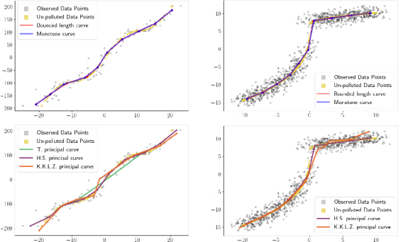
As a proof of concept, we generate 110 and 1000 observations of , where is monotone and is Gaussian noise. We set the domain to be either the set of measures supported on a monotone set or the set of measures supported on a curve with finite length. We solve problem (3) by adapting a generalized Lloyd algorithm. The self-consistency constraint is softly enforced via a penalty term in the objective function. For comparison, we also generated principal curves based on different definitions from [10], [15], and [21].333For the method proposed by [21], we only generate the curve using 110 data points, as we encounter overflow issues with larger sample sizes. The results are shown in Figure 3. The figures illustrate that the curve fitting method based on problem (3) performs reasonably well in capturing the underlying structure of the data compared to other principal curve methods.
Figure 3:
Principal curve fitting methods applied to 110 data points (Left) and 1000 monotone data points (Right). ”Monotone curve” and ”Bounded length curve” correspond to our solutions of problem (3) over the domain , defined as either the set of measures supported on a monotone set or those supported on a curve with finite length. These solutions are computed using a generalized Lloyd algorithm, where the self-consistency constraint is softly enforced via a penalty term in the objective function.
For comparison, we also present the results of fitting principal curves using the methods by Hastie-Stuetzle [10], Kégl-Krzyzak-Linder-Zeger [15], and Tibshirani [21].
3 The Kantorovich dominance relation
Despite its conceptual appeal, the learning problem with self consistency (3) (or equivalently (5)) has certain drawbacks: the convex order constraint is difficult to check, the problem may be unstable (recall Example 4), and the intersection of the certain natural domains with the set may be nearly empty, and thus not contain a reasonable solution (see, for example, the application in Section 4.4).
These challenges prompt us to introduce a weaker relation, the Kantorovich dominance relation, which still captures some aspects of the martingale property, while avoiding some of the computational and theoretical difficulties associated with the convex order relation.
Let denote the inner product. For , we say that is less than in the Kantorovich dominance relation (KDR), and write , if there is such that
(15)
Remark 4.
If , then there exists a martingale coupling such that
Therefore, the KDR is a relaxation of the convex order relation, capturing a weaker form of the martingale property. Precisely, for some coupling , the KDR requires only that is orthogonal to in .
A key part of the motivation for the Kantorovich dominance is that it arises as a sort of optimality condition for the relaxed problem (6) for a certain class of domains (see Theorem 4.9 below), analagously to the way that self consistency arises as an optimality condition for particularly simple domains (Proposition 2.2).
Remark 5.
If either or is centered, for (the product measure), we have
Since the image of the weakly continuous mapping over the connected set is itself connected, we conclude that (15) is equivalent to
(16)
(16) motivates the term Kantorovich dominance, as it shows that the ”Kantorovich cost” dominates (i.e., is greater than or equal to) the second moment of .
holds for all . In contrast, if (18) holds for , i.e., for . Exploring intermediate radii remains an open direction for further study.
We observe that the tail probability of is controlled by the second moment of if .
Lemma 3.1.
If , then we have
(19)
(19) easily follows from (17) and Markov’s inequality:
If we further assume that is compact and (e.g., with compact , where denotes the convex hull of ), then we obtain a stronger compactness.
Corollary 3.2.
is a precompact subset of with respect to the weak topology. If is compact, then is compact in both the weak and topologies.
Proof.
By Lemma 3.1 and Prokhorov’s theorem, is precompact in the weak topology. Since convergence is equivalent to weak convergence when is compact (see Remark 2.8 of [1]), and is closed, the result follows.
∎
However, is not necessarily compact in the topology, even if is compact. This motivates the consideration of the domain with a compact instead of .
Example 5.
Let denote the uniform probability measure over a sphere with radius centered at the origin. For , let and . The optimal coupling for sends radially to and to .
If is fixed, and let
,
it is straightforward to verify that inequality (17) still holds, and hence . This shows that the support of can be arbitrarily large (by letting ), and that the Kantorovich order relation is not equivalent to the convex order relation, even in one dimension.
This example also demonstrates that is not compact in , even if is compactly supported. If we let , as above, and , then as , converges weakly to the uniform probability measure over a sphere with radius and second moment . However, as , we have .
Although the KDR captures some properties of the convex order, it is not a partial order. Specifically, when , KDR violates the transitivity property.
Example 6.
Figure 4: An example showing that the KDR is not transitive and hence not a partial order.
Let , , and (see Figure 4). Clearly, and . Meanwhile, , , and . Thus, and by (17). However, since , we do not have .
4 Maximizing variance under the Kantorovich dominance relation
Throughout the sequel, we will assume that is a compact, convex set containing , unless stated otherwise. An example is . Let . Motivated by our earlier discussion, given a domain , we now study the following variance maximization problem:
(20)
Theorem 4.1.
i)
If is closed in the -metric and non-empty, then problem (20) admits a solution.
ii)
Let be any solution to (20). Then for any , we have:
Consequently, problem (20) exhibits a denoising property, meaning that as the noise in the measure decreases, the optimal solution tends to recover the original measure.
Proof.
i) Since is compact in the -metric by Corollary 3.2, and is -closed, it follows that is also -compact. The continuity of the variance functional with respect to the -metric guarantees that problem (20) admits a solution.
ii) The proof is similar to the proof of Theorem 2.4.
where the second inequality is by the KDR and the last inequality follows from the optimality of , which gives .
∎
4.1 Stability
Under a certain condition on , we now show problem (20) is stable, in contrast to (3), as shown in Example 4. The hypothesis we will impose on in the following definitions is quite weak; in particular, it is satisfied by all domains we have considered.
Definition 4.2.
Let . We say that is approachable from the interior with respect to if, for any with and , there exists a sequence such that and in (16) for all .
The class of domains that are closed under contractions serves as a key example of domains that can be approached from the interior.
Definition 4.3.
Let denote the dilation of by , i.e., when .
We say that is closed under contractions if for any and .
Lemma 4.4.
If is closed under contractions, then for any and with , there is a sequence such that and .
Proof.
If there is nothing to prove. If not, there exists some with . Let be an increasing sequence of positive numbers converging to and choose and , so that .
∎
The following result illustrates a stability property inherent to problem (20), where is not required to be compact.
Theorem 4.5.
Let and assume that is approachable from the interior w.r.t. . Let such that . Let be a solution to (20) with . If for some , then is a solution to (20) with .
Proof.
Consider first an arbitrary satisfying . By the strict inequality, for all large we have . By optimality of in (20) with , we have ; taking limits then yields .
Now consider any . Letting approximate such that , the above argument yields ; taking limits implies . As is arbitrary, optimality of follows.
∎
4.2 Conic domains and equivalence with the relaxed problem
We establish the equivalence between the problem (20) and the relaxed problem (6) under certain structural assumptions on . Notably, this result applies even when is not compact, ensuring the existence and stability of solutions in such cases as well.
Definition 4.6.
is called a cone if for any and . is called translation invariant if for any and , where .
Many of the domains we are interested in are cones and translation invariant, including those in Examples 2 and 3, as well as measures supported on lines and multivariate Gaussians as will be explored in Section 4.4 below. Note that the domain in Example 1 is not a cone.
Lemma 4.7.
Let , and let denote the translation of by . Among all translations , the one that minimizes the distance to is the one for which
(21)
Proof.
The distance between and is given by
where is an optimal transport plan between and . Differentiating with respect to and setting the derivative equal to zero gives .
Thus, the translation that minimizes the distance satisfies (21), as claimed.
∎
Lemma 4.8.
If is a cone, then for any and , the following equality holds:
(22)
If, in addition, is translation invariant, then must be centered; .
Proof.
By the KDR (16), for any and for any corresponding optimal coupling , we have the inequality:
(23)
Suppose this inequality is strict for some . As is a cone, for any . Let be the corresponding coupling of and .
If the inequality (23) is strict, there exists a such that:
meaning that . However, the variance of exceeds that of (unless , in which case the result is trivial), contradicting the optimality of . We conclude that the inequality (23) must hold with equality for any optimal and .
To see if is translation invariant, let and be defined as in Lemma 4.7. Setting a coupling of and ,
shows . With this, implies is also optimal. Now yields strict inequality above, which contradicts (22). We conclude .
∎
We can now extend the solution existence result for the problem (20) when .
Theorem 4.9.
Let , and let be a cone. Suppose that is either translation invariant or . Then, the problem (20) with is equivalent to the relaxed problem (6), meaning that both formulations have the same set of solutions.
Proof.
For any and , we claim
(24)
that is, . To see this, for any , consider a rescaling factor that solves
The optimal scaling is attained at:
Since for the optimal (no rescaling improves the objective function), (24) follows.
Next, by the assumption on and Lemma 4.7, . This and (24) imply
(25)
where we have used Lemma 4.8 to remove in (25). This shows any solution to the relaxed problem (6) is also a solution to (20) with . Conversely, if solves (20), the equality of values (25) and Lemma 4.8 imply that solves (6), completing the proof.
∎
4.3 Weak optimizer closedness and equivalence to the problem with self-consistency
We have shown that for appropriate domains, the problem (20) is equivalent to the fully relaxed problem (6). We now consider when (20) is equivalent to the problem with the full self-consistency condition (3).
Recall the centering map from Definition 2.1.
Definition 4.10.
Let and .
We say that is closed under weak optimizers if, for any that solves (20), there exists such that
(26)
For instance, the domains and in Example 3 are closed under weak optimizers.
Theorem 4.11.
If is closed under weak optimizers, then every optimizer for the problem (20) satisfies , and consequently, solves the original problem (5).
Proof.
Assume that solves (20), so there exists satisfying (26). Since is a martingale measure, we have
Now, as the barycenter minimizes the expected squared distance, we have the inequality
with strict inequality if . After canceling , we get
with strict inequality if . Adding this to the previous inequality gives
The optimality of implies equality. Hence , which implies .
∎
4.4 Relationship with principal component analysis
In this section, we explore the relationship between our formulation (20) and principal component analysis (PCA). Let denote the set of all -dimensional subspaces of . Consider the following cone domain:
Let denote the orthogonal projection map onto a subspace of .
Lemma 4.12.
Any solving the problem , where , is the orthogonal projection of onto some .
Proof.
Theorem 4.9 shows the problem is equivalent to the relaxed problem . Noting , where , we can decompose the relaxed problem as . The lemma follows by the fact that the projection is the unique minimizer of .
∎
Lemma 4.12 reveals that PCA can be viewed as a particular case of problem (20) with the domain . Specifically, the first principal component is defined as the direction that maximizes the variance of the projected data. Lemma 4.12 demonstrates that the projected data satisfies the variance maximization problem under the Kantorovich dominance constraint.
We now consider the following version of the PCA in [6, Section 3.3]. Consider the model
(27)
where is an -dimensional Gaussian vector of latent factors, is an unknown factor loading matrix of rank , and represents random noise that is independent of and cannot be explained by the latent factor. Without loss of generality, assume that , where the columns of form an orthonormal set, and is a diagonal matrix with .
Let . We now focus on solving the problem (20) over the following cone domain
(28)
Note that the problem (20) remains equivalent to the relaxed problem (6), by Theorem 4.9.
Theorem 4.13.
Let where , . Then for all , with in (28), and for any with ,
(29)
where is an estimator of the noise variance .
Remark 7.
(29) indicates that the optimization problem can recover as the empirical distribution converges to the population distribution .
This result cannot hold if the full convex order constraint is imposed. In many practical cases, such as when is discrete (e.g., is an empirical measure sampled from ), the convex order condition fails for any Gaussian unless . As a result, the domain reduces to if is centered; otherwise, it is empty since .
Let and as in (28). If , then and . If , then as well.
Proof.
Assume that in the diagonal of . Since implies is bounded, the sequences and are precompact. For any subsequences of and of converging to and , respectively, define . Then, implies , which ensures
for where is the th column of (notice this yields if ),
and , i.e., for . Consequently, . The arbitrariness of the subsequence establishes the lemma. The more general case, , can be similarly proven by taking into account the multiplicity of the singular values .
∎
is compact by Lemma 4.14, and
. Notice the unique solution to is ,
since , and the -projection of onto is clearly .
Then for any , Lemma 4.14 and Theorem 4.5 give . Then since and , Lemma 4.15 gives , and . This with implies , yielding .
∎
5 Numerical examples
We provide examples of numerically solving the KDR problem with and three closely related discrete curve domains.
5.1 Curves with bounded length
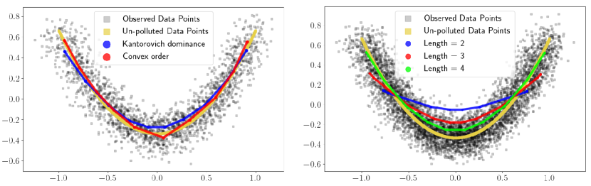
Figure 5: Left: Optimal measure under the Kantorovich dominance and the convex order for 2000 data points. Right: Optimal measure under the Kantorovich dominance for 5000 data points.
Our first example considers the following domain
where represents the length of the discrete curve . Due to the length bound, is not a cone.
To address the bound, we transform the constrained optimization problem into an unconstrained form by introducing a Lagrangian with multipliers that correspond to each constraint. Details are given in Section B of the Supplementary Material. The method employs gradient ascent to update the position and weight , while applying gradient descent to update the Lagrange multipliers iteratively.
It is possible to numerically solve problem (3), particularly the martingale constraint, using gradient descent. However, this approach involves optimizing over a larger set of unknowns for the coupling rather than focusing on alone, which leads to increased memory requirements for storing variables, greater computational demand for calculating gradients, and potentially longer convergence times. In contrast, although calculating the coupling is still required to compute the distance for the KDR problem, it can be done efficiently using the Sinkhorn algorithm [7], [5], which is known for its speed and computational efficiency.
To illustrate our example, we consider as a discrete measure, defined over either or points, where , with being a one-dimensional variable uniformly distributed over , and representing Gaussian noise. The initial measure is supported on points, which are initialized along the first principal component of .
Using the proposed method, we optimize the location and the weight .
In the case of data points, we set the length bound and the left side of Figure 5 illustrates the optimal under both the Kantorovich dominance relation and the convex order relation. For the case with 5000 data points, an out-of-memory error occurred when attempting to compute the optimal measure under the convex order. Therefore, we present only the optimal measure under the KDR, with and , as shown in the right side of Figure 5.444The Python code for Example 5.1 is available at Joshua’s Github here…
Further improvement in performance is achieved in the case of cone domains, as enabled by the following result.
Proposition 5.1.
Assume that is a cone and translation invariant. Then, solving the problem (20) with is equivalent to solving the following problem:
(30)
Proof.
By Theorem 4.9, the problem (20) is equivalent to the problem ,
which, by Lemma 4.8 and equation (24) in the proof of Theorem 4.9, is also equivalent to:
(31)
We will show that any optimizer for (31) induces a solution to (30), and conversely. For , and , define and . Then for any feasible pair for (30) and for (31) with and ,
(32)
(33)
where so that , while is the unique constant yielding the second equality in (33). This shows is feasible for (30) and for (31), and moreover, if , then for any optimal pair for (30) and for (31), we have
(34)
since for any optimal pair for (30), the constraint must be tight, meaning that the inequality in (33) is satisfied as an equality. Then (34), with (32) and (33), shows that for any optimal for (30), its scaling is optimal for (31), and conversely, for any optimal for (31), is optimal for (30). Finally, the proof also shows if and only if , in which case serves as the trivial solution to both problems.
∎
In the following, we apply this result to solve two examples with cone domains555Source code for examples 5.2 and 5.3 are available at https://github.com/souza-m/data-denoising.. In both cases, we use fixed weights for , specifically , to approximate a dataset of distributed along a step-shaped curve with added noise.
5.2 Curves with bounded length-to-standard-deviation ratio
Here we consider the following modification of the domain :
where represents the standard deviation of . Thus, the bound is now imposed on the ratio between the length and the standard deviation. Since rescaling does not change the ratio , we see that is a cone.
For each value of , we set points and linearly connect them. Figure 6 illustrates the resulting curves. We can see that as increases, so does the curve length. Supplementary Material C describes the alternating numerical steps for the solution.
Figure 6: Left: Curves with bounded length-standard deviation ratios. Right: Curves with bounded curvatures. Curves are formed by connecting points using straight lines.
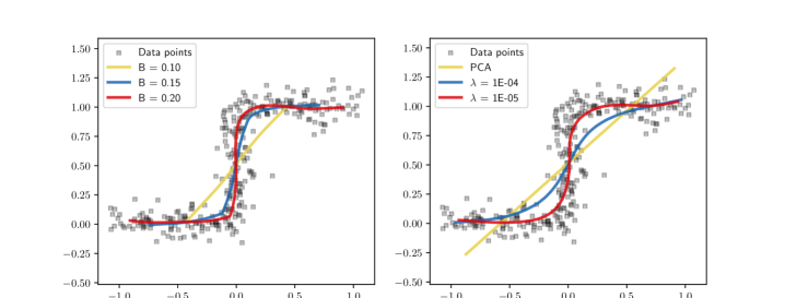
5.3 Curves with bounded curvature
Our last example considers a domain given by
where represents the total curvature, with being the angle between segments and . is a cone since the angles do not change with scaling of , and by Lemma 4.12, corresponds to the problem of finding the first principal direction.
In the numerical computation, the curvature constraint is handled indirectly via penalization and solved using an alternating method, as detailed in the Supplementary Material C. For each curvature penalty parameter , we set points and connect them linearly to form curves in Figure 6, where the first principal direction is also included for reference.
The examples in this section demonstrate that the proposed method can efficiently compute the optimal measure under the Kantorovich dominance with large datasets.
{acks}
[Acknowledgments]
B.P. is pleased to acknowledge the support of Natural Sciences and Engineering Research Council of Canada Discovery Grant numbers 04658-2018 and 04864-2024. The work of J.H. and M.S. is in partial fulfillment of their doctoral degrees.
References
[1]
Luigi Ambrosio and Nicola Gigli.
A User’s Guide to Optimal Transport, pages 1–155.
Springer Berlin Heidelberg, Berlin, Heidelberg, 2013.
[2]
Mathias Beiglböck and Nicolas Juillet.
On a problem of optimal transport under marginal martingale
constraints.
The Annals of Probability, 44(1):42 – 106, 2016.
[3]
Stephen Boyd and Lieven Vandenberghe.
Convex optimization.
Cambridge university press, 2004.
[4]
Martin Brückerhoff and Nicolas Juillet.
Instability of martingale optimal transport in dimension .
Electronic Communications in Probability, 27:1–10, 2022.
[5]
Guillaume Carlier.
On the linear convergence of the multimarginal sinkhorn algorithm.
SIAM Journal on Optimization, 32(2):786–794, 2022.
[6]
Yuxin Chen, Yuejie Chi, Jianqing Fan, and Cong Ma.
Spectral methods for data science: A statistical perspective.
Foundations and Trends® in Machine Learning,
14(5):566–806, 2021.
[7]
Marco Cuturi.
Sinkhorn distances: Lightspeed computation of optimal transport.
In Advances in Neural Information Processing Systems,
volume 26. Curran Associates, Inc., 2013.
[8]
Tom Duchamp and Werner Stuetzle.
Extremal properties of principal curves in the plane.
The Annals of Statistics, 24(4):1511 – 1520, 1996.
[9]
Michael Greenacre, Patrick JF Groenen, Trevor Hastie, Alfonso Iodice d’Enza,
Angelos Markos, and Elena Tuzhilina.
Principal component analysis.
Nature Reviews Methods Primers, 2(1):100, 2022.
[10]
Trevor Hastie and Werner Stuetzle.
Principal curves.
Journal of the American Statistical Association,
84(406):502–516, 1989.
[11]
Pierre Henry-Labordère.
Model-free hedging: A martingale optimal transport viewpoint.
Chapman and Hall/CRC, 2017.
[12]
I.T. Jolliffe.
Principal Component Analysis.
Springer Series in Statistics. Springer, 2nd ed. edition, 2002.
[13]
Seungwoo Kang and Hee-Seok Oh.
Probabilistic principal curves on riemannian manifolds.
IEEE Transactions on Pattern Analysis and Machine Intelligence,
2024.
[14]
Tapas Kanungo, David Mount, Nathan Netanyahu, Christine Piatko, Ruth Silverman,
and Angela Wu.
An efficient k-means clustering algorithm: Analysis and
implementation.
IEEE transactions on pattern analysis and machine intelligence,
24(7):881–892, 2002.
[15]
Balázs Kégl, Adam Krzyzak, Tamás Linder, and Kenneth Zeger.
Learning and design of principal curves.
IEEE transactions on pattern analysis and machine intelligence,
22(3):281–297, 2000.
[16]
Dmitry Kramkov and Yan Xu.
An optimal transport problem with backward martingale constraints
motivated by insider trading.
The Annals of Applied Probability, 32(1):294–326, 2022.
[17]
Jongmin Lee, Jang-Hyun Kim, and Hee-Seok Oh.
Spherical principal curves.
IEEE Transactions on Pattern Analysis and Machine Intelligence,
43(6):2165–2171, 2020.
[18]
Stuart Lloyd.
Least squares quantization in pcm.
IEEE transactions on information theory, 28(2):129–137, 1982.
[19]
George J. Minty.
Monotone (nonlinear) operators in Hilbert space.
Duke Math. J., 29:341–346, 1962.
[20]
Filippo Santambrogio.
Optimal transport for applied mathematicians.
Birkäuser, NY, 55(58-63):94, 2015.
[21]
Robert Tibshirani.
Principal curves revisited.
Statistics and computing, 2:183–190, 1992.
[22]
Cédric Villani.
Topics in Optimal Transportation.
Number 58. American Mathematical Soc., 2003.
[23]
Johannes Wiesel and Erica Zhang.
An optimal transport-based characterization of convex order.
Dependence Modeling, 11(1):20230102, 2023.
{supplement}\stitle
A: Solution comparison between the problem (3) and the problem studied in [16].
We present an example which shows that the optimal measure for problem (1.2) in [16] is not an optimal measure for our problem (3).
We define the measure and as follows:
We define the martingale coupling between and as follows:
while the martingale coupling between and as follows:
For , , let be the cost function considered in [16]. It is straightforward to check that for any ,
(35)
By [16, Theorem 2.2], (35) shows that is the optimal coupling for their problem.
On the other hand, it is also easy to check that provide a better coupling for our problem (3), showing the optimal measure for problem (1.2) in [16] is not the optimal measure for (3).
{supplement}\stitle
B: Computational details for Section 5.1.
The Lagrangian we maximize for the example in Section 5.1 is the following:
where is the variance of , is the Lagrange multiplier for the probability constraint , enforces , enforces the length constraint , and enforces the Kantorovich dominance constraint.
The complementary slackness condition for each constraint ensures that the Lagrange multipliers only contribute when their respective constraints are active. Specifically:
Let be an optimal coupling corresponding to . The gradients with respect to the location and weight are computed as follows.
Gradient with respect to :
Gradient with respect to :
The optimal transport plan with marginal using current and and given . is calculated using the Sinkhorn algorithm for efficiency.
The multipliers are updated using projected gradient descent to satisfy the KKT conditions, with non-negativity of the multipliers enforced by projecting onto the feasible region. Specifically, each update step is given by:
The projection operator ensures that and remain non-negative, in line with the KKT requirements.
{supplement}\stitle
C: Computational details for Sections 5.2 and 5.3.
To approximate a solution to (30), we propose an alternating procedure that splits the problem into two subproblems, optimizing with respect to each variable separately. The variables are , where each , and . These examples use the constant weight on the points of , that is, we set . represents a transport plan / coupling between the variable and the data , subject to the marginal constraints for all , and for all .
The optimization begins with an initial set satisfying the constraints and and the domain constraint (e.g., the set of PCA projections in both examples). At each iteration , we perform the following two steps, repeating until convergence. The final output is the pair , where is rescaled by the factor given in (34).
Step 1. Given , find that solves
Step 2. Given , set and find that solves
In Step 1, note that the constraints on are satisfied by construction, since the marginal condition imposes and . Thus, the problem falls into the class of traditional optimal transport with fixed marginals. To solve it, in both examples we apply the Sinkhorn method, as noted in Subsection 5.1. Then to solve Step 2 in Subsection 5.2, we explicitly state the domain constraint on as follows:
Since the second constraint is clearly binding, together with the third constraints it implies that any solution to the above satisfies the domain constraint . We convert this problem into a second-order conic program, which can be solved efficiently by interior point methods – see [3] for an overview. To do that, we define the variable to be optimized as
where the superscript in denotes the dimensional component and is an auxiliary variable. The second-moment constraint on is replaced by the equivalent
The constraints are equivalently rewritten as
We solve the problem in this format using Python and CVXOPT package.
In Step 2 of Subsection 5.3, we replace the domain constraint by a linear penalization together with another, inner iteration loop, as follows. Call for , and for . Notice that . At iteration , the problem is solved for
defined as
where . The penalized problem is written as
where for some penalization multiplier . We solve it through the Lagrangian
The first derivatives are
We can assume that the second-moment condition is binding and ,
since otherwise it would be possible to increase the objective function.
The first order conditions imply
Replacing and gives
as a function of . Finally, we update partially at each iteration, as where solves the problem for . The loop stops when the sequence converges to a fixed point ,
and we get