Wolfpack Adversarial Attack for Robust Multi-Agent Reinforcement Learning

Abstract

Traditional robust methods in multi-agent reinforcement learning (MARL) often struggle against coordinated adversarial attacks in cooperative scenarios. To address this limitation, we propose the Wolfpack Adversarial Attack framework, inspired by wolf hunting strategies, which targets an initial agent and its assisting agents to disrupt cooperation. Additionally, we introduce the Wolfpack-Adversarial Learning for MARL (WALL) framework, which trains robust MARL policies to defend against the proposed Wolfpack attack by fostering system-wide collaboration. Experimental results underscore the devastating impact of the Wolfpack attack and the significant robustness improvements achieved by WALL.

ecases  $\displaystyle{##}$ $\displaystyle{##}$ {. ecases*  $\displaystyle{##}$ ## {.

^∗

1 Introduction

Multi-agent Reinforcement Learning (MARL) has gained attention for solving complex problems requiring agent cooperation (Oroojlooy & Hajinezhad, 2023) and competition, such as drone control (Yun et al., 2022), autonomous navigation (Chen et al., 2023), robotics (Orr & Dutta, 2023), and energy management (Jendoubi & Bouffard, 2023). To handle partially observable environments, the Centralized Training and Decentralized Execution (CTDE) framework (Oliehoek et al., 2008) trains a global value function centrally while agents execute policies based on local observations. Notable credit-assignment methods in CTDE include Value Decomposition Networks (VDN) (Sunehag et al., 2017), QMIX (Rashid et al., 2020), which satisfies the Individual-Global-Max (IGM) condition ensuring that optimal joint actions align with positive gradients in global and individual value functions, and QPLEX (Wang et al., 2020b), which encodes IGM into its architecture. However, CTDE methods face challenges from exploration inefficiencies (Mahajan et al., 2019; Jo et al., 2024) and mismatches between training and deployment environments, leading to unexpected agent behaviors and degraded performance (Moos et al., 2022; Guo et al., 2022). Thus, enhancing the robustness of CTDE remains a critical research focus.

To improve learning robustness, single-agent RL methods have explored strategies based on game theory (Yu et al., 2021), such as max-min approaches and adversarial learning (Goodfellow et al., 2014; Huang et al., 2017; Pattanaik et al., 2017; Pinto et al., 2017). In multi-agent systems, simultaneous agent interactions introduce additional uncertainties (Zhang et al., 2021b). To address this, methods like perturbing local observations (Lin et al., 2020), training with adversarial policies for Nash equilibrium (Li et al., 2023a), adversarial value decomposition (Phan et al., 2021), and attacking inter-agent communication (Xue et al., 2021) have been proposed. However, these approaches often target a single agent per attack, overlooking interdependencies in cooperative MARL, making them vulnerable to scenarios where multiple agents are attacked simultaneously.

To overcome the vulnerabilities posed by coordinated adversarial attacks in MARL, we propose the Wolfpack adversarial attack framework, inspired by wolf hunting strategies. This approach disrupts inter-agent cooperation by targeting a single agent and subsequently attacking the group of agents assisting the initially targeted agent, resulting in more devastating impacts. Experimental results reveal that traditional robust MARL methods are highly susceptible to such coordinated attacks, underscoring the need for new defense mechanisms. In response, we also introduce the Wolfpack-Adversarial Learning for MARL (WALL) framework, a robust policy training approach specifically designed to counter the Wolfpack Adversarial Attack. By fostering system-wide collaboration and avoiding reliance on specific agent subsets, WALL enables agents to defend effectively against coordinated attacks. Experimental evaluations demonstrate that WALL significantly improves robustness compared to existing methods while maintaining high performance under a wide range of adversarial attack scenarios. The key contributions of this paper in constructing the Wolfpack Adversarial Attack are summarized as follows:

• A novel MARL attack strategy, Wolfpack Adversarial Attack, is introduced, targeting multiple agents simultaneously to foster stronger and more resilient agent cooperation during policy training.

• The follow-up agent group selection method is proposed to target agents with significant behavioral adjustments to an initial attack, enabling subsequent sequential attacks and amplifying their overall impact.

• A planner-based attacking step selector predicts future $Q$-value reductions caused by the attack, enabling the selection of critical time steps to maximize impact and improve learning robustness.

2 Related Works

Robust MARL Strategies: Recent research has focused on robust MARL to address unexpected changes in multi-agent environments. Max-min optimization (Chinchuluun et al., 2008; Han & Sung, 2021) has been applied to traditional MARL algorithms for robust learning (Li et al., 2019; Wang et al., 2022). Robust Nash equilibrium has been redefined to better suit multi-agent systems (Zhang et al., 2020b; Li et al., 2023a). Regularization-based approaches have also been explored to improve MARL robustness (Lin et al., 2020; Li et al., 2023b; Wang et al., 2023; Bukharin et al., 2024), alongside distributional reinforcement learning methods to manage uncertainties (Li et al., 2020; Xu et al., 2021; Du et al., 2024; Geng et al., 2024).

Adversarial Attacks for Resilient RL: To strengthen RL, numerous studies have explored adversarial learning to train policies under worst-case scenarios (Pattanaik et al., 2017; Tessler et al., 2019; Pinto et al., 2017; Chae et al., 2022). These attacks introduce perturbations to various MDP components, including state (Zhang et al., 2020a, 2021a; Everett et al., 2021; Li et al., 2023c; Qiaoben et al., 2024), action (Tan et al., 2020; Lee et al., 2021; Liu et al., 2024), and reward (Wang et al., 2020a; Zhang et al., 2020c; Rakhsha et al., 2021; Xu et al., 2022; Cai et al., 2023; Bouhaddi & Adi, 2023; Xu et al., 2024; Bouhaddi & Adi, 2024). Adversarial attacks have recently been extended to multi-agent setups, introducing uncertainties to state or observation (Han et al., 2022; He et al., 2023; Zhang et al., 2023; Zhou et al., 2023), actions (Yuan et al., 2023), and rewards (Kardeş et al., 2011). Further research has applied adversarial attacks to value decomposition frameworks (Phan et al., 2021), selected critical agents for targeted attacks (Yuan et al., 2023; Zhou et al., 2024), and analyzed their effects on inter-agent communication (Xue et al., 2021; Tu et al., 2021; Sun et al., 2023; Yuan et al., 2024).

Model-based Frameworks for Robust RL: Model-based methods have been extensively studied to enhance RL robustness (Berkenkamp et al., 2017; Panaganti & Kalathil, 2021; Curi et al., 2021; Clavier et al., 2023; Shi & Chi, 2024; Ramesh et al., 2024), including adversarial extensions (Wang et al., 2020c; Kobayashi, 2024). Transition models have been leveraged to improve robustness (Mankowitz et al., 2019; Ye et al., 2024; Herremans et al., 2024), and offline setups have been explored for robust training (Rigter et al., 2022; Bhardwaj et al., 2024). In multi-agent systems, model-based approaches address challenges like constructing worst-case sets (Shi et al., 2024) and managing transition kernel uncertainty (He et al., 2022).

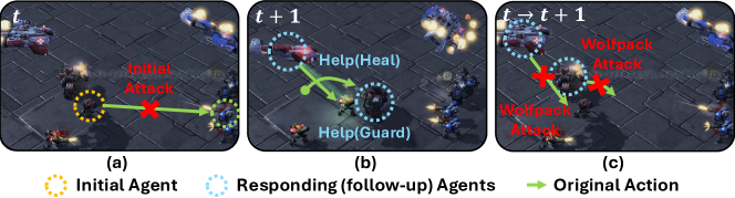
Figure 1: Visualization of Wolfpack attack strategy during combat in the Starcraft II environment: (a) The initial agent is attacked, disrupting its original action (b) Responding (follow-up) agents to help the initially attacked agent and (c) Wolfpack adversarial attack that disrupts help actions of follow-up agents.

3 Background

3.1 Dec-POMDP and Value-based CTDE Setup

A fully cooperative multi-agent environment is modeled as a decentralized partially observable Markov decision process (Dec-POMDP) (Oliehoek et al., 2016), defined by the tuple $\mathcal{M}=\langle\mathcal{N},\mathcal{S},\mathcal{A},P,\Omega,O,R,\gamma\rangle$. $\mathcal{N}={1,\ldots,n}$ is the set of agents, $\mathcal{S}$ the global state space, $\mathcal{A}=\mathcal{A}^{1}\times\cdots\times\mathcal{A}^{n}$ the joint action space, $P$ the state transition probability, $\Omega$ the observation space, $R$ the reward function, and $\gamma\in[0,1)$ the discount factor. At time $t$, each agent $i$ observes $o_{t}^{i}=O(s_{t},i)\in\Omega$ and takes action $a_{t}^{i}\in\mathcal{A}^{i}$ based on its individual policy $\pi^{i}(\cdot|\tau_{t}^{i})$, where $\tau_{t}^{i}$ is the agent’s trajectory up to $t$. The joint action $\mathbf{a}_{t}=\langle a_{t}^{1},\ldots,a_{t}^{n}\rangle$ sampled from the joint policy $\mathbf{\pi}:=\langle\pi^{1},\cdots,\pi^{n}\rangle$ leads to the next state $s_{t+1}\sim P(\cdot|s_{t},\mathbf{a}_{t})$ and reward $r_{t}:=R(s_{t},\mathbf{a}_{t})$. MARL aims to find the optimal joint policy that maximizes $\sum_{t=0}^{\infty}\gamma^{t}r_{t}$. As noted, this paper adopts the centralized training with decentralized execution (CTDE) setup, where the joint value $Q^{tot}(s_{t},\mathbf{a}_{t})$ is learned using temporal-difference (TD) learning. Through credit assignment, individual value functions $Q^{i}(\tau_{t}^{i},a_{t}^{i})$ are learned, guiding individual policies $\pi^{i}$ to select actions that maximize $Q^{i}$, i.e., $\pi^{i}:=\arg\max_{a_{t}^{i}\in\mathcal{A}^{i}}Q^{i}(\tau_{t}^{i},\cdot)$.

3.2 Robust MARL with Adversarial Attack Policy

Among various methods for robust learning in MARL, Yuan et al. (2023) defined an adversarial attack policy $\pi_{\mathrm{adv}}$ and implemented robust MARL by training multi-agent policies to defend against attacks executed by $\pi_{\mathrm{adv}}:\mathcal{S}\times\mathcal{A}\times\mathbb{N}\rightarrow\mathcal{A}$. A cooperative MARL environment with an adversarial policy $\pi_{\mathrm{adv}}$ can be described as a Limited Policy Adversary Dec-POMDP (LPA-Dec-POMDP) $\tilde{\mathcal{M}}$, defined as follows:

Definition 3.1 (Limited Policy Adversary Dec-POMDP).

Given a Dec-POMDP $\mathcal{M}$ and a fixed adversarial policy $\pi_{\mathrm{adv}}$, we define a Limited Policy Adversary Dec-POMDP (LPA-Dec-POMDP) $\tilde{\mathcal{M}}=\langle\mathcal{N},\mathcal{S},\mathcal{A},P,K,\Omega,O,R,\gamma\rangle$, where $K$ is the maximum number of attacks, $\pi_{\mathrm{adv}}(\cdot|s_{t},\mathbf{a}_{t},k_{t})$ executes joint action $\tilde{\mathbf{a}}_{t}$ to disrupt the original action $\mathbf{a}_{t}$ chosen by $\pi$, and $k_{t}\leq K$ indicates the number of remaining attacks.

Here, if $\pi_{\mathrm{adv}}$ selects an attack action $\tilde{\mathbf{a}}_{t}$ different from the original action $\mathbf{a}_{t}$, the remaining number of attacks $k_{t}$ decreases by 1. Once $k_{t}$ reaches 0, no further attacks can be performed. In this framework, Yuan et al. (2023) also demonstrated that the LPA-Dec-POMDP can be represented as another Dec-POMDP induced by $\pi_{\mathrm{adv}}$, with the convergence of the optimal policy $\pi^{*}$ under $\tilde{\mathcal{M}}$ guaranteed. In particular, it considers an adversarial attack targeting a chosen agent $i$ by minimizing its individual value function $Q^{i}$, as proposed by (Pattanaik et al., 2017), i.e., $\tilde{a}_{t}^{i}=\arg\min_{a\in\mathcal{A}^{i}}Q^{i}(\tau_{t}^{i},a)$. Additionally, to enhance the attack’s effectiveness, an evolutionary generation of attacker (EGA) approach is proposed, which combines multiple adversarial policies.

4 Methodology

4.1 Motivation of Wolfpack Attack Strategy

Existing adversarial attackers typically target only a single agent per attack, without coordination or relationships between successive attacks. In a cooperative MARL setup, such simplistic attacks enable non-targeted agents to learn effective policies to counteract the attack. However, we observe that policies trained under these conditions are vulnerable to coordinated attacks. As illustrated in Fig. 1(a), a single agent is attacked at time $t$. In Fig. 1(b), at the next step $t+1$, responding agents adjust their actions, such as healing or moving to guard, to protect the initially attacked agent. In contrast, Fig. 1(c) demonstrates a coordinated attack strategy that targets the agents responding to the initial attack. Such coordinated attacks render the learned policy ineffective, preventing it from countering the attacks entirely. This highlights that coordinated attacks are far more detrimental than existing attack methods, and current robust policies fail to defend effectively against them.

As depicted in Fig. 1(c), targeting agents that respond to an initial attack aligns with the Wolfpack attack strategy, a tactic widely employed in traditional military operations, as discussed in Section 1. To adapt this concept to a cooperative multi-agent setup, we define a Wolfpack adversarial attack as a coordinated strategy where one agent is attacked initially, followed by targeting the group of follow-up agents that respond to defend against the initial attack, as shown in Fig. 1(c). Leveraging this approach, we aim to develop robust policies capable of effectively countering Wolfpack adversarial attack, thereby significantly enhancing the overall resilience of the learning process.

4.2 Wolfpack Adversarial Attack

In this section, we formally propose the Wolfpack adversarial attack, as introduced in the previous sections. The Wolfpack attack consists of two components: initial attacks, where a single agent is targeted at a specific time step $t_{\mathrm{init}}$, and follow-up group attacks, where the group of agents responding to the initial attack is selected and targeted over the subsequent steps $t_{\mathrm{init}}+1,\cdots,t_{\mathrm{init}}+t_{\mathrm{WP}}$. Over the course of an episode, a maximum of $K_{\mathrm{WP}}$ Wolfpack attacks can be executed. Consequently, the total number of attack steps is given by $K=K_{\mathrm{WP}}\times(t_{\mathrm{WP}}+1)$. The Wolfpack adversarial attacker $\pi_{\mathrm{adv}}^{\mathrm{WP}}$ can then be defined as follows:

Definition 4.1 (Wolfpack Adversarial Attacker).

A Wolfpack adversarial attacker $\pi_{\mathrm{adv}}^{\mathrm{WP}}:\mathcal{S}\times\mathcal{A}\times\mathbb{N}\rightarrow\mathcal{A}$ is defined as $\tilde{\mathbf{a}}_{t}=\pi_{\mathrm{adv}}^{\mathrm{WP}}(s_{t},\mathbf{a}_{t},k_{t})$, where $\tilde{a}_{t}^{i}=\arg\min_{a_{t}^{i}\in\mathcal{A}^{i}}Q^{tot}(s_{t},a_{t}^{i},\mathbf{a}_{t}^{-i})$ for all $i\in\mathcal{N}_{t,\mathrm{attack}}$, and $\tilde{a}_{t}^{i}=a_{t}^{i}$ otherwise. Here, $\mathbf{a}_{t}^{-i}$ represents the joint actions of all agents excluding the $i$-th agent, and $\mathcal{N}_{t,\mathrm{attack}}$ denotes the set of agents targeted for adversarial attack, defined as

$$\mathcal{N}_{t,\mathrm{attack}}=\ecases*\emptyset&ifk_{t}=0,\\ \{i\}elseift=t_{\mathrm{init}},i\sim\mathrm{Unif}(\mathcal{N}),\\ \mathcal{N}_{\mathrm{follow-up}}elseift=t_{\mathrm{init}}+1,\cdots,t_{\mathrm{init}}+t_{\mathrm{WP}},\\ \emptyset otherwise,$$

where $\mathrm{Unif}(\cdot)$ is the Uniform distribution, $\mathcal{N}_{\mathrm{follow-up}}:=\{i_{1},\cdots,i_{m}\}\subset\mathcal{N}$ is the group of agents selected for follow-up attack, and $m$ is the number of follow-up agents.

Here, note that $k_{t}$ decreases by $1$ for every attack step such that $\tilde{\mathbf{a}}_{t}\neq\mathbf{a}_{t}$, as in the ordinary adversarial attack policy, and the total value function $Q^{tot}$ is used for the attack instead of $Q^{i}$. The proposed Wolfpack adversarial attacker $\pi_{\mathrm{adv}}^{\mathrm{WP}}$ is a special case of the adversarial policy defined in Definition 3.1. Consequently, the proposed attacker forms an LPA-Dec-POMDP $\tilde{\mathcal{M}}$ induced by $\pi_{\mathrm{adv}}^{\mathrm{WP}}$, and as demonstrated in Yuan et al. (2023), the convergence of MARL within the LPA-Dec-POMDP can be guaranteed. The proposed Wolfpack attack involves two key issues: how to design the group of follow-up agents $\mathcal{N}_{\mathrm{follow-up}}$ and when to select $t_{\mathrm{init}}$. The following sections address these aspects in detail.

4.3 Follow-up Agent Group Selection Method

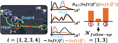
Figure 2: Visualization of Follow-Up Agent Group Selection Method: Agent $4$ is initially attacked, and the $m$ agents exhibiting the largest changes in $Q^{i}$ are selected from $\{1,2,3\}$ $(m=2)$.

In the Wolfpack adversarial attacker, we aim to identify the follow-up agent group $\mathcal{N}_{\mathrm{follow-up}}$ that actively responds to the initial attack $\pi_{\mathrm{adv}}^{\mathrm{WP}}(s_{t_{\mathrm{init}}},\mathbf{a}_{t_{\mathrm{init}}},k_{t_{\mathrm{init}}})$ and target them in subsequent steps. To do this, we define the difference between the $Q$-functions from the original action and the initial attack at time $t$ as:

$$\Delta Q_{t}^{tot}=Q^{tot}(s_{t},\mathbf{a}_{t})-Q^{tot}(s_{t},\tilde{\mathbf{a}}_{t}),$$

where $\Delta Q_{t}^{tot}\geq 0$ for all $t$ such that $\mathcal{N}_{t,\mathrm{attack}}\neq\emptyset$, because $\tilde{\mathbf{a}}t$ minimizes $Q^{tot}$ for the agent indices selected by $\pi_{\mathrm{adv}}^{\mathrm{WP}}$. Assuming the $i$-th agent is the target of the initial attack, updating $Q^{tot}$ based on $\Delta Q_{t_{\mathrm{init}}}^{tot}$ adjusts each agent’s individual value function $Q^{j}$ to increase $Q^{tot}$ for all $j\neq i\in\mathcal{N}$, in accordance with the credit assignment principle in CTDE algorithms (Sunehag et al., 2017; Rashid et al., 2020), as shown below:

$$\tilde{Q}^{i}(\tau_{t_{\mathrm{init}}}^{i},\cdot),=Q^{i}(\tau_{t_{\mathrm{init}}}^{i},\cdot)-\alpha_{\mathrm{lr}}\left.{\partial\Delta Q_{t_{\mathrm{init}}}^{tot}\over\partial Q^{i}(\tau_{t_{\mathrm{init}}}^{i},\mathbf{a})}\right|_{\mathbf{a}=\tilde{\mathbf{a}}_{t_{\mathrm{init}}}},$$ (1)

where $\alpha_{\mathrm{lr}}$ is the learning rate. As agents select actions based on $Q^{j}$, changes in $Q^{j}$ indicate adjustments in their policies in response to the initial attack. Agents with the largest changes in $Q^{j}$ are identified as follow-up agents, while the $i$-th agent is excluded as it is already under attack and cannot respond immediately.

To identify the follow-up agent group, the updated $\tilde{Q}^{j}$ and original $Q^{j}$ are transformed into distributions using the Softmax function $\mathrm{Soft}()$. This transformation softens the deterministic policy $\pi^{j}$, which directly selects an action to maximize $Q^{j}$, making distributional differences easier to compute. The follow-up agent group is determined by selecting the $m$ agents that maximize the Kullback-Leibler (KL) divergence $D_{\mathrm{KL}}$ between these distributions:

$$\mathcal{N}_{\mathrm{follow-up}} =\underset{\mathcal{N}^{\prime}\subset\mathcal{N},|\mathcal{N}^{\prime}|=m,j\in\mathcal{N}^{\prime},j\neq i}{\arg\max}\sum_{j}D_{\mathrm{KL}}\big{(}$$ (2)

$$\mathrm{Soft}(Q^{j}(\tau_{t_{\mathrm{init}}}^{j},\cdot))||\mathrm{Soft}(\tilde{Q}^{j}(\tau_{t_{\mathrm{init}}}^{j},\cdot))\big{)}.$$

Using the proposed method, the follow-up agent group is identified as the agents whose policy distributions experience the most significant changes following the initial attack. Fig. 2 illustrates this process. After the initial attack, $Q$-differences are computed for the remaining agents ${1,2,3}$, and those with the largest changes in individual value functions are selected as the follow-up agent group. These agents are targeted over the next $t_{\mathrm{WP}}$ time steps to prevent them from effectively responding. In Section 5, we analyze how the proposed method enhances attack criticalness by comparing it to naive selection methods based solely on observation distances.

4.4 Planner-based Critical Attacking Step Selection

In the proposed Wolfpack adversarial attacker $\pi_{\mathrm{adv}}^{\mathrm{WP}}$, the follow-up agent group is defined, leaving the task of determining the timing of initial attacks $t_{\mathrm{init}}$, executed $K_{\mathrm{WP}}$ times within an episode. While Random Step Selection involves choosing time steps randomly, existing methods show that selecting steps to minimize the rewards of the execution policy $\pi$ leads to more effective attacks and facilitates robust learning (Yuan et al., 2023). However, in coordinated attacks like Wolfpack, targeting steps that cause the greatest reduction in the Q-function value $\Delta Q_{t}^{\mathrm{WP}}$ ensures a more devastating and lasting impact on the agents’ ability to recover and respond. Thus, we propose selecting initial attack times based on the total reduction in $\Delta Q_{t}^{\mathrm{WP}}$, defined as:

$$\Delta Q_{t}^{\mathrm{WP}}=\sum_{l=t}^{t+t_{\mathrm{WP}}}\Delta Q_{l}^{tot},$$

where the Wolfpack attack is performed from $t$ (initial attack) to $t+1,\cdots,t+t_{\mathrm{WP}}$ (follow-up attacks). Initial attack time steps $t_{\mathrm{init}}$ are chosen to maximize $\Delta Q_{t}^{\mathrm{WP}}$, which captures the total $Q$-value reduction caused by the attack over $t_{\mathrm{WP}}+1$ steps, enhancing the criticalness of the attack. However, computing $\Delta Q_{t}^{\mathrm{WP}}$ for every time step is computationally expensive as it requires generating attacked samples through interactions with the environment. To mitigate this, a stored buffer is utilized to plan trajectories of future states and observations for the attack.

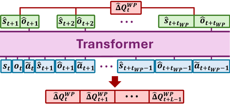
Figure 3: Planning with Transformer

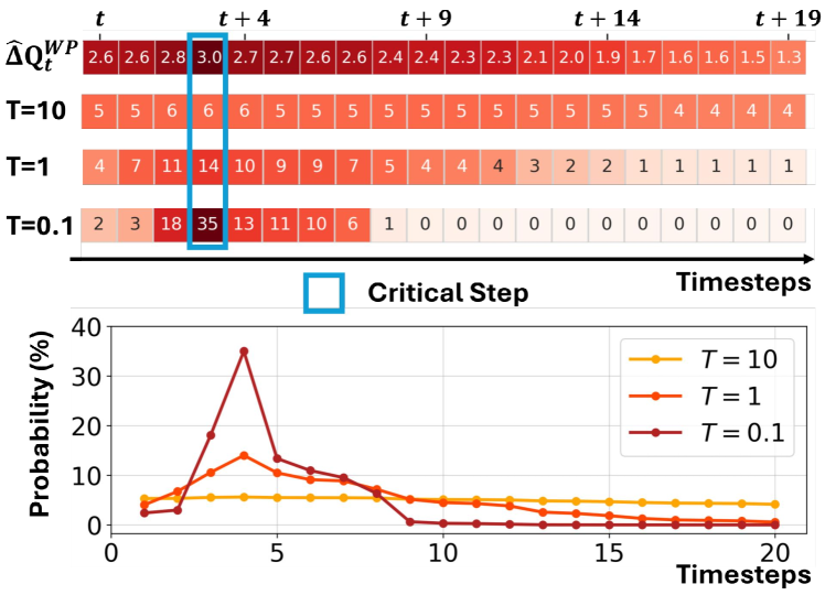
Figure 4: Attacking step probabilites

For planning, we employ a Transformer (Vaswani, 2017), commonly used in sequential learning, which leverages an attention mechanism for efficient learning. As shown in Fig. 3, the Transformer learns environment dynamics $P$ using replay buffer trajectories to predict future states and observations $(\hat{s}_{t+1},\hat{\mathbf{o}}_{t+1},\cdots,\hat{s}_{t+t_{\mathrm{WP}}},\hat{\mathbf{o}}_{t+t_{\mathrm{WP}}})$, where $\mathbf{o}_{t}$ represents the joint observation used to compute $Q^{tot}$. Actions $\tilde{\mathbf{a}}_{l}=\pi_{\mathrm{adv}}^{\mathrm{WP}}(\hat{s}_{l},\mathbf{a}_{l},k_{l})$ for $\mathbf{a}_{l}\sim\pi$ are generated by $\pi_{\mathrm{adv}}^{\mathrm{WP}}$ for $l=t,\cdots,t+t_{\mathrm{WP}}$, with $\hat{s}_{t}=s_{t}$. Using the planner, we estimate the $Q$-value reduction $\hat{\Delta}Q_{t}^{\mathrm{WP}}$ caused by the Wolfpack attack. For $L$ time steps $l=t,\cdots,t+L-1$, we compute future $Q$-differences $\hat{\Delta}Q_{l}^{\mathrm{WP}}$ and select $t_{\mathrm{init}}$ based on the initial attack probability $P_{t,\mathrm{attack}}$:

$$P_{t,\mathrm{attack}}=\left\{\mathrm{Soft}\left(\hat{\Delta}Q_{t}^{\mathrm{WP}}/T,\cdots,\hat{\Delta}Q_{t+L-1}^{\mathrm{WP}}/T\right)\right\}_{1},$$ (3)

where ${\mathbf{x}}_{l}$ indicates the $l$-th element of $\mathbf{x}$, and $T>0$ is the temperature. In this paper, we set $L=20$ as it provides an appropriate attack period. After selecting $K_{\mathrm{WP}}$ initial attacks, no further attacks are performed. Fig. 4 shows how step probabilities are distributed for different $T$ values ($T=0.1,1,10$). At each time $t$, the planner predicts $\hat{\Delta}Q_{t}^{\mathrm{WP}}$ for $t$ to $t+L-1$, forming soft initial attack probabilities. A larger $T$ results in more uniform probabilities, while a smaller $T$ increases the likelihood of targeting critical steps where $\hat{\Delta}Q_{t}^{\mathrm{WP}}$ is highest. These critical steps are selected with the highest probabilities for initial attacks. In Section 5, we analyze the effectiveness of this method in delivering more critical attacks compared to Random Step Selection and examine the impact of $T$ on performance in practical environments. Since the proposed method involves planning at every evaluation, we also train a separate model to predict $\hat{\Delta}Q_{t}^{\mathrm{WP}}$, significantly reducing computational complexity. Details of this approach and the Transformer training loss functions are provided in Appendix B.1.

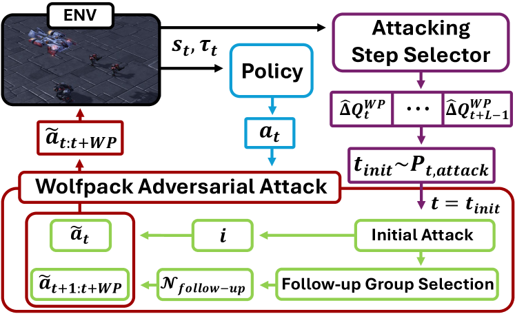
Figure 5: Illustration of the proposed WALL framework

4.5 WALL: A Robust MARL Algorithm

Similar to other robust MARL methods, we propose the Wolfpack-Adversarial Learning for MARL (WALL) framework, a robust policy designed to counter the Wolfpack attack by performing MARL on the LPA-Dec-POMDP $\tilde{\mathcal{M}}$ with the Wolfpack attacker $\pi_{\mathrm{adv}}^{\mathrm{WP}}$. We utilize well-known CTDE algorithms, including VDN (Sunehag et al., 2017), QMIX (Rashid et al., 2020), and QPLEX (Wang et al., 2020b). Detailed implementations, including loss functions for the planner transformer and the value functions, are provided in Appendix B.2. The proposed WALL framework is illustrated in Fig. 5 and summarized in Algorithm 1.

Algorithm 1 WALL framework

1: Initialize: Value function $Q^{tot}$, Planning Transformer

2: for each training iteration do

3:  for each environment step $t$ do

4:   Sample the action $\mathbf{a}_{t}$: $a_{t}^{i}\sim\epsilon$-greedy($Q^{i}$)

5:   Compute $P_{t,\mathrm{attack}}$ using Planner and sample $t_{\mathrm{init}}$

6:   if $t=t_{\mathrm{init}}$ then

7:    Perform the initial attack: $\tilde{\mathbf{a}}_{t}\sim\pi_{\mathrm{adv}}^{\mathrm{WP}}$

8:   else if $t_{\mathrm{init}}+1\leq t\leq t_{\mathrm{init}}+t_{\mathrm{WP}}$ then

9:    Select the follow-up agent group $\mathcal{N}_{\mathrm{follow-up}}$

10:    Perform the follow-up attack: $\tilde{\mathbf{a}}_{t}\sim\pi_{\mathrm{adv}}^{\mathrm{WP}}$

11:   else

12:    Execute the original action $\mathbf{a}_{t}$

13:   end if

14:  end for

15:  Update the $Q^{tot}$ using a CTDE algorithm

16:  Update the Planning Transformer

17: end for

5 Experiments

In this section, we evaluate the proposed methods in the Starcraft II Multi-Agent Challenge (SMAC) (Samvelyan et al., 2019) environment, a benchmark in MARL research. Specifically, we compare: (1) the impact of the proposed Wolfpack adversarial attack against other adversarial attacks, and (2) the robustness of the WALL framework in defending against such attacks compared to other robust MARL methods. Also, an ablation study analyzes the effect of the proposed components and hyperparameters on robustness. All results are reported as the mean and standard deviation (shaded areas for graphs and $\pm$ values for tables) across 5 random seeds.

		2s3z $K_{\mathrm{WP}}=2$ $t_{\mathrm{WP}}=3$	3m $K_{\mathrm{WP}}=1$ $t_{\mathrm{WP}}=3$	3s_vs_3z $K_{\mathrm{WP}}=2$ $t_{\mathrm{WP}}=3$	8m $K_{\mathrm{WP}}=1$ $t_{\mathrm{WP}}=3$	MMM $K_{\mathrm{WP}}=2$ $t_{\mathrm{WP}}=3$	1c3s5z $K_{\mathrm{WP}}=2$ $t_{\mathrm{WP}}=3$	Mean
Natural	Vanilla QMIX	$98.0\pm 1.52$	$99.2\pm 1.03$	$99.2\pm 1.62$	$97.6\pm 2.10$	$99.2\pm 0.54$	$99.1\pm 1.16$	$98.7\pm 0.56$
	RANDOM	$\mathbf{99.7\pm 0.56}$	$99.1\pm 1.26$	$99.0\pm 0.88$	$99.2\pm 1.03$	$\mathbf{99.6\pm 0.62}$	$99.3\pm 1.06$	$99.3\pm 0.21$
	RARL	$97.8\pm 2.09$	$93.8\pm 3.29$	$93.1\pm 17.4$	$95.5\pm 3.75$	$90.6\pm 20.8$	$84.0\pm 33.7$	$92.5\pm 5.39$
	RAP	$98.8\pm 1.37$	$95.8\pm 4.45$	$99.5\pm 1.08$	$94.7\pm 6.79$	$95.5\pm 12.1$	$84.2\pm 16.9$	$94.7\pm 2.62$
	ERNIE	$98.2\pm 1.36$	$99.2\pm 1.24$	$99.8\pm 0.44$	$\mathbf{99.8\pm 0.54}$	$98.5\pm 1.78$	$99.2\pm 1.05$	$99.1\pm 0.59$
	ROMANCE	$96.4\pm 2.97$	$93.6\pm 13.7$	$99.7\pm 0.59$	$99.6\pm 0.62$	$96.4\pm 6.62$	$96.5\pm 4.38$	$97.0\pm 2.11$
	WALL (ours)	$99.4\pm 0.65$	$\mathbf{99.7\pm 0.82}$	$\mathbf{99.8\pm 0.67}$	$99.3\pm 0.59$	$99.0\pm 2.12$	$\mathbf{99.5\pm 0.62}$	$\mathbf{99.4\pm 0.53}$
Random Attack	Vanilla QMIX	$80.4\pm 3.24$	$69.6\pm 10.4$	$91.4\pm 4.61$	$69.0\pm 7.19$	$66.4\pm 20.5$	$94.8\pm 3.45$	$78.6\pm 2.22$
	RANDOM	$90.8\pm 3.87$	$76.4\pm 17.3$	$97.4\pm 0.68$	$80.2\pm 4.92$	$95.4\pm 5.31$	$96.0\pm 2.91$	$89.4\pm 2.54$
	RARL	$86.8\pm 4.06$	$58.7\pm 15.4$	$89.2\pm 20.4$	$70.2\pm 5.83$	$84.2\pm 5.41$	$79.1\pm 22.2$	$78.0\pm 7.26$
	RAP	$91.0\pm 4.73$	$69.2\pm 11.1$	$97.8\pm 1.62$	$85.0\pm 11.4$	$86.7\pm 30.3$	$86.6\pm 12.5$	$86\pm 3.74$
	ERNIE	$83.2\pm 6.94$	$65.2\pm 4.92$	$90.2\pm 9.23$	$76.2\pm 11.8$	$86.0\pm 18.2$	$95.6\pm 3.24$	$82.7\pm 5.27$
	ROMANCE	$90.2\pm 2.39$	$71.6\pm 10.88$	$99.6\pm 0.68$	$84.8\pm 5.00$	$86.8\pm 16.3$	$94.0\pm 1.96$	$87.8\pm 2.44$
	WALL (ours)	$\mathbf{94.6\pm 4.53}$	$\mathbf{87.4\pm 1.88}$	$\mathbf{99.8\pm 0.56}$	$\mathbf{95.8\pm 3.45}$	$\mathbf{99.4\pm 1.11}$	$\mathbf{98.6\pm 1.67}$	$\mathbf{95.9\pm 0.54}$
EGA	Vanilla QMIX	$54.0\pm 7.60$	$66.5\pm 15.5$	$72.4\pm 15.1$	$71.2\pm 20.0$	$70.6\pm 14.8$	$83.0\pm 2.61$	$69.6\pm 3.84$
	RANDOM	$65.3\pm 3.31$	$70.6\pm 38.6$	$68.8\pm 23.5$	$87.5\pm 5.53$	$84.4\pm 3.12$	$84.5\pm 2.97$	$76.9\pm 5.44$
	RARL	$62.6\pm 9.40$	$74.4\pm 12.4$	$88.4\pm 17.7$	$78.4\pm 9.16$	$83.4\pm 11.9$	$80.1\pm 11.4$	$77.9\pm 9.21$
	RAP	$70.4\pm 13.0$	$84.4\pm 7.37$	$83.8\pm 15.8$	$86.2\pm 3.81$	$83.9\pm 16.4$	$80.2\pm 5.41$	$81.5\pm 4.38$
	ERNIE	$52.4\pm 9.68$	$60.4\pm 20.1$	$83.2\pm 9.75$	$81.6\pm 8.54$	$85.0\pm 4.65$	$93.6\pm 2.26$	$76.0\pm 3.00$
	ROMANCE	$79.8\pm 2.83$	$85.8\pm 4.60$	$91.0\pm 5.19$	$90.9\pm 4.09$	$87.8\pm 11.7$	$89.6\pm 2.99$	$87.5\pm 1.69$
	WALL (ours)	$\mathbf{88.6\pm 5.43}$	$\mathbf{87.0\pm 5.45}$	$\mathbf{98.7\pm 0.84}$	$\mathbf{95.8\pm 2.96}$	$\mathbf{94.2\pm 3.85}$	$\mathbf{97.0\pm 1.32}$	$\mathbf{93.6\pm 1.58}$
Wolfpack Adversarial Attack (ours)	Vanilla QMIX	$39.8\pm 7.52$	$31.0\pm 11.8$	$84.4\pm 4.78$	$11.4\pm 13.3$	$10.4\pm 14.3$	$59.2\pm 4.25$	$39.4\pm 4.57$
	RANDOM	$60.4\pm 27.4$	$57.4\pm 30.5$	$91.0\pm 3.17$	$40.4\pm 14.8$	$63.6\pm 28.7$	$68.4\pm 19.6$	$63.5\pm 3.14$
	RARL	$52.4\pm 15.8$	$31.1\pm 20.3$	$90.0\pm 17.4$	$14.2\pm 9.71$	$51.1\pm 36.8$	$75.9\pm 13.6$	$52.5\pm 8.02$
	RAP	$60.0\pm 10.3$	$37.5\pm 10.4$	$95.4\pm 3.98$	$35.6\pm 14.4$	$47.0\pm 36.9$	$75.7\pm 26.1$	$58.5\pm 5.79$
	ERNIE	$43.2\pm 13.0$	$35.4\pm 6.25$	$94.8\pm 4.42$	$26.4\pm 10.4$	$26.2\pm 17.3$	$77.0\pm 9.33$	$50.5\pm 6.62$
	ROMANCE	$62.4\pm 5.16$	$34.8\pm 14.3$	$98.6\pm 0.68$	$28.6\pm 14.2$	$48.8\pm 17.9$	$81.2\pm 4.51$	$59.1\pm 2.08$
	WALL (ours)	$\mathbf{92.2\pm 3.77}$	$\mathbf{90.8\pm 4.92}$	$\mathbf{99.8\pm 0.56}$	$\mathbf{83.6\pm 5.01}$	$\mathbf{95.0\pm 4.56}$	$\mathbf{98.8\pm 1.62}$	$\mathbf{93.4\pm 1.18}$

Table 1: Average test win rates of robust MARL policies under various attack settings

5.1 Environmental Setup

The SMAC environment serves as a challenging benchmark requiring effective agent cooperation to defeat opponents. We evaluate the proposed method across six scenarios: 2s3z, 3m, 3s_vs_3z, 8m, MMM, and 1c3s5z. We perform parameter searches for the number of follow-up agents $m$, total Wolfpack attacks $K_{\mathrm{WP}}$, and attack duration $t_{\mathrm{WP}}$, using optimal settings for comparisons. To ensure realistic constraints, we set $m$ to $m<\left\lfloor\frac{n-1}{2}\right\rfloor$, where $n$ is the maximum number of allied units. We provide details on environment setups and experimental configurations, including hyperparameter settings, in Appendices A and C. All MARL methods are evaluated on the QMIX baseline, with comparison for other CTDE baselines in Appendix E.1.

Adversarial Attacker Baselines: To compare the severity of different attacks, we consider the following 4 scenarios: Natural, representing the case where no attacks are performed; Random Attack, where time steps, agents, and actions are randomly selected to execute attacks; Evolutionary Generation of Attackers (EGA) (Yuan et al., 2023), which combines multiple single-agent-targeted attackers generated from various seeds as described in Section 3; and the proposed Wolfpack Adversarial Attack. For a fair comparison, adversarial attackers are trained on independent seeds to execute unseen attacks.

Robust MARL Baselines: To compare the severity of attack baselines and the robustness of policies trained under adversarial attack scenarios, we evaluate QMIX-trained policies under the following attack conditions: Vanilla QMIX, assuming no adversarial attacks; RANDOM, using Random Attack; RARL (Pinto et al., 2017), where adversarial attackers tailor attacks to the learned policy; RAP (Vinitsky et al., 2020), an extension of RARL that uniformly samples attackers to prevent overfitting and introduce diversity; ROMANCE (Yuan et al., 2023), an RAP extension countering diverse EGA attacks; ERNIE (Bukharin et al., 2024), enhancing robustness via adversarial regularization in observations and actions; and the proposed WALL.

All robust MARL methods follow author-provided methodologies and parameters. Further details on the MARL baselines are available in Appendix D. All policies are trained for 3M timesteps, starting from a pretrained Vanilla QMIX model trained for 1M timesteps.

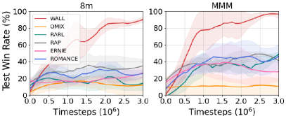
Figure 6: Learning curves of MARL methods for Wolfpack attack

5.2 Performance Comparison

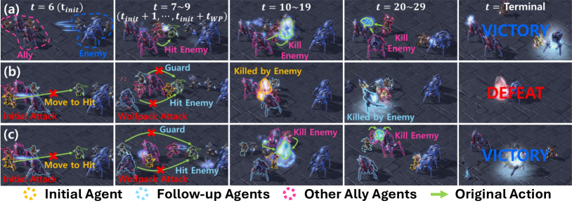
Figure 7: Attack comparison on 2s3z task in the SMAC: (a) QMIX/Natural, (b) QMIX/Wolfpack attack, and (c) WALL/Wolfpack attack

Table 1 presents the average win rates over the last 100 episodes of MARL policies against attacker baselines. The results show that the proposed Wolfpack adversarial attack is significantly more powerful than existing methods like EGA and Random Attack. For example, EGA reduces Vanilla QMIX performance by $98.7-69.6=29.1\%$ and RANDOM by $99.3-76.9=22.4\%$ compared to the Natural scenario. In contrast, the Wolfpack attack reduces Vanilla QMIX performance by $98.7-39.4=59.3\%$ and RANDOM by $99.3-63.5=35.8\%$, demonstrating its greater impact. In addition, the proposed WALL framework, trained to defend against the Wolfpack attack, outperforms other robust MARL methods against all attack types, showcasing its superior robustness. Notably, despite RANDOM is trained against Random Attack and ROMANCE against EGA, WALL achieves better performance against both attack types. This result highlights the effectiveness of WALL in enabling robust learning under diverse attack scenarios. Fig. 6 further illustrates this in the 8m and MMM environments, where performance differences with existing methods are most pronounced, showing the average win rate of each policy over training steps under unseen Wolfpack adversarial attacks. The results reveal that WALL not only achieves higher robustness but also adapts more quickly to attacks. Similar trends are observed for other CTDE algorithms, such as VDN and QPLEX, as detailed in Appendix E.1, confirming the robustness of the proposed method.

5.3 Visualization of Wolfpack Adversarial Attack

To analyze the superior performance of the Wolfpack attack, we provide a visualization of its execution in the SMAC environment. Fig. 7 illustrates a scenario where the proposed step selector identifies $t=6$ as a critical initial step to initiate the attack. Prior to $t=6$, all setups are assumed to follow the same trajectory. Fig. 7(a) shows Vanilla QMIX in a Natural scenario without attack, where our agents successfully defeat all enemy agents, achieving victory. Fig. 7(b) demonstrates Vanilla QMIX under the Wolfpack adversarial attack, with follow-up agents targeted during $t=7$ to $t=9$. This leaves other agents unable to effectively defend against the adversarial attack, resulting in defeat as all agents are killed by the enemy. Fig. 7(c) highlights a policy trained with the WALL framework. Despite the same follow-up agents are targeted during $t=7$ to $t=9$, WALL trains non-attacked agents to back up and protect the attacked agents, enabling ally agents to eliminate enemy agents and secure victory. This visualization demonstrates how the Wolfpack attack disrupts agent coordination and how the WALL framework robustly defends against such attacks. Visualizations of other SMAC tasks and detailed follow-up agent selection are provided in Appendix G.

5.4 Ablation Study

To evaluate the impact of each component and hyperparameter in the proposed Wolfpack adversarial attack, we conduct an ablation study focusing on the following aspects: component evaluation, step selection temperature $T$, and the number of follow-up agents $m$. The ablation study is conducted in the 8m and MMM environments, where the performance differences are most pronounced. Additionally, more ablation studies on other hyperparameters, such as the total number of Wolfpack attacks $K_{\mathrm{WP}}$ and the attack duration $t_{\mathrm{WP}}$, are provided in Appendix F.

Component Evaluation: To evaluate the impact of each proposed component on attack severity and policy robustness, we consider five setups: ‘Default’, which uses all proposed components as designed; ‘Init. agent (min)’, where the initial target agent $i$ is selected to minimize $Q^{tot}$, i.e., $i=\arg\min_{j}{\min_{a^{j}}Q^{tot}(s_{t_{\mathrm{init}}},a_{t_{\mathrm{init}}}^{j},\mathbf{a}_{t{\mathrm{init}}}^{-j})},$ instead of random selection; ‘Follow-up (L2)’, which selects $m$ agents closest to the initial agent based on L2 distance instead of the proposed follow-up selection method; ‘Step (Random)’, which uses random step selection instead of the proposed step selection method, while keeping the same total number of attacks; and ‘Agents & Step (Random)’, which randomly selects both $m$ follow-up agents and attack steps.

For each setup, we train the Wolfpack adversarial attack and the corresponding robust policy of WALL. Fig. 8(a) shows the robustness of WALL trained under each setup when exposed to the default Wolfpack attack, while Fig. 8(b) illustrates how each attack setup degrades the performance of ‘Vanilla QMIX’ compared to its ‘Natural’ performance. Randomly selecting the initial agent yields more robust policies than selecting the agent minimizing $Q^{tot}$ (‘Init. agent (min)’), as random selection introduces diversity in attack scenarios. While selecting the $Q^{tot}$-minimizing agent may slightly enhance attack severity in cases like MMM, the added diversity from random selection generally improves robustness. Comparing ‘Default’ and ‘Follow-up (L2)’ shows that the proposed follow-up selection method enables more severe attacks and trains more robust policies than simply targeting agents closest to the initial agent. Similarly, ‘Default’ outperforms ‘Step (Random)’ in both attack severity and robustness, demonstrating that the proposed planner effectively identifies critical steps to minimize $Q^{tot}$, producing stronger policies. Finally, ‘Default’ achieves significantly better robustness and more critical attacks compared to ‘Agents & Step (Random)’, highlighting the combined effectiveness of the proposed components.

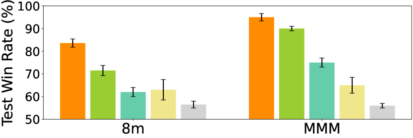
(a) Robustness of WALL variations

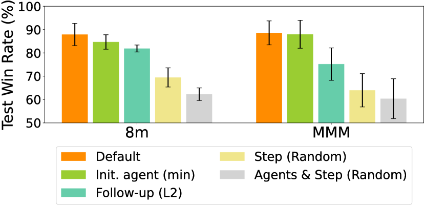
(b) Degradation of Vanilla QMIX under each attack setup

Figure 8: Component Evaluation of WALL and Wolfpack attack

Number of Follow-up Agents $m$: To analyze the impact of the hyperparameter $m$, which determines the number of follow-up agents, on robustness, Fig. 9 shows how WALL trained with different values of $m$ defend against the default Wolfpack attack. To prevent excessive attack that could cause learning to fail, we assume $m<\left\lfloor\frac{n-1}{2}\right\rfloor$. The results indicate that in the 8m environment, when $m$ is small, only a few agents defending against the initial attack are targeted, leading to reduced robustness. Conversely, when $m=4$, too many agents are attacked, causing learning to deteriorate. Therefore, $m=3$ yields the most robust performance and is considered the default hyperparameter. Similarly, in the MMM environment, $m=4$ results in the most robust performance and is set as the default. Notably, when $m=1$, the attack becomes a single-agent attack. As discussed in Section 4.1, performing coordinated multi-agent attack ($m>1$) enables much more robust learning, demonstrating the effectiveness and superiority of the proposed Wolfpack attack framework.

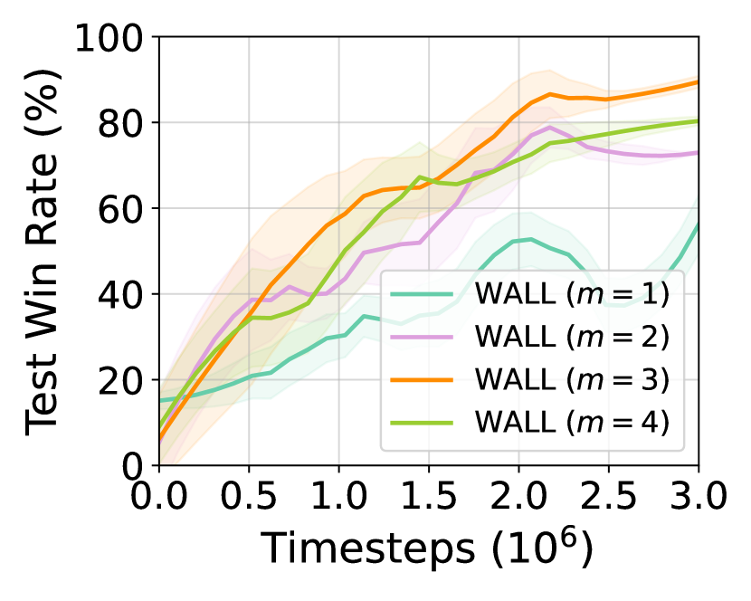
(a) 8m

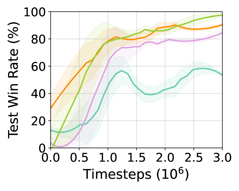
(b) MMM

Figure 9: Number of Follow-up Agents ($m$)

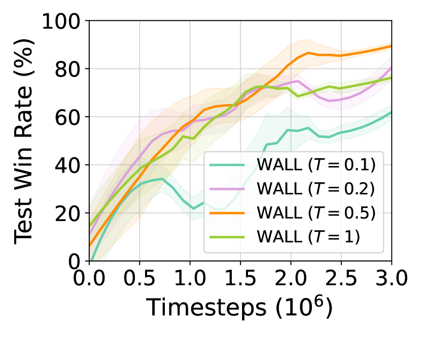
(a) 8m

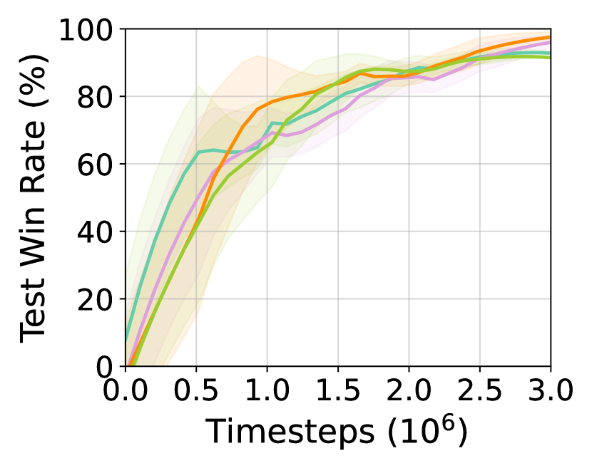
(b) MMM

Figure 10: Step Selection Temperature ($T$)

Step Selection Temperature $T$: $T$ is a hyperparameter in Eq. (3) that controls the temperature of the initial attack probability. A larger $T$ results in more random attacks across steps, while a smaller $T$ focuses attacks on critical steps with higher probability. Fig. 10 illustrates the performance of WALL policies trained with varying values of $T$ against the default Wolfpack attack. In both the 8m and MMM environments, a very small $T$ causes the attack to target only specific steps, leading to policies that are less robust against diverse attacks. Conversely, a very large $T$ leads to overly uniform attacks, failing to target critical steps effectively, which also results in less robust policies. Based on these findings, we determined that $T=0.5$ strikes a balance between targeting critical steps and maintaining robustness, and we set this as the default parameter.

6 Conclusions

In this paper, we propose the Wolfpack adversarial attack, a coordinated strategy inspired by the Wolfpack tactic used in military operations, which significantly outperforms existing adversarial attacks. Additionally, we develop WALL, a robust MARL method designed to counter the proposed attack, demonstrating superior performance across various SMAC environments. Overall, our WALL framework enhances the robustness of MARL algorithms.

Impact Statement

This paper presents work whose goal is to advance the field of Machine Learning. There are many potential societal consequences of our work, none which we feel must be specifically highlighted here.

Appendix A Environmental Setup

All experiments in this paper are conducted in the SMAC (Samvelyan et al., 2019) environment, and this section provides a detailed description of its setup and features.

SMAC
The StarCraft Multi-Agent Challenge (SMAC) serves as a benchmark for cooperative Multi-Agent Reinforcement Learning (MARL), focusing on decentralized micromanagement tasks. Based on the real-time strategy game StarCraft II, SMAC requires each unit to be controlled by independent agents acting solely on local observations. It offers a variety of combat scenarios to evaluate MARL methods effectively.

Scenarios
SMAC scenarios involve combat situations between an allied team controlled by learning agents and an enemy team managed by a scripted AI. These scenarios vary in complexity, unit composition, and terrain, challenging agents to use advanced micromanagement techniques such as focus fire, kiting, and terrain exploitation. Scenarios end when all units on one side are eliminated or when the time limit is reached. The objective is to maximize the win rate of the allied agents. Detailed descriptions of the scenarios and unit compositions are provided in Table A.1 and Figure A.1.

States and observations
In the SMAC environment, each agent receives partial observations, which contain information about visible allies and enemies within a fixed sight range of 9 units. These observations do not include global state information and are limited to the agent’s local view of the environment. Observations are specifically designed to support decentralized decision-making by individual agents, without access to global state features.

The global state, used during centralized training, aggregates the features of all agents and enemies. The state dimensionality depends on:

• Ally state: A variable size based on the number of agents ($n_{\text{agents}}$), including their relative x (dim = $1$), relative y (dim = $1$), health (dim = $1$), energy (dim = $1$), shield (dim = $\mathrm{shield\_dim}$), and unit type (dim = $\mathrm{unit\_type\_dim}$). For each ally, the total feature size is $n_{\text{agents}}\times(4+\mathrm{shield\_dim}+\mathrm{unit\_type\_dim})$.

• Enemy state: Similar to Ally state but excludes energy. For each enemy, the total feature size is $n_{\text{enemies}}\times(3+\mathrm{shield\_dim}+\mathrm{unit\_type\_dim})$.

• Last action: Represents the most recent action taken by each agent. The total feature size is $n_{\text{agents}}\times n_{\text{actions}}$. Here, $n_{\text{actions}}$ refers to the number of actions.

These features are concatenated to form the observation vector for each agent. The dimensionality of the observation vector depends on the following factors:

• Movement features: A fixed size representing available movement directions (dim = $4$).

• Enemy features: A variable size based on the number of enemies ($n_{\text{enemies}}$), including their available action (dim = $1$), distance (dim = $1$), relative x (dim = $1$), relative y (dim = $1$), health (dim = $1$), shield (dim = $\mathrm{shield\_dim}$, where $\mathrm{shield\_dim}=1$ for Protoss units and $0$ otherwise), and unit type (dim = $\mathrm{unit\_type\_dim}$, where $\mathrm{unit\_type\_dim}=0$ if there is 1 agent type, otherwise equals the number of agent types). For each enemy, the total feature size is $n_{\text{enemies}}\times(5+\mathrm{shield\_dim}+\mathrm{unit\_type\_dim})$.

• Ally features: A variable size based on the number of allies ($n_{\text{allies}}$), where $n_{\text{allies}}=n_{\text{agents}}-1$, similar to Enemy features. For each ally, the total feature size is $n_{\text{allies}}\times(5+\mathrm{shield\_dim}+\mathrm{unit\_type\_dim})$.

• Own features: Includes health (dim = $1$), shield (dim = $\mathrm{shield\_dim}$), and unit type (dim = $\mathrm{unit\_type\_dim}$). The total feature size is $1+\mathrm{shield\_dim}+\mathrm{unit\_type\_dim}$.

The precise dimensions of the observation and state vectors vary across different maps, as summarized in Table A.1.

Action space
Agents can perform discrete actions, including movement in four cardinal directions (North, South, East, West), attacking specific enemy units within a shooting range of 6 units, and specialized actions such as healing for units like Medivacs. Additionally, agents can perform a stop or a no-op action, the latter being restricted to dead units.

The size of the action space varies depending on the scenario and is defined as $n_{\text{actions}}=6+n_{\text{enemies}}$, where $6$ represents movement, stop, or a no-op action. The inclusion of $n_{\text{enemies}}$ accounts for the need to specify which enemy unit is targeted when performing an attack action. The exact size of the action space varies across different maps, as summarized in Table A.1.

Rewards
SMAC uses a shaped reward function $R$ to guide learning, including components for damage dealt ($R_{\text{damage}}$), enemy units killed ($R_{\text{enemy\_killed}}$), and scenario victory ($R_{\text{win}}$). The total reward is defined as:

$$R =\sum_{e\in\text{enemies}}\Delta\text{Health}(e)+\sum_{e\in\text{enemies}}\mathbb{I}(\{\text{Health}(e)=0\})\cdot\text{Reward}_{\text{death}}+\mathbb{I}(\{\text{win}=\text{True}\})\cdot\text{Reward}_{\text{win}}$$

Here, $\text{Health}(e)$ represents the health of an enemy unit $e$, and $\Delta\text{Health}(e)$ is the reduction in its health during a timestep. The indicator function $\mathbb{I}(\cdot)$ returns $1$ if the condition inside is true and $0$ otherwise. The parameters $\text{Reward}_{\text{death}}$ and $\text{Reward}_{\text{win}}$ are scaling factors for rewards when an enemy unit is killed and when the agents win the scenario, set to $10$ and $200$, respectively.

Map	Ally Units	Enemy Units	State Dim	Obs Dim	Action Space
3m	3 Marines	3 Marines	48	30	9
3s_vs_3z	3 Stalkers	3 Zealots	54	36	9
2s3z	2 Stalkers,	2 Stalkers,	120	80	11
	3 Zealots	3 Zealots
8m	8 Marines	8 Marines	168	80	14
1c3s5z	1 Colossus,	1 Colossus,	270	162	15
	3 Stalkers,	3 Stalkers,
	5 Zealots	5 Zealots
MMM	1 Medivac,	1 Medivac,	290	160	16
	2 Marauders,	2 Marauders,
	7 Marines	7 Marines

Table A.1: SMAC Scenarios with Units and Dimensions of State, Observation, and Action Space

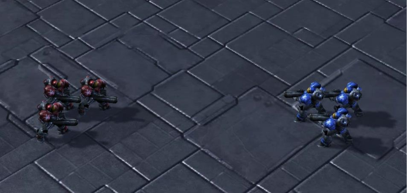
(a) 3m

(b) 3s_vs_3z

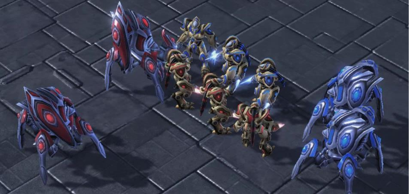
(c) 2s3z

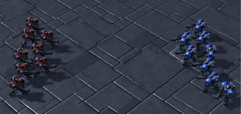
(d) 8m

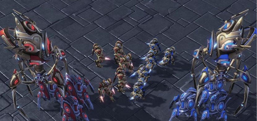
(e) 1c3s5z

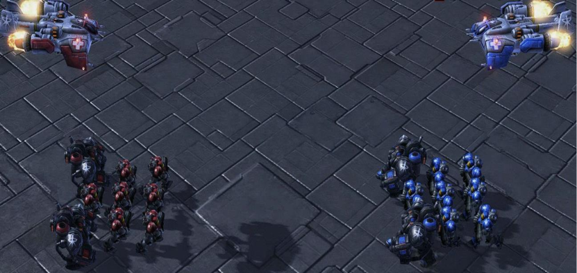
(f) MMM

Figure A.1: Visualization of SMAC Scenarios

Appendix B Implementation Details

In this section, we provide a detailed implementation of the proposed WALL framework. Section B.1 outlines the implementation of the transformer used to efficiently identify critical initial steps. Section B.2 elaborates on the components constituting the Wolfpack attack and provides an in-depth explanation of the reinforcement learning implementation.

B.1 Practical Implementation of Planner Transformer

Critical attacking step selection introduced in Section 4.4 requires planning to compute the reduction in $Q$-function values, $\Delta Q_{l}^{\mathrm{WP}}$ ($l=t,\cdots,t+L-1$), over multiple time steps. To facilitate this process, a transformer model is employed. During training, the transformer predicts $(\hat{s}_{t+1},\hat{\mathbf{o}}_{t+1},\cdots,\hat{s}_{t+t_{\mathrm{WP}}},\hat{\mathbf{o}}_{t+t_{\mathrm{WP}}})$ at the current step $t$ to compute the target $\hat{\Delta}Q_{t}^{\mathrm{WP}}$. However, performing this planning process at each evaluation step to calculate the probability of an initial attack, $P_{t,\mathrm{attack}}$, is computationally expensive.

To address this, the single transformer is split into two components: a planning transformer and a $Q$-difference transformer. The planning transformer predicts $(\hat{s}_{t+1},\hat{\mathbf{o}}_{t+1})$ and is used only during training, while the $Q$-difference transformer predicts $\Delta Q_{l}^{\mathrm{WP}}$ ($l=t,\cdots,t+L-1$) and is employed exclusively during evaluation. This separation enables efficient computation of $P_{t,\mathrm{attack}}$ during evaluation, significantly reducing computational costs. Both transformers adopt the Decision Transformer structure (Chen et al., 2021), consisting of transformer decoder layers. The planning transformer is parameterized by $\phi_{\mathrm{planning}}$, and the $Q$-difference transformer by $\phi_{\mathrm{qdiff}}$. Their respective loss functions are defined as:

$$\mathcal{L}_{\mathrm{planning}}(\phi_{\mathrm{planning}}) =\mathbb{E}\left[\|s_{t+1}-\hat{s}_{t+1}(\phi_{\mathrm{planning}})\|^{2}+\|\mathbf{o}_{t+1}-\hat{\mathbf{o}}_{t+1}(\phi_{\mathrm{planning}})\|^{2}\right],$$ (B.1)

$$\mathcal{L}_{\mathrm{qdiff}}(\phi_{\mathrm{qdiff}}) =\mathbb{E}\left[\|\Delta Q_{t}^{\mathrm{WP}}-\hat{\Delta}Q_{t}^{\mathrm{WP}}(\phi_{\mathrm{qdiff}})\|^{2}\right],~\forall t.$$ (B.2)

As shown in Fig. B.1, the estimated state $\hat{s}_{t+1}$ and observations $\hat{\mathbf{o}}_{t+1}$ are generated by the planning Transformer, which takes previous trajectories as input. Similarly, the estimated $Q$-difference $\hat{\Delta}Q_{t}^{\mathrm{WP}}$ is produced by the $Q$-diff Transformer, using previous states as input. The loss function $\mathcal{L}_{\mathrm{planning}}$ minimizes the prediction error for the next state $s{t+1}$ and observation $\mathbf{o}{t+1}$, while $\mathcal{L}_{\mathrm{qdiff}}$ minimizes the prediction error for $\Delta Q_{l}^{\mathrm{WP}}$ resulting from the Wolfpack attack. Figure B.1 illustrates the architectures of the transformers, where (a) represents the planning Transformer and (b) represents the $Q$-diff Transformer.

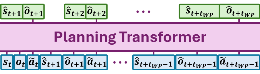
(a) Planning Transformer

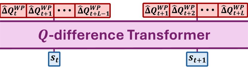
(b) $Q$-difference Transformer

Figure B.1: Structure of Transformers

B.2 Detailed Implementation of WALL

The WALL framework trains robust MARL policies to counter the Wolfpack adversarial attack by employing a $Q$-learning approach within the CTDE paradigm. Each agent computes its individual $Q$-values, $Q^{i}(\tau_{t}^{i},a_{t}^{i}),~i=1,\cdots,n$, using separate $Q$-networks. These individual values, along with the global state, are combined through a mixing network to produce the total $Q$-value, $Q_{\theta}^{tot}$, parameterized by $\theta$. This joint value function ensures effective coordination among agents under adversarial scenarios.

To achieve robustness, the training process minimizes the temporal difference (TD) loss, which incorporates the observed rewards, state transitions, and target $Q$-values parameterized by a separate target network, $\theta^{-}$. By leveraging this target network, the CTDE frameworks stabilize learning and mitigates the impact of the Wolfpack attack. The TD loss is defined as:

$$\mathcal{L}_{\text{TD}}(\theta)=\mathbb{E}_{s,\mathbf{a},r,s^{\prime}}\left[\left(r_{t}+\gamma\max_{\mathbf{a}^{\prime}}Q_{\theta^{-}}^{tot}(s_{t+1},\mathbf{a}^{\prime})-Q_{\theta}^{tot}(s_{t},\mathbf{a}_{t})\right)^{2}\right],$$ (B.3)

where the target network parameter $\theta^{-}$ is updated by applying the exponential moving average (EMA) to $\theta$. This training mechanism allows agents to adapt and develop robust policies capable of resisting the coordinated disruptions caused by the Wolfpack adversarial attack, ensuring enhanced performance and resilience in MARL scenarios. In addition, we use 3 value-based CTDE algorithms as baselines for the WALL framework: QMIX, VDN, and QPLEX. Below, we provide an outline of the key details of these baseline algorithms:

Value-Decomposition Networks (VDN)
VDN (Sunehag et al., 2017) is a $Q$-learning algorithm designed for cooperative MARL. It introduces an additive decomposition of the joint $Q$-value into individual agent $Q$-values, enabling centralized training and decentralized execution. The joint action-value function, $Q^{tot}$, is expressed as:

$$Q^{tot}(s_{t},\mathbf{a}_{t})=\sum_{i=1}^{n}Q^{i}(\tau_{t}^{i},a_{t}^{i}),$$ (B.4)

allowing agents to act independently during execution by relying only on their local $Q^{i}$ values.

QMIX
QMIX (Rashid et al., 2020) extends VDN by introducing a more expressive, non-linear representation of the joint $Q$-value, while maintaining a monotonic relationship between $Q^{tot}$ and individual agent $Q$-values, $Q^{i}(\tau^{i},a^{i})$. This ensures individual-global-max (IGM) condition:

$$\frac{\partial Q^{tot}}{\partial Q^{i}}\geq 0,\forall i,$$ (B.5)

guaranteeing consistency between centralized and decentralized policies. Specifically:

$$\arg\max_{\mathbf{a}}Q^{\text{tot}}(s_{t},\mathbf{a}_{t})=\begin{pmatrix}\arg\max_{a^{1}}Q^{1}(\tau_{t}^{1},a_{t}^{1}),\\ \vdots\\ \arg\max_{a^{n}}Q^{n}(\tau_{t}^{n},a_{t}^{n})\end{pmatrix}.$$ (B.6)

QMIX combines agent networks, a mixing network, and hypernetworks, where hypernetworks dynamically parameterize the mixing network based on the global state $s_{t}$. The weights generated by the hypernetworks are constrained to be non-negative to enforce the monotonicity constraint.

QPLEX
QPLEX (Wang et al., 2020b) introduces a duplex dueling architecture to enhance the representation of joint action-value functions while adhering to the IGM principle. QPLEX reformulates the IGM principle in an advantage-based form:

$$\arg\max_{\mathbf{a}}A^{tot}(\tau,\mathbf{a})=\begin{pmatrix}\arg\max_{a^{1}}A^{1}(\tau^{1},a^{1}),\\ \vdots\\ \arg\max_{a^{n}}A^{n}(\tau^{n},a^{n})\end{pmatrix},$$ (B.7)

where $A^{tot}$ and $A^{i}$ are the advantage functions for joint and individual action-value functions, respectively. The joint action-value function is expressed as:

$$Q^{tot}(\tau,\mathbf{a})=\sum_{i=1}^{n}Q^{i}(\tau,a^{i})+\sum_{i=1}^{n}(\lambda_{i}(\tau,\mathbf{a})-1)A^{i}(\tau,a^{i}).$$ (B.8)

where $\lambda_{i}(\tau,\mathbf{a})>0$ are importance weights generated using a multi-head attention mechanism to enhance expressiveness.

Here, VDN and QMIX are implemented using the PyMARL codebase https://github.com/oxwhirl/pymarl, while QPLEX is implemented using its official codebase https://github.com/wjh720/QPLEX.

Appendix C Experimental Details

All experiments in this paper are conducted on a GPU server equipped with an NVIDIA GeForce RTX 3090 GPU and AMD EPYC 7513 32-Core processors running Ubuntu 20.04 and PyTorch. We follow the implementations and loss scales provided by the CTDE algorithms and focus on parameter searches for hyperparameters related to the proposed Wolfpack adversarial attack. Comparisons are performed using the optimal hyperparameter setup, with an ablation study available in Appendix F.

C.1 Hyperparameter Setup

We conduct parameter search for the number of Wolfpack attacks $K_{\mathrm{WP}}\in[1,2,3,4]$, the attack duration $t_{\mathrm{WP}}\in[1,2,3,4]$, the number of follow-up agents $m$, and the temperature $T\in[0.1,0.2,0.5,1.0]$. The total number of attacks $K$ is then determined based on $K=K_{\mathrm{WP}}\times(t_{\mathrm{WP}}+1)$, separated into training and testing setups. During training, $K$ is selected through hyperparameter sweeping to ensure optimal performance. For testing, $K$ is unified across all adversarial attack setups, including Random Attack, EGA, and the Wolfpack Adversarial Attack, to ensure fair comparisons. Additionally, the attack period $L$ is chosen based on the average episode length of SMAC scenarios and the total number of attacks, with $L=20$ is fixed as appropriate. Transformer hyperparameters, shared between the Planning Transformer and $Q$-difference Transformer, such as the number of heads, decoder layers, embedding dimensions, and input sequence length, are selected to balance accuracy and computational efficiency.

The $Q$-learning hyperparameters (shared across all CTDE methods) and those specific to the CTDE algorithms are detailed in Table C.1 and Table C.2, respectively. The Wolfpack adversarial attack-related hyperparameters for the WALL framework, shared across all SMAC scenarios and scenario-specific setups, are presented in Table C.3.

Hyperparameter	Value
Epsilon	1.0 $\rightarrow$ 0.05
Epsilon Anneal Time	50000 timesteps
Train Interval	1 episode
Gamma	0.99
Critic Loss	MSE Loss
Buffer Size	5000 episodes
Batch Size	32 episodes
Agent Learning Rate	0.0005
Critic Learning Rate	0.0005
Optimizer	RMSProp
Optimizer Alpha	0.99
Optimizer Eps	1e-5
Gradient Clip Norm	10.0
Num GRU Layers	1
RNN Hidden State Dim	64
Double Q	True

Table C.1: Common $Q$-learning Hyperparameters

Hyperparameter	VDN	QMIX	QPLEX
Mixer	VDN	QMIX	QPLEX
Mixing Embed Dim	-	32	32
Hypernet Layers	-	2	2
Hypernet Embed Dim	-	64	64
Adv Hypernet Layers	-	-	1
Adv Hypernet Embed Dim	-	-	64
Num Kernel	-	-	2

Table C.2: VDN, QMIX, QPLEX Hyperparameters

Common Hyperparameters	Value
Attack duration ($t_{\mathrm{WP}}$)	3
Temperature ($T$)	0.5
Attack Period ($L$)	20
Num Transformer Head	1
Num Transformer Decoder Layer	1
Transformer Embed Dim	64
Input Sequence Length	20

Scenario	3m	3s_vs_3z	2s3z	8m	1c3s5z	MMM
Num Total Attacks (Train) ($K$)	8	16	12	8	16	16
Num Total Attacks (Test) ($K$)	8	4	8	4	8	8
Num Wolfpack Attacks ($K_{\mathrm{WP}}$)	2	4	3	2	4	4
Num Follow-up Agents ($m$)	1	1	2	3	4	4

Table C.3: Wolfpack hyperparameters shared across scenarios and scenario-specific values

Appendix D Details of Other Robust MARL Methods

In this section, we detail various robust MARL methods compared against the proposed WALL framework, as below:

Robust Adversarial Reinforcement Learning (RARL)
RARL (Pinto et al., 2017) enhances policy robustness by training a protagonist agent and an adversary in a two-player zero-sum Markov game. At each timestep $t$, the agents observe state $s_{t}$ and take actions $a_{t}^{1}\sim\mu(s_{t})$ and $a_{t}^{2}\sim\nu(s_{t})$, where $\mu$ is the protagonist’s policy, and $\nu$ is the adversary’s policy. The state transitions follow:

$$s_{t+1}=P(s_{t},a_{t}^{1},a_{t}^{2}).$$ (D.9)

The protagonist maximizes its cumulative reward $R^{1}$, while the adversary minimizes it:

$$R^{1}_{*}=\min_{\nu}\max_{\mu}R^{1}(\mu,\nu)=\max_{\mu}\min_{\nu}R^{1}(\mu,\nu).$$ (D.10)

Robustness via Adversary Populations (RAP)
RAP (Vinitsky et al., 2020) improves robustness by training agents against a population of adversaries, reducing overfitting to specific attack patterns. During training, an adversary is sampled uniformly from the population ${\pi_{\phi_{1}},\pi_{\phi_{2}},\dots,\pi_{\phi_{n}}}$. The objective is:

$$\max_{\theta}\min_{\phi_{1},\dots,\phi_{n}}\mathbb{E}_{i\sim U(1,n)}\left[\sum_{t=0}^{T}\gamma^{t}r(s_{t},a_{t},\alpha a_{t}^{i})\middle|\pi_{\theta},\pi_{\phi_{i}}\right],$$ (D.11)

where $\pi_{\theta}$ is the agent’s policy, $\pi_{\phi_{i}}$ is the $i$-th adversary, and $\alpha$ controls adversary strength.

Robust Multi-Agent Coordination via Evolutionary Generation of Auxiliary Adversarial Attackers (ROMANCE)
ROMANCE (Yuan et al., 2023) generates diverse auxiliary adversarial attackers to improve robustness in CMARL. Its objective combines attack quality and diversity:

$$L_{\text{adv}}(\phi)=\frac{1}{n_{p}}\sum_{j=1}^{n_{p}}L_{\text{opt}}(\phi_{j})-\alpha L_{\text{div}}(\phi),$$ (D.12)

where $L_{\text{opt}}$ minimizes the ego-system’s return, $L_{\text{div}}$ promotes diversity using Jensen-Shannon Divergence, and $n_{p}$ is the number of adversarial policies. ROMANCE uses an evolutionary mechanism to explore diverse attacks.

We implement RARL and RAP for multi-agent systems, as well as ROMANCE with EGA, using the ROMANCE codebase available at https://github.com/zzq-bot/ROMANCE.

ERNIE
ERNIE (Bukharin et al., 2024) improves robustness by promoting Lipschitz continuity through adversarial regularization. It minimizes discrepancies between policy outputs under perturbed and non-perturbed observations:

$$R_{\pi}(o_{k};\theta_{k})=\max_{\|\delta\|\leq\epsilon}D(\pi_{\theta_{k}}(o_{k}+\delta),\pi_{\theta_{k}}(o_{k})),$$ (D.13)

where $o_{k}$ is the agent’s observation, $\delta$ is a bounded perturbation, and $D$ measures divergence (e.g., KL-divergence). ERNIE reformulates adversarial training as a Stackelberg game and extends its framework to mean-field MARL for scalability in large-agent settings. We evaluate ERNIE using its official codebase at https://github.com/abukharin3/ERNIE.

Appendix E Additional Experiments Results

E.1 Comparison Results for Other CTDE Algorithms

Our proposed Wolfpack attack is compatible with various value-based MARL algorithms. Experimental results in this section demonstrate its significant impact on robustness, not only in QMIX, as discussed in the main text, but also in VDN and QPLEX. The hyperparameters used in these experiments follow those outlined in Appendix C.1, with WALL hyperparameters remaining consistent across all algorithms, including QMIX.

VDN Results: Table E.1 shows the average win rates for various robust MARL methods with VDN against attacker baselines. Both models and attackers are trained using the VDN-based algorithm. Results indicate that the proposed Wolfpack attack is more detrimental than Random Attack or EGA for VDN. For example, while EGA reduces Vanilla VDN’s performance by $95.6\%-73.8\%=21.8\%$, the Wolfpack attack causes a larger reduction of $95.6\%-44.1\%=51.5\%$, demonstrating its severity. Additionally, the WALL framework outperforms other baselines under both Natural conditions and adversarial attacks, showcasing its robustness.

		2s3z $K_{\mathrm{WP}}=2$ $t_{\mathrm{WP}}=3$	3m $K_{\mathrm{WP}}=1$ $t_{\mathrm{WP}}=3$	3s_vs_3z $K_{\mathrm{WP}}=2$ $t_{\mathrm{WP}}=3$	8m $K_{\mathrm{WP}}=1$ $t_{\mathrm{WP}}=3$	MMM $K_{\mathrm{WP}}=2$ $t_{\mathrm{WP}}=3$	1c3s5z $K_{\mathrm{WP}}=2$ $t_{\mathrm{WP}}=3$	Mean
Natural	Vanilla VDN	$98.5\pm 1.35$	$96.0\pm 2.95$	$99.3\pm 0.50$	$97.8\pm 2.00$	$98.3\pm 0.50$	$83.5\pm 9.50$	$95.6\pm 1.65$
	RANDOM	$99.0\pm 0.10$	$\mathbf{99.8\pm 0.05}$	$99.4\pm 0.45$	$\mathbf{98.9\pm 0.05}$	$98.8\pm 1.00$	$97.6\pm 0.50$	$98.9\pm 0.36$
	RARL	$95.3\pm 0.50$	$92.5\pm 3.35$	$99.3\pm 0.45$	$96.3\pm 1.50$	$93.2\pm 1.50$	$91.8\pm 0.00$	$94.7\pm 0.55$
	RAP	$93.4\pm 1.30$	$96.8\pm 48.4$	$99.3\pm 0.45$	$98.7\pm 1.00$	$97.3\pm 0.50$	$97.3\pm 0.50$	$97.1\pm 0.37$
	ERNIE	$94.6\pm 3.85$	$99.4\pm 0.50$	$97.1\pm 0.47$	$98.4\pm 1.38$	$98.8\pm 0.82$	$96.5\pm 1.70$	$97.5\pm 0.86$
	ROMANCE	$98.2\pm 0.05$	$97.9\pm 1.05$	$99.4\pm 0.45$	$93.5\pm 5.35$	$97.9\pm 0.95$	$93.0\pm 3.10$	$96.6\pm 0.77$
	WALL (ours)	$\mathbf{99.8\pm 0.10}$	$99.4\pm 0.45$	$\mathbf{99.9\pm 0.10}$	$96.9\pm 2.00$	$\mathbf{99.4\pm 0.45}$	$\mathbf{100.0\pm 0.05}$	$\mathbf{99.2\pm 0.19}$
Random Attack	Vanilla VDN	$80.5\pm 1.50$	$65.5\pm 6.50$	$96.5\pm 0.50$	$52.5\pm 10.5$	$95.0\pm 1.00$	$76.5\pm 7.50$	$77.8\pm 1.92$
	RANDOM	$83.0\pm 1.00$	$\mathbf{94.5\pm 1.50}$	$96.0\pm 0.00$	$88.5\pm 0.50$	$95.5\pm 2.50$	$93.5\pm 1.50$	$91.8\pm 0.50$
	RARL	$81.0\pm 4.15$	$64.5\pm 8.40$	$97.3\pm 0.50$	$72.9\pm 0.05$	$76.3\pm 7.50$	$92.0\pm 0.20$	$80.7\pm 2.07$
	RAP	$89.8\pm 3.05$	$75.8\pm 37.9$	$97.7\pm 1.90$	$81.2\pm 0.50$	$95.2\pm 2.55$	$92.3\pm 0.50$	$88.7\pm 1.63$
	ERNIE	$80.2\pm 2.04$	$66.9\pm 2.84$	$93.1\pm 1.71$	$67.1\pm 4.92$	$89.1\pm 2.10$	$90.4\pm 4.54$	$81.1\pm 1.19$
	ROMANCE	$91.0\pm 5.00$	$79.0\pm 6.00$	$98.4\pm 0.40$	$54.0\pm 5.00$	$97.5\pm 0.50$	$92.0\pm 3.00$	$85.3\pm 0.62$
	WALL (ours)	$\mathbf{95.5\pm 1.50}$	$86.0\pm 6.00$	$\mathbf{99.4\pm 0.40}$	$\mathbf{90.0\pm 3.00}$	$\mathbf{98.5\pm 0.50}$	$\mathbf{98.1\pm 0.05}$	$\mathbf{94.6\pm 1.39}$
EGA	Vanilla VDN	$69.5\pm 7.50$	$54.5\pm 12.5$	$94.5\pm 1.50$	$59.5\pm 12.5$	$90.5\pm 2.50$	$74.5\pm 9.50$	$73.8\pm 1.00$
	RANDOM	$56.0\pm 6.00$	$73.0\pm 6.00$	$84.0\pm 13.0$	$84.5\pm 6.50$	$85.5\pm 1.50$	$86.5\pm 3.50$	$78.3\pm 2.42$
	RARL	$58.0\pm 1.15$	$79.0\pm 2.90$	$96.5\pm 0.70$	$76.7\pm 4.00$	$75.9\pm 8.20$	$81.3\pm 4.50$	$77.9\pm 1.86$
	RAP	$79.9\pm 3.05$	$93.0\pm 46.9$	$97.3\pm 0.45$	$85.7\pm 1.25$	$91.8\pm 3.75$	$87.2\pm 1.50$	$89.3\pm 0.21$
	ERNIE	$62.0\pm 14.9$	$62.5\pm 8.18$	$89.1\pm 6.58$	$74.7\pm 1.55$	$89.3\pm 2.51$	$82.2\pm 1.86$	$76.6\pm 3.62$
	ROMANCE	$86.5\pm 2.50$	$\mathbf{93.8\pm 3.00}$	$98.0\pm 0.00$	$76.5\pm 0.50$	$95.5\pm 2.50$	$92.0\pm 0.00$	$90.3\pm 0.58$
	WALL (ours)	$\mathbf{91.5\pm 0.50}$	$91.0\pm 2.00$	$\mathbf{99.0\pm 1.00}$	$\mathbf{90.0\pm 4.00}$	$\mathbf{97.5\pm 0.50}$	$\mathbf{95.5\pm 0.50}$	$\mathbf{94.1\pm 0.08}$
Wolfpack Adversarial Attack (ours)	Vanilla VDN	$54.0\pm 4.00$	$20.5\pm 5.50$	$91.5\pm 0.50$	$24.5\pm 12.5$	$18.5\pm 9.50$	$55.5\pm 2.50$	$44.1\pm 1.08$
	RANDOM	$47.0\pm 4.00$	$89.0\pm 1.00$	$90.0\pm 5.00$	$41.0\pm 14.0$	$18.5\pm 5.50$	$83.5\pm 0.50$	$61.5\pm 2.67$
	RARL	$59.5\pm 8.65$	$41.3\pm 16.4$	$96.8\pm 0.00$	$13.1\pm 2.00$	$24.3\pm 6.50$	$61.6\pm 11.7$	$49.4\pm 1.83$
	RAP	$64.3\pm 3.50$	$67.7\pm 33.8$	$98.9\pm 0.05$	$23.9\pm 6.05$	$53.3\pm 2.50$	$82.1\pm 5.40$	$65.0\pm 1.66$
	ERNIE	$33.1\pm 3.64$	$25.8\pm 6.48$	$93.0\pm 4.54$	$17.2\pm 9.46$	$23.5\pm 9.29$	$66.4\pm 13.5$	$43.2\pm 1.69$
	ROMANCE	$63.0\pm 10.0$	$46.5\pm 20.5$	$97.5\pm 0.50$	$19.5\pm 7.50$	$38.0\pm 5.00$	$83.0\pm 4.00$	$57.9\pm 3.08$
	WALL (ours)	$\mathbf{91.5\pm 2.50}$	$\mathbf{91.5\pm 2.50}$	$\mathbf{100.0\pm 0.00}$	$\mathbf{71.5\pm 1.50}$	$\mathbf{98.0\pm 1.00}$	$\mathbf{93.5\pm 4.50}$	$\mathbf{91.0\pm 0.83}$

Table E.1: Average test win rates of robust MARL policies under various attack settings (VDN)

QPLEX Results: Similarly, Table E.2 reports the average win rates various robust MARL methods with QPLEX against attacker baselines. Both models and attackers are trained using the QPLEX-based algorithm. Results reveal that the Wolfpack attack is also more detrimental for QPLEX compared to Random Attack and EGA. For instance, EGA reduces Vanilla QPLEX’s performance by $98.4\%-57.2\%=41.2\%$, whereas the Wolfpack attack results in a larger reduction of $98.4\%-33.1\%=65.3\%$. The WALL framework again demonstrates superior robustness, performing well against all attacks, including the Wolfpack attack.

		2s3z $K_{\mathrm{WP}}=2$ $t_{\mathrm{WP}}=3$	3m $K_{\mathrm{WP}}=1$ $t_{\mathrm{WP}}=3$	3s_vs_3z $K_{\mathrm{WP}}=2$ $t_{\mathrm{WP}}=3$	8m $K_{\mathrm{WP}}=1$ $t_{\mathrm{WP}}=3$	MMM $K_{\mathrm{WP}}=2$ $t_{\mathrm{WP}}=3$	1c3s5z $K_{\mathrm{WP}}=2$ $t_{\mathrm{WP}}=3$	Mean
Natural	Vanilla QPLEX	$97.1\pm 1.25$	$\mathbf{99.2\pm 0.45}$	$99.4\pm 0.50$	$97.4\pm 0.33$	$99.5\pm 0.47$	$97.1\pm 0.94$	$98.4\pm 0.07$
	RANDOM	$97.7\pm 2.11$	$98.7\pm 0.78$	$99.6\pm 0.09$	$99.1\pm 0.87$	$98.2\pm 1.23$	$98.5\pm 1.25$	$98.7\pm 0.54$
	RARL	$94.4\pm 4.54$	$89.7\pm 1.98$	$88.4\pm 6.80$	$97.8\pm 1.63$	$98.8\pm 0.82$	$94.6\pm 1.60$	$94.0\pm 1.35$
	RAP	$96.5\pm 1.70$	$96.6\pm 2.49$	$93.2\pm 0.90$	$99.1\pm 0.47$	$98.8\pm 0.78$	$97.8\pm 0.82$	$97.7\pm 0.39$
	ERNIE	$96.7\pm 2.54$	$98.8\pm 0.82$	$99.7\pm 0.08$	$98.8\pm 1.42$	$99.1\pm 0.50$	$98.4\pm 0.97$	$98.6\pm 0.55$
	ROMANCE	$97.1\pm 2.88$	$93.2\pm 5.88$	$98.8\pm 0.82$	$94.7\pm 3.18$	$\mathbf{99.7\pm 0.05}$	$99.0\pm 1.08$	$96.8\pm 1.19$
	WALL (ours)	$\mathbf{99.5\pm 0.52}$	$97.7\pm 2.13$	$\mathbf{99.9\pm 0.08}$	$\mathbf{99.8\pm 0.14}$	$99.0\pm 0.65$	$\mathbf{99.5\pm 0.64}$	$\mathbf{99.2\pm 0.29}$
Random Attack	Vanilla QPLEX	$75.2\pm 2.54$	$36.2\pm 6.63$	$81.9\pm 16.0$	$40.0\pm 9.83$	$65.3\pm 6.18$	$75.0\pm 2.79$	$62.3\pm 5.64$
	RANDOM	$85.9\pm 0.87$	$69.0\pm 5.77$	$96.2\pm 1.61$	$89.0\pm 7.67$	$91.2\pm 2.41$	$95.5\pm 1.19$	$87.8\pm 0.65$
	RARL	$81.2\pm 13.6$	$61.3\pm 13.9$	$74.7\pm 12.6$	$73.7\pm 21.6$	$92.0\pm 0.82$	$92.0\pm 2.94$	$79.1\pm 4.27$
	RAP	$90.8\pm 2.83$	$78.0\pm 6.98$	$92.1\pm 10.3$	$65.3\pm 4.50$	$95.0\pm 1.41$	$95.7\pm 1.89$	$85.0\pm 1.88$
	ERNIE	$82.0\pm 2.02$	$59.0\pm 8.98$	$93.0\pm 1.63$	$80.0\pm 1.41$	$91.3\pm 0.94$	$93.0\pm 0.82$	$83.1\pm 1.89$
	ROMANCE	$89.2\pm 2.05$	$64.9\pm 13.4$	$93.7\pm 2.05$	$51.6\pm 5.26$	$92.2\pm 4.12$	$95.2\pm 0.99$	$76.0\pm 2.84$
	WALL (ours)	$\mathbf{97.4\pm 0.86}$	$\mathbf{85.4\pm 2.45}$	$\mathbf{99.4\pm 0.45}$	$\mathbf{92.9\pm 3.49}$	$\mathbf{98.3\pm 1.16}$	$\mathbf{98.6\pm 1.23}$	$\mathbf{95.3\pm 0.69}$
EGA	Vanilla QPLEX	$48.1\pm 3.40$	$16.0\pm 5.11$	$72.5\pm 15.1$	$58.5\pm 16.8$	$71.0\pm 4.24$	$76.9\pm 1.46$	$57.2\pm 6.15$
	RANDOM	$60.5\pm 6.78$	$61.4\pm 14.9$	$82.0\pm 6.56$	$86.2\pm 3.39$	$85.3\pm 2.53$	$88.8\pm 2.53$	$77.4\pm 3.10$
	RARL	$63.4\pm 0.45$	$65.7\pm 6.24$	$71.0\pm 8.16$	$86.0\pm 6.53$	$89.7\pm 1.89$	$84.7\pm 2.05$	$76.7\pm 0.99$
	RAP	$78.5\pm 4.02$	$83.3\pm 0.94$	$85.4\pm 5.26$	$89.0\pm 2.16$	$92.7\pm 1.70$	$96.7\pm 0.47$	$88.0\pm 0.72$
	ERNIE	$64.4\pm 6.99$	$67.3\pm 10.3$	$51.7\pm 9.46$	$86.7\pm 4.71$	$86.0\pm 4.97$	$89.3\pm 4.50$	$74.2\pm 3.01$
	ROMANCE	$79.5\pm 6.02$	$80.3\pm 1.65$	$90.3\pm 1.25$	$80.7\pm 8.25$	$95.2\pm 2.02$	$92.5\pm 1.27$	$85.6\pm 1.04$
	WALL (ours)	$\mathbf{89.0\pm 3.77}$	$\mathbf{83.9\pm 2.88}$	$\mathbf{99.6\pm 0.57}$	$\mathbf{94.4\pm 1.23}$	$\mathbf{96.4\pm 1.18}$	$\mathbf{96.1\pm 0.70}$	$\mathbf{93.2\pm 0.70}$
Wolfpack Adversarial Attack (ours)	Vanilla QPLEX	$30.8\pm 4.32$	$11.8\pm 7.46$	$63.7\pm 24.3$	$30.7\pm 11.1$	$20.0\pm 12.5$	$41.9\pm 6.08$	$33.1\pm 7.08$
	RANDOM	$50.5\pm 2.92$	$16.8\pm 6.76$	$89.5\pm 5.70$	$45.6\pm 18.0$	$34.0\pm 14.1$	$82.5\pm 11.3$	$53.2\pm 4.91$
	RARL	$55.5\pm 2.05$	$27.3\pm 9.18$	$78.0\pm 4.32$	$46.0\pm 14.9$	$21.3\pm 14.4$	$79.7\pm 6.94$	$51.3\pm 2.81$
	RAP	$59.0\pm 4.72$	$50.3\pm 14.7$	$86.7\pm 8.23$	$33.7\pm 3.09$	$45.0\pm 6.98$	$93.7\pm 2.36$	$56.3\pm 3.24$
	ERNIE	$52.9\pm 6.28$	$49.0\pm 9.90$	$76.0\pm 9.90$	$42.7\pm 10.6$	$20.7\pm 10.4$	$78.7\pm 6.65$	$53.3\pm 3.56$
	ROMANCE	$57.3\pm 8.39$	$38.5\pm 13.9$	$89.7\pm 1.25$	$28.6\pm 1.10$	$46.2\pm 10.6$	$83.5\pm 5.53$	$50.8\pm 0.89$
	WALL (ours)	$\mathbf{88.3\pm 1.20}$	$\mathbf{87.6\pm 4.72}$	$\mathbf{99.7\pm 0.47}$	$\mathbf{84.5\pm 1.67}$	$\mathbf{96.3\pm 3.86}$	$\mathbf{99.3\pm 0.90}$	$\mathbf{92.6\pm 1.32}$

Table E.2: Average test win rates of robust MARL policies under various attack settings (QPLEX)

Learning Curves for VDN and QPLEX: We also analyze training curves and average test win rates across different CTDE algorithms. Graphs for the 8m and MMM environments illustrate the average win rates of each policy over training steps under unseen Wolfpack adversarial attacks. Fig. E.1 presents training curves for VDN, while Fig. E.2 shows results for QPLEX. These curves highlight that WALL not only achieves greater robustness but also adapts more quickly to attacks across VDN and QPLEX, further confirming its effectiveness beyond QMIX.

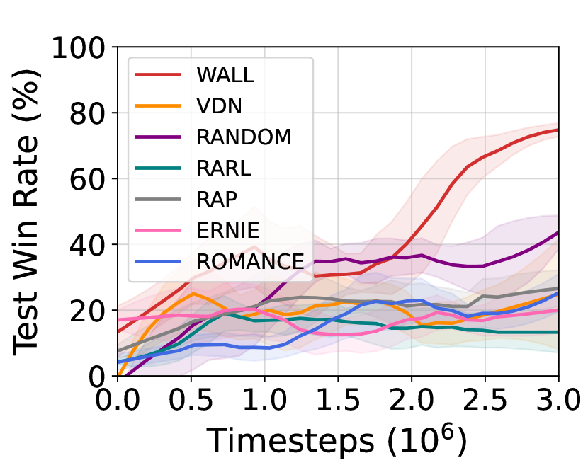
(a) 8m

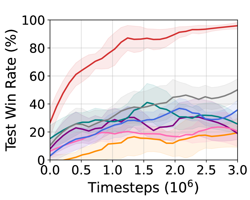
(b) MMM

Figure E.1: Learning curves of MARL methods for Wolfpack attack (VDN)

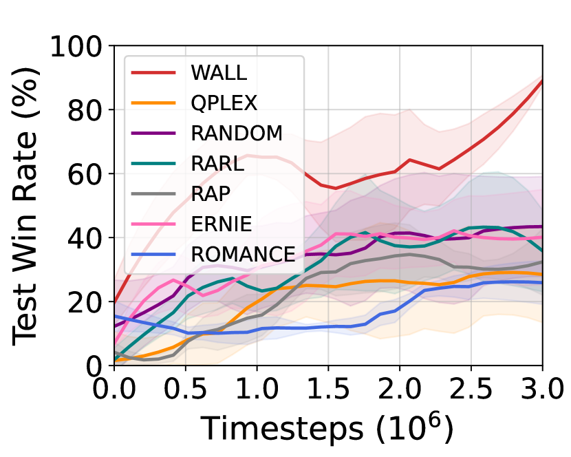
(a) 8m

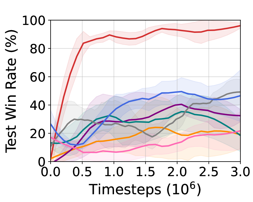
(b) MMM

Figure E.2: Learning curves of MARL methods for Wolfpack attack (QPLEX)

E.2 Learning Curves Across Additional SMAC Scenarios

In this section, we provide the training performance of WALL under Wolfpack adversarial attack across additional SMAC scenarios beyond the 8m and MMM environments, which are emphasized in the main text for their significant performance differences. Fig. E.3 illustrates the training curves for 6 scenarios: 3m, 3s_vs_3z, 2s3z, 8m, MMM, and 1c3s5z. The results demonstrate that WALL consistently outperforms baseline methods, achieving superior win rates across all scenarios. Additionally, policies trained with WALL adapt more quickly to the challenges posed by Wolfpack attack, showing robust and efficient performance across environments of varying complexity. These findings highlight the effectiveness of WALL in enhancing the robustness of MARL policies against coordinated adversarial attacks.

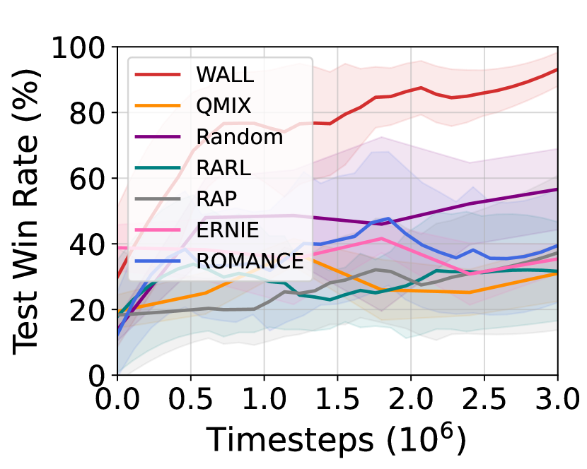
(a) 3m

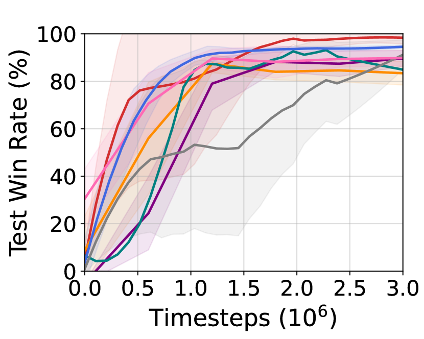
(b) 3s_vs_3z

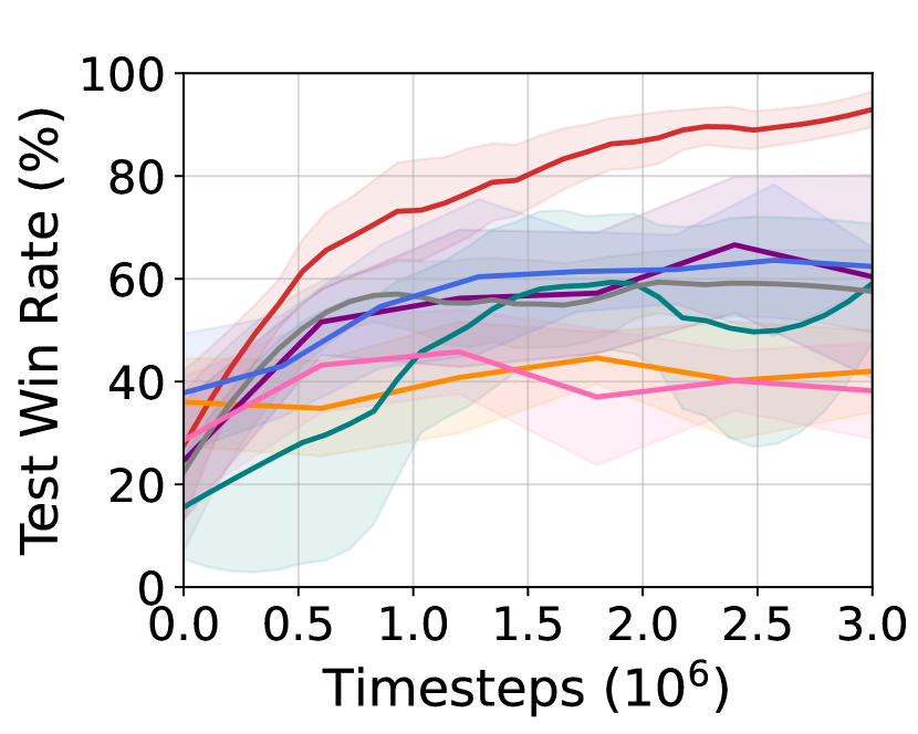
(c) 2s3z

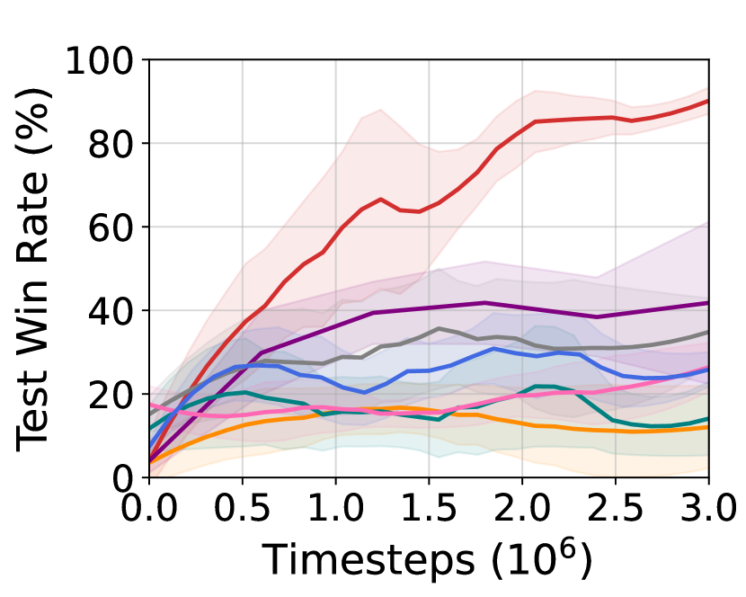
(d) 8m

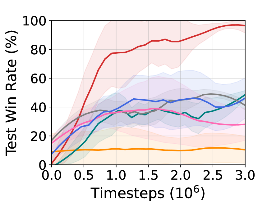
(e) MMM

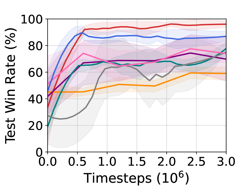
(f) 1c3s5z

Figure E.3: Learning curves of MARL methods for Wolfpack attack across 6 SMAC scenarios (QMIX)

E.3 Performance Comparison for EGA

This section presents the training performance of WALL under the existing Evolutionary Generation-based Attackers (EGA) (Yuan et al., 2023) method across six SMAC scenarios, as shown in Figure E.4. The results demonstrate that WALL consistently achieves superior robustness across all scenarios, even against unseen EGA adversaries that are not included in its training process.

The EGA framework generates a diverse and high-quality population of adversarial attackers. Unlike single-adversary methods, EGA maintains an evolving archive of attackers optimized for both quality and diversity, ensuring robust evaluations against various attack strategies. During training, attackers are randomly selected from the archive to simulate diverse attack scenarios. The archive is iteratively updated by replacing low-quality or redundant attackers with newly generated ones. For evaluation, an attacker policy is randomly selected from the archive. The chosen attacker identifies critical attack steps and targets specific victim agents, introducing action perturbations to reduce their individual $Q$-values. WALL demonstrates strong resilience in these challenging environments, effectively mitigating the impact of EGA adversaries and maintaining high performance across all evaluated scenarios.

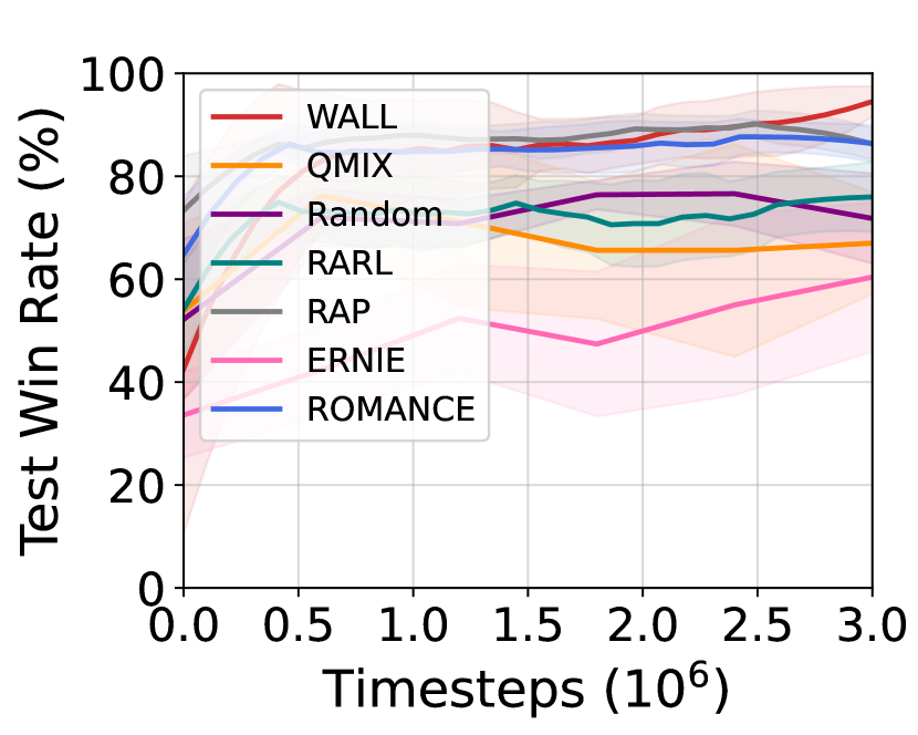
(a) 3m

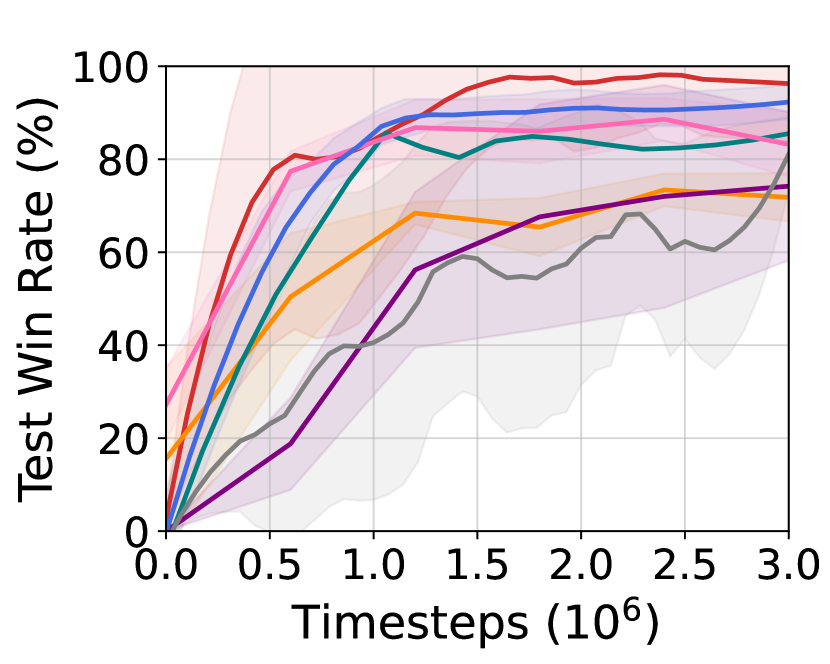
(b) 3s_vs_3z

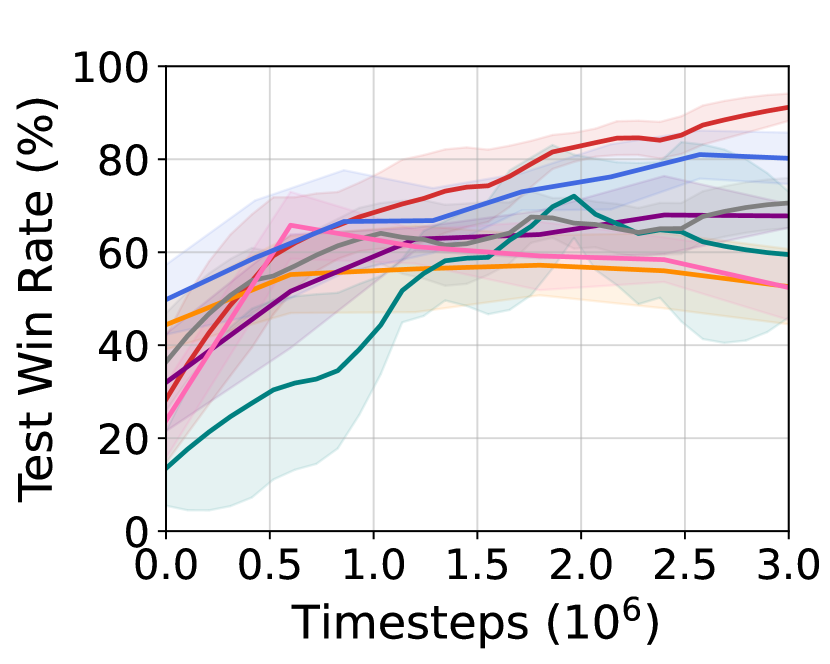
(c) 2s3z

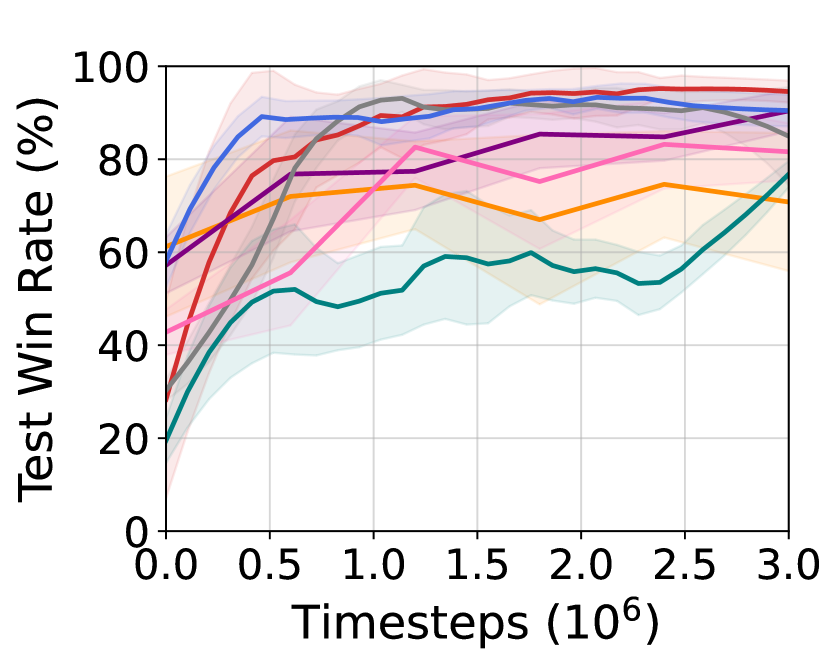
(d) 8m

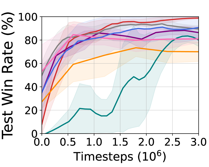
(e) MMM

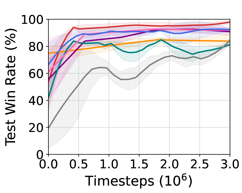
(f) 1c3s5z

Figure E.4: Learning curves of MARL methods for EGA across 6 SMAC scenarios (QMIX)

Appendix F Additional Ablation studies

In this section, we provide additional ablation studies on the number of Wolfpack adversarial attacks $K_{\mathrm{WP}}$ and the attack duration $t_{\mathrm{WP}}$ in the 8m and MMM environments, where the performance differences between WALL and other robust MARL methods are most pronounced.

Number of Wolfpack Attacks $K_{\mathrm{WP}}$: The hyperparameter $K_{\mathrm{WP}}$ determines the number of Wolfpack attacks, with each attack consisting of an initial attack and follow-up attacks over $t_{\mathrm{WP}}=3$ timesteps. The total number of attack steps $K$ for Wolfpack attack is then calculated as $K=4\times K_{\mathrm{WP}}$. In this section, we e conduct a parameter search for $K_{\mathrm{WP}}\in[1,2,3,4]$. Fig. F.1 illustrates the robustness of WALL policies trained with different $K_{\mathrm{WP}}$ values under the default Wolfpack attack in 8m and MMM. In both environments, having too small $K_{\mathrm{WP}}$ results in insufficiently severe attacks, which leads to reduced robustness of the WALL framework. Conversely, in the 8m environment, excessively large $K_{\mathrm{WP}}$ values create overly devastating attacks, making it difficult for CTDE methods to learn strategies to counter the Wolfpack attack, which degrades learning performance. Therefore, an optimal $K_{\mathrm{WP}}$ exists in both environments: $K_{\mathrm{WP}}=2$ for 8m and $K_{\mathrm{WP}}=4$ for MMM, which we choose as the default hyperparameters.

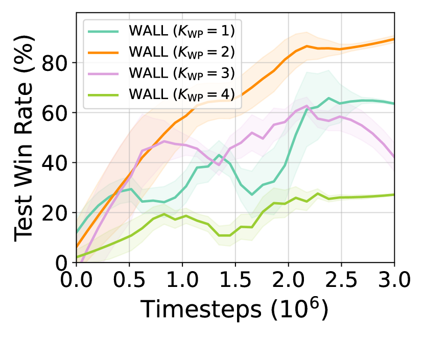
(a) 8m

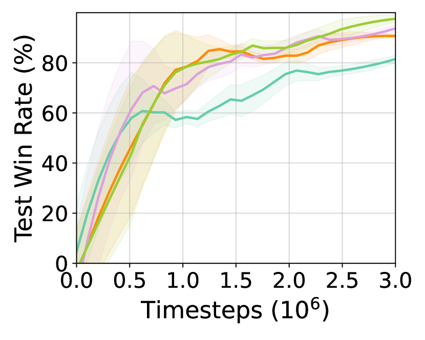
(b) MMM

Figure F.1: Number of Wolfpack Attacks ($K_{\mathrm{WP}}$)

Attack duration $t_{\mathrm{WP}}$: The hyperparameter $t_{\mathrm{WP}}$ determines the duration of follow-up attacks after the initial attack. To analyze its impact on robustness, Fig. F.2 compares performance for $t_{\mathrm{WP}}\in[1,2,3,4]$ in the 8m and MMM environments. As shown in the figure, similar to the case of $K_{\mathrm{WP}}$, setting $t_{\mathrm{WP}}$ too low results in insufficient follow-up attacks on assisting agents, reducing the severity of the attack and lowering the robustness of WALL. On the other hand, excessively high $t_{\mathrm{WP}}$ values lead to overly severe attacks, making it challenging for WALL to learn effective defenses against the Wolfpack attack. Both environments demonstrate that $t_{\mathrm{WP}}=3$ yields optimal performance and is selected as the best hyperparameter.

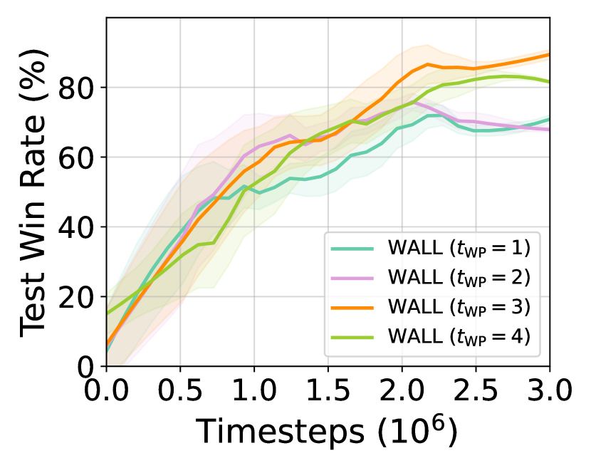
(a) 8m

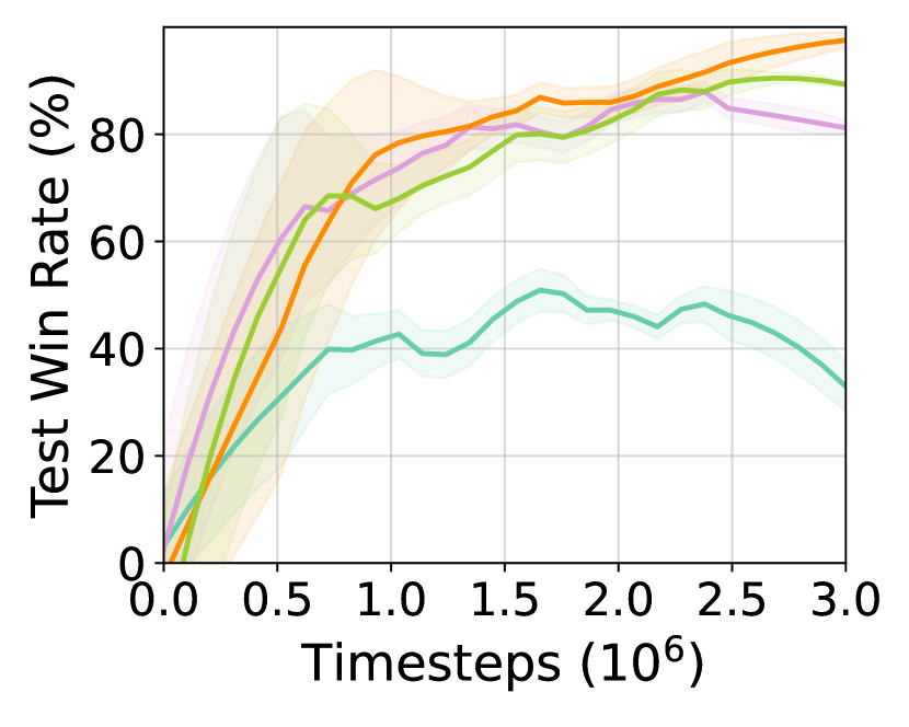
(b) MMM

Figure F.2: Attack duration ($t_{\mathrm{WP}}$)

Appendix G Additional Visualizations of Wolfpack Adversarial Attack

G.1 Visualization of Wolfpack Adversarial Attack Across Additional SMAC Scenarios

To analyze the superior performance of the Wolfpack attack, we provide a visualization of its execution in various SMAC environments. Fig. 7 illustrates the 2s3z task, while Fig. G.1 visualizes the 8m task, and Fig. G.2 presents the MMM task.

Fig. G.1(a) illustrates Vanilla QMIX operating in a natural scenario without any attack, where the agents successfully defeat all enemy units and achieve victory. In this scenario, agents with low health continuously move to the backline to avoid enemy attacks, while agents with higher health position themselves at the frontline to absorb damage. This dynamic coordination enables the team to manage their resources effectively, withstand enemy attacks, and secure a successful outcome.

Fig. G.1(b) depicts Vanilla QMIX under the Wolfpack adversarial attack, where an initial attack is launched at $t=5$, and follow-up agents are targeted between $t=6$ and $t=8$. Agents with higher remaining health are selected as follow-up agents, preventing them from guarding the targeted ally or engaging the enemy effectively. Between $t=10$ and $t=19$, the initial agent continues to take focused enemy fire, eventually succumbing to the attacks and being eliminated. This disruption renders the remaining agents ineffective in defending against the adversarial attack, leading to a loss as all agents are defeated.

Fig. G.1(c) shows the policy trained with the WALL framework. During $t=6$ to $t=8$, the same agents as in (b) are selected as follow-up agents and subjected to the Wolfpack attack, limiting their ability to guard or engage the enemy. Nevertheless, the non-attacked agents adjust by forming a wider formation vertically, effectively dispersing enemy firepower while delivering coordinated attacks. Additionally, agents with higher health move forward to guard the initial agents, ensuring that the initial agents do not die. This tactical adaptation enables the team to eliminate enemy units and secure victory.

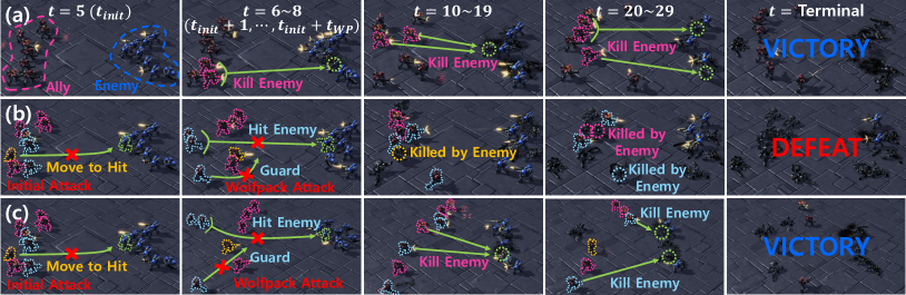
Figure G.1: Attack comparison on 8m task in the SMAC: (a) QMIX/Natural, (b) QMIX/Wolfpack attack, and (c) WALL/Wolfpack attack

Fig. G.2(a) showcases Vanilla QMIX operating in a natural scenario without any adversarial interference, where all enemy units are successfully eliminated, leading to a decisive victory. During this process, agents with lower health retreat to the back while the Medivac agent provides healing, and agents with higher health move forward to absorb enemy attacks. This coordinated strategy enables the team to secure victory efficiently.

Fig. G.2(b) illustrates Vanilla QMIX under the Wolfpack adversarial attack. An initial attack is launched at $t=6$, followed by the targeting of four follow-up agents between $t=7$ and $t=9$. The follow-up agents selected include one healing agent attempting to heal the initial agent, one guarding agent positioned to protect the initial agent, and two agents actively engaging the enemy targeting the initial agent. Due to the Wolfpack attack, the initial agent failed to receive critical healing or guarding support at $t=10$ and $t=19$, leading to its elimination. This disruption severely hindered the remaining agents’ ability to defend against the adversarial attack, ultimately resulting in a loss as all agents are defeated.

Fig. G.2(c) illustrates the policy trained with the WALL framework. During $t=7$ to $t=9$, the same agents as in (b) are selected as follow-up agents and subjected to the Wolfpack attack, restricting their actions such as healing, guarding, or targeting the enemy effectively. However, the non-attacked agents adapt by positioning themselves ahead of the initial agent to provide protection and focus their fire on the enemies targeting the initial agent. This strategic adaptation enables the team to successfully repel the adversarial attack, eliminate enemy units, and secure victory. Notably, in the terminal timesteps, more agents survive under the WALL framework compared to the natural scenario depicted in (a), highlighting the enhanced robustness and stability of the policy learned with WALL.

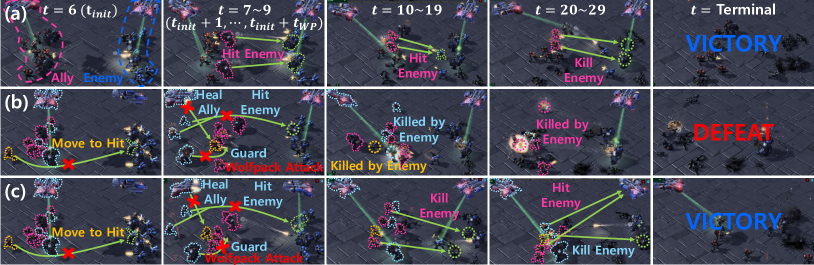
Figure G.2: Attack comparison on MMM task in the SMAC: (a) QMIX/Natural, (b) QMIX/Wolfpack attack, and (c) WALL/Wolfpack attack

G.2 Additional Analysis of Follow-up Agent Group Selection

In this section, we demonstrate that the proposed Follow-up Agent Group Selection method effectively identifies responding agents that protect the initially attacked agent. Fig. G.3 visualizes the process of selecting the follow-up agent group after an initial attack. By comparing the proposed method with a baseline method, Follow-up (L2), which selects $m$ agents closest to the initial agent based on observation L2 distance, we show that our method better identifies responding agents, enabling a more impactful Wolfpack attack.

Fig. G.3(a) illustrates an initial attack on agent $8$, preventing it from performing its original action of hitting the enemy and forcing it to move forward, exposing it to enemy attacks. Fig. G.3(b) shows the Follow-up (L2) method selecting agents $3,4,7,9$ as the follow-up agents based on their proximity to the initial agent. Despite the follow-up attack, non-attacked agents, which is far from the initial agent in terms of observation L2 distance, such as agent $10$, heal the initial agent, while agent $2$ guards it, effectively protecting the initial agent from the attack.

Fig. G.3(c) illustrates the follow-up agents selected using our proposed Follow-up Agent Group Selection method. The selected group includes agents $2$ and $10$, which are responsible for healing and guarding the initial agent, and agents $6$ and $9$, which are hitting enemies targeting the initial agent. These agents are subjected to the follow-up attack, preventing them from performing their protective actions. As a result, the initial agent is left vulnerable, succumbs to enemy attacks, and is ultimately eliminated.

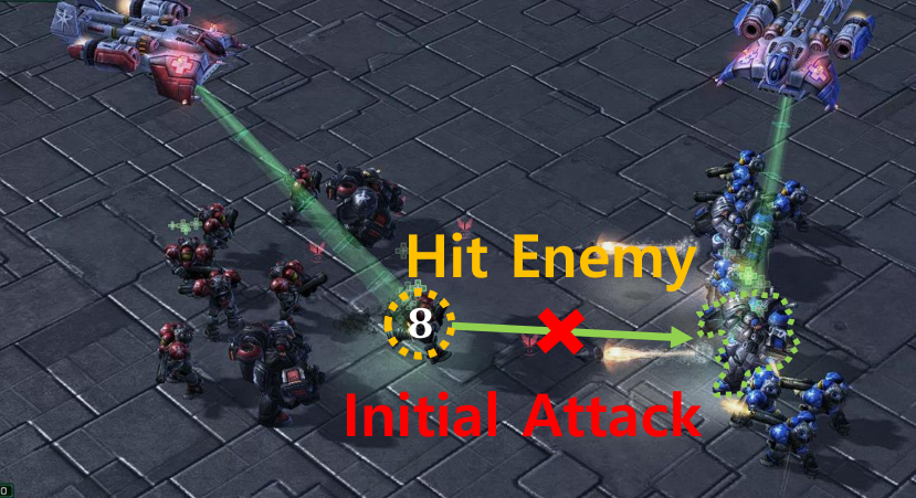
(a) Initial attack

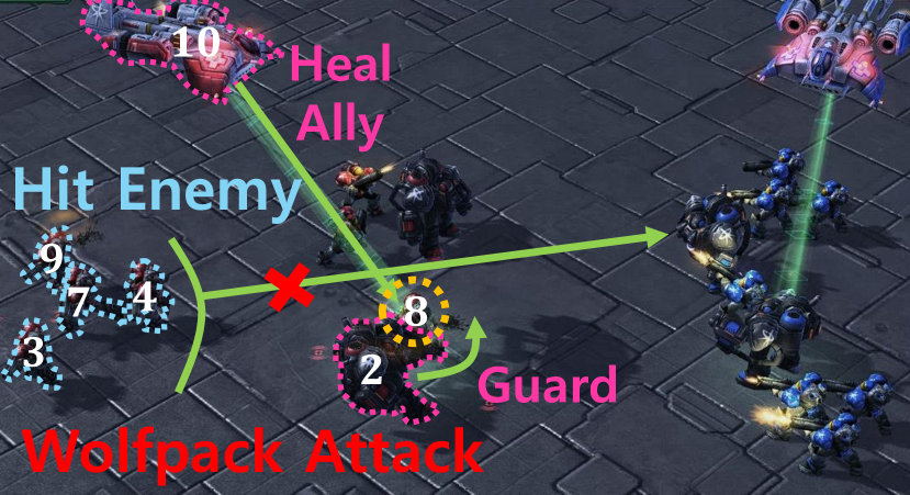
(b) Follow-up (L2)

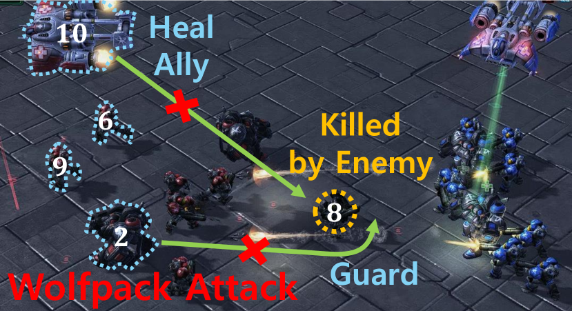
(c) Follow-up Agent Group Selection

Figure G.3: Visualization of follow-up agent group selection comparison for the MMM task in SMAC

Fig. G.4 illustrates the $Soft(Q^{i})$ distribution and the updated $Soft(\tilde{Q}^{i})$ distribution based on Equation 1, highlighting the differences between the two distributions. It is evident that agents $2,6,9,10$ exhibit the largest differences in their distributions. This suggests that, following the initial attack, these agents show noticeable policy changes to adapt and defend against it. Additionally, Fig. G.5 presents the KL divergence values between these two distributions, further confirming that agents $2,6,9,10$ have the highest KL divergence values.

Consequently, based on Equation 2, agents $2,6,9,10$ are selected as the follow-up agent group. This aligns with the visualization results shown in Fig. G.3, demonstrating consistency in the SMAC environment.

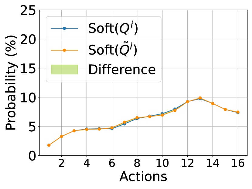
(a) Agent=$1$

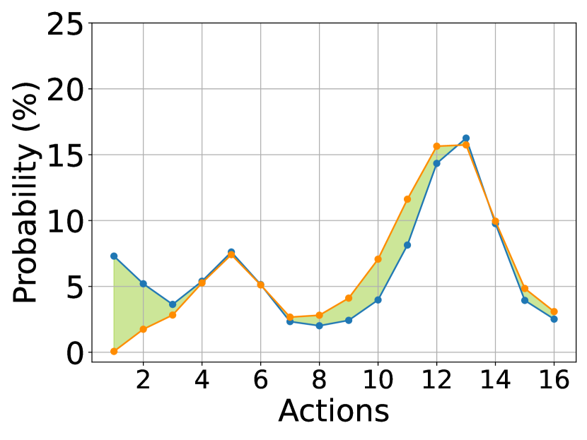
(b) Agent=$2$ (Selected)

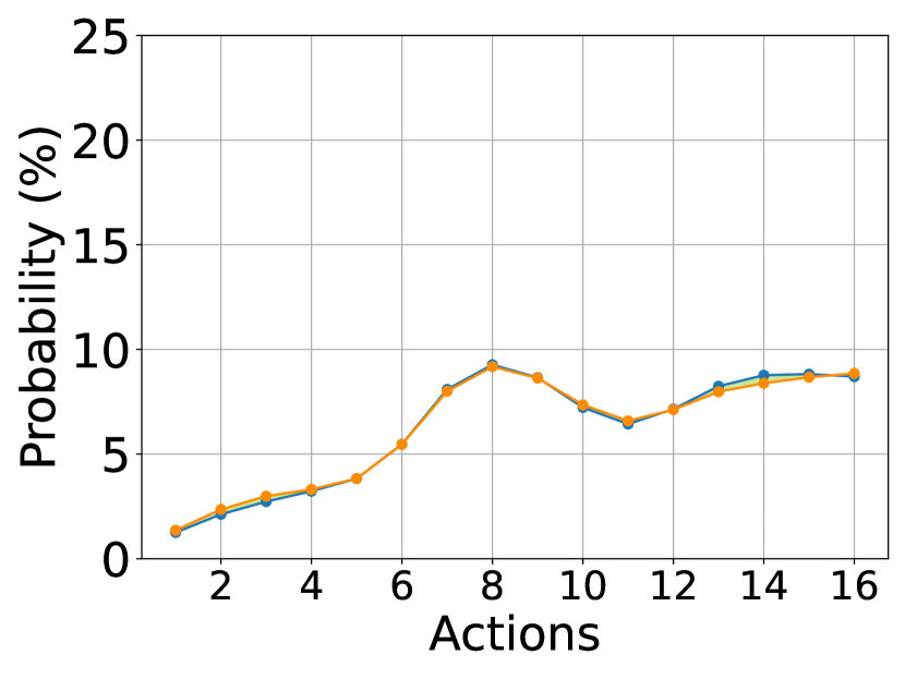
(c) Agent=$3$

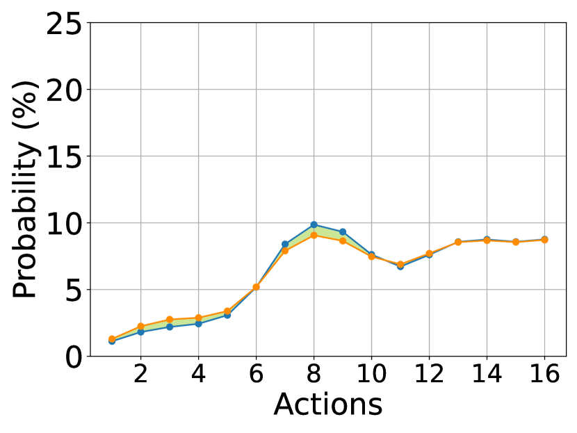
(d) Agent=$4$

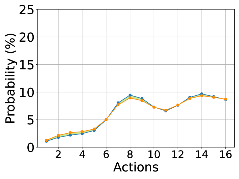
(e) Agent=$5$

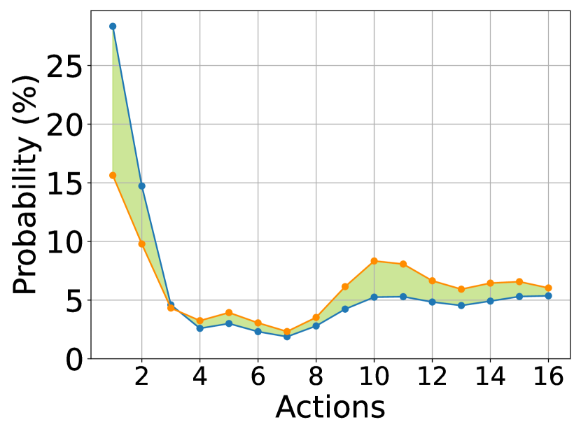
(f) Agent=$6$ (Selected)

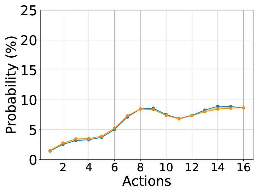
(g) Agent=$7$

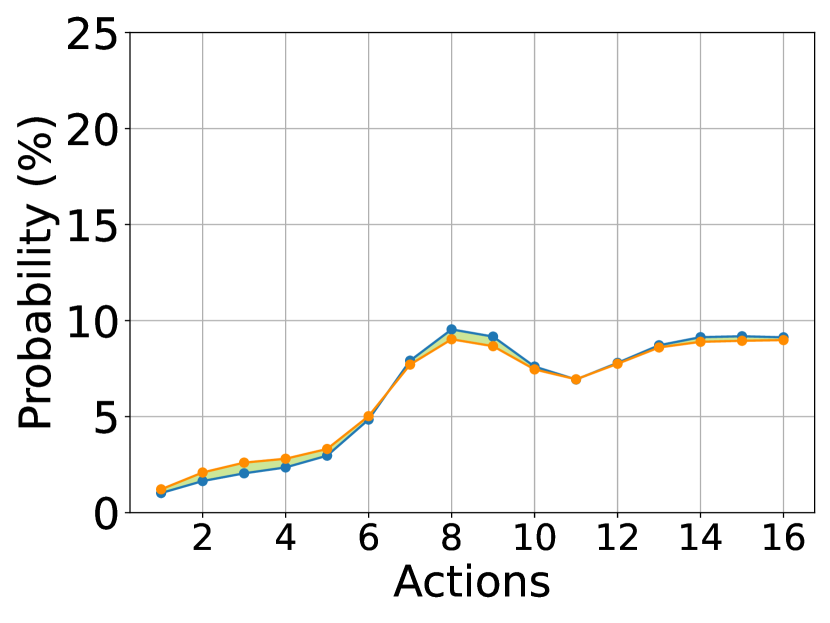
(h) Agent=$8$

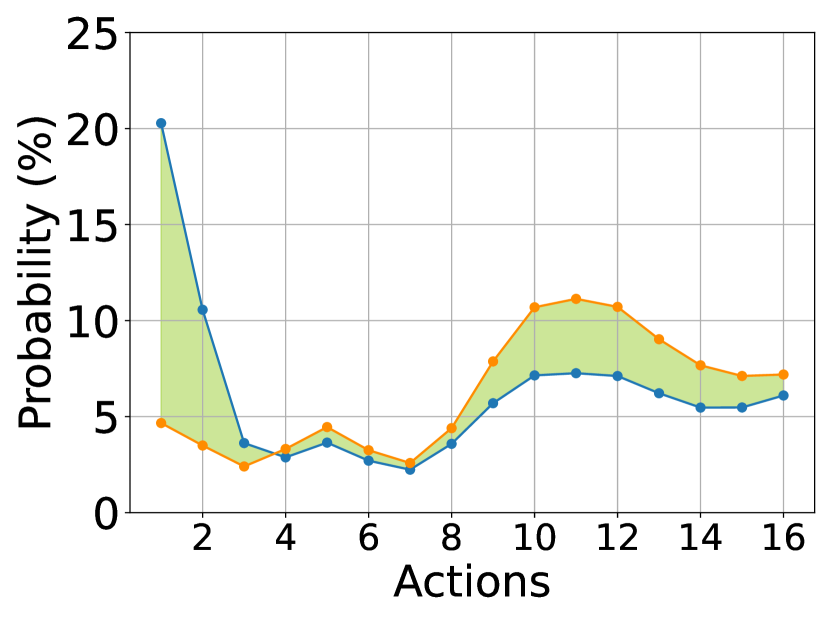
(i) Agent=$9$ (Selected)

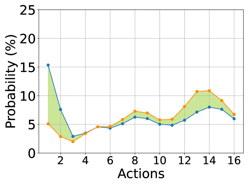
(j) Agent=$10$ (Selected)

Figure G.4: $Soft(Q^{i})$ and $Soft(\tilde{Q}^{i})$ for each agent, along with the difference between the two distributions

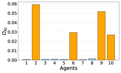
Figure G.5: KL divergence values for each agent, representing the difference between $Soft(Q^{i})$ and $Soft(\tilde{Q}^{i})$ distributions

Appendix H Limitations

The proposed WALL framework effectively defends against the highly detrimental Wolfpack adversarial attack, but it has certain limitations. One drawback is the reliance on complex Transformers for identifying critical steps, which adds computational overhead. However, our method is not strictly dependent on Transformers; any recurrent network capable of generating sequences can be employed in its place. Additionally, while parameter search is required to optimize the Wolfpack attack, the results demonstrate that our method consistently outperforms existing single-agent attack algorithms regardless of parameter choice. Addressing these limitations presents opportunities for further research and improvement.

References

- Berkenkamp et al. (2017) Berkenkamp, F., Turchetta, M., Schoellig, A., and Krause, A. Safe model-based reinforcement learning with stability guarantees. Advances in neural information processing systems, 30, 2017.
- Bhardwaj et al. (2024) Bhardwaj, M., Xie, T., Boots, B., Jiang, N., and Cheng, C.-A. Adversarial model for offline reinforcement learning. Advances in Neural Information Processing Systems, 36, 2024.
- Bouhaddi & Adi (2023) Bouhaddi, M. and Adi, K. Multi-environment training against reward poisoning attacks on deep reinforcement learning. In SECRYPT, pp. 870–875, 2023.
- Bouhaddi & Adi (2024) Bouhaddi, M. and Adi, K. When rewards deceive: Counteracting reward poisoning on online deep reinforcement learning. In 2024 IEEE International Conference on Cyber Security and Resilience (CSR), pp. 38–44. IEEE, 2024.
- Bukharin et al. (2024) Bukharin, A., Li, Y., Yu, Y., Zhang, Q., Chen, Z., Zuo, S., Zhang, C., Zhang, S., and Zhao, T. Robust multi-agent reinforcement learning via adversarial regularization: Theoretical foundation and stable algorithms. Advances in Neural Information Processing Systems, 36, 2024.
- Cai et al. (2023) Cai, K., Zhu, X., and Hu, Z. Reward poisoning attacks in deep reinforcement learning based on exploration strategies. Neurocomputing, 553:126578, 2023.
- Chae et al. (2022) Chae, J., Han, S., Jung, W., Cho, M., Choi, S., and Sung, Y. Robust imitation learning against variations in environment dynamics. In International Conference on Machine Learning, pp. 2828–2852. PMLR, 2022.
- Chen et al. (2023) Chen, J., Ma, R., and Oyekan, J. A deep multi-agent reinforcement learning framework for autonomous aerial navigation to grasping points on loads. Robotics and Autonomous Systems, 167:104489, 2023.
- Chen et al. (2021) Chen, L., Lu, K., Rajeswaran, A., Lee, K., Grover, A., Laskin, M., Abbeel, P., Srinivas, A., and Mordatch, I. Decision transformer: Reinforcement learning via sequence modeling. Advances in neural information processing systems, 34:15084–15097, 2021.
- Chinchuluun et al. (2008) Chinchuluun, A., Migdalas, A., Pardalos, P. M., and Pitsoulis, L. Pareto optimality, game theory and equilibria, volume 17. Springer New York, 2008.
- Clavier et al. (2023) Clavier, P., Pennec, E. L., and Geist, M. Towards minimax optimality of model-based robust reinforcement learning. arXiv preprint arXiv:2302.05372, 2023.
- Curi et al. (2021) Curi, S., Bogunovic, I., and Krause, A. Combining pessimism with optimism for robust and efficient model-based deep reinforcement learning. In International Conference on Machine Learning, pp. 2254–2264. PMLR, 2021.
- Du et al. (2024) Du, X., Chen, H., Wang, C., Xing, Y., Yang, J., Philip, S. Y., Chang, Y., and He, L. Robust multi-agent reinforcement learning via bayesian distributional value estimation. Pattern Recognition, 145:109917, 2024.
- Everett et al. (2021) Everett, M., Lütjens, B., and How, J. P. Certifiable robustness to adversarial state uncertainty in deep reinforcement learning. IEEE Transactions on Neural Networks and Learning Systems, 33(9):4184–4198, 2021.
- Geng et al. (2024) Geng, W., Xiao, B., Li, R., Wei, N., Wang, D., and Zhao, Z. Noise distribution decomposition based multi-agent distributional reinforcement learning. IEEE Transactions on Mobile Computing, 2024.
- Goodfellow et al. (2014) Goodfellow, I. J., Shlens, J., and Szegedy, C. Explaining and harnessing adversarial examples. arXiv preprint arXiv:1412.6572, 2014.
- Guo et al. (2022) Guo, J., Chen, Y., Hao, Y., Yin, Z., Yu, Y., and Li, S. Towards comprehensive testing on the robustness of cooperative multi-agent reinforcement learning. In Proceedings of the IEEE/CVF conference on computer vision and pattern recognition, pp. 115–122, 2022.
- Han & Sung (2021) Han, S. and Sung, Y. A max-min entropy framework for reinforcement learning. Advances in Neural Information Processing Systems, 34:25732–25745, 2021.
- Han et al. (2022) Han, S., Su, S., He, S., Han, S., Yang, H., Zou, S., and Miao, F. What is the solution for state-adversarial multi-agent reinforcement learning? arXiv preprint arXiv:2212.02705, 2022.
- He et al. (2022) He, S., Wang, Y., Han, S., Zou, S., and Miao, F. A robust and constrained multi-agent reinforcement learning framework for electric vehicle amod systems. Dynamics, 8(10), 2022.
- He et al. (2023) He, S., Han, S., Su, S., Han, S., Zou, S., and Miao, F. Robust multi-agent reinforcement learning with state uncertainty. arXiv preprint arXiv:2307.16212, 2023.
- Herremans et al. (2024) Herremans, S., Anwar, A., and Mercelis, S. Robust model-based reinforcement learning with an adversarial auxiliary model. arXiv preprint arXiv:2406.09976, 2024.
- Huang et al. (2017) Huang, S., Papernot, N., Goodfellow, I., Duan, Y., and Abbeel, P. Adversarial attacks on neural network policies. arXiv preprint arXiv:1702.02284, 2017.
- Jendoubi & Bouffard (2023) Jendoubi, I. and Bouffard, F. Multi-agent hierarchical reinforcement learning for energy management. Applied Energy, 332:120500, 2023.
- Jo et al. (2024) Jo, Y., Lee, S., Yeom, J., and Han, S. Fox: Formation-aware exploration in multi-agent reinforcement learning. In Proceedings of the AAAI Conference on Artificial Intelligence, volume 38, pp. 12985–12994, 2024.
- Kardeş et al. (2011) Kardeş, E., Ordóñez, F., and Hall, R. W. Discounted robust stochastic games and an application to queueing control. Operations research, 59(2):365–382, 2011.
- Kobayashi (2024) Kobayashi, T. Lira: Light-robust adversary for model-based reinforcement learning in real world. arXiv preprint arXiv:2409.19617, 2024.
- Lee et al. (2021) Lee, X. Y., Esfandiari, Y., Tan, K. L., and Sarkar, S. Query-based targeted action-space adversarial policies on deep reinforcement learning agents. In Proceedings of the ACM/IEEE 12th international conference on cyber-physical systems, pp. 87–97, 2021.
- Li et al. (2020) Li, R., Wang, R., Tian, T., Jia, F., and Zheng, Z. Multi-agent reinforcement learning based on value distribution. In Journal of Physics: Conference Series, volume 1651, pp. 012017. IOP Publishing, 2020.
- Li et al. (2019) Li, S., Wu, Y., Cui, X., Dong, H., Fang, F., and Russell, S. Robust multi-agent reinforcement learning via minimax deep deterministic policy gradient. In Proceedings of the AAAI conference on artificial intelligence, volume 33, pp. 4213–4220, 2019.
- Li et al. (2023a) Li, S., Guo, J., Xiu, J., Xu, R., Yu, X., Wang, J., Liu, A., Yang, Y., and Liu, X. Byzantine robust cooperative multi-agent reinforcement learning as a bayesian game. arXiv preprint arXiv:2305.12872, 2023a.
- Li et al. (2023b) Li, S., Xu, R., Guo, J., Feng, P., Wang, J., Liu, A., Yang, Y., Liu, X., and Lv, W. Mir2: Towards provably robust multi-agent reinforcement learning by mutual information regularization. arXiv preprint arXiv:2310.09833, 2023b.
- Li et al. (2023c) Li, X., Li, Y., Feng, Z., Wang, Z., and Pan, Q. Ats-o2a: A state-based adversarial attack strategy on deep reinforcement learning. Computers & Security, 129:103259, 2023c.
- Lin et al. (2020) Lin, J., Dzeparoska, K., Zhang, S. Q., Leon-Garcia, A., and Papernot, N. On the robustness of cooperative multi-agent reinforcement learning. In 2020 IEEE Security and Privacy Workshops (SPW), pp. 62–68. IEEE, 2020.
- Liu et al. (2024) Liu, Q., Kuang, Y., and Wang, J. Robust deep reinforcement learning with adaptive adversarial perturbations in action space. arXiv preprint arXiv:2405.11982, 2024.
- Mahajan et al. (2019) Mahajan, A., Rashid, T., Samvelyan, M., and Whiteson, S. Maven: Multi-agent variational exploration. Advances in neural information processing systems, 32, 2019.
- Mankowitz et al. (2019) Mankowitz, D. J., Levine, N., Jeong, R., Shi, Y., Kay, J., Abdolmaleki, A., Springenberg, J. T., Mann, T., Hester, T., and Riedmiller, M. Robust reinforcement learning for continuous control with model misspecification. arXiv preprint arXiv:1906.07516, 2019.
- Moos et al. (2022) Moos, J., Hansel, K., Abdulsamad, H., Stark, S., Clever, D., and Peters, J. Robust reinforcement learning: A review of foundations and recent advances. Machine Learning and Knowledge Extraction, 4(1):276–315, 2022.
- Oliehoek et al. (2008) Oliehoek, F. A., Spaan, M. T., and Vlassis, N. Optimal and approximate q-value functions for decentralized pomdps. Journal of Artificial Intelligence Research, 32:289–353, 2008.
- Oliehoek et al. (2016) Oliehoek, F. A., Amato, C., et al. A concise introduction to decentralized POMDPs, volume 1. Springer, 2016.
- Oroojlooy & Hajinezhad (2023) Oroojlooy, A. and Hajinezhad, D. A review of cooperative multi-agent deep reinforcement learning. Applied Intelligence, 53(11):13677–13722, 2023.
- Orr & Dutta (2023) Orr, J. and Dutta, A. Multi-agent deep reinforcement learning for multi-robot applications: A survey. Sensors, 23(7):3625, 2023.
- Panaganti & Kalathil (2021) Panaganti, K. and Kalathil, D. Sample complexity of model-based robust reinforcement learning. In 2021 60th IEEE Conference on Decision and Control (CDC), pp. 2240–2245. IEEE, 2021.
- Pattanaik et al. (2017) Pattanaik, A., Tang, Z., Liu, S., Bommannan, G., and Chowdhary, G. Robust deep reinforcement learning with adversarial attacks. arXiv preprint arXiv:1712.03632, 2017.
- Phan et al. (2021) Phan, T., Belzner, L., Gabor, T., Sedlmeier, A., Ritz, F., and Linnhoff-Popien, C. Resilient multi-agent reinforcement learning with adversarial value decomposition. In Proceedings of the AAAI Conference on Artificial Intelligence, volume 35, pp. 11308–11316, 2021.
- Pinto et al. (2017) Pinto, L., Davidson, J., Sukthankar, R., and Gupta, A. Robust adversarial reinforcement learning. In International conference on machine learning, pp. 2817–2826. PMLR, 2017.
- Qiaoben et al. (2024) Qiaoben, Y., Ying, C., Zhou, X., Su, H., Zhu, J., and Zhang, B. Understanding adversarial attacks on observations in deep reinforcement learning. Science China Information Sciences, 67(5):1–15, 2024.
- Rakhsha et al. (2021) Rakhsha, A., Zhang, X., Zhu, X., and Singla, A. Reward poisoning in reinforcement learning: Attacks against unknown learners in unknown environments. arXiv preprint arXiv:2102.08492, 2021.
- Ramesh et al. (2024) Ramesh, S. S., Sessa, P. G., Hu, Y., Krause, A., and Bogunovic, I. Distributionally robust model-based reinforcement learning with large state spaces. In International Conference on Artificial Intelligence and Statistics, pp. 100–108. PMLR, 2024.
- Rashid et al. (2020) Rashid, T., Samvelyan, M., De Witt, C. S., Farquhar, G., Foerster, J., and Whiteson, S. Monotonic value function factorisation for deep multi-agent reinforcement learning. Journal of Machine Learning Research, 21(178):1–51, 2020.
- Rigter et al. (2022) Rigter, M., Lacerda, B., and Hawes, N. Rambo-rl: Robust adversarial model-based offline reinforcement learning. Advances in neural information processing systems, 35:16082–16097, 2022.
- Samvelyan et al. (2019) Samvelyan, M., Rashid, T., De Witt, C. S., Farquhar, G., Nardelli, N., Rudner, T. G., Hung, C.-M., Torr, P. H., Foerster, J., and Whiteson, S. The starcraft multi-agent challenge. arXiv preprint arXiv:1902.04043, 2019.
- Shi & Chi (2024) Shi, L. and Chi, Y. Distributionally robust model-based offline reinforcement learning with near-optimal sample complexity. Journal of Machine Learning Research, 25(200):1–91, 2024.
- Shi et al. (2024) Shi, L., Mazumdar, E., Chi, Y., and Wierman, A. Sample-efficient robust multi-agent reinforcement learning in the face of environmental uncertainty. arXiv preprint arXiv:2404.18909, 2024.
- Sun et al. (2023) Sun, Y., Zheng, R., Hassanzadeh, P., Liang, Y., Feizi, S., Ganesh, S., and Huang, F. Certifiably robust policy learning against adversarial multi-agent communication. In The Eleventh International Conference on Learning Representations, 2023.
- Sunehag et al. (2017) Sunehag, P., Lever, G., Gruslys, A., Czarnecki, W. M., Zambaldi, V., Jaderberg, M., Lanctot, M., Sonnerat, N., Leibo, J. Z., Tuyls, K., et al. Value-decomposition networks for cooperative multi-agent learning. arXiv preprint arXiv:1706.05296, 2017.
- Tan et al. (2020) Tan, K. L., Esfandiari, Y., Lee, X. Y., Sarkar, S., et al. Robustifying reinforcement learning agents via action space adversarial training. In 2020 American control conference (ACC), pp. 3959–3964. IEEE, 2020.
- Tessler et al. (2019) Tessler, C., Efroni, Y., and Mannor, S. Action robust reinforcement learning and applications in continuous control. In International Conference on Machine Learning, pp. 6215–6224. PMLR, 2019.
- Tu et al. (2021) Tu, J., Wang, T., Wang, J., Manivasagam, S., Ren, M., and Urtasun, R. Adversarial attacks on multi-agent communication. In Proceedings of the IEEE/CVF International Conference on Computer Vision, pp. 7768–7777, 2021.
- Vaswani (2017) Vaswani, A. Attention is all you need. Advances in Neural Information Processing Systems, 2017.
- Vinitsky et al. (2020) Vinitsky, E., Du, Y., Parvate, K., Jang, K., Abbeel, P., and Bayen, A. Robust reinforcement learning using adversarial populations. arXiv preprint arXiv:2008.01825, 2020.
- Wang et al. (2020a) Wang, J., Liu, Y., and Li, B. Reinforcement learning with perturbed rewards. In Proceedings of the AAAI conference on artificial intelligence, volume 34, pp. 6202–6209, 2020a.
- Wang et al. (2020b) Wang, J., Ren, Z., Liu, T., Yu, Y., and Zhang, C. Qplex: Duplex dueling multi-agent q-learning. arXiv preprint arXiv:2008.01062, 2020b.
- Wang et al. (2023) Wang, S., Chen, W., Huang, L., Zhang, F., Zhao, Z., and Qu, H. Regularization-adapted anderson acceleration for multi-agent reinforcement learning. Knowledge-Based Systems, 275:110709, 2023.
- Wang et al. (2020c) Wang, X., Nair, S., and Althoff, M. Falsification-based robust adversarial reinforcement learning. In 2020 19th IEEE International Conference on Machine Learning and Applications (ICMLA), pp. 205–212. IEEE, 2020c.
- Wang et al. (2022) Wang, Y., Wang, Y., Zhou, Y., Velasquez, A., and Zou, S. Data-driven robust multi-agent reinforcement learning. In 2022 IEEE 32nd International Workshop on Machine Learning for Signal Processing (MLSP), pp. 1–6. IEEE, 2022.
- Xu et al. (2022) Xu, Y., Zeng, Q., and Singh, G. Efficient reward poisoning attacks on online deep reinforcement learning. arXiv preprint arXiv:2205.14842, 2022.
- Xu et al. (2024) Xu, Y., Gumaste, R., and Singh, G. Reward poisoning attack against offline reinforcement learning. arXiv preprint arXiv:2402.09695, 2024.
- Xu et al. (2021) Xu, Z., Li, D., Bai, Y., and Fan, G. Mmd-mix: Value function factorisation with maximum mean discrepancy for cooperative multi-agent reinforcement learning. In 2021 International Joint Conference on Neural Networks (IJCNN), pp. 1–7. IEEE, 2021.
- Xue et al. (2021) Xue, W., Qiu, W., An, B., Rabinovich, Z., Obraztsova, S., and Yeo, C. K. Mis-spoke or mis-lead: Achieving robustness in multi-agent communicative reinforcement learning. arXiv preprint arXiv:2108.03803, 2021.
- Ye et al. (2024) Ye, C., He, J., Gu, Q., and Zhang, T. Towards robust model-based reinforcement learning against adversarial corruption. arXiv preprint arXiv:2402.08991, 2024.
- Yu et al. (2021) Yu, J., Gehring, C., Schäfer, F., and Anandkumar, A. Robust reinforcement learning: A constrained game-theoretic approach. In Learning for Dynamics and Control, pp. 1242–1254. PMLR, 2021.
- Yuan et al. (2023) Yuan, L., Zhang, Z., Xue, K., Yin, H., Chen, F., Guan, C., Li, L., Qian, C., and Yu, Y. Robust multi-agent coordination via evolutionary generation of auxiliary adversarial attackers. In Proceedings of the AAAI Conference on Artificial Intelligence, volume 37, pp. 11753–11762, 2023.
- Yuan et al. (2024) Yuan, L., Jiang, T., Li, L., Chen, F., Zhang, Z., and Yu, Y. Robust cooperative multi-agent reinforcement learning via multi-view message certification. Science China Information Sciences, 67(4):142102, 2024.
- Yun et al. (2022) Yun, W. J., Park, S., Kim, J., Shin, M., Jung, S., Mohaisen, D. A., and Kim, J.-H. Cooperative multiagent deep reinforcement learning for reliable surveillance via autonomous multi-uav control. IEEE Transactions on Industrial Informatics, 18(10):7086–7096, 2022.
- Zhang et al. (2020a) Zhang, H., Chen, H., Xiao, C., Li, B., Liu, M., Boning, D., and Hsieh, C.-J. Robust deep reinforcement learning against adversarial perturbations on state observations. Advances in Neural Information Processing Systems, 33:21024–21037, 2020a.
- Zhang et al. (2021a) Zhang, H., Chen, H., Boning, D., and Hsieh, C.-J. Robust reinforcement learning on state observations with learned optimal adversary. arXiv preprint arXiv:2101.08452, 2021a.
- Zhang et al. (2020b) Zhang, K., Sun, T., Tao, Y., Genc, S., Mallya, S., and Basar, T. Robust multi-agent reinforcement learning with model uncertainty. Advances in neural information processing systems, 33:10571–10583, 2020b.
- Zhang et al. (2021b) Zhang, K., Yang, Z., and Başar, T. Multi-agent reinforcement learning: A selective overview of theories and algorithms. Handbook of reinforcement learning and control, pp. 321–384, 2021b.
- Zhang et al. (2020c) Zhang, X., Ma, Y., Singla, A., and Zhu, X. Adaptive reward-poisoning attacks against reinforcement learning. In International Conference on Machine Learning, pp. 11225–11234. PMLR, 2020c.
- Zhang et al. (2023) Zhang, Z., Sun, Y., Huang, F., and Miao, F. Safe and robust multi-agent reinforcement learning for connected autonomous vehicles under state perturbations. arXiv preprint arXiv:2309.11057, 2023.
- Zhou et al. (2023) Zhou, Z., Liu, G., and Zhou, M. A robust mean-field actor-critic reinforcement learning against adversarial perturbations on agent states. IEEE Transactions on Neural Networks and Learning Systems, 2023.
- Zhou et al. (2024) Zhou, Z., Liu, G., Guo, W., and Zhou, M. Adversarial attacks on multiagent deep reinforcement learning models in continuous action space. IEEE Transactions on Systems, Man, and Cybernetics: Systems, 2024.