On trimming tensor-structured measurements and
efficient low-rank tensor recovery

Abstract.

In this paper, we take a step towards developing efficient hard thresholding methods for low-rank tensor recovery from memory-efficient linear measurements with tensorial structure. Theoretical guarantees for many standard iterative low-rank recovery methods, such as iterative hard thresholding (IHT), are based on model assumptions on the measurement operator, like the restricted isometry property (RIP). However, tensor-structured random linear maps – while memory-efficient and convenient to apply – lack good restricted isometry properties; that is, they do not preserve the norms of low-rank tensors sufficiently well.

To address this, we propose local trimming techniques that provably restore point-wise geometry-preservation properties of tensor-structured maps, making them comparable to those of unstructured sub-Gaussian measurements. Then, we propose two novel versions of tensor IHT algorithms: an adaptive gradient trimming algorithm and a randomized Kaczmarz-based IHT algorithm, that efficiently recover low-rank tensors from linear measurements. We provide initial theoretical guarantees for the proposed methods and present numerical experiments on real and synthetic data, highlighting their efficiency over the original TensorIHT for low HOSVD and CP-rank tensors.

1. Introduction

Tensors, as multi-modal arrays, are natural choices for analyzing realistic high-dimensional structures in a variety of application areas. They have been widely used in recent years for modeling objects in signal processing, medical imaging, machine learning, and other domains [34, 18, 31, 32, 27]. The ubiquity of their applications has motivated the development of specialized techniques to efficiently process large-scale multi-modal data [13, 30, 28]. Due to the large scale of many applications, it is not surprising that the cornerstone techniques in this suite are related to compression and subsequent recovery of tensorial data [40, 24].

Data-oblivious random sketching is a basic and very powerful approach for taming large-scale data. For a given large instance of the data ${\bm{\mathcal{X}}}\in\mathbb{R}^{N}$, the goal is to replace ${\bm{\mathcal{X}}}$ with $\mathcal{A}{\bm{\mathcal{X}}}$ where $\mathcal{A}\in\mathbb{R}^{m\times N}$ is a random matrix with $m\ll N$. Unlike data-aware low-parametric fitting (such as low-rank fitting) which aims to find the best possible approximation for one large and high-dimensional object, selecting a random operator $\mathcal{A}$ allows us to get uniform guarantees for many such large data instances all while avoiding costly fitting procedures. For example, when it is crucial to guarantee the validity of a data sketch through an iterative process, one requires uniform guarantees over all possible iterates.

A key question in oblivious dimensionality reduction is how to design memory-efficient random measurements maps $\mathcal{A}$ that can be applied to the data fast and lead to good compression with high probability [16, 12]. Memory efficiency is especially important for tensorial data, since vectorizing a tensor of dimension $n$ in $d$ modes leads to an object in $\mathbb{R}^{N}$ with $N=n^{d}$, and sketching matrices have to be correspondingly very large-scale. Recent work has studied tensor-specific, fast, and memory-efficient sketching operators. Some key examples include Kronecker (or, modewise) measurements, face-splitting measurements (that consist of independent scalar Kronecker-structured measurements), and more sophisticated tensor-structured measurements are usually built upon the former (an incomplete list includes [51, 44, 50]). In addition to requiring fewer random bits to store structured matrices, these strategies allow fast application to tensor data by mimicking its structure.

The quality of data-oblivious dimension reduction depends on the geometry-preserving properties of the measurement matrices which are often chosen at random. When a linear map satisfies Johnson-Lindenstrauss-type properties, it can be used to reduce dimensionality and speed up a variety of tasks such as clustering and regression [8, 19, 37]. When the goal is the subsequent recovery of the data, the map is usually required to satisfy the Restricted Isometry Property (RIP), which is a uniform guarantee for approximate norm preservation over infinite data sets, such as sparse vectors or low-rank matrices [7]. In this work, we consider the sets of low-rank tensors under some standard notions of tensor rank, specifically, CP and HOSVD.

While RIP properties of generic i.i.d. matrices extend to the low-rank tensor case for various tensor ranks, this is not the situation for memory-efficient measurements. Consequently, it has been observed that popular iterative algorithms such as Iterative Hard Thresholding (IHT) do not work for low-rank tensor recovery from modewise measurements. So, typically, memory-efficient measurements are used within tasks and algorithms that do not require uniform control over the iterates (and where weaker guarantees for the norm preservation suffice), including [49, 58, 51]. Another proposed workaround to get TensorRIP for Kronecker measurements was based on a partial reshaping of the tensor by flattening several modes together [59]. Such a reshaping allowed the Tensor IHT algorithm to successfully recover tensors from memory-efficient measurements. However, the reshaping approach fails to give non-trivial results in an important case of a $3$-mode tensor, as the only option is to flatten all three modes together thus rendering the measurement to no longer be memory efficient. An important motivation for the current work is to give the first nontrivial IHT-like algorithm for $3$-d tensor low-rank recovery from memory-efficient measurements.

In this work, we focus on the following questions: To what extent are the geometry preservation properties of tensorial memory-efficient measurements weaker than that of the standard sub-Gaussian measurement matrices? How can we efficiently run data-oblivious recovery procedures similar to the IHT algorithm for recovery from tensorial measurements? Our main contributions are two-fold:

• RIP-like properties of face-splitting measurements under trimming. We study the limitations of memory-efficient face-splitting measurements as restricted isometry maps and propose adaptive trimming-based local corrections that improve the geometry preservation properties of such operators.

• Efficient iterative hard thresholding variants for low-rank tensor recovery. Motivated by this approach, we propose two new versions of the iterative hard thresholding algorithm for low-rank tensor recovery, TrimTIHT and KaczTIHT, that empirically demonstrate the improved performance for i.i.d. measurements, especially in the hard case of tensor-structured memory-efficient measurements. We also provide convergence theory for the proposed methods giving them initial theoretical validation.

1.1. Paper structure and roadmap.

This paper has the following structure. In Section 2, we review tensor prerequisites and definitions, tensor low-rank recovery problems and their challenges. In Section 3, we focus on memory-efficient tensorial measurements with the face-splitting structure, proving the following

Theorem 1 (Theorem 8 and Proposition 1, informal version).

Let $\bm{A}\in\mathbb{R}^{m\times n^{d}}$ be a matrix with the rows given by Kronecker products of $d$ random vectors in $\mathbb{R}^{n}$ with i.i.d. mean zero, variance one, sub-Gaussian entries. Then, for the set $\mathcal{S}$ of all unit norm tensors of HOSVD rank at most $(r,\ldots,r)$, we have with probability $1-cn^{-\phi}$,

(1) $$\sup_{{\bm{\mathcal{Y}}}\in\mathcal{S}}\left|\|\bm{A}^{\bm{y}}{\bm{y}}\|_{2}^{2}-1\right|\leq\delta\;,$$

as long as $m\gtrsim\delta^{-2}d(r^{d}+dnr){\ln(n/\delta)}$. Here, $\bm{A}^{\bm{y}}$ is a version of $\bm{A}$ without $\ln(8n^{\phi})$ rows that are most aligned with ${\bm{y}}=\textnormal{{Vec}}({\bm{\mathcal{Y}}})$. If $\mathcal{S}$ denotes the set of all norm-$1$ tensors of CP-rank at most $r$, the same holds for $m\gtrsim\delta^{-2}d^{2}nr{\ln(n/\delta)}$. However, if we do not remove any rows, that is, we try to get a standard RIP guarantee for the set low-rank tensors, then we fail essentially with any nontrivial amount of compression: for any $\alpha>0$, the probability of (1) with $\bm{A}^{\bm{y}}=\bm{A}$ goes to zero for any $m<n^{d(1-\alpha)}$.

Then, in Section 4, we propose new variants of TensorIHT algorithm that are applicable to general, and not necessarily face-splitting, linear measurements. Informally, the original IHT algorithm alternates gradient steps with sparse (or low-rank) fitting. In Algorithm 1, TrimTIHT, we replace the gradient step of the TIHT algorithm with a scaled gradient estimate calculated based on a subset of rows of $\bm{A}$, chosen adaptively to the current iterate as to enhance its norm preservation properties. To analyze the convergence of the method, we develop a path-based analysis of the convergence of TensorIHT, see Theorem 10. Then, in Remark 5, we discuss why our trimming results, such as Theorem 1, suggest the advantages of TrimTIHT on the face-splitting measurements.

The idea of the second proposed algorithm, KaczTIHT (Algorithm 2), is to substitute the gradient step with a sequence of stochastic gradient steps, thereby employing the convergence properties of the Kaczmarz linear solver [2, 10]. This is a multi-order extension of the recently proposed [22] and analyzed [60] Kaczmarz Iterative Hard Thresholding method. We also provide a convergence guarantee for the KaczTIHT method, however under the stronger assumptions of i.i.d. sub-Gaussian measurements.

Then, in Section 5 we demonstrate empirically the advantages of the proposed methods, that are especially pronounced in less regular measurements, such as memory-efficient face-splitting measurements. We conclude and discuss the future directions of this work in Section 6.

2. Preliminaries and Related Work

Throughout this paper, we adopt the following notations: the bold calligraphic font (e.g. ${\bm{\mathcal{X}}},{\bm{\mathcal{Y}}}$) is dedicated solely to tensors, the capital Roman script (e.g. $\bm{X},\bm{Y}$) is for matrices and the bold lower case (e.g ${\bm{x}},{\bm{y}}$) is for vectors. The element of the tensor ${\bm{\mathcal{X}}}$ corresponding to the multi-index ${\bm{i}}=(i_{1},i_{2},\dots i_{d})\in[n_{1}]\times[n_{2}]\dots[n_{d}]$, is denoted by either ${\bm{\mathcal{X}}}(\bm{i})$ or ${\bm{\mathcal{X}}}_{i_{1}i_{2}\dots i_{d}}$. For two real functions $f,g$, we say that $f=O(g)$ if $|f(x)|\leq M|g(x)|$ for all $x>c$, for some $M$ and $c\in\mathbb{R}^{+}$. We will also use $\|\bm{A}\|_{2}$ to denote the operator norm of a matrix $\bm{A}\in\mathbb{R}^{m\times n}$ that is given by $\sup_{{\bm{v}}\in\mathbbm{S}^{n-1}}{\|\bm{A}{\bm{v}}\|_{2}}$. Here and further, let $\mathbbm{S}^{n-1}$ denote the unit sphere in $\mathbb{R}^{n}$.

2.1. Tensor preliminaries

For an in-depth overview of tensor-related concepts, we refer to [63, 9]. Here, we include and briefly discuss the notions crucial for this paper.

Reshaping. By collapsing the tensor along all modes, we can uniquely map the tensor ${\bm{\mathcal{X}}}~\in~\mathbb{R}^{n_{1}\times n_{2}\dots n_{d}}$ to a vector ${\bm{x}}\in\mathbb{R}^{n_{1}n_{2}\dots n_{d}}$. Let this map be denoted by

$$\textnormal{{Vec}}:\mathbb{R}^{n_{1}\times n_{2}\dots\times n_{d}}\rightarrow\mathbb{R}^{n_{1}n_{2}\dots n_{d}}.$$

Inner Product and Norm. The inner product and Frobenious norm of the tensors ${\bm{\mathcal{X}}},{\bm{\mathcal{Y}}}\in\mathbb{R}^{n_{1}\times n_{2}\dots\times n_{d}}$ are defined as the inner product and Euclidean norm of their respective vectorisations:

$$\langle{\bm{\mathcal{X}}},{\bm{\mathcal{Y}}}\rangle=\langle\textnormal{{Vec}}({\bm{\mathcal{X}}}),\textnormal{{Vec}}({\bm{\mathcal{Y}}})\rangle\text{ and }\quad\|{\bm{\mathcal{X}}}\|_{F}=\sqrt{\langle{\bm{\mathcal{X}}},{\bm{\mathcal{X}}}\rangle}=\|\textnormal{{Vec}}({\bm{\mathcal{X}}})\|_{2}\;.$$

Mode-wise product. A key operation on tensors is their modewise multiplication with matrices. Given a tensor ${\bm{\mathcal{X}}}\in\mathbb{R}^{n_{1}\times n_{2}\dots\times n_{d}}$, its $k$-mode tensor product with a matrix $\bm{A}\in\mathbb{R}^{m\times n_{k}}$, denoted by ${\bm{\mathcal{X}}}\times_{k}\bm{A}\in\mathbb{R}^{n_{1}\times\dots n_{k}\times m\times n_{k+1}\dots n_{d}}$, is given entry-wise by

$$({\bm{\mathcal{X}}}\times_{k}\bm{A})_{i_{1}i_{2}\dots i_{k}\dots i_{d}}=\sum_{j=1}^{n_{k}}{\bm{\mathcal{X}}}_{i_{1}\dots i_{k-1}ji_{k+1}\dots i_{d}}\bm{A}_{i_{k}j}\;.$$

Rank-1 tensor. ${\bm{\mathcal{X}}}\in\mathbb{R}^{n_{1}\times n_{2}\dots\times n_{d}}$ is said to be a rank one tensor if it can be expressed as

(2) $$\ \ {\bm{\mathcal{X}}}={\bm{x}}_{1}\bigcirc{\bm{x}}_{2}\dots\bigcirc{\bm{x}}_{d},\quad\text{ or }\quad({\bm{\mathcal{X}}})_{i_{1}i_{2}\dots i_{k}\dots i_{d}}=({\bm{x}}_{1})_{i_{1}}({\bm{x}}_{2})_{i_{2}}\dots({\bm{x}}_{d})_{i_{d}},$$

where $\bigcirc$ denotes vector outer product and the vectors ${\bm{x}}_{i}\in\mathbb{R}^{n_{i}}$ for $i=1,\ldots,d$. If ${\bm{\mathcal{X}}}$ is a rank-1 tensor, the mode-wise product of ${\bm{\mathcal{X}}}$ with any matrix $\bm{A}\in\mathbb{R}^{m\times n_{k}}$ can be elegantly written in terms of its components ${\bm{x}}_{i}$ as-

$${\bm{\mathcal{X}}}\times_{k}\bm{A}=\left(\bigcirc_{i=1}^{k-1}{\bm{x}}_{i}\right)\bigcirc\bm{A}{\bm{x}}_{k}\bigcirc\left(\bigcirc_{i=k+1}^{d}{\bm{x}}_{i}\right).$$

Tensor Decompositions and Tensor Rank. Extending the definition of tensor rank from rank 1 to rank $k$ for $k>1$ has significant difficulties, resulting in multiple definitions of tensor rank. Two of the most natural notions of tensor rank that are considered in this paper are

1. [CP] A tensor ${\bm{\mathcal{X}}}\in\mathbb{R}^{n_{1}\times n_{2}\dots n_{d}}$ is said to be of CP rank-$r$ if it can be expressed as a sum of $r$ rank-1 tensors. That is, if $\exists\ {\bm{x}}_{ij}\in\mathbb{R}^{n_{i}}$ for all $i\in[d]$ and $j\in[r]$ such that

   $${\bm{\mathcal{X}}}=\sum_{j=1}^{r}{\bm{x}}_{1j}\bigcirc{\bm{x}}_{2j}\dots\bigcirc{\bm{x}}_{dj}\;.$$

   While this decomposition of a tensor into vectors is very convenient, such minimal $r$ is NP-hard to find or even verify for a given tensor, also, one cannot guarantee even approximate orthogonality of the factor vectors. This motivates alternate definitions of the tensor rank.

2. [HOSVD] Given a tensor ${\bm{\mathcal{X}}}\in\mathbb{R}^{n_{1}\times\dots\times n_{d}}$, the Tucker decomposition of ${\bm{\mathcal{X}}}$ consists of a core tensor ${\bm{\mathcal{C}}}\in\mathbb{R}^{r_{1}\times\dots\times r_{d}}$ and matrices $\bm{U}_{i}\in\mathbb{R}^{n_{i}\times r_{i}}$ for $i\in[d]$ where

   $${\bm{\mathcal{X}}}={\bm{\mathcal{C}}}\times_{1}\bm{U}_{1}\times_{2}\dots\times_{d}\bm{U}_{d}\;.$$

   If for all $i\in[d]$, the columns of the matrix $\bm{U}_{i}$ form an orthonormal basis, this decomposition is known as the Higher-Order Singular Value Decomposition. The HOSVD (or Tucker) rank of ${\bm{\mathcal{X}}}$ is given by ${\bm{r}}=(r_{1},r_{2},\dots,r_{d})$, the dimension of the core tensor ${\bm{\mathcal{C}}}$. Furthermore, the HOSVD decomposition can be chosen such that the core-tensor has orthogonal sub-tensors. More formally, let ${\bm{\mathcal{Q}}}_{k_{i}=p}\in\mathbb{R}^{n_{1}\times n_{2}\dots n_{i-1}\times n_{i+1}\dots n_{d}}$ denote the $(d-1)$-order sub-tensor obtained by fixing the $i$-mode coordinate to $p$ for some $i\in[d]$. Then, for $p\neq q$,

   $$\langle{\bm{\mathcal{Q}}}_{k_{i}=p},{\bm{\mathcal{Q}}}_{k_{i}=q}\rangle=0\;.$$

Various domain-specific applications have motivated the definition of different notions of tensor rank that are beyond the scope of this paper, see, e.g., [63] fo further discussion.

Low-Rank Tensor Fitting. Unlike the matrix setting, where the Eckart-Young theorem gives us a direct way to obtain the best rank-$k$ approximation using SVD [1], such guarantees are not as straightforward for higher-order tensors. In fact, under the CP setting, the best rank $k$-approximation might not exist, and even when it does, is NP-hard to compute [5].

In [43], the authors proposed randomized algorithms for low-rank fitting that are poly-time in the dimensions of the tensor as follows. For simplicity, let us state the results for the tensors with the same dimension in each mode.

Theorem 2 (Low CP Rank Approximation [43, Theorem 1.2]).

Given an order $d$ tensor ${\bm{\mathcal{X}}}$ in $\mathbb{R}^{n\times n\dots\times n}$ and $\varepsilon>0$ , let

$$\textnormal{{Opt}}=\underset{{\bm{\mathcal{Y}}}-\text{CP rank r}}{\min}\|{\bm{\mathcal{X}}}-{\bm{\mathcal{Y}}}\|^{2}_{F}.$$

If there exists $\delta>0$ and ${\bm{\mathcal{X}}}_{r}~=~\sum_{j=1}^{r}~{\bm{x}}_{1j}~\bigcirc~{\bm{x}}_{2j}~\dots~\bigcirc~{\bm{x}}_{dj}$ such that $\|{\bm{x}}_{ij}\|\leq 2^{O(n^{\delta})}$ for all $i\in[d]$ and $j\in[r]$ and $\|{\bm{\mathcal{X}}}-{\bm{\mathcal{X}}}_{r}\|_{F}^{2}\leq\textnormal{{Opt}}+2^{-O(n^{\delta})}$, then a proposed algorithm outputs a rank $r$-tensor ${\bm{\mathcal{Z}}}$ such that

$$\|{\bm{\mathcal{Z}}}-{\bm{\mathcal{X}}}\|^{2}_{F}\leq(1+\varepsilon)\textnormal{{Opt}}+2^{-O(n^{\delta})}\;.$$

Further, this algorithm runs in $O\left(n^{d+\delta}+n^{\delta+1}\text{poly}(r,1/\varepsilon)+n^{\delta}2^{O\left(\text{poly}(r,1/\varepsilon)\right)}\right)$ time.

Theorem 3 (Low HOSVD Rank Approximation [43, Theorem L.2]).

Given an order $d$ tensor ${\bm{\mathcal{X}}}\in\mathbb{R}^{n\times n\times\dots\times n}$ and $\varepsilon>0$, there exists an algorithm that outputs a HOSVD rank ${\bm{r}}=(r,r,\dots,r)$ tensor ${\bm{\mathcal{Z}}}$ such that,

$$\|{\bm{\mathcal{Z}}}-{\bm{\mathcal{X}}}\|_{F}^{2}\leq(1+\varepsilon)\|{\bm{\mathcal{X}}}-{\bm{\mathcal{X}}}_{best}\|_{F}^{2}\;,$$

where ${\bm{\mathcal{X}}}_{best}$ is the best HOSVD-rank ${\bm{r}}$ approximation of ${\bm{\mathcal{X}}}$. Further, the running time of this algorithm is $O\left(n^{d}+n\text{poly}(r,1/\varepsilon)+2^{O\left(\text{poly}(r,1/\varepsilon)\right)}\right)$.

These algorithms, while providing good approximation guarantees, have added assumptions for CP rank and they are computationally expensive to run. In the standard tensor packages, variants of the alternating least squares algorithm are used to compute a CP rank-$k$ approximation to any given tensor [35]. Similarly, for low-rank Tucker approximation, the commonly used algorithms include the Higher Order Orthogonal Iterations (HOOI), HOSVD and ST-HOSVD [3, 14]. Both HOSVD and ST-HOSVD are, $\sqrt{d}$-quasi-optimal. That, is given a tensor ${\bm{\mathcal{X}}}$, the rank-${\bm{r}}$ output of these algorithms, $\bar{{{\bm{\mathcal{X}}}}}$ satisfies -

(3) $$\|{\bm{\mathcal{X}}}-\bar{{\bm{\mathcal{X}}}}\|_{F}\leq\sqrt{d}\|{\bm{\mathcal{X}}}-{\bm{\mathcal{X}}}_{best}\|_{F}\;,$$

where ${\bm{\mathcal{X}}}_{best}$ is the optimal rank-${\bm{r}}$ approximation. The HOOI algorithm often gives better approximation guarantees in practice. However, it can be accompanied by increased computational and storage costs [4] depending on the number of iterations. For the experiments described in this paper, we use CP-ALS and HOOI from the Tensorly package [42] in Python for low rank CP and Tucker approximation respectively.

It is pertinent to note that results such as (3) are worst case bounds and in practice, these methods provide better approximations for most instances. This gap between theory and observations led authors to assume a better bound on this approximation in some works, e.g., [33] (see more detailed discussion in Section 2.3 below). In our theoretical analysis, we will adopt similar assumptions for the low-rank approximation operator.

2.2. RIP and geometry preserving linear operators

A standard way to capture the ability of some operator $\mathcal{A}$ to preserve geometric properties of the objects from a class is through the restricted isometry property:

Definition 2.1.

[$(\delta,\mathcal{S})$-Restricted Isometry Property (RIP)] A measurement operator $\mathcal{A}:\mathcal{S}\rightarrow\mathbb{R}^{m}$ satisfies $(\delta,{\mathcal{S})}$-RIP if

$$(1-\delta)\|{\bm{s}}\|^{2}\leq\|\mathcal{A}({\bm{s}})\|^{2}\leq(1+\delta)\|{\bm{s}}\|^{2}\quad\forall{\bm{s}}\in\mathcal{S}\;.$$

Informally, RIP guarantees that the sketching with $\mathcal{A}$ approximately preserves the norm of all objects within the set of interest $\mathcal{S}$. Depending on the task, $\mathcal{S}$ can be an arbitrary finite set (then Definition 2.1 reduces to the classical Johnson-Lindenstrauss property), or an unknown low-dimensional subspace (then it is known as the Oblivious Subspace Embedding property), or any collection of objects of low-complexity, such as, all sparse vectors or all matrices of low-rank $r$. The latter case is the standard interpretation of the RIP property. Here, we are interested in the sets of all low-rank tensors as so we call the corresponding property TensorRIP:

Definition 2.2 (TensorRIP).

Let’s denote the sets of low-rank tensors as follows

$$\mathcal{S}_{\bm{r}}^{HOSVD}=\left\{{\bm{\mathcal{X}}}\in\mathbb{R}^{n_{1}\times n_{2}\dots\times n_{d}}\ |\ \text{HOSVD Rank}({\bm{\mathcal{X}}})={\bm{r}}=(r_{1},r_{2}\dots r_{d}),\ \|{\bm{\mathcal{X}}}\|_{F}=1\right\},$$

$$\mathcal{S}_{r}^{CP}=\left\{{\bm{\mathcal{X}}}\in\mathbb{R}^{n_{1}\times n_{2}\dots n_{d}}\ |\ \text{CP Rank}({\bm{\mathcal{X}}})=r,\ \|{\bm{\mathcal{X}}}\|_{F}=1\right\},$$

and the $(\delta,\mathcal{S}_{\bm{r}}^{HOSVD})$-RIP will be further denoted as $(\delta,\mathbf{r})$-TensorRIP property for brevity, while $(\delta,\mathcal{S}_{r}^{CP})$-RIP will be denoted as $(\delta,r)$-TensorRIP.

A key for RIP to hold over some set $\mathcal{S}$ is in bounding of the intrinsic complexity of the set, and one of the standard ways to do so is via the covering number:

Definition 2.3 ($\varepsilon$-net and Covering Number).

Consider a subset $K$ of a metric space $(T,d)$, and let $\varepsilon>0$. Then, a set $\mathcal{N}\subseteq K$ is said to be an $\varepsilon$-net of $K$ if for any ${\bm{x}}\in K$, there exists ${\bm{x}}^{\prime}\in K$ such that $d({\bm{x}},{\bm{x}}^{\prime})\leq\varepsilon.$ Further, the covering number of $K$, denoted by $\mathcal{N}(K,d,\varepsilon)$, is the smallest possible cardinality of an $\varepsilon$-net of $K$.

Remark 1 (Covering numbers for low-rank tensors).

The following upper bounds for covering numbers for the sets ${\mathcal{S}}_{\bm{r}}^{HOSVD}$ and ${\mathcal{S}}_{r}^{CP}$ are known. For any $\varepsilon\in(0,1)$ are given by,

$$\ln\mathcal{N}({\mathcal{S}}_{\bm{r}}^{HOSVD},\|.\|_{F},\varepsilon)\leq({r_{1}r_{2}\dots r_{d}+\sum_{i=1}^{d}n_{i}r_{i}})\ln\left(\frac{3(d+1)}{\varepsilon}\right)\text{\cite[cite]{[\@@bibref{}{rauhut2017low}{}{}]}},$$

$$\ln\mathcal{N}({\mathcal{S}}_{r}^{CP},\|.\|_{F},\varepsilon)\leq C\left(r\sum_{i=1}^{d}n_{i}\ln\left(\frac{n_{1}n_{2}\dots n_{d}}{\varepsilon}\right)\right)\text{\cite[cite]{[\@@bibref{}{zhang2023covering}{}{}]}}.$$

for some constant $C>0$. The logarithm of the covering numbers $\ln\mathcal{N}(K,\epsilon)$ is often called the metric entropy of $K$. It is known (e.g., [36]) that the metric entropy is equivalent to the number of bits needed to encode points in $K$. Note that the set of $d$-mode HOSVD rank-${\bm{r}}$ tensors needs $r_{1}r_{2}\dots r_{d}+\sum_{i=1}^{d}n_{i}r_{i}$ bits to encode it, so the estimate above is $(\ln d)$-optimal. Similarly, for CP rank-$r$ tensors, $r\sum_{i=1}^{d}n_{i}$ bits is enough, and the estimate from [62] is optimal up to an extra $d\ln{n}$ factor. The estimates without this extra factor are available (and are much easier to get) under additional conditions like bounded factors or incoherence [57, 46].

2.3. Low-rank tensor recovery and Iterative Hard Thresholding algorithm

The low-rank tensor recovery problem aims to find an unknown $d$-dimensional tensor ${\bm{\mathcal{X}}}\in\mathbb{R}^{n_{1}\times n_{2}\dots n_{d}}$ from $m$ possibly noisy measurements ${\bm{b}}=\mathcal{A}({\bm{\mathcal{X}}})+\bm{\eta}\in\mathbb{R}^{m}$ of a linear measurement operator $\mathcal{A}:\mathbb{R}^{n_{1}\times n_{2}\dots n_{d}}~\to~\mathbb{R}^{m}$, where typically, $m\ll n_{1}n_{2}\dots n_{d}$, and the noise vector $\bm{\eta}$ is assumed to have a small norm. This is a higher-order extension of a classical problem of sparse vector and low-rank matrix recovery. The recovery guarantees of structured objects from a small number of linear measurements can be established under some assumptions on the measurement matrix including RIP [6]. Various algorithms have been employed to solve the low-rank matrix recovery problem [25, 26, 15, 29]. Some of these methods have been extended to the tensor setting as well [33, 61]. In this paper, we consider a particular example of one of the simplest algorithms, iterative hard thresholding. Iterative thresholding based algorithms are incredibly effective in solving low-rank matrix [11] and tensor recovery [57, 20] problems. Moreover, the simplicity of this method enables us to modify or adapt it to different settings [45, 21, 52].

The tensor iterative hard thresholding (TIHT) algorithm is given by the following iterative steps, starting from some initialization ${\bm{\mathcal{X}}}^{0}$:

$${\bm{\mathcal{Y}}}^{j+1}={\bm{\mathcal{X}}}^{j}+\mu_{j}\mathcal{A}^{*}({\bm{b}}-\mathcal{A}({\bm{\mathcal{X}}}^{j}))\quad\forall j\geq 1\;,$$

$${\bm{\mathcal{X}}}^{j+1}=T_{{\bm{r}}}({\bm{\mathcal{Y}}}^{j+1})\;.$$

Here, $T_{\bm{r}}$ denotes a low-rank approximation operator (which can be realized in a number of ways as we discussed in Section 2.1), $\mu_{j}\in\mathbb{R}^{+}$ represents the step size and $\mathcal{A}^{*}$ denotes the adjoint of $\mathcal{A}$. It is known that this algorithm converges under TensorRIP assumptions on the measurement operator $\mathcal{A}$, specifically,

Theorem 4 (TIHT for Low Rank Recovery [33]).

Let $\mathcal{A}:\mathbb{R}^{n_{1}\times n_{2}\dots\times n_{d}}\rightarrow\mathbb{R}^{m}$ be a measurement operator satisfying $(\delta,{3\textbf{r}})$-TensorRIP with $\delta_{3{\bm{r}}}<\frac{a}{4}$ for some $a\in(0,1)$. Also, let ${\bm{\mathcal{X}}}\in\mathbb{R}^{n_{1}\times n_{2}\dots\times n_{d}}$ be a low rank-$\mathbf{r}$ tensor for some notion of tensor rank and ${\bm{b}}=\mathcal{A}({\bm{\mathcal{X}}})+\bm{\eta}$ be (noisy) measurements of ${\bm{\mathcal{X}}}$. Further, let’s assume that each iteration of TIHT satisfies

(4) $$\|{\bm{\mathcal{Y}}}^{j}-{\bm{\mathcal{X}}}^{j+1}\|_{F}\leq\left(1+\frac{a^{2}}{17(1+\sqrt{1+\delta})^{2}}\right)\|{\bm{\mathcal{Y}}}^{j}-{\bm{\mathcal{X}}}\|_{F}.$$

Then the iterates of the TIHT algorithm with the step size one satisfy

$$\|{\bm{\mathcal{X}}}-{\bm{\mathcal{X}}}^{j+1}\|_{F}\leq a^{j}\|{\bm{\mathcal{X}}}-{\bm{\mathcal{X}}}^{0}\|_{F}+\frac{\xi(a)}{1-a}\|\bm{\eta}\|_{2}\quad\text{ for all }j\in\mathbb{N},$$

where

$$\xi(a)=2\sqrt{1+\delta}+\sqrt{4\sigma(a)+2\sigma(a)^{2}}\frac{1}{1-\delta}{\|\bm{A}\|_{2}} \sigma(a)=\frac{a^{2}}{17(1+\sqrt{1+\delta}\|\bm{A}\|_{2})^{2}}.$$ and

The assumption (4) on the accuracy of the low-rank approximation operator, stated informally, guarantees that if our current estimate is sufficiently close to the true solution, then the best rank approximation doesn’t push it too much further away from the true value. It is a stronger assumption than $\sqrt{d}$-order approximation of the standard algorithms for HOSVD fitting, but more flexible than the strong guarantees obtained by the slower theoretical algorithms from Theorem 3.

2.4. Independent sub-Gaussian measurement operator and TensorRIP

As in the matrix setting, a large class of random measurement ensembles can be shown to satisfy TensorRIP with high probability. A common and simple way to generate the random measurement matrix $\bm{A}$ (where $\mathcal{A}({\bm{\mathcal{X}}})=\bm{A}\cdot\textnormal{{Vec}}({\bm{\mathcal{X}}})$) is by independently sampling each of its rows from a sub-Gaussian distribution.

Definition 2.4 (Sub-Gaussian Distribution).

A random variable $X$ is said to follow a sub-Gaussian distribution if there exists some $K>0$, such that $\mathbbm{E}\exp(X^{2}/K^{2})\leq 2.$ Moreover, the sub-Gaussian norm of $X$, denoted by $\|X\|_{\psi_{2}}$ is defined to be,

$$\|X\|_{\psi_{2}}=\underset{t>0}{\inf}\ \mathbb{E}\exp(X^{2}/t^{2}).$$

Examples of sub-Gaussian random variables include Gaussian, Bernoulli and all bounded random variables. Compressive measurement operators with independent sub-Gaussian entries are known to satisfy RIP, specifically,

Theorem 5 (TensorRIP for low HOSVD-rank tensors [33, Theorem 2]).

Let $\bm{A}\in\mathbb{R}^{m\times n_{1}n_{2}\dots n_{d}}$ be a measurement matrix whose rows consist of randomly sampled independent sub-Gaussian vectors. Then, $\frac{1}{\sqrt{m}}\bm{A}$ satisfies $(\delta,{\bm{r}})$-TensorRIP over $\mathcal{S}_{\bm{r}}^{HOSVD}$, the set of all tensors with HOSVD rank at most ${\bm{r}}=(r_{1},r_{2},\dots,r_{d})$ with probability at least $1-\varepsilon$ if

(5) $$m\geq C\delta^{-2}\max\{(r^{d}+\sum_{i}n_{i}r_{i})\ln(d),\ln(\varepsilon^{-1})\},$$

where $r=\underset{i\in[d]}{\max}\ r_{i}$ and the constant $C>0$ depends on the sub-Gaussian norm of the distribution.

We can also establish TensorRIP for low CP rank tensors under sub-Gaussian measurements as a simple corollary to a recent result from [62].

Theorem 6 (TensorRIP for Low Rank CP tensors [62]).

Let $\bm{A}\in\mathbb{R}^{m\times n_{1}n_{2}\dots n_{d}}$ be a measurement matrix whose rows consist of randomly sampled independent sub-Gaussian vectors. Then, $\frac{1}{\sqrt{m}}\bm{A}$ satisfies $(\delta,{\bm{r}})$-TensorRIP over $\mathcal{S}_{r}^{CP}$ , the set of all tensors with CP rank at most $r$ with probability at least $1-\varepsilon$ if

(6) $$m\geq C\delta^{-2}\max\left\{rd^{2}n\ln(dn),\ln\varepsilon^{-1}\right\},$$

where $n=\underset{i\in[d]}{\max}\{n_{i}\}$ and the constant $C>0$ here depends on the sub-Gaussian norm of the distribution.

Proof.

Consider the map $p:\mathbb{R}^{r\sum_{i\in[d]}n_{i}}\rightarrow\mathbb{R}^{n_{1}\times n_{2}\dots\times n_{d}}$ where

$$({\bm{x}}_{11},{\bm{x}}_{12},\dots,{\bm{x}}_{21},{\bm{x}}_{22}\dots\bm{x}_{2r},\dots\bm{x}_{d1},{\bm{x}}_{d2}\dots\bm{x}_{dr})\mapsto\sum_{j=1}^{r}{\bm{x}}_{1j}\bigcirc{\bm{x}}_{2j}\bigcirc\dots\bm{x}_{dj},$$

where ${\bm{x}}_{ij}\in\mathbb{R}^{n_{i}}$ for $i\in[d]$ and $j\in[r]$. This is a polynomial map whose range is $\mathcal{S}_{r}^{CP}$, and whose co-ordinate functions have degree at most $d$. Then, the result follows from [62, Corollary 3.10]. ∎

Then, Theorem 4 completes the story of why tensor iterative hard thresholding can be applied for recovery of low CP or HOSVD rank tensors from much fewer independent sub-Gaussian measurements.

3. Face-splitting sketching and the benefits of trimming

While sub-Gaussian measurement ensembles have nice theoretical guarantees, note that to recover ${\bm{\mathcal{X}}}$, we would need to store ${\bm{b}}$ and the sub-Gaussian measurement matrix $\bm{A}$. Not only would storing $\bm{A}\in\mathbb{R}^{m\times n^{d}}$ be expensive, but matrix-vector operations with this would have large computational overheads. This motivated the use of more data-base friendly measurements that exploit the natural algebraic structure of the tensors and require storage memory that scales with $n$ rather than $n^{d}$.

3.1. Face-Splitting Measurements

One of the simplest representative examples of tensorial data-base friendly measurements are face-splitting measurement ensembles. Given a collection of measurement matrices $\{\bm{A}_{i}\in\mathbb{R}^{m\times n_{i}}\}_{i\in[d]}$ we define a measurement operator that acts on the space of tensors via the face-splitting product of these matrices. The face-splitting product which we shall denote by the symbol, $\bullet$ is given by

$$\bm{A}:=\bm{A}_{1}\bullet\bm{A}_{2}\dots\bullet\bm{A}_{d}=\left(\bm{A}_{1}^{T}\odot\bm{A}_{2}^{T}\dots\odot\bm{A}_{d}^{T}\right)^{T}\in\mathbb{R}^{m\times n_{1}n_{2}\dots n_{d}}.$$

where $\odot$ represent the Khatri-Rao product. That is, if the component matrices $\bm{A}_{i}$ are independent random matrices, then the rows of $\bm{A}$ are independent and each row is a Kronecker product of the respective rows of the component matrices:

$$\bm{A}=\begin{bmatrix}{\bm{a}}_{11}^{\intercal}\otimes{\bm{a}}_{21}^{\intercal}\otimes\dots\otimes{\bm{a}}_{d1}^{\intercal}\\ {\bm{a}}_{12}^{\intercal}\otimes{\bm{a}}_{22}^{\intercal}\otimes\dots\otimes{\bm{a}}_{d2}^{\intercal}\\ \vdots\\ {\bm{a}}_{1m}^{\intercal}\otimes{\bm{a}}_{2m}^{\intercal}\otimes\dots\otimes{\bm{a}}_{dm}^{\intercal}\\ \end{bmatrix}.$$

As mentioned above, a key difficulty of using tensor-structured measurements is that such measurement operators lack non-trivial low-rank TensorRIP guarantees. So, establishing successful iterative methods recovering tensors from such measurements has been a topic of sustained interest, and has partial success in the matrix case $d=2$ [23, 41, 17]. For comparison, Johnson-Lindenstrauss properties (RIP property over finite sets) are known to have the following form:

Theorem 7 ([39, Theorem 2]).

Given $\delta>0,0<\eta\leq e^{-2}$ and matrices $\{\bm{A}_{i}\}_{i\in[d]}\subset\mathbb{R}^{m\times n}$ whose rows are sampled i.i.d. from a mean zero, isotropic sub-Gaussian distribution, let

$$\bm{A}:=\frac{1}{\sqrt{m}}\bm{A}_{1}\,\bullet\,\bm{A}_{2}\,\bullet\dots\bullet\,\bm{A}_{d}\;.$$

Then, for any finite set $\mathcal{S}\subseteq\mathbb{R}^{n\times n\times\dots\times n}$, $\bm{A}$ satisfies $(\delta,\mathcal{S})$-RIP with probability at least $1-\eta$ whenever

(7) $$m\geq C^{d}\max\left\{\delta^{-2}\ln\frac{|\mathcal{S}|}{\eta},\delta^{-1}\left(\ln\frac{|\mathcal{S}|}{\eta}\right)^{d}\right\},$$

for a constant $C\in\mathbb{R}^{+}$ that depends only on the sub-Gaussian norm of the rows of $\bm{A}$. It is also shown that this bound is optimal in $\delta$ and $\eta$ [39, Theorem 4].

3.2. Failure of the RIP

A direct extension of this result to the set $\mathcal{S}$ of all low-rank tensors leads to unsatisfactory results. Moreover, it can be shown that uniform compression of the set of all low-rank tensors with any non-trivial ratio is impossible, as a consequence of such measurements essentially mimicking the low-rank structure of the tensors:

Proposition 1.

Consider a random measurement matrix $\bm{A}=\bm{A}_{1}\bullet\bm{A}_{2}\dots\bullet\bm{A}_{d}\in\mathbb{R}^{m\times n^{d}}$, where $\{\bm{A}_{i}\}_{i\in[d]}$ are random matrices whose rows are sampled from $\mathcal{D}$, a distribution of independent, mean-zero, sub-Gaussian random vectors with sub-Gaussian norm bounded by $\ell$, whose coordinates are independent random variables that are bounded away from zero, $|(\bm{A}_{i})_{kl}|>q>0$ a.s. for any $k\in[m]$ and $l\in[n]$. Given any $\delta\in(0,1)$ and $\phi<1/2$, we have that

$$\lim_{n\rightarrow\infty}\mathbbm{P}(\alpha_{n}\bm{A}\text{ satisfies }(\delta,r)\text{-TensorRIP}\text{ for some }m<n^{d(1-\phi)}\text{ and }\alpha_{n}\in\mathbb{R}^{+})=0.$$

Here, TensorRIP fails for both low-CP and HOSVD vectors. Actually, we show the contradiction to the RIP on CP rank-$1$ tensors (or, equivalently, rank $(1,1,\ldots,1)$-HOSVD tensors). Similar results were mentioned in the literature for matrices [23, 17] and tensors [55]. Yet, we believe that including a formal result and its proof is valuable for completeness of the discussion. The proof below relies on the approximate orthogonality of the rows inherited from the respective property of independent sub-Gaussian vectors in the form of the following

Lemma 1.

Suppose that two random vectors, ${\bm{u}},{\bm{v}}\in\mathbb{R}^{n}$ are independent, mean-zero, sub-Gaussian random vectors with sub-Gaussian norm bounded by $\ell$. Then, for any $t>0$,

(8) $$\mathbbm{P}\left(|\langle{\bm{u}},{\bm{v}}\rangle|\geq\ell^{2}\sqrt{n}t\right)\leq e^{-C\min\{t^{2},\sqrt{n}t\}},$$

for some absolute constant $C\in\mathbb{R}^{+}.$

The proof of Lemma 1 follows along the proof of [60, Lemma 6] based on the Gaussian Chaos comparison lemma from [36].

Proof of Proposition 1.

Suppose that the matrix $\alpha_{n}\bm{A}$ satisfies $(\delta,r)$-TensorRIP for some $\delta<1$. Let ${\bm{a}}_{1i}^{\intercal}\otimes{\bm{a}}_{2i}^{\intercal}\otimes\dots\otimes{\bm{a}}_{di}^{\intercal}$ denote the $i$-th row of the matrix $\bm{A}$. Let ${\bm{\mathcal{X}}}={\bm{a}}_{11}\bigcirc{\bm{a}}_{21}\bigcirc\dots\bigcirc{\bm{a}}_{d1}$ and ${\bm{\mathcal{Y}}}={\bm{y}}_{1}\bigcirc{\bm{y}}_{2}\dots\bigcirc{\bm{y}}_{d}$, where $\{{\bm{y}}_{i}\}$’s are random vectors sampled i.i.d from $\mathcal{D}$. Note that, $\textnormal{{Vec}}({{\bm{\mathcal{X}}}})={\bm{a}}_{11}\otimes{\bm{a}}_{21}\otimes\dots\otimes{\bm{a}}_{d1}$ and $\textnormal{{Vec}}({{\bm{\mathcal{Y}}}})={\bm{y}}_{1}\otimes{\bm{y}}_{2}\dots\otimes{\bm{y}}_{d}$. Note that both ${\bm{\mathcal{X}}}$ and ${\bm{\mathcal{Y}}}$ are rank $1$ tensors and their norms $\|{\bm{\mathcal{X}}}\|_{F}^{2},\|{\bm{\mathcal{Y}}}\|^{2}_{F}>q^{2d}n^{d}$.

We have

(9) $${1+\delta}\geq\alpha_{n}^{2}\frac{\|\mathcal{A}({\bm{\mathcal{X}}})\|_{2}^{2}}{\|{\bm{\mathcal{X}}}\|_{F}^{2}}\geq\alpha_{n}^{2}\|{\bm{a}}_{11}\otimes{\bm{a}}_{21}\otimes\dots\otimes{\bm{a}}_{d1}\|_{2}^{2}>\alpha_{n}^{2}q^{2d}n^{d}\quad\text{a.s.}$$

At the same time

$${1-\delta}\leq\alpha_{n}^{2}\frac{\|\mathcal{A}({\bm{\mathcal{Y}}})\|_{2}^{2}}{\|{\bm{\mathcal{Y}}}\|_{F}^{2}} <\frac{\alpha_{n}^{2}}{q^{2d}n^{d}}\sum_{i=1}^{m}|\langle{\bm{a}}_{1i}\otimes{\bm{a}}_{2i}\otimes\dots\otimes{\bm{a}}_{di},{\bm{y}}_{1}\otimes{\bm{y}}_{2}\otimes\dots\otimes{\bm{y}}_{d}\rangle|^{2}$$

(10) $$\leq\alpha_{n}^{2}m\underset{i\in[m],j\in[d]}{\max}\frac{|\langle{\bm{a}}_{ji},{\bm{y}}_{j}\rangle|^{2d}}{q^{2d}n^{d}}.$$

For any $\phi>0$ and $\varepsilon>0$ and any compressive $m\leq n^{d}$, by Lemma 1 and the union bound,

(11) $$\mathbbm{P}(\mathcal{E}):=\mathbbm{P}\left(\underset{i\in[m],j\in[d]}{\max}\frac{|\langle{\bm{a}}_{ji},{\bm{y}}_{j}\rangle|^{2d}}{n^{d}}>\ell^{4d}{\varepsilon}^{2d}n^{\phi d}\right)\leq n^{d}d\exp\left(-{C\varepsilon^{2}}n^{\phi}\right).$$

Then,

$$\mathbbm{P} \left[1-\delta\leq\frac{\|\mathcal{A}({\bm{\mathcal{Z}}})\|_{F}^{2}}{\|{\bm{\mathcal{Z}}}\|_{F}^{2}}\leq 1+\delta\text{ for all rank-1 tensors ${\bm{\mathcal{Z}}}$}\right]$$

$$\leq\mathbbm{P}\left[1-\delta\leq\frac{\|\mathcal{A}({\bm{\mathcal{Y}}})\|_{F}^{2}}{\|{\bm{\mathcal{Y}}}\|_{F}^{2}}\text{ and }\frac{\|\mathcal{A}({\bm{\mathcal{X}}})\|_{F}^{2}}{\|{\bm{\mathcal{X}}}\|_{F}^{2}}\leq 1+\delta\text{ and }\mathcal{E}^{c}\right]+\mathbbm{P}(\mathcal{E})$$

$$\overset{\eqref{eq:low-bound},\eqref{eq:up-bound}}{\leq}\mathbbm{P}\left[\frac{1+\delta}{1-\delta}>\frac{n^{d}q^{4d}}{m\varepsilon^{2d}n^{\phi d}\ell^{4d}}\right]+n^{d}d\exp\left(-{C\varepsilon^{2}}n^{\phi}\right).$$

So, for any $\phi>0$, if $m\leq n^{d(1-\phi)}$, we can set $\varepsilon=(\frac{q}{\ell})^{2}\left(\frac{1-\delta}{1+\delta}\right)^{1/{2d}}$ to get

$$\mathbbm{P} \left[1-\delta\leq\frac{\|\mathcal{A}({\bm{\mathcal{Z}}})\|_{2}^{2}}{\|{\bm{\mathcal{Z}}}\|_{F}^{2}}\leq 1+\delta\text{ for all rank-1 tensors ${\bm{\mathcal{Z}}}$}\right]$$

$$\leq 0+n^{d}d\exp\left(-C(\frac{q}{\ell})^{4}\left(\frac{1-\delta}{1+\delta}\right)^{1/d}n^{\phi}\right)\xrightarrow{n\rightarrow\infty}0,$$

which concludes the proof of Proposition 1. ∎

Remark 2.

While Proposition 1 is stated for face-splitting product of matrices with independent sub-Gaussian entries bounded away from zero, the result also holds under weaker assumptions, e.g., relaxing almost sure separation from zero. For instance, we can replicate this proof to show that a similar result is true for the face-splitting product of matrices $\bm{A}_{i}\in\mathbb{R}^{m\times n}$ whose rows are sampled uniformly i.i.d. from $\mathbbm{S}(0,\sqrt{n})$.

3.3. Uniform geometry preservation for trimmed face-splitting measurements

In this section, we show that local trimming of the measurements can help establish stronger theoretical RIP-like guarantees.

Definition 3.1.

[Trimmed matrix $\bm{A}_{k}^{\bm{x}}$] Consider a measurement matrix $\bm{A}\in\mathbb{R}^{m\times n}$, and any ${\bm{x}}\in\mathbb{R}^{n}$ and $m>k>0$. Let $y_{i}={\bm{a}}_{i}^{T}{\bm{x}}$, and $|y_{i_{1}}|\leq|y_{i_{2}}|\leq\dots\leq|y_{i_{m}}|$, let $i_{1},i_{2},\dots,i_{m-k}$ be all the first $m-k$ indices. Then, the $j$-th row of the trimmed matrix $\bm{A}_{k}^{\bm{x}}\in\mathbb{R}^{(m-k)\times n}$ is given by

$$\sqrt{\frac{{m}}{m-k}}{\bm{a}}_{i_{j}}\quad j\in[m-k]\;.$$

When the value of $k$ is clear, we suppress it and denote the trimmed matrix w.r.t ${\bm{x}}$ as $\bm{A}^{x}$ instead. Main result of this section is the following theorem. We formulate it for the component matrices of the same shape for simplicity of the exposition.

Theorem 8.

Let $\delta,\eta\in(0,1)$ and $\phi>1$. Let $\bm{A}=\frac{1}{\sqrt{m}}\bm{A}_{1}\,\bullet\,\bm{A}_{2}\,\bullet\dots\bullet\,\bm{A}_{d},$ where all the $\bm{A}_{i}\in\mathbb{R}^{m\times n}$ for $i\in[d]$ have i.i.d. mean zero, variance one, sub-Gaussian entries. Further, for a set $\mathcal{S}\subseteq\mathbb{R}^{n\times n\times\dots\times n}$ of low-rank tensors of norm $1$, we consider their embedding with respect to the data-driven row trimming of $\bm{A}^{{\bm{x}}}_{k}$ with $k=\ln(8n^{\phi})$ with respect to ${\bm{x}}\in\mathbb{R}^{n^{d}}$. If

(12) $$m\geq C_{1}\delta^{-2}(r^{d}+dnr)\ln\left(\frac{n^{d/2}(d+1)}{\delta}\right)\quad\text{ for }\mathcal{S}=\mathcal{S}_{\bm{r}}^{HOSVD},\text{ or }$$

(13) $$m\geq C_{2}\delta^{-2}dnr\ln\left(\frac{n^{3d/2}}{\delta}\right)\quad\text{ for }\mathcal{S}=\mathcal{S}_{r}^{CP},$$

and ${\bm{x}}=\textnormal{{Vec}}({\bm{\mathcal{X}}})$, then with probability $1-cn^{-\phi}$,

$$\sup_{{\bm{\mathcal{X}}}\in\mathcal{S}}\left|\|\bm{A}^{\bm{x}}{\bm{x}}\|_{2}^{2}-1\right|\leq\delta\;.$$

Here, $C_{1},C_{2}$ and $c\in\mathbb{R}^{+}$ are constants that can depend on the sub-Gaussian norm of the entries of $\bm{A}_{i}$’s.

The proof of this theorem hinges on a known result about the trimmed mean estimator for heavy-tailed distributions, which turn out to have sub-Gaussian properties. Given i.i.d. samples $\{x_{i}\in\mathbb{R}\}_{i\in[n]}$ from a distribution, let $\hat{\mu}$ denote the sample mean and $\hat{\mu}_{k_{1},k_{2}}$ denote the $(k_{1},k_{2})$-trimmed sample mean for some $k_{1}+k_{2}<n$. That is,

$$\hat{\mu}:=\frac{1}{n}\sum_{i=1}^{n}x_{i}\quad\text{ and }\quad\hat{\mu}_{k_{1},k_{2}}:=\frac{1}{n-k_{1}-k_{2}}\sum_{i=k_{1}+1}^{n-k_{2}}x_{(i)},$$

where $x_{(1)}\leq x_{(2)}\dots\leq x_{(n)}$ denote the order statistics of the $\{x_{i}\}$. If $k_{1}=0$, we shall denote the trimmed mean estimator by $\hat{\mu}_{k_{2}}$ for brevity.

Theorem 9 ([56, Theorem 2.17]).

Consider $p$ i.i.d random variables $x_{1},x_{2}\dots x_{p}$ in $\mathbb{R}$ that have been sampled from a non-negative distribution $\mathcal{D}$. Further, assume that the distribution has mean $\mu$ and variance $\sigma<\infty$. Then, there exist constants $C,c\in\mathbb{R}^{+}$ such that for any $\alpha\geq 4e^{-cp}$, for $k_{1}=0$ and $k_{2}=\ln(8/\alpha)$,

$$\mathbbm{P}\left(|\hat{\mu}_{k_{2}}-\mu|\leq C\sigma\sqrt{\frac{2\ln(4/\alpha)}{p}}\right)\geq 1-\alpha.$$

This result applies to the face-splitting measurement matrices as follows.

Lemma 2.

Let $\alpha,\delta\in(0,1)$ and $\bm{A}:=\frac{1}{\sqrt{m}}\bm{A}_{1}\,\bullet\,\bm{A}_{2}\,\bullet\dots\bullet\,\bm{A}_{d},$ where all $\bm{A}_{i}\in\mathbb{R}^{m\times n}$, $i\in[d]$ have i.i.d. mean zero, variance one, sub-Gaussian entries. Further, for any finite set $\{{\bm{\mathcal{X}}}_{1},\ldots,{\bm{\mathcal{X}}}_{p}\}=\mathcal{S}\subseteq\mathbb{R}^{n\times n\times\dots\times n}$, we consider their embedding with respect to the data-driven row trimming of $\bm{A}^{{\bm{x}}_{i}}_{k}$ with ${\bm{x}}_{i}=\textnormal{{Vec}}({\bm{\mathcal{X}}}_{i})$ and $k=\ln(8/\alpha)$, and $\alpha\geq 4e^{-cp}$. If $m\geq C^{d}\delta^{-2}\ln(4p/\alpha)$, then

$$\left|\left\|\bm{A}_{k}^{{\bm{x}}_{i}}{\bm{x}}_{i}\right\|_{2}^{2}-\left\|{\bm{x}}_{i}\right\|_{2}^{2}\right|\leq\delta\left\|{\bm{x}}_{i}\right\|_{2}^{2}\text{ for all }i\in[p]$$

with probability at least $1-\alpha$. Here, $C\in\mathbb{R}^{+}$ that depends only on the sub-Gaussian norm of the entries of $\bm{A}_{i}$.

Proof of Lemma 2.

A direct check shows that

$$\mu:=\mathbb{E}[\langle{\bm{a}}_{1j}\otimes{\bm{a}}_{2j}\dots\otimes{\bm{a}}_{dj},{\bm{x}}\rangle^{2}]=\|{\bm{x}}\|_{2}^{2}.$$

for any fixed ${\bm{x}}\in\mathbb{R}^{n^{d}}$. Then, it follows from Khinchine inequality (e.g., [39, Lemma 2]), that

(14) $$(\mathbb{E}|\langle{\bm{a}}_{1j}\otimes{\bm{a}}_{2j}\dots\otimes{\bm{a}}_{dj},{\bm{x}}\rangle|^{p})^{1/p}\leq(Cp)^{\frac{d}{2}}\|{\bm{x}}\|_{2},$$

for any $p\geq 1$, where $C$ only depends on sub-Gaussian norm. Then,

$$\sigma^{2}:=\mathbb{E}[\langle{\bm{a}}_{1j}\otimes{\bm{a}}_{2j}\dots\otimes{\bm{a}}_{dj},{\bm{x}}\rangle^{4}]-\left(\mathbb{E}[\langle{\bm{a}}_{1j}\otimes{\bm{a}}_{2j}\dots\otimes{\bm{a}}_{dj},{\bm{x}}\rangle^{2}]\right)^{2}\leq\left[(4C)^{2d}-1\right]\|{\bm{x}}\|_{2}^{4}.$$

So, applying Theorem 9 to the i.i.d. random variables $x_{i}$ such that

$$\left\|\bm{A}{\bm{x}}\right\|_{2}^{2}=\frac{1}{m}\sum_{j=1}^{m}\langle{\bm{a}}_{1j}\otimes{\bm{a}}_{2j}\dots\otimes{\bm{a}}_{dj},{\bm{x}}\rangle^{2}=:\frac{1}{m}\sum_{i=1}^{m}x_{i},$$

we observe that $\hat{\mu}_{k_{2}}=\bm{A}_{k_{2}}^{{\bm{x}}}$ and

$$\mathbbm{P}\left(\frac{|\hat{\mu}_{k_{2}}-\|{\bm{x}}\|_{2}^{2}|}{\|{\bm{x}}\|_{2}^{2}}\leq C^{\prime}((4C)^{2d}-1)^{1/2}\sqrt{\frac{2\ln(4/\alpha)}{m}}\right)\geq 1-\alpha$$

for any $\alpha\geq 4e^{-cm}$. So, for $|\|\bm{A}_{k}^{{\bm{x}}}{\bm{x}}\|_{2}^{2}-\|{\bm{x}}\|_{2}|^{2}\leq\delta$ with probability at least $\alpha>0$, we would need

$$m\geq C^{d}\delta^{-2}\ln(4/\alpha),$$

for some new constant $C>0$. The desired result follows by the union bound argument. ∎

Remark 3.

Note that utilizing trimming, we are able to reduce the dependence of $m$ on $\ln\frac{|{\mathcal{S}|}}{\eta}$ from order $d$ in Theorem 7 to a linear dependence in Lemma 2. This reduction helps us to produce TensorRIP-like guarantees.

Proposition 2.

[47, Lemma 3.1] Let ${\bm{a}}={\bm{a}}_{1}\otimes{\bm{a}}_{2}\otimes\ldots\otimes{\bm{a}}_{d}$ be a vector in $\mathbb{R}^{n^{d}}$ such that ${\bm{a}}_{i}\in\mathbb{R}^{n}$ are independent random vectors populated with independent, mean zero, unit variance, sub-Gaussian coordinates. Then, for any $0\leq t\leq 2n^{d/2}$, we have

$$\mathbbm{P}\left(\|{\bm{a}}\|_{2}>n^{d/2}+t\right)\leq 2\exp\left(-\frac{ct^{2}}{dn^{d-1}}\right),$$

where $c$ is a positive absolute constant that might only depend on the sub-Gaussian norms.

Proof of Theorem 8.

Given a set $\mathcal{S}\subseteq\mathbbm{S}^{n^{d}-1}$, let $\mathcal{N}\subseteq\mathbbm{S}^{n^{d}-1}$ represent an $\varepsilon$-net over it for some $\varepsilon$ which will be determined later. For any ${\bm{x}}\in\mathcal{S}$, let $\hat{{\bm{x}}}=\hat{{\bm{x}}}({\bm{x}})\in\mathcal{N}$ be such that $\|{\bm{x}}-\hat{{\bm{x}}}\|_{2}\leq\varepsilon$. Let $\bm{A}^{{\bm{x}}}$ and $\bm{A}^{\hat{{\bm{x}}}}$ denote the $k$-trimming of ${\bm{x}}$ and $\hat{{\bm{x}}}$ respectively. Without loss of generality, we can also assume that the rows $\{{\bm{a}}^{\bm{x}}_{i}\}$ and $\{{\bm{a}}^{\hat{{\bm{x}}}}_{i}\}$ of $\bm{A}^{{\bm{x}}}$ and $\bm{A}^{\hat{\bm{x}}}$ respectively have been reordered such that,

$$|\bm{a}^{{\bm{x}}}_{1}{{\bm{x}}}|\leq|\bm{a}^{{\bm{x}}}_{2}{{\bm{x}}}|\leq\dots\leq|\bm{a}^{{\bm{x}}}_{m-k}{{\bm{x}}}|\text{ and }|\bm{a}^{\hat{{\bm{x}}}}_{1}{\hat{{\bm{x}}}}|\leq|\bm{a}^{\hat{\bm{x}}}_{2}{{\bm{x}}}|_{2}\leq\dots\leq|\bm{a}^{\hat{\bm{x}}}_{m-k}{\hat{\bm{x}}}|.$$

Note that

$$\sup_{{\bm{x}}\in\mathcal{S}}\left|\|\bm{A}^{\bm{x}}{\bm{x}}\|^{2}_{2}-1\right| =\sup_{{\bm{x}}\in\mathcal{S}}\left|\|\bm{A}^{\bm{x}}{\bm{x}}-\bm{A}^{\hat{{\bm{x}}}}\hat{\bm{x}}+\bm{A}^{\hat{{\bm{x}}}}\hat{\bm{x}}\|_{2}^{2}-1\right|$$

$$\leq\sup_{{\bm{x}}\in\mathcal{S}}\|\bm{A}^{\bm{x}}{\bm{x}}-\bm{A}^{\hat{{\bm{x}}}}\hat{\bm{x}}\|_{2}^{2}+\sup_{\hat{\bm{x}}\in\mathcal{N}}\left|\|\bm{A}^{\hat{{\bm{x}}}}\hat{\bm{x}}\|_{2}^{2}-1\right|+2\sup_{{\bm{x}}\in\mathcal{S}}\|\bm{A}^{\bm{x}}{\bm{x}}-\bm{A}^{\hat{{\bm{x}}}}\hat{\bm{x}}\|_{2}\|\bm{A}^{\hat{{\bm{x}}}}\hat{\bm{x}}\|_{2}.$$

Now, note that (e.g., [38, Lemma 2]), $\|{\bm{u}}_{(k)}-{\bm{v}}_{(k)}\|\leq\|{\bm{u}}-{\bm{v}}\|_{\infty}$ for any two vectors ${\bm{u}}$ and ${\bm{v}}$ and their $k$-th order statistics. So, we have

$$\|\bm{A}^{\bm{x}}{\bm{x}}-\bm{A}^{\hat{{\bm{x}}}}\hat{\bm{x}}\|_{2}^{2}\leq m\|\bm{A}{\bm{x}}-\bm{A}\hat{{\bm{x}}}\|_{\infty}^{2}\leq m\max_{i}\|{\bm{a}}_{i}\|_{2}^{2}\varepsilon^{2},$$

where ${\bm{a}}_{i}$ is the $i$-th row of $\bm{A}$. So, from Proposition 2 with $t=n^{d/2}$,

$$\mathbbm{P}(\mathcal{E}_{1}):=\mathbbm{P}\left(\text{exists }i\in[m],\quad\|{\bm{a}}_{i}\|_{2}^{2}>\frac{2n^{d}}{m}\right)\leq 2m\exp\left(-\frac{2cn}{d}\right).$$

Then, from Lemma 2, we know that with probability at least $1-1/n^{\phi}$,

$$\mathbbm{P}(\mathcal{E}_{2}):=\mathbbm{P}(\sup_{{\bm{y}}\in\mathcal{N}}\left|\|\bm{A}^{\bm{y}}{\bm{y}}\|_{2}^{2}-1\right|>\delta)\leq 1/n^{\phi}$$

as long as

(15) $$m\geq C^{d}\delta^{-2}\ln(4|\mathcal{N}|n^{\phi})$$

with large enough $C\in\mathbb{R}^{+}$. Putting everything together, we have

$$\mathbbm{P}(\sup_{{\bm{x}}\in\mathcal{S}}\left|\|\bm{A}^{\bm{x}}{\bm{x}}\|^{2}_{2}-1\right|>3\delta)\leq\mathbbm{P}(\mathcal{E}_{1})+\mathbbm{P}(\mathcal{E}_{2})+\mathbbm{P}\left(m\frac{2n^{d}}{m}\varepsilon^{2}+2\sqrt{1+\delta}\sqrt{\frac{2n^{d}}{m}}\varepsilon>2\delta\right).$$

Using that $\delta\leq 1$, the last term is zero, e.g., if we set $\varepsilon=\delta n^{-d/2}/3$. Further, this choice of $\varepsilon$ makes (15) hold for both low HOSVD and CP tensors due to the net estimates from Remark 1 and our choices for $m$ as per (12) and (13). Further, since the chosen $m$ scales linearly with $n$, we also get that $\mathbbm{P}(\mathcal{E}_{1})\leq cn^{-\phi}$ for some constant $c>0$. This concludes the proof of Theorem 8. ∎

4. Adaptive iterative hard thresholding recovery methods

4.1. Algorithms

Based on the properties of tensorial measurements as studied above, we propose two approaches to improve the iterative hard thresholding algorithm for low-rank tensor recovery.

Trimmed Tensor Iterative Hard Thresholding (TrimTIHT). In Algorithm 1, we replace the gradient step of the TIHT algorithm with a scaled gradient estimate calculated based on a subset of rows of $\bm{A}$, chosen adaptively to the current iterate as to enhance its geometry preservation properties.

Input : Measurement matrix $\bm{A}\in\mathbb{R}^{m\times n_{1}n_{2}\dots n_{d}}$ with rows ${\bm{a}}_{i}\in\mathbb{R}^{n_{1}n_{2}\dots n_{d}}$ for $i\in[m]$; target rank $\textbf{r}\in\mathbbm{N}^{d}$ for HOSVD or $r\in\mathbbm{N}$ for CP decomposition; measurements ${\bm{b}}\in\mathbb{R}^{m}$ where ${\bm{b}}=\bm{A}\cdot\textnormal{{Vec}}({\bm{\mathcal{X}}}^{\ast})+\bm{\eta}$ with noise $\eta\in\mathbb{R}^{m}$ and step sizes $\gamma,\lambda>0$; trimming parameter $m_{trim}\in\mathbbm{N}$.

1

Initialize : ${\bm{\mathcal{X}}}^{1}\leftarrow\bm{0}\in\mathbb{R}^{n_{1}\times n_{2}\dots\times n_{d}}$

2 for $k=1,2,\ldots,K$ do

3    ${\bm{y}}=(y_{1},y_{2},\dots y_{m})^{\intercal}=|\mathcal{A}({\bm{\mathcal{X}}}^{k})-{\bm{b}}|$

   $[i_{1},i_{2},\dots i_{m}]$ = Sort$({\bm{y}})$

     // Returns indices of ${\bm{y}}$ sorted in ascending order

4   

5   $\Theta_{k}=\left[i_{1},i_{2},\dots,i_{m_{\text{trim}}}\right]$

6   $\textnormal{{Vec}}({\bm{\mathcal{Y}}}^{k+1})\leftarrow\textnormal{{Vec}}({\bm{\mathcal{X}}}^{k})+\mu_{k}\frac{m}{|\Theta_{k}|}\sum\limits_{j\in\Theta_{k}}(b_{j}-{\bm{a}}_{j}^{\intercal}\textnormal{{Vec}}({\bm{\mathcal{X}}}^{k})){\bm{a}}_{j}$

7   

8   ${\bm{\mathcal{X}}}^{k+1}=T_{\mathbf{r}}({\bm{\mathcal{Y}}}^{k+1})$

9   

10 end for

Output : ${\bm{\mathcal{X}}}{}^{K+1}$, a rank ${\bm{r}}$ tensor that estimates ${\bm{\mathcal{X}}}^{\ast}$

Algorithm 1 TrimTIHT

Consider the trimmed and rescaled measurements, namely,

(16) $$\bm{A}_{k}=\sqrt{\frac{m}{m-m_{\text{trim}}}}\bm{A}[\Theta_{k},:],\qquad\bm{b}_{k}=\sqrt{\frac{m}{m-m_{\text{trim}}}}{\bm{b}}[\Theta_{k},:].$$

Then, Step 5 of Algorithm 1 can be expressed as

$$\textnormal{{Vec}}({\bm{\mathcal{Y}}}^{t+1})=\textnormal{{Vec}}({\bm{\mathcal{X}}}^{t})+\mu_{k}\bm{A}_{t}^{T}({\bm{b}}_{t}-\bm{A}_{t}\textnormal{{Vec}}({\bm{\mathcal{X}}}^{t})).$$

This can alternatively be viewed as a gradient update with respect to the loss function $\frac{1}{2}\|\bm{A}_{k}\cdot-{\bm{b}}_{k}\|^{2}$ starting at the point ${\bm{\mathcal{X}}}^{k}$ with step-size $\mu_{k}$. Note that, in the noiseless case $(\eta=0)$, the trimmed matrix at iteration $k$, $\bm{A}_{k}$ corresponds to $\bm{A}_{m_{trim}}^{\textnormal{{Vec}}({\bm{\mathcal{X}}}^{k}-{\bm{\mathcal{X}}}^{*})}$ as per Definition 3.1. It is important to note that we are able to perform trimming here as we have access to $\mathcal{A}({\bm{\mathcal{X}}}^{k}-{\bm{\mathcal{X}}}^{*})=\mathcal{A}({\bm{\mathcal{X}}}^{k})-{\bm{b}}$ even though we don’t have prior knowledge of ${\bm{\mathcal{X}}}^{*}$. We provide convergence guarantees for Algorithm 1 in Section 4.2.

Kaczmarz Tensor Iterative Hard Thresholding (KaczTIHT). The second proposed method is a multi-order extension of the recently proposed [22, 60] Kaczmarz Iterative Hard Thresholding method. Below, we show that its linear convergence properties, as well as practical advantage, persist in the tensor setting. The details are presented in Algorithm 2.

Input : Measurement matrix $\bm{A}\in\mathbb{R}^{m\times n_{1}n_{2}\dots n_{d}}$ with rows ${\bm{a}}_{i}\in\mathbb{R}^{n_{1}n_{2}\dots n_{d}}$ for $i\in[m]$; target rank $\textbf{r}\in\mathbbm{N}^{d}$ for HOSVD or $r\in\mathbbm{N}$ for CP decomposition; measurements ${\bm{b}}\in\mathbb{R}^{m}$ where ${\bm{b}}=\bm{A}\cdot\textnormal{{Vec}}({\bm{\mathcal{X}}}^{\ast})+\bm{\eta}$ with noise $\eta\in\mathbb{R}^{m}$ and ; step sizes $\gamma,\lambda>0$.

Initialize : ${\bm{\mathcal{X}}}_{1}^{1}\leftarrow\mathbf{0}\in\mathbb{R}^{n_{1}\times n_{2}\dots\times n_{d}}$

1

2for $k=1,2,\dots,K$ do

3    $\tau\leftarrow$ permutation of $[m]$

4    for $j=1,2,\dots,m$ do

       $\textnormal{{Vec}}({{\bm{\mathcal{X}}}_{j+1}^{k}})\leftarrow\textnormal{{Vec}}({\bm{\mathcal{X}}}_{j}^{k})+\gamma\frac{\left({\bm{b}}_{\tau(j)}-{\bm{a}}_{\tau(j)}^{\intercal}\textnormal{{Vec}}({\bm{\mathcal{X}}}_{j}^{k})\right){\bm{a}}_{\tau(j)}}{\|{\bm{a}}_{\tau(j)}\|_{2}^{2}}$

        // $m$ Kaczmarz steps

5      

6    end for

7   ${\bm{\mathcal{U}}}^{k}={\bm{\mathcal{X}}}_{1}^{k}+\lambda({\bm{\mathcal{X}}}_{m+1}^{k}-{\bm{\mathcal{X}}}_{1}^{k})$;

    ${\bm{\mathcal{X}}}_{1}^{k+1}=T_{\mathbf{r}}({\bm{\mathcal{U}}}^{k})$

     // Rank-${\bm{r}}$ hard thresholding step

8   

9 end for

Output : ${\bm{\mathcal{X}}}{}_{1}^{K+1}$, a rank ${\bm{r}}$ tensor that estimates ${\bm{\mathcal{X}}}^{\ast}$

Algorithm 2 KaczTIHT

Remark 4.

While related techniques like Kaczmarz soft thresholding [48] for tensor recovery employ the thresholding step after every Kaczmarz update, numerical evidence shows that this is ineffective when a hard thresholding operator is used. Further, numerical experiments also suggested that a periodic thresholding every $\frac{m}{p}$ iterations, for some period $p$, as utilized in [60, Algorithm 2] didn’t help improve convergence. Also, random sampling with replacement offers similar, yet slightly slower rates of convergence when compared to reshuffling.

Another related method is the stochastic iterative hard thresholding algorithm for low rank HOSVD recovery ([45]), where the full gradient step is replaced by a block stochastic gradient descent step followed by hard thresholding. However, in StohTIHT, the projection blocks are themselveslarge so that each of the satisfies RIP, which is crucially different from our setting.

4.2. Analysis of TrimTIHT

First, we derive convergence guarantees for the TrimTIHT algorithm. Theorem 10 below provides the deterministic analysis of the tensor iterative hard thresholding algorithm, that can be applied to the full measurement matrix $\bm{A}$ as well as to its trimmed iteration-adapted version $\bm{A}_{t}$. In Remark 5, we discuss the result and explain why it suggests that we can improve convergence by controlling the embedding norm distortion of tensors locally. In turn, Theorem 8 above guarantees that in the interesting case of face-splitting measurements, local trimming does successfully control local distortion of the norm.

Theorem 10 (Analysis of TrimTIHT).

Consider a tensor ${\bm{\mathcal{X}}}^{\ast}\in\mathbb{R}^{n\times n\dots\times n}$ of HOSVD rank ${\bm{r}}=(r,r,\dots,r)$ (or CP rank $r$). Let ${\bm{\mathcal{R}}}^{t}={\bm{\mathcal{X}}}^{t}-{\bm{\mathcal{X}}}^{\ast}$ be the residuals of the TrimTIHT Algorithm 1 applied to the linear measurements ${\bm{b}}=\mathcal{A}({\bm{\mathcal{X}}}^{\ast})$. Recall that the dynamic of Algorithm 1 is defined by a trimmed sub-matrix $\bm{A}_{t}$ of the matricization $\bm{A}\in\mathbb{R}^{m\times n^{d}}$ of the measurement operator $\mathcal{A}$, defined as per (16). Then,

(17) $$\|{\bm{\mathcal{R}}}^{t+1}\|_{F}\leq\left(2\sqrt{1-(2-\mu_{t}\rho_{t})\mu_{t}\Delta_{t}}+\sqrt{2\xi_{t}+\xi_{t}^{2}}\left(1+\mu_{t}\|\bm{A}_{t}\|_{2}\sqrt{\Delta_{t}}\right)\right)^{t+1}\|{\bm{\mathcal{R}}}^{0}\|_{F},$$

where

(18) $$\Delta_{t}:=\frac{\|\bm{A}_{t}{\bm{r}}^{t}\|_{2}^{2}}{\|{\bm{r}}^{t}\|_{2}^{2}},\text{ where }{\bm{r}}^{t}:=\textnormal{{Vec}}({\bm{\mathcal{R}}}^{t})\text{ for any }t\geq 1$$

(19) $$\rho_{t}:=\frac{\|\bm{A}_{t}{\bm{u}}_{t}\|_{2}^{2}}{\|{\bm{u}}_{t}\|_{2}^{2}},\text{ where }{\bm{u}}_{t}:=P_{\Omega_{t}}(\bm{A}_{t}^{T}\bm{A}_{t}{\bm{r}}^{t})\text{ and }\Omega_{t}:=span\{{\bm{r}}^{t},{\bm{r}}^{t+1}\},$$

(20) and $$\xi_{t}\text{ is such that }\|{\bm{\mathcal{X}}}^{t+1}-{\bm{\mathcal{Y}}}^{t}\|_{F}\leq(1+\xi_{t})\|{\bm{\mathcal{Y}}}^{t}-{\bm{\mathcal{X}}}^{\ast}\|_{F}.$$

Here, $P_{\Omega_{t}}$ denotes the orthogonal projection operator onto a linear subspace $\Omega_{t}$.

Remark 5.

Before proceeding to the proof of Theorem 10, let’s discuss the result:

• We focus on a version of exact low-rank recovery problem for brevity of the result. It is possible to obtain the noisy low-rank recovery version of Theorem 10 via a similar analysis.

• On $\xi_{t}$: From Theorem 3 and Theorem 2, we know that one can make $\xi_{t}$ arbitrarily small in the HOSVD-rank case, and in the CP-rank case under some additional boundedness assumptions. However, as previously noted, the algorithms we do use in practice for low-rank approximation might not have as good a guarantee. In the above theorem, we provide a flexible analysis, so that the convergence rate is based on the level of low-rank approximation error at each iteration.

  Moreover, if we assume that, in spirit of a known assumption for TIHT convergence ([33], see Theorem 4 above),

  $$\xi_{t}\leq\frac{16\min\{|1-\mu_{t}\Delta_{t}|^{2}\}}{17\left(1+\|\bm{A}_{t}\|_{2}\mu_{t}\sqrt{\Delta_{t}}\right)^{2}},$$

  (17) simplifies to

  (21) $$\|{\bm{\mathcal{R}}}^{t+1}\|_{F}\leq\left(2\sqrt{1-2\mu_{t}\Delta_{t}+\mu_{t}^{2}\rho_{t}\Delta_{t}}+|1-\mu_{t}\Delta_{t}|\right)\|{\bm{\mathcal{R}}}^{t}\|_{F}=:\alpha_{t}\|{\bm{\mathcal{R}}}^{t}\|_{F}.$$

• On $\Delta_{t},\rho_{t}$ and the effect of trimming: From (17) or (21) we can see that good convergence is ensured by $\mu_{t}\Delta_{t}\sim 1$ and $\mu_{t}\rho_{t}\sim 1$ for every $t$. As we do not have direct access to $\Delta_{t}$ (or $\rho_{t}$), choosing suitable iterate-dependent $\mu_{t}$ is nontrivial. On the other hand, focusing on the constant step size $\mu$, for a suitably chosen parameter $m=m(\delta)$ and $m_{\text{trim}}$, it is possible to theoretically ensure that $|1-\mu{\Delta_{t}}|\leq\delta$ for some $0<\delta<1$ with high probability.

  Connection to TensorRIP: For example, it is straightforward to check that if the linear measurement operator $\mathcal{A}:\mathbb{R}^{n\times n\dots n}\rightarrow\mathbb{R}^{m}$ satisfies $(\delta,3{\bm{r}})$-TensorRIP, $m_{trim}=0$, then $|1-\rho_{t}|,|1-\Delta_{t}|<\delta$ and Theorem 10 (in the simplified form (21)) recovers the convergence guarantees for TIHT as long as $\delta<0.106$.

  Implications for face-splitting measurements: Moreover, in Theorem 10, $\Delta_{t}$ and $\rho_{t}$ can also be iterate-dependent, which allows to incorporate the analysis of adaptive trimming. For instance, if $\bm{A}$ is given by the face-splitting product of bounded measurements (that do not satisfy TensorRIP as shown in Proposition 1), Theorem 8 applied to ${\bm{\mathcal{Y}}}={\bm{\mathcal{X}}}^{t}-{\bm{\mathcal{X}}}^{*}$ with a sufficiently large $m$ and $m_{trim}\approx\ln(8n)$ ensures that with high probability $|1-\Delta_{t}|<\delta$ for any $t$.

  Note that $\rho_{t}$ is more challenging to control. Remark 6 below checks that we always have $\rho_{t}\geq\Delta_{t}$, it also depends on “the future residual” ${\bm{\mathcal{R}}}^{t+1}$ which in turn is determined by the thresholding approximation at iteration $t$ and is not directly controlled by the iteration-dependent trimming. Only in special cases, like when ${\bm{\mathcal{R}}}^{t+1}$ and ${\bm{\mathcal{R}}}^{t}$ are highly coherent, our theory yields that trimming would help suitably control the value of $\rho_{t}$ and consequently $\rho_{t}/\Delta_{t}$. Nonetheless, experimental evidence (see Fig. 1 below) suggests that trimming the rows helps us control $\rho_{t}$ as well, aiding convergence.

  

  Figure 1. Effect of trimming in the recovery of HOSVD rank-(2,2,2) tensor in $\mathbb{R}^{20\times 20\times 20}$ compressed to $m=4250$ via the face-splitting product of sub-Gaussian measurements. As we can see from the plots, the observed residual error rate is better that what the theory suggests.

• On $\mu_{t}$: effect of step-size. While the focus of this study is to understand the effect of trimming, the flexibility of the TrimTIHT analysis in Theorem 10 provides insight into why non-constant step-size $\mu_{t}$ can help even when TensorRIP guarantees fail, see Figure 2. The iteration dependent step-sizes are used widely in practice, but the existent theoretical analysis of such methods, including NTIHT (Normalised Tensor Iterative Hard Thresholding) [33] usually comes with strong TensorRIP requirements.

  

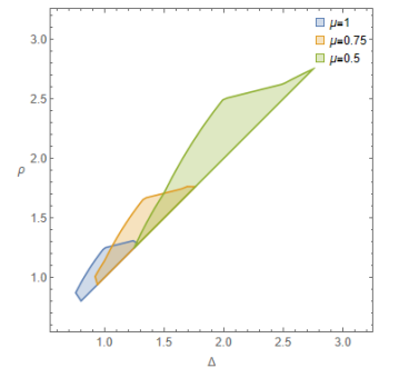
  Figure 2. Values of $\rho_{t}$ and $\Delta_{t}$, such that $\alpha_{t}<1$ for $\mu=1,0.75$ and $0.5$. For the smaller step sizes the range of acceptable parameters is bigger and also shifts to allow bigger distortion.

Now we are ready to proceed with the proof of Theorem 10, starting with the following key helper lemmas.

Lemma 3.

Let all quantities be as defined in the statement of Theorem 10, in particular, $\bm{A}{\bm{x}}^{*}={\bm{b}}$. For some ${\bm{x}}$ and ${\bm{y}}\in\mathbb{R}^{n^{d}}$, let $\rho>0$ be such that

(22) $$\|\bm{A}_{t}({\bm{x}}-{\bm{y}})\|_{2}^{2}\leq\rho\|{\bm{x}}-{\bm{y}}\|_{2}^{2}.$$

Then, for a function $f({\bm{z}}):=\|\bm{A}_{t}{\bm{z}}-{\bm{b}}\|_{2}^{2}/2$, it holds

(23) $$f({\bm{y}})\leq f({\bm{x}})+\left\langle\bm{A}_{t}^{T}\bm{A}_{t}\left({\bm{x}}-{\bm{x}}^{*}\right),{\bm{y}}-{\bm{x}}\right\rangle+\frac{\rho}{2}\|{\bm{y}}-{\bm{x}}\|_{2}^{2}.$$

Proof.

Let $\chi(s):={\bm{x}}+s({\bm{y}}-{\bm{x}})$ for $s\in[0,1]$. From the fundamental theorem of calculus, using that $\nabla f({\bm{z}})=\bm{A}_{t}^{T}\bm{A}_{t}({\bm{z}}-{\bm{x}}^{*})$, we have

$$f({\bm{y}})-f({\bm{x}})=\int_{0}^{1}(f\circ\chi)^{\prime}(s)ds =\int_{0}^{1}\nabla f(\chi(s))\chi^{\prime}(s)ds$$

$$=\int_{0}^{1}\left\langle\bm{A}_{t}^{T}\bm{A}_{t}\left({\bm{x}}+s({\bm{y}}-{\bm{x}})-{\bm{x}}^{*}\right),{\bm{y}}-{\bm{x}}\right\rangle ds$$

$$=\left\langle\bm{A}_{t}^{T}\bm{A}_{t}\left({\bm{x}}-{\bm{x}}^{*}\right),{\bm{y}}-{\bm{x}}\right\rangle+\int_{0}^{1}\left\langle s\bm{A}_{t}^{T}\bm{A}_{t}\left({\bm{y}}-{\bm{x}}\right),{\bm{y}}-{\bm{x}}\right\rangle ds$$

$$=\left\langle\bm{A}_{t}^{T}\bm{A}_{t}\left({\bm{x}}-{\bm{x}}^{*}\right),{\bm{y}}-{\bm{x}}\right\rangle+\frac{1}{2}\|\bm{A}_{t}({\bm{y}}-{\bm{x}})\|_{2}^{2}$$

$$\overset{\eqref{eq:lem3-cond}}{\leq}\left\langle\bm{A}_{t}^{T}\bm{A}_{t}\left({\bm{x}}-{\bm{x}}^{*}\right),{\bm{y}}-{\bm{x}}\right\rangle+\frac{\rho}{2}\|{\bm{y}}-{\bm{x}}\|_{2}^{2}.$$

This immediately gives (23). ∎

Lemma 4.

Let all quantities be as defined in the statement of Theorem 10. Then,

$$\|P_{\Omega_{t}}(\bm{A}_{t}^{T}\bm{A}_{t}{\bm{r}}^{t})\|_{F}^{2}\leq\rho_{t}\|\bm{A}_{t}{\bm{r}}^{t}\|_{F}^{2}\quad\text{ where }{\bm{r}}^{t}:=\textnormal{{Vec}}({\bm{\mathcal{R}}}^{t}).$$

Proof.

The definition of $\rho_{t}$ (19) impies that (22) holds with

$${\bm{x}}=\textnormal{{Vec}}({\bm{\mathcal{X}}}^{t})\text{ and }{\bm{y}}={\bm{x}}-\frac{1}{\rho_{t}}P_{\Omega_{t}}(\bm{A}_{t}^{T}\bm{A}_{t}{\bm{r}}^{t}).$$

We can apply Lemma 3 as follows:

$$f\big{(}{\bm{x}}- \frac{1}{\rho_{t}}P_{\Omega_{t}}(\bm{A}_{t}^{T}\bm{A}_{t}{\bm{r}}^{t})\big{)}$$

$$\leq f({\bm{x}})-\left\langle\bm{A}_{t}^{T}\bm{A}_{t}{\bm{r}}^{t},\frac{1}{\rho_{t}}P_{\Omega_{t}}(\bm{A}_{t}^{T}\bm{A}_{t}{\bm{r}}^{t})\right\rangle+\frac{\rho_{t}}{2}\left\|\frac{1}{\rho_{t}}P_{\Omega_{t}}(\bm{A}_{t}^{T}\bm{A}_{t}{\bm{r}}^{t})\right\|_{2}^{2}$$

$$\leq f({\bm{x}})-\left\langle P_{\Omega_{t}}(\bm{A}_{t}^{T}\bm{A}_{t}{\bm{r}}^{t}),\frac{1}{\rho_{t}}P_{\Omega_{t}}(\bm{A}_{t}^{T}\bm{A}_{t}{\bm{r}}^{t})\right\rangle+\frac{1}{2\rho_{t}}\left\|P_{\Omega_{t}}(\bm{A}_{t}^{T}\bm{A}_{t}{\bm{r}}^{t})\right\|_{2}^{2}$$

$$\leq\frac{1}{2}\|\bm{A}_{t}{\bm{r}}^{t}\|_{2}^{2}-\frac{1}{2\rho_{t}}\left\|P_{\Omega}(\bm{A}_{t}^{T}\bm{A}_{t}{\bm{r}}^{t})\right\|_{2}^{2},$$

where in the last step we observe that $f(\textnormal{{Vec}}({\bm{\mathcal{X}}}^{t}))=\frac{1}{2}\|\bm{A}_{t}{\bm{\mathcal{X}}}^{t}-\bm{A}_{t}{\bm{\mathcal{X}}}^{*}\|_{2}^{2}=\frac{1}{2}\|\bm{A}_{t}\textnormal{{Vec}}({\bm{\mathcal{R}}}^{t})\|^{2}$. Now, since $f(.)\geq 0$ we can conclude from above

$$\|P_{\Omega_{t}}(\bm{A}_{t}^{T}\bm{A}_{t}\textnormal{{Vec}}({\bm{\mathcal{R}}}^{t}))\|_{2}^{2}\leq\rho_{t}\|\bm{A}_{t}\textnormal{{Vec}}({\bm{\mathcal{R}}}^{t})\|_{2}^{2}.$$

∎

Proof of Theorem 10.

From the definition of $\xi_{t}$, we can conclude that for ${\bm{\mathcal{R}}}^{t+1}={\bm{\mathcal{X}}}^{t+1}-{\bm{\mathcal{X}}}^{*}$,

$$\|{\bm{\mathcal{R}}}^{t+1}+{\bm{\mathcal{X}}}^{*}-{\bm{\mathcal{Y}}}^{t}\|_{F}^{2}\leq(1+2\xi_{t}+\xi_{t}^{2})\|{\bm{\mathcal{Y}}}^{t}-{\bm{\mathcal{X}}}^{\ast}\|_{F}^{2},$$

and so

$$\|{\bm{\mathcal{R}}}^{t+1}\|_{F}^{2}\leq 2\underbrace{\langle{\bm{\mathcal{R}}}^{t+1},{\bm{\mathcal{Y}}}^{t}-{\bm{\mathcal{X}}}^{*}\rangle}_{\text{\tt{Term 1}}}+(2\xi_{t}+\xi_{t}^{2})\underbrace{\|{\bm{\mathcal{Y}}}^{t}-{\bm{\mathcal{X}}}^{\ast}\|_{F}^{2}}_{\text{\tt{Term 2}}}.$$

Bounding Term 1: Let $\Omega_{t}^{\prime}=span\{{\bm{\mathcal{R}}}^{t+1}\}\subseteq span\{\textnormal{{Vec}}({\bm{\mathcal{R}}}^{t}),\textnormal{{Vec}}({\bm{\mathcal{R}}}^{t+1})\}=\Omega_{t}$ and recall that $\textnormal{{Vec}}({\bm{\mathcal{Y}}}^{t}-{\bm{\mathcal{X}}}^{\ast})=(\bm{I}-\mu_{t}\bm{A}_{t}^{T}\bm{A}_{t}){\bm{r}}^{t}$, where ${\bm{r}}^{t}:=\textnormal{{Vec}}({\bm{\mathcal{R}}}^{t})$. We can bound

$$\langle{\bm{\mathcal{R}}}^{t+1},{\bm{\mathcal{Y}}}^{t}-{\bm{\mathcal{X}}}^{*}\rangle =\|{\bm{\mathcal{R}}}^{t+1}\|_{F}\|P_{\Omega^{\prime}_{t}}\left((\bm{I}-\mu_{t}\bm{A}_{t}^{T}\bm{A}_{t}){\bm{r}}^{t}\right)\|_{2}$$

$$\overset{\Omega^{\prime}_{t}\subseteq\Omega_{t}}{\leq}\|{\bm{\mathcal{R}}}^{t+1}\|_{F}\|P_{\Omega_{t}}\left((\bm{I}-\mu_{t}\bm{A}_{t}^{T}\bm{A}_{t}){\bm{r}}^{t}\right)\|_{2}$$

$$\overset{(a)}{\leq}\|{\bm{\mathcal{R}}}^{t+1}\|_{F}\sqrt{\|{\bm{r}}^{t}\|_{2}^{2}+\rho_{t}\mu_{t}^{2}\|\mathcal{A}_{t}({\bm{\mathcal{R}}}^{t})\|_{2}^{2}-2\mu_{t}\langle{\bm{r}}^{t},P_{\Omega_{t}}(\bm{A}_{t}^{T}\bm{A}_{t}{\bm{r}}^{t})\rangle}$$

$$\leq\|{\bm{\mathcal{R}}}^{t+1}\|_{F}\sqrt{\|{\bm{r}}^{t}\|_{2}^{2}+\rho_{t}\mu_{t}^{2}\|\bm{A}_{t}{\bm{r}}^{t}\|_{2}^{2}-2\mu_{t}\|\bm{A}_{t}{\bm{r}}^{t}\|_{2}^{2}}$$

$$\overset{(b)}{\leq}\|{\bm{\mathcal{R}}}^{t+1}\|_{F}\sqrt{\|{\bm{\mathcal{R}}}^{t}\|_{F}^{2}\left(1-(2-\mu_{t}\rho_{t})\mu_{t}\Delta_{t}\right)}.$$

Here, inequality $(a)$ follows from Lemma 4 and $(b)$ follows from the definition of $\Delta_{t}$ in (18).

Bounding Term 2:

$$\|\textnormal{{Vec}}({\bm{\mathcal{Y}}}^{t}-{\bm{\mathcal{X}}}^{\ast})\|_{2} \leq\|{\bm{\mathcal{R}}}^{t}\|_{F}+\mu_{t}\|\bm{A}_{t}^{T}\bm{A}_{t}\textnormal{{Vec}}({\bm{\mathcal{R}}}^{t})\|_{2}$$

$$\leq\|{\bm{\mathcal{R}}}^{t}\|_{F}+\mu_{t}\|\bm{A}_{t}\|_{2}\|\bm{A}_{t}({\bm{\mathcal{R}}}^{t})\|_{2}$$

$$=\left(1+\mu_{t}\|\bm{A}_{t}\|_{2}\sqrt{\Delta_{t}}\right)\|{\bm{\mathcal{R}}}^{t}\|_{F}\;.$$

Combining it all, we get that

$$\|{\bm{\mathcal{R}}}^{t+1}\|_{F}^{2}\leq 2\sqrt{1-(2-\mu_{t}\rho_{t})\mu_{t}\Delta_{t}}\|{\bm{\mathcal{R}}}^{t+1}\|_{F}\|{\bm{\mathcal{R}}}^{t}\|_{F}+\left(1+\|\bm{A}_{t}\|_{2}\mu_{t}\sqrt{\Delta_{t}}\right)^{2}\|{\bm{\mathcal{R}}}^{t}\|_{F}^{2}.$$

This implies that there exists $0\leq\alpha\leq 1$ such that

$$(1-\alpha)\|{\bm{\mathcal{R}}}^{t+1}\|_{F}^{2}\leq 2\sqrt{1-(2-\mu_{t}\rho_{t})\mu_{t}\Delta_{t}}\|{\bm{\mathcal{R}}}^{t+1}\|\|{\bm{\mathcal{R}}}^{t}\|_{F}\;.$$

$$\alpha\|{\bm{\mathcal{R}}}^{t+1}\|_{F}^{2}\leq(2\xi_{t}+\xi_{t}^{2})\left(1+\|\bm{A}_{t}\|_{2}\mu_{t}\sqrt{\Delta_{t}}\right)^{2}\|{\bm{\mathcal{R}}}^{t}\|_{F}^{2}\;.$$

Combining these gives us,

$$\left(1-\alpha+\sqrt{\alpha}\right)\|{\bm{\mathcal{R}}}^{t+1}\|_{F} \leq\left(2\sqrt{1-(2-\mu_{t}\rho_{t})\mu_{t}\Delta_{t}}+\sqrt{2\xi_{t}+\xi_{t}^{2}}\left(1+\mu_{t}\|\bm{A}_{t}\|_{2}\sqrt{1+\delta_{t}}\right)\right)\|{\bm{\mathcal{R}}}^{t}\|_{F}\;.$$

However, the function $(1-\alpha+\sqrt{\alpha})\geq 1$ on the interval $[0,1]$. So,

$$\|{\bm{\mathcal{R}}}^{t+1}\|_{F}\leq\left(2\sqrt{1-(2-\mu_{t}\rho_{t})\mu_{t}\Delta_{t}}+\sqrt{(2\xi_{t}+\xi_{t}^{2})}\left(1+\mu_{t}\|\bm{A}_{t}\|_{2}\sqrt{\Delta_{t}}\right)\right)\|{\bm{\mathcal{R}}}^{t}\|_{F},$$

which concludes the proof of Theorem 10. ∎

Remark 6.

Lemma 4 also implies that $\rho_{t}\geq\Delta_{t}$ for any $t\geq 1$. Indeed, note that the norm of the projection of $\bm{A}_{t}^{T}\bm{A}_{t}{\bm{r}}^{t}$ onto $\Omega=span\{{\bm{r}}^{t},{\bm{r}}^{t+1}\}$ is not smaller than the norm of its projection onto the subspace $\Omega^{\prime}=span\{{\bm{r}}^{t}\}$. Thus,

$$\rho_{t}\|\bm{A}_{t}{\bm{r}}^{t}\|_{2}^{2} \geq\|P_{\Omega}(\bm{A}_{t}^{T}\bm{A}_{t}{\bm{r}}^{t})\|_{2}^{2}\geq\|P_{\Omega^{\prime}}(\bm{A}_{t}^{T}\bm{A}_{t}{\bm{r}}^{t})\|_{2}^{2}$$

$$\geq\left\|\langle{\bm{r}}^{t},\bm{A}_{t}^{T}\bm{A}_{t}{\bm{r}}^{t}\rangle\frac{{\bm{r}}^{t}}{\|{\bm{r}}^{t}\|_{2}^{2}}\right\|_{2}^{2}\geq\frac{\|\bm{A}_{t}{\bm{r}}^{t}\|_{2}^{4}}{\|{\bm{r}}^{t}\|_{2}^{2}}\;.$$

This gives $\rho_{t}\|{\bm{\mathcal{R}}}^{t}\|_{2}^{2}\geq\|\bm{A}_{t}\textnormal{{Vec}}({\bm{\mathcal{R}}}^{t})\|_{2}^{2}=\Delta_{t}\|{\bm{\mathcal{R}}}^{t}\|_{F}^{2}$.

4.3. Analysis of KaczTIHT

Next, we give the convergence result for KaczTIHT. In Theorem 11 below, we show that the algorithm has exponential convergence rate given good Gaussian-like measurements and efficient tensor low-rank fitting sub-routine. We formalize these assumptions as follows:

Assumption 1: (Distribution) Let the matrix $\bm{A}\in\mathbb{R}^{m\times n^{d}}$ of a linear measurement operator $\mathcal{A}:\mathbb{R}^{n\times n\dots\times n}\rightarrow\mathbb{R}^{m}$ satisfy the following properties: its rows $\{{\bm{a}}_{i}\}_{i\in[m]}\subset\mathbbm{S}^{n^{d}-1}(0,\sqrt{n^{d}})$ are random vectors sampled independently from a mean zero, isotropic sub-Gaussian distribution with a sub-Gaussian norm $\ell$.

We assume that all the modes have the same directon for the simplicity of exposition. Note that while we can always properly rescale the rows of $\bm{A}$, the sub-Gaussian assumptions are quite strong. As a result, our subsequent theoretical guarantees include classes of standard RIP-measurements, such as, rescaled Gaussian measurements. Actually, even stronger results can be similarly concluded for bounded orthogonal measurement ensembles, such as those based on randomly subsampled descrete Fourier or Hadamard transforms — similarly to the vector case in [60] – see Remark 7 below. However, explaining the empirically observed advantage of KaczTIHT over TIHT, especially on non-RIP measurements such as tensor-structured measurements as considered above, should be a very interesting avenue for the future work.

Again, a good low-rank fitting routine is essential for the successful thresholding step:

Assumption 2: Assume that the thresholding operation $T_{\bm{r}}$ used in Algorithm 2 is such that

(24) $$\|{\bm{\mathcal{U}}}^{k}-{\bm{\mathcal{X}}}_{1}^{k+1}\|^{2}_{F}\leq(1+\xi)^{2}\|{\bm{\mathcal{U}}}^{k}-{\bm{\mathcal{X}}}^{\ast}\|_{F}^{2}\;,\\$$

for

$$\xi=\frac{\delta^{2}}{5\left(1+\delta+\left\|\frac{1}{\sqrt{m}}\bm{A}\right\|_{2}\sqrt{1+\delta}\right)^{2}}\;.$$

Note that, if we use the algorithm described in Theorem 3 with $\varepsilon=\xi$, then (24) automatically holds for the thresholding sub-routine in KaczTIHT 2. The same is true for the low rank CP thresholding using Theorem 2 for a suitably chosen $\varepsilon$ under mild assumptions.

Theorem 11 (Analysis of KaczTIHT).

Consider a tensor ${\bm{\mathcal{X}}}^{\ast}\in\mathbb{R}^{n\times n\dots\times n}$ of HOSVD rank ${\bm{r}}=(r,r,\dots,r)$ (or CP rank $r$). Let ${\bm{\mathcal{R}}}^{t}={\bm{\mathcal{X}}}_{1}^{t}-{\bm{\mathcal{X}}}^{\ast}$ be the residuals of the KaczTIHT Algorithm 2 applied to the linear measurements ${\bm{b}}=\mathcal{A}({\bm{\mathcal{X}}}^{\ast})+\bm{\eta}$, where $\bm{\eta}\geq 0$ is the measurement noise and $\mathcal{A}:\mathbb{R}^{n\times n\dots\times n}\rightarrow\mathbb{R}^{m}$ is a linear measurement operator satisfying Assumption 1. Assume that for some $\delta\in\left(0,\frac{1}{5}\right)$, the step-sizes $\gamma,\lambda>0$ in Algorithm 2 are taken to be

(25) $$\gamma\leq\frac{\delta}{2\sqrt{n^{d}}m\ell^{2}\ln^{2}m},\quad\lambda=\frac{n^{d}}{m\gamma}\;,$$

and Assumption 2 on the thresholding operator holds.

Then, as long as

$$m\geq C^{\prime}\delta^{-2}((3r)^{d}+9nrd)\ln(d)\ln^{2}(m)\ \text{for HOSVD rank ${\bm{r}}$ or }$$

$$m\geq C^{\prime}\delta^{-2}((3r)^{d}+3nrd)\ln(d)\ln^{2}(m)\ \text{for CP rank-$r$, }$$

with high probability $1-(m^{2}+1)e^{-C\ln^{2}m}$, we have

$$\|{\bm{\mathcal{R}}}^{k+1}\|_{F}\leq(5\delta)^{k+1}\|{\bm{\mathcal{R}}}^{0}\|_{F}+\frac{1}{m}\frac{\delta+2}{1-5\delta}\left(\left(\frac{\delta}{2(\ell\ln m)^{2}}+\frac{\delta^{2}}{2n^{d}(\ell\ln m)^{2}}\right)\|\bm{\eta}\|_{1}+\|\bm{A}^{\intercal}\bm{\eta}\|_{2}\right).$$

Here, $C,C^{\prime}>0$ are absolute constants that depends on the sub-Gaussian norm $l$, $\bm{A}$ is the matrix for of the measurement operator $\mathcal{A}$.

Before proceeding to the proof of Theorem 11, let’s take a closer look at the updates performed by inner relaxed Kaczmarz loop in the KaczTIHT Algorithm 2 algorithm. The next lemma is the result of a technical rewriting of Step 4 of the algorithm, essentially the same as in the vector case in [60, Lemma 1]:

Lemma 5.

In the notations of Theorem 11, the iterates $\{{\bm{\mathcal{X}}}_{i}^{j}\}$ of KaczTIHT satisfy

$$\textnormal{{Vec}}({\bm{\mathcal{X}}}_{m+1}^{k}-{\bm{\mathcal{X}}}^{\ast})=\left(\bm{I}-\frac{\gamma}{n^{d}}\bm{A}^{\intercal}\bm{A}+\bm{B}_{\tau}\right)\textnormal{{Vec}}({\bm{\mathcal{X}}}_{1}^{k}-{\bm{\mathcal{X}}}^{\ast})+\bm{\eta}_{err}.$$

where, if we denote ${\bm{a}}_{i}$ for $i=1,\ldots,m$ the rows of $\bm{A}$, and $\tau(i)$ is the permutation that we chosen for the $k$-th epoch, $\bm{B}_{\tau}:=\bm{B}_{\tau(m)}$, and

(26) $$\bm{B}_{\tau(k)}:=\frac{\gamma^{2}}{n^{2d}} \sum_{m-k+1\leq i_{1}<i_{2}\leq m}{\bm{a}}_{\tau(i_{2})}{\bm{a}}_{\tau(i_{2})}^{\intercal}{\bm{a}}_{\tau(i_{1})}{\bm{a}}_{\tau(i_{1})}^{\intercal}$$

$$-\frac{\gamma^{3}}{n^{3d}}\sum_{m-k+1\leq i_{1}<i_{2}<i_{3}\leq m}{\bm{a}}_{\tau(i_{3})}{\bm{a}}_{\tau(i_{3})}^{\intercal}{\bm{a}}_{\tau(i_{2})}{\bm{a}}_{\tau(i_{2})}^{\intercal}{\bm{a}}_{\tau(i_{1})}{\bm{a}}_{\tau(i_{1})}^{\intercal}+\dots,$$

and

$$\bm{\eta}_{err}:=\frac{\gamma}{n^{d}}\sum_{i=0}^{m-1}\bm{\eta}_{\tau(m-i)}\left(\bm{I}-\sum_{j=m-i+1}^{m}\frac{\gamma}{n^{d}}{\bm{a}}_{\tau(j)}{\bm{a}}_{\tau(j)}^{\intercal}+\bm{B}_{\tau(i)}\right){\bm{a}}_{\tau(m-i)}.$$

Proof.

Straightforward check, starting with

$$\textnormal{{Vec}}({\bm{\mathcal{X}}}_{m+1}^{k}-{\bm{\mathcal{X}}}^{\ast})= \left(\prod_{i=1}^{m}(\bm{I}-\frac{\gamma}{n^{d}}{{\bm{a}}_{\tau(i)}{\bm{a}}_{\tau(i)}^{\intercal}})\right)\textnormal{{Vec}}({\bm{\mathcal{X}}}_{1}^{k}-{\bm{\mathcal{X}}}^{\ast})$$

$$+{\gamma\sum_{i=0}^{m-1}\frac{\bm{\eta}_{\tau(m-i)}}{n^{d}}{\bm{a}}_{\tau(m-i)}\prod_{j=0}^{i-1}\left(\bm{I}-\frac{\gamma}{n^{d}}{{\bm{a}}_{\tau(m-j)}{\bm{a}}^{\intercal}_{\tau(m-j)}}\right)}\;.$$

∎

We need two more technical lemmas bounding the quantities involved:

Lemma 6 (Bounding $\bm{B}_{\tau(k)}$).

Given a measurement operator $\mathcal{A}:\mathbb{R}^{n\times n\times\dots\times n}\rightarrow\mathbb{R}^{m}$ and $\bm{B}_{\tau(k)}$ for any $k\in[m]$ defined as above (26) and $0<\delta<1$, we have that for for any $k\in[m]$,

$$\lambda\|\bm{B}_{\tau(k)}\|_{2}\leq\delta,$$

with probability at least $1-m^{2}e^{-C\ln^{2}(m)}$ where $\lambda$ is as in (25).

Proof.

We have that

$$\|{\bm{a}}_{\tau(i_{2})}{\bm{a}}_{\tau(i_{2})}^{\intercal}{\bm{a}}_{\tau(i_{1})}{\bm{a}}_{\tau(i_{1})}^{\intercal}\|_{2}\leq\|{\bm{a}}_{\tau(i_{2})}\|_{2}\|{\bm{a}}_{\tau(i_{1})}\|_{2}|\langle{\bm{a}}_{\tau(i_{2})},{\bm{a}}_{\tau(i_{1})}\rangle|\leq n^{d}|\langle{\bm{a}}_{\tau(i_{2})},{\bm{a}}_{\tau(i_{1})}\rangle|\;,$$

and,

$$\|{\bm{a}}_{\tau(i_{p})}{\bm{a}}_{\tau(i_{p})}^{\intercal}\dots\bm{a}_{\tau(i_{1})}{\bm{a}}_{\tau(i_{1})}^{\intercal}\|_{2} \leq\|{\bm{a}}_{\tau(i_{p})}\|_{2}\|{\bm{a}}_{\tau(i_{1})}\|_{2}|\langle{\bm{a}}_{\tau(i_{p})},{\bm{a}}_{\tau(i_{p-1})}\rangle|\dots|\langle{\bm{a}}_{\tau(i_{2})},{\bm{a}}_{\tau(i_{1})}\rangle|$$

(27) $$\leq n^{d}|\langle{\bm{a}}_{\tau(i_{p})},{\bm{a}}_{\tau(i_{p-1})}\rangle|\dots|\langle{\bm{a}}_{\tau(i_{2})},{\bm{a}}_{\tau(i_{1})}\rangle|\;.$$

Further, it follows from Lemma 1 with $t=\ln(m)$ via a union bound argument that for any $i\neq j\in[m]$, with probability at least $1-m^{2}e^{-C\ln^{2}(m)}$,

$$|\langle{\bm{a}}_{i},{\bm{a}}_{j}\rangle|\leq\ell^{2}\sqrt{n^{d}}\ln^{2}m.$$

Here, $C$ is a positive absolute constant. Then,

$$\left\|\frac{\gamma^{p}}{n^{dp}}\sum_{m-k+1\leq i_{1}<i_{2}\dots i_{p}\leq m}{\bm{a}}_{\tau(i_{p})}{\bm{a}}_{\tau(i_{p})}^{\intercal}\dots\bm{a}_{\tau(i_{2})}{\bm{a}}_{\tau(i_{2})}^{\intercal}{\bm{a}}_{\tau(i_{1})}{\bm{a}}_{\tau(i_{1})}^{\intercal}\right\|_{2} \leq\frac{\gamma^{p}}{n^{dp}}\binom{m}{p}n^{d}(\ell^{4}n^{d}\ln^{4}(m))^{\frac{p-1}{2}}$$

$$\leq(\gamma m)^{p}\left({\ell^{4}\ln^{4}(m)}{n^{-d}}\right)^{\frac{p-1}{2}}\;.$$

Thus, for any $k\in[m]$,

$$\|\bm{B}_{\tau(k)}\|_{2}\leq\sum_{p=2}^{m}(\gamma m)^{p}\left({\ell^{4}\ln^{4}(m)}{n^{-d}}\right)^{\frac{p-1}{2}}\leq 2\gamma^{2}m^{2}\ell^{2}\ln^{2}(m)n^{-d/2}.$$

Using (25), we can conclude that $\lambda\|\bm{B}_{\tau(k)}\|_{2}\leq\delta$.

∎

Lemma 7.

Given a measurement operator $\mathcal{A}:\mathbb{R}^{n\times n\times\dots\times n}\rightarrow\mathbb{R}^{m}$ that satisfies $(\delta,3{\bm{r}})$-TensorRIP, and HOSVD rank ${\bm{r}}$ (or, CP rank $r$) tensors ${\bm{\mathcal{X}}}$, ${\bm{\mathcal{Y}}}$ and ${\bm{\mathcal{Z}}}\in\mathbb{R}^{n\times n\times\dots\times n}$, we have that

$$\left|\big{\langle}\left(\bm{I}-\bm{A}^{\intercal}\bm{A}\right)\textnormal{{Vec}}({\bm{\mathcal{X}}}-{\bm{\mathcal{Z}}}),\textnormal{{Vec}}({\bm{\mathcal{Y}}}-{\bm{\mathcal{Z}}})\big{\rangle}\right|\leq\delta\|{\bm{\mathcal{X}}}-{\bm{\mathcal{Z}}}\|_{F}\|{\bm{\mathcal{Y}}}-{\bm{\mathcal{Z}}}\|_{F},$$

where $\bm{A}\in\mathbb{R}^{m\times n^{d}}$ corresponds to the operator $\mathcal{A}$.

Proof.

Without loss of generality, we can assume that ${\bm{\mathcal{Z}}}_{1}:={\bm{\mathcal{X}}}-{\bm{\mathcal{Z}}}$ and ${\bm{\mathcal{Z}}}_{2}:={\bm{\mathcal{Y}}}-{\bm{\mathcal{Z}}}$ are unit norm tensors, let ${\bm{z}}_{1}=\textnormal{{Vec}}({\bm{\mathcal{Z}}}_{1})$ and ${\bm{z}}_{2}=\textnormal{{Vec}}({\bm{\mathcal{Z}}}_{2})$. By the parallelogram law,

$$\big{|}\left\langle\bm{A}{\bm{z}}_{1},\bm{A}{\bm{z}}_{2}\right\rangle-\left\langle{\bm{z}}_{1},{\bm{z}}_{2}\right\rangle\big{|}\leq\frac{1}{4}\big{|}\|\bm{A}({\bm{z}}_{1}+{\bm{z}}_{2})\|^{2}-\|\bm{A}({\bm{z}}_{1}-{\bm{z}}_{2})\|^{2}-\|{\bm{z}}_{1}+{\bm{z}}_{2}\|^{2}+\|{\bm{z}}_{1}-{\bm{z}}_{2}\|^{2}\big{|}.$$

Now note that, ${\bm{\mathcal{Z}}}_{1}\pm{\bm{\mathcal{Z}}}_{2}$ are HOSVD rank $3{\bm{r}}$ (or equivalently CP rank $3r$) tensors. By using the fact that $\bm{A}$ satisfies $(\delta,3{\bm{r}})$-TensorRIP we have

$$\big{|}\left\langle\bm{A}{\bm{z}}_{1},\bm{A}{\bm{z}}_{2}\right\rangle-\left\langle{\bm{z}}_{1},{\bm{z}}_{2}\right\rangle\big{|}\leq\frac{\delta}{4}\left(\|{\bm{\mathcal{Z}}}_{1}+{\bm{\mathcal{Z}}}_{2}\|_{F}^{2}+\|{\bm{\mathcal{Z}}}_{1}-{\bm{\mathcal{Z}}}_{2}\|_{F}^{2}\right)\leq\delta,$$

applying the parallelogram law and the unit norm assumption in the last step. Rearranging, this concludes the proof of the lemma. ∎

With these results in place, we can proceed to prove the main theorem.

Proof of Theorem 11.

From Assumption 2, we know that,

$$\|{\bm{\mathcal{U}}}^{k}-{\bm{\mathcal{X}}}_{1}^{k+1}\|^{2}_{F}=\|({\bm{\mathcal{U}}}^{k}-{\bm{\mathcal{X}}}^{\ast})+({\bm{\mathcal{X}}}^{\ast}-{\bm{\mathcal{X}}}_{1}^{k+1})\|^{2}_{F}\leq(1+\xi)^{2}\|{\bm{\mathcal{U}}}^{k}-{\bm{\mathcal{X}}}^{\ast}\|_{F}^{2}\;.$$

which implies

$$\|{\bm{\mathcal{X}}}^{\ast}-{\bm{\mathcal{X}}}_{1}^{k+1}\|_{F}^{2}\leq 2\underbrace{\langle{\bm{\mathcal{U}}}^{k}-{\bm{\mathcal{X}}}^{\ast},{\bm{\mathcal{X}}}_{1}^{k+1}-{\bm{\mathcal{X}}}^{\ast}\rangle}_{\text{\tt{Term 1}}}+\ (2\xi+\xi^{2})\underbrace{\|{\bm{\mathcal{U}}}^{k}-{\bm{\mathcal{X}}}^{\ast}\|_{F}^{2}}_{\text{\tt{Term 2}}}\;.$$

From Lemma 5, we know that

$$\textnormal{{Vec}}({\bm{\mathcal{X}}}_{m+1}^{k}-{\bm{\mathcal{X}}}_{1}^{k})=\left(-\frac{\gamma}{n^{d}}\bm{A}^{\intercal}\bm{A}+\bm{B}_{\tau}\right)\textnormal{{Vec}}({\bm{\mathcal{X}}}_{1}^{k}-{\bm{\mathcal{X}}}^{\ast})+\bm{\eta}_{err}.$$

Also, ${\bm{\mathcal{U}}}^{k}={\bm{\mathcal{X}}}_{1}^{k}+\lambda({\bm{\mathcal{X}}}_{m+1}^{k}-{\bm{\mathcal{X}}}_{1}^{k})$, giving us

$${\bm{\mathcal{U}}}_{k}-{\bm{\mathcal{X}}}^{*}=\left(\bm{I}-\lambda\frac{\gamma}{n^{d}}\bm{A}^{\intercal}\bm{A}+\lambda\bm{B}_{\tau}\right)({\bm{\mathcal{X}}}_{1}^{k}-{\bm{\mathcal{X}}}^{\ast})$$

By using Theorem 5 (or equivalently Theorem 6), we get that under our hypothesis, the measurement operator $\frac{1}{\sqrt{m}}\bm{A}$ also satisfies $(\delta,3{\bm{r}})$-TensorRIP (or equivalently $(\delta,3r)$-TensorRIP for low rank CP recovery) with probability at least $1-e^{-C\ln^{2}m}$ for some $C>0$. Together with Lemma 6, we get that with probability at least $1-(m^{2}+1)e^{-C\ln^{2}m}$

$$\|{\bm{\mathcal{U}}}^{k}-{\bm{\mathcal{X}}}^{\ast}\|_{F}=\left\|\left(\bm{I}-\frac{1}{m}{\bm{A}}^{\intercal}\bm{A}+\lambda\bm{B}_{\tau}\right)\textnormal{{Vec}}({\bm{\mathcal{X}}}_{1}^{k}-{\bm{\mathcal{X}}}^{\ast})+\lambda\bm{\eta}_{err}\right\|_{2}\quad(\text{Since }\lambda=\frac{n^{d}}{m\gamma})$$

$$\leq\|{\bm{\mathcal{X}}}_{1}^{k}-{\bm{\mathcal{X}}}^{\ast}\|_{F}+\left\|\frac{1}{\sqrt{m}}{\bm{A}}^{\intercal}\right\|_{2}\left\|\frac{1}{\sqrt{m}}\bm{A}\textnormal{{Vec}}({\bm{\mathcal{X}}}_{1}^{k}-{\bm{\mathcal{X}}}^{\ast})\right\|_{2}+\|\lambda\bm{B}_{\tau}\|_{2}\|{\bm{\mathcal{X}}}_{1}^{k}-{\bm{\mathcal{X}}}^{\ast}\|_{F}+\|\lambda\bm{\eta}_{err}\|_{2}$$

$$\leq\left(1+\delta+\left\|\frac{1}{\sqrt{m}}\bm{A}\right\|_{2}\sqrt{1+\delta}\right)\|{\bm{\mathcal{X}}}_{1}^{k}-{\bm{\mathcal{X}}}^{\ast}\|_{F}+\|\lambda\bm{\eta}_{err}\|_{2}\;.\quad(\text{Using \lx@cref{creftype~refnum}{lem:TRIP_and_bound_B_tau}})$$

and

$$\text{\tt{Term 2}}=\|{\bm{\mathcal{U}}}^{k}-{\bm{\mathcal{X}}}^{\ast}\|_{F}^{2}\leq 2\left(1+\delta+\left\|\frac{1}{\sqrt{m}}\bm{A}\right\|_{2}\sqrt{1+\delta}\right)^{2}\|{\bm{\mathcal{X}}}_{1}^{k}-{\bm{\mathcal{X}}}^{\ast}\|_{F}^{2}+2\|\lambda\bm{\eta}_{err}\|_{2}^{2};.$$

And, for Term 1 we get that, using Lemma 7,

$$\langle{\bm{\mathcal{U}}}^{k}-{\bm{\mathcal{X}}}^{\ast},{\bm{\mathcal{X}}}_{1}^{k+1}-{\bm{\mathcal{X}}}^{\ast}\rangle$$

$$=\left\langle\left(\bm{I}-\frac{1}{m}\bm{A}^{\intercal}\bm{A}\right)\textnormal{{Vec}}({\bm{\mathcal{X}}}_{1}^{k+1}-{\bm{\mathcal{X}}}^{\ast}),\textnormal{{Vec}}({\bm{\mathcal{X}}}_{1}^{k}-{\bm{\mathcal{X}}}^{\ast})\right\rangle$$

$$\quad\quad\quad\quad+\left\langle\lambda\bm{B}_{\tau}\textnormal{{Vec}}({\bm{\mathcal{X}}}_{1}^{k+1}-{\bm{\mathcal{X}}}^{\ast}),\textnormal{{Vec}}({\bm{\mathcal{X}}}_{1}^{k}-{\bm{\mathcal{X}}}^{\ast})\right\rangle+\left\langle\lambda\bm{\eta}_{err},\textnormal{{Vec}}({\bm{\mathcal{X}}}_{1}^{k+1}-{\bm{\mathcal{X}}}^{\ast})\right\rangle$$

$$\leq\delta\|{\bm{\mathcal{X}}}_{1}^{k+1}-{\bm{\mathcal{X}}}^{\ast}\|_{F}\|{\bm{\mathcal{X}}}_{1}^{k}-{\bm{\mathcal{X}}}^{\ast}\|_{F}+\|\lambda\bm{B}_{\tau}\|_{2}\|{\bm{\mathcal{X}}}_{1}^{k+1}-{\bm{\mathcal{X}}}^{\ast}\|_{F}\|{\bm{\mathcal{X}}}_{1}^{k}-{\bm{\mathcal{X}}}^{\ast}\|_{F}+\|\lambda\bm{\eta}_{err}\|_{2}\|{\bm{\mathcal{X}}}_{1}^{k+1}-{\bm{\mathcal{X}}}^{\ast}\|_{F}.$$

Putting this all together with Lemma 6, we get

$$\|{\bm{\mathcal{X}}}^{\ast}-{\bm{\mathcal{X}}}_{1}^{k+1}\|_{F}^{2} \leq 2(2\xi+\xi^{2})\left(\left(1+\delta+\left\|\frac{1}{\sqrt{m}}\bm{A}\right\|_{2}\sqrt{1+\delta}\right)^{2}\|{\bm{\mathcal{X}}}_{1}^{k}-{\bm{\mathcal{X}}}^{\ast}\|_{F}^{2}+\|\lambda\bm{\eta}_{err}\|_{2}^{2}\right)$$

$$\quad\quad\quad\quad+4\delta\|{\bm{\mathcal{X}}}_{1}^{k+1}-{\bm{\mathcal{X}}}^{\ast}\|_{F}\|{\bm{\mathcal{X}}}_{1}^{k}-{\bm{\mathcal{X}}}^{\ast}\|_{F}+2\|\lambda\bm{\eta}_{err}\|_{2}\|{\bm{\mathcal{X}}}_{1}^{k+1}-{\bm{\mathcal{X}}}^{\ast}\|_{F}.$$

This implies that there exist $\alpha,\beta,\pi\in[0,1]$ such that

$$(1-\alpha-\beta-\pi)\|{\bm{\mathcal{X}}}_{1}^{k+1}-{\bm{\mathcal{X}}}^{\ast}\|_{F}^{2}\leq 4\delta\|{\bm{\mathcal{X}}}_{1}^{k+1}-{\bm{\mathcal{X}}}^{\ast}\|_{F}\|{\bm{\mathcal{X}}}_{1}^{k}-{\bm{\mathcal{X}}}\|_{F}\;,$$

$$\alpha\|{\bm{\mathcal{X}}}_{1}^{k+1}-{\bm{\mathcal{X}}}^{\ast}\|_{F}^{2}\leq{2}(2\xi+\xi^{2})\left(1+\delta+\left\|\frac{1}{\sqrt{m}}\bm{A}\right\|_{2}\sqrt{1+\delta}\right)^{2}\|{\bm{\mathcal{X}}}^{k}_{1}-{\bm{\mathcal{X}}}^{\ast}\|_{F}^{2}\;,$$

$$\beta\|{\bm{\mathcal{X}}}_{1}^{k+1}-{\bm{\mathcal{X}}}^{\ast}\|_{F}^{2}\leq{2}(2\xi+\xi^{2})\|\lambda\bm{\eta}_{err}\|_{2}^{2}\;,$$

$$\pi\|{\bm{\mathcal{X}}}_{1}^{k+1}-{\bm{\mathcal{X}}}^{\ast}\|_{F}^{2}\leq 2\|\lambda\bm{\eta}_{err}\|_{2}\|{\bm{\mathcal{X}}}_{1}^{k+1}-{\bm{\mathcal{X}}}^{\ast}\|_{F}\;.$$

Then,

$$\|{\bm{\mathcal{X}}}_{1}^{k+1}-{\bm{\mathcal{X}}}^{\ast}\|_{F}\leq \ \frac{1}{{1-\alpha-\beta+\sqrt{\alpha}+\sqrt{\beta}}}\left[4\delta+\sqrt{4\xi+2\xi^{2}}\left(1+\delta+\left\|\frac{1}{\sqrt{m}}\bm{A}\right\|_{2}\sqrt{1+\delta}\right)\right]\|{\bm{\mathcal{X}}}^{k}_{1}-{\bm{\mathcal{X}}}^{\ast}\|_{2}$$

$$+\frac{\sqrt{4\xi+2\xi^{2}}+2}{{1-\alpha-\beta+\sqrt{\alpha}+\sqrt{\beta}}}\|\lambda\bm{\eta}_{err}\|_{2}\;.$$

Note that $\alpha,\beta\in[0,1]$ the function $(1-\alpha-\beta+\sqrt{\beta}+\sqrt{\alpha})^{-1}$ is positive and strictly bounded by $1$, also let $\sigma:=1+\delta+\|\frac{1}{\sqrt{m}}\bm{A}\|_{2}\sqrt{1+\delta}>1$. We know from (24), that the thresholding approximation is $\xi$-accurate where $\xi\leq\frac{\delta^{2}}{5\sigma^{2}}$. So, we have

$$\|{\bm{\mathcal{X}}}_{1}^{k+1}-{\bm{\mathcal{X}}}^{\ast}\|_{F} \leq(4\delta+\sigma\sqrt{4\xi+2\xi^{2}})\|{\bm{\mathcal{X}}}^{k}_{1}-{\bm{\mathcal{X}}}^{\ast}\|_{2}+(\sqrt{4\xi+2\xi^{2}}+2)\|\lambda\bm{\eta}_{err}\|_{2}$$

$$\leq 5\delta\|{\bm{\mathcal{X}}}_{1}^{k}-{\bm{\mathcal{X}}}^{\ast}\|_{F}+(\delta+2)\|\lambda\bm{\eta}_{err}\|_{2}$$

$$\leq(5\delta)^{k+1}\|{\bm{\mathcal{X}}}^{\ast}\|_{F}+\frac{\delta+2}{1-5\delta}\|\lambda\bm{\eta}_{err}\|_{2}.$$

Finally, we bound the $\bm{\eta}_{err}$ term as follows: from Lemma 5,

$$\|\lambda\bm{\eta_{err}}\|_{2} \leq\left\|\frac{1}{m}\sum_{i=0}^{m-1}\bm{\eta}_{\tau(m-i)}\left(\bm{I}-\sum_{j=m-i+1}^{m}\frac{\gamma}{n^{d}}{\bm{a}}_{\tau(j)}{\bm{a}}_{\tau(j)}^{\intercal}+\bm{B}_{\tau(i)}\right){\bm{a}}_{\tau(m-i)}\right\|_{2}$$

$$\leq\frac{1}{m}\left\|\sum_{i=1}^{m}\eta_{i}{\bm{a}}_{i}\right\|_{2}+\frac{\gamma}{n^{d}}\sum_{i=0}^{m-1}|\bm{\eta}_{\tau(m-i)}|\underset{j}{\max}\;\|{\bm{a}}_{\tau(j)}{\bm{a}}_{\tau(j)}^{\intercal}\|_{2}\underset{i}{\max}\|{\bm{a}}_{\tau(m-i)}\|_{2}$$

$$\quad\quad\quad\quad\quad\quad\quad\quad\quad\quad\quad+\frac{1}{m}\sum_{i=0}^{m-1}|\bm{\eta}_{\tau(m-i)}|\underset{i}{\max}\|\bm{B}_{\tau(i)}\|_{2}\|{\bm{a}}_{\tau(m-i)}\|_{2}$$

$$\leq\|\bm{A}^{\intercal}\bm{\eta\|_{2}}+\frac{1}{m}\left(\frac{\delta}{2(\ell\ln m)^{2}}+\frac{\delta^{2}}{2n^{d}(\ell\ln m)^{2}}\right)\|\bm{\eta}\|_{1}.$$

Finally we can conclude the proof with

$$\|{\bm{\mathcal{X}}}_{1}^{k+1}-{\bm{\mathcal{X}}}\|_{F}\leq(5\delta)^{k+1}\|{\bm{\mathcal{X}}}^{\ast}\|_{F}+\frac{1}{m}\frac{\delta+2}{1-5\delta}\left(\left(\frac{\delta}{2(\ell\ln m)^{2}}+\frac{\delta^{2}}{2n^{d}(\ell\ln m)^{2}}\right)\|\bm{\eta}\|_{1}+\|\bm{A}^{\intercal}\bm{\eta}\|_{2}\right).$$

∎

Remark 7 (KaczTIHT for BOS measurement matrix).

Note that when the measurement matrix $\bm{A}$, corresponding to the linear measurement operator $\mathcal{A}$, is sampled from a bounded orthogonal system, that is, the rows of $\bm{A}$ are orthogonal, KaczTIHT is equivalent to the standard TIHT iteration (similarly to the vector case in [60]). Indeed, we can simplify (5) to

$$\textnormal{{Vec}}\left({\bm{\mathcal{X}}}^{k}_{m+1}-{\bm{\mathcal{X}}}^{\ast}\right)=\left(\bm{I}-\gamma\sum_{i=1}^{m}\frac{{\bm{a}}_{\tau(i)}{\bm{a}}_{\tau(i)}^{\intercal}}{n^{d}}\right)\textnormal{{Vec}}({\bm{\mathcal{X}}}_{1}^{k}-{\bm{\mathcal{X}}}^{\ast})+\sum_{i=0}^{m-1}\bm{\eta}_{\tau(m-i)}\gamma\frac{{\bm{a}}_{\tau(m-i)}}{n^{d}}\;.$$

For the $\|{\bm{a}}_{j}\|^{2}=n^{d}$ for all $j=1,\dots m$ the step-sizes chosen to be $\gamma=n^{d}/m$ and $\lambda=1$,

$$\gamma\sum_{i=1}^{m}\frac{{\bm{a}}_{\tau(i)}{\bm{a}}_{\tau(i)}^{\intercal}}{\|{\bm{a}}_{\tau(i)}\|_{2}^{2}}=\frac{n}{m}\sum_{i=1}^{m}\frac{{\bm{a}}_{\tau(i)}{\bm{a}}_{\tau(i)}^{\intercal}}{n^{d}}=\frac{1}{m}\bm{A}^{\intercal}\bm{A}\;.$$

In this case, the iterates of KaczTIHT satisfy

$${\bm{\mathcal{X}}}_{m+1}^{k}={\bm{\mathcal{X}}}_{1}^{k}+\frac{1}{m}\bm{A}^{\intercal}\bm{A}\textnormal{{Vec}}({\bm{\mathcal{X}}}^{\ast}-{\bm{\mathcal{X}}}_{1}^{k})+\frac{1}{m}\bm{A}^{\intercal}\bm{\eta}={\bm{\mathcal{X}}}_{1}^{k}+\frac{1}{m}\bm{A}^{\intercal}({\bm{b}}-\bm{A}{\bm{\mathcal{X}}}_{1}^{k})),$$

$$\textnormal{{Vec}}({\bm{\mathcal{X}}}_{1}^{k+1})=T_{\mathbf{r}}(\textnormal{{Vec}}({\bm{\mathcal{X}}}^{k}_{m+1}))=T_{\mathbf{r}}\left({\bm{\mathcal{X}}}_{1}^{k}+\frac{1}{m}\bm{A}^{\intercal}({\bm{b}}-\bm{A}\textnormal{{Vec}}({\bm{\mathcal{X}}}_{1}^{k}))\right).$$

This coincides with the iterations of TIHT.

5. Experiments

The code can be found at https://github.com/shambhavi-suri/Low-Rank-Tensor-Recovery. All the experiments were run on Adroit, a Beowulf cluster, using 1 core with 20 GB RAM.

5.1. Synthetic Data

Numerical experiments comparing the performance of TIHT with the newly proposed algorithms KaczTIHT and TrimTIHT on synthetic data are presented here. We consider the recovery of low HOSVD and CP rank tensors which have been compressed using two different classes of measurement ensembles: entry-wise independent Gaussian $\mathcal{N}(0,1)$ measurements and face-splitting product of entry-wise independent Gaussian $\mathcal{N}(0,1)$ matrices. Relative error here corresponds to $\frac{\|{\bm{\mathcal{X}}}-{\bm{\mathcal{Y}}}\|_{F}}{{\|{\bm{\mathcal{X}}}\|_{F}}}$ where ${\bm{\mathcal{Y}}}$ is an estimate of ${\bm{\mathcal{X}}}$.

We restrict our attention to the tensors in $\mathbb{R}^{15\times 15\times 15}$. Low HOSVD rank ${\bm{r}}=(r,r,\dots,r)$ tensors are generated via a mode-wise product of a randomly sampled core tensor ${\bm{\mathcal{C}}}$ and orthogonal factor matrices $\bm{U}_{1},\bm{U}_{2}\ \text{and}\ \bm{U_{3}}$. More precisely, ${\bm{\mathcal{C}}}$ is generated by sampling entry-wise from a Gaussian $\mathcal{N}{(0,1)}+Unif(0,2)$ distribution and $\bm{U}_{i}$’s correspond to the top $r$ left singular vectors corresponding to a random matrix in $\mathbb{R}^{15\times 15}$ whose entries are sampled i.i.d from $\mathcal{N}{(0,1)}+Unif(0,2)$. Similarly, a random CP rank $r$ tensor is generated via random factors ${\bm{x}}_{ij}$ whose entries are sampled i.i.d from a random Gaussian $\mathcal{N}(0.1,1)$ distribution.

Choosing Parameters: For KaczTIHT, we set $\lambda=1$ and $\gamma=\frac{n^{d}}{m}$. While theory mandates a small choice of $\gamma$, we observe that empirically the performance did not depend on the values of these parameters as long as the product $\gamma\lambda=\frac{n^{d}}{m}$. For both TIHT and TrimTIHT, we consider the step-size $\mu=1$. This ensures a fair comparison, and enables us to study the effect of just trimming on the convergence rate. Further, for TrimTIHT, we select $m_{trim}$ by optimizing over a set of 5 values that range from 5 to 80, over 5 random sample runs.

5.1.1. Gaussian Measurements

In this experiment, we consider the compression of random low-rank tensors using entry-wise Gaussian $N(0,1)$ matrices. Gaussian matrices have good RIP properties and the standard low-rank recoverymethods are expected to work well. Yet, we demonstrate the advantage of the proposed adaptive methods that is especially prominent when the rank gets higher.

First, in Figure 3(A) and Figure 3(B), we consider the recovery of $50$ HOSVD rank $(2,2,2)$ and $(5,5,5)$ tensors respectively which have been compressed to different dimensions. We say that a tensor has been recovered, if the relative error is less than $10^{-4}$ after 200 iterations. We then record the fraction recovered at each compression level. TrimTIHT method performs the best for both these ranks and KaczTIHT outperforms vanilla TIHT at a higher rank, when TIHT recovery essentially fails. Similarly, the same experiment was repeated with CP rank $5$ tensors (Figure 3(C)), and here we observe that both KaczTIHT and TrimTIHT outperform TIHT with the former being more stable.

Subsequently in Figure 4, we compare the convergence of the considered IHT-based recovery methods, starting from a fixed number of measurements. We see that for both HOSVD and CP rank, KaczTIHT and TrimTIHT perform better than TIHT, and that KaczTIHT outperforms TrimTIHT as the rank increases.

5.1.2. Face-Splitting Measurements

Then, we consider the compression of random low-rank tensors using face-splitting product of entry-wise Gaussian $N(0,1)$ matrices. Such measurements do not have good RIP properties (recall Proposition 1) and empirically we see that the standard TIHT method does not recover the tensors from any compression ratio we considered (from up to $40\%$ of data). However, we show that the proposed methods enable the recovery.

In Figure 5(A) and Figure 5(B), we consider the recovery of $50$ HOSVD rank $(2,2,2)$ and $(5,5,5)$ tensors respectively which have been compressed to different dimensions. Similarly, the same experiment was repeated with CP rank $5$ tensors. Again, we say that the tensor has been recovered if the relative error is less than $10^{-4}$ after 200 iterations and record the fraction recovered at each compression level. Here, TIHT fails for all considered cases, whereas TrimTIHT and KaczTIHT are able to recover tensors from highly compressed measurements.

Then, in Figure 6, for a fixed number of measurements, we study the convergence of these methods. Again, we see that for both HOSVD and CP rank, KaczTIHT and TrimTIHT converge faster than TIHT. Additionally, KaczTIHT tends to perform better than TrimTIHT as the rank increases.

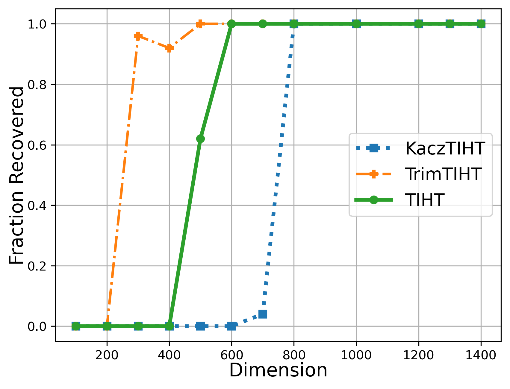
(a) HOSVD Rank$(2,2,2)$

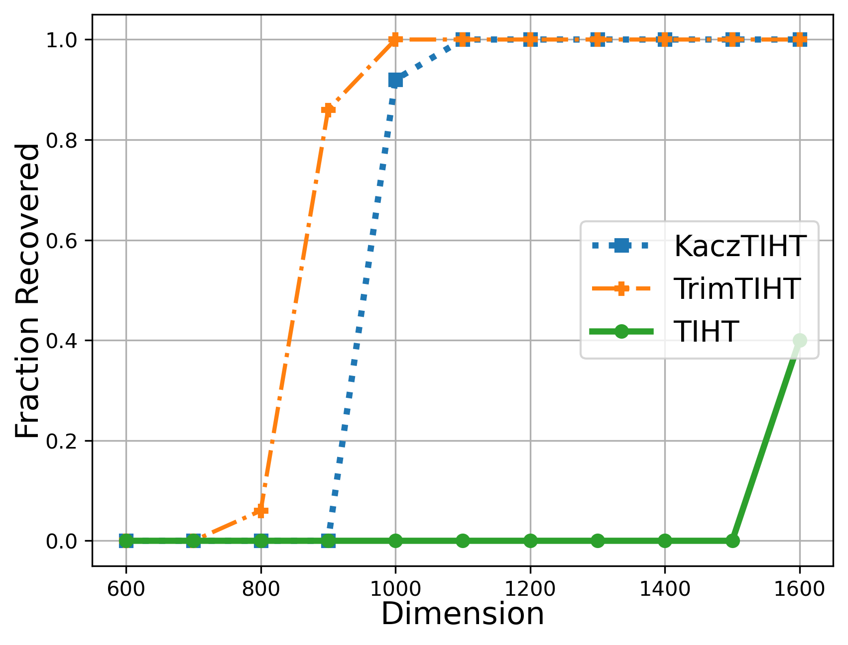
(b) HOSVD Rank $(5,5,5)$

(c) CP Rank $5$

Figure 3. Recovery from Gaussian measurements: Fraction of $50$ artificially generated random tensors of a certain rank, recovered successfully using TIHT, TrimTIHT and KaczTIHT at different compression levels. The proposed methods require less measurements for successful recovery, especially for the higher ranks.

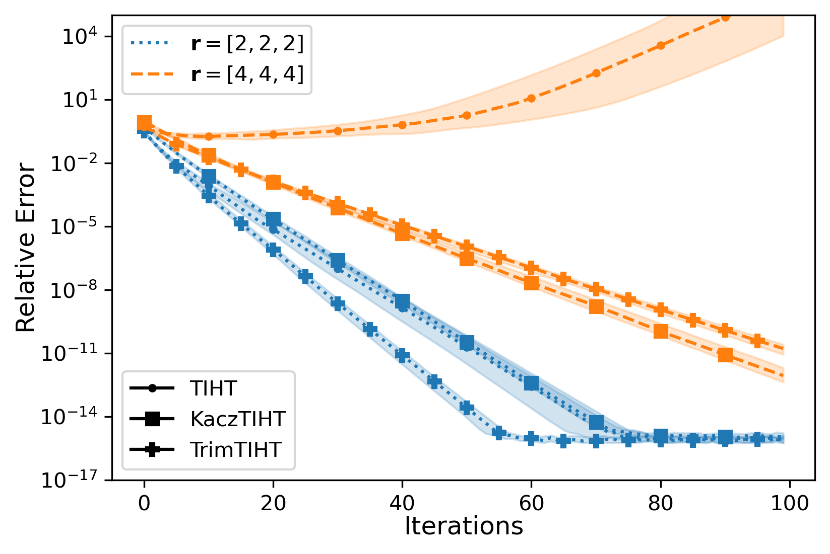
(a) HOSVD rank ${\bf r}$, $m=1000$ measurements

(b) CP rank $r$, $m=1000$ measurements

Figure 4. Recovery from Gaussian measurements: Relative error dynamic during the recovery with TIHT, KaczTIHT and TrimTIHT of the tensors of different low rank. KaczTIHT converges faster and to a lower error, especially for higher rank tensors, and TIHT starts diverging. The lines correspond to the median over $40$ sample runs, and the band represents the inter-quartile range.

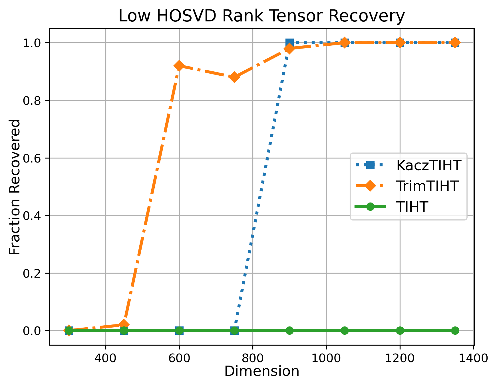
(a) HOSVD Rank (2,2,2)

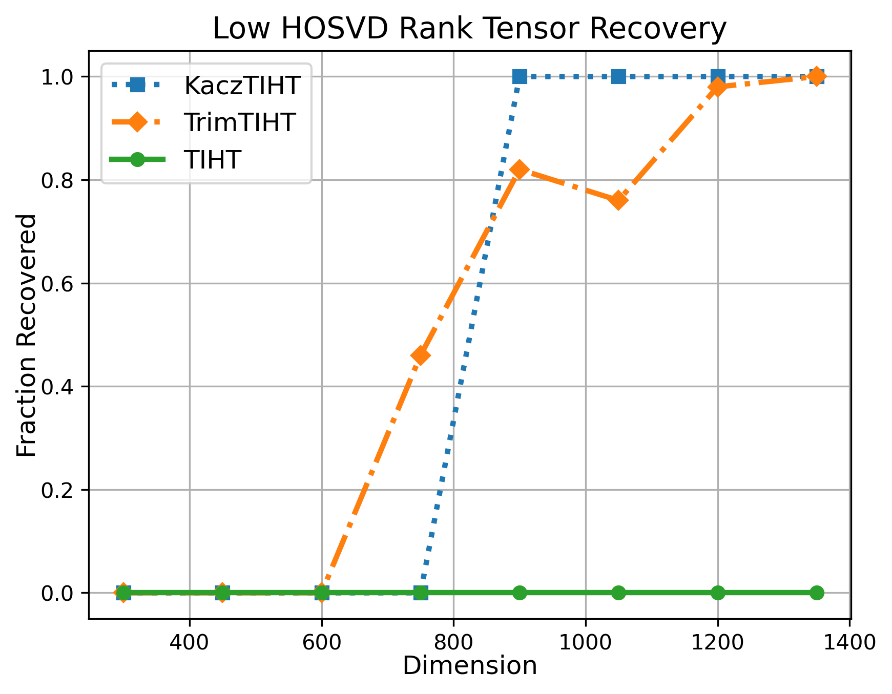
(b) HOSVD Rank (4,4,4)

(c) CP Rank 3

Figure 5. Recovery from face-splitting product of Gaussian measurements: Fraction of $50$ artificially generated random tensors of a certain rank, recovered successfully using TIHT, TrimTIHT and KaczTIHT from different levels of compression. The proposed methods enable successful recovery from memory-efficient measurements that is not achieved by TIHT.

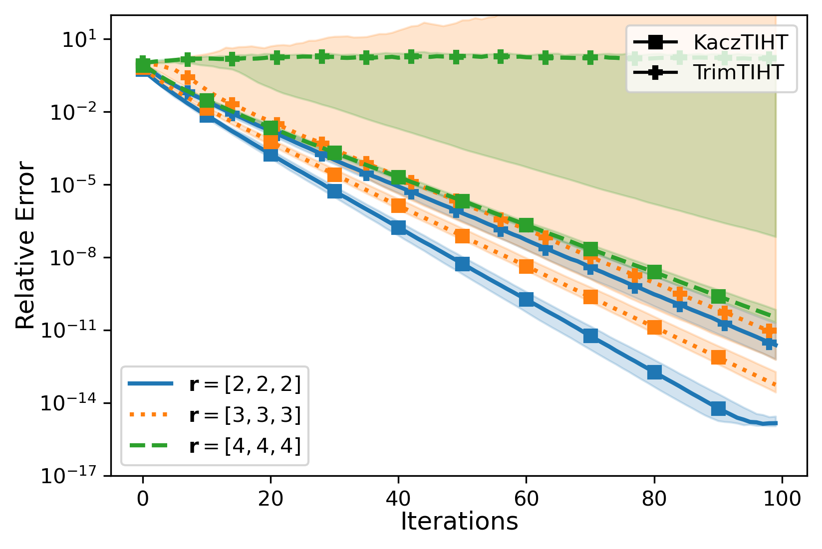
(a) HOSVD rank ${\bf r}$, $m=1350$ measurements

(b) CP rank $r$, $m=1500$ measurements

Figure 6. Recovery from face-splitting product of Gaussian measurements: Relative error dynamic during the recovery with KaczTIHT and TrimTIHT of the tensors of different low rank. KaczTIHT converges faster and to a lower error, especially for higher rank tensors. The lines correspond to the median over $40$ sample runs, and the band represents the interquartile range.

5.2. Recovery of Compressed Video Data

In this experiment, we apply our proposed methods to compress and recover a real-world video dataset. We use the video of a flickering candle flame from the Dynamic Texture Toolbox (http://www.vision.jhu.edu/code/). For more tractable computations, we consider only $10$ frames cropped to $30\times 30$ pixels around the center of the image. We compress the video tensor using i.i.d. Gaussian and face-splitting product of i.i.d. Gaussian measurement ensembles of dimensions $\mathbb{R}^{2700\times 9000}$ which correspond to $30\%$ compression. The original tensor is approximately of HOSVD rank $(8,9,5)$, with a relative error of low-rank tensor fitting via HOOI iteration (implemented in the Tensorly package) of $0.009$. Our goal is to recover this structure from data-oblivious measurements, that is a harder task than the HOSVD components recovery tailored for a particular dataset. Yet, with TrimTIHT and KaczTIHT methods we approach a compatible $10^{-2}$ relative error for the recovery from the data-oblivious measurements, as shown in Figure 7.

Specifically, in Figure 7, we plot the relative error with iterations of KaczTIHT and TrimTIHT ($m_{trim}=550$) for recovery from Gaussian measurements and from face-splitting measurements. Note that the face-splitting measurements take $128$ times less memory than unstructured i.i.d. measurements ($2700\times(30+30+10)\text{ vs. }2700\times(30\times 30\times 10)$ bits) to store, while allowing for essentially the same recovery properties.

In conclusion, both proposed methods are able to recover the original video almost to the best low-rank approximation error, and TIHT immediately diverged for both type of measurements, so it is not shown in the figure. KaczTIHT converges faster than TrimTIHT and this can be attributed to the relatively high rank of the problem.

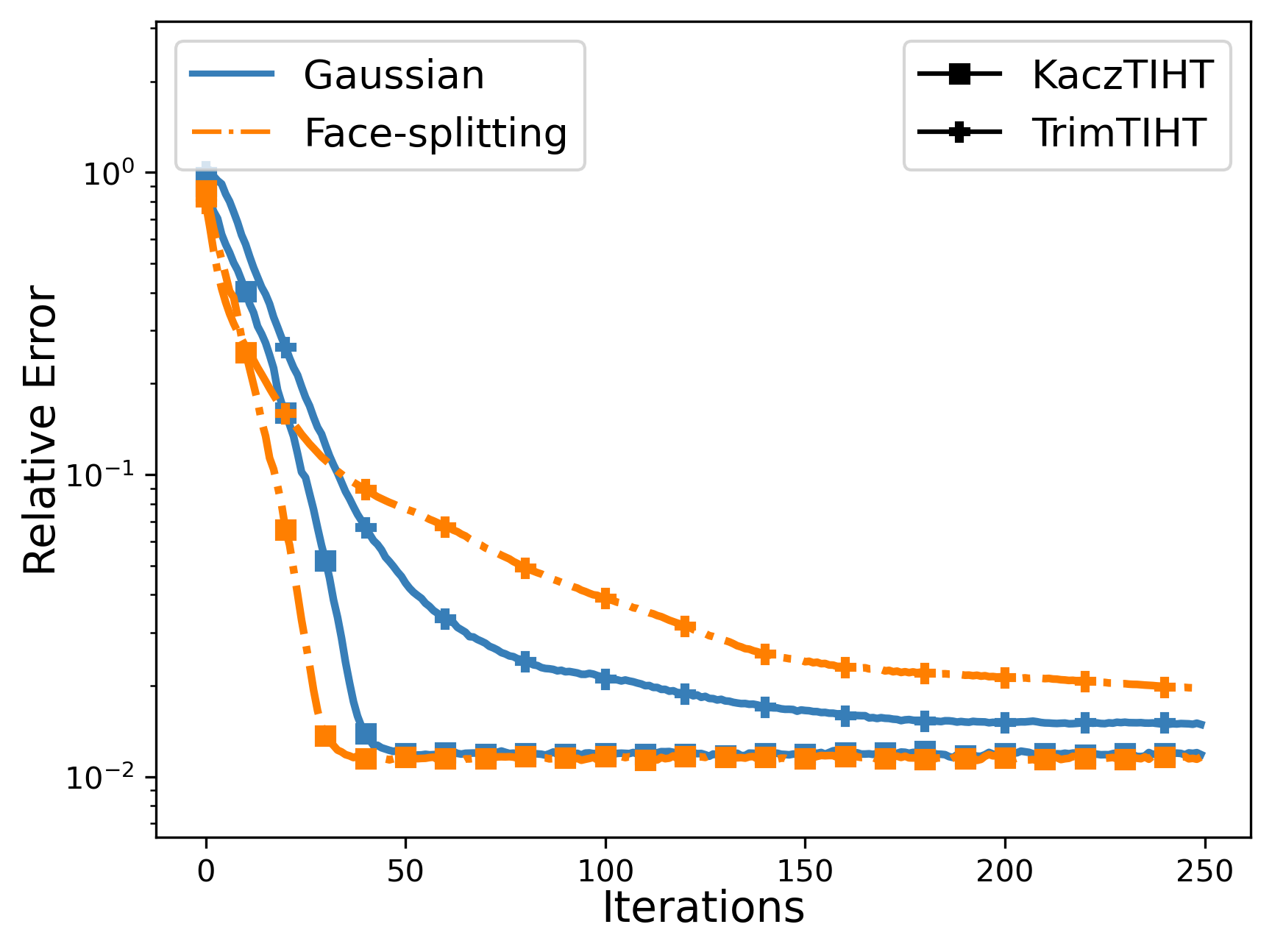
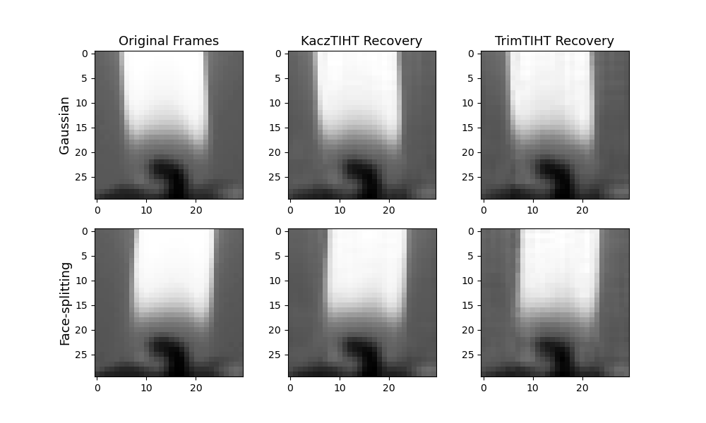
Figure 7. (Left) Relative error of recovered Candle video dataset using KaczTIHT and TrimTIHT from Gaussian and face-splitting measurements. The tensor is of relatively high rank $(9,8,5)$, the compression is to $30\%$ of its size. TIHT method immediately diverges on the same setup. The achieved relative error is compatible with $0.009$ HOSVD fitting error. (Right) The first frame of the original video and its recovered versions are presented in the first row, and the last frame and its recovered images are depicted in the bottom row.

6. Conclusions and Future Directions

In this paper, we aim to improve the performance of the standard tensor low-rank recovery methods, such as TensorIHT, especially in the hard cases when the rank is higher or the linear measurements are structured. We achieve this by proposing two efficient iterative hard thresholding-based methods – TrimTIHT and KaczTIHT – for low-rank tensor recovery, including HOSVD and CP ranks. We show that a class of practical structured and memory-efficient measurement operators, based on the face-splitting tensor product, fails to satisfy TensorRIP, a key property required to guarantee convergence for vanilla TensorIHT. Then, we analyze how local adaptive trimming of the measurements (the core idea of the proposed TrimTIHT method) can help in restoring TensorRIP-like guarantees for such database-friendly measurement operators. We also provide theoretical convergence guarantees for the proposed recovery methods and a suite of numerical experiments that showcase their efficacy, which is especially prominent in situations where we lack good TensorRIP properties.

There are multiple further questions stemming from this work. This includes providing theoretical evidence for the superior performance of the KaczTIHT method (this question seems to be unknown and interesting even for the sparse recovery counterpart of the method, see [60]). Adaptive trimming in Kaczmarz methods is known to also improve robustness, in particular, to avoid possibly corrupted measurements [54, 53], it would be natural to consider the effect of trimmed methods for the robust low-rank recovery problem. Additional next directions include utilizing adaptive trimming within other low-rank tensor processing methods, many of which also have TensorRIP requirements, making them ineffective for recovery from database-friendly measurements.

References

- [1] Carl Eckart and Gale Young “The approximation of one matrix by another of lower rank” In Psychometrika 1.3 Springer, 1936, pp. 211–218
- [2] Stefan Kaczmarz “Angenäherte Auflösung von Systemen linearer Gleichungen” In Bull. Int. Acad. Pol. Sic. Let., Cl. Sci. Math. Nat., 1937, pp. 355–357
- [3] Lieven De Lathauwer, Bart De Moor and Joos Vandewalle “A multilinear singular value decomposition” In SIAM journal on Matrix Analysis and Applications 21.4 SIAM, 2000, pp. 1253–1278
- [4] Lieven De Lathauwer, Bart De Moor and Joos Vandewalle “On the best rank-1 and rank-(r1, r2,…, rn) approximation of higher-order tensors” In SIAM journal on Matrix Analysis and Applications 21.4 SIAM, 2000, pp. 1324–1342
- [5] Pentti Paatero “Construction and analysis of degenerate PARAFAC models” In Journal of Chemometrics: A Journal of the Chemometrics Society 14.3 Wiley Online Library, 2000, pp. 285–299
- [6] Emmanuel J Candès, Justin Romberg and Terence Tao “Robust uncertainty principles: Exact signal reconstruction from highly incomplete frequency information” In IEEE Transactions on information theory 52.2 IEEE, 2006, pp. 489–509
- [7] Emmanuel J Candes “The restricted isometry property and its implications for compressed sensing” In Comptes rendus. Mathematique 346.9-10, 2008, pp. 589–592
- [8] Nir Ailon and Bernard Chazelle “The fast Johnson–Lindenstrauss transform and approximate nearest neighbors” In SIAM Journal on Computing 39.1 SIAM, 2009, pp. 302–322
- [9] Tamara G Kolda and Brett W Bader “Tensor decompositions and applications” In SIAM review 51.3 SIAM, 2009, pp. 455–500
- [10] Thomas Strohmer and Roman Vershynin “A randomized Kaczmarz algorithm with exponential convergence” In Journal of Fourier Analysis and Applications 15.2 Springer, 2009, pp. 262–278
- [11] Jian-Feng Cai, Emmanuel J Candès and Zuowei Shen “A singular value thresholding algorithm for matrix completion” In SIAM Journal on Optimization 20.4 SIAM, 2010, pp. 1956–1982
- [12] Anirban Dasgupta, Ravi Kumar and Tamás Sarlós “A sparse Johnson- Lindenstrauss transform” In Proceedings of the forty-second ACM symposium on Theory of computing, 2010, pp. 341–350
- [13] Ji Liu, Przemyslaw Musialski, Peter Wonka and Jieping Ye “Tensor completion for estimating missing values in visual data” In IEEE transactions on pattern analysis and machine intelligence 35.1 IEEE, 2012, pp. 208–220
- [14] Nick Vannieuwenhoven, Raf Vandebril and Karl Meerbergen “A new truncation strategy for the higher-order singular value decomposition” In SIAM Journal on Scientific Computing 34.2 SIAM, 2012, pp. A1027–A1052
- [15] Jared Tanner and Ke Wei “Normalized iterative hard thresholding for matrix completion” In SIAM Journal on Scientific Computing 35.5 SIAM, 2013, pp. S104–S125
- [16] Daniel M Kane and Jelani Nelson “Sparser Johnson- Lindenstrauss transforms” In Journal of the ACM (JACM) 61.1 ACM New York, NY, USA, 2014, pp. 1–23
- [17] T Tony Cai and Anru Zhang “ROP: Matrix recovery via rank-one projections” In The Annals of Statistics JSTOR, 2015, pp. 102–138
- [18] Andrzej Cichocki et al. “Tensor decompositions for signal processing applications: From two-way to multiway component analysis” In IEEE signal processing magazine 32.2 IEEE, 2015, pp. 145–163
- [19] Michael B Cohen et al. “Dimensionality reduction for k-means clustering and low rank approximation” In Proceedings of the forty-seventh annual ACM symposium on Theory of computing, 2015, pp. 163–172
- [20] José Henrique de M Goulart and Gérard Favier “An iterative hard thresholding algorithm with improved convergence for low-rank tensor recovery” In 2015 23rd European Signal Processing Conference (EUSIPCO), 2015, pp. 1701–1705 IEEE
- [21] Puxiao Han, Ruixin Niu and Yonina C Eldar “Modified distributed iterative hard thresholding” In 2015 IEEE International Conference on Acoustics, Speech and Signal Processing (ICASSP), 2015, pp. 3766–3770 IEEE
- [22] Zhuosheng Zhang, Yongchao Yu and Shumin Zhao “Iterative hard thresholding based on randomized Kaczmarz method” In Circuits, Systems, and Signal Processing 34 Springer, 2015, pp. 2065–2075
- [23] Kai Zhong, Prateek Jain and Inderjit S Dhillon “Efficient matrix sensing using rank-1 gaussian measurements” In Algorithmic Learning Theory: 26th International Conference, ALT 2015, Banff, AB, Canada, October 4-6, 2015, Proceedings 26, 2015, pp. 3–18 Springer
- [24] Woody Austin, Grey Ballard and Tamara G Kolda “Parallel tensor compression for large-scale scientific data” In 2016 IEEE international parallel and distributed processing symposium (IPDPS), 2016, pp. 912–922 IEEE
- [25] Yuejie Chi and Yue M Lu “Kaczmarz method for solving quadratic equations” In IEEE Signal Processing Letters 23.9 IEEE, 2016, pp. 1183–1187
- [26] Massimo Fornasier, Steffen Peter, Holger Rauhut and Stephan Worm “Conjugate gradient acceleration of iteratively re-weighted least squares methods” In Computational Optimization and Applications 65 Springer, 2016, pp. 205–259
- [27] Xian Guo et al. “Support tensor machines for classification of hyperspectral remote sensing imagery” In IEEE Transactions on Geoscience and Remote Sensing 54.6 IEEE, 2016, pp. 3248–3264
- [28] Evangelos E Papalexakis, Christos Faloutsos and Nicholas D Sidiropoulos “Tensors for data mining and data fusion: Models, applications, and scalable algorithms” In ACM Transactions on Intelligent Systems and Technology (TIST) 8.2 ACM New York, NY, USA, 2016, pp. 1–44
- [29] Ke Wei, Jian-Feng Cai, Tony F Chan and Shingyu Leung “Guarantees of Riemannian optimization for low rank matrix recovery” In SIAM Journal on Matrix Analysis and Applications 37.3 SIAM, 2016, pp. 1198–1222
- [30] Zemin Zhang and Shuchin Aeron “Exact tensor completion using t-SVD” In IEEE Transactions on Signal Processing 65.6 IEEE, 2016, pp. 1511–1526
- [31] Guoxu Zhou et al. “Linked component analysis from matrices to high-order tensors: Applications to biomedical data” In Proceedings of the IEEE 104.2 IEEE, 2016, pp. 310–331
- [32] Borbála Hunyadi, Patrick Dupont, Wim Van Paesschen and Sabine Van Huffel “Tensor decompositions and data fusion in epileptic electroencephalography and functional magnetic resonance imaging data” In Wiley Interdisciplinary Reviews: Data Mining and Knowledge Discovery 7.1 Wiley Online Library, 2017, pp. e1197
- [33] Holger Rauhut, Reinhold Schneider and Željka Stojanac “Low rank tensor recovery via iterative hard thresholding” In Linear Algebra and its Applications 523 Elsevier, 2017, pp. 220–262
- [34] Nicholas D Sidiropoulos et al. “Tensor decomposition for signal processing and machine learning” In IEEE Transactions on signal processing 65.13 IEEE, 2017, pp. 3551–3582
- [35] Casey Battaglino, Grey Ballard and Tamara G Kolda “A practical randomized CP tensor decomposition” In SIAM Journal on Matrix Analysis and Applications 39.2 SIAM, 2018, pp. 876–901
- [36] Roman Vershynin “High-dimensional probability: An introduction with applications in data science” Cambridge University Press, 2018
- [37] Shusen Wang, Alex Gittens and Michael W Mahoney “Sketched ridge regression: Optimization perspective, statistical perspective, and model averaging” In Journal of Machine Learning Research 18.218, 2018, pp. 1–50
- [38] Huishuai Zhang, Yuejie Chi and Yingbin Liang “Median-truncated nonconvex approach for phase retrieval with outliers” In IEEE Transactions on information Theory 64.11 IEEE, 2018, pp. 7287–7310
- [39] Thomas D Ahle and Jakob BT Knudsen “Almost optimal tensor sketch” In arXiv preprint arXiv:1909.01821, 2019
- [40] Rafael Ballester-Ripoll, Peter Lindstrom and Renato Pajarola “TTHRESH: Tensor compression for multidimensional visual data” In IEEE transactions on visualization and computer graphics 26.9 IEEE, 2019, pp. 2891–2903
- [41] Simon Foucart and Srinivas Subramanian “Iterative hard thresholding for low-rank recovery from rank-one projections” In Linear Algebra and its Applications 572 Elsevier, 2019, pp. 117–134
- [42] Jean Kossaifi, Yannis Panagakis, Anima Anandkumar and Maja Pantic “Tensorly: Tensor learning in python” In Journal of Machine Learning Research 20.26, 2019, pp. 1–6
- [43] Zhao Song, David P Woodruff and Peilin Zhong “Relative error tensor low rank approximation” In Proceedings of the Thirtieth Annual ACM-SIAM Symposium on Discrete Algorithms, 2019, pp. 2772–2789 SIAM
- [44] Thomas D Ahle et al. “Oblivious sketching of high-degree polynomial kernels” In Proceedings of the Fourteenth Annual ACM-SIAM Symposium on Discrete Algorithms, 2020, pp. 141–160 SIAM
- [45] Rachel Grotheer et al. “Stochastic iterative hard thresholding for low-Tucker-rank tensor recovery” In 2020 Information Theory and Applications Workshop (ITA), 2020, pp. 1–5 IEEE
- [46] Shahana Ibrahim, Xiao Fu and Xingguo Li “On recoverability of randomly compressed tensors with low CP rank” In IEEE Signal Processing Letters 27 IEEE, 2020, pp. 1125–1129
- [47] Roman Vershynin “Concentration inequalities for random tensors” In Bernoulli, 2020, pp. 3139–3162
- [48] Xuemei Chen and Jing Qin “Regularized Kaczmarz algorithms for tensor recovery” In SIAM Journal on Imaging Sciences 14.4 SIAM, 2021, pp. 1439–1471
- [49] Mark A Iwen, Deanna Needell, Elizaveta Rebrova and Ali Zare “Lower memory oblivious (tensor) subspace embeddings with fewer random bits: modewise methods for least squares” In SIAM Journal on Matrix Analysis and Applications 42.1 SIAM, 2021, pp. 376–416
- [50] Ruhui Jin, Tamara G Kolda and Rachel Ward “Faster Johnson–Lindenstrauss transforms via Kronecker products” In Information and Inference: A Journal of the IMA 10.4 Oxford University Press, 2021, pp. 1533–1562
- [51] Yiming Sun, Yang Guo, Joel A Tropp and Madeleine Udell “Tensor random projection for low memory dimension reduction” In arXiv preprint arXiv:2105.00105, 2021
- [52] Kyriakos Axiotis and Maxim Sviridenko “Iterative hard thresholding with adaptive regularization: Sparser solutions without sacrificing runtime” In International Conference on Machine Learning, 2022, pp. 1175–1197 PMLR
- [53] Lu Cheng, Benjamin Jarman, Deanna Needell and Elizaveta Rebrova “On block accelerations of quantile randomized Kaczmarz for corrupted systems of linear equations” In Inverse Problems 39.2 IOP Publishing, 2022, pp. 024002
- [54] Jamie Haddock, Deanna Needell, Elizaveta Rebrova and William Swartworth “Quantile-based iterative methods for corrupted systems of linear equations” In SIAM Journal on Matrix Analysis and Applications 43.2 SIAM, 2022, pp. 605–637
- [55] Qijia Jiang “Near-isometric properties of Kronecker-structured random tensor embeddings” In Advances in Neural Information Processing Systems 35, 2022, pp. 10191–10202
- [56] Zoraida Fernández Rico “Optimal statistical estimation: sub-Gaussian properties, heavy-tailed data, and robust-ness”, 2022
- [57] Rachel Grotheer et al. “Iterative singular tube hard thresholding algorithms for tensor recovery” In arXiv preprint arXiv:2304.04860, 2023
- [58] Cullen Haselby et al. “Fast and Low-Memory Compressive Sensing Algorithms for Low Tucker-Rank Tensor Approximation from Streamed Measurements” In arXiv preprint arXiv:2308.13709, 2023
- [59] Cullen A Haselby et al. “Modewise operators, the tensor restricted isometry property, and low-rank tensor recovery” In Applied and Computational Harmonic Analysis 66 Elsevier, 2023, pp. 161–192
- [60] Halyun Jeong and Deanna Needell “Linear Convergence of Reshuffling Kaczmarz Methods With Sparse Constraints” In arXiv preprint arXiv:2304.10123, 2023
- [61] Yuetian Luo and Anru R Zhang “Low-rank tensor estimation via Riemannian Gauss-Newton: Statistical optimality and second-order convergence” In The Journal of Machine Learning Research 24.1 JMLRORG, 2023, pp. 18274–18321
- [62] Yifan Zhang and Joe Kileel “Covering Number of Real Algebraic Varieties and Beyond: Improved Bounds and Applications” In arXiv e-prints, 2023, pp. arXiv–2311
- [63] Grey Ballard and Tamara G Kolda “Tensor Decompositions for Data Science” Cambridge University Press, 2025