Beyond Topological Self-Explainable GNNs:
A Formal Explainability Perspective

Abstract

Self-Explainable Graph Neural Networks (SE-GNNs) are popular explainable-by-design GNNs, but the properties and the limitations of their explanations are not well understood. Our first contribution fills this gap by formalizing the explanations extracted by SE-GNNs, referred to as Trivial Explanations (TEs), and comparing them to established notions of explanations, namely Prime Implicant (PI) and faithful explanations. Our analysis reveals that TEs match PI explanations for a restricted but significant family of tasks. In general, however, they can be less informative than PI explanations and are surprisingly misaligned with widely accepted notions of faithfulness. Although faithful and PI explanations are informative, they are intractable to find and we show that they can be prohibitively large. Motivated by this, we propose Dual-Channel GNNs that integrate a white-box rule extractor and a standard SE-GNN, adaptively combining both channels when the task benefits. Our experiments show that even a simple instantiation of Dual-Channel GNNs can recover succinct rules and perform on par or better than widely used SE-GNNs. Our code can be found in the supplementary material.

1 Introduction

Self-Explainable GNNs (SE-GNNs) are Graph Neural Networks (Scarselli et al., 2008; Wu et al., 2020b) designed to combine high performance and ante-hoc interpretability. In a nutshell, a SE-GNN integrates two GNN modules: an explanation extractor responsible for identifying a class-discriminative subgraph of the input and a classifier mapping said subgraph onto a prediction. Since this subgraph, taken in isolation, is enough to infer the prediction, it plays the role of a local explanation thereof. Despite the popularity of SE-GNNs (Miao et al., 2022a; Lin et al., 2020; Serra & Niepert, 2022; Zhang et al., 2022; Ragno et al., 2022; Dai & Wang, 2022), little is known about the properties and limitations of their explanations. Our work fills this gap.

Focusing on graph classification, we show that popular SE-GNNs are implicitly optimized for generating Trivial Explanations (TEs), i.e., minimal subgraphs of the input that locally ensure the classifier outputs the target prediction. Then we compare TEs with two other families of formal explanations: Prime Implicant explanations (PIs) and faithful explanations. Faithful explanations are subgraphs that are sufficient and necessary for justifying a prediction, i.e., they capture all and only those elements that cause the predicted label (Yuan et al., 2022; Tan et al., 2022; Agarwal et al., 2023; Azzolin et al., 2024). PIs, instead, are minimally sufficient explanations extensively studied in formal explainability of tabular and image data (Marques-Silva, 2023; Darwiche & Hirth, 2023; Wang et al., 2021). They are also highly informative, e.g., for any propositional formula the set of PIs is enough to reconstruct the original formula (Ignatiev et al., 2015). Moreover, both PI and sufficient explanations are tightly linked to counterfactuals (Beckers, 2022) and adversarial robustness (Ignatiev et al., 2019).

Our results show that TEs match PI explanations in the restricted but important family of motif-based prediction tasks, where labels depend on the presence of topological motifs. Although in these tasks TEs inherit all benefits of PIs, in general they are neither faithful nor PIs.

Motivated by this, we introduce Dual-Channel GNNs (DC-GNNs), a novel family of SE-GNNs that aim to extend the perks of motif-based tasks to more general settings. DC-GNNs combine a SE-GNN and a non-relational white-box predictor, adaptively employing one or both depending on the task. Intuitively, the non-relational channel handles non-topological aspects of the input, leaving the SE-GNN free to focus on topological motifs with TEs. This setup encourages the corresponding TEs to be more compact, all while avoiding the (generally exponential (Marques-Silva, 2023)) computational cost of extracting PIs explicitly. Empirical results on three synthetic and five real-world graph classification datasets highlight that DC-GNNs perform as well or better than SE-GNNs by adaptively employing one channel or both depending on the task.

Contributions. Summarizing, we:

• Formally characterize the class of explanations that SE-GNNs optimize for, namely TEs.

• Show that TEs share key properties of PI and faithful explanations for motif-based prediction tasks.

• Propose Dual-Channel GNNs and compare them empirically to representative SE-GNNs, highlighting their promise in terms of explanation size and performance.

2 Preliminaries

We will use $g$ to represent a graph classifier, usually representing a GNN. Given a graph $G=(V,E)$, we will use $g(G)$ to denote $g$’s predicted label on $G$. Additionally, graphs can be annotated with edge or node features. Throughout, we will use the notation $R\subset G$ to denote that $R$ is a subgraph of $G$ and $R\subseteq G$ to denote that $R$ may be a subgraph or $G$ itself. Note that we assume that a subgraph $R\subseteq G$ can contain all, less, or none of the features of the nodes (or edges) in $G$. We will use $|G|$ to indicate the size of the graph $G$. The size may be defined in terms of the number of nodes, edges, features, or their combination, and the precise semantics will be clear from the context.

Self-explainable GNNs. SE-GNNs are designed to complement the high performance of regular GNNs with ante-hoc interpretability. They pair an explanation extractor $q$ mapping the input $G$ to a subgraph $q(G)=R\subseteq G$ playing the role of a local explanation, and a classifier $f$ using $R$ to infer a prediction:

$$g(G)=f(q(G))$$ (1)

In practice, the explanation extractor $q$ outputs per-edge relevance scores $p_{uv}\in\mathbb{R}$, which are translated into an edge-induced subgraph $R$ via thresholding (Yu et al., 2022) or top-$k$ selection (Miao et al., 2022a; Chen et al., 2024). While we focus on per-edge relevance scores due to their widespread use, our results equally apply to per-node relevance scores (Miao et al., 2022a).

Approaches for training SE-GNNs are designed to extract an interpretable subgraph that suffices to produce the target prediction, often formalized in terms of sparsity regularization (Sparsity) (Lin et al., 2020; Serra & Niepert, 2022) or the Information Bottleneck (IB) (Tishby et al., 2000). Since the exact IB is intractable and difficult to estimate (Kraskov et al., 2004; McAllester & Stratos, 2020), common approaches devise bounds on the divergence between the relevance scores and an uninformative prior controlled by the parameter $r\in[0,1]$ (Miao et al., 2022a, b). This work focuses on representative training objectives for both Sparsity- and IB-based SE-GNNs, indicated in Table˜1.

Logical classifiers. We will use basic concepts from First-Order Logic (FOL) as described in Barceló et al. (2020) and Grohe (2021), and use $E(x,y)$ to denote an undirected edge between $x$ and $y$. A FOL boolean classifier is a FOL sentence $\Phi$ that labels an instance $G$ positively if $G\models\Phi$ and negatively otherwise. We present two examples of FOL classifiers that will be relevant to our discussion: $\exists x\exists y.E(x,y)$ classifies a graph positively if it has an edge, while $\forall x\exists y.E(x,y)$ when it has no isolated nodes. Note that both can be expressed by a GNN, as they are in the logical fragment $\mathrm{C}^{2}$ (see Theorem IX.3 in Grohe (2021)). We say that two classifiers are distinct if there exists at least one instance where their predictions differ. Although most of our results discuss general graph classifiers, they equally apply to the specific case of GNNs.

Model	Group	Learning Objective
GISST (Lin et al., 2020)	Sparsity	$\mathcal{L}+\frac{\lambda_{1}}{|E|}\sum_{(u,v)\in E}p_{uv}+\frac{\lambda_{2}}{|E|}\sum_{(u,v)\in\mathcal{E}}p_{uv}\log(p_{uv})+(1-p_{uv})\log(1-p_{uv})$
GSAT, LRI (Miao et al., 2022a, b), GMT (Chen et al., 2024)	IB	$\mathcal{L}+\lambda_{1}\sum_{(u,v)\in E}p_{uv}\log(\frac{p_{uv}}{r})+(1-p_{uv})\log(\frac{1-p_{uv}}{1-r})$

Table 1: Training objectives of popular SE-GNNs. $\mathcal{L}$ is the cross-entropy loss between model predictions $f(q(G))$ and target variable $Y$. Theorem˜3.2 shows that all of them optimize for generating Trivial Explanations (Definition˜3.1).

3 What are SE-GNN Explanations?

Despite being tailored for explainability, SE-GNNs lack a precise description of the properties of the explanations they extract. In this section, we present a formal characterization (in Definition˜3.1) of explanations extracted by SE-GNNs, called Trivial Explanations (TEs). In Theorem˜3.2 we show that, for an SE-GNN with perfect predictive accuracy and a hard explanation extractor, the loss functions in Table˜1 are minimal iff the explanation $R$ is a TE.

Definition 3.1 (Trivial Explanations).

Let $g$ be a graph classifier and $G$ be an instance with predicted label $g(G)$, then $R$ is a Trivial Explanation for $g(G)$ if:

1. $R\subseteq G$

2. $g(G)=g(R)$

3. There does not exist an explanation $R^{\prime}\subseteq G$ such that $|R^{\prime}|<|R|$ and $g(G)=g(R^{\prime})$.

Trivial Explanations are not unique, and we use $\mathrm{TE}(g(G))$ to denote the set of all trivial explanations for $g(G)$.

Since our goal is to formally analyze explanations extracted by SE-GNNs, we make idealized assumptions about the classifier $f$. Hence, we assume that the SE-GNN is expressive enough and attains perfect predictive accuracy, i.e., it always returns the correct label for $G$. We also assume that it learns a hard explanation extractor, i.e., $q$ outputs scores saturated to $\{0,1\}$ (Yu et al., 2020). Under these assumptions, we show that SE-GNNs in Table˜1 optimize for generating TEs.

Theorem 3.2.

Let $g$ be an SE-GNN with a ground truth classifier $f$ (i.e., $f(G)$ always returns the true label for $G$), a hard explanation extractor $q$, and perfect predictive accuracy. Then, $g$ achieves minimal true risk (as indicated in Table 1) if and only if for any instance $G$, $q(G)$ provides Trivial Explanations for the predicted label $g(G)$.

Proof Sketch.

For a hard explanation extractor $q$, the risk terms in Table˜1 reduce to $\mathcal{L}(f(q(G)),Y)+\lambda_{1}|q(G)|/|E|$ and $\mathcal{L}(f(q(G),Y)+\lambda_{1}|q(G)|\log(r^{-1})$. Since the SE-GNN attains perfect predictive accuracy, $\mathcal{L}(f(q(G)),Y)$ is minimal. Hence, for both cases, the total risk is minimized when $q(G)$ is the smallest subgraph that preserves the label, i.e., a Trivial Explanation. ∎

Proofs relevant to the discussion are reported in the main text, while the others are available in Appendix˜A.

Remark 3.3.

A simple desideratum for any type of explanation is that it gives information about the classifier beyond the predicted label. A weak formulation of this desideratum is that explanations for two distinct classifiers should differ for at least one instance where they predict the same label.

The following theorem, however, shows that TEs can fail to satisfy this desideratum for general prediction tasks.

Theorem 3.4.

There exist two distinct classifiers $g$ and $g^{\prime}$ such that for any $G$ where $g(G)=g^{\prime}(G)$ we have that

$$\mathrm{TE}(g(G))=\mathrm{TE}(g^{\prime}(G))$$ (2)

Proof.

Let $g$ and $g^{\prime}$ be boolean graph classifiers given by FOL formulas $g=\exists x\exists y.E(x,y)$ and $g^{\prime}=\forall x\exists y.E(x,y)$ respectively. Let $G$ be any positive instance for both $g$ and $g^{\prime}$, and let $E$ and $V$ be the set of edges and nodes in $G$, respectively. For any $e\in E$, we have that $e$ is a Trivial Explanation for both $g(G)$ and $g^{\prime}(G)$ (e.g. see Fig.˜1). Hence, $\mathrm{TE}(g(G))=\mathrm{TE}(g^{\prime}(G))=E$. Similarly, if $G$ is a negative instance for both $g$ and $g^{\prime}$, we have that a Trivial Explanation is a subgraph consisting of any single node from $G$, and $\mathrm{TE}(g(G))=\mathrm{TE}(g^{\prime}(G))=V$. ∎

Theorem˜3.4 highlights additional insights worth discussing. Consider again the classifier $g^{\prime}=\forall x\exists y.E(x,y)$, and let $G$ be a negative instance for $g^{\prime}$ composed of three nodes $\{u_{1},u_{2},u_{3}\}$, only two of which are connected by the edge $(u_{1},u_{2})\in E$. In this case, a user may expect to see the isolated node $u_{3}$ as an explanation. However, any subgraph consisting of a single isolated node from the set $\{u_{1},u_{2},u_{3}\}$ is a valid TE. This highlights that as TEs focus only on the subgraphs allowing the model to reproduce the same prediction, they may lead to counter-intuitive explanations.

Furthermore, Theorem˜3.4 implies that

$$\textstyle\bigcup_{G\in\Omega^{(y)}}\mathrm{TE}(g(G))=\bigcup_{G\in\Omega^{(y)}}\mathrm{TE}(g^{\prime}(G))$$ (3)

where $\Omega^{(y)}$ is the set of all instances $G$ such that $g(G)=g^{\prime}(G)=y$, $g=\exists x\exists y.E(x,y)$, and $g^{\prime}$ is as above. Hence, there exist classifiers where model-level explanations built by aggregating over multiple local explanations (Setzu et al., 2021; Azzolin et al., 2022) may also not be informative w.r.t. Remark˜3.3. In the next section, we investigate a widely accepted formal notion of explanations, namely Prime Implicant explanations (PIs), for graph classifiers. We analyze the informativeness of TEs compared to PIs and characterize when they match.

4 Trivial and Prime Implicant Explanations

In this section, we provide a formal comparative analysis between Trivial and PI explanations for graph classifiers. While PIs are extensively studied for tabular and image-like data (Marques-Silva et al., 2020; Marques-Silva, 2023), little investigation has been carried out for graphs. Our analysis shows that TEs match PIs for a large class of tasks – those based on the recognition of motifs – but they do not align in general. We also show that PIs are more informative than TEs w.r.t the desideratum in Remark˜3.3.

Let us start by defining PIs for graph classifiers.

Definition 4.1 (PI explanation).

Let $g$ be a classifier and $G$ be an instance with predicted label $g(G)$, then $R$ is a Prime Implicant explanation for $g(G)$ if:

1. $R\subseteq G$.

2. For all $R^{\prime}$, such that $R\subseteq R^{\prime}\subseteq G$, we have that ${g(G)=g(R^{\prime})}$.

3. No other $R^{\prime}\subset R$ satisfies both (1) and (2).

Like TEs, PIs are not unique, and we use $\mathrm{PI}(g(G))$ to denote the set of all PIs for $g(G)$.

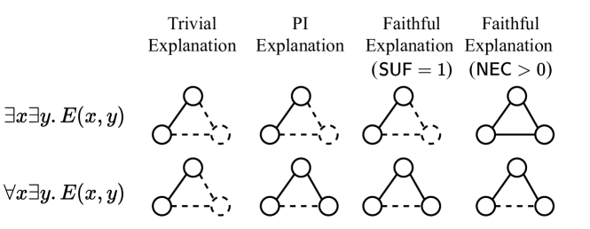
Figure 1: Examples of a Trivial, PI, and faithful explanation (w.r.t Proposition˜5.3 and Proposition˜5.4) for the predictions of $\exists x\exists y.E(x,y)$ and $\forall x\exists y.E(x,y)$ on a triangle.

PIs feature several nice properties, in that they are guaranteed to be the minimal explanations that are provably sufficient for the prediction (Shih et al., 2018; Beckers, 2022; Darwiche & Hirth, 2023). To illustrate the difference between TEs and PIs, we provide examples of both in Fig.˜1 for two different classifiers on the same instance. Note that for the classifier $\exists x\exists y.E(x,y)$, TEs match PIs. This observation indeed generalizes to all existentially quantified FOL formulas, as shown next.

4.1 TEs Match PI for Existential Classifiers

Theorem 4.2.

Given a classifier $g$ expressible as a purely existentially quantified first-order logic formula and a positive instance $G$ of any size, then a Trivial Explanation for $g(G)$ is also a Prime Implicant explanation for $g(G)$.

Proof sketch..

A purely existentially quantified FOL formula $g$ is of the form $\exists x_{1},\dots,\exists x_{k}.\Phi(x_{1},\dots,x_{k})$, where $\Phi$ is quantifier-free. For a positive instance $G$, a Trivial Explanation is the smallest subgraph $R$ induced by nodes in a tuple $\bar{a}=(a_{1},\dots,a_{k})$, such that $\Phi(\bar{a})$ holds. Now, any supergraph of $R$ necessarily contains $\bar{a}$, and hence witnesses $\exists x_{1},\dots,\exists x_{k}.\Phi(x_{1},\dots,x_{k})$, while any smaller subgraph violates $\exists x_{1},\dots,\exists x_{k}.\Phi(x_{1},\dots,x_{k})$, as $\bar{a}$ is minimal by construction. Hence, $R$ is a PI. ∎

Note that tasks based on the recognition of a topological motif (like the existence of a star) can indeed be cast as existentially quantified formulas ($\exists xyzw.E(x,y)\land E(x,z)\land E(x,w)\land x\neq y\neq z\neq w$), qualifying TEs as ideal targets for those tasks. Motif-based tasks are indeed useful in a large class of practically relevant scenarios (Sushko et al., 2012; Jin et al., 2020; Chen et al., 2022; Wong et al., 2024), and have been a central assumption in many works on GNN explainability (Ying et al., 2019; Miao et al., 2022a; Wu et al., 2022). Theorem˜4.2 theoretically supports using SE-GNNs for these tasks, and shows they optimize for minimally sufficient explanations (PIs). However, global properties such as long-range dependencies (Gravina et al., 2022) or classifiers like $\forall x\exists yE(x,y)$, cannot be expressed by purely existential statements. In such scenarios, PIs can be more informative than TEs, as we show next.

4.2 TEs are Not More Informative than PIs

We begin by showing that TEs are not more informative than PIs w.r.t. Remark˜3.3.

Proposition 4.3.

Let $g$ be a classifier and $y$ a given label. Let $\Omega^{(y)}_{g}$ be the set of all the finite graphs (potentially with a given bounded size) with predicted label $y$. Then,

$$\textstyle\bigcup_{G\in\Omega^{(y)}_{g}}\mathrm{TE}(g(G))\ \subseteq\ \bigcup_{G\in\Omega^{(y)}_{g}}\mathrm{PI}(g(G))$$ (4)

This result shows that when considering the union of all finite graphs, PIs subsume TEs. Hence, if two classifiers share all PIs then they necessarily share all TEs as well, meaning that TEs do not provide more information about the underlying classifier than PIs. Conversely, we show that there exist cases where PIs provide strictly more information about the underlying classifier than TEs.

Theorem 4.4.

There exist two distinct classifiers $g$ and $g^{\prime}$ and a label $y$ such that:

1. For all graphs $G$ s.t. $g(G)=g^{\prime}(G)=y$, we have

   $$\mathrm{TE}\bigl{(}g(G)\bigr{)}\;=\;\mathrm{TE}\bigl{(}g^{\prime}(G)\bigr{)}.$$ (5)

2. There exists at least one graph $G^{\ast}$ with $g(G^{\ast})=g^{\prime}(G^{\ast})=y$ such that

   $$\mathrm{PI}\bigl{(}g(G^{\ast})\bigr{)}\;\neq\;\mathrm{PI}\bigl{(}g^{\prime}(G^{\ast})\bigr{)}.$$ (6)

We provide an example in Fig.˜1 of two classifiers where TEs are always equal for positive instances, but PIs are not.

Summarizing, TEs match PIs for motif-based tasks, and as such they inherit desirable properties of PIs. In the other cases, TEs can generally be less informative.

5 Trivial Explanations can be Unfaithful

A widespread approach to estimate the trustworthiness of an explanation is faithfulness (Yuan et al., 2022; Amara et al., 2022; Agarwal et al., 2023; Longa et al., 2024), which consists in checking whether the explanation contains all and only the elements responsible for the prediction. Clearly, unfaithful explanations fail to convey actionable information about what the model is doing to build its predictions (Agarwal et al., 2024). This section reviews a general notion of faithfulness (Azzolin et al., 2024) in Definition˜5.1, and shows that faithfulness and TEs can overlap – in some restricted cases – but are generally fundamentally misaligned.

Intuitively, faithfulness metrics assess how much the prediction changes when perturbing either the complement – referred to as sufficiency of the explanation – or the explanation itself – referred to as necessity of the explanation. Perturbations are sampled from a distribution of allowed modifications, which typically include edge and node removals. Then, an explanation is said to be faithful when it is both sufficient and necessary.

Definition 5.1 (Faithfulness).

Let $R\subseteq G$ be an explanation for $g(G)$ and $C=G\setminus R$ its complement. Let $p_{R}$ be a distribution over perturbations to $C$, and $p_{C}$ be a distribution over perturbations to $R$. Also, let $\Delta(G,G^{\prime})=\mathbbm{1}\!\left\{g(G)\neq g(G^{\prime})\right\}$ indicate a change in the predicted label. Then, $\mathsf{Suf}$ and $\mathsf{Nec}$ compute respectively the degree of sufficiency and degree of necessity of an explanation $R$ for a decision $g(G)$ as:

$$\mathsf{Suf}(R)=\exp(-\mathbb{E}_{G^{\prime}\sim p_{R}}[\Delta(G,G^{\prime})]),$$ (7)

$$\mathsf{Nec}(R)=1-\exp(-\mathbb{E}_{G^{\prime}\sim p_{C}}[\Delta(G,G^{\prime})]).$$ (8)

The degree of faithfulness $\mathsf{Faith}(R)$ is then the harmonic mean of $\mathsf{Suf}$ and $\mathsf{Nec}$.

The (negated) exponential normalization ensures that $\mathsf{Suf}$ (resp. $\mathsf{Nec}$) increases for more sufficient (resp. necessary) explanations. Note that both $\mathsf{Suf}$ and $\mathsf{Nec}$ need to be non-zero for a $\mathsf{Faith}$ score above zero. According to this definition, the degree of necessity will be high when many perturbations of $R$ lead to a prediction change and is thus $1$ when all of them do so. $\mathsf{Suf}$ is analogous.

As the next theorem shows, TEs can surprisingly fail in being faithful even for trivial tasks.

Theorem 5.2.

There exist tasks where Trivial Explanations achieve a zero degree of faithfulness.

Proof.

Let $g=\exists x\exists y.E(x,y)$ and $G$ a positive instance with more than one edge. Then, a Trivial Explanation $R$ consisting of a single edge (see Fig.˜1) achieves a $\mathsf{Nec}(R)$ value of zero, as any perturbations to $R$ will leave $G\setminus R$ unchanged. Hence, $g$ remains satisfied, meaning that $\mathsf{Nec}(R)=0$ and thus $\mathsf{Faith}(R)=0$. ∎

Note that $\exists x\exists y.E(x,y)$ achieves non-zero $\mathsf{Nec}(R)$ iff $R$ contains every edge, whereas $\mathsf{Suf}(R)=1$ is guaranteed by the presence of a single edge. These observations indeed generalize, as shown next.

Proposition 5.3.

An explanation $R\subseteq G$ for $g(G)$ has a maximal $\mathsf{Suf}(R)$ score if and only if there exists a PI explanation $M\subseteq R$ for $g(G)$.

Proposition 5.4.

An explanation $R\subseteq G$ for $g(G)$ has a non-zero $\mathsf{Nec}(R)$ score if and only if it intersects every PI explanation $M\subseteq R$ for $g(G)$.

Note that Proposition˜5.3 (along with Theorem˜4.2) show that TEs are indeed maximally sufficient for existentially quantified FOL formulas. However, this might not be enough to ensure a non-zero $\mathsf{Faith}$ score, as shown in Proposition˜5.4. In general, TEs highlight a minimal class-discriminative subgraph, whereas faithful explanations highlight all possible causes for the prediction, and the two notions are fundamentally misaligned.

6 Beyond (purely) Topological SE-GNNs

Our analysis highlights that explanations extracted by SE-GNNs can be, in general, both ambiguous (Theorem˜3.4) and unfaithful (Theorem˜5.2), potentially limiting their usefulness for debugging (Teso et al., 2023; Bhattacharjee & von Luxburg, 2024; Fontanesi et al., 2024), scientific discovery (Wong et al., 2024), and Out-of-Distribution (OOD) generalization (Chen et al., 2022; Gui et al., 2023). Nonetheless, we also showed that for a specific class of tasks, precisely those based on the presence of motifs, TEs are actually an optimal target, in that they match PIs and are the minimal explanations that are also provably sufficient (Theorem˜4.2 and Proposition˜5.3).

As PI and faithful explanations can generally be more informative than TEs (Proposition˜4.3 and Theorem˜4.4), one might consider devising SE-GNNs that always optimize for them. We argue, however, that aiming for PI or faithful explanations can be suboptimal, as they can be large and complex in the general case. For example, a PI explanation for a positive instance of $\forall x\exists y.E(x,y)$ is an edge cover (Weisstein, 2025), which grows with the size of the instance. Similarly, the explanation with an optimal faithfulness score for $\exists x\exists y.E(x,y)$ is the whole graph. Furthermore, finding and checking such explanations is inherently intractable, as both involve checking the model’s output on all possible subgraphs (Yuan et al., 2021). These observations embody the widely observed phenomenon that explanations can get as complex as the model itself (Rudin, 2019).

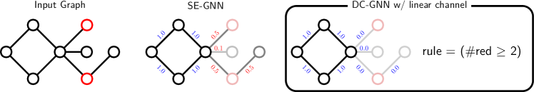
Figure 2: Illustration of our Dual-Channel architecture for a positive instance of TopoFeature, where positive instances contain a cycle and at least two red nodes. Numbers indicate edge relevance scores. SE-GNNs may fail to highlight precisely the elements relevant to the prediction, as the task involves non-topological patterns. DC-GNNs, instead, provide more focused topological explanations by offloading part of the prediction to interpretable rules (cf. Fig.˜7 and Fig.˜10).

6.1 Dual-Channel GNNs

This motivates us to investigate Dual-Channel GNNs (DC-GNNs), a new family of SE-GNNs aiming to preserve the perks of TEs for motif-based tasks while freeing them from learning non-motif-based patterns, which would be inefficiently represented as a subgraph. To achieve this, DC-GNNs pair an SE-GNN-based topological channel – named $\mathsf{Topo}$– with an interpretable channel – named $\mathsf{Rule}$– providing succinct non-topological rules. To achieve optimal separation of concerns while striving for simplicity, we jointly train the two channels and let DC-GNNs adaptively learn how to exploit them.

Definition 6.1.

(DC-GNN) Let $g_{1}:G\mapsto[0,1]^{n_{1}}$ be a SE-GNN, $g_{2}:G\mapsto[0,1]^{n_{2}}$ an interpretable model of choice, and $\mathsf{aggr}:[0,1]^{n_{1}+n_{2}}\mapsto Y$ an aggregation function. A DC-GNN is defined as:

$$g(G)=\mathsf{aggr}\big{(}g_{1}(G),g_{2}(G)\big{)}.$$ (9)

While the second channel $g_{2}$ can be any interpretable model of choice, we will experimentally show that even a simple sparse linear model can bring advantages over a standard SE-GNN, leaving the investigation of a more complex architecture to future work. Therefore, in practice, we will experiment with

$$\textstyle g_{2}(G)=\sigma\big{(}W\sum_{u\in G}x_{u}\big{)},$$ (10)

where $x_{u}\in\mathbb{R}^{d}$ is the node feature vector of $u$, $W\in\mathbb{R}^{n_{2}\times d}$ the weights of the linear model, and $\sigma$ is an element-wise sigmoid activation function. Also, we will fix $n_{1}=n_{2}$ equal to the number of classes of $Y$. In the experiments, we will promote a sparse $W$ via weight decay.

A key component of DC-GNNs is the $\mathsf{aggr}$ function joining the two channels. To preserve the interpretability of the overall model, $\mathsf{aggr}$ should act as a gateway for making the final predictions based on a simple combination of the two channels. To achieve this while ensuring differentiability, we considered an extension of Logic Explained Networks (LENs) (Barbiero et al., 2022), described below.

Implementing $\mathsf{aggr}$. LENs are small Multi-layer Perceptrons (MLP) taking as input a vector of activations in $[0,1]$ (Barbiero et al., 2022). The first layer of the MLP is regularized to identify the most relevant inputs while penalizing irrelevant ones via an attention mechanism. To promote the network to achieve discrete activations scores without resorting to high-variance reparametrization tricks (Azzolin et al., 2022; Giannini et al., 2024), we propose augmenting LENs with a progressive temperature annealing of the input vector. We validate the effectiveness of this extension in preserving the semantics of each channel, together with a comparison to other baselines, in Section˜C.1.

7 Empirical Analysis

We empirically address the following research questions:

• Can DC-GNNs match or surpass plain SE-GNNs?

• Can DC-GNNs adaptively select the best channel for each task?

• Can DC-GNNs extract more focused explanations?

Full details about the empirical analysis are in Appendix˜B.

Architectures. We test two representative SE-GNNs backbones from Table˜1, namely GISST (Lin et al., 2020) and GSAT (Miao et al., 2022a), showing how adding an interpretable side channel can enhance them. We also propose a new SE-GNN named SMGNN, which extends the graph-agnostic GISST’s explanation extractor with that of popular SE-GNNs (Miao et al., 2022a; Wu et al., 2022).

Datasets. We consider three synthetic and five real-world graph classification tasks. Synthetic datasets include GOODMotif (Gui et al., 2022), and two novel datasets. RedBlueNodes contains random graphs where each node is either red or blue, and the task is to predict which color is more frequent. Similarly, TopoFeature contains random graphs where each node is either red or uncolored, and the task is to predict whether the graph contains at least two red nodes and a cycle, which is randomly attached to the base graph. Both datasets contain two OOD splits where the number of total nodes is increased or the distribution of the base graph is changed. For GOODMotif we will use the original OOD splits (Gui et al., 2022). Real-world datasets include MUTAG (Debnath et al., 1991), BBBP (Morris et al., 2020), MNIST75sp (Knyazev et al., 2019), AIDS (Riesen & Bunke, 2008), and Graph-SST2 (Yuan et al., 2022).

Table 2: DC-GNNs can reliably select the most appropriate channel based on the task. The table shows the test accuracy, the selected channel, and the test accuracy when removing one of the two channels. GISST is excluded from this analysis as it cannot extract meaningful explanations for TopoFeature and GOODMotif.

Model

RedBlueNodes

TopoFeature

GOODMotif

Acc

Channel

Acc w/o $\mathsf{Topo}$

Acc w/o $\mathsf{Rule}$

Acc

Channel

Acc w/o $\mathsf{Topo}$

Acc w/o $\mathsf{Rule}$

Acc

Channel

Acc w/o $\mathsf{Topo}$

Acc w/o $\mathsf{Rule}$

GIN

99 $\pm$ 01

-

-

-

96 $\pm$ 02

-

-

-

93 $\pm$ 00

-

-

-

GSAT

99 $\pm$ 01

-

-

-

99 $\pm$ 01

-

-

-

93 $\pm$ 00

-

-

-

DC-GSAT

100 $\pm$ 00

$\mathsf{Rule}$

100 $\pm$ 01

50 $\pm$ 02

100 $\pm$ 00

$\mathsf{Both}$

50 $\pm$ 00

60 $\pm$ 20

93 $\pm$ 01

$\mathsf{Topo}$

34 $\pm$ 01

93 $\pm$ 00

SMGNN

99 $\pm$ 00

-

-

-

95 $\pm$ 01

-

-

-

93 $\pm$ 01

-

-

-

DC-SMGNN

100 $\pm$ 00

$\mathsf{Rule}$

99 $\pm$ 01

50 $\pm$ 02

100 $\pm$ 00

$\mathsf{Both}$

50 $\pm$ 00

50 $\pm$ 00

93 $\pm$ 00

$\mathsf{Topo}$

34 $\pm$ 01

93 $\pm$ 00

Table 3: DC-GNNs performs on par or better than a plain SE-GNN. The table shows the test accuracy and the selected channel for real-world experiments. Channel relevance with “*” means that DC-GNNs select the indicated channel in nine seeds over ten: For AIDS, that single seed uses the topological channel, as it can easily fit the task without incurring performance loss; For BBBP, instead, the DC-GNN tries to use both channels but incurs performance loss. “Mix” instead indicates that different seeds rely on different channels without incurring performance loss.

Model	AIDS		MUTAG		BBBP		Graph-SST2		MNIST75sp
	F1	Channel	Acc	Channel	AUC	Channel	Acc	Channel	Acc	Channel
GIN	96 $\pm$ 02	-	81 $\pm$ 02	-	68 $\pm$ 03	-	88 $\pm$ 01	-	92 $\pm$ 01	-
GISST	97 $\pm$ 02	-	78 $\pm$ 02	-	66 $\pm$ 03	-	85 $\pm$ 01	-	91 $\pm$ 01	-
DC-GISST	99 $\pm$ 02	$\mathsf{Mix}$	79 $\pm$ 02	$\mathsf{Topo}$	65 $\pm$ 02	$\mathsf{Topo}$	87 $\pm$ 02	$\mathsf{Mix}$	91 $\pm$ 01	$\mathsf{Topo}$
GSAT	97 $\pm$ 02	-	79 $\pm$ 02	-	66 $\pm$ 02	-	86 $\pm$ 02	-	94 $\pm$ 01	-
DC-GSAT	99 $\pm$ 03	$\mathsf{Rule}$	79 $\pm$ 02	$\mathsf{Topo}$	65 $\pm$ 03	$\mathsf{Topo}$*	87 $\pm$ 02	$\mathsf{Rule}$	94 $\pm$ 02	$\mathsf{Topo}$
SMGNN	97 $\pm$ 02	-	79 $\pm$ 02	-	66 $\pm$ 03	-	86 $\pm$ 01	-	92 $\pm$ 01	-
DC-SMGNN	99 $\pm$ 01	$\mathsf{Rule}$*	80 $\pm$ 02	$\mathsf{Topo}$	65 $\pm$ 05	$\mathsf{Topo}$*	87 $\pm$ 01	$\mathsf{Rule}$	93 $\pm$ 01	$\mathsf{Topo}$

Table 4: DC-GNNs can generalize better to OOD than plain SE-GNN. GISST is excluded from this analysis as it cannot extract meaningful explanations for TopoFeature and GOODMotif.

Model	RedBlueNodes		TopoFeature		Motif
	$\text{OOD}_{1}$	$\text{OOD}_{2}$	$\text{OOD}_{1}$	$\text{OOD}_{2}$	$\text{OOD}_{1}$	$\text{OOD}_{2}$
GIN	94 $\pm$ 01	87 $\pm$ 05	61 $\pm$ 06	61 $\pm$ 04	63 $\pm$ 13	64 $\pm$ 03
GSAT	98 $\pm$ 01	98 $\pm$ 01	81 $\pm$ 08	87 $\pm$ 04	67 $\pm$ 12	57 $\pm$ 04
DC-GSAT	100 $\pm$ 00	100 $\pm$ 00	87 $\pm$ 13	86 $\pm$ 12	72 $\pm$ 13	49 $\pm$ 05
SMGNN	97 $\pm$ 01	85 $\pm$ 05	55 $\pm$ 02	75 $\pm$ 03	65 $\pm$ 06	62 $\pm$ 06
DC-SMGNN	99 $\pm$ 01	100 $\pm$ 00	93 $\pm$ 06	98 $\pm$ 01	82 $\pm$ 08	43 $\pm$ 04

A1: DC-GNNs performs on par or better than plain SE-GNNs. We list in Table˜2 the results for synthetic datasets and in Table˜3 those for real-world benchmarks. In the former, DC-GNNs always match or surpass the performance of plain SE-GNNs, and similarly, in the latter DC-GNNs perform competitively with SE-GNNs baselines, and in some cases can even surpass them. For example, DC-GNNs consistently surpass the baseline on AIDS and Graph-SST2 by relying on the non-relational interpretable model. These results are in line with previous literature highlighting that some tasks can be unsuitable for testing topology-based explainable models (Azzolin et al., 2024), and that graph-based architectures can overfit the topology to their detriment (Bechler-Speicher et al., 2023).

We further analyze their generalization abilities by reporting their performance on OOD splits in Table˜4. Surprisingly, DC-GNNs significantly outperformed baselines on $\text{OOD}_{1}$ of GOODMotif but underperformed on $\text{OOD}_{2}$, likely due to the intrinsic instability of OOD performance in models trained without OOD regularization (Chen et al., 2022; Gui et al., 2023). For RedBlueNodes and TopoFeature instead, DC-GNNs exhibit substantial gains in seven cases out of eight, achieving perfect extrapolation on RedBlueNodes.

A2: DC-GNNs can dependably select the appropriate channel(s) for the task. Results in Table˜2 clearly show that both DC-GNNs correctly identify the appropriate channel(s) for all tasks. In particular, they focus on the interpretable model for RedBlueNodes as the label can be predicted via a simple comparison of node features. For GOODMotif, they rely on the underlying SE-GNN only, as the label depends on a topological motif. For TopoFeature, instead, they combine both channels as the task can be decomposed into a motif-based sub-task and a comparison of node features, as expected from the dataset design. While the channel importance scores predicted by the $\mathsf{aggr}$ are continuous, we report a discretized version indicating only the channel(s) achieving a non-negligible ($\geq 0.1$) score to avoid clutter. Raw scores are reported in Table˜5.

To measure the dependability of the channel selection mechanism of DC-GNNs, we perform an ablation study by setting to zero both channels independently. We report the resulting accuracy in the last two columns for every dataset in Table˜2. Results show that when the model focuses on just a single channel, removing the other does not affect performance. Conversely, when the model finds it useful to mix information from both channels, removing either of them prevents the model from making the correct prediction, as expected.

A3: DC-GNNs can uncover high-quality rules and TEs. When the linear model $g_{2}$ is sparse, it is possible to interpret the weights as inequality rules enabling a full understanding of the predictions, cf. Section˜B.3. In fact, by focusing on model weights with non-negligible magnitude, we can extract the expected ground truth rule for RedBlueNodes, whilst subgraph-based explanations fail to convey such a simple rule as shown in Section˜C.4. At the same time, for TopoFeature the interpretable model fires when the number of red nodes is at least two. This result, together with the fact that the DC-GNN is using both channels (see Table˜2), confirms that the two channels are cooperating as expected: the interpretable model fires when at least two red nodes are present, and the SE-GNN is left to recognize when the motif is present, achieving more focused and compact explanations as depicted in Fig.˜2. The alignment of those formulas to the ground truth annotation process is also reflected in better extrapolation performance, as shown in Table˜4. We further discuss in Section˜C.2 an additional experiment on AIDS where we match the result of Pluska et al. (2024), showing that a GNN can achieve a perfect score by learning a simple rule on the number of nodes. Those results highlight that better and more intuitive explanations can be obtained without relying on a subgraph of the input. We further provide a quantitative (Section˜C.3) and qualitative (Section˜C.4) analysis showing how DC-GNN can yield explanations that better reflect what the underlying SE-GNN is using for predictions.

8 Related Work

Explaining GNNs. SE-GNNs are a physiological response to the inherent limitations of post-hoc GNN explainers (Longa et al., 2024; Li et al., 2024). SE-GNNs usually rely on regularization terms and architectural biases – such as attention (Miao et al., 2022a, b; Lin et al., 2020; Serra & Niepert, 2022; Wu et al., 2022; Chen et al., 2024), prototypes (Zhang et al., 2022; Ragno et al., 2022; Dai & Wang, 2021, 2022), or other techniques (Yu et al., 2020, 2022; Giunchiglia et al., 2022; Ferrini et al., 2024) – to encourage the explanation to be human interpretable. Our work aims at understanding the formal properties of their explanations, which have so far been neglected.

Beyond subgraph explanations. Pluska et al. (2024) and Köhler & Heindorf (2024) proposed to distill a trained GNN into an interpretable logic classifier. Their approach is however limited to post-hoc settings, and the extracted explanations are human-understandable only for simple datasets. Nonetheless, this represents a promising future direction for integrating a logic-based rule extractor as a side channel in our DC-GNNs framework. Müller et al. (2023) and Bechler-Speicher et al. (2024) introduced two novel interpretable-by-design GNNs that avoid extracting a subgraph explanation altogether, by distilling the GNN into a Decision Tree, or by modeling each feature independently via learnable shape functions, respectively. However, we claim that subgraph-based explanations are desirable for existential motif-based tasks, and thus, we strike for a middle ground between subgraph and non-subgraph-based explanations.

Formal explainability. While GNN explanations are commonly evaluated in terms of faithfulness (Agarwal et al., 2023; Christiansen et al., 2023; Azzolin et al., 2024), formal explainability has predominantly been studied for non-relational data, where it primarily focuses on PI explanations (Marques-Silva, 2023; Darwiche & Hirth, 2023; Wang et al., 2021). Important properties of PI explanations include sufficiency, minimality, and their connection to counterfactuals (Marques-Silva & Ignatiev, 2022). Simultaneously, PI explanations can be exponentially many (but can be summarized (Yu et al., 2023) for understanding) and are intractable to find and enumerate for general classifiers (Marques-Silva, 2023). Our work is the first to systematically investigate formal explainability for GNNs and elucidates the link between PI explanations and SE-GNNs.

9 Conclusion and Limitations

We have formally characterized the explanations given by SE-GNNs (TEs), and shown their relation to established notions of explanations, namely PI and faithful explanations. Our analysis revealed that TEs match PIs and are sufficient for motif-based tasks. However, in general TEs can be uninformative, whereas faithful and PI explanations can be large and intractable to find. Motivated by this, we introduced DC-GNNs, a new class of SE-GNNs adaptively providing either TEs, interpretable rules, or their combination. We empirically validate DC-GNNs, confirming their promise.

Limitations: Our theoretical analysis is focused on Sparsity- and IB-based SE-GNNs, which are popular choices due to their effectiveness and ease of training. Alternative formulations optimize explanations for different objectives than minimality (Wu et al., 2022; Deng & Shen, 2024), and more work is needed to provide a unified formalization of this broader class of subgraph-based explanations. Nonetheless, we expect our theoretical findings to also apply to many post-hoc explainers, as they also optimize for the minimal subgraph explaining the prediction (Ying et al., 2019; Luo et al., 2020). Furthermore, despite showing that DC-GNNs with a simple linear model has several benefits, we believe that more advanced interpretable channels should be investigated. On this line, our baseline can serve as a yardstick for future developments of DC-GNNs.

Appendix A Proofs

A.1 Proof of Theorem˜3.2

Preliminaries and Assumptions. Recall that an SE-GNN $g$ is composed of a GNN-based classifier $f$ and an explanation extractor $q$. Given an instance $G$, the explanation extractor $q$ returns a subgraph $q(G)=R\subseteq G$, and the classifier provides a label $g(G)=f(q(G))$.

Note that analyzing the losses presented in Table 1 is challenging due to the potentially misleading minima induced by undesirable choices of $\lambda_{1}$ and $\lambda_{2}$. For example, choosing the explanation regularization weight $\lambda_{1}$ and $\lambda_{2}$ in Table˜1 to be zero can trivially lead to correct predictions but with uninformative explanations. Equivalently, setting $\lambda_{1}$ and $\lambda_{2}$ too high yields models with very compact yet useless explanations, as the model may not converge to a satisfactory accuracy. Since our goal is to analyze the nature of explanations extracted by $q$, we assume that $f$ expresses the ground truth function. Also, we assume the SE-GNN to have perfect predictive accuracy, meaning that $f(q(G))$ always outputs the ground truth label for any input. Those two assumptions together allow us to focus only on the nature of the explanations extracted by $q$.

We also consider an SE-GNN with a hard explanation extractor. For sparsity-based losses (Eq.˜11), this amounts to assigning a score equal to $1$ for edges in the explanation $R$, and equal to $0$ for edges in the complement $G\setminus R$. For Information Bottleneck-based losses (Eq.˜14), instead, the explanation extractor assigns a score of $1$ for edges in the explanation $R$, and equal to $r$ for edges in the complement $G\setminus R$, where $r$ is the hyper-parameter chosen as the uninformative baseline for training the model (Miao et al., 2022a). Therefore, an explanation $R$ is identified as the edge-induced subgraph where edges have a score $p_{uv}=1$.

See 3.2

Proof.

We proceed to prove the Theorem by analyzing two cases separately:

Sparsity-based losses

Let us consider the following training objective of a prototypical sparsity-based SE-GNN, namely GISST (Lin et al., 2020). Here we focus just on the sparsification of edge-wise importance scores, and we discuss at the end how this applies to node feature-wise scores:

$$\min\ \mathcal{L}\big{(}f(q(G)),Y\big{)}+\lambda_{1}\frac{1}{|E|}\sum_{(u,v)\in E}p_{uv}+\lambda_{2}\frac{1}{|E|}\sum_{(u,v)\in E}p_{uv}\log(p_{uv})+(1-p_{uv})\log(1-p_{uv})$$ (11)

Given that the importance scores $p_{uv}$ can only take values in $\{0,1\}$, the last term in Eq.˜11 equals to $0$. Also, given that every edge outside of $q(G)$ has $p_{uv}=0$ and every edge in $q(G)$ has $p_{uv}=1$, we have that

$$\sum_{(u,v)\in E}p_{uv}=|q(G)|$$ (12)

Hence, the final minimization reduces to:

$$\min\ \mathcal{L}\big{(}f(q(G)),Y\big{)}+\lambda_{1}\frac{|q(G)|}{|E|}$$ (13)

Minimal True Risk for SE-GNN $\Rightarrow$ Trivial Explanations
Given that $f$ is the ground truth classifier, then due to perfect predictive accuracy for $f(q(G))$ we have that $f(q(G))=f(G)=y^{*}$, where $y^{*}$ is the ground truth label for $G$. This implies that $\mathcal{L}(f(q(G)),Y)$ is minimal. Now, for the true risk to be minimal we must additionally have that $\lambda_{1}|q(G)|/|E|$ in Eq.˜13 is minimized as well. Note that $q(G)$ returns the explanation $R$. Hence, minimizing $\lambda_{1}|q(G)|/|E|$ in Eq.˜13 requires that we find the smallest $R\subseteq G$ such that $\mathcal{L}(f(q(G)),Y)$ is also minimal, hence $f(q(G))=f(R)=y^{*}$. Also, note that $f(R)=f(q(R))$ by perfect predictive accuracy of $f(q(R))$ and $f$ being the ground truth classifier. Hence, we have that for an instance $G$, $R\subseteq G$ is the smallest subgraph such that $f(q(G))=f(q(R))$. Hence, $R$ is a Trivial Explanation for $f(q(G))$.

Minimal True Risk for SE-GNN $\Leftarrow$ Trivial Explanations
We now show the other direction of the statement, i.e., if $q(G)$ provides Trivial Explanations then an SE-GNN $g$ (with ground truth graph classifier $f$ and perfect predictive accuracy) achieves minimal true risk. Since, $g$ achieves perfect predictive accuracy, we have that $\mathcal{L}(f(q(G)),Y)$ is minimal. Furthermore, by definition of trivial explanations and assumption of perfect predictive accuracy, we have that $R$ is the smallest subgraph such that $f(q(G))=f(q(R))=y^{*}$. Hence, $\lambda_{1}|q(G)|/|E|$ can not be further minimized in Eq.˜13.

The same argument applies verbatim when adding the sparsification of (discrete) node feature explanations to Eq.˜11, as prescribed in Lin et al. (2020).

Information Bottleneck-based losses

Let us consider the following training objective of a prototypical stochasticity injection-based SE-GNN, namely GSAT (Miao et al., 2022a). The same holds for other models like LRI (Miao et al., 2022b), GMT (Chen et al., 2024), and GIB (Wu et al., 2020a):

$$\min\mathcal{L}\big{(}f(q(G),Y\big{)}+\lambda_{1}\sum_{(u,v)\in E}p_{uv}\log(\frac{p_{uv}}{r})+(1-p_{uv})\log(\frac{1-p_{uv}}{1-r})$$ (14)

By the hard explanation extractor assumption, $p_{uv}=1$ when $(u,v)\in R$ and $r$ otherwise. Then, we can differentiate the contribution of each edge to the second term separately, depending on its importance score:
For edges where $p_{uv}=1$:

$$\sum_{(u,v)\in E}p_{uv}\log(\frac{p_{uv}}{r})+(1-p_{uv})\log(\frac{1-p_{uv}}{1-r})=|q(G)|\log(\frac{1}{r})$$ (15)

For edges where $p_{uv}=r$:

$$\sum_{(u,v)\in E}p_{uv}\log(\frac{p_{uv}}{r})+(1-p_{uv})\log(\frac{1-p_{uv}}{1-r})=0$$ (16)

We can then rewrite the minimization as follows:

$$\min\ \mathcal{L}\big{(}f(q(G),Y\big{)}+\lambda_{1}|q(G)|\log(\frac{1}{r})$$ (17)

which optimizes the same objective as Eq.˜13, as the terms not in common are constants. Thus, a similar argument to that of sparsity-based losses follows.

∎

A.2 Proof of Theorem˜4.2

See 4.2

Proof.

Let $g$ be a classifier that can be expressed as a boolean FOL formula of the form

$$\exists x_{1}\,\exists x_{2}\,\dots\exists x_{k}\;\;\Phi(x_{1},x_{2},\dots,x_{k}),$$ (18)

where $\Phi$ is quantifier-free. A positive instance $G$ for $g$ is an instance such that $G\models g$. Now, let $R\subseteq G$ be a Trivial Explanation for $g(G)$, i.e, for $G\models\Phi$. We must show that $R$ is also a PI explanation.

We now show that $R$ satisfies conditions (1), (2) and (3) for PI Explanation as given in Definition˜4.1

1. By definition of Trivial Explanation, we already have $R\subseteq G$. Hence, condition $(1)$ is satisfied.

2. Since $R$ is a Trivial Explanation, we have that $R\models g$. Also, $g$ is purely existential, hence there are specific elements $a_{1},\dots,a_{k}\in R$ witnessing $g$; that is, $R\models\Phi(a_{1},\dots,a_{k})$. Now if $\Gamma$ is a subgraph of $G$ such that $R\subseteq\Gamma$, then all $a_{i}$ remain in $\Gamma$. Hence $\Gamma$ also satisfies $g$ and therefore $\Gamma\models g$. This shows that every superset $\Gamma$ of $R$ inside $G$ satisfies $g$, satisfying the condition (2) in the PI explanation definition.

3. Finally, we now show that $R$ is minimal. Note that since $R$ is a Trivial Explanation, there exists no $|R^{\prime}|\leq|R|$, such that $R^{\prime}\models g$. In particular, if there was a $R^{\prime}\subset R$ such that $R^{\prime}\models g$, that would contradict the minimality condition for a Trivial Explanation. Consequently, no such $R^{\prime}$ can serve as a smaller PI explanation. This ensures condition (3).

∎

Remark: There exist classifiers that are not existentially quantified but Trivial Explanations still equal PI explanations. For instance, $\exists^{=1}x.Red(x)$ can not be expressed as a purely existentially quantified first-order logic formula for which Trivial Explanations still equal PI explanations.

A.3 Proof of Proposition˜4.3

See 4.3

Proof.

Any Trivial Explanation $R$ for $g(G)$ is also an instance with a label $g(R)=g(G)=y$. We now show that a Trivial Explanation for $g(R)$ is also a PI explanation for $g(R)$, and hence it is contained in $\bigcup_{G\in\Omega^{(y)}_{g}}\mathrm{PI}(g(G))$. For any $R^{\prime}\subset R$, we have that $g(R^{\prime})\neq g(G)$ (as $R$ is a Trivial Explanation for $g(G)$), and hence $g(R^{\prime})\neq g(R)$. Furthermore, any extension of $R$ (within $R$) does not lead to prediction change, vacuously. Hence, $R$ is a PI explanation for $g(R)=g(G)=y$. ∎

A.4 Proof of Theorem˜4.4

See 4.4

Proof.

We continue with $g$ and $g^{\prime}$ as given in the proof of Theorem˜3.4, i.e., $g=\exists x\exists y.E(x,y)$ and $g^{\prime}=\forall x\exists y.E(x,y)$. As shown in Theorem˜3.4, condition 1 is true for $g$ and $g^{\prime}$. Now, for any positively labeled graph $G^{\ast}$, $\mathrm{PI}(g(G^{\ast}))$ is the set of edges in $G^{\ast}$, whereas $\mathrm{PI}(g^{\prime}(G^{\ast}))$ is the set of edge covers. As shown in Fig.˜1, there exists a graph (say a triangle) such that the set of edge covers is different from the set of edges. ∎

A.5 Proof of Proposition˜5.3

See 5.3

Proof.

An explanation $R$ is maximally sufficient if all possible edge deletions in $G\setminus R$ leave the predicted label $g(G^{\prime})$ equal to $g(G)$, where $G^{\prime}$ are the possible graphs obtained after perturbing $G\setminus R$. Equivalently, every possible extension $G^{\prime}$ of $R$ in $G$ preserves the label. This is true if and only if $R$ is a PI explanation or there exists a subgraph $M\subset R$, which is a PI. ∎

A.6 Proof of Proposition˜5.4

See 5.4

Proof.

An explanation $R$ has zero necessity score if all possible edge deletions in $R$ leave the predicted label $g(G^{\prime})$ equal to $g(G)$, where $G^{\prime}\subseteq G$ are the possible subgraphs obtained after perturbations in $R$. Assume to the contrary that $R$ does not intersect a PI explanation $M$, and has a non-zero necessity score. Then, there exists a graph $G^{\prime}$ obtained by perturbing $R$ such that $g(G)\neq g(G^{\prime})$. But note that $M\subseteq G^{\prime}$ and $M$ is a PI by assumption, hence $g(G)$ must be equal to $g(G^{\prime})$, leading to a contradiction. Therefore, $R$ must intersect all prime implicants to have a non-zero necessity score. ∎

Appendix B Implementation Details

B.1 Datasets

In this study, we experimented on nine graph classification datasets commonly used for evaluating SE-GNNs. Among those, we also proposed two novel synthetic datasets to show some limitations of existing SE-GNNs. More details regarding each dataset follow:

• RedBlueNodes (ours). Nodes are colored with a one-hot encoding of either red or blue. The task is to predict whether the number of red nodes is larger or equal to the number of blue ones. The topology is randomly generated from a Barabási-Albert distribution (Barabási & Albert, 1999). Each graph contains a number of total nodes in the range $[10,100]$. We also generate two OOD splits, where respectively either the number of total nodes is increased to $250$ ($\text{OOD}_{1}$), or where the distribution of the base graph is switched to an Erdos-Rényi distribution ($\text{OOD}_{2}$) (Erdos et al., 1959).

• TopoFeature (ours). Nodes are either uncolored or marked with a red color represented as one-hot encoding. The task is to predict whether the graph contains a certain motif together with at least two nodes. The base graph is randomly generated from a Barabási-Albert distribution (Barabási & Albert, 1999). Each graph contains a number of total nodes in the range $[8,80]$. We also generate two OOD splits, where respectively either the number of total nodes is increased to $250$ ($\text{OOD}_{1}$), or where the distribution of the base graph is switched to an Erdos-Rényi distribution ($\text{OOD}_{2}$) (Erdos et al., 1959)

• GOODMotif (Gui et al., 2022) is a three-classes synthetic dataset for graph classification where each graph consists of a basis and a special motif, randomly connected. The basis can be a ladder, a tree (or a path), or a wheel. The motifs are a house (class 0), a five-node cycle (class 1), or a crane (class 2). The dataset also comes with two OOD splits, where the distribution of the basis changes, whereas the motif remains fixed (Gui et al., 2022). In our work, we refer to the OOD validation split of Gui et al. (2022) as OOD₁, while to the OOD test split as OOD₂.

• MUTAG (Debnath et al., 1991) is a molecular property prediction dataset, where each molecule is annotated based on its mutagenic effect. The nodes represent atoms and the edges represent chemical bonds.

• BBBP (Wu et al., 2018) is a dataset derived from a study on modeling and predicting barrier permeability (Martins et al., 2012).

• AIDS (Riesen & Bunke, 2008) contains chemical compounds annotated with binary labels based on their activity against HIV. Node feature vectors are one-hot encodings of the atom type.

• AIDSC1 (ours) is an extension of AIDS where we concatenate the value $1.0$ to the feature vector of each node.

• MNIST75sp (Knyazev et al., 2019) converts the image-based digits inside a graph by applying a super pixelation algorithm. Nodes are then composed of superpixels, while edges follow the spatial connectivity of those superpixels.

• Graph-SST2 is a sentiment analysis dataset based on the NLP task of sentiment analysis, adapted from the work of Yuan et al. (2022). The primary task is a binary classification to predict the sentiment of each sentence.

B.2 Architectures

SE-GNNs

The SE-GNNs considered in this study are composed of an explanation extractor $q$ and a classifier $f$. The explanation extractor is responsible for predicting edge (or equivalently node) relevance scores $p_{uv}\in[0,1]$, which indicate the relative importance of that edge. Scores are trained to saturate either to $1$ or to a predetermined value that is considered as the uninformative baseline. For IB-based losses, this value corresponds to the parameter $r$ (Miao et al., 2022a, b), whereas for Sparsity based it equals $0$ (Lin et al., 2020; Yu et al., 2020). The classifier then takes as input the explanation and predicts the final label. Generally, both the explanation extractor and the classifier are implemented as GNNs, and relevance scores are predicted by a small neural network over an aggregated representation of the edge, usually represented as the concatenation of the node representations of the incident nodes. A notable exception is GISST, using a shallow explanation extractor directly on raw features. Both explanation extractors and classifiers can then be augmented with other components to enhance their expressivity or their training stability like virtual nodes (Wu et al., 2022; Azzolin et al., 2024) and normalization layers (Ioffe, 2015). Then, SE-GNNs may also differ in their training objectives, as shown in Table˜1, or the type of data they are applied to (Miao et al., 2022b).

We resorted to the codebase of Gui et al. (2022) for implementing GSAT, which contains the original implementation tuned with the recommended hyperparameters. GISST is implemented following the codebase of Christiansen et al. (2023). When reproducing the original results was not possible, we manually tuned the parameters to achieve the best downstream accuracies. We use the same explanation extractor for every model, implemented as a GIN (Xu et al., 2018), and adopt Batch Normalization (Ioffe, 2015) when the model does not achieve satisfactory results otherwise. Following Azzolin et al. (2024), we adopt the explanation readout mitigation in the final global readout of the classifier, so to push the final prediction to better adhere to the edge relevance scores. This is implemented as a simple weighted sum of final node embeddings, where the weights are the average importance score for each incident edge to that node. The only exceptions are GOODMotif, BBBP, and Graph-SST2, where we use a simple mean aggregator as the final readout to match the results of original papers.

To overcome the limitation of GISST in extracting explanatory scores from raw input features, we propose an augmentation named Simple Modular GNN (SMGNN). SMGNN adopts the same explanation extractor as GSAT, which is trained, with the GISST’s sparsification loss after an initial warmup of 10 epochs. Similarly to GSAT, unless otherwise specified, the classifier backbone is shared with that of the explanation extractor, and composed of $5$ layers for BBBP, and $3$ layers for all the other datasets.

Regarding the choice of model hyper-parameter, we set the weight of the explanation regularization as follows: For GISST, we weight all regularization by $0.01$ in the final loss; For SMGNN, we set $1.0$ and $0.8$ the $L_{1}$ and entropy regularization respectively; For GSAT, we set the value of $r$ to $0.7$ for GOODMotif, MNIST75sp, Graph-SST2, and BBBP, to $0.5$ for TopoFeature, AIDS, AIDSC1, and MUTAG, and to $0.3$ for RedBlueNodes. Also, for GSAT we set the decay of $r$ is set every $10$ step for every dataset, except for Graph-SST2 and GOODMotif where it is set to $20$. Then, the parameter $\lambda$ regulating the weight of the regularization is set to $0.001$ for all experiments with SMGNN, while to $1$ for GSAT on every dataset except for RedBlueNodes.

For each model, we set the hidden dimension of GNN layers to be $64$ for MUTAG, $300$ for GOODMotif, BBBP, and Graph-SST2, and $100$ otherwise. Similarly, we use a dropout value of $0.5$ for GOODMotif and Graph-SST2, of $0.3$ for MNIST75sp, MUTAG, and BBBP, and of $0.0$ otherwise.

Dual-Channel GNNs

Dual-Channel GNNs are implemented as a reference SE-GNN of choice, whose architecture remains unchanged, and a linear classifier taking as input a global sum readout of node input features. Both models have an output cardinality equal to the number of output classes, with a sigmoid activation function. Then, the outputs of the two models are concatenated and fed to our (B)LENs, described in Section˜C.1. Following Barbiero et al. (2022), we use an additional fixed temperature parameter with a value of $0.6$ to promote sharp attention scores of the underlying LENs. Also, the number of layers of (B)LENs and LENs are fixed to $3$ including input and output layer, and the hidden size is set to $350$ for MNIST75sp, $64$ for MUTAG and BBBP, $30$ for GOODMotif, and $20$ otherwise. The input layer of (B)LENs and LENs does not use the bias parameter. We adopt weight decay regularization to promote the sparsity of the linear model. For the additional experiment on AIDSC1 (see Section˜C.2), a more stringent $L_{1}$ sparsification is applied.

B.3 Extracting rules from linear classifiers

Although linear classifiers do not explicitly generate rules, their weights can be interpreted as inequality-based rules. For this interpretation to be meaningful, the model should remain simple, with sparse weights that promote clarity. In this section, we review how this can be achieved.

A (binary) linear classifier makes predictions based on a linear combination of input features, as follows:

$$y=w^{T}{\bm{\mathrm{x}}}+b$$ (19)

where ${\bm{\mathrm{x}}}\in\mathbb{R}^{d}$ is a $d$-dimensional input vector , and $w\in\mathbb{R}^{d}$ and $b\in\mathbb{R}$ the learned parameters. The decision boundary of the classifier corresponds to the hyperplane $w^{T}{\bm{\mathrm{x}}}+b=0$, and the classification is then based on the sign of $y$. We will consider a classifier predicting the positive class when

$$w^{T}{\bm{\mathrm{x}}}+b\geq 0.$$ (20)

By unpacking the dot product, Eq.˜20 corresponds to a weighted summation of input features, where weights correspond to the model’s weights $w$:

$$w_{1}x_{1}+\dots+w_{d}x_{d}+b\geq 0.$$ (21)

For ease of understanding, let us commit to the specific example of RedBlueNodes. There, the linear classifier in the side channel of DC-GNNs takes as input the sum of node features for each graph. Therefore, our input vector will be ${\bm{\mathrm{x}}}=[x_{r},x_{b},x_{u}]$, where $x_{r},x_{b},x_{u}$ indicates the number of red, blue, and uncolored nodes, and a positive prediction is made when

$$w_{r}x_{r}+w_{b}x_{b}+w_{u}x_{u}+b\geq 0.$$ (22)

If the model is trained correctly, and the training regime promotes enough sparsity – e.g. via weight decay or $L_{1}$ sparsification – we can expect to have $w_{u}\sim 0$ as there are no uncolored nodes and thus feature $x_{u}$ carries no information, and $b\sim 0$. Then, we can rewrite Eq.˜22 as

$$w_{r}x_{r}\geq-w_{b}x_{b}$$ (23)

Then, $w_{r}=-w_{b}$ is a configuration of parameters that allows to perfectly solve the task, yielding the formula

$$x_{r}\geq x_{b}$$ (24)

We show in Fig.˜3 that indeed our DC-GNNs learned such configuration of parameters by illustrating the decision boundary for the first two random seeds over the validation set. The figure confirms that the decision boundary is separating graphs based on the prevalence of red or blue nodes.

We plot in Fig.˜4 a similar figure for TopoFeature, where the decision boundary intersects the y-axis, on average over 10 seeds, at the value of $1.23$. By inspecting the model’s weights, non-red nodes are assigned a sensibly lower importance magnitude (at least $10^{2}$ lower). Therefore, to convey a compact formula, we keep only the contribution of $x_{r}$, resulting on average in the final formula $x_{r}\geq 1.23$, which fires when at least two red nodes are present.

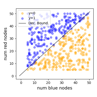
Figure 3: Decision boundary of the linear classifier of DC-SMGNN for RedBlueNodes over the validation split (random seed 1 and 2). The plot is in 2D since RedBlueNodes contains only red or blue nodes.

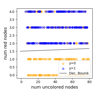
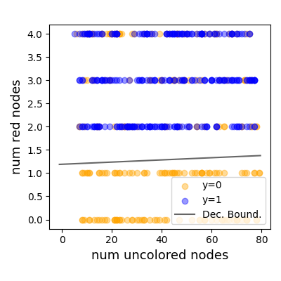
Figure 4: Decision boundary of the linear classifier of DC-SMGNN for TopoFeature over the validation split (random seed 1 and 2). For seed 1, $w_{r}=0.89$, $w_{b}=4e^{-42}$, $w_{u}=-0.001$, and $b=-1.3$. For seed 2, $w_{r}=0.92$, $w_{b}=-1e^{-33}$, $w_{u}=-0.002$, and $b=-1.09$. Since $x_{b}$ equals $0$ as there are no blue nodes in the dataset, we drop its visualization collapsing the plot to 2D. When providing the final interpretable formula, we drop $x_{b}$ and $x_{u}$ due to their sensible lower magnitude. More aggressive sparsification can be applied to the training of the linear model to promote an even lower $w_{u}$.

B.4 Training and evaluation.

Every model is trained for the same 10 random splits, and the optimization protocol is fixed across all experiments following previous work (Miao et al., 2022a) and using the Adam optimizer (Kingma & Ba, 2015). Also, for experiments with Dual-Channel GNN, we fix an initial warmup of 20 epochs where the two channels are trained independently to output the ground truth label. After this warmup, only the overall model is trained altogether. The total number of epochs is fixed to $100$ for every dataset except for Graph-SST2 where it is set to $200$.

For experiments on Graph-SST2 we forced the classifier of any SE-GNNs to have a single GNN layer and a final linear layer mapping the graph embedding to the output. The parameters of the classifier are then different from those of the explanation extractor and trained jointly.

When training SMGNN, to avoid gradient cancellation due to relevance scores approaching exact zero, we use a simple heuristic to push the scores higher when their average value in the batch is below $2e^{-9}$. This is implemented by adding back to the loss of the batch the negated mean scaled by $0.1$. This is similar to value clapping used by GISST, but we found it to yield better empirical performances.

B.5 Software and hardware

Our implementation is done using PyTorch 2.4.1 (Paszke et al., 2017) and PyG 2.4.0 (Fey & Lenssen, 2019). Experiments are run on two different Linux machines, with CUDA 12.6 and a single NVIDIA GeForce RTX 4090, or with CUDA 12.0 and a single NVIDIA TITAN V.

Appendix C Additional Experiments

C.1 Ablation study on how to choose $\mathsf{aggr}$

Table 5: Raw channel relevance scores for the experiments in Table˜2. The "Channel" column reports, the relative importance computed for each channel, For binary classification tasks, the first entry corresponds to the SE-GNN channel, whereas the last is to the interpretable model. For multi-class tasks, the first $|Y|$ entries correspond to the importance for each of the $|Y|$ SE-GNNs outputs, whereas the last $|Y|$ to that of the linear model. For GOODMotif, in particular, $|Y|=3$.

Model	RedBlueNodes		TopoFeature		GOODMotif
	Acc	Channel	Acc	Channel	Acc	Channel
DC-GSAT	100 $\pm$ 00	$[0.02,0.98]\pm 0.05$	100 $\pm$ 00	$[0.47,0.53]\pm 0.27$	93 $\pm$ 01	$[0.33,0.36,0.30,4e^{-3},2e^{-4},1e^{-4}]$ $\pm[0.33,0.36,0.29,1e^{-2},2e^{-4},1e^{-4}]$
DC-SMGNN	100 $\pm$ 00	$[0.05,0.95]\pm 0.10$	100 $\pm$ 00	$[0,31,0,69]\pm 0.11$	93 $\pm$ 00	$[0.27,0.19,0.53,1e^{-4},3e^{-5},1e^{-3}]$ $\pm[0.39,0.29,0.39,0.0,0.0,0.0]$

Table 6: Ablation study for the choice of $\mathsf{aggr}$. The reference architecture in use is SMGNN and the dataset used for the evaluation is TopoFeature. The "Channel" column reports, when $\mathsf{aggr}$ supports it, the relative importance computed for each channel, where the first entry corresponds to the SE-GNN channel, whereas the last to the interpretable model.

$\mathsf{aggr}$	TopoFeature
	Acc	Channel	Num red nodes $\geq$
$\mathsf{aggr}_{\text{G{\"{o}}del}}$	96 $\pm$ 03	Not supported	-
$\mathsf{aggr}_{\text{Product}}$	96 $\pm$ 04	Not supported	-
$\mathsf{aggr}_{\text{Linear}}$	79 $\pm$ 11	$[-1.22,1.77]\pm[1.65,0.92]$	$0.24\pm 1.01$
$\mathsf{aggr}_{\text{MLP}}$	99 $\pm$ 02	Not supported	-
$\mathsf{aggr}_{\text{{LENs}}}$	95 $\pm$ 05	$[0.62,0.38]\pm 0.42$	$0.17\pm 1.47$
$\mathsf{aggr}_{\text{{LENs}}}^{ST}$	65 $\pm$ 07	$[0.01,0.99]\pm 0.01$	$0.70\pm 0.96$
$\mathsf{aggr}_{\text{{(B)LENs}}}$ (ours)	100 $\pm$ 00	$[0.31,0.69]\pm 0.11$	$1.23\pm 0.17$

Our implementation of $\mathsf{aggr}$ relies on LENs to combine the two channels in an interpretable manner. LENs are however found to be susceptible to leakage (Azzolin et al., 2022), that is they can exploit information beyond those encoded in the activated class. Leakage hinders the semantics of input activations, thus comprising the interpretability of the prediction (Margeloiu et al., 2021; Havasi et al., 2022). Popular remedies include binarizing the input activations (Margeloiu et al., 2021; Azzolin et al., 2022; Giannini et al., 2024) so as to force the hidden layers of LENs to focus on the activations themselves, rather than their confidence.

In our work, we adopt a different strategy to avoid leakage in LENs and propose to anneal the temperature of the input activations so as to gradually approach a binary activation during training, while ensuring a smooth differentiation. Input activations are generally assumed to be continuous in $[0,1]$, and usually generated by a sigmoid activation function (Barbiero et al., 2022). Therefore, our temperature annealing simply scales the raw activation before the sigmoid activation by a temperature parameter $\tau$, where $\tau$ is linearly annealed from a value of $1$ to $0.3$. The resulting model is indicated with the name of (Binary)LENs– (B)LENs in short.

In the following ablation study, we investigate different approaches for implementing $\mathsf{aggr}$, showing that only (B)LENs reliably achieve satisfactory performances while preserving the semantics of each channel. The baselines for implementing $\mathsf{aggr}$ considered in our study are as follows:

• Logic combination based on T-norm fuzzy logics, like Gödel $\mathsf{aggr}_{\text{G{\"{o}}del}}(A,B)=min(A,B)$ and Product logic $\mathsf{aggr}_{\text{Product}}(A,B)=A*B$ (Klement et al., 2013).

• Linear combination $\mathsf{aggr}_{\text{Linear}}(A,B)=W[A||B]$, where $||$ concatenates the two inputs.

• Multi-Layer Perceptron $\mathsf{aggr}_{\text{MLP}}(A,B)=W_{3}(\sigma(W_{2}(\sigma W_{1}[A||B])))$.

• Logic Explained Network (LENs) $\mathsf{aggr}_{\text{{LENs}}}(A,B)=\text{{LENs}}(A||B)$.

• Logic Explained Network (LENs) with discrete input $\mathsf{aggr}_{\text{{LENs}}}^{ST}(A,B)=\text{{LENs}}(ST(A)||ST(B))$. The discreteness of the input activations is obtained using the Straight-Trough (ST) reparametrization (Jang et al., 2016; Azzolin et al., 2022; Giannini et al., 2024), which uses the hard discrete scores in the forward step of the network, while relying on their soft continuous version for backpropagation.

We provide in Table˜6 the results for DC-SMGNN using different $\mathsf{aggr}$ choices over TopoFeature. In this dataset, the expected rule to be learned by the interpretable channel is number of red nodes $\geq$ 2. Among the alternatives, $\mathsf{aggr}_{\text{G{\"{o}}del}}$, $\mathsf{aggr}_{\text{Product}}$, and $\mathsf{aggr}_{\text{MLP}}$ do not allow to understand how the channels are combined, resulting in unsuitable $\mathsf{aggr}$ functions for our purpose. $\mathsf{aggr}_{\text{Linear}}$ and $\mathsf{aggr}_{\text{{LENs}}}^{ST}$, instead, fail in solving the task. $\mathsf{aggr}_{\text{{LENs}}}$, however, achieve both a satisfactory accuracy and an interpretable combination of channels. Nonetheless, the presence of leakage hinders a full understanding of the interpretable rule, as the hidden layers of the LENs are allowed to exploit the confidence of the interpretable channel’s predictions in building an alternative rule, that it is now no longer intelligible. Overall, (B)LENs is the only choice that allows the combination of both accuracy and an interpretable combination of the two channels, all while preserving the semantics of the channels as testified by the rule number of red nodes $\geq 1.23$ matching the expectations.

C.2 More experiments on AIDS

In Table˜3 we showed that a simple linear classifier on sum-aggregated node features can suffice for achieving the same, or better, performances than a plain SE-GNN. Even if the linear classifier is promoted for sparsity via weight decay regularization, the resulting model is still difficult to be interpreted, as it assigns non-negligible scores to a multiple of input features, making it difficult to extract a simple rule. For this reason, we extend the original set of node features by concatenating the value $1.0$ for each node. The role of this additional feature is to allow the linear classifier to easily access the graph-level feature number of nodes. We name the resulting updated dataset AIDSC1.

Then, we train the same models as Table˜3, where we increase the sparsity regularization on both the SE-GNN and the linear model, to heavily promote sparsity. This is achieved by setting to $0.1$ the weight decay regularization for the SE-GNN, and to $0.01$ a $L_{1}$ sparsification to the linear classifier. The results are shown in Table˜7, and show that under this strong regularization, SE-GNN struggles to solve the task. Conversely, the Dual-Channel GNN augmentation still solves the task, while providing intelligible predictions. In fact, by inspecting the weights of the linear classifier when picked by the Dual-Channel GNN, the resulting model weights reveal that the model is mainly relying on the count of nodes in the graph, as pointed out in Pluska et al. (2024). For completeness, we report in Table˜9 the full weight matrix for DC-SMGNN.

Table 7: Dual-Channel GNNs solve AIDSC1 even when prompted for strong sparsification, whereas plain SE-GNN achieves suboptimal predictions. Results are averaged only over seeds where the Dual-Channel GNN selects the linear classifier as the main channel. We indicate with superscript numbers the seeds left out from the analysis. The rule is extracted from the last column of Table˜9 and averaged across nine seeds.

Model	AIDSC1
	F1	Channel	Rule
GIN	85 $\pm$ 05	-	-
GISST	68 $\pm$ 06	-	-
DC-GISST 2	99 $\pm$ 02	$\mathsf{Rule}$	num nodes $\leq 12.66\pm 0.18$
GSAT	70 $\pm$ 06	-	-
DC-GSAT 4,10	99 $\pm$ 02	$\mathsf{Rule}$	num nodes $\leq 13.64\pm 1.41$
SMGNN	68 $\pm$ 06	-	-
DC-SMGNN 10	99 $\pm$ 02	$\mathsf{Rule}$	num nodes $\leq 13.89\pm 3.07$

C.3 Dual-Channel GNN can improve the faithfulness of SE-GNNs

To measure the impact of the Dual-Channel GNN augmentation to plain SE-GNNs on the faithfulness of explanations, we compute $\mathsf{Faith}$ (Definition˜5.1) for SMGNN and GSAT with their respective augmentations on TopoFeature and GOODMotif. Following Christiansen et al. (2023), we compute $\mathsf{Faith}$ for both the actual explanation and a randomized explanation obtained by randomly shuffling the explanation scores before feeding them to the classifier, and computing their ratio.

$$\text{$\mathsf{Faith}$ ratio}=\frac{\mathsf{Faith}(\mathcal{E})}{\mathsf{Faith}(R)}$$ (25)

where $R$ is the original explanation, and $\mathcal{E}$ a randomly shuffled explanation. The metric achieves a score of $1$ when the two values match, meaning the model is as faithful to the original explanation as a random explanation, whilst achieves a score of $0$ when the faithfulness of the original explanation is considerably higher than that of a random one.

We compute the metric over the entire validation splits, and extract hard explanations by applying a topK strategy as indicated in previous studies (Amara et al., 2022; Longa et al., 2024), where $k\in[0.3,0.6,0.9]$ for GOODMotif, and $k\in[0.05,0.1,0.2,0.4,0.8]$ for TopoFeature. Perturbations are limited to edge removals, and we force isolated nodes to be removed from the explanation. To compute $\mathsf{Suf}$ and $\mathsf{Nec}$, we refer to the implementation of Azzolin et al. (2024) which requires a hyperparameter $b$ encoding the number of removals to apply at each perturbation. To obtain more robust results, we vary $b\in[0.01,0.05,0.1]$, corresponding to a number of perturbations equal to a $b$ percentage of the graph size. Then, the final $\mathsf{Faith}$ score is taken as the best $\mathsf{Faith}$ across $k$ and averaged across the values of $b$.

The final results are reported in Table˜8 and highlight that for TopoFeature, where both DC-GNNs can exploit the interpretable channel (see Table˜2), Dual-Channel GNNs can achieve considerable gains in faithfulness. DC-GSAT, in particular, achieves a better score but with a considerably higher standard deviation. By inspecting the raw scores, however, we see that across the values $b$, DC-GSAT scores $[1.00,0.05,0.12]$ whereas GSAT achieves $[0.50,0.27,0.48]$, indicating that $b=0.01$ can be an unfortunate choice for this model as it may not bring enough perturbations to let the model change prediction. On the other values of $b$, however, the model achieves a significant gain in faithfulness ratio of almost an order of magnitude. On GOODMotif, instead, as the Dual-Channel GNNs does not have any advantage in using an interpretable model, we do not expect significant changes in the faithfulness scores as indicated in Table˜8, where the only gain is due to higher variance.

We argue that the substantial gains in faithfulness mainly come from the ability of Dual-Channel GNNs to delegate each sub-task to the channel that can best handle it, i.e., learning the motif for the SE-GNN and the "$\geq$" rule to the linear classifier. In doing so, the underlying SE-GNN can better focus on highlighting the topological explanation, resulting in a more faithful explanation. This insight is supported by the analysis of the compactness of explanations provided in Section˜C.4, showing that indeed those SE-GNNs can better focus on the topological sub-task.

Table 8: Faithfulness of SE-GNNs and their augmentations for TopoFeature and GOODMotif. Following (Christiansen et al., 2023), we report the ratio between $\mathsf{Faith}$ computed over randomly shuffled explanations and original ones. Therefore, scores close to zero indicate better values.

Model	TopoFeature	GOODMotif
	$\mathsf{Faith}$ ratio ($\downarrow$)	$\mathsf{Faith}$ ratio ($\downarrow$)
GSAT	0.42 $\pm$ 0.10	0.78 $\pm$ 0.08
DC-GSAT	0.39 $\pm$ 0.43	0.69 $\pm$ 0.11
SMGNN	0.65 $\pm$ 0.28	1.00 $\pm$ 0.00
DC-SMGNN	0.04 $\pm$ 0.04	1.00 $\pm$ 0.00

C.4 Plotting Explanations

In this section, we aim to provide examples of explanations of SE-GNNs and DC-GNNs. For visualization purposes, we rely on an importance threshold to plot the hard explanatory subgraph over the entire graph. Such threshold is picked by plotting the histogram of importance scores and chosen in such a way as to separate regions of higher scores from regions of lower scores. We will analyze the following datasets:

TopoFeature.

Fig.˜5 and Fig.˜6 present the histograms of explanation relevance scores for GSAT and SMGNN respectively. Overall, SMGNN achieves a better separation between higher and lower explanation scores, making it easier to select a proper threshold to plot explanations. Therefore, we will proceed to show explanation examples in Fig.˜7 only for SMGNN for seed 1, picking as threshold the value $0.8$. Overall, the model succeeded in giving considerably higher relevance to edges in the motif, but failed in highlighting red nodes as relevant for predictions of class $1$, hindering a full understanding of the model’s decision process.

We proceed now to analyze the explanations extracted for the same samples for DC-SMGNN. First, we plot the histogram of explanation scores in Fig.˜8, showing better sparsification than a plain SMGNN. For reference, we also plot the histogram for DC-GSAT scores in Fig.˜9, where the same sparsification effect can be observed. Then, we report in Fig.˜10 the explanations for the same graphs as in Fig.˜7, showing that DC-SMGNN achieves better sparsification than a plain SMGNN. In fact, since the rule at least two red nodes is learned by the interpretable model, the underlying SMGNN now just looks at the topological motif, and indeed the substantially more sparse edge score reflects this behavior. Overall, DC-SMGNN explanations reflect more closely the actual predictive behavior of the underlying SE-GNN.

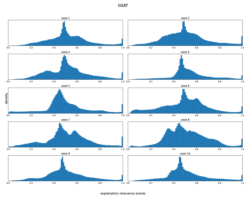
Figure 5: Histograms of explanation relevance scores for GSAT on TopoFeature (validation set). The model fails to reliably separate between relevant and non-relevant edges, making it difficult to select a proper relevance threshold.

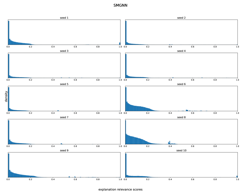
Figure 6: Histograms of explanation relevance scores for SMGNN on TopoFeature (validation set). The sparsification mechanism of SMGNN better separates edges with higher importance than the rest of the graph.

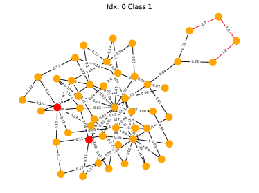
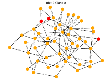
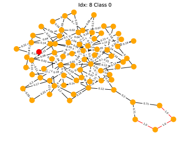
Figure 7: Examples of explanations for SMGNN (seed $1$) over TopoFeature. Relevant edges are those with $p_{uv}\geq 0.8$ and are highlighted in red. Edges are annotated with their respective $p_{uv}$ score. Samples of class $1$ must have both a cycle and at least $2$ red nodes.

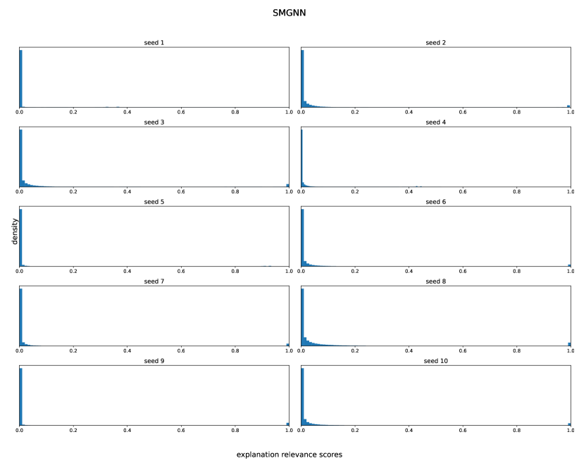
Figure 8: Histograms of explanation relevance scores for DC-SMGNN on TopoFeature (validation set). Since the underlying SMGNN is now only looking for the topological motif (as the rule at least two red nodes is learned by the interpretable model), the Dual-Channel GNN is allowed to sparsify all the other edges better, achieving more compact explanations. For seed $1$, non-zero scores are clutter around $0.38$.

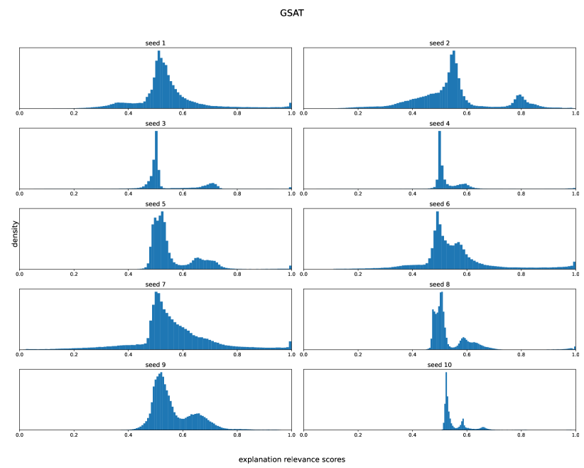
Figure 9: Histograms of explanation relevance scores for DC-GSAT on TopoFeature (validation set).

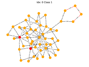
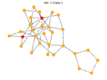
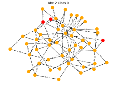
Figure 10: Examples of explanations for DC-SMGNN (seed $1$) over TopoFeature. Relevant edges are those with $p_{uv}\geq 0.2$ and are highlighted in red. The threshold is picked by looking at the histogram in Fig.˜8. Edges are annotated with their respective $p_{uv}$ score. Overall, DC-SMGNN achieves better sparsification than SMGNN (Fig.˜7).

RedBlueNodes.

Fig.˜11 and Fig.˜12 show the edge relevance scores for GSAT and SMGNN respectively. Overall, the histograms show that both models fail to reliably identify a relevant subgraph with a consistently higher importance than irrelevant ones. Examples of explanations for both models, plotted in Fig.˜13 and Fig.˜14, confirm that subgraph-based explanations fail to convey actionable insights into what the model is predicting, as no clear pattern emerges from explanations. Conversely, both DC-GSAT and DC-SMGNN provide intelligible prediction by relying on a simple linear classifier encoding the ground truth rule number of red nodes $\geq$ blue nodes (see Table˜2 and Fig.˜3).

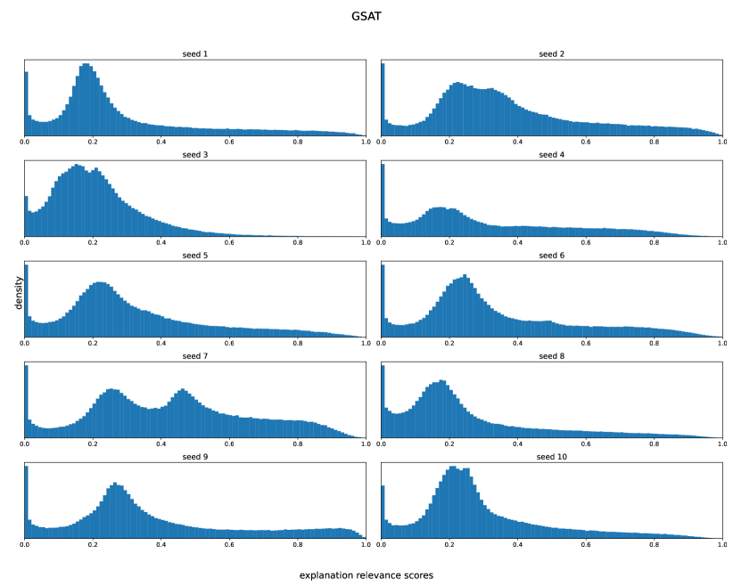
Figure 11: Histograms of explanation relevance scores for GSAT on RedBlueNodes (validation set). The model fails to reliably separate between relevant and non-relevant edges, making it difficult to select a proper relevance threshold. Specifically, most edges are assigned an importance close to $0.3$, which matches the uninformative prior $r$ selected during training.

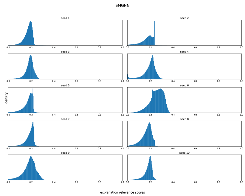
Figure 12: Histograms of explanation relevance scores for SMGNN on RedBlueNodes ((validation set)). The model assigns very cluttered scores to almost all edges, failing to highlight a subset that is reliably more relevant than the others, making it difficult to select an appropriate threshold for showing the explanations to consumers.

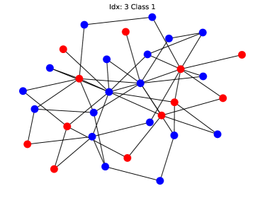
Figure 13: Examples of explanations for GSAT (seed $1$) over RedBlueNodes. Relevant edges are those with $p_{uv}\geq 0.7$ and are highlighted in red. Edges are not annotated with their respective $p_{uv}$ score to avoid excessive clutter.

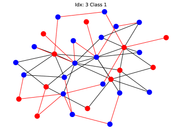
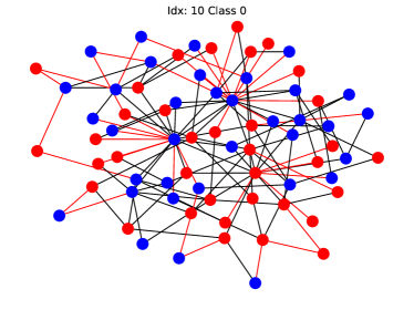
Figure 14: Examples of explanations for SMGNN (seed $1$) over RedBlueNodes. Relevant edges are those with $p_{uv}\geq 0.2$ and are highlighted in red. Edges are not annotated with their respective $p_{uv}$ score to avoid excessive clutter.

AIDS.

Among each random seed, seed $8$ achieves a test F1 score of $1.0$, highlighting that the model is likely to have learned to just count the number of nodes in each graph, and to make the prediction based on such count (Pluska et al., 2024). This strategy is proven to be effective in this dataset, as highlighted in Section˜C.2 and Pluska et al. (2024). By plotting the histogram of explanatory scores in Fig.˜15, and some examples of explanations in Fig.˜16, we cannot unambiguously assess which rule the model is using for making predictions. Conversely, as shown in Section˜C.2, DC-GSAT can achieve the same performances while declaring that only node count statistics are being used for prediction.

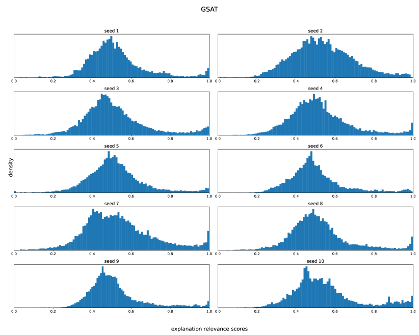
Figure 15: Histograms of explanation relevance scores for GSAT on AIDS (validation set).

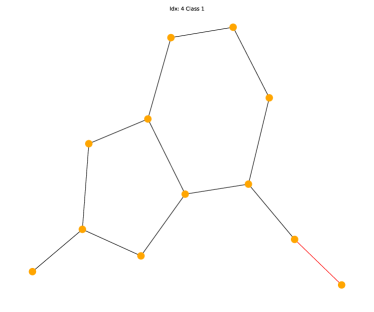
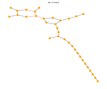
Figure 16: Examples of explanations for GSAT (seed $8$) over AIDS. Relevant edges are those with $p_{uv}\geq 0.8$ and are highlighted in red. Edges are not annotated with their respective $p_{uv}$ score to avoid excessive clutter.

Table 9: Dual-Channel GNN’s linear classifier weights for the DC-SMGNN experiment in Table˜7. The $L_{1}$ sparsification effectively promotes the model to give considerably higher importance to the last input feature, corresponding to the number of nodes in the graph. Seed 10 is omitted as the linear classifier is not in use.

Model	AIDSC1
DC-SMGNN’s seed	Weights (W)	Bias (b)	- b / W[-1]
seed 1	-6.1e-03 -3.2e-02 -9.5e-03 -1.8e-02 -3.8e-04 7.8e-03 -2.4e-04 7.0e-04 5.9e-04 1.4e-03 3.9e-04 1.6e-02 -4.4e-04 1.4e-03 -6.9e-04 4.1e-05 -2.6e-02 -7.0e-04 3.1e-04 -9.6e-04 -3.8e-04 8.9e-04 1.1e-04 3.7e-05 -2.2e-04 -3.3e-04 -3.3e-04 9.7e-04 4.3e-04 1.4e-03 -8.6e-05 3.4e-04 4.1e-04 3.6e-04 1.1e-03 -1.7e-03 1.7e-03 3.4e-04 -2.9e-01	3.64	12.45
seed 2	-2.0e-02 -3.0e-02 8.0e-03 7.3e-03 -7.3e-04 2.7e-02 -6.5e-04 2.0e-02 -4.9e-05 -9.4e-04 7.2e-02 -4.0e-04 -1.4e-04 -2.6e-04 -3.4e-04 1.1e-03 3.0e-04 8.4e-06 1.3e-04 -9.4e-04 -3.9e-05 -9.3e-04 -5.1e-04 -1.4e-03 6.3e-04 3.4e-04 1.3e-03 5.6e-04 1.2e-04 -6.4e-04 4.5e-04 3.8e-05 8.0e-05 1.6e-04 -3.3e-04 1.3e-04 7.1e-04 5.9e-04 -2.9e-01	3.63	12.57
seed 3	-1.2e-02 -3.1e-02 3.2e-04 2.4e-04 3.6e-04 2.4e-03 -1.4e-04 -4.4e-04 1.5e-06 1.8e-05 6.1e-05 2.4e-04 6.5e-04 -1.2e-04 -2.3e-04 -6.4e-04 -3.1e-04 1.0e-03 -2.8e-03 -1.2e-03 -3.9e-05 1.1e-03 -5.2e-04 -6.0e-04 -1.1e-03 -4.1e-05 2.0e-04 -3.6e-04 -9.2e-04 -7.6e-04 -3.4e-05 -1.3e-04 -8.7e-04 -8.2e-04 -1.4e-03 5.4e-04 6.6e-04 -3.3e-04 -2.7e-01	3.38	12.45
seed 4	-9.7e-03 -1.6e-02 -7.9e-03 -2.0e-02 8.0e-04 4.8e-03 -5.9e-04 6.0e-05 3.9e-04 -1.1e-03 -3.6e-04 6.3e-04 -1.7e-03 3.2e-04 -1.0e-03 4.4e-04 -3.4e-02 7.9e-04 -8.5e-04 -6.0e-04 4.7e-04 -2.8e-04 -9.4e-04 -5.9e-04 -1.0e-03 1.2e-05 -7.1e-05 -5.1e-05 9.3e-04 1.3e-03 1.5e-04 -1.3e-04 -4.9e-04 5.1e-04 7.9e-04 2.5e-05 -4.0e-04 -4.4e-04 -2.8e-01	3.42	12.04
seed 5	-1.7e-01 -2.0e-01 -1.3e-01 1.2e-04 -8.6e-04 -1.2e-03 2.1e-04 -2.0e-04 -1.4e-03 -5.7e-04 1.3e-04 -5.2e-04 -3.5e-04 -9.1e-04 4.6e-04 -6.7e-04 3.6e-04 1.0e-03 -6.8e-04 -4.0e-04 -4.7e-04 -9.2e-04 8.1e-04 -5.2e-04 -1.9e-06 -2.4e-04 -5.2e-04 2.0e-04 4.5e-04 -1.3e-03 5.5e-04 2.5e-04 -5.5e-04 6.2e-04 -1.0e-03 4.2e-04 2.1e-04 8.9e-04 -2.0e-01	4.48	22.18
seed 6	-1.0e-02 -6.9e-02 -2.0e-03 -1.3e-02 -4.7e-03 1.5e-02 -1.1e-03 5.1e-04 8.4e-04 7.4e-04 -8.2e-04 -3.4e-04 -1.3e-03 6.7e-04 -8.1e-07 1.3e-03 -1.7e-02 6.9e-04 2.7e-04 8.7e-04 -8.5e-05 3.1e-04 -3.1e-04 -5.3e-04 -9.0e-04 -4.1e-04 1.2e-03 5.8e-04 -4.2e-04 1.6e-03 -5.1e-04 9.4e-04 4.4e-04 8.4e-04 6.4e-05 2.4e-04 -1.7e-04 -9.2e-04 -2.6e-01	3.90	15.07
seed 7	-1.8e-02 -2.7e-02 -5.5e-03 -1.6e-02 4.9e-04 -4.3e-03 -8.5e-04 1.6e-04 -8.3e-04 9.1e-04 -5.5e-04 -1.1e-03 -6.8e-04 -1.6e-04 -1.4e-03 9.0e-04 -3.5e-02 2.6e-04 1.3e-03 3.0e-04 -5.3e-05 -1.0e-03 -1.0e-03 -4.5e-04 7.9e-04 6.3e-04 1.3e-03 -5.1e-04 8.9e-04 -4.7e-04 2.0e-03 1.0e-03 -3.9e-04 -1.0e-03 -1.0e-04 4.6e-04 1.0e-03 -6.5e-04 -2.9e-01	3.63	12.32
seed 8	-1.0e-02 -2.2e-02 2.0e-03 -1.6e-02 3.1e-04 5.0e-04 -1.2e-03 -3.9e-04 7.8e-04 -5.8e-04 9.9e-05 -8.4e-04 7.6e-04 -3.9e-04 2.0e-04 7.2e-04 -2.3e-02 -5.3e-04 -4.5e-04 7.0e-04 5.9e-04 -1.1e-04 6.5e-04 -6.3e-04 7.9e-06 -5.8e-04 -3.3e-04 -5.5e-04 -1.2e-03 -9.8e-05 -7.0e-05 3.1e-04 -3.4e-04 -2.0e-03 7.8e-05 -3.5e-04 -8.5e-04 3.3e-05 -2.9e-01	3.47	12.18
seed 9	-1.4e-02 -3.1e-02 5.7e-03 -2.1e-02 -2.2e-04 8.5e-03 3.0e-05 1.3e-04 -6.1e-04 5.7e-04 1.2e-04 -2.5e-03 -1.3e-03 -1.8e-04 1.7e-03 2.5e-04 -2.7e-02 6.9e-04 2.5e-04 1.1e-03 -5.1e-04 -9.9e-04 1.5e-04 1.1e-04 2.4e-04 -9.5e-04 -8.2e-04 1.6e-04 -3.8e-04 -6.3e-04 -5.5e-04 1.7e-03 1.0e-03 -1.1e-04 6.4e-04 7.1e-04 -1.9e-04 -4.5e-04 -2.6e-01	3.59	13.73

References

- Agarwal et al. (2023) Agarwal, C., Queen, O., Lakkaraju, H., and Zitnik, M. Evaluating explainability for graph neural networks. Scientific Data, 10(1):144, 2023.
- Agarwal et al. (2024) Agarwal, C., Tanneru, S. H., and Lakkaraju, H. Faithfulness vs. plausibility: On the (un)reliability of explanations from large language models, 2024.
- Amara et al. (2022) Amara, K., Ying, Z., Zhang, Z., Han, Z., Zhao, Y., Shan, Y., Brandes, U., Schemm, S., and Zhang, C. Graphframex: Towards systematic evaluation of explainability methods for graph neural networks. In Learning on Graphs Conference, pp. 44–1. PMLR, 2022.
- Azzolin et al. (2022) Azzolin, S., Longa, A., Barbiero, P., Lio, P., and Passerini, A. Global explainability of gnns via logic combination of learned concepts. In The Eleventh International Conference on Learning Representations, 2022.
- Azzolin et al. (2024) Azzolin, S., Longa, A., Teso, S., and Passerini, A. Perks and pitfalls of faithfulness in regular, self-explainable and domain invariant gnns, 2024. URL https://arxiv.org/abs/2406.15156.
- Barabási & Albert (1999) Barabási, A.-L. and Albert, R. Emergence of scaling in random networks. science, 286(5439):509–512, 1999.
- Barbiero et al. (2022) Barbiero, P., Ciravegna, G., Giannini, F., Lió, P., Gori, M., and Melacci, S. Entropy-based logic explanations of neural networks. In Proceedings of the AAAI Conference on Artificial Intelligence, volume 36, pp. 6046–6054, 2022.
- Barceló et al. (2020) Barceló, P., Kostylev, E. V., Monet, M., Pérez, J., Reutter, J., and Silva, J.-P. The logical expressiveness of graph neural networks. In ICLR, 2020.
- Bechler-Speicher et al. (2023) Bechler-Speicher, M., Amos, I., Gilad-Bachrach, R., and Globerson, A. Graph neural networks use graphs when they shouldn’t. arXiv preprint arXiv:2309.04332, 2023.
- Bechler-Speicher et al. (2024) Bechler-Speicher, M., Globerson, A., and Gilad-Bachrach, R. The intelligible and effective graph neural additive network. In The Thirty-eighth Annual Conference on Neural Information Processing Systems, 2024. URL https://openreview.net/forum?id=SKY1ScUTwA.
- Beckers (2022) Beckers, S. Causal Explanations and XAI. In Conference on Causal Learning and Reasoning, pp. 90–109, 2022.
- Bhattacharjee & von Luxburg (2024) Bhattacharjee, R. and von Luxburg, U. Auditing local explanations is hard. arXiv preprint arXiv:2407.13281, 2024.
- Chen et al. (2022) Chen, Y., Zhang, Y., Bian, Y., Yang, H., Kaili, M., Xie, B., Liu, T., Han, B., and Cheng, J. Learning causally invariant representations for out-of-distribution generalization on graphs. Advances in Neural Information Processing Systems, 35:22131–22148, 2022.
- Chen et al. (2024) Chen, Y., Bian, Y., Han, B., and Cheng, J. How interpretable are interpretable graph neural networks? In Forty-first International Conference on Machine Learning, 2024.
- Christiansen et al. (2023) Christiansen, M., Villadsen, L., Zhong, Z., Teso, S., and Mottin, D. How faithful are self-explainable gnns? arXiv preprint arXiv:2308.15096, 2023.
- Dai & Wang (2021) Dai, E. and Wang, S. Towards self-explainable graph neural network. In Proceedings of the 30th ACM International Conference on Information & Knowledge Management, pp. 302–311, 2021.
- Dai & Wang (2022) Dai, E. and Wang, S. Towards prototype-based self-explainable graph neural network. arXiv preprint arXiv:2210.01974, 2022.
- Darwiche & Hirth (2023) Darwiche, A. and Hirth, A. On the (complete) reasons behind decisions. Journal of Logic, Language and Information, 32(1):63–88, 2023.
- Debnath et al. (1991) Debnath, A. K., Lopez de Compadre, R. L., Debnath, G., Shusterman, A. J., and Hansch, C. Structure-activity relationship of mutagenic aromatic and heteroaromatic nitro compounds. correlation with molecular orbital energies and hydrophobicity. Journal of medicinal chemistry, 34(2):786–797, 1991.
- Deng & Shen (2024) Deng, J. and Shen, Y. Self-interpretable graph learning with sufficient and necessary explanations. In Proceedings of the AAAI Conference on Artificial Intelligence, volume 38, pp. 11749–11756, 2024.
- Erdos et al. (1959) Erdos, P., Rényi, A., et al. On random graphs i. Publ. math. debrecen, 6(290-297):18, 1959.
- Ferrini et al. (2024) Ferrini, F., Longa, A., Passerini, A., and Jaeger, M. A self-explainable heterogeneous gnn for relational deep learning. arXiv preprint arXiv:2412.00521, 2024.
- Fey & Lenssen (2019) Fey, M. and Lenssen, J. E. Fast graph representation learning with pytorch geometric. arXiv preprint arXiv:1903.02428, 2019.
- Fontanesi et al. (2024) Fontanesi, M., Micheli, A., and Podda, M. Xai and bias of deep graph networks. ESANN, 2024.
- Giannini et al. (2024) Giannini, F., Fioravanti, S., Keskin, O., Lupidi, A., Magister, L. C., Lió, P., and Barbiero, P. Interpretable graph networks formulate universal algebra conjectures. Advances in Neural Information Processing Systems, 36, 2024.
- Giunchiglia et al. (2022) Giunchiglia, V., Shukla, C. V., Gonzalez, G., and Agarwal, C. Towards training GNNs using explanation directed message passing. In The First Learning on Graphs Conference, 2022. URL https://openreview.net/forum?id=_nlbNbawXDi.
- Gravina et al. (2022) Gravina, A., Bacciu, D., and Gallicchio, C. Anti-symmetric dgn: a stable architecture for deep graph networks. In The Eleventh International Conference on Learning Representations, 2022.
- Grohe (2021) Grohe, M. The logic of graph neural networks. In 36th Annual ACM/IEEE Symposium on Logic in Computer Science (LICS), pp. 1–17, 2021.
- Gui et al. (2022) Gui, S., Li, X., Wang, L., and Ji, S. GOOD: A graph out-of-distribution benchmark. In Thirty-sixth Conference on Neural Information Processing Systems Datasets and Benchmarks Track, 2022. URL https://openreview.net/forum?id=8hHg-zs_p-h.
- Gui et al. (2023) Gui, S., Liu, M., Li, X., Luo, Y., and Ji, S. Joint learning of label and environment causal independence for graph out-of-distribution generalization. arXiv preprint arXiv:2306.01103, 2023.
- Havasi et al. (2022) Havasi, M., Parbhoo, S., and Doshi-Velez, F. Addressing leakage in concept bottleneck models. In Oh, A. H., Agarwal, A., Belgrave, D., and Cho, K. (eds.), Advances in Neural Information Processing Systems, 2022. URL https://openreview.net/forum?id=tglniD_fn9.
- Ignatiev et al. (2015) Ignatiev, A., Previti, A., and Marques-Silva, J. Sat-based formula simplification. In Theory and Applications of Satisfiability Testing – SAT 2015, pp. 287–298. Springer International Publishing, 2015.
- Ignatiev et al. (2019) Ignatiev, A., Narodytska, N., and Marques-Silva, J. On relating explanations and adversarial examples. NeurIPS, 2019.
- Ioffe (2015) Ioffe, S. Batch normalization: Accelerating deep network training by reducing internal covariate shift. arXiv preprint arXiv:1502.03167, 2015.
- Jang et al. (2016) Jang, E., Gu, S., and Poole, B. Categorical reparameterization with gumbel-softmax. arXiv preprint arXiv:1611.01144, 2016.
- Jin et al. (2020) Jin, W., Barzilay, R., and Jaakkola, T. Multi-objective molecule generation using interpretable substructures. In International conference on machine learning, pp. 4849–4859. PMLR, 2020.
- Kingma & Ba (2015) Kingma, D. P. and Ba, J. Adam: A method for stochastic optimization. In International Conference on Learning Representations, 2015.
- Klement et al. (2013) Klement, E. P., Mesiar, R., and Pap, E. Triangular norms, volume 8. Springer Science & Business Media, 2013.
- Knyazev et al. (2019) Knyazev, B., Taylor, G. W., and Amer, M. Understanding attention and generalization in graph neural networks. Advances in neural information processing systems, 32, 2019.
- Köhler & Heindorf (2024) Köhler, D. and Heindorf, S. Utilizing description logics for global explanations of heterogeneous graph neural networks. arXiv preprint arXiv:2405.12654, 2024.
- Kraskov et al. (2004) Kraskov, A., Stögbauer, H., and Grassberger, P. Estimating mutual information. Physical Review E—Statistical, Nonlinear, and Soft Matter Physics, 69(6):066138, 2004.
- Li et al. (2024) Li, Z., Geisler, S., Wang, Y., Günnemann, S., and van Leeuwen, M. Explainable graph neural networks under fire, 2024. URL https://arxiv.org/abs/2406.06417.
- Lin et al. (2020) Lin, C., Sun, G. J., Bulusu, K. C., Dry, J. R., and Hernandez, M. Graph neural networks including sparse interpretability. arXiv preprint arXiv:2007.00119, 2020.
- Longa et al. (2024) Longa, A., Azzolin, S., Santin, G., Cencetti, G., Liò, P., Lepri, B., and Passerini, A. Explaining the explainers in graph neural networks: a comparative study. ACM Computing Surveys, 2024.
- Luo et al. (2020) Luo, D., Cheng, W., Xu, D., Yu, W., Zong, B., Chen, H., and Zhang, X. Parameterized explainer for graph neural network. Advances in neural information processing systems, 33:19620–19631, 2020.
- Margeloiu et al. (2021) Margeloiu, A., Ashman, M., Bhatt, U., Chen, Y., Jamnik, M., and Weller, A. Do concept bottleneck models learn as intended? arXiv preprint arXiv:2105.04289, 2021.
- Marques-Silva (2023) Marques-Silva, J. Logic-based explainability in machine learning. In Reasoning Web. Causality, Explanations and Declarative Knowledge: 18th International Summer School 2022, Berlin, Germany, September 27–30, 2022, Tutorial Lectures, pp. 24–104. Springer, 2023.
- Marques-Silva & Ignatiev (2022) Marques-Silva, J. and Ignatiev, A. Delivering trustworthy ai through formal xai. In Proceedings of the AAAI Conference on Artificial Intelligence, volume 36, pp. 12342–12350, 2022.
- Marques-Silva et al. (2020) Marques-Silva, J., Gerspacher, T., Cooper, M. C., Ignatiev, A., and Narodytska, N. Explaining naive bayes and other linear classifiers with polynomial time and delay. In Proceedings of the 34th International Conference on Neural Information Processing Systems, NIPS ’20, 2020. ISBN 9781713829546.
- Martins et al. (2012) Martins, I. F., Teixeira, A. L., Pinheiro, L., and Falcao, A. O. A bayesian approach to in silico blood-brain barrier penetration modeling. Journal of chemical information and modeling, 52(6):1686–1697, 2012.
- McAllester & Stratos (2020) McAllester, D. and Stratos, K. Formal limitations on the measurement of mutual information. In International Conference on Artificial Intelligence and Statistics, pp. 875–884. PMLR, 2020.
- Miao et al. (2022a) Miao, S., Liu, M., and Li, P. Interpretable and generalizable graph learning via stochastic attention mechanism. In International Conference on Machine Learning, pp. 15524–15543. PMLR, 2022a.
- Miao et al. (2022b) Miao, S., Luo, Y., Liu, M., and Li, P. Interpretable geometric deep learning via learnable randomness injection. In The Eleventh International Conference on Learning Representations, 2022b.
- Morris et al. (2020) Morris, C., Kriege, N. M., Bause, F., Kersting, K., Mutzel, P., and Neumann, M. Tudataset: A collection of benchmark datasets for learning with graphs. arXiv preprint arXiv:2007.08663, 2020.
- Müller et al. (2023) Müller, P., Faber, L., Martinkus, K., and Wattenhofer, R. Graphchef: Learning the recipe of your dataset. In ICML 3rd Workshop on Interpretable Machine Learning in Healthcare (IMLH), 2023. URL https://openreview.net/forum?id=ZgYZH5PFEg.
- Paszke et al. (2017) Paszke, A., Gross, S., Chintala, S., Chanan, G., Yang, E., DeVito, Z., Lin, Z., Desmaison, A., Antiga, L., and Lerer, A. Automatic differentiation in pytorch. In NIPS-W, 2017.
- Pluska et al. (2024) Pluska, A., Welke, P., Gärtner, T., and Malhotra, S. Logical distillation of graph neural networks. In ICML 2024 Workshop on Mechanistic Interpretability, 2024.
- Ragno et al. (2022) Ragno, A., La Rosa, B., and Capobianco, R. Prototype-based interpretable graph neural networks. IEEE Transactions on Artificial Intelligence, 2022.
- Riesen & Bunke (2008) Riesen, K. and Bunke, H. Iam graph database repository for graph based pattern recognition and machine learning. In Structural, Syntactic, and Statistical Pattern Recognition: Joint IAPR International Workshop, SSPR & SPR 2008, Orlando, USA, December 4-6, 2008. Proceedings, pp. 287–297. Springer, 2008.
- Rudin (2019) Rudin, C. Stop explaining black box machine learning models for high stakes decisions and use interpretable models instead. Nature Machine Intelligence, 1(5):206–215, 2019.
- Scarselli et al. (2008) Scarselli, F., Gori, M., Tsoi, A. C., Hagenbuchner, M., and Monfardini, G. The graph neural network model. IEEE transactions on neural networks, 20(1):61–80, 2008.
- Serra & Niepert (2022) Serra, G. and Niepert, M. Learning to explain graph neural networks. arXiv preprint arXiv:2209.14402, 2022.
- Setzu et al. (2021) Setzu, M., Guidotti, R., Monreale, A., Turini, F., Pedreschi, D., and Giannotti, F. Glocalx-from local to global explanations of black box ai models. Artificial Intelligence, 294:103457, 2021.
- Shih et al. (2018) Shih, A., Choi, A., and Darwiche, A. A symbolic approach to explaining bayesian network classifiers. arXiv preprint arXiv:1805.03364, 2018.
- Sundararajan et al. (2017) Sundararajan, M., Taly, A., and Yan, Q. Axiomatic attribution for deep networks. In International conference on machine learning, pp. 3319–3328. PMLR, 2017.
- Sushko et al. (2012) Sushko, I., Salmina, E., Potemkin, V. A., Poda, G., and Tetko, I. V. Toxalerts: A web server of structural alerts for toxic chemicals and compounds with potential adverse reactions. Journal of Chemical Information and Modeling, 52(8):2310–2316, 2012. doi: 10.1021/ci300245q.
- Tan et al. (2022) Tan, J., Geng, S., Fu, Z., Ge, Y., Xu, S., Li, Y., and Zhang, Y. Learning and evaluating graph neural network explanations based on counterfactual and factual reasoning. In Proceedings of the ACM Web Conference 2022, WWW ’22, pp. 1018–1027, New York, NY, USA, 2022. Association for Computing Machinery. ISBN 9781450390965. doi: 10.1145/3485447.3511948. URL https://doi.org/10.1145/3485447.3511948.
- Teso et al. (2023) Teso, S., Alkan, Ö., Stammer, W., and Daly, E. Leveraging explanations in interactive machine learning: An overview. Frontiers in Artificial Intelligence, 2023.
- Tishby et al. (2000) Tishby, N., Pereira, F. C., and Bialek, W. The information bottleneck method. ArXiv, physics/0004057, 2000. URL https://api.semanticscholar.org/CorpusID:8936496.
- Wang et al. (2021) Wang, E., Khosravi, P., and Van den Broeck, G. Probabilistic sufficient explanations. 2021.
- Weisstein (2025) Weisstein, E. W. Edge cover, 2025. URL https://mathworld.wolfram.com/EdgeCover.html.
- Wong et al. (2024) Wong, F., Zheng, E. J., Valeri, J. A., Donghia, N. M., Anahtar, M. N., Omori, S., Li, A., Cubillos-Ruiz, A., Krishnan, A., Jin, W., et al. Discovery of a structural class of antibiotics with explainable deep learning. Nature, 626(7997):177–185, 2024.
- Wu et al. (2020a) Wu, T., Ren, H., Li, P., and Leskovec, J. Graph information bottleneck. Advances in Neural Information Processing Systems, 33:20437–20448, 2020a.
- Wu et al. (2022) Wu, Y.-X., Wang, X., Zhang, A., He, X., and Chua, T.-S. Discovering invariant rationales for graph neural networks. arXiv preprint arXiv:2201.12872, 2022.
- Wu et al. (2018) Wu, Z., Ramsundar, B., Feinberg, E. N., Gomes, J., Geniesse, C., Pappu, A. S., Leswing, K., and Pande, V. Moleculenet: a benchmark for molecular machine learning. Chemical science, 9(2):513–530, 2018.
- Wu et al. (2020b) Wu, Z., Pan, S., Chen, F., Long, G., Zhang, C., and Philip, S. Y. A comprehensive survey on graph neural networks. IEEE transactions on neural networks and learning systems, 2020b.
- Xu et al. (2018) Xu, K., Hu, W., Leskovec, J., and Jegelka, S. How powerful are graph neural networks? arXiv preprint arXiv:1810.00826, 2018.
- Ying et al. (2019) Ying, Z., Bourgeois, D., You, J., Zitnik, M., and Leskovec, J. Gnnexplainer: Generating explanations for graph neural networks. Advances in neural information processing systems, 32, 2019.
- Yu et al. (2020) Yu, J., Xu, T., Rong, Y., Bian, Y., Huang, J., and He, R. Graph information bottleneck for subgraph recognition. In International Conference on Learning Representations, 2020.
- Yu et al. (2022) Yu, J., Cao, J., and He, R. Improving subgraph recognition with variational graph information bottleneck. In Proceedings of the IEEE/CVF Conference on Computer Vision and Pattern Recognition, pp. 19396–19405, 2022.
- Yu et al. (2023) Yu, J., Ignatiev, A., and Stuckey, P. J. On formal feature attribution and its approximation. arXiv preprint arXiv:2307.03380, 2023.
- Yuan et al. (2021) Yuan, H., Yu, H., Wang, J., Li, K., and Ji, S. On explainability of graph neural networks via subgraph explorations. In International conference on machine learning, pp. 12241–12252. PMLR, 2021.
- Yuan et al. (2022) Yuan, H., Yu, H., Gui, S., and Ji, S. Explainability in graph neural networks: A taxonomic survey. IEEE transactions on pattern analysis and machine intelligence, 45(5):5782–5799, 2022.
- Zhang et al. (2022) Zhang, Z., Liu, Q., Wang, H., Lu, C., and Lee, C. Protgnn: Towards self-explaining graph neural networks. In Proceedings of the AAAI Conference on Artificial Intelligence, volume 36, pp. 9127–9135, 2022.