GNN-DT: Graph Neural Network Enhanced Decision Transformer for Efficient Optimization in Dynamic Environments

Abstract

Reinforcement Learning (RL) methods used for solving real-world optimization problems often involve dynamic state-action spaces, larger scale, and sparse rewards, leading to significant challenges in convergence, scalability, and efficient exploration of the solution space. This study introduces GNN-DT, a novel Decision Transformer (DT) architecture that integrates Graph Neural Network (GNN) embedders with a novel residual connection between input and output tokens crucial for handling dynamic environments. By learning from previously collected trajectories, GNN-DT reduces dependence on accurate simulators and tackles the sparse rewards limitations of online RL algorithms. We evaluate GNN-DT on the complex electric vehicle (EV) charging optimization problem and prove that its performance is superior and requires significantly fewer training trajectories, thus improving sample efficiency compared to existing DT baselines. Furthermore, GNN-DT exhibits robust generalization to unseen environments and larger action spaces, addressing a critical gap in prior DT-based approaches.

1 Introduction

Sequential decision-making problems are critical for efficiently operating a wide array of industries, such as power systems control (Roald et al., 2023), logistics optimization (Konstantakopoulos et al., 2022), portfolio management (Gunjan & Bhattacharyya, 2023), and advanced manufacturing processes (Gupta & Gupta, 2020). However, many practical problems, such as the electric vehicle (EV) charging optimization (Panda & Tindemans, 2024), are large-scale, have temporal dependencies, and aggregated constraints, often making conventional methods impractical (Bubeck, 2015). This is especially observed in dynamic environments, where the optimization landscape continuously evolves, requiring real-time solutions.

Reinforcement learning (RL) (Sutton & Barto, 2018) has been extensively studied for solving optimization problems due to its ability to manage uncertainty, adapt to dynamic environments, and enhance decision-making through trial-and-error (Lan et al., 2023; Zhang et al., 2023a). In complex and large-scale scenarios, RL can provide high-quality solutions in real-time compared to traditional mathematical programming techniques that fail to do so (Jaimungal, 2022). However, RL approaches face significant challenges, such as sparse reward signals that slow learning and hinder convergence to optimal policies (Dulac-Arnold et al., 2021). In addition, RL solutions struggle to generalize when deployed in environments different from the one they were trained in, limiting their applicability in real-world scenarios with constantly changing conditions (Wang, 2024).

Decision Transformers (DT) (Chen et al., 2021) is an offline RL algorithm that reframes traditional RL problems as generative sequence modeling tasks conditioned on future rewards (Zhang et al., 2023c). By learning from historical data, DTs effectively address the sparse reward issue inherent in online RL, relying on demonstrated successful outcomes instead of extensive trial-and-error exploration. However, the trajectory-stitching mechanism of DT often proves insufficient in dynamic real-world environments, leading to suboptimal policies. Although improved variants such as Q-regularized DT (Q-DT) (Hu et al., 2024) incorporate additional constraints for greater robustness, they still face significant challenges in generalizing across non-stationary tasks (Paster et al., 2024). Consequently, further architectural advances and training strategies are essential to ensure consistent performance in complex environments.

This study introduces GNN-DT, a novel DT architecture that leverages the permutation-equivariant properties of Graph Neural Networks (GNNs) to handle dynamically changing state-action spaces (i.e., varying numbers of nodes over time) and improve generalization. By generating embeddings that remain consistent under node reordering, GNNs offer a powerful way to capture relational information in complex dynamic environments. Moreover, GNN-DT features a novel residual connection between input and output tokens, ensuring that action outputs are informed by the dynamically learned state embeddings for more robust decision-making. To demonstrate the superior performance of the proposed method, we conduct extensive experiments on the complex multi-objective EV charging optimization problem (Orfanoudakis et al., 2024a), which encompasses sparse rewards, temporal dependencies, and aggregated constraints. The main contributions are summarized as follows:

• Introducing a novel DT architecture integrating GNN embeddings, resulting in enhanced sample efficiency, superior performance, robust generalization to unseen environments, and effective scalability to larger action spaces, demonstrating the critical role of GNN-based embeddings in the model’s improvement.

• Demonstrating that online RL algorithms and offline DT baselines, even when trained on diverse datasets (Optimal, Random, Business-as-Usual) with varying sample sizes, perform inferior to GNN-DT when dealing with real-world optimization tasks.

• Proving that both the size and type of training dataset critically influence the learning process of DTs, highlighting the importance of dataset selection.

• Highlighting that strategically integrating high- and low-quality training data (Optimal & Random datasets) significantly enhances policy learning, outperforming models trained exclusively on single-policy datasets.

2 Related Work

Advancements in Decision Transformers

Classic DT encounters significant challenges, including limited trajectory stitching capabilities and difficulties in adapting to online environments. To address these issues, several enhancements have been proposed. The Q-DT (Hu et al., 2024) improves the ability to derive optimal policies from sub-optimal trajectories by relabeling return-to-go values in the training data. Elastic DT (Wu et al., 2024) enhances classic DT by enabling trajectory stitching during action inference at test time, while Multi-Game DT (Lee et al., 2024) advances its task generalization capabilities. The Online DT (Zheng et al., 2022; Villarrubia-Martin et al., 2023) extends DTs to online settings by combining offline pretraining with online fine-tuning, facilitating continuous policy updates in dynamic environments. Additionally, adaptations for offline safe RL incorporate cost tokens alongside rewards (Liu et al., 2023; Hong et al., 2024). DT has also been effectively applied to real-world domains, such as healthcare (Zhang et al., 2023c) and chip design (Lai et al., 2023), showcasing its versatility and practical utility.

RL for EV Smart Charging

RL algorithms offer notable advantages for EV dispatch, including the ability to handle nonlinear models, robustly quantify uncertainty, and deliver faster computation than traditional mathematical programming (Qiu et al., 2023). Popular methods, such as DDPG (Jin et al., 2022), SAC (Jin & Xu, 2021), and batch RL (Sadeghianpourhamami et al., 2020), show promise but often lack formal constraint satisfaction guarantees and struggle to scale with high-dimensional state-action spaces (Yılmaz et al., 2024; Li et al., 2022). Safe RL frameworks address these drawbacks by imposing constraints via constrained MDPs, but typically sacrifice performance and scalability (Zhang et al., 2023b; Chen & Shi, 2022). Multiagent RL techniques distribute complexity across multiple agents, e.g. charging points, stations, or aggregators (Kamrani et al., 2025), yet still encounter convergence challenges and may underperform in large-scale applications. To the best of our knowledge, no study has used DTs for solving the complex EV charging problem, despite DT’s potential to handle sparse rewards effectively.

3 Preliminaries

In this section, an introduction to offline RL and the mathematical formulation of the EV charging optimization problem is presented as an example of what type of problems can be solved by the proposed GNN-DT methodology.

3.1 Offline RL

Offline RL aims to learn a policy $\pi_{\theta}(a\!\mid\!s)$ that maximizes the expected discounted return $\mathbb{E}\bigl{[}\sum_{t=0}^{\infty}\gamma^{t}R(s_{t},a_{t})\bigr{]}$ without additional interactions with the environment (Levine et al., 2020). A Markov Decision Process (MDP) is defined by the tuple $(S,A,P,R,\gamma)$, where $S$ is the state space, $A$ the action space, $P$ the transition function, $R$ the reward function, $\gamma\in(0,1]$ the discount factor (Sutton & Barto, 2018). In the offline setting, a static dataset $\mathcal{D}=\{(s,a,r)\}$, collected by a (potentially suboptimal) policy, is provided. DTs leverage this dataset by treating RL trajectories as sequences, learning to predict actions that maximize returns based on previously collected experiences. A key component in DTs is the return-to-go (RTG), which for a time step $t$ can be defined as:

$$G_{t}=\sum_{\tau=t}^{T}\gamma^{\tau-t}\,r_{\tau},$$ (1)

representing the discounted cumulative reward from $t$ until the terminal time $T$. This formulation is particularly beneficial when real-time exploration is costly or impractical, while sufficient historical data remain available for training.

3.2 The EV Smart Charging Problem

We consider a set of $\mathcal{I}$ charging stations indexed i, all assumed to be controlled by a charge point operator (CPO) over a time window $\mathcal{T}$, divided into $T$ non-overlapping length intervals $\Delta t>0$. For a given time window, each charging station $i$ operates a set of $\mathcal{J}$ non-overlapping charging sessions, denoted by $\mathcal{J}_{i}=\{j_{i,1},\cdots,j_{i,J_{i}}\}$, where $J_{i,j}$ represents the $j^{th}$ charging event at the $i^{th}$ charging station and $J_{i}=|\mathcal{J}_{i}|$ is the total number of charging sessions seen by charging station i in an episode. A charging session is then represented as $j_{j,c}:\{t^{a}_{j,i},t^{d}_{j,i},\bar{p}_{j,i},e^{*}_{j,i}\},~\forall j,i$, where $t^{a},t^{d},\bar{p}$ and $e^{*}$ represent the arrival time, departure time, maximum charging power, and the desired battery energy level at the departure time. The primary goal is to minimize the total energy cost given by:

$$f_{1}(p^{+},p^{-})=\sum_{t\in\mathcal{T}}\sum_{i\in\mathcal{I}}\Delta t(\Pi^{+}_{t}p_{i,t}^{+}-\Pi^{-}_{t}p_{i,t}^{-})$$ (2)

$p^{+}_{i,t}$ and $p^{-}_{i,t}$ denote the charging or discharging power of the $i^{th}$ charging station during time interval $t$. $\Pi^{+}_{t}$ and $\Pi^{-}_{t}$ are the charging and discharging costs, respectively. Along with minimizing the total energy costs , the CPO also wants the aggregate power of all the charging stations ($p^{\sum}_{t}=\sum_{i\in\mathcal{I}}p^{+}_{i,t}-p^{-}_{i,t}$) to remain below the set power limit $p_{t}^{*}$. By doing so, the CPO avoids paying penalties due to overuse of network capacity. As the set point keeps on updated based on external factors, we introduce the penalty:

$$f_{2}(p^{+},p^{-})=\sum_{t\in\mathcal{T}}\max\{0,p_{t}^{\sum}-p^{*}_{t}\},$$ (3)

Maintaining the desired battery charge at departure is important for EV user satisfaction, which we model as:

$$f_{3}(p^{+},p^{-})\hskip-1.42262pt=\hskip-1.42262pt\sum_{i\in\mathcal{I}}\sum_{j\in\mathcal{J}_{i}}\left(\sum_{t=t_{j,i}^{a}}^{{t_{j,i}^{a}}}(p_{i,t}^{+}-p_{i,t}^{-})-e^{*}_{j,i}\right)^{2}$$ (4)

Eq. (4) defines a sparse reward added at each EV departure based on its departure energy level. Building on these objectives, the EV charging problem is formulated as:

$$\max_{p^{+},p^{-}}\left(f_{1}(\cdot)-100\cdot f_{2}(\cdot)-10\cdot f_{3}(\cdot)\right)$$ (5)

The multi-objective optimization function in Eq.5 integrates Eqs.2–4 using experimentally determined coefficients based on practical importance. This mixed integer programming problem is subject to lower-level operational constraints (e.g., EV battery, power levels) as detailed in AppendixA.1.

EV Charging MDP

The optimal EV charging problem can be framed as an MDP: $\mathcal{M}=(\mathcal{S},\mathcal{A},\mathcal{P},R)$. At any time step $t$, the state $\boldsymbol{s}_{t}\in\mathcal{S}$ is represented by a graph $\mathcal{G}_{t}=(\mathcal{N}_{t},\mathcal{E}_{t})$, where $\mathcal{N}_{t}$ is the set of nodes and $\mathcal{E}_{t}$ is the set of edges. Each node $n\in\mathcal{N}_{t}$ has a feature vector $\boldsymbol{x}_{n}^{t}\in\mathbb{R}^{d}$, capturing node-dependent information such as power limits and prices. This graph structure (Orfanoudakis et al., 2024b) efficiently models evolving relationships among EVs, chargers, and the grid infrastructure. The action space $\mathbf{a}_{t}\in\mathcal{A}$ is represented by a dynamic graph $\mathcal{G}^{\mathbf{a}}_{t}=(\mathcal{N}^{\mathbf{a}}_{t},\mathcal{E}^{\mathbf{a}}_{t})$, where nodes $\mathcal{N}^{\mathbf{a}}_{t}$ correspond to the decision variables of the optimization problem (e.g., EVs). Each node $n\in\mathcal{N}^{\mathbf{a}}_{t}$ represents a single action $a_{i,t}\in\mathbf{a}_{t}$, scaled by the corresponding charger’s maximum power limit. For charging, $a_{i,t}\in[0,1]$, and for discharging, $a_{i,t}\in[-1,0)$. The transition function $\mathcal{P}(\boldsymbol{s}_{t+1}\mid\boldsymbol{s}_{t},\mathbf{a}_{t})$ accounts for uncertainties in EV arrivals, departures, energy demands, and grid fluctuations. Finally, the reward $R(\boldsymbol{s}_{t},\mathbf{a}_{t})$ aligns with the objective described in Eq. 5, guiding the policy to maximize cost savings, respect operational constraints, and meet EV driver requirements. While Eqs.2 and 3 represent individual EV rewards and aggregated EV penalties, respectively, Eq.4 introduces a sparse reward that activates only when an EV departs, thereby creating complex temporal dependencies.

4 GNN-based Decision Transformer

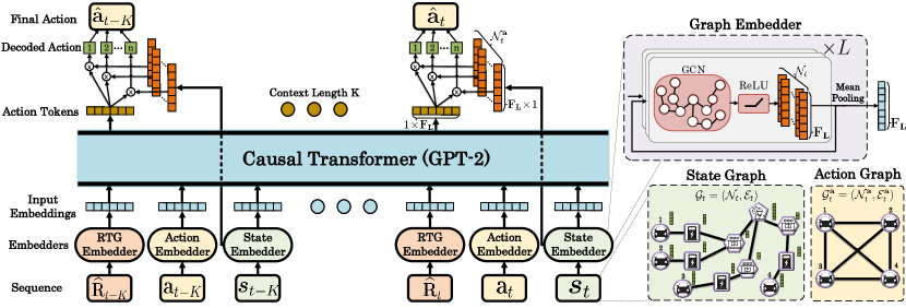
Figure 1: Overview of the GNN-DT architecture. The input sequence, comprising return-to-go, action, and state, is processed through specialized embedding modules. The action graph $\mathcal{G}^{\mathbf{a}}_{t}=(\mathcal{N}^{\mathbf{a}}_{t},\mathcal{E}^{\mathbf{a}}_{t})$, with nodes $\mathcal{N}^{\mathbf{a}}_{t}\subset\mathcal{N}_{t}$, and the state graph $\mathcal{G}_{t}=(\mathcal{N}_{t},\mathcal{E}_{t})$ are encoded using GNN-based embedders to produce embeddings of dimension $F_{L}$. These embeddings serve as inputs to a GPT-2–based causal transformer, which predicts the next action token. The predicted action token acts as a decoder, generating actions by multiplying with specific GNN state node embeddings. This architecture enables efficient decision-making in scenarios with dynamic states and actions.

The innovative GNN-DT architecture (Fig. 1) efficiently solves optimization problems in complex environments with dynamic state-action spaces by embedding past actions, states, and returns-to-go, using a causal transformer to generate action tokens, and integrating these with current state embeddings to determine final actions within the dynamically changing action space.

4.1 Sequence Embeddings

In GNN-DT, each input “modality” is processed by a specialized embedding network. The state graph passes through the State Embedder, the action through the Action Embedder, and the return-to-go value through a simple Multi-Layer Perceptron (MLP). Compared to standard MLP embedders, GNNs provide embeddings for states and actions invariant to the number of nodes by capturing the graph structure. This design makes GNN-DT more sample-efficient during training and better at generalizing to unseen environments.

In detail, the State Embedder consists of $L$ consecutive Graph Convolutional Network (GCN) (Kipf & Welling, 2016) layers, which aggregate information from neighboring nodes as follows:

$$\boldsymbol{x}_{t}^{(l+1)}=\sigma\Bigl{(}D^{-1/2}A_{t}D^{-1/2}\boldsymbol{x}_{t}^{(l)}W^{(l)}\Bigr{)},$$ (6)

where $\boldsymbol{x}_{t}^{(l)}\in\mathbb{R}^{N_{t}\times F_{l}}$ denotes the node embeddings at layer $l$ with $N_{t}$ number of nodes, $W^{(l)}\in\mathbb{R}^{F_{l}\times F_{l+1}}$ are trainable weights, $\sigma(\cdot)$ is a nonlinear activation (ReLU), $A_{t}$ is the adjacency matrix of the state graph $\mathcal{G}_{t}$, and $D$ is the degree matrix for normalization. After the final layer, a mean-pooling operation produces a fixed-size state embedding:

$$\boldsymbol{\widetilde{s}}_{t}=\frac{1}{\lvert\mathcal{N}_{t}\rvert}\sum_{n\in\mathcal{N}_{t}}\boldsymbol{x}_{n,t}^{(L)},$$ (7)

where $\boldsymbol{x}_{n}^{(L)}$ is the embedding of node $n$ at the $L$-th layer. This pooling step ensures that the state embedding is invariant to the number of nodes in the graph, enabling the architecture to scale with any number of EVs or chargers.

Similarly, the Action Embedder processes the action graph $\mathcal{G}^{\mathbf{a}}_{t}=(\mathcal{N}^{\mathbf{a}}_{t},\mathcal{E}^{\mathbf{a}}_{t})$ through $C$ GCN layers followed by mean pooling, producing the action embedding $\widetilde{\textbf{a}}_{t}$. All embedding vectors (states, actions, or the return-to-go value) have the same dimensions. This design leverages the dynamic and invariant nature of GCN-based embeddings, allowing the DT to handle variable-sized graphs.

4.2 Decoding Actions

Once the embedding sequence of length $K$ is constructed, it is passed through the causal transformer GPT-2 (Chen et al., 2021) to produce a fixed-size output vector $\boldsymbol{y}_{t}\in\mathbb{R}^{F_{L}}$ for each step. Because DT architectures inherently generate outputs of fixed dimensions, an additional mechanism is required to manage dynamic action spaces. To address this, GNN-DT implements a residual connection that merges the final GCN layer embeddings $\boldsymbol{x}_{t}^{(L)}$ with the transformer output $\boldsymbol{y}_{t}$ for every step of the sequence.

Specifically, for each node $n\in\mathcal{N}_{t}^{\mathbf{a}}$, we retrieve its corresponding state embedding $\boldsymbol{x}_{n,t}^{(L)}\in\mathbb{R}^{1\times F_{L}}$ and multiply it with the transformer output token $\boldsymbol{y}_{t}\in\mathbb{R}^{1\times F_{L}}$, yielding the final action for node $n$:

$$\hat{\mathrm{a}}_{n,t}=\boldsymbol{y}_{t}^{\mathsf{T}}\cdot\boldsymbol{x}_{n,t}^{(L)}.$$ (8)

By repeating Eq. 8 for every step $t$ and every node $n\in\mathcal{N}^{\mathbf{a}}_{t}$ the final action vector $\hat{\mathbf{a}}_{t}$ is generated. This design allows the model to maintain a fixed-size output from the DT while dynamically adapting to any number of nodes (and hence actions). It effectively combines the high-level context learned by the transformer with the node-specific state information captured by the GNN, enabling robust, scalable decision-making even as the graph structure changes.

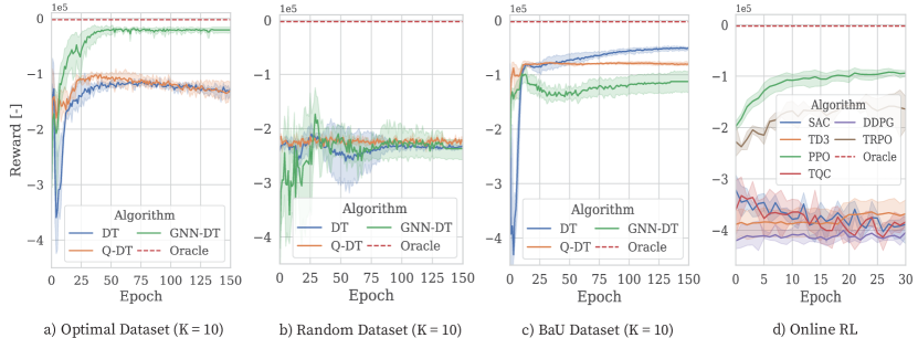
Figure 2: Training performance comparison of DT variations (classic DT, Q-DT, and GNN-DT) across 3 different datasets with 10.000 trajectories each and classic online RL algorithms for the same problem.

4.3 Action Masking and Loss Function

In GNN-DT, the learning of infeasible actions, such as charging an unavailable EV, is avoided through action masking. At each time step $t$, a mask vector $\mathbf{m}_{t}$, which has the same dimension as $\mathbf{a}_{t}$, is generated with zeros marking invalid actions and ones marking valid actions. For example, an action is invalid when the $a_{i,t}\neq 0$ and no EV is connected at charger $i$. The mean squared error between the predicted actions $\widehat{\mathbf{a}}_{t}$ and ground-truth actions $\mathbf{a}_{t}$ from expert or offline trajectories is employed as the loss function. For a window of length $K$ ending at time $t$, training loss is defined as:

$$\mathcal{L}=\frac{1}{K}\sum_{\tau=t-K}^{t}\|\left(\widehat{\mathbf{a}}_{\tau}-\mathbf{a}_{\tau}\right)\circ\mathbf{m}_{\tau}\|^{2}.$$ (9)

By incorporating the mask into the loss calculation (elementwise multiplication), a focus solely on valid actions is enforced, thereby preserving meaningful gradient updates and enhancing training stability.

5 Experiments

In this section, a comprehensive set of experiments is presented to evaluate the proposed method’s performance, both during training and under varied test conditions. Different dataset types and sample sizes are examined to determine their impact on learning efficiency and convergence, while generalization to unseen environments is also assessed.

Experimental Setup

The dataset generation and the evaluation experiments are conducted using the EV2Gym simulator (Orfanoudakis et al., 2024a), which leverages real-world data distributions, including EV arrivals, EV specifications, electricity prices, etc. This setup ensures a realistic environment where the state and action spaces accurately reflect real charging stations’ operational complexity. A scenario with 25 chargers is chosen, allowing up to 25 EVs to be connected simultaneously. In this configuration, the action vector has up to 25 variables (one per EV), while the state vector contains around 150 variables describing EV statuses, charger conditions, power transformer constraints, and broader environmental factors. Consequently, the resulting optimization problem is in the moderate-to-large scale range, reflecting the key complexities of real-world EV charging infrastructure. Each training procedure is repeated 10 times with distinct random seeds to ensure statistically robust findings. All reported rewards represent the average performance over 50 evaluation scenarios, each featuring different configurations (electricity prices, EV behavior, power limits, etc.).

Dataset Generation

Offline RL algorithms, including DTs, can learn optimal policies from trajectories without needing online interaction with the environment. Consequently, the quality of the gathered training trajectories has a substantial impact on the learning process. In this work, three distinct strategies were used to generate trajectories:

• Random Actions: Uniformly sampled actions in the range $[-1,1]$ were applied to the simulator.

• Business-as-Usual (BaU): A Round Robin charging policy commonly employed by CPOs, which sequentially allocates charging power among EVs to balance fairness and efficiency.

• Optimal Policies: Optimal solutions derived from solving offline the mathematical problem described in Section 3.2 for randomly generated scenarios.

Each trajectory consists of 300 state-action-reward-action mask tuples, with each timestep representing a 15-minute interval, resulting in a total of three simulated days. This combination of random, typical, and expert data provides a comprehensive basis for evaluating how GNN-DT learns from diverse offline trajectories.

Table 1: Comparison of maximum episode rewards ($\times 10^{5}$) achieved by baseline methods and GNN-DT across various datasets and context lengths ($K$). Rewards highlighted in bold indicate the highest value within each dataset and $K$ category.

Dataset	Avg. Training
Dataset Reward		K=2			K=10
			DT	Q-DT	GNN-DT (Ours)	DT	Q-DT	GNN-DT (Ours)
Random $100$	$-2.37$ ±$0.39$		$-1.91$	$-1.97$	$\mathbf{-0.82}$	$-2.12$	$-2.09$	$-1.16$
Random $1000$			$-1.93$	$-2.04$	$-0.86$	$-2.11$	$-2.01$	$-1.18$
Random $10000$			$-1.76$	$-2.04$	$-1.25$	$-1.81$	$-1.98$	$\mathbf{-0.98}$
BaU $100$	$-0.67$ ±$0.07$		$-0.79$	$-0.74$	$\mathbf{-0.59}$	$-0.79$	$-0.72$	$-0.56$
BaU $1000$			$-0.71$	$-0.66$	$-0.65$	$-0.64$	$-0.71$	$-0.57$
BaU $10000$			$-0.69$	$-0.66$	$-0.66$	$\mathbf{-0.44}$	$-0.74$	$-0.53$
Optimal $100$	$-0.01$ ±$0.01$		$-0.67$	$-0.91$	$-0.15$	$-1.12$	$-0.90$	$-0.14$
Optimal $1000$			$-0.63$	$-0.67$	$-0.10$	$-0.87$	$-0.86$	$-0.09$
Optimal $10000$			$-0.63$	$-0.80$	$\mathbf{-0.04}$	$-0.72$	$-0.90$	$\mathbf{-0.07}$

5.1 Training Performance

Fig. 2 compares the proposed GNN-DT against two baselines, classic DT and Q-DT, which both rely on flattened state representations due to their inability to directly process graph-structured data. In these baseline methods, empty chargers and unavailable actions are replaced by zeros, so the action vector is always the same size. Several well-known online RL algorithms from the Stable-Baselines 3 framework (Raffin et al., 2021) (SAC, DDPG, TD3, TRPO, PPO, and TQC) are also included to provide a performance benchmark for complex optimization tasks featuring both dense and sparse rewards. The offline RL algorithms (DT, Q-DT, and GNN-DT) are trained on three different datasets (Optimal, Random, and BaU), each comprising 10.000 trajectories. A red dotted line marks the oracle reward, which represents the experimental maximum achievable reward obtained by completing a full simulation without uncertainty. This oracle reward serves as an upper bound and helps contextualize the relative performance of each method.

In Figs. 2.a-c, the offline DT-based approaches use a context length $K=10$ and learn from pre-collected trajectories. As expected, the Optimal dataset provides the highest-quality information, enabling GNN-DT to converge rapidly toward near-oracle performance, while classic DT and Q-DT lag far behind, showcasing GNN-DTs improved sampling efficiency. With the Random dataset, the limited quality of data leads all methods to plateau at lower reward values, although GNN-DT still surpasses the other baselines. An intriguing behavior is observed in the BaU dataset, where classic DT initially experiences a substantial drop but later recovers to a final reward level exceeding that of Q-DT and GNN-DT. In contrast, the online RL algorithms displayed in Fig. 2.d struggle to achieve comparable improvements, suggesting that pure online exploration is insufficient for solving this complex EV charging optimization problem with sparse rewards. For completeness, Appendix B.2 contains the training curves for all algorithm-dataset-context length configurations used.

In Table 1, the maximum episode reward is compared for small, medium, and large datasets (100, 1.000, and 10.000 trajectories), under two different context lengths ($K=2$ and $K=10$). The left side of Table 1 reports the dataset type, the number of trajectories, and the average reward in each dataset. All baselines achieve performance above the Random dataset’s average reward. However, only GNN-DT consistently approaches the Optimal dataset’s performance, reaching as close as $-0.04\times 10^{5}$ compared to the $-0.01\times 10^{5}$ optimal reward. This advantage becomes especially evident at the largest dataset size (10.000 trajectories), highlighting the benefits of the graph-based embedding layer. Overall, GNN-DT outperforms the baselines across all datasets and both context lengths, with the single exception of the BaU dataset at $K=10$. Interestingly, a larger context window does not always translate into higher rewards, potentially due to the problem setting. Similarly, the dataset size appears to have minimal impact on Q-DT, whereas DT and GNN-DT generally improve with more trajectories. These findings underscore that both the quality and quantity of offline data, coupled with the GNN-DT architecture, are key to achieving superior performance.

Enhancing Training Datasets

Table 2: Maximum reward of GNN-DT trained on merged Optimal and Random datasets for $K\!=\!2$ and $K\!=\!10$. Notice that performance improves even though the average training dataset rewards are substantially lower, showing the importance of using diverse datasets in training DTs. Rewards highlighted in bold represent the highest values within each $K$ category.

Dataset	Total Traj.	Avg. Dataset Reward	GNN-DT Reward ($\times 10^{5}$)
			K=2	K=10
Random (Rnd.) 100%	$1000$	$-2.37$ ±$0.39$	$-0.863$	$-1.187$
Opt. 25% + Rnd. 75%	$1000$	$-1.78$ ±$1.07$	$-0.045$	$\mathbf{-0.020}$
Opt. 50% + Rnd. 50%	$1000$	$-1.18$ ±$1.19$	$\mathbf{-0.021}$	$-0.040$
Opt. 75% + Rnd. 25%	$1000$	$-0.60~$±$1.03$	$-0.073$	$-0.057$
Optimal (Opt.) 100%	$1000$	$-0.01$ ±$0.01$	$-0.108$	$-0.099$

The previous section highlighted that the quality of trajectories in the training dataset is the most influential factor for achieving high performance. In this section, we explore whether creating new datasets by mixing existing ones can further improve performance. Initially, the Optimal and Random datasets are combined in different proportions, as summarized in Table 2. A noteworthy result is that supplementing the Optimal dataset with theoretically less useful (Random) trajectories consistently boosts performance. In particular, GNN-DT with $K=10$, trained on a mix of 250 Optimal and 750 Random trajectories, achieves near-oracle results, deviating by only $-0.001\times 10^{5}$ from the optimal reward. A similar trend emerges when blending BaU and Random datasets (Table 3), although the performance gains are not as significant. Overall, these findings indicate that carefully integrating high- and lower-quality data can enhance policy learning beyond what purely Optimal or purely Random datasets can provide.

Table 3: Maximum reward of GNN-DT trained on merged BaU and Random datasets for $K=2$ and $K=10$.

Dataset	Total Traj.	Avg. Dataset Reward	GNN-DT Reward ($\times 10^{5}$)
			K=2	k=10
Random (Rnd.) 100%	$1000$	$-2.37$ ±$0.39$	$-0.863$	$-1.187$
BaU 25% + Rnd. 75%	$1000$	$-1.93$ ±$0.80$	$-0.578$	$-0.461$
BaU 50% + Rnd. 50%	$1000$	$-1.51$ ±$0.87$	$-0.665$	$\mathbf{-0.447}$
BaU 75% + Rnd. 25%	$1000$	$-1.09$ ±$0.76$	$\mathbf{-0.421}$	$-0.471$
BaU 100%	$1000$	$-0.01$ $\textpm 0.01$	$-0.654$	$-0.572$

Impact of larger context lengths (K)

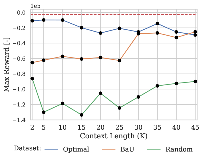
Figure 3: GNN-DT performance for larger context lengths (K).

Fig. 3 demonstrates that the context length $K$ plays a key role in the performance of GNN-DT, with diminishing returns beyond a certain point. For high-quality datasets like Optimal, moderate context lengths ($K=5$ to $K=10$) yield the best results, while larger $K$ values do not improve performance significantly. For suboptimal datasets like BaU and Random, the performance is lower overall, and longer context lengths seem to offer meaningful improvements, particularly when using the BaU dataset. Thus, selecting an appropriate context length is crucial for achieving better performance, while the quality of the dataset remains the most influential factor.

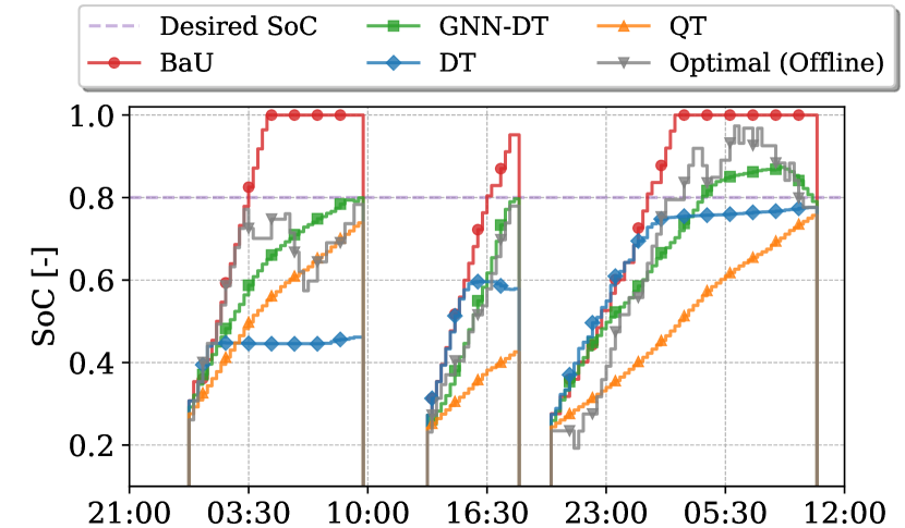
(a) EVs’ battery level progression over time.

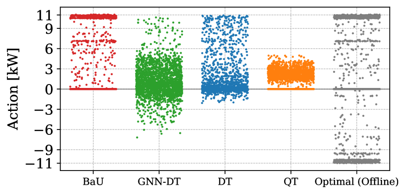
(b) Charger Actions

Figure 4: Comparison of smart charging algorithms based on (a) State of Charge, and (b) Action Probability.

5.2 Illustrative Example of EV Charging

With the models trained, we proceed to compare the behavior of the best baseline models trained (DT, Q-DT, GNN-DT) against the heuristic BaU algorithm in an EV charging scenario. Fig. 4a presents the SoC progress for three EVs connected one after the other to a single charger throughout the simulation, while Fig. 4b illustrates the charging and discharging actions of all chargers taken by each algorithm.

In Fig. 4a, the heuristic BaU algorithm consistently overcharges the EVs, often exceeding the desired SoC levels. In contrast, both DT and Q-DT fail to fully satisfy the desired SoC, except for the last EV, resulting in suboptimal performance. Conversely, GNN-DT successfully achieves the desired SoC for all EVs, closely mirroring the behavior of the optimal algorithm. This demonstrates GNN-DT’s ability to precisely control charging actions based on dynamic state information. Fig. 4b provides further insights into the actions taken by each algorithm. The optimal solution primarily employs maximum charging or discharging power, since it knows the future. In comparison, GNN-DT exhibits a more refined approach, modulating charging power within a range of -6 to 11 kW. On the other hand, baseline DT and Q-DT display a narrower range of actions, limiting their ability to optimize the charging schedules and adapt to varying conditions. These results underscore the superior capability of GNN-DT in managing the complexities of EV charging dynamics. For a more detailed analysis of key performance metrics in EV charging scenarios, refer to Appendix A.3.

5.3 Evaluation of Generalization and Scalability

Generalization Analysis

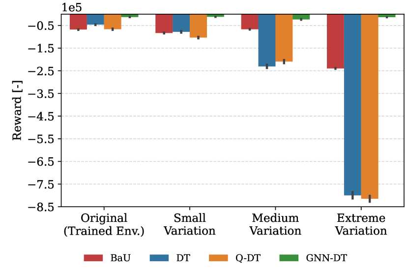
(a) Unseen state transition probabilities.

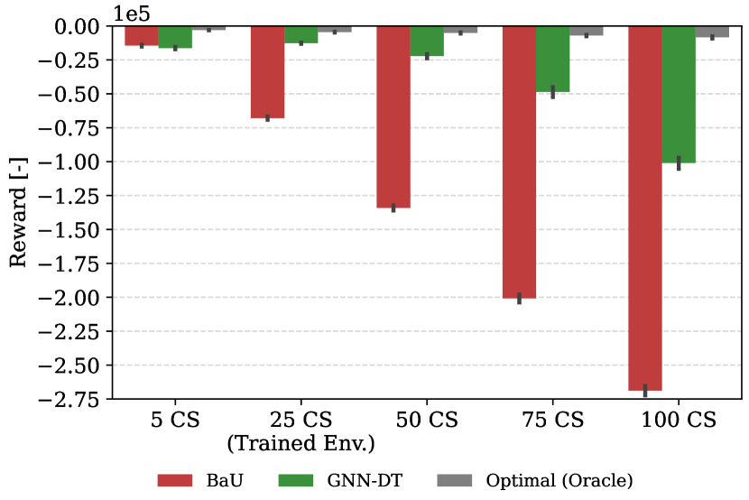
(b) Evaluating on different size problems.

Figure 5: Generalization performance of the proposed model, depicting the average rewards achieved across 100 randomly generated scenarios in previously unseen environments.

Evaluating the generalization of RL models across varying state transition probabilities is crucial for ensuring consistent performance under diverse conditions (Wang et al., 2020). In Fig. 5a, the generalization capabilities of GNN-DT and other baselines are assessed in environments with small, medium, and extreme variations in state transition probabilities (compared to the training environment). While the baseline methods experience significant performance drops as the evaluation environment deviates from the training setting, GNN-DT maintains strong performance across all scenarios. This highlights the critical role of GNN-based embeddings in improving model robustness and generalization.

A key advantage of the GNN-DT architecture, not present in classic DTs, is its invariance to problem size, i.e. the same network can be applied to both smaller and larger-scale environments. Fig. 5b illustrates the scalability and generalization performance of GNN-DT compared to the BaU algorithm and Optimal policy. GNN-DT, originally trained on a 25-charger environment, is evaluated in environments with 5, 50, 75, and 100 chargers. As expected, performance decreases as the number of chargers increases, since GNN-DT was not trained on larger-scale environments. Nevertheless, it still outperforms the heuristic BaU, demonstrating the model’s capability to handle problem size variation. In future work, training GNN-DT on a range of charger configurations simultaneously could further enhance its adaptability across a broader spectrum of environments.

Scalability Analysis

Table 4: Maximum reward achieved by GNN-DT in a large-scale EV charging optimization task involving 250 chargers.

	Total Trajectories	Avg. Dataset Reward	GNN-DT Reward
Random	$3000$	$-22.39$ ±$1.49$	$-9.34$
BaU	$3000$	$-6.67$ ±$0.32$	$-4.23$
Optimal	$3000$	$-0.08$ ±$0.03$	$\mathbf{-0.27}$

The scalability and effectiveness of GNN-DT were tested when trained on a significantly larger optimization problem involving 250 charging stations (CSs). In this scenario, the model must handle up to 250 action variables per step and over 1,000 state variables, which include critical information such as power limits and battery levels. The results presented in Table 4 demonstrate that GNN-DT shows promise for addressing more complex optimization tasks. However, the model requires a substantial increase in both the number of training trajectories and memory resources to maintain efficiency, highlighting a well-known limitation of DT-based approaches.

6 Conclusions

In this work, we introduced a novel DT-based architecture, GNN-DT, which incorporates GNN embedders to significantly enhance sample efficiency and overall performance. Through extensive evaluation across various datasets, including expert, random, and BaU, we demonstrated that traditional DTs and online RL algorithms fail to generalize effectively in real-world settings without specialized embeddings. We further show that both the size and quality of input trajectories critically impact the training process, underscoring the importance of carefully selecting datasets for effective learning. Finally, by leveraging the power of GNN embeddings, GNN-DT improved the model’s ability to generalize in previously unseen environments and handle large, complex action spaces. These contributions demonstrate GNN-DT’s potential to address complex dynamic optimization challenges beyond EV charging. They also underscore the critical roles of data quality and model architecture in enabling efficient real-world deployment.

Appendix A Appendix: EV Charging Model

The first appendix Section provides the complete mixed integer programming (MIP) formulation of the optimal EV charging problem and presents detailed experimental results for key evaluation metrics.

A.1 Complete EV charging MIP model

The optimal EV charging problem we investigate aims to maximize the CPO’s profits while ensuring that the demands of EV users are fully satisfied. The CPO lacks prior knowledge of when EVs will arrive or the aggregated power constraints. However, it is assumed that when an EV arrives at charging station $i$ initiating charging session $j$, it provides its departure time ($t_{j,i}^{d}$) and the desired battery capacity ($e^{*}_{j,i}$) at departure. Additionally, the battery capacity $e_{i,t}$ for each EV is known while it is connected to the charger. These assumptions are standard in research, as this information can typically be retrieved through evolving charging communication protocols.

The investigated EV charging problem expands over a simulation with $t$ timesteps, $t\in\mathcal{T}$ where a CPO decides the charging and discharging power ($p^{+}_{i,t}$ and $p^{-}_{i,t}$) for every charging station $i\in\mathcal{I}$. Since the chargers can be spread around the city, there are charger groups $w\in\mathcal{W}$, that can have a lower-level aggregated power limits representing connections to local power transformers. Based on these factors, the overall optimization objective is defined as follows:

$$\max_{p^{+},\omega^{+},p^{-},\omega^{-}}\sum_{t\in\mathcal{T}}\Bigg{(} -100\cdot\max\{0,p_{t}^{\sum}-p^{*}_{t}\}$$ (10)

$$+\sum_{i\in\mathcal{I}}\Bigg{(}\Delta t\left(\Pi^{+}_{t}p_{i,t}^{+}\omega^{+}_{i,t}-\Pi^{-}_{t}p_{i,t}^{-}\omega^{-}_{i,t}\right)$$ (11)

$$\quad-10\cdot\sum_{j\in\mathcal{J}_{i}}\left(\sum_{t=t_{j,i}^{a}}^{t_{j,i}^{d}}\left(p_{i,t}^{+}\omega^{+}_{i,t}-p_{i,t}^{-}\omega^{-}_{i,t}\right)-e^{*}_{j,i}\right)^{2}\Bigg{)}\Bigg{)}$$ (12)

Subject to:

$$p^{\sum}_{t}=\sum_{i\in\mathcal{I}}p^{+}_{i,t}\cdot\omega^{+}_{i,t}-p^{-}_{i,t}\cdot\omega^{-}_{i,t} \forall i,\;\forall t$$ (13)

$$\overline{p}_{w,t}\geq\sum_{i\in\mathcal{W}_{i}}p^{+}_{i,t}\cdot\omega^{+}_{i,t}-p^{-}_{i,t}\cdot\omega^{-}_{i,t} \forall i,\;\forall w,\;\forall t$$ (14)

$$\underline{e}_{j,i}\leq e_{j,i,t}\leq\overline{e}_{j,i} \forall j,\;\forall i,\;\forall t$$ (15)

$$e_{j,i,t}=e_{j,i,t-1}+(p^{+}_{i,t}\cdot\omega^{+}_{i,t}+p^{-}_{i,t}\cdot\omega^{-}_{i,t})\cdot\Delta t \forall j,\;\forall i,\;\forall t$$ (16)

$$e_{j,i,t}=e^{a}_{j,i,t} \forall j,\;\forall i,\;\forall t|\;t={t}^{a}_{j,i,t}$$ (17)

$$\underline{p}^{+}_{j,i}\leq p^{+}_{i,t}\leq\overline{p}^{+}_{j,i} \forall j,\;\forall i,\;\forall t$$ (18)

$$\underline{p}^{-}_{j,i}\geq p^{-}_{i,t}\geq\overline{p}^{-}_{j,i} \forall j,\;\forall i,\;\forall t$$ (19)

$$\omega^{+}_{i,t}+\omega^{-}_{i,t}\leq 1 \forall i,\;\forall t$$ (20)

The power of a single charger $i$ is modeled using four decision variables, $p^{+}\cdot\omega^{+}$ and $p^{-}\cdot\omega^{-}$, where $\omega^{+}$ and $\omega^{-}$ are binary variables, to differentiate between charging and discharging behaviors and enable charging power to get values in ranges $0\cup[\underline{p}^{+},\overline{p}^{+}]$, and discharging power in $[\underline{p}^{-},\overline{p}^{-}]\cup 0$. Eq. 14 defines the locally aggregated transformer power limits $\overline{p}$ for chargers belonging to groups $\mathcal{W}_{i}$. Eqs.(16) and(17) address EV battery constraints during operation with a minimum and maximum capacity of $\underline{e}$, $\overline{e}$, and energy $e^{a}$ at time of arrival $t^{a}$. Equations (18) and (19) impose charging and discharging power limits for every charger-EV session combination. To prevent simultaneous charging and discharging, the binary variables $\omega^{\text{ch}}$ and $\omega^{\text{dis}}$ are constrained by (20).

A.2 Evaluation Metrics

The following evaluation metrics are used in this study to assess the performance of the proposed algorithms:

User Satisfaction [%]: This metric measures how closely the state of charge (SoC) of an EV at departure matches its target $\text{SoC}^{*}$. For a set of EVs $\mathcal{J}$, user satisfaction is given by:

$$\textbf{User Sat.}=\frac{1}{|\mathcal{J}|}\cdot\sum_{j\in\mathcal{J}}\left(\frac{e_{j,t^{d}}}{e^{*}_{j}}\right)\cdot 100\%.$$ (21)

This ensures that each EV is charged to its desired level by the end of the charging session.

Energy Charged [kWh]: This represents the total energy supplied to EVs over the entire charging period and is given by:

$$\textbf{Energy Charged}=\sum_{t\in\mathcal{T}}\sum_{i\in\mathcal{I}}p^{+}_{i,t}\cdot\omega^{+}_{i,t}\cdot\Delta t.$$ (22)

This metric helps quantify the overall energy throughput for the system.

Energy Discharged [kWh]: This measures the amount of energy discharged back to the grid by the EVs. Discharging is typically done when electricity prices are high, and this metric is important for evaluating the system’s ability to contribute to grid stability.

$$\textbf{Energy Discharged}=\sum_{t\in\mathcal{T}}\sum_{i\in\mathcal{I}}p^{-}_{i,t}\cdot\omega^{-}_{i,t}\cdot\Delta t.$$ (23)

Power Violation [kW]: This metric tracks violations of operational constraints, such as exceeding the aggregated power limits at any given time. A violation occurs when the total power used exceeds the maximum allowed power:

$$\textbf{Power Violation}=\sum_{t\in\mathcal{T}}\max\{0,p_{t}^{\sum}-p^{*}_{t}\}\Delta t.$$ (24)

Minimizing this metric ensures that the system remains within operational limits and avoids overloading the grid.

Cost [€]: This evaluates the financial cost of the charging operations, considering both charging and discharging costs based on electricity prices. The total cost over the simulation period is defined as:

$$\textbf{Cost}=\sum_{t\in\mathcal{T}}\sum_{i\in\mathcal{I}}\Delta t(\Pi^{+}_{t}p_{i,t}^{+}-\Pi^{-}_{t}p_{i,t}^{-}),$$ (25)

This metric helps assess the cost-effectiveness of the charging strategy.

A.3 Complete Experimental Results of EV Charging.

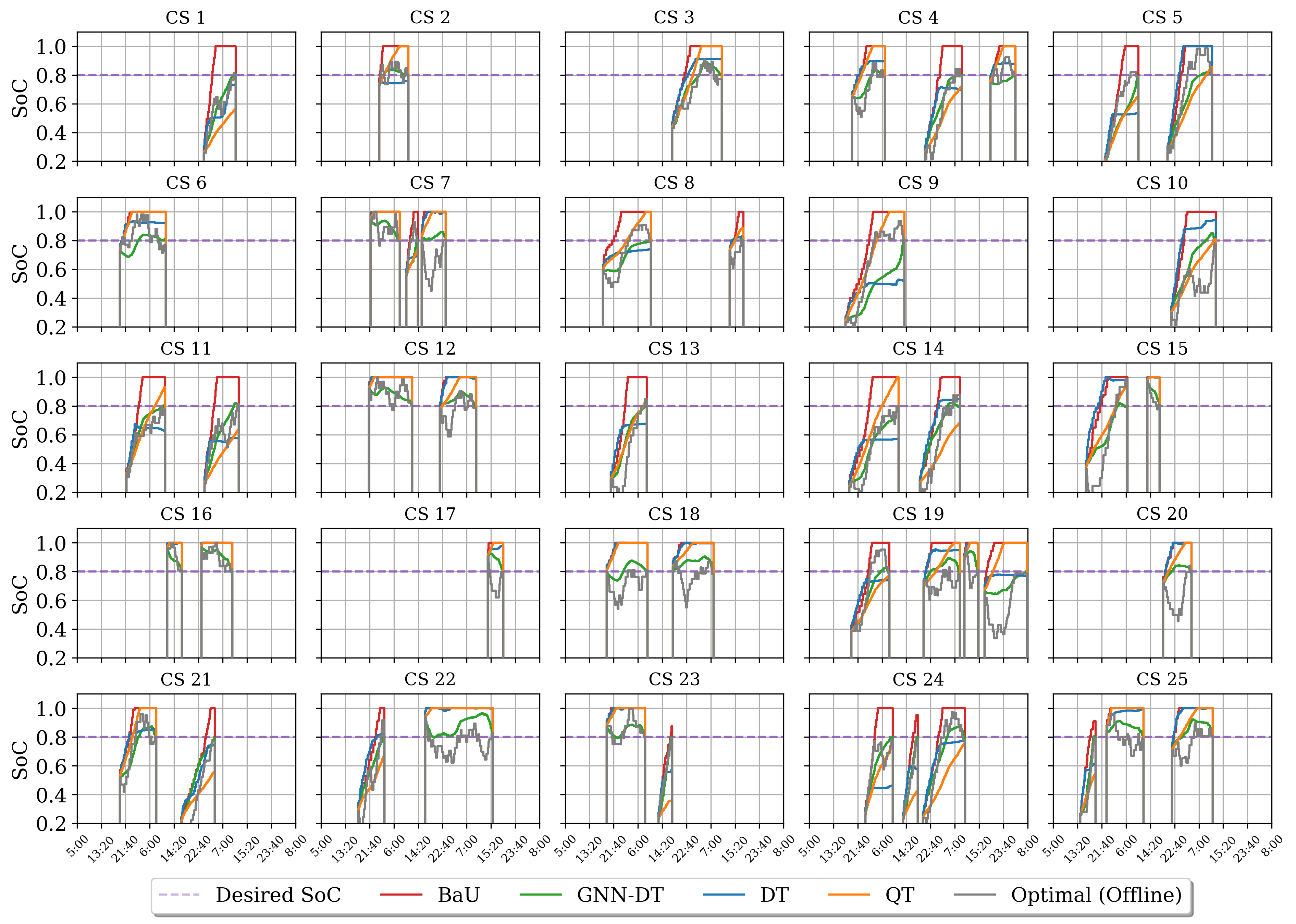
(a)

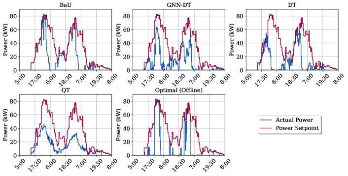
(b)

Figure 6: Complete results for a single evaluation scenario:(a) illustrating individual EV battery trajectories across all 25 charging stations, and (b) presenting the actual aggregate power usage against the power limit for the entire EV fleet.

Table 5 shows a comparison of key EV charging metrics for the 25-station problem after 100 evaluations, including heuristic algorithms, Charge As Fast as Possible (CAFAP) and BaU, and DT variants with the optimal solution, which assumes future knowledge. GNN-DT shows remarkable performance, achieving a close approximation to the optimal solution, particularly in user satisfaction (99.3% ± 0.03%) and power violation (21.7 ± 22.8 kW). It outperforms both BaU and DT variants in terms of energy discharged, power violation, and costs. Notably, GNN-DT performs well even compared to Q-DT, while maintaining competitive execution time, albeit slightly slower than the simpler models. The results underscore the effectiveness of GNN-DT in managing complex EV charging tasks, demonstrating its potential for real-world applications where future knowledge is not available.

Table 5: Comparison of key EV charging metrics for the 25-station problem after 100 evaluations, for heuristic algorithms (CAFAP & BaU) and DT variants with the optimal solution, which assumes future knowledge.

Algorithm	Energy
Charged
[MWh]	Energy
Discharged
[MWh]	User
Satisfaction
[%]	Power
Violation
[kW]	Costs
[€]	Reward
[-$10^{5}$]	Exec. Time
[sec/step]
CAFAP	$1.3$ ±$0.2$	$0.00$ ±$0.00$	$100.0$ ±$0.0$	$1289.2$ ±$261.8$	$-277$ ±$165$	$-1.974$ ±$0.283$	$0.001$
BaU	$1.3$ ±$0.2$	$0.00$ ±$0.00$	$99.9$ ±$0.2$	$10.5$ ±$9.4$	$-255$ ±$156$	$-0.679$ ±$0.067$	$0.001$
DT	$0.9$ ±$0.1$	$0.03$ ±$0.01$	$94.4$ ±$1.6$	$58.7$ ±$28.3$	$-173$ ±$104$	$-0.462$ ±$0.093$	$0.006$
Q-DT	$1.0$ ±$0.1$	$0.00$ ±$0.00$	$93.6$ ±$2.1$	$20.1$ ±$21.4$	$-187$ ±$113$	$-0.665$ ±$0.135$	$0.010$
GNN-DT (Ours)	$0.9$ ±$0.1$	$0.19$ ±$0.03$	$99.3$ ±$0.2$	$21.7$ ±$22.8$	$-142$ ±$89$	$-0.027$ ±$0.023$	$0.023$
Optimal (Offline)	$1.9$ ±$0.2$	$1.08$ ±$0.19$	$99.1$ ±$0.2$	$2.0$ ±$4.6$	$-119$ ±$84$	$-0.020$ ±$0.015$	-

Fig. 6 presents the results from a single evaluation scenario, focusing on the performance of various charging strategies across all 25 charging stations. Fig. 6a illustrates the individual battery trajectories for each EV across the stations, showing how the actual SoC evolves over time. The desired SoC is compared against the results from different algorithms: BaU, GNN-DT, DT, Q-DT, and the Optimal (Offline) solution. It is evident that GNN-DT closely tracks the desired SoC across all stations, outperforming the other methods, particularly in terms of maintaining the target SoC. Fig. 6b provides insights into the aggregate power usage of the entire EV fleet, where the actual power used is compared to the setpoint power. GNN-DT closely aligns with the power setpoint, demonstrating effective power management, while other methods such as BaU and Q-DT show greater deviations, indicating less efficient power usage. These results underline the superior performance of GNN-DT in optimizing charging strategies while adhering to power constraints.

Appendix B Appendix: Training

Here, we present the hyperparameter settings used for training DT, Q-DT, and GNN-DT, accompanied by detailed training curves that illustrate the convergence of each model.

B.1 Training Hyperparameters

Table 6: Algorithm hyperparameters.

Hyperparameter	Value
Batch Size	$64$ (for large scale), $128$ (for small scale)
Learning Rate	$10^{-4}$
Weight Decay	$10^{-4}$
Number of Steps per Iteration	$1000$
Number of Decoder Layers	$3$
Number of Attention Heads	$4$
Embedding Dimension	$256$
GNN Embedder Feature Dimension	$16$
GNN Hidden Dimension	$32$ (for small scale), $64$ (for large scale)
Number of GCN Layers	$3$
Maximum Epochs	$250$ (for small scale), $400$ (for large scale)
Number of Steps per Iteration	$1000$ (for small scale), $3000$ (for large scale)
Embedding Dimension	$128$ (for small scale), $256$ (for large scale)
Memory per CPU (GB)	$8$ (for small scale), $16$ or $40$ (for large scale)
Time Limit (hours)	$10$ (for small scale), $20$ or $46$ (for large scale)

B.2 Detailed Training Curves

Fig. 7 provides a detailed comparison of training curves for various algorithm-dataset-context length ($K$) combinations, highlighting the significant impact of the training sample size on performance. The figure includes training results for DT, Q-DT, and GNN-DT across different datasets (Optimal, Random, and BaU) and context lengths ($K=2$ and $K=10$), with each plot showing the performance for 100, 1,000, and 10,000 trajectory samples.

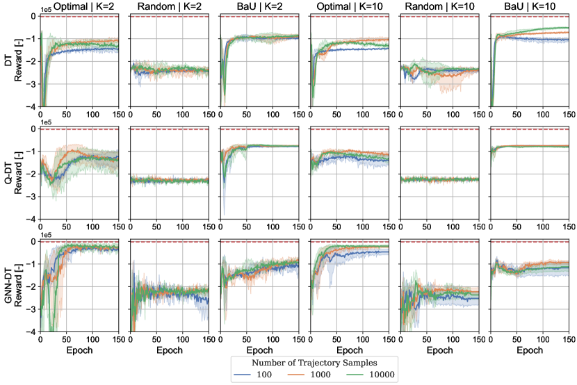
Figure 7: Complete comparison of training curves for combinations of algorithms-K-training dataset for different numbers of samples.

B.3 Mixed Dataset Training Curves

Fig. 8 presents the learning curves for the mixed datasets approach, comparing performance across various combinations of Optimal, Random, and BaU datasets for both $K=2$ and $K=10$. Fig. 8a illustrates the results for mixed Optimal datasets, where different proportions of the Optimal and Random datasets (e.g., 50% Optimal + 50% Random) are used for training. The performance becomes more unstable as more Random data is included. Interestingly, the performance for all the mixed datasets demonstrates better maximum reward reached compared to the Optimal-only dataset, highlighting the benefits of combining high-quality and lower-quality data. Fig. 8b shows similar trends for the Mixed-BaU datasets. While the BaU dataset alone performs worse than the Optimal dataset, mixing it with Random data still yields improvements, with the 75% BaU and 25% Random combination showing the best results. The results underscore the potential of mixing datasets to improve training performance, especially when high-quality data (Optimal or BaU) is supplemented with lower-quality Random data.

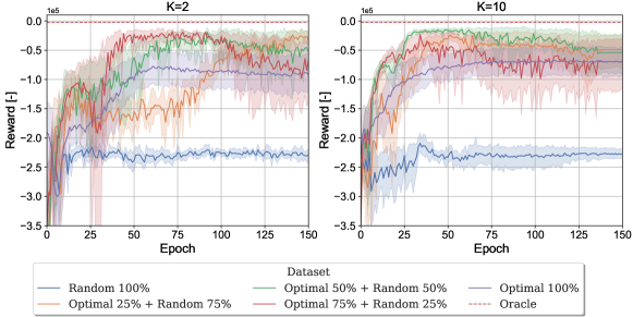
(a) Mixed-Optimal

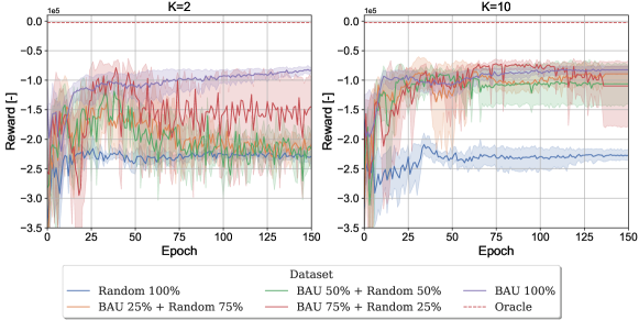
(b) Mixed-BaU

Figure 8: Mixed datasets learning curves for optimal and BaU.

References

- Bubeck (2015) Bubeck, S. Convex Optimization: Algorithms and Complexity. Now Foundations and Trends, 2015. doi: 10.1561/2200000050.
- Chen & Shi (2022) Chen, G. and Shi, X. A deep reinforcement learning-based charging scheduling approach with augmented lagrangian for electric vehicle, 2022.
- Chen et al. (2021) Chen, L., Lu, K., Rajeswaran, A., Lee, K., Grover, A., Laskin, M., Abbeel, P., Srinivas, A., and Mordatch, I. Decision transformer: Reinforcement learning via sequence modeling, 2021.
- Dulac-Arnold et al. (2021) Dulac-Arnold, G., Levine, N., Mankowitz, D. J., Li, J., Paduraru, C., Gowal, S., and Hester, T. Challenges of real-world reinforcement learning: definitions, benchmarks and analysis. Machine Learning, 110(9):2419–2468, September 2021. ISSN 1573-0565. doi: 10.1007/s10994-021-05961-4. URL https://doi.org/10.1007/s10994-021-05961-4.
- Gunjan & Bhattacharyya (2023) Gunjan, A. and Bhattacharyya, S. A brief review of portfolio optimization techniques. Artificial Intelligence Review, 56(5):3847–3886, 2023.
- Gupta & Gupta (2020) Gupta, K. and Gupta, M. K. (eds.). Optimization of Manufacturing Processes. Springer Series in Advanced Manufacturing, 2020.
- Hong et al. (2024) Hong, K., Li, Y., and Tewari, A. A primal-dual-critic algorithm for offline constrained reinforcement learning. In Dasgupta, S., Mandt, S., and Li, Y. (eds.), Proceedings of The 27th International Conference on Artificial Intelligence and Statistics, volume 238 of Proceedings of Machine Learning Research, pp. 280–288. PMLR, 02–04 May 2024. URL https://proceedings.mlr.press/v238/hong24a.html.
- Hu et al. (2024) Hu, S., Fan, Z., Huang, C., Shen, L., Zhang, Y., Wang, Y., and Tao, D. Q-value regularized transformer for offline reinforcement learning. In Forty-first International Conference on Machine Learning, 2024. URL https://openreview.net/forum?id=ojtddicekd.
- Jaimungal (2022) Jaimungal, S. Reinforcement learning and stochastic optimisation. Finance and Stochastics, 26(1):103–129, January 2022. ISSN 1432-1122. doi: 10.1007/s00780-021-00467-2. URL https://doi.org/10.1007/s00780-021-00467-2.
- Jin & Xu (2021) Jin, J. and Xu, Y. Optimal policy characterization enhanced actor-critic approach for electric vehicle charging scheduling in a power distribution network. IEEE Transactions on Smart Grid, 12(2):1416–1428, 2021. doi: 10.1109/TSG.2020.3028470.
- Jin et al. (2022) Jin, R., Zhou, Y., Lu, C., and Song, J. Deep reinforcement learning-based strategy for charging station participating in demand response. Applied Energy, 328:120140, 2022. ISSN 0306-2619. doi: https://doi.org/10.1016/j.apenergy.2022.120140. URL https://www.sciencedirect.com/science/article/pii/S0306261922013976.
- Kamrani et al. (2025) Kamrani, A. S., Dini, A., Dagdougui, H., and Sheshyekani, K. Multi-agent deep reinforcement learning with online and fair optimal dispatch of ev aggregators. Machine Learning with Applications, pp. 100620, 2025. ISSN 2666-8270. doi: https://doi.org/10.1016/j.mlwa.2025.100620. URL https://www.sciencedirect.com/science/article/pii/S2666827025000039.
- Kipf & Welling (2016) Kipf, T. N. and Welling, M. Semi-supervised classification with graph convolutional networks, 2016.
- Konstantakopoulos et al. (2022) Konstantakopoulos, G. D., Gayialis, S. P., and Kechagias, E. P. Vehicle routing problem and related algorithms for logistics distribution: a literature review and classification. Operational Research, 22(3):2033–2062, July 2022. ISSN 1866-1505. doi: 10.1007/s12351-020-00600-7. URL https://doi.org/10.1007/s12351-020-00600-7.
- Lai et al. (2023) Lai, Y., Liu, J., Tang, Z., Wang, B., Hao, J., and Luo, P. ChiPFormer: Transferable chip placement via offline decision transformer. In Krause, A., Brunskill, E., Cho, K., Engelhardt, B., Sabato, S., and Scarlett, J. (eds.), Proceedings of the 40th International Conference on Machine Learning, volume 202 of Proceedings of Machine Learning Research, pp. 18346–18364. PMLR, 23–29 Jul 2023. URL https://proceedings.mlr.press/v202/lai23c.html.
- Lan et al. (2023) Lan, Q., Mahmood, A. R., Yan, S., and Xu, Z. Learning to optimize for reinforcement learning, 2023.
- Lee et al. (2024) Lee, K.-H., Nachum, O., Yang, M., Lee, L., Freeman, D., Xu, W., Guadarrama, S., Fischer, I., Jang, E., Michalewski, H., and Mordatch, I. Multi-game decision transformers. In Proceedings of the 36th International Conference on Neural Information Processing Systems, NIPS ’22, Red Hook, NY, USA, 2024. Curran Associates Inc. ISBN 9781713871088.
- Levine et al. (2020) Levine, S., Kumar, A., Tucker, G., and Fu, J. Offline reinforcement learning: Tutorial, review, and perspectives on open problems, 2020.
- Li et al. (2022) Li, S., Hu, W., Cao, D., Dragičević, T., Huang, Q., Chen, Z., and Blaabjerg, F. Electric vehicle charging management based on deep reinforcement learning. Journal of Modern Power Systems and Clean Energy, 10(3):719–730, 2022. doi: 10.35833/MPCE.2020.000460.
- Liu et al. (2023) Liu, Z., Guo, Z., Yao, Y., Cen, Z., Yu, W., Zhang, T., and Zhao, D. Constrained decision transformer for offline safe reinforcement learning, 2023.
- Orfanoudakis et al. (2024a) Orfanoudakis, S., Diaz-Londono, C., Yılmaz, Y. E., Palensky, P., and Vergara, P. P. Ev2gym: A flexible v2g simulator for ev smart charging research and benchmarking. IEEE Transactions on Intelligent Transportation Systems, pp. 1–12, 2024a. doi: 10.1109/TITS.2024.3510945.
- Orfanoudakis et al. (2024b) Orfanoudakis, S., Robu, V., Salazar Duque, E. M., et al. Scalable reinforcement learning for large-scale coordination of electric vehicles using graph neural networks. Preprint (Version 1) available at Research Square, December 2024b. URL https://doi.org/10.21203/rs.3.rs-5504138/v1. Accessed on 19 December 2024.
- Panda & Tindemans (2024) Panda, N. K. and Tindemans, S. H. Quantifying the aggregate flexibility of ev charging stations for dependable congestion management products: A dutch case study, 2024.
- Paster et al. (2024) Paster, K., McIlraith, S. A., and Ba, J. You can’t count on luck: why decision transformers and rvs fail in stochastic environments. In Proceedings of the 36th International Conference on Neural Information Processing Systems, NIPS ’22, Red Hook, NY, USA, 2024. Curran Associates Inc. ISBN 9781713871088.
- Qiu et al. (2023) Qiu, D., Wang, Y., Hua, W., and Strbac, G. Reinforcement learning for electric vehicle applications in power systems:a critical review. Renewable and Sustainable Energy Reviews, 173:113052, 2023. ISSN 1364-0321. doi: https://doi.org/10.1016/j.rser.2022.113052. URL https://www.sciencedirect.com/science/article/pii/S1364032122009339.
- Raffin et al. (2021) Raffin, A., Hill, A., Gleave, A., Kanervisto, A., Ernestus, M., and Dormann, N. Stable-baselines3: Reliable reinforcement learning implementations. Journal of Machine Learning Research, 22(268):1–8, 2021. URL http://jmlr.org/papers/v22/20-1364.html.
- Roald et al. (2023) Roald, L. A., Pozo, D., Papavasiliou, A., Molzahn, D. K., Kazempour, J., and Conejo, A. Power systems optimization under uncertainty: A review of methods and applications. Electric Power Systems Research, 214:108725, 2023. ISSN 0378-7796. doi: https://doi.org/10.1016/j.epsr.2022.108725. URL https://www.sciencedirect.com/science/article/pii/S0378779622007842.
- Sadeghianpourhamami et al. (2020) Sadeghianpourhamami, N., Deleu, J., and Develder, C. Definition and evaluation of model-free coordination of electrical vehicle charging with reinforcement learning. IEEE Transactions on Smart Grid, 11(1):203–214, 2020. doi: 10.1109/TSG.2019.2920320.
- Sutton & Barto (2018) Sutton, R. S. and Barto, A. G. Reinforcement learning: An introduction. MIT press, 2018.
- Villarrubia-Martin et al. (2023) Villarrubia-Martin, E., Rodriguez-Benitez, L., Jimenez-Linares, L., Muñoz-Valero, D., and Liu, J. A hybrid online off-policy reinforcement learning agent framework supported by transformers. International Journal of Neural Systems, 33(12), October 2023. ISSN 0129-0657. doi: 10.1142/s012906572350065x.
- Wang (2024) Wang, B. Domain Adaptation in Reinforcement Learning: Approaches, Limitations, and Future Directions. Journal of The Institution of Engineers (India): Series B, 105(5):1223–1240, October 2024. ISSN 2250-2114. doi: 10.1007/s40031-024-01049-4. URL https://doi.org/10.1007/s40031-024-01049-4.
- Wang et al. (2020) Wang, R., Foster, D. P., and Kakade, S. M. What are the statistical limits of offline rl with linear function approximation?, 2020.
- Wu et al. (2024) Wu, Y.-H., Wang, X., and Hamaya, M. Elastic decision transformer. In Proceedings of the 37th International Conference on Neural Information Processing Systems, NIPS ’23, Red Hook, NY, USA, 2024. Curran Associates Inc.
- Yılmaz et al. (2024) Yılmaz, Y. E., Orfanoudakis, S., and Vergara, P. P. Reinforcement learning for optimized ev charging through power setpoint tracking. In 2024 IEEE PES Innovative Smart Grid Technologies Europe (ISGT EUROPE), pp. 1–5, 2024.
- Zhang et al. (2023a) Zhang, J., Liu, C., Li, X., Zhen, H.-L., Yuan, M., Li, Y., and Yan, J. A survey for solving mixed integer programming via machine learning. Neurocomputing, 519:205–217, 2023a. ISSN 0925-2312. doi: https://doi.org/10.1016/j.neucom.2022.11.024. URL https://www.sciencedirect.com/science/article/pii/S0925231222014035.
- Zhang et al. (2023b) Zhang, S., Jia, R., Pan, H., and Cao, Y. A safe reinforcement learning-based charging strategy for electric vehicles in residential microgrid. Applied Energy, 348:121490, 2023b. ISSN 0306-2619. doi: https://doi.org/10.1016/j.apenergy.2023.121490. URL https://www.sciencedirect.com/science/article/pii/S0306261923008541.
- Zhang et al. (2023c) Zhang, Z., Mei, H., and Xu, Y. Continuous-time decision transformer for healthcare applications. Proceedings of Machine Learning Research, 206:6245–6262, April 2023c.
- Zheng et al. (2022) Zheng, Q., Zhang, A., and Grover, A. Online decision transformer. In Chaudhuri, K., Jegelka, S., Song, L., Szepesvari, C., Niu, G., and Sabato, S. (eds.), Proceedings of the 39th International Conference on Machine Learning, volume 162 of Proceedings of Machine Learning Research, pp. 27042–27059. PMLR, 17–23 Jul 2022. URL https://proceedings.mlr.press/v162/zheng22c.html.