Summing large Pomeron loops in the saturation region: dipole-nucleus collision beyond nonlinear equations.

Abstract

In this paper we found the dipole-nucleus scattering amplitude at high energies by summing large Pomeron loops. It turns out that the energy dependence of this amplitude is the same as for dipole-dipole scattering. It means that the Balitsky-Kovchegov (BK) equation, which has been derived to describe this scattering, can be trusted only in the limited range of considerably low energies: $z\,\leq\,\sqrt{2\,\kappa\,C}A^{1/6}$

I Introduction

The goal of this paper is to sum the large BFKL Pomeron loopsBFKL for dipole-nucleus scattering at high energies. The scattering amplitude of this process satisfies the nonlinear equation which has been derived in momentumGLR ; MUQI and coordinate MUDI ; B ; K representation using different techniqueBART ; BRAUN ; BRN ; MV ; JIMWLK1 ; JIMWLK2 ; JIMWLK3 ; JIMWLK4 ; JIMWLK5 ; JIMWLK6 ; JIMWLK7 ; JIMWLK8 ; LELU . However, recently it has been shownKLLL1 ; KLLL2 that this nonlinear BK equation , that governs the dilute-dense parton density scattering (deep inelastic scattering (DIS) of electron with nuclei), has to be modified due to contributions of Pomeron loops. Indeed, in the BFKL Pomeron calculus the BK equation stems from summing the ‘fan’ Pomeron diagrams of Fig. 1-a GLR ; BRAUN . The enhanced Pomeron diagrams with the Pomeron loops (see Fig. 1-b) certainly lead to an additional contribution which we are going to estimate in this paper at ultra high energies. It is well known that in spite of intensive work BFKL ; KOLEB ; MUSA ; LETU ; LELU1 ; LIP ; KO1 ; LE11 ; RS ; KLremark2 ; SHXI ; KOLEV ; nestor ; LEPRI ; LMM ; LEM ; MUT ; MUPE ; IIML ; LIREV ; LIFT ; GLR ; GLR1 ; MUQI ; MUDI ; Salam ; NAPE ; BART ; BKP ; MV ; KOLE ; BRN ; BRAUN ; B ; K ; KOLU ; JIMWLK1 ; JIMWLK2 ; JIMWLK3 ; JIMWLK4 ; JIMWLK5 ; JIMWLK6 ; JIMWLK7 ; JIMWLK8 ; AKLL ; KOLU11 ; KOLUD ; BA05 ; SMITH ; KLW ; KLLL1 ; KLLL2 ; kl ; LEPR ; LE1 ; LE2 , the problem of summation of the Pomeron loops has not been solved.

In our recent paperLEDIDI we have suggested the way to sum the large Pomeron loops for dipole-dipole scattering deeply in the saturation region. In this paper the large Pomeron loops is summed using the $t$-channel unitarity, which has been rewritten in the convenient form for the dipole approach to CGC in Refs.MUSA ; Salam ; IAMU ; IAMU1 ; KOLEB ; MUDI ; LELU ; KO1 ; LE11 (see Fig. 2). The analytic expression takes the form LELU ; KO1 ; LE1 :

$$A\left(Y,r,R;\bm{b}\right)\,=$$ (1)

$$\,\sum^{\infty}_{n=1}\,\left(-1\right)^{n+1}\,n!\int\prod^{n}_{i}d^{2}r_{i}\,d^{2}\,r^{\prime}_{i}\,d^{2}b^{\prime}_{i}\int\!\!d^{2}\delta b_{i}\,\gamma^{BA}\left(r_{1},r^{\prime}_{i},\bm{b}_{i}-\bm{b^{\prime}_{i}}\equiv\delta\bm{b}_{i}\right)\,\,\rho^{P}_{n}\left(Y-Y_{0},\{\bm{r}_{i},\bm{b}_{i}\}\right)\,\rho^{T}_{n}\left(Y_{0},\{\bm{r}^{\prime}_{i},\bm{b}^{\prime}_{i}\}\right)$$

$\gamma^{BA}$ is the scattering amplitude of two dipoles in the Born approximation of perturbative QCD. The parton densities: $\rho^{P}_{i}Y,\{\bm{r}_{i},\bm{b}_{i}\}$ for projectile and $\rho^{T}_{i}Y,\{\bm{r}_{i},\bm{b}_{i}\}$ for target, have been introduced in Ref.LELU as follows:

$$\rho_{n}(r_{1},b_{1}\,\ldots\,,r_{n},b_{n};Y\,-\,Y_{0})\,=\,\frac{1}{n!}\,\prod^{n}_{i=1}\,\frac{\delta}{\delta u_{i}}\,Z\left(Y\,-\,Y_{0};\,[u]\right)|_{u=1}$$ (2)

where the generating functional $Z$ is

$$Z\left(Y,\bm{r},\bm{b};[u_{i}]\right)\,\,=\,\,\sum^{\infty}_{n=1}\int P_{n}\left(Y,\bm{r},\bm{b};\{\bm{r}_{i}\,\bm{b}_{i}\}\right)\prod^{n}_{i=1}u\left(\bm{r}_{i}\,\bm{b}_{i}\right)\,d^{2}r_{i}\,d^{2}b_{i}$$ (3)

where $u\left(\bm{r}_{i}\,\bm{b}_{i}\right)\equiv\,u_{i}$ is an arbitrary function and $P_{n}$ is the probability to have $n$ dipoles with the given kinematics. The initial and boundary conditions for the BFKL cascade stem from one dipole has the following form for the functional $Z$:

$$Z\left(Y=0,\bm{r},\bm{b};[u_{i}]\right) \,\,=\,\, u\left(\bm{r},\bm{b}\right);$$ (4a)

$$Z\left(Y,r,[u_{i}=1]\right) = 1;$$ (4b)

In Eq. (1) $\bm{b}_{i}\,\,=\,\,\bm{b}\,-\,\bm{b^{\prime}}_{i}$.

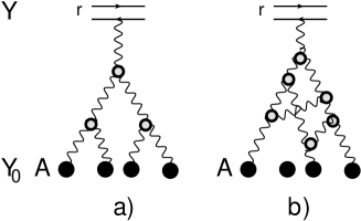
Figure 1: Fig. 1-a: The example of ‘fan’ BFKL Pomeron diagrams that lead to non-linear BK equation. Fig. 1-b: The example of the Pomeron loop diagrams ( enhanced diagrams) that we are summing in this paper at very high energy.Fig. 1-c: $t$-channel unitarity for the BFKL Pomeron. The double helix lines denote the reggeizied gluons. The wavy lines denote the BFKL Pomeron exchanges. The black circles denote the amplitude $\gamma^{BA}$ for interaction of the dipole with the nucleon which we replaced by the dipoles of the size $r^{\prime}$(see Fig. 2). The gray circles stand for the triple Pomeron vertex.

The parton densities for the projectile (fast dipole) have been found in Ref.LEDIDI . For completeness of presentation we will discuss them in the next section. However we wish to stress here that they satisfy both the evolution equations and the recurrence relations derived in QCD (see Refs.LELU ; LELU1 ; LE1 ; and the analytic solution to the nonlinear BK equation of Ref.LETU . This solution takes the form:

$$N^{\rm DIS}\left(z=r^{2}Q^{2}_{s}\left(Y,b\right)\right)\,\,=\,\,1\,\,-\,\,C(z)\exp\left(-\frac{z^{2}}{2\,\kappa}\right)$$ (5)

where $z=\ln\left(r^{2}Q^{2}_{s}(Y)\right)$ One can see that this solution shows the geometric scaling behaviour GS being a function of one variable. Function $C\left(z\right)$ is a smooth function which can be considered as a constant in our approach.

As one can see from Eq. (5) it turns out that BK equation leads to a new dimensional scale: saturation momentumGLR which has the following $Y$ dependenceGLR ; MUT ; MUPE :

$$Q^{2}_{s}\left(Y,b\right)\,\,=\,\,Q^{2}_{s}\left(Y=0,b\right)\,e^{\bar{\alpha}_{S}\,\kappa\,Y,-\,\,\frac{3}{2\,\gamma_{cr}}\ln Y}$$ (6)

where $Y=0$ is the initial value of rapidity and $\kappa$ and $\gamma_{cr}$ are determined by the following equations:

$$\kappa\,\,\equiv\,\,\frac{\chi\left(\gamma_{cr}\right)}{1-\gamma_{cr}}\,\,=\,\,-\frac{d\chi\left(\gamma_{cr}\right)}{d\gamma_{cr}}~$$ (7)

where $\chi\left(\gamma\right)$ is given by

$$\omega\left(\bar{\alpha}_{S},\gamma\right)\,\,=\,\,\bar{\alpha}_{S}\,\chi\left(\gamma\right)\,\,\,=\,\,\,\bar{\alpha}_{S}\left(2\psi\left(1\right)\,-\,\psi\left(\gamma\right)\,-\,\psi\left(1-\gamma\right)\right)$$ (8)

$\psi(z)$ is the Euler $\psi$ function (see Ref.RY formulae 8.36).

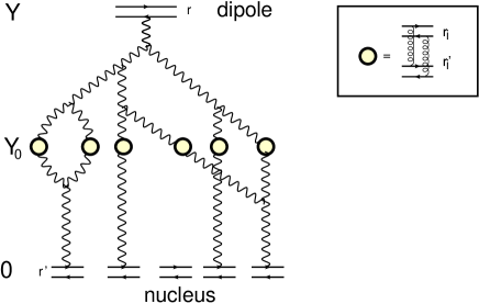
Figure 2: Summing large Pomeron loops for dipole-nucleus scattering. The wavy lines denote the BFKL Pomeron exchanges. The circles denote the amplitude $\gamma$ in the Born approximation of perturbative QCD. A nucleus is viewed as the bag of dipoles with the size $r^{\prime}$.

In the next section we show how to reconcile this solution with the fact that the BK equation is summing the ’fan’ diagrams of Fig. 1-a in the BFKL Pomeron calculus. We present Eq. (5) as a sum of many Pomerons exchanges and in doing so we find the parton densities $\rho_{n}$.

In section III we estimate the scattering amplitude using Eq. (1) and the parton densities that we found in section II. In conclusion we summarize our results and discuss possible flaw in our approach,

II Dipole densities $\rho_{n}\left(r,b,\{r_{i},b_{i}\}\right)$

II.1 The BFKL Pomeron Green’s function( $\rho_{1}\left(r,b,r_{1}b_{1}\right)$) in the saturation region

The Green’s function for the BFKL Pomeron exchange satisfy the linear equationBFKL which has the form:

$$\frac{\partial\,G_{I\!\!P}\left(Y,\bm{r};\bm{b}\right)}{\partial\,Y}=\bar{\alpha}_{S}\int\limits\frac{d^{2}r^{\prime}}{2\,\pi}\frac{r^{2}}{r^{\prime 2}\left(\bm{r}-\bm{r}^{\prime}\right)^{2}}\,\Bigg{\{}G_{I\!\!P}\left(Y,\bm{r}^{\prime};\bm{b}-\frac{1}{2}\left(\bm{r}-\bm{r}^{\prime}\right)\right)+G_{I\!\!P}\left(Y,\bm{r}-\bm{r}^{\prime};\bm{b}-\frac{1}{2}\bm{r}^{\prime}\right)-G_{I\!\!P}\left(Y,\bm{r};\bm{b}\right)\Bigg{\}}$$ (9)

Solution to this equation is the sum over the eigenfunction $\phi_{\gamma}\left(\bm{r},\bm{r}_{1},\bm{b}\right)$ with the eigenvalues $\bar{\alpha}_{S}\chi\left(\gamma\right)$:

$$G_{I\!\!P}\left(Y,\bm{r},\bm{r}_{1};\bm{b}\right)\,\,=\,\,\!\!\!\int\limits^{\epsilon+i\infty}_{\epsilon-i\infty}\!\!\!\frac{d\gamma}{2\,\pi\,i}e^{\bar{\alpha}_{S}\chi\left(\gamma\right)\,Y}\,\phi_{\gamma}\left(\bm{r},\bm{r}_{1},\bm{b}\right)\phi_{in}\left(r_{1}\right)$$ (10)

The eigenfunction $\phi_{\gamma}\left(\bm{r},\bm{r}_{1},\bm{b}\right)$ (the scattering amplitude of two dipoles with sizes $r$ and $r_{1}$) is equal to LIP

$$\phi_{\gamma}\left(\bm{r},\bm{r}_{1},\bm{b}\right)\,\,\,=\,\,\,\left(\frac{r^{2}\,r_{1}^{2}}{\left(\bm{b}+\frac{1}{2}(\bm{r}-\bm{r}_{1})\right)^{2}\,\left(\bm{b}-\frac{1}{2}(\bm{r}-\bm{r}_{1})\right)^{2}}\right)^{\gamma}=e^{\gamma\,\xi_{r,r_{1}}}~~\mbox{with}\,\,0\,<\,Re\gamma\,<\,1$$ (11)

$\phi_{in}\left(r_{1}\right)$ can be found from the initial conditions: at $Y=0$ $G_{I\!\!P}$ has to describe the scattering amplitude in the Born approximation of perturbative QCD ( the exchange of two gluons between dipoles with sizes $r$ and $r_{1}$ , see insertion in Fig. 2). The eigenvalue $\bar{\alpha}_{S}\chi\left(\gamma\right)$ is given by Eq. (8).

At high energies (deeply in the saturation region) the exchange of one BFKL Pomeron can written in the following wayGLR ; MUT :

$$G_{I\!\!P}\left(z\right)=N_{0}e^{\bar{\gamma}\,z}$$ (12)

where $\bar{\gamma}=1-\gamma_{cr}$ , $N_{0}$ is a constant, $z$ in Eq. (12) is defined as

$$z\,\,=\,\,\bar{\alpha}_{S}\frac{\chi\left(\bar{\gamma}\right)}{\bar{\gamma}}\left(Y\,-\,Y_{0}\right)\,\,+\,\,\xi_{r,r_{1}}$$ (13)

where $\xi_{r,r_{1}}$ is given by Eq. (11). As one can see from Eq. (12) it turns out that BK equation leads to a new dimensional scale: saturation momentumGLR which $Y$ dependence is given by Eq. (6)GLR ; MUT ; MUPE .

The Pomeron Green’s function satisfies the $t$-channel unitarityBFKL analytically continued to the $s$-channel, and can be re-written as the integration over two reggeized gluons at fixed momentum $Q_{T}$ that carries each PomeronGLR ; MUDI (see Fig. 1-c) :

$$G_{I\!\!P}\left(Y,Q_{T},r,R\right)\,\,=\,\,\int\frac{d^{2}k_{T}}{(2\,\pi)^{2}}\,G_{I\!\!P}\left(Y-y^{\prime},Q_{T},r,k_{T}\right)G_{I\!\!P}\left(y^{\prime},Q_{T},R,k_{T}\right)$$ (14)

where

$$G_{I\!\!P}\left(Y-y^{\prime},Q_{T},r,r^{\prime}\right)\,\,\,=\,\,r^{\prime 2}\int\frac{d^{2}k_{T}}{(2\,\pi)^{2}}e^{i\bm{k}_{T}\cdot\bm{r}^{\prime}}G_{I\!\!P}\left(Y-y^{\prime},Q_{T},r,k_{T}\right)$$ (15)

Eq. (14) can be re-written through $G_{I\!\!P}\left(Y-y^{\prime},r,r^{\prime},Q_{T}\right)$ in the form)(see Fig. 1-c):

$$G_{I\!\!P}\left(Y,r,R;\bm{b}\right)\,\, = \,\,\int\limits d^{2}r_{i}d^{2}b_{i}d^{2}r^{\prime}_{i}d^{2}b^{\prime}_{i}\rho_{1}\left(Y-Y_{0};r,b-b_{i},r_{i}\right)\gamma^{BA}\left(r_{i},r^{\prime}_{i},\delta b\right)\rho_{1}\left(Y_{0};r,^{\prime}b^{\prime}_{i},r^{\prime}_{i}\right)$$ (16)

$$\,\,=\,\, \,\,\frac{1}{4\,\pi^{2}}\int\frac{d^{2}r_{i}}{r^{4}_{i}}\,d^{2}b_{i}\,G_{I\!\!P}\left(Y-Y_{0},r,r_{i};\bm{b}\ -\bm{b}_{i}\right)\,\,G_{I\!\!P}\left(Y_{0},r_{i};\ \bm{b}_{i}\right)$$

The first equation is derived in Ref.MUDI (see also Refs.MUSA ; Salam ) while the second in Ref.CLMSOFT .

II.2 $\rho^{P}_{n}\left(r,b,\{r_{i},b_{i}\}\right)$ for projectile (fast dipole)

In Ref.LEDIDI we found the parton(dipole) densities for the projectile (fast dipole with size $r$). They are equal to

$$\rho^{P}_{n}\left(Y-Y_{0};r,b,\{r_{i},b_{i}\}\right)=C\,\int\limits^{\epsilon+i\infty}_{\epsilon-i\infty}\frac{d\omega}{2\,\pi\,i}e^{\frac{\bar{\gamma}\,\kappa}{2}\,\omega^{2}}\frac{1}{n!}\frac{\Gamma\left(\omega+n\right)}{\Gamma\left(\omega\right)}\prod^{n}_{i=1}\frac{G_{I\!\!P}\left(z_{i}\right)}{N_{0}}$$ (17)

where

$$z_{i}\,\,=\,\,\,\,\bar{\alpha}_{S}\frac{\chi\left(\bar{\gamma}\right)}{\bar{\gamma}}\left(Y\,-\,Y_{0}\right)\,\,+\,\,\xi_{r,r_{i}}$$ (18)

with $\xi_{r,r_{i}}$ from Eq. (11) in which $r_{1}$ is replaced by $r_{i}$.

Using these densities $S\left(z\right)$ can be written as KOLEB ; K ; LELU

$$S\left(z\right)\,\,=\sum^{\infty}_{n=0}(-1)^{n}\int\prod^{n}_{i=1}\gamma\left(r_{i},r^{\prime};b_{i}\right)\,d^{2}r_{i}\,d^{2}b_{i}\,\,\rho_{n}\left(r,b,\{r_{i},b_{i}\}\right)$$ (19)

where $\gamma$ is the amplitude of interaction of the dipole with rapidity $Y=0$ and the size $r_{i}$ with the target of size $r^{\prime}$ (see Fig. 1-a and Fig. 2) in the Born approximation of perturbative QCD. It is instructive to note that Eq. (19) follows directly from Eq. (1) if we consider that

$$\rho^{T}_{n}\left(Y_{0},\{\bm{r}^{\prime}_{i},\bm{b}\}\right)\,\,=\,\,\frac{1}{n!}\prod^{n}_{i=1}\gamma\left(r_{i},r^{\prime};b\right)$$ (20)

Eq. (20) can be easily derived from the McLerran-Venugopalan formula for the scattering amplitude MV in which

$$\gamma\left(r_{i},r^{\prime};b\right)\,\,=\,\,S_{A}\left(b\right)\int\!\!d\,\delta b\,\gamma^{BA}\left(r_{i},r^{\prime};\delta b_{i}\right)$$ (21)

where $S\left(b\right)$ is the nucleus profile function which is equal to

$$S_{A}\left(b\right)\,\,=\,\,\int^{\infty}_{-\infty}\!\!\!\!dz\rho_{A}\left(\sqrt{b^{2}+z^{2}}\right)$$ (22)

with $\rho_{A}$ is the density of nucleons in the nucleus A.

Plugging Eq. (19) into Eq. (17) we obtain:

$$S\left(z\right)\,\, = \,\,C\,\int\limits^{\epsilon+i\infty}_{\epsilon-i\infty}\frac{d\omega}{2\,\pi\,i}e^{\frac{\bar{\gamma}^{2}\,\kappa}{2}\,\omega^{2}}\sum^{\infty}_{n=0}\frac{(-1)^{n}}{n!}\frac{\Gamma\left(\omega+n\right)}{\Gamma\left(\omega\right)}\left(\frac{G_{I\!\!P}\left(z\right)}{N_{0}}\right)^{n}\,\,=\,\,C\int\limits^{\epsilon+i\infty}_{\epsilon-i\infty}\frac{d\omega}{2\,\pi\,i}e^{\frac{\bar{\gamma}^{2}\,\kappa}{2}\omega^{2}}\left(1+\frac{1}{N_{0}}G_{I\!\!P}\left(z\right)\right)^{-\omega}$$ (23a)

$$\,\,= \,\,\frac{C}{\sqrt{2\,\pi\,\bar{\gamma}^{2}\,\kappa}}\exp\left(-\,\ln^{2}\left(1+\frac{G_{I\!\!P}\left(z\right)}{N_{0}}\right)\right)\,\,\xrightarrow{z\gg 1}\frac{C}{\sqrt{2\,\pi\,\bar{\gamma}^{2}\,\kappa}}e^{-\frac{z^{2}}{2\,\kappa}}\,\,$$ (23b)

One can see that Eq. (23a) gives you the scattering amplitude that satisfies Eq. (5) as a sum of ’fan’ diagrams of the BFKL Pomeron calculusKOLEB ; GLR ; BRN ; BRAUN (see Fig. 1-a). Each term of this sum is the contribution of the exchange of $n$ Pomerons $G_{nI\!\!P}$ ( $G_{nI\!\!P}=\left(G_{I\!\!P}\left(z\right)\right)^{n}$).

However, in the case the interaction with a nucleus we have to return to Eq. (12). Indeed, from Eq. (21) one can see that the exchange of one BFKL Pomeron can be written as

$$G^{A}_{I\!\!P}\left(Y,r;b\right)\,\,=\,\,S_{A}\left(b\right)G_{I\!\!P}\left(Y,r,r^{\prime};b\right)\,\,=\,\,\,S_{A}\left(b\right)G_{I\!\!P}\left(z\right)\,\,=\,\,S_{A}\left(b\right)\,N_{0}e^{\bar{\gamma}\,z}=N_{0}e^{\bar{\gamma}\,z_{A}}$$ (24)

with

$$z_{A}\,\,=\,\,\bar{\alpha}_{S}\frac{\chi\left(\bar{\gamma}\right)}{\bar{\gamma}}\left(Y\,-\,Y_{0}\right)\,\,+\,\,\xi_{r,r_{1}}\,\,+\,\frac{1}{\bar{\gamma}}\ln\left(S_{A}\left(b\right)\right)$$ (25)

II.3 $\rho^{T}_{n}\left(r,b,\{r_{i},b_{i}\}\right)$ for target (nucleus)

Looking in Fig. 2 one can see that parton cascades with rapidities less that $Y_{0}$ include only annihilation of two dipoles to one ( $2I\!\!P\to I\!\!P$ vertices). Hence each nucleon of the target develops its own parton cascade, making $\rho^{T}_{n}\left(r,b,\{r_{i},b_{i}\}\right)$ is equal to

$$\rho^{T}_{n}\left(r,b,\{r_{i},b_{i}\}\right)\,\,=\,\,\sum^{n}_{j=1}\frac{1}{j!}S^{j}_{A}\left(b\right)\sum^{k_{1}=n-j-1,\dot{\,}k_{j}=n-j-1}_{k_{1}=1,\dot{\,}k_{j}=1}\,\delta_{\sum_{i=1}^{j}k_{i}=n}$$

$$\rho_{k_{1}}\left(Y_{0};r,^{\prime}b^{\prime},r_{1},\dots\,r_{k_{1}}\right)\times\dots\times\rho_{k_{1}}\left(Y_{0};r,^{\prime}b^{\prime},r_{i-1},\dots\,r_{k_{i}}\right)\times\dots\times\rho_{k_{1}}\left(Y_{0};r,^{\prime}b^{\prime},r_{j-1},\dots\,r_{k_{j}}\right)$$ (26)

In this equation we took into account Eq. (20) and that all $b^{\prime}\to b$ for large nuclei. In particular, we can integrate over $\delta b_{i}$ in Eq. (1) replacing $\gamma^{BA}$ by $\sigma^{BA}$. Summing in Eq. (II.3) over $k_{i}$ is restricted by $\sum_{i=1}^{j}k_{i}=n$. Using Eq. (17) we can obtain that

$$\rho^{T}_{n}\left(r,b,\{r_{i},b_{i}\}\right)\,\,=\,\,\prod^{n}_{i=1}\frac{G_{I\!\!P}\left(z_{i}\right)}{N_{0}}\sum^{n}_{j=1}\frac{1}{j!}S^{j}_{A}\left(b\right)\!\!\!\!\!\!\!\!\!\!\!\!\!\!\!\sum^{k_{1}=n-j-1,\dot{\,}k_{j}=n-j-1}_{k_{1}=1,\dot{\,}k_{j}=1}\!\!\!\!\!\!\!\!\!\!\!\!\!\!\!\!\!\!\!\!\delta_{\sum_{i=1}^{j}k_{i}=n}S^{j}\left(b\right)\frac{1}{j!}\prod^{j}_{i=1}C\,\int\limits^{\epsilon+i\infty}_{\epsilon-i\infty}\frac{d\omega_{i}}{2\,\pi\,i}e^{\frac{\bar{\gamma}\,\kappa}{2}\,\omega_{i}^{2}}\frac{1}{k_{i}!}\frac{\Gamma\left(\omega_{i}+k_{i}\right)}{\Gamma\left(\omega_{i}\right)}$$ (27)

In this paper we use Eq. (27) for $\rho^{T}_{n}\left(r,b,\{r_{i},b_{i}\}\right)$ replacing $\Gamma\left(\omega_{i}+k_{i}\right)$ by the integrals over $t_{i}$, viz.:

$$\Gamma\left(\omega_{i}+k_{i}\right)\,\,=\,\,\int\limits^{\infty}_{0}dt_{i}t_{i}^{\omega_{i}+k_{i}-1}e^{-t_{i}}$$ (28)

In doing so we obtain

$$\rho^{T}_{n}\left(r,b,\{r_{i},b_{i}\}\right)\,\,=$$ (29)

$$\,\,\prod^{n}_{i=1}\frac{G_{I\!\!P}\left(z_{i}\right)}{N_{0}}\sum^{n}_{j=1}\frac{1}{j!}S^{j}_{A}\left(b\right)\!\!\!\!\!\!\!\!\!\!\!\!\!\!\!\sum^{k_{1}=n-j-1,\dot{\,}k_{j}=n-j-1}_{k_{1}=1,\dot{\,}k_{j}=1}\!\!\!\!\!\!\!\!\!\!\!\!\!\!\!\!\!\!\!\!\delta_{\sum_{i=1}^{j}k_{i}=n}S^{j}\left(b\right)\frac{1}{j!}\prod^{j}_{i=1}C\,\int\limits^{\epsilon+i\infty}_{\epsilon-i\infty}\frac{d\omega_{i}}{2\,\pi\,i}e^{\frac{\bar{\gamma}\,\kappa}{2}\,\omega_{i}^{2}}\frac{1}{k_{i}!}\frac{1}{\Gamma\left(\omega_{i}\right)}\int\limits^{\infty}_{0}dt_{i}t^{\omega_{i}+k_{i}-1}e^{-t_{i}}$$

In the appendix we discuss other representation of these densities which could be useful.

III Scattering amplitude

We start to discuss the scattering amplitude considering two limited cases, shown in Fig. 3.

III.1 j = n

In Fig. 3-a all dipoles with rapidity $Y_{0}$ comes from different nucleons. In this case

$$\rho^{T}_{n}\left(r,b,\{r_{i},b_{i}\}\right)\,\,=\,\,\frac{1}{n!}\prod_{i=1}^{n}\frac{G\left(z_{i}\right)}{N_{0}}$$ (30)

Plugging this equation together with Eq. (17) for the parton densities of the projectile in Eq. (1) and using Eq. (16) one can see that for the scattering amplitude we obtain Eq. (23a). Hence for this case we have the same solution as for the BK nonlinear equation.

III.2 j = 1

Fig. 3-b shows the case when the fast dipole interacts only with one nucleon in the nucleus. The scattering amplitude is equal to

$$N\left(dA\right)\,\,=\,\,S_{A}\left(b\right)N\left(Y,r,r^{\prime}\right)$$ (31)

where $N$ is dipole-dipole scattering amplitude that has been discussed in Ref.LEDIDI . For completeness presentation as well as to illustrate the methods that we use here , we re-derive Eq. (31) here.

Using Eq. (17) for the parton densities we can find the sum of large Pomeron loops using the $t$-channel unitarity constraints of Eq. (1). It takes the form:

$$S_{A}\left(z\right)=S_{A}\left(b\right)C^{2}$$ (32)

$$\sum^{\infty}_{n=0}\frac{\left(-1\right)^{n}}{n!}\!\!\!\int\limits^{\epsilon+i\infty}_{\epsilon-i\infty}\!\!\!\frac{d\omega}{2\,\pi\,i}\!\!\!\int\limits^{\epsilon+i\infty}_{\epsilon_{i}\infty}\!\!\!\frac{d\omega_{1}}{2\,\pi\,i}e^{\frac{\bar{\gamma}^{2}\kappa}{2}\left(\omega^{2}+\omega^{2}_{1}\right)}\frac{\Gamma\left(\omega+n\right)}{\Gamma\left(\omega\right)}\frac{\Gamma\left(\omega_{1}+n\right)}{\Gamma\left(\omega_{1}\right)}\int\limits\!\!\!d^{2}r_{i}d^{2}r^{\prime}_{i}d^{2}b_{i}d^{2}b^{\prime}_{i}\prod^{n}_{i=1}\frac{G_{I\!\!P}\left(z_{i}\right)}{N_{0}}\gamma^{BA}\left(r_{i},r^{\prime}_{i},\delta b\right)\frac{G_{I\!\!P}\left(z^{\prime}_{i}\right)}{N_{0}}$$

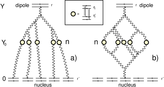
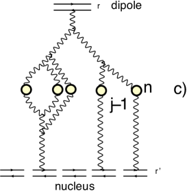
Figure 3: Summing large Pomeron loops for dipole-nucleus scattering. Fig. 3-a: the parton cascade of the fast dipole interacts with one dipole from the each parton cascade generated by the nucleons (j =n in Eq. (II.3)). Fig. 3-b: the parton cascade of the fast dipole interacts with the parton cascade generated by one nucleon in a nucleus (j =1 in Eq. (II.3)). Fig. 3-c: The main contribution for arbitrary values of $j$. The wavy lines denote the BFKL Pomeron exchanges. The circles denote the amplitude $\gamma$ in the Born approximation of perturbative QCD. A nucleus is viewed as the bag of dipoles with the size $r^{\prime}$.

In Eq. (33) $z_{i}$ is given in Eq. (18) while $z^{\prime}_{i}\,\,=\,\,\,\,\bar{\alpha}_{S}\frac{\chi\left(\bar{\gamma}\right)}{\bar{\gamma}}\left(Y_{0}\right)\,\,+\,\,\xi_{r^{\prime},r^{\prime}_{i}}$. $\xi_{r^{\prime},r^{\prime}_{i}}$ is equal to $\xi_{r,r_{i}}$ of Eq. (11) where $r$ and $r_{i}$ are replaced by $r^{\prime}$ and $r^{\prime}_{i}$, respectively.

Using Eq. (16) we reduce Eq. (33) to the following expression:

$$S\left(z^{\prime}\right)=S_{A}\left(b\right)C^{2}\sum^{\infty}_{n=0}\frac{\left(-1\right)^{n}}{n!}\!\!\!\int\limits^{\epsilon+i\infty}_{\epsilon-i\infty}\!\!\!\frac{d\omega}{2\,\pi\,i}\!\!\!\int\limits^{\epsilon+i\infty}_{\epsilon_{i}\infty}\!\!\!\frac{d\omega_{1}}{2\,\pi\,i}e^{\frac{\bar{\gamma}^{2}\kappa}{2}\left(\omega^{2}+\omega^{2}_{1}\right)}\frac{\Gamma\left(\omega+n\right)}{\Gamma\left(\omega\right)}\frac{\Gamma\left(\omega_{1}+n\right)}{\Gamma\left(\omega_{`}\right)}\left(\frac{G_{I\!\!P}\left(z^{\prime}\right)}{N_{0}}\right)^{n}$$ (33)

with

$$z^{\prime}\,\,=\,\,\,\,\bar{\alpha}_{S}\frac{\chi\left(\bar{\gamma}\right)}{\bar{\gamma}}\,Y\,\,+\,\,\xi_{r,r^{\prime}}$$ (34)

$\xi_{r,r^{\prime}}$ is equal to $\xi_{r,R}$ of Eq. (11) where $r$ and $R$ are replaced by $r$ and $r^{\prime}$, respectively.

Plugging Eq. (28) into Eq. (34) we obtain:

$$S\left(z^{\prime}\right)=C^{2}\,S_{A}\left(b\right)\sum^{\infty}_{n=0}\frac{\left(-1\right)^{n}}{n!}\!\!\!\int\limits^{\epsilon+i\infty}_{\epsilon-i\infty}\!\!\!\frac{d\omega}{2\,\pi\,i}\!\!\!\int\limits^{\epsilon+i\infty}_{\epsilon_{i}\infty}\!\!\!\frac{d\omega_{1}}{2\,\pi\,i}e^{\frac{\bar{\gamma}^{2}\kappa}{2}\left(\omega^{2}+\omega^{2}_{1}\right)}\int\limits^{\infty}_{0}dte^{-t}t^{\omega_{1}-1}\frac{\Gamma\left(\omega+n\right)}{\Gamma\left(\omega\right)\Gamma\left(\omega_{1}\right)}\left(t\,\frac{G_{I\!\!P}\left(z^{\prime}\right)}{N^{2}_{0}}\right)^{n}$$ (35)

After summation over $n$ we have

$$S\left(z^{\prime}\right) = C^{2}S_{A}\left(b\right)\int\limits^{\epsilon+i\infty}_{\epsilon-i\infty}\!\!\!\frac{d\omega}{2\,\pi\,i}\!\!\!\int\limits^{\epsilon+i\infty}_{\epsilon-i\infty}\!\!\!\frac{d\omega_{1}}{2\,\pi\,i}e^{\frac{\bar{\gamma}^{2}\kappa}{2}\left(\omega^{2}+\omega^{2}_{1}\right)}\frac{1}{\Gamma\left(\omega_{1}\right)}\int\limits^{\infty}_{0}dte^{-t}\left(1\,+\,t\frac{G_{I\!\!P}\left(z^{\prime}\right)}{N^{2}_{0}}\right)^{-\omega}\,t^{\omega_{1}-1}$$ (36)

$$= C^{2}S_{A}\left(b\right)\int\limits^{\epsilon+i\infty}_{\epsilon-i\infty}\!\!\!\frac{d\omega}{2\,\pi\,i}\!\!\!\int\limits^{\epsilon+i\infty}_{\epsilon-i\infty}\!\!\!\frac{d\omega_{1}}{2\,\pi\,i}e^{\frac{\bar{\gamma}^{2}\kappa}{2}\left(\omega^{2}+\omega^{2}_{1}\right)}\frac{1}{\Gamma\left(\omega_{1}\right)}\int\limits^{\infty}_{0}dte^{-t}\exp\left(-\omega\,\ln\left(\frac{G_{I\!\!P}\left(z^{\prime}\right)}{N^{2}_{0}}\right)\right)\,t^{\omega_{1}-\omega-1}$$

$$= C^{2}S_{A}\left(b\right)\int\limits^{\epsilon+i\infty}_{\epsilon-i\infty}\!\!\!\frac{d\omega}{2\,\pi\,i}\!\!\!\int\limits^{\epsilon+i\infty}_{\epsilon-i\infty}\!\!\!\frac{d\omega_{1}}{2\,\pi\,i}e^{\frac{\bar{\gamma}^{2}\kappa}{2}\left(\omega^{2}+\omega^{2}_{1}\right)}\frac{\Gamma\left(\omega_{1}-\omega\right)}{\Gamma\left(\omega_{1}\right)}\exp\left(-\omega\,\ln\left(\frac{G_{I\!\!P}\left(z^{\prime}\right)}{N^{2}_{0}}\right)\right)$$

Closing contour of integration over $\omega_{1}$ on the poles of $\Gamma\left(\omega-\omega_{1}\right)$ one can see that the main contribution gives the pole $\omega-\omega_{1}$ while all other poles lead to the amplitude that decreases as $\exp\left(-\bar{\gamma}\,n\,z^{\prime}\right)$ for the pole $\omega_{1}=\omega-n$. Taking integral over $\omega$ we obtain: The resulting $S\left(z^{\prime}\right)$ takes the form which has been found in Ref.LEDIDI :

$$S\left(z^{\prime}\right)=S_{A}\left(b\right)C^{\prime 2}\exp\left(-\frac{z^{\prime 2}}{4\kappa}\right)$$ (37)

Hence, we can conclude that the sum of the large Pomeron loops leads to the S-matrix in perfect agreement with the estimates of ’rare’ fluctuation, given in Ref.IAMU .

III.3 j = 2

Using Eq. (23b) for $\rho^{T}_{n}$ we can rewrite Eq. (1) in the form:

$$S_{A}\left(z\right)=\frac{1}{2}S^{2}_{A}\left(b\right)C^{2}\sum^{\infty}_{n=0}\frac{\left(-1\right)^{n}}{n!}\!\!\!\int\limits^{\epsilon+i\infty}_{\epsilon-i\infty}\!\!\!\frac{d\omega}{2\,\pi\,i}\!\!\!\int\limits^{\epsilon+i\infty}_{\epsilon_{i}\infty}\!\!\!\frac{d\omega_{1}}{2\,\pi\,i}\!\!\int\limits^{\epsilon+i\infty}_{\epsilon_{i}\infty}\!\!\!\frac{d\omega_{2}}{2\,\pi\,i}e^{\frac{\bar{\gamma}^{2}\kappa}{2}\left(\omega^{2}+\omega_{1}^{2}+\omega^{2}_{2}\right)}\frac{\Gamma\left(\omega+n\right)}{\Gamma\left(\omega\right)}$$

$$\sum_{k=1}^{n-1}\frac{n!}{k!(n-k)!}\frac{\Gamma\left(\omega_{1}+k\right)}{\Gamma\left(\omega_{1}\right)}\frac{\Gamma\left(\omega_{2}+n-k\right)}{\Gamma\left(\omega_{2}\right)}\int\limits\!\!\!d^{2}r_{i}d^{2}r^{\prime}_{i}d^{2}b_{i}d^{2}b^{\prime}_{i}\prod^{n}_{i=1}\frac{G_{I\!\!P}\left(z_{i}\right)}{N_{0}}\gamma^{BA}\left(r_{i},r^{\prime}_{i},\delta b\right)\frac{G_{I\!\!P}\left(z^{\prime}_{i}\right)}{N_{0}}$$ (38)

From Eq. (16) and replacing $\Gamma$ functions by the integrals over $t_{i}$ (see Eq. (28)) we obtain

$$S_{A}\left(z\right) = \frac{1}{2}S^{2}_{A}\left(b\right)C\sum^{\infty}_{n=0}\left(\frac{G_{I\!\!P}\left(z^{\prime}\right)}{N_{0}}\right)^{n}\frac{(-1)^{n}}{n!}\!\!\!\int\limits^{\epsilon+i\infty}_{\epsilon-i\infty}\!\!\!\frac{d\omega}{2\,\pi\,i}\!\!\!\int\limits^{\epsilon+i\infty}_{\epsilon_{i}\infty}\!\!\!\frac{d\omega_{1}}{2\,\pi\,i}\!\!\int\limits^{\epsilon+i\infty}_{\epsilon_{i}\infty}\!\!\!\frac{d\omega_{2}}{2\,\pi\,i}e^{\frac{\bar{\gamma}^{2}\kappa}{2}\left(\omega^{2}+\omega^{2}+\omega^{2}_{1}\right)}\frac{\Gamma\left(\omega+n\right)}{\Gamma\left(\omega\right)\Gamma\left(\omega_{1}\right)\Gamma\left(\omega_{2}\right)}$$ (39)

$$\int^{\infty}_{0}dt_{1}\int^{\infty}_{0}dt_{2}e^{-t_{1}-t_{2}}\underbrace{\sum_{k=1}^{n-1}\frac{n!}{k!\,(n-k)!}t_{1}^{\omega_{1}+k-1}t_{2}^{\omega_{1}+n-k-1}}_{(t_{1}+t_{2})^{n}-t_{1}^{n}-t_{2}^{n}}$$

Summing over $n$ we obtain:

$$S_{A}\left(z\right) = \frac{1}{2}S^{2}_{A}\left(b\right)C\sum^{\infty}_{n=0}\!\!\!\int\limits^{\epsilon+i\infty}_{\epsilon-i\infty}\!\!\!\frac{d\omega}{2\,\pi\,i}\!\!\!\int\limits^{\epsilon+i\infty}_{\epsilon_{i}\infty}\!\!\!\frac{d\omega_{1}}{2\,\pi\,i}\!\!\int\limits^{\epsilon+i\infty}_{\epsilon_{i}\infty}\!\!\!\frac{d\omega_{2}}{2\,\pi\,i}\!\!\int\limits^{\epsilon+i\infty}_{\epsilon_{i}\infty}\!\!\!\frac{d\omega_{2}}{2\,\pi\,i}e^{\frac{\bar{\gamma}^{2}\kappa}{2}\left(\omega^{2}+\omega_{1}^{2}+\omega^{2}_{2}+\omega^{2}_{3}\right)}\frac{1}{\Gamma\left(\omega_{1}\right)\Gamma\left(\omega_{2}\right)\Gamma\left(\omega_{3}\right)}\exp\left(-\omega\,\ln\left(\frac{G_{I\!\!P}\left(z^{\prime}\right)}{N_{0}}\right)\right)$$ (40)

$$\int\limits^{\infty}_{0}\!\!\!dt_{1}\!\!\int\limits^{\infty}_{0}\!\!\!dt_{2}\,\,e^{-t_{1}-t_{2}}\,\Bigg{\{}t_{1}^{\omega_{1}-1}\,t_{2}^{\omega_{2}-1}\left(t_{1}+t_{2}\right)^{-\omega}-\,t_{1}^{\omega_{1}-\omega-1}\,t_{2}^{\omega-1}-\,t_{2}^{\omega_{2}-\omega-1}\,t_{1}^{\omega_{2}-1}\Bigg{\}}$$

Taking integrals over $t_{1}$ and $t_{2}$ we reduce Eq. (40) to the form:

$$S_{A}\left(z\right) = \frac{1}{2}S^{2}_{A}\left(b\right)C\!\!\!\int\limits^{\epsilon+i\infty}_{\epsilon-i\infty}\!\!\!\frac{d\omega}{2\,\pi\,i}\!\!\!\int\limits^{\epsilon+i\infty}_{\epsilon_{i}\infty}\!\!\!\frac{d\omega_{1}}{2\,\pi\,i}\!\!\int\limits^{\epsilon+i\infty}_{\epsilon_{i}\infty}\!\!\!\frac{d\omega_{2}}{2\,\pi\,i}e^{\frac{\bar{\gamma}^{2}\kappa}{2}\left(\omega^{2}+\omega_{1}^{2}+\omega^{2}_{2}\right)}\exp\left(-\omega\,\ln\left(\frac{G_{I\!\!P}\left(z^{\prime}\right)}{N_{0}}\right)\right)\,$$ (41a)

$$\Bigg{\{}\underbrace{\frac{\Gamma\left(\omega_{1}+\omega_{2}-\omega\right)}{\Gamma\left(\omega_{1}+\omega_{2}\right)}}_{\rm I}\,-\,\underbrace{\frac{\Gamma\left(\omega_{1}-\omega\right)}{\Gamma\left(\omega_{1}\right)}}_{\rm II}\,-\,\underbrace{\frac{\Gamma\left(\omega_{2}-\omega\right)}{\Gamma\left(\omega_{2}\right)}}_{\rm III}\Bigg{\}}$$

$$= \frac{1}{2}S^{2}_{A}\left(b\right)C\Bigg{\{}\underbrace{C^{\prime}\exp\left(-\frac{z^{\prime 2}}{3\kappa}\right)}_{\rm I}\,\,-\,\,\underbrace{C^{\prime}\exp\left(-\frac{z^{\prime 2}}{4\kappa}\right)}_{\rm II}\,-\,\,\underbrace{C^{\prime}\exp\left(-\frac{z^{\prime 2}}{4\kappa}\right)}_{\rm III}\Bigg{\}}$$ (41b)

$$\xrightarrow{z\gg 1} -S^{2}_{A}\left(b\right)C^{\prime}\exp\left(-\frac{z^{\prime 2}}{4\kappa}\right)$$ (41c)

III.4 j = 3

From Eq. (1) the scattering amplitude in this case is equal to:

$$S_{A}\left(z\right)=\frac{1}{3!}S^{3}_{A}\left(b\right)C^{3}\sum^{\infty}_{n=0}\frac{\left(-1\right)^{n}}{n!}\!\!\!\int\limits^{\epsilon+i\infty}_{\epsilon-i\infty}\!\!\!\frac{d\omega}{2\,\pi\,i}e^{\frac{\bar{\gamma}^{2}\kappa}{2}\omega^{2}}\frac{\Gamma\left(\omega+n\right)}{\Gamma\left(\omega\right)}\prod^{3}_{i=1}\!\!\int\limits^{\epsilon+i\infty}_{\epsilon_{i}\infty}\!\!\!\frac{d\omega_{i}}{2\,\pi\,i}e^{\frac{\bar{\gamma}^{2}\kappa}{2}\omega_{i}^{2}}\,\sum_{k_{i}=1}^{n-2}\frac{n!}{k_{1}!k_{2}!(n-k_{1}-k_{2})!}$$

$$\frac{\Gamma\left(\omega_{1}+k_{1}\right)}{\Gamma\left(\omega_{1}\right)}\frac{\Gamma\left(\omega_{2}+k_{2}\right)}{\Gamma\left(\omega_{2}\right)}\frac{\Gamma\left(\omega_{3}+n-k_{1}-k_{2}\right)}{\Gamma\left(\omega_{3}\right)}\int\limits\!\!\!d^{2}r_{i}d^{2}r^{\prime}_{i}d^{2}b_{i}d^{2}b^{\prime}_{i}\prod^{n}_{i=1}\frac{G_{I\!\!P}\left(z_{i}\right)}{N_{0}}\gamma^{BA}\left(r_{i},r^{\prime}_{i},\delta b\right)\frac{G_{I\!\!P}\left(z^{\prime}_{i}\right)}{N_{0}}$$ (42)

Using Eq. (16) and Eq. (28) we obtain:

$$S_{A}\left(z\right) = \frac{1}{3!}S^{3}_{A}\left(b\right)C^{3}\sum^{\infty}_{n=0}\frac{\left(-1\right)^{n}}{n!}\!\!\!\left(\frac{G_{I\!\!P}\left(z^{\prime}\right)}{N_{0}}\right)^{n}\int\limits^{\epsilon+i\infty}_{\epsilon-i\infty}\!\!\!\frac{d\omega}{2\,\pi\,i}e^{\frac{\bar{\gamma}^{2}\kappa}{2}\omega^{2}}\frac{\Gamma\left(\omega+n\right)}{\Gamma\left(\omega\right)}\prod^{3}_{i=1}\!\!\int\limits^{\epsilon+i\infty}_{\epsilon_{i}\infty}\!\!\!\frac{d\omega_{i}}{2\,\pi\,i}\frac{1}{\Gamma\left(\omega_{i}\right)}e^{\frac{\bar{\gamma}^{2}\kappa}{2}\omega_{i}^{2}}\,\int\limits^{\infty}_{0}dt_{i}e^{-t_{i}}t_{i}^{\omega_{i}-1}$$ (43)

$$\underbrace{\sum_{k=1}^{n-1}\frac{n!}{k_{1}!k_{2}!(n-k_{1}-k_{2})!}t_{1}^{k_{1}}t_{2}^{k_{2}}t_{3}^{n-k_{1}-k_{2}}}_{t_{1}^{n}+t_{2}^{n}+t_{3}^{n}-(t_{1}+t_{2})^{n}-(t_{1}+t_{3})^{n}-(t_{2}+t_{3})^{n}+(t_{1}+t_{2}+t_{3})^{n}}$$

After summation over $n$ we have

$$S_{A}\left(z\right) = \frac{1}{3!}S^{3}_{A}\left(b\right)C^{3}\!\!\!\int\limits^{\epsilon+i\infty}_{\epsilon-i\infty}\!\!\!\frac{d\omega}{2\,\pi\,i}e^{\frac{\bar{\gamma}^{2}\kappa}{2}\omega^{2}}\prod^{3}_{i=1}\int\limits^{\epsilon+i\infty}_{\epsilon_{i}\infty}\!\!\!\frac{d\omega_{i}}{2\,\pi\,i}e^{\frac{\bar{\gamma}^{2}\kappa}{2}\omega_{i}^{2}}\frac{1}{\Gamma\left(\omega_{i}\right)}\exp\left(-\omega\,\ln\left(\frac{G_{I\!\!P}\left(z^{\prime}\right)}{N_{0}}\right)\right)$$

$$\int\limits^{\infty}_{0}\!\!\!dt_{1}\!\!\int\limits^{\infty}_{0}\!\!\!dt_{2}\!\!\int\limits^{\infty}_{0}\!\!\!dt_{3}e^{-t_{1}-t_{2}-t_{3}}\,\Bigg{\{}t_{1}^{-\omega}+t_{2}^{-\omega}+t_{3}^{-\omega}-(t_{1}+t_{2})^{-\omega}-(t_{1}+t_{3})^{-\omega}-(t_{2}+t_{3})^{-\omega}+(t_{1}+t_{2}+t_{3})^{-\omega}\Bigg{\}}$$

Taking integrals over $t_{i}$ we obtain:

$$S_{A}\left(z\right) = \frac{1}{3!}S^{3}_{A}\left(b\right)C^{3}\!\!\!\int\limits^{\epsilon+i\infty}_{\epsilon-i\infty}\!\!\!\frac{d\omega}{2\,\pi\,i}e^{\frac{\bar{\gamma}^{2}\kappa}{2}\omega^{2}}\prod^{3}_{i=1}\int\limits^{\epsilon+i\infty}_{\epsilon_{i}\infty}\!\!\!\frac{d\omega_{i}}{2\,\pi\,i}e^{\frac{\bar{\gamma}^{2}\kappa}{2}\omega_{i}^{2}}\exp\left(-\omega\,\ln\left(\frac{G_{I\!\!P}\left(z^{\prime}\right)}{N_{0}}\right)\right)$$

$$\,\Bigg{\{}\underbrace{\sum^{3}_{i=1}\frac{\Gamma\left(\omega_{i}-\omega\right)}{\Gamma\left(\omega_{i}\right)}}_{\rm I}-\underbrace{\frac{\Gamma\left(\omega_{1}+\omega_{2}-\omega\right)}{\Gamma\left(\omega_{1}+\omega_{2}\right)}-\frac{\Gamma\left(\omega_{1}+\omega_{3}-\omega\right)}{\Gamma\left(\omega_{1}+\omega_{3}\right)}-\frac{\Gamma\left(\omega_{2}+\omega_{3}-\omega\right)}{\Gamma\left(\omega_{2}+\omega_{3}\right)}}_{\rm II}+\underbrace{\frac{\Gamma\left(\omega_{1}+\omega_{2}+\omega_{3}-\omega\right)}{\Gamma\left(\omega_{1}+\omega_{2}+\omega_{3}\right)}\Bigg{\}}}_{\rm III}$$

$$= \frac{1}{3!}S^{3}_{A}\left(b\right)C^{3}\Bigg{\{}\underbrace{3\,C^{\prime}\exp\left(-\frac{z^{\prime 2}}{4\kappa}\right)}_{\rm I}-3\underbrace{C^{\prime}\exp\left(-\frac{z^{\prime 2}}{3\kappa}\right)}_{\rm II}\,+\,\underbrace{C^{\prime}\exp\left(-\frac{3z^{\prime 2}}{8\kappa}\right)}_{\rm III}\Bigg{\}}$$ (45b)

$$\xrightarrow{z\gg 1} -\frac{1}{2}S^{3}_{A}\left(b\right)C^{\prime}\exp\left(-\frac{z^{\prime 2}}{4\kappa}\right)$$ (45c)

Eq. (45b) is derived from Eq. (45) performing integration over $\omega$ closing contour on the poles of $\Gamma$ functions.

III.5 General case

The scattering amplitude in the general case of arbitrary $j$ can be written as follows:

$$S_{A}\left(z\right) = \frac{(-1)^{j+1}}{j!}S^{j}_{A}\left(b\right)C^{j}\!\!\!\int\limits^{\epsilon+i\infty}_{\epsilon-i\infty}\!\!\!\frac{d\omega}{2\,\pi\,i}e^{\frac{\bar{\gamma}^{2}\kappa}{2}\omega^{2}}\prod^{j}_{i=1}\int\limits^{\epsilon+i\infty}_{\epsilon_{i}\infty}\!\!\!\frac{d\omega_{i}}{2\,\pi\,i}e^{\frac{\bar{\gamma}^{2}\kappa}{2}\omega_{i}^{2}}\exp\left(-\omega\,\ln\left(\frac{G_{I\!\!P}\left(z^{\prime}\right)}{N_{0}}\right)\right)$$

$$\sum^{j}_{j^{\prime}=1}(-1)^{j^{\prime}+1}\frac{j!}{j^{\prime}!\,(j-j^{\prime})!}\frac{\Gamma\left(\sum_{i=1}^{j^{\prime}}\omega_{i}\,-\,\omega\right)}{\Gamma\left(\sum_{i=1}^{j^{\prime}}\omega_{i}\right)}$$

We close the contour of integration on the pole $\sum_{i=1}^{j^{\prime}}\omega_{i}\,-\,\omega=0$ reducing the term with $j^{\prime}$ in $N_{A}\left(z\right)(N^{j^{\prime}}_{A}\left(z\right))$ to the form:

$$S^{j^{\prime}}_{A}\left(z\right)=\frac{(-1)^{j+1}}{j!}S^{j}_{A}\left(b\right)C^{j}\!\!\!\int\limits^{\epsilon+i\infty}_{\epsilon-i\infty}\!\!\!\frac{d\omega}{2\,\pi\,i}\prod^{j}_{i=2}\int\limits^{\epsilon+i\infty}_{\epsilon_{i}\infty}\!\!\!\frac{d\omega_{i}}{2\,\pi\,i}e^{\frac{1}{2}\bar{\gamma}^{2}\kappa\left(\omega^{2}+\left(\omega-\sum_{i=2}^{j^{\prime}}\omega_{i}\right)^{2}+\sum_{i=2}^{j^{\prime}}\omega_{i}^{2}\right)}\exp\left(-\omega\,\ln\left(\frac{G_{I\!\!P}\left(z^{\prime}\right)}{N_{0}}\right)\right)$$ (47)

Expecting that $\omega\propto\,\bar{\gamma}z$ is large we can take the integrals over $\omega$’s using the method of steepest descent . The equations for the saddle points are the following:

$$(1)\,\,\,\bar{\gamma}^{2}\kappa\left(2\omega^{\mbox{\tiny SP}}-\sum_{i=2}^{j^{\prime}}\omega^{\mbox{\tiny SP}}_{i}\right)-\bar{\gamma}z\,=\,0\,;~~~~~(i)\,\,\,\omega^{\mbox{\tiny SP}}_{i}\,+\,\sum_{i=2}^{j^{\prime}}\omega^{\mbox{\tiny SP}}_{i}\,-\,\omega\,=\,0\,;$$ (48)

Solutions to these equations are $\omega^{\mbox{\tiny SP}}_{i}=\frac{1}{j^{\prime}}\omega$ and $\omega^{\mbox{\tiny SP}}\,\,=\,\,\frac{j^{\prime}}{j^{\prime}+1}\frac{z}{\bar{\gamma}\,\kappa}$. Using these solutions we obtain for the scattering amplitude:

$$S_{A}\left(z\right) = \frac{(-1)^{j+1}}{j!}S^{j}_{A}\left(b\right)C^{j}\,\sum^{j}_{j^{\prime}=1}(-1)^{j^{\prime}+1}\frac{j!}{j^{\prime}!\,(j-j^{\prime})!}C^{\prime}\exp\left(-\frac{j^{\prime}}{j^{\prime}+1}\frac{z^{\prime 2}}{2\kappa}\right)$$ (49a)

$$\xrightarrow{z\gg 1} \,\,\frac{(-1)^{j+1}}{(j-1)!}S^{j}_{A}\left(b\right)C^{j}\,\exp\left(-\frac{z^{\prime 2}}{4\kappa}\right)$$ (49b)

From Eq. (49a) one can see that the main contribution stems from $j^{\prime}=1$ which corresponds to the configuration shown in Fig. 3-c, viz.: $j-1$ nucleons deliver one dipole each to the rapidity $Y_{0}$ . The solution to BK equation leads to the asymptotic behaviour of the last term in the sum of Eq. (49a) $j^{\prime}=j$ for large value of $j$.

In principle we cannot sum Eq. (49b) over $j$. However, assuming that the smooth function is equal to $C^{j}$ as it is shown ion Eq. (49b) we c an obtain the scattering amplitude in the fortm

$$S_{A}\left(z;b\right)\,\,=\,\,C\,S_{A}\left(b\right)\exp\left(-C\,S_{A}\left(b\right)\right)\exp\left(-\frac{z^{\prime 2}}{4\kappa}\right)$$ (50)

The integral over $b$ can be taken in two limited models: $S_{A}$ has a Gaussian form or $S_{A}$ is a cylinder of radius $R_{A}$, The result is

Gaussian model: $$S_{A}\left(z;b\right)\,\,=\,\,\pi\,R^{2}_{A}\left(1-\exp\left(-C\,\frac{A}{\pi R^{2}_{A}}\right)\right)\exp\left(-\frac{z^{\prime 2}}{4\kappa}\right);$$

Cylindrical model: $$S_{A}\left(z;b\right)\,\,=\,\,C\,A\exp\left(-C\frac{A}{\pi R^{2}_{A}}\right)\,\,\exp\left(-\frac{z^{\prime 2}}{4\kappa}\right);$$ (51)

where $C$ has dimension of the cross section.

Comparing Eq. (III.5) with the BK amplitude at large $z$:

$$S^{BK}_{A}\left(z\right)\,=\,\pi R^{2}_{A}\,C\exp\left(-\frac{z^{\prime 2}}{2\kappa}\right)$$ (52)

one can see that for $z\,>\,\sqrt{2\,\kappa\,C}A^{1/6}$ the BK equation gives the scattering amplitude which is smaller than the one which stems from the large Pomeron loops.

IV Conclusions

In this paper we summed the large BFKL Pomeron loops in the framework of the BFKL Pomeron calculus for the scattering of dipole with nucleus target.The main result is that this scattering amplitude has the same energy dependence as the dipole-dipole amplitude. It means that the non-linear BK equation cannot describe the contribution of the large Pomeron loops and can only be used in the limited range of energy for the dipole-nucleus scattering: $z\,\leq\,\sqrt{2\,\kappa\,C}A^{1/6}$

The result has been expected since it is shown in Refs.KLLL1 ; KLLL2 that BK equation violates the s-channel unitarity. The kind of surprise is the resulting scattering amplitude coincides with the dipole-dipole scattering at high energy.

We hope that this paper will contribute to the further study of the Pomeron calculus in QCD.

Acknowledgements

We thank our colleagues at Tel Aviv university for discussions. Special thanks go A. Kovner and M. Lublinsky for stimulating and encouraging discussions on the subject of this paper. This research was supported by BSF grant 2022132.

Appendix A Useful formulae for $\rho^{T}_{n}\left(r,b,\{r_{i},b_{i}\}\right)$

One can check that

$$\frac{1}{k_{i}!}\frac{\Gamma\left(\omega_{i}+k_{i}\right)}{\Gamma\left(\omega_{i}\right)}\,=\,\frac{\sin\left(\pi\omega_{i}\right)}{\pi}\int^{1}_{0}dt_{i}\left(\frac{t_{i}}{1-t_{i}}\right)^{\omega_{i}}t_{i}^{k_{i}-1}$$ (53)

Plugging this equation in Eq. (27) we have

$$\rho^{T}_{n}\left(r,b,\{r_{i},b_{i}\}\right)\,\, = \,\,\prod^{n}_{i=1}\frac{G_{I\!\!P}\left(z_{i}\right)}{N_{0}}\sum^{n}_{j=1}\frac{1}{j!}S^{j}_{A}\left(b\right)\!\!\!\!\!\!\!\!\!\!\!\!\!\!\!\sum^{k_{1}=n-j+1,\dot{\,}k_{j}=n-j+1}_{k_{1}=1,\dot{\,}k_{j}=1}\!\!\!\!\!\!\!\!\!\!\!\!\!\!\!\!\!\!\!\!\delta_{\sum_{i=1}^{j}k_{i}=n}$$ (54)

$$\times \prod^{j}_{i=1}C\,\int\limits^{\epsilon+i\infty}_{\epsilon-i\infty}\frac{d\omega_{i}}{2\,\pi\,i}\int^{1}_{0}dt_{i}e^{\frac{\bar{\gamma}\,\kappa}{2}\,\omega_{i}^{2}}\frac{\sin\left(\pi\omega_{i}\right)}{\pi}\left(\frac{t_{i}}{1-t_{i}}\right)^{\omega_{i}}t_{i}^{k_{i}-1}$$

Replacing $\delta_{\sum_{i=1}^{j}k_{i}=n}$ by

$$\delta_{\sum_{i=1}^{j}k_{i}=n}\,\,=\,\,\oint_{C}\mu^{n-\sum^{j}_{i=1}k_{i}-1}d\mu$$ (55)

with contour C being the circle around $\mu=0$, we obtain the following $\rho^{T}_{n}\left(r,b,\{r_{i},b_{i}\}\right)$ after summing over $k_{i}$:

$$\rho^{T}_{n}\left(r,b,\{r_{i},b_{i}\}\right)\,\, = \,\,\prod^{n}_{i=1}\frac{G_{I\!\!P}\left(z_{i}\right)}{N_{0}}\sum^{n}_{j=1}\frac{1}{j!}S^{j}_{A}\left(b\right)\oint_{C}\mu^{n-1}d\mu$$ (56)

$$\times \prod^{j}_{i=1}C\,\int\limits^{\epsilon+i\infty}_{\epsilon-i\infty}\frac{d\omega_{i}}{2\,\pi\,i}\int^{1}_{0}dt_{i}e^{\frac{\bar{\gamma}\,\kappa}{2}\,\omega_{i}^{2}}\frac{\sin\left(\pi\omega_{i}\right)}{\pi}\left(\frac{t_{i}}{1-t_{i}}\right)^{\omega_{i}}\frac{1}{\mu}\frac{1-\left(\frac{t_{i}}{\mu}\right)^{n-j+1}}{1-\left(\frac{t_{i}}{\mu}\right)}$$

Taking integrals over $t_{i}$ we have:

$$\rho^{T}_{n}\left(r,b,\{r_{i},b_{i}\}\right)\,\, = \,\,\prod^{n}_{i=1}\frac{G_{I\!\!P}\left(z_{i}\right)}{N_{0}}\sum^{n}_{j=1}\frac{1}{j!}S^{j}_{A}\left(b\right)\oint_{C}\mu^{n-1}d\mu\prod^{j}_{i=1}C\,\int\limits^{\epsilon+i\infty}_{\epsilon-i\infty}\frac{d\omega_{i}}{2\,\pi\,i}e^{\frac{\bar{\gamma}\,\kappa}{2}\,\omega_{i}^{2}}\Bigg{\{}\left((\mu-1)^{-\omega}\mu^{\omega}-1\right)$$ (57)

$$- \sin\left(\pi\omega_{i}\right)\Gamma(1-\omega)\left(\frac{1}{\mu}\right)^{-j+n+2}\!\!\!\!\!\!\!\!\!\!\!\!\!\!\Gamma(-j+n+\omega+2)\,_{2}\tilde{F}_{1}\left(1,-j+n+\omega+2;-j+n+3;\frac{1}{\mu}\right)\Bigg{\}}$$

References

• (1) V. S. Fadin, E. A. Kuraev and L. N. Lipatov, Phys. Lett. B60, 50 (1975);    E. A. Kuraev, L. N. Lipatov and V. S. Fadin, Sov. Phys. JETP 45, 199 (1977), [Zh. Eksp. Teor. Fiz.72,377(1977)];    I. I. Balitsky and L. N. Lipatov, Sov. J. Nucl. Phys. 28, 822 (1978), [Yad. Fiz.28,1597(1978)].
• (2) L. V. Gribov, E. M. Levin and M. G. Ryskin, Phys. Rept.  100, 1 (1983).
• (3) E. M. Levin and M. G. Ryskin, Phys. Rept.  189, 267 (1990).
• (4) A. H. Mueller and J. Qiu, Nucl. Phys. B268 (1986) 427.
• (5) A. H. Mueller, Nucl. Phys. B 415 (1994) 373;    Nucl. Phys. B 437 (1995) 107, [hep-ph/9408245]
A. H. Mueller and B. Patel, Nucl. Phys. B 425, 471, 1994.
• (6) I. Balitsky, Phys. Rev. D60, 014020 (1999),[arXiv:hep-ph/9812311];
• (7) Y. V. Kovchegov, Phys. Rev. D60, 034008 (1999),[arXiv:hep-ph/9901281].
• (8) J. Bartels, Z. Phys. C 60 (1993), 471-488 ;   J. Bartels and M. Wusthoff, Z. Phys. C 66 (1995), 157-1801;    J. Bartels and C. Ewerz, JHEP 09 (1999), 026 [arXiv:hep-ph/9908454];   C. Ewerz, JHEP 0104 (2001) 031, [hep-ph/0103260].
• (9) M. A. Braun, Phys. Lett. B 483, 115 (2000), [hep-ph/0003004]; Eur. Phys. J. C 33, 113 (2004),[hep-ph/0309293];Phys. Lett. B 632, 297 (2006).
• (10) M. A. Braun, Eur. Phys. J. C16 (2000) 337, [arXiv:hep-ph/0001268];
M. A. Braun and G. P. Vacca, Eur. Phys. J. C6 (1999) 147,[arXiv:hep-ph/9711486];
J. Bartels, M. Braun and G. P. Vacca, Eur. Phys. J. C 40, 419 (2005), [arXiv:hep-ph/0412218],
J. Bartels, L. N. Lipatov and G. P. Vacca, Nucl. Phys. B 706, 391 (2005), [arXiv:hep-ph/0404110].
• (11) L. McLerran and R. Venugopalan, Phys. Rev. D49 (1994) 2233, Phys. Rev. D49 (1994), 3352; D50 (1994) 2225; D59 (1999) 09400.
• (12) J. Jalilian-Marian, A. Kovner, A. Leonidov and H. Weigert , Nucl. Phys. B504 (1997) 415–431, [ arXiv:hep-ph/9701284].
• (13) J. Jalilian-Marian, A. Kovner, A. Leonidov and H. Weigert , Phys.Rev. D59 (1998) 014014, [arXiv:hep-ph/9706377 [hep-ph]].
• (14) A. Kovner, J. G. Milhano and H. Weigert , Phys. Rev. D62 (2000) 114005, [ arXiv:hep-ph/0004014].
• (15) E. Iancu, A. Leonidov and L. D. McLerran ,Nucl. Phys. A692 (2001) 583–645, [ arXiv:hep-ph/0011241].
• (16) E. Iancu, A. Leonidov and L. D. McLerran , Phys. Lett. B510 (2001) 133–144, [ arXiv:hep-ph/0102009].
• (17) E. Ferreiro, E. Iancu, A. Leonidov and L. McLerran , Nucl. Phys. A703 (2002) 489–538, [ arXiv:hep-ph/0109115].
• (18) H. Weigert, Nucl. Phys. A 703 (2002), 823-860 [arXiv:hep-ph/0004044 [hep-ph]].
• (19) A. Kovner and J. G. Milhano, Phys. Rev. D 61 (2000), 014012 [arXiv:hep-ph/9904420 [hep-ph]].
• (20) E. Levin and M. Lublinsky, Nucl. Phys. A 730 (2004), 191-211,[hep-ph/0308279 [hep-ph];   Phys. Lett. B 607 (2005) 131, [hep-ph/0411121 [hep-ph]]
• (21) Yuri V. Kovchegov and Eugene Levin, “ Quantum Chromodynamics at High Energies", Cambridge Monographs on Particle Physics, Nuclear Physics and Cosmology, Cambridge University Press, 2012 .
• (22) A. Kovner, E. Levin, M. Li and M. Lublinsky, JHEP 09 (2020), 199 [arXiv:2006.15126 [hep-ph]].
• (23) A. Kovner, E. Levin, M. Li and M. Lublinsky, JHEP 10 (2020), 185 [arXiv:2007.12132 [hep-ph]].
• (24) A. H. Mueller and G. P. Salam, Nucl. Phys. B 475, 293 (1996), [hep-ph/9605302];   G. P. Salam, Nucl. Phys. B 461, 512 (1996), [hep-ph/9509353].
• (25) E. Levin and K. Tuchin, Nucl. Phys. B 573, 833 (2000) [hep-ph/9908317];    Nucl. Phys. A 691, 779 (2001) [hep-ph/0012167]; 693, 787 (2001) [hep-ph/0101275].
• (26) E. Levin and M. Lublinsky, Nucl. Phys. A 763 (2005) 172, [hep-ph/0501173 [hep-ph]].
• (27) L. N. Lipatov, Sov. Phys. JETP 63, 904 (1986) [Zh. Eksp. Teor. Fiz.  90, 1536 (1986)].
• (28) Y. V. Kovchegov, Phys. Rev. D 72 (2005), 094009, [arXiv:hep-ph/0508276].
• (29) P. Rembiesa and A. M. Stasto, Nucl. Phys. B 725 (2005) 251, [hep-ph/0503223].
• (30) A. Kovner and M. Lublinsky, Nucl. Phys. A 767 171 (2006), [hep-ph/0510047].
• (31) A. I. Shoshi and B. W. Xiao, Phys. Rev. D 73 (2006) 094014, [hep-ph/0512206].
• (32) M. Kozlov and E. Levin, Nucl. Phys. A 779 (2006) 142, [hep-ph/0604039].
• (33) N. Armesto, S. Bondarenko, J. G. Milhano and P. Quiroga, JHEP 0805 (2008) 103, arXiv:0803.0820 [hep-ph].
• (34) E. Levin and A. Prygarin, Eur. Phys. J. C 53 (2008) 385, [hep-ph/0701178].
• (35) A. D. Le, A. H. Mueller and S. Munier, Phys. Rev. D 104, 034026 (2021), [arXiv:2103.10088 [hep-ph]].
• (36) E. Levin, Phys. Rev. D 104, no.5, 056025 (2021), [arXiv:2106.06967 [hep-ph]].
• (37) A. H. Mueller and D. N. Triantafyllopoulos, Nucl. Phys. B 640 (2002) 331, [hep-ph/0205167]
• (38) S. Munier and R. B. Peschanski, Phys. Rev. D 69 (2004), 034008 doi:10.1103/PhysRevD.69.034008 [arXiv:hep-ph/0310357 [hep-ph]]; Phys. Rev. Lett. 91 (2003), 232001 doi:10.1103/PhysRevLett.91.232001 [arXiv:hep-ph/0309177 [hep-ph]].
• (39) E. Iancu, K. Itakura and L. McLerran, Nucl. Phys. A 708 (2002) 327, [hep-ph/0203137].
• (40) L. N. Lipatov, Phys. Rept.  286 (1997) 131, [hep-ph/9610276].
• (41) L. N. Lipatov, Nucl. Phys. B 365, 614 (1991), Nucl. Phys. B 452, 369 (1995), [arXiv:hep-ph/9502308];
R. Kirschner, L. N. Lipatov and L. Szymanowski, Nucl. Phys. B 425, 579 (1994), [arXiv:hep-th/9402010]; Phys. Rev. D 51, 838 (1995), [arXiv:hep-th/9403082].
• (42) G. P. Salam, Nucl. Phys. B 461, 512 (1996); [hep-ph/9509353].
• (43) H. Navelet and R. B. Peschanski, Nucl. Phys. B 507 (1997), 353-366 [arXiv:hep-ph/9703238].
• (44) J. Bartels, Nucl. Phys.  B175, 365 (1980);
J. Kwiecinski and M. Praszalowicz, Phys. Lett.  B94, 413 (1980).
• (45) Y. V. Kovchegov and E. Levin, Nucl. Phys. B 577 (2000) 221, [hep-ph/9911523].
• (46) A. Kovner and M. Lublinsky, JHEP 02 (2007), 058, [arXiv:hep-ph/0512316 [hep-ph]].
• (47) T. Altinoluk, A. Kovner, E. Levin and M. Lublinsky, JHEP 04 (2014), 075 [arXiv:1401.7431 [hep-ph]].
• (48) A. Kovner and M. Lublinsky, Phys. Rev. D 71 (2005), 085004 [arXiv:hep-ph/0501198 [hep-ph]].
• (49) A. Kovner and M. Lublinsky, Phys. Rev. Lett.  94, 181603 (2005), [hep-ph/0502119].
• (50) I. Balitsky, Phys. Rev. D 72, 074027 (2005), arXiv:hep-ph/0507237.
• (51) Y. Hatta, E. Iancu, L. McLerran, A. Stasto and D. N. Triantafyllopoulos, Nucl. Phys. A 764, 423 (2006),[arXiv:hep-ph/0504182].
• (52) A. Kovner, M. Lublinsky and U. Wiedemann, JHEP 06 (2007), 075 [arXiv:0705.1713 [hep-ph]];    T. Altinoluk, A. Kovner, M. Lublinsky and J. Peressutti, JHEP 0903, 109 (2009), [arXiv:0901.2559 [hep-ph]].
• (53) A. Kovner and M. Lublinsky Nucl. Phys. A 767, 171-188 (2006),[arXiv:hep-ph/0510047].
• (54) A. Kormilitzin, E. Levin and A. Prygarin, Nucl. Phys. A 813 (2008), 1-13 [arXiv:0807.3413 [hep-ph]];    E. Levin and A. Prygarin, Eur. Phys. J. C 53 (2008), 385-399 [arXiv:hep-ph/0701178 [hep-ph]].
• (55) E. Levin, Phys. Rev. D 107 (2023) no.5, 054012 [arXiv:2209.07095 [hep-ph]].
• (56) E. Levin, “Scattering amplitude in QCD: summing large Pomeron loops,” [arXiv:2403.10364 [hep-ph]].
• (57) E. Levin, Nucl. Phys. A 763 (2005), 140-171, [arXiv:hep-ph/0502243 [hep-ph]].
• (58) E. Levin, Phys. Rev. D 110, no.11, 116021 (2024), [arXiv:2409.00761 [hep-ph]].
• (59) J. Bartels, E. Levin, Nucl. Phys.  B387 (1992) 617-637;   A. M. Stasto, K. J. Golec-Biernat, J. Kwiecinski, Phys. Rev. Lett.  86 (2001) 596-599, [hep-ph/0007192];   L. McLerran, M. Praszalowicz, Acta Phys. Polon.  B42 (2011) 99, [arXiv:1011.3403 [hep-ph]] B41 (2010) 1917-1926, [arXiv:1006.4293 [hep-ph]].
• (60) E. Iancu and A. Mueller, Nucl. Phys. A 730 (2004), 494-513 [arXiv:hep-ph/0309276 [hep-ph]];
• (61) E. Iancu and A. Mueller  Nucl. Phys. A 730 (2004), 460-493 [arXiv:hep-ph/0308315].
• (62) I. Gradstein and I. Ryzhik, “ Table of Integrals, Series, and Products”, Fifth Edition, Academic Press, London, 1994.
• (63) C. Contreras, E. Levin and M. Sanhueza, Phys. Rev. D 104 (2021) no.11, 116020, [arXiv:2106.06214 [hep-ph]].