Expected Return Symmetries

Abstract

Symmetry is an important inductive bias that can improve model robustness and generalization across many deep learning domains. In multi-agent settings, a priori known symmetries have been shown to address a fundamental coordination failure mode known as mutually incompatible symmetry breaking; e.g. in a game where two independent agents can choose to move “left” or “right”, and where a reward of $+1$ or $-1$ is received when the agents choose the same action or different actions, respectively. However, the efficient and automatic discovery of environment symmetries, in particular for decentralized partially observable Markov decision processes, remains an open problem. Furthermore, environmental symmetry breaking constitutes only one type of coordination failure, which motivates the search for a more accessible and broader symmetry class. In this paper, we introduce such a broader group of previously unexplored symmetries, which we call expected return symmetries, which contains environment symmetries as a subgroup. We show that agents trained to be compatible under the group of expected return symmetries achieve better zero-shot coordination results than those using environment symmetries. As an additional benefit, our method makes minimal a priori assumptions about the structure of their environment and does not require access to ground truth symmetries.

1 Introduction

Incorporating the symmetries of an underlying problem into models has had demonstrable success in improving generalization and accuracy across many different machine learning domains (Bronstein et al., 2021; Krizhevsky et al., 2017; Cohen et al., 2019; Finzi et al., 2020; Van der Pol et al., 2020). As an important example, using data augmentations and equivariant networks has been shown to improve zero-shot coordination (ZSC), the ability of independently trained agents to coordinate in cooperative multi-agent settings at test time (Hu et al., 2020; Muglich et al., 2022a). Without accounting for symmetries, independently trained agents can converge onto equivalent yet mutually incompatible policies during training, leading to coordination failure at test time. For example, one team of agents might use the color “blue” to signal “play” in a cooperative card game like Hanabi, while a different team might use the equivalent color “red”. This issue, known as mutually incompatible symmetry breaking, can be mitigated by incorporating symmetries like color into the training process, as is done in other-play (OP) (Hu et al., 2020). OP addresses this by applying an independently sampled symmetry transformation to each agent during every training episode, ensuring compatibility amongst equivalent policies.

Environmental symmetry breaking constitutes a type of over-coordination, a situation where agents adopt arbitrary and obscure conventions that hinder the ability of previously unseen partners to adapt effectively within the scope of an episode. However, environmental symmetry breaking is far from a complete characterization of over-coordination, many other coordination failure modes exist. For instance, even in environments that lack non-trivial environmental symmetries, agents can still over-coordinate by adopting overly specific conventions (see Example 2). Another key limitation with current symmetry-based methods is that they assume a priori access to said symmetries, while their automatic discovery, especially in large-scale decentralized partially observable Markov decision processes (Dec-POMDPs (Oliehoek et al., 2007)), can be computationally infeasible (Narayanamurthy & Ravindran, 2008).

To address these two issues, in this paper, we define the group of expected return symmetries (ER symmetries), a relatively underexplored symmetry group that contains the environment symmetries of a Dec-POMDP as a subgroup. Since in most cases ER symmetries are a strict superset of the environment symmetries, using them as the symmetry group for OP enforces training time compatibility with a greater number of policies.

Figure 1: Mutually incompatible symmetry breaking between chess players is shown in the left side panels (Chess.com, 2021). Let $\pi_{1}$, $\pi_{2}$ represent the joint policies under which both players choose handshake, fist bump, respectively, and let the reward be $\pm 1$, depending on whether they match or not. The self-play score of both joint policies is $1$, but the cross-play score between them is $-1$. Thus, policies incompatibly break the symmetry between handshake and fist bump.

We also introduce a scalable method for discovering approximate ER symmetries, which leverages gradient-based optimization to search for transformations that preserve expected returns across optimal policies. Furthermore, we show that ER symmetries better improve zero-shot coordination amongst independently trained agents than Dec-POMDP symmetries, while maintaining completely model-free assumptions. To summarize, our main contributions are:

1. We define the group of expected return symmetries and introduce novel algorithms for learning them.

2. We demonstrate that, when combined with the OP learning rule, expected return symmetries are significantly more effective at preventing over-coordination than Dec-POMDP symmetries. Furthermore, we demonstrate that our method is applicable in settings where both off-belief learning Hu et al. (2021) and cognitive hierarchies Cui et al. (2021) fail.

3. We empirically demonstrate that expected return symmetries can be used as a policy improvement operator at test time by using a symmetrizer; an operator that maps any policy to a policy that is invariant with respect to a given set of symmetries (see Section 4.4).

4. To the best of our knowledge, our method is the first symmetry-based method to improve zero-shot coordination without a priori/privileged environment information, such as of symmetries or dynamics.

2 Background

2.1 Decentralized Partially Observable Markov Decision Processes

We formalize the cooperative multi-agent setting as a decentralized partially observable Markov decision process (Dec-POMDP) Oliehoek et al. (2007), defined as a 9-tuple $(\mathcal{S},n,\{\mathcal{A}^{i}\}_{i=1}^{n},\{\mathcal{O}^{i}\}_{i=1}^{n},\mathcal{T},\mathcal{R},\{\mathcal{U}^{i}\}_{i=1}^{n},H,\gamma)$, where:

• $\mathcal{S}$ is the state space and $n$ is the number of agents.

• $\mathcal{A}^{i}$ and $\mathcal{O}^{i}$ are the local action and observation spaces for agent $i$, and $\mathcal{A}=\times_{i}^{n}\mathcal{A}^{i}$, $\mathcal{O}=\times_{i}^{n}\mathcal{O}^{i}$ are the joint action and observation spaces.

• The state transition is governed by $s_{t+1}\sim\mathcal{T}(s_{t+1}\ |\ s_{t},a_{t})$, and local observations are drawn from $o_{t+1}^{i}\sim\mathcal{U}^{i}(o_{t+1}\ |\ s_{t+1},a_{t})$.

• The rewards are given by $r_{t+1}=\mathcal{R}(s_{t+1},a_{t})$, the horizon is $H$, i.e. $s_{H}$ is always a terminal state, and $\gamma\in[0,1]$ is the discount factor.

Each agent $i$ selects local actions based on his local action-observation history (AOH) $\tau_{t}^{i}=(a_{0}^{i},o_{1}^{i},\dots,a_{t-1}^{i},o_{t}^{i})$, following a local policy $a_{t}^{i}\sim\pi^{i}(a_{t}^{i}\ |\ \tau_{t}^{i})$. Given a joint AOH $\tau_{t}=(\tau_{t}^{1},\dots,\tau_{t}^{n})$, a joint policy $\pi=(\pi^{1},\dots,\pi^{n})$ chooses a joint action $a_{t}=(a_{t}^{1},...,a_{t}^{n})$, with probability $\pi(a_{t}|\tau_{t})=\prod_{i=1}^{n}\pi^{i}(a_{t}^{i}|\tau_{t}^{i})$. We denote by $\Pi$ the set of joint policies, and define the self-play (SP) objective $J:\Pi\to\mathbb{R}$ as the expected discounted return:

$$J(\pi):=\mathbb{E}_{\pi}\left[\sum_{t=0}^{H-1}\gamma^{t}r_{t+1}\right].$$

2.2 Zero-Shot Coordination

The self-play objective is widely used in multi-agent reinforcement learning (MARL) (Samuel, 1959; Tesauro et al., 1995), where agents train together under a joint policy. While effective for coordination, it often results in arbitrary conventions that only work among agents trained together. However, many real-world tasks require coordination with unknown partners (Mariani et al., 2021; Resnick et al., 2018; Kakish et al., 2019), making this limitation problematic.

To address this, Hu et al. (2020) introduced zero-shot coordination (ZSC). In ZSC, agents first agree on a learning rule, which they each implement independently (e.g., cannot agree on seeds). Each agent then trains a joint policy in a Dec-POMDP environment, without communication or coordination between agents during training. Finally, agents participate in cross-play (XP), where joint policies trained by different agents are combined to evaluate the XP objective (defined here only for $n=2$, but it can be extended to $n>2$):

$$\text{XP}(\pi_{1},\pi_{2}):=\frac{1}{2}\left(J(\pi_{1}^{1},\pi_{2}^{2})+J(\pi_{2}^{1},\pi_{1}^{2})\right),$$ (1)

for independently learned joint policies $\pi_{1}$ and $\pi_{2}$. ZSC aims for learning rules that optimize cross-play with other rational partners using the same minimal set of assumptions (e.g., no access to behavioral data or coordination experience with specific groups of agents). ZSC presents a promising approach to addressing real-world coordination challenges where relying on arbitrary conventions is impractical. ZSC has become a key benchmark for human-AI coordination and is an important step towards more generalized coordination capabilities (Ji et al., 2023; Hu et al., 2021).

2.3 Symmetry Groups and Other-Play in Dec-POMDPs

We consider symmetries that can be expressed as maps $\phi=(\phi_{\mathcal{S}},\phi_{\mathcal{A}},\phi_{\mathcal{O}})$, consisting of bijective maps $\phi_{\mathcal{S}}:\mathcal{S}\rightarrow\mathcal{S}$, $\phi_{\mathcal{A}}:\mathcal{A}\rightarrow\mathcal{A}$, and $\phi_{\mathcal{O}}:\mathcal{O}\rightarrow\mathcal{O}$, which satisfy $\phi_{\mathcal{A}}(\mathcal{A}^{i})=\mathcal{A}^{i}$ and $\phi_{\mathcal{O}}(\mathcal{O}^{i})=\mathcal{O}^{i}$ for all $i=1,...,n$. The set of all such maps forms a group, which we denote by $\Psi$. Given $\phi\in\Psi$, we slightly abuse notation and define $\phi(s):=\phi_{\mathcal{S}}(s)$, $\phi(a):=\phi_{\mathcal{A}}(a)$ and $\phi(o):=\phi_{\mathcal{O}}(o)$, for $s\in\mathcal{S}$, $a\in\mathcal{A}$ and $o\in\mathcal{O}$. Given a joint AOH $\tau_{t}=(\tau_{t}^{1},...,\tau_{t}^{n})$, we define $\phi(\tau_{t}):=(\phi(\tau_{t}^{1}),...,\phi(\tau_{t}^{n}))$, with $\phi(\tau_{t}^{i}):=(\phi(a_{0}^{i}),\phi(o_{1}^{i}),...,\phi(a_{t-1}^{i}),\phi(o_{t}^{i}))$. Furthermore, we let a symmetry $\phi\in\Psi$ act on joint policies through the formula

$$\phi(\pi)(\phi(a_{t})\ |\ \phi(\tau_{t})):=\pi(a_{t}\ |\ \tau_{t}).$$ (2)

Any subgroup $\Phi\subset\Psi$ partitions the space of joint policies into disjoint equivalence classes: given a joint policy $\pi$, we define its equivalence class $[\pi]:=\{\phi(\pi):\phi\in\Phi\}$.

Definition 1 (Dec-POMDP Symmetries).

A map $\phi\in\Psi$ is called a Dec-POMDP symmetry if for all $(s_{t},a_{t},s_{t+1},o_{t+1})\in\mathcal{S}\times\mathcal{A}\times\mathcal{S}\times\mathcal{O}$ it holds that

$$\mathcal{T}(s_{t+1}\mid s_{t},a_{t})= \,\,\mathcal{T}(\phi(s_{t+1})\mid\phi(s_{t}),\phi(a_{t})),$$ (3)

$$\mathcal{U}(o_{t+1}\mid s_{t},a_{t})= \,\,\mathcal{U}(\phi(o_{t+1})\mid,\phi(s_{t+1}),\phi(a_{t})),$$

$$\mathcal{R}(s_{t},a_{t})= \,\,\mathcal{R}(\phi(s_{t}),\phi(a_{t})).$$

We denote the set of all the Dec-POMDP symmetries of a given Dec-POMDP by $\Phi^{\text{MDP}}$.

Dec-POMDP symmetries form a subgroup of $\Psi$, which corresponds to relabelings of the state, action, and observation spaces that leave all the transition and reward functions of the Dec-POMDP unchanged (see Example 2). We note that Dec-POMDP symmetries can be extended to also include permutations between players (Treutlein et al., 2021).

Hu et al. (2020) demonstrate that policies equivalent under $\Phi^{\text{MDP}}$ are prone to mutually incompatible symmetry breaking: without biases like initialization or reward shaping, the learning rule may converge to either $\pi$ or its equivalent $\phi(\pi)$, as the learning process cannot distinguish between them due to the Dec-POMDP symmetries. Although $J(\pi)=J(\phi(\pi))$, the cross-play score may suffer, i.e. $J(\pi)>\text{XP}(\pi,\phi(\pi))$, meaning $\pi$ and $\phi(\pi)$ were not trained to be compatible. See Figure 1.

To constrain policies to be compatible with policies that are equivalent with respect to the symmetry group $\Phi^{\text{MDP}}$, Hu et al. (2020) introduced the other-play objective (can be extended to $n>2$):

Definition 2 (Other-Play (OP) Objective).

Given a Dec-POMDP and a symmetry group $\Phi\subset\Psi$, we define the other-play (OP) objective $\text{OP}^{\Phi}:\Pi\rightarrow\mathbb{R}$ w.r.t. $\Phi$ by

$$\text{OP}^{\Phi}(\pi):= \mathbb{E}_{\tilde{\pi}\in[\pi]}\left[\text{XP}(\pi,\tilde{\pi})\right]=\frac{1}{2|[\pi]|}\sum_{\tilde{\pi}\in[\pi]}\left(J(\pi^{1},\tilde{\pi}^{2})+J(\tilde{\pi}^{1},\pi^{2})\right).$$ (4)

Hu et al. (2020) proposed the OP learning rule $\pi_{*}=\operatorname*{arg\,sup}_{\pi}\text{OP}^{\Phi}(\pi)$, for $\Phi=\Phi^{\text{MDP}}$. Agents trained using the OP objective take into account modes of symmetry breaking resulting from the fact that a test-time partner is unbiased in their choice between $\phi(\pi)$ and $\pi$, $\forall\phi\in\Phi$.

3 Method

In Section 3.1, we generalize the OP objective (Equation 4) to be defined over a general symmetry group $\Phi$ and highlight desirable properties that a symmetry group for OP should satisfy. In Section 3.2, we define the group of expected return symmetries, which we argue is better suited for OP than Dec-POMDP symmetries by way of the aforementioned desirable properties. In Section 3.3, we propose a method for learning expected return symmetries.

3.1 Other-Play over General Symmetry Groups

While Hu et al. (2020) introduced symmetry breaking w.r.t. $\Phi^{\text{MDP}}$, we extend the definition for a general symmetry group $\Phi$:

Definition 3 (Symmetry Breaking).

Given a Dec-POMDP and a symmetry group $\Phi$, we define a joint policy $\pi$ to be breaking symmetry incompatibly w.r.t. $\phi\in\Phi$ if $J(\pi)>\text{XP}(\pi,\phi(\pi))$, and w.r.t. $\Phi$ if $J(\pi)>\text{OP}^{\Phi}(\pi)$.

The OP objective (Equation 4) evaluates the expected return when an agent from one policy is matched in a team with members of randomly chosen policies from the same equivalence class induced by $\Phi$. Thus OP optimal policies are maximally compatible with policies within their equivalence class, as they best avoid incompatible symmetry breaking w.r.t. $\Phi$. We note that different $\text{OP}^{\Phi}$-optimal policies are not necessarily in the same equivalence class and can therefore be incompatible; for example, when $\Phi={\mathbf{Id}}$, $\text{OP}^{\Phi}$ reduces to SP, and each $\text{OP}^{\Phi}$-optimal policy forms its own one-element equivalence class. We denote $\Pi_{*}^{\Phi}$ as the set of all optimal policies under $\text{OP}^{\Phi}$.

Rational and independent ZSC agents would therefore choose a symmetry group $\Phi$ such that:

1. (Diversity within Equivalence Classes) The choice of $\Phi$ should ensure that for all $\pi\in\Pi_{*}^{\Phi}$, the equivalence class $[\pi]$ is meaningfully diverse. This diversity should be such that using OP to enforce $\pi$ and $[\pi]$ to be compatible makes $\pi$ broadly compatible with policies it could encounter at test-time, assuming other agents also adopt $\text{OP}^{\Phi}$ as their learning rule.

2. (Optimality within Equivalence Classes) $\Phi$ should separate poor policies from good policies, i.e. $\text{OP}^{\Phi}(\pi^{\prime})\approx\text{OP}^{\Phi}(\pi)$, for any $\pi\in\Pi_{*}^{\Phi}$ and $\pi^{\prime}\in[\pi]$, since otherwise there is no reason to constrain oneself to be compatible with $\pi^{\prime}$ (a rational test-time partner would not use $\pi^{\prime}$).

Example 1.

For $\Phi=\{\mathbf{Id}\}$, $\text{OP}^{\Phi}=\text{SP}$, which corresponds to perfectly preserving optimality, but not introducing any diversity to the equivalence class; i.e. perfect satisfaction of Item 2 but extremely poor satisfaction of Item 1. On the other extreme, we can consider $\Phi$ to be the set of all bijections on $\Pi$, which enforces compatibility with every possible test-time partner (i.e., rational partners), but also with all other possible policies (which are mostly poor), thus converging to the best response to a random player; i.e., perfect satisfaction of Item 1 but extremely poor satisfaction of Item 2.

The goal of ZSC is to find a learning rule that maximizes the expected XP score between independently trained test-time partners. For the learning rule $\text{OP}^{\Phi}$ the expected XP score is:

$$\text{XP}(\text{OP}^{\Phi}_{*}):=\mathbb{E}_{\pi_{1},\pi_{2}\sim\Pi_{*}^{\Phi}}\left[\text{XP}(\pi_{1},\pi_{2})\right].$$ (5)

Thus one can interpret $\max_{\pi\in\Pi}\text{OP}^{\Phi}(\pi)$ as estimating $\text{XP}(\text{OP}^{\Phi}_{*})$, but only through the cross-play scores within a given equivalence class $[\pi]$ induced by $\Phi$:

$$\max_{\pi\in\Pi}\text{OP}^{\Phi}(\pi)=\mathbb{E}_{\pi\sim\Pi_{*}^{\Phi}}\left[\text{OP}^{\Phi}(\pi)\right]=\mathbb{E}_{\pi_{1}\sim\Pi_{*}^{\Phi}}\left[\mathbb{E}_{\pi_{2}\sim[\pi_{1}]}\left[\text{XP}(\pi_{1},\pi_{2})\right]\right].$$ (6)

Since optimal $\text{OP}^{\Phi}$ policies are not trained to be compatible across different equivalence classes, we can always assume w.l.o.g. that $\text{OP}^{\Phi}(\pi)>\mathbb{E}_{\pi^{\prime\prime}\in[\pi^{\prime}]}\left[\text{XP}(\pi,\pi^{\prime\prime})\right]$ for any $\pi,\pi^{\prime}\in\Pi_{*}^{\Phi}$ for which $\pi\notin[\pi^{\prime}]$ (else one just merges $[\pi]$ and $[\pi^{\prime}]$ by adding the transposition between $\pi$ and $\pi^{\prime}$ to $\Phi$). Thus if Item 2 is satisfied perfectly, it follows that

$$\max_{\pi\in\Pi}\text{OP}^{\Phi}(\pi)\geq\text{XP}(\text{OP}^{\Phi}_{*}),$$ (7)

with equality if and only if $[\pi]=\Pi_{*}^{\Phi}$ for any and thus all $\pi\in\Pi_{*}^{\Phi}$. This means that if one finds a symmetry group $\Phi$ which satisfies both of Items 1 and 2 perfectly, then $[\pi]=\Pi_{*}^{\Phi}$ for any $\pi\in\Pi_{*}^{\Phi}$ and $\text{OP}^{\Phi}(\pi)=\text{XP}(\text{OP}^{\Phi}_{*})$. In other words, with such a choice of $\Phi$, agents during training account for any potential test-time partner produced by $\text{OP}^{\Phi}$, and only for such partners. Items 1 and 2 are thus desirable criteria for choosing a group $\Phi$ that makes $\text{OP}^{\Phi}$ a suitable learning rule for ZSC. However, these criteria alone are not sufficient for $\Phi$ to be optimal for ZSC, because agents in ZSC cannot choose a symmetry group $\Phi$ that is tailored to a specific Dec-POMDP. For example, suppose agents select $\Phi$ as the set of all bijections on $\Pi$ that leave a particular SP optimal policy $\pi$ unchanged. In this case, except for trivially simple Dec-POMDPs, we have $\Pi_{*}^{\Phi}=[\pi]=\{\pi\}$. This choice of $\Phi$ would trivially satisfy Item 1 (since $\{\pi\}$ is entirely representative of test-time policies) and Item 2 (since $\pi\in\Pi_{*}^{\Phi}$ and $\phi(\pi)=\pi,\forall\phi\in\Phi$). However, such a symmetry group is not permissible in ZSC because it is specifically constructed for a particular policy in a specific Dec-POMDP, violating the requirement for generality in ZSC. Therefore, while Items 1 and 2 are desirable properties, they are not sufficient on their own for choosing an appropriate symmetry group $\Phi$ for ZSC.

3.2 Expected Return Symmetries

We propose that the group $\Phi^{\text{ER}}$ of expected return (ER) symmetries, which can be learned with completely model-free assumptions, handles the above trade-off given by Items 1 and 2 favorably:

Definition 4 (Expected Return Symmetries).

For $\epsilon\in(0,1)$, we define the set of $\epsilon$-soft policies $\Pi^{\epsilon}:=\{\pi\in\Pi\ |\ \forall a_{t}\text{ and }\forall\tau_{t}:\pi(a_{t}\ |\ \tau_{t})>\epsilon\ |\mathcal{A}(\tau_{t})|\}$, and the set of self-play optimal $\epsilon$-soft policies $\Pi_{*}^{\epsilon}:=\operatorname*{arg\,max}_{\pi\in\Pi^{\epsilon}}J(\pi)$. We define $\Phi^{\text{ER}}$ as the subset of $\Psi$ which leaves $\Pi_{*}^{\epsilon}$ invariant:

$$\Phi^{\text{ER}}:=\left\{\phi\in\Psi\ \middle|\ \forall\pi\in\Pi_{*}^{\epsilon}:J(\pi)=J(\phi(\pi))\right\}.$$ (8)

We will suppress the dependence of $\Phi^{\text{ER}}$ on $\epsilon$, but it is important to define $\Phi^{\text{ER}}$ in terms of self-play optimal $\epsilon$-soft policies. If one were to allow self-play optimal policies that do not explore the entire space of possible AOHs, then expected return symmetries would not be restricted in their effect on policies at suboptimal AOHs, and $\Phi^{\text{ER}}$ could contain non-sensical symmetries.

$\Phi^{\text{ER}}$ is a group under function composition (see Appendix B). Furthermore, since for any Dec-POMDP symmetry $\phi\in\Phi^{\text{MDP}}$ and any joint policy $\pi$ it holds that $J(\pi)=J(\phi(\pi))$ (see Appendix B or Treutlein et al. (2021)), $\Phi^{\text{ER}}$ contains $\Phi^{\text{MDP}}$ as a subgroup.

At a high level, $\Phi^{\text{MDP}}$ captures coordination differences based only on relabeling actions and observations, offering limited diversity. In contrast, self-play-optimal policies can differ significantly in coordination strategies, beyond mere label permutations. By grouping such diverse policies into the same equivalence class, $\Phi^{\text{ER}}$ better addresses Item 1 than $\Phi^{\text{MDP}}$. While $\Phi^{\text{ER}}$ may not fully satisfy Item 2 (as $\Phi^{\text{ER}}$ is only required to preserve the expected return of self-play-optimal policies), we show in Section 4.4 that learned symmetries in $\Phi^{\text{ER}}$ approximately meet this criterion. Overall, this suggests ZSC agents using $\text{OP}^{\Phi^{\text{ER}}}$ will coordinate better at test time than those using $\text{OP}^{\Phi^{\text{MDP}}}$. Section 4 confirms that $\Phi^{\text{ER}}$ significantly improves (zero-shot) coordination across various environments.

The following example illustrates the advantage of ER symmetries over Dec-POMDP symmetries.

Example 2.

Consider a cooperative communication game based on Hu et al. (2021). Alice observes a binary variable (pet) representing either “cat” or “dog”. Her actions include turning a light bulb on for a reward of $0.01$, light bulb off for a reward of $0$, bailing for a reward of $1$ which ends the game, or removing a barrier at a cost of $5$ to let Bob directly observe the pet. Bob can bail for $0.5$ or guess the pet, receiving $10$ for a correct “cat” guess, $11$ for a correct “dog” guess, and losing $10$ for an incorrect guess.

In this game, there are two ways for Alice to communicate with Bob: a “cheap-talk” channel (turning the light on or off) and a “grounded” channel (removing the barrier). There are exactly two self-play optimal ($\epsilon$-soft) joint policies, and both use the cheap-talk channel: one policy associates “light on = dog, light off = cat,” while the other assigns the reverse. These two policies are incompatible in cross-play however, where coordination fails if each agent follows a different encoding.

Due to the different rewards for cat/dog, this game contains no non-trivial Dec-POMDP symmetries, which means that OP with $\Phi^{\text{MDP}}$ reduces to self-play, which, as just discussed, leads to coordination failure since independently trained agents will converge on either of the two self-play-optimal but cross-play-incompatible policies. Indeed, permuting “on/off” and “cat/dog” is not a Dec-POMDP symmetry because these environmental features have different reward dynamics.

However, these pairings are ER symmetries, as they transform the two self-play-optimal policies into one another and thus preserve their expected return. Therefore, these two policies are symmetric to each other w.r.t. $\Phi^{\text{ER}}$, are put into the same equivalence class, and OP with ${\Phi^{\text{ER}}}$ is able to anticipate their coordination failure. OP with ${\Phi^{\text{ER}}}$ then chooses the optimal grounded policy, leading to the best possible cross-play score in this game for independent rational agents. This is demonstrated empirically in Section 4.2.

3.3 Algorithmic Approaches

In practice, if $\Phi^{\text{ER}}$ is large, we find that it can be effectively approximated by a limited number of learned ER symmetries, that are sufficiently diverse (see Section 3.1 for the importance of diversity). We therefore develop an algorithm to learn such a subset of ER symmetries, which we find in Section 4 is sufficient to significantly enhance zero-shot coordination across various environments.

Based on Equation 8, we formulate the following objective for learning ER symmetries:

$$\phi_{\theta^{*}}\ \text{ where }\ \theta^{*}=\operatorname*{arg\,inf}_{\theta\in\Theta}\mathbb{E}_{\pi\sim\Pi^{\prime}}\big{[}\left|J(\pi)-J(\phi_{\theta}(\pi))\right|\big{]},$$ (9)

where $\{\phi_{\theta}:\theta\in\Theta\}$ is a parameterization, and $\Pi^{\prime}\subset\Pi_{*}^{\epsilon}$ is a fixed pool of SP optimal $\epsilon$-soft policies. The broader the set $\Pi^{\prime}$ is, the more representative it will be of $\Pi_{*}^{\epsilon}$, and hence the less likely the learned $\phi_{\theta^{*}}$ will overfit to a specific policy (i.e. not able to preserve expected return for other optimal policies outside the training set).

Since the policies in Equation 9 are approximately SP optimal, we can use the equivalent objective

$$\phi_{\theta^{*}}\ \text{ where }\ \theta^{*}=\operatorname*{arg\,sup}_{\theta\in\Theta}\mathbb{E}_{\pi\sim\Pi^{\prime}}\ \left[J(\phi_{\theta}(\pi))\right].$$ (10)

Importantly, the optimization in Equation 10 focuses only on the ER symmetry $\phi_{\theta}$. In this process, we train the transformation $\phi_{\theta}$ within a reinforcement learning loop, but we keep the weights of the policies in $\Pi^{\prime}$ fixed. See Algorithm 1 in Appendix D for details. The $\epsilon$-softness of the policies in $\Pi^{\prime}$ enforces that $\phi_{\theta}$ takes into account all possible AOHs during training, not just optimal ones.

Recall that $\phi_{\theta}=\{\phi_{\mathcal{S},\theta},\phi_{\mathcal{O},\theta},\phi_{\mathcal{A},\theta}\}$. Since we are interested in expected return symmetries insofar as they act on the policy space rather than the Dec-POMDP itself, we fix $\phi_{\mathcal{S},\theta}=\mathbf{Id}$. Furthermore, since typically $|\mathcal{A}|\ll|\mathcal{O}|$, rather than learning both $\{\phi_{\mathcal{O},\theta},\phi_{\mathcal{A},\theta}\}$ in a reinforcement learning loop, we can consider learning $\phi_{\mathcal{A},\theta}$ through search over transpositions of the available actions; i.e. we initialize a fixed transposition on the actions as $\phi_{\mathcal{A},\theta}$ and learn $\phi_{\mathcal{O},\theta}$ as per Equation 10. See Algorithm 1 in Appendix D for an outline of this procedure.

The action space allows for $\binom{|\mathcal{A}|}{2}$ distinct transpositions, representing the number of unique ways two actions can be permuted. Consequently, learning each observation transformation $\phi_{\mathcal{O},\theta}$ corresponding to every possible action transposition requires $O(|\mathcal{A}|^{2})$ optimizations of Equation 10 to perform an exhaustive search (i.e. $O(|\mathcal{A}|^{2})$ iterations of the outer for loop in Algorithm 1). However, in Section 4.4 we show that a non-exhaustive search that undersamples the space of transpositions is still sufficient for learning symmetries that improve coordination amongst agents.

Note that the objective in Equation 10 does not enforce closure under composition (i.e. $\phi_{1}\circ\phi_{2}\in\Phi^{\text{ER}}$ for all $\phi_{1},\phi_{2}\in\Phi^{\text{ER}}$) or invertibility (i.e. for all $\phi\in\Phi^{\text{ER}}$ there exists $\phi^{-1}\in\Phi^{\text{ER}}$ such that $\phi^{-1}\circ\phi=\mathbf{Id}$), both necessary for $\Phi^{\text{ER}}$ to form a group. To learn ER symmetries which are compositional and invertible, we use the following regularized objective:

$$\phi_{\theta^{*}}\ \text{ where }\ \theta^{*}=\arg\max_{\theta\in\Theta}\, \mathbb{E}_{\pi\sim\Pi^{\prime}}\Big{[}(1-\lambda_{1})J(\phi_{\theta}(\pi))+\lambda_{1}\cdot\mathbb{E}_{\hat{\phi}_{i},\hat{\phi}_{j}\sim\hat{\Phi}^{\text{ER}}}\big{[}J(\hat{\phi}_{i}\circ\phi_{\theta}\circ\hat{\phi}_{j}(\pi))\big{]}\Big{]}$$

$$-\lambda_{2}\mathbb{E}_{o\in\mathcal{O}}\left[d(o,\phi_{\theta}^{2}(o))^{2}\right]$$ (11)

where $d:\mathcal{O}^{2}\rightarrow[0,\infty)$ is a metric, $\hat{\Phi}^{\text{ER}}$ is a fixed pool of unregularized ER symmetries learned through Equation 10Algorithm 1, and $\lambda_{1}\in[0,1),\,\lambda_{2}\in[0,\infty)$ control the regularization towards compositionality and invertibility, respectively. Since $\phi_{\mathcal{A},\theta}$ is a fixed transposition, $\phi_{\mathcal{A},\theta}^{2}=\mathbf{Id}$ by design, so we can easily enforce $\phi_{\mathcal{O},\theta}^{2}=\mathbf{Id}$. The objective can be optimized stochastically, to avoid computing multiple policy gradients per update. This is detailed in Algorithm 2 in Appendix D. Note that in the term $\mathbb{E}_{o\in\mathcal{O}}\left[d(o,\phi_{\theta}^{2}(o))^{2}\right]$ we abuse notation, and let $\phi_{\theta}$ map into a continuous extension of $\mathcal{O}$, otherwise this term would be locally constant and the gradient would be zero almost everywhere.

We also propose an alternative objective for learning ER symmetries through XP maximization:

$$\phi_{\theta^{*}}\ \text{ s.t. }\ \theta^{*}=\operatorname*{arg\,sup}_{\theta\in\Theta}\text{XP}(\pi_{i},\phi_{\theta}(\pi_{j})),$$ (12)

where $\pi_{i},\pi_{j}\in\Pi^{\prime}$ are a pair of SP optimal policies chosen from the fixed training pool. If $\pi_{i}$ and $\pi_{j}$ belong to the same equivalence class induced by $\Phi^{\text{ER}}$, then by definition there exists an ER symmetry $\phi$ that maximizes Equation 12 to the self-play optimum value of $J(\pi_{i})$. Therefore, for each pair of optimal policies $\pi_{i},\pi_{j}\in\Pi^{\prime}$, we optimize Equation 12 over $\phi_{\theta}$, and save the $\phi_{\theta}$ that optimize Equation 12 to the highest value. We outline this approach in Algorithm 3 of Appendix D. We highlight a trade-off between the objectives of Equation 3.3 and Equation 12: while the former more directly optimizes for an ER symmetry, it assumes $\phi_{\mathcal{A},\theta}$ to be of a certain form, while the latter assumes no such form but tacitly assumes some pair in $\Pi^{\prime}$ belong to the same equivalence class.

4 Experiments

We evaluate our method in four different environments, focusing on how ER symmetries impact zero-shot coordination (ZSC) compared to self-play and other-play with Dec-POMDP symmetries. Specifically, we train independent agent populations that take advantage of ER symmetries and compare their cross-play performance within the population to baseline populations. The goal is to assess whether the use of ER symmetries leads to better coordination between agents than self-play or Dec-POMDP-symmetry-based training.

Populations of agents using ER symmetries for ZSC are formed as follows: each agent $i$ chooses $k$ seeds at random to train $k$ different optimal policies, $\Pi^{\prime}_{i}$. Agent $i$ then independently performs ER symmetry discovery with their specific $\Pi_{i}^{\prime}$ by optimizing Equation 10, Equation 3.3 or Equation 12, and among their learned transformations uses the $l$ that best preserve expected return as their ER symmetries. Agent $i$ then chooses $m$ seeds at random and uses their learned symmetries to train $m$ policies $\{\pi_{i,k}\}_{k=1}^{m}$ with reinforcement learning constrained by the learning rule in Equation 4; multiple policies ($m>1$) are trained to mitigate the effect of a seed that sub-optimally explores the space. Agent $i$ then selects $\pi_{i}:=\operatorname*{arg\,max}_{k=1,...,m}J(\pi_{i,k})$, and deploys $\pi_{i}$ for cross-play.

Aside from the environments in Sections 4.1 and 4.2, we parameterize $\phi_{\mathcal{O},\theta}$ as a feed-forward neural network with two hidden layers. The experiments in Sections 4.3 and 4.4 use the JaxMARL environment and implementations (Rutherford et al., 2023). For details on our setup and hyperparameters, refer to Appendix A. See Appendix E for plots of interpretability of agent play. If accepted, we will release our full working code for all four environments.

4.1 Iterated Three-Lever Game

We consider a Dec-POMDP inspired by Treutlein et al. (2021), where two agents simultaneously choose one of three levers, receiving a reward of $+1$ if their choices match and $-1$ otherwise. This repeats for $2$ rounds, with each agent observing the other’s previous action. Thus $|\mathcal{S}|=1$, $\mathcal{A}=\mathcal{O}=\{1,2,3\}\times\{1,2,3\}$, $r_{t+1}=\mathbbm{1}_{a_{t}^{1}=a_{t}^{2}}$, and $o_{t+1}^{1}=a_{t}^{2}$, $o_{t+1}^{2}=a_{t}^{1}$.

There are 6 Dec-POMDP symmetries in this game, which correspond to the 6 permutations of the three interchangeable levers. The optimal $\text{OP}^{\Phi^{\text{MDP}}}$ policy chooses a lever uniformly at random in the first round. If the agents matched, they stick with that lever; otherwise, they coordinate on the unique lever that was not chosen. This joint policy achieves an expected return of $4/3$, which is optimal for ZSC, as first-round success always only has probability $1/3$. In this game, $\Phi^{\text{ER}}=\Phi^{\text{MDP}}$, thus correctly learning all of $\Phi^{\text{ER}}$ and then learning a policy using $\text{OP}^{\Phi^{\text{ER}}}=\text{OP}^{\Phi^{\text{MDP}}}$, will result in (an approximation) of the above optimal ZSC policy.

We train 10 ER symmetry agents, each of which trains $k=10$ SP optimal $\epsilon$-soft policies, using IQL with shared Q-values, $\epsilon=0.1$, 10000 episodes, and a constant learning rate of $0.1$. For each fixed action permutation we select the observation permutation which maximizes the objective in Equation (10), when approximated through the average return over 2000 episodes. Each ER symmetry agent then selects the $l=6$ best ER symmetries, which for each of 10 ER symmetry agents exactly equal the 6 Dec-POMDP symmetries.

This game highlights a setting where OP is advantaged over OBL (Hu et al., 2021). OBL fails in this game (after transforming it into a turn-based version) because agents assuming uniform randomness in others’ past actions cannot prefer one lever over another, leading OBL policies to converge onto the uniform distribution. We note, however, that in the variant of this game with two levers, OP with $\Phi^{\text{MDP}}$ also fails (see (Treutlein et al., 2021)), and since $\Phi^{\text{MDP}}=\Phi^{\text{ER}}$, OP with $\Phi^{\text{ERS}}$ also fails. This is because when there are only two levers, then there is no uniquely identifiable lever to choose in the second round, whether the agents matched in the first round or not. Thus, choosing to repeat or to switch are both $\text{OP}^{\Phi^{\text{MDP}}}$ optimal policies, but they are in separate equivalence classes and incompatible. This provides an example of insufficient expressivity in the symmetry group.

4.2 Cat/Dog Environment

We take the cat/dog game from Example 2. We build a population of $5$ independent Q-learning (IQL) (Tan, 1993) agents as a self-play baseline. We build a population of $5$ ER symmetry agents, for which each agent trains $k=10$ optimal self-play policies as $\Pi^{\prime}$, and then optimizes Equation 10 with vanilla policy gradient (Sutton et al., 1999), where $\phi_{\mathcal{O},\theta}$ is parameterized as a probability distribution over all possible permutations of the observations (there being $2!$ for Alice and $4!$ for Bob). Equation 10 / Algorithm 1 suffices because permutations already satisfy compositionality and invertibility. Each ER symmetry agent uses $l=3$ ER symmetries to then train $m=1$ $\text{OP}^{\Phi^{\text{ER}}}$ policy.

IQL agents achieve a mean within-population cross-play score of $-2.11\pm 0.2$, whereas the ER symmetry agents converge onto optimal grounded communication and achieve $5.50\pm 0.02$. Thus, ER symmetries can prevent over-coordination in settings where non-trivial Dec-POMDP symmetries do not even exist. It is worth mentioning that approaches based on cognitive hierarchies fail to find the optimal grounded communication protocol in this setting (Hu et al., 2021; Cui et al., 2021; Camerer et al., 2004), since they assume other agents follow random or lower-level strategies, and instead consistently converge onto “bailing” for a return of $1$.

4.3 Overcooked V2

Overcooked V2 is a recent AI benchmark for ZSC (Gessler et al., 2025), which improves on the cooperative multi-agent benchmark Overcooked (Carroll et al., 2019), by introducing asymmetric information and increased stochasticity, creating more nuanced coordination challenges.

For ZSC, we train a population of $5$ IPPO (Yu et al., 2022) policies as a SP baseline, where each policy uses an RNN coupled with a CNN to process the observations. The population of ER symmetry agents each train $k=12$ IPPO SP policies, to then use Equation 12 / Algorithm 3 to obtain $l=16$ ER symmetries. Each agent trains $m=2$ $\text{OP}^{\Phi^{\text{ER}}}$ policies using their learned symmetries.

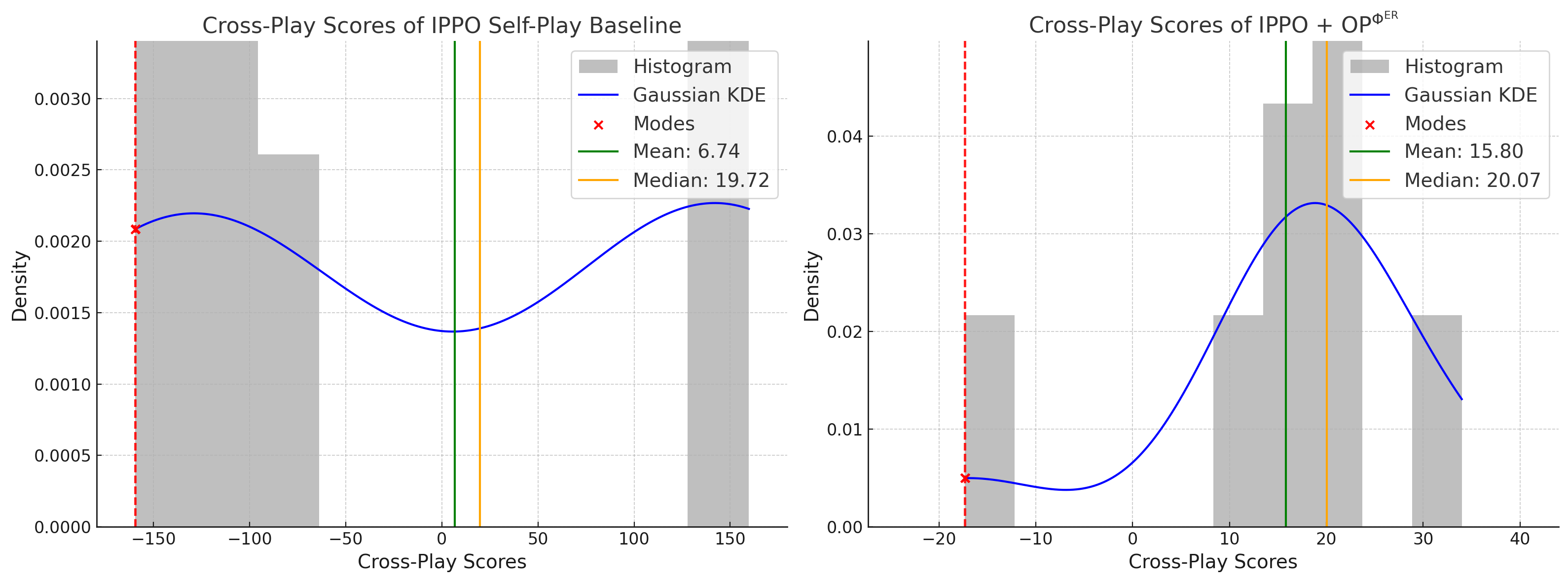
Figure 2: Cross-play score distribution of the IPPO self-play baseline population and the ER symmetry agent population in Overcooked V2. The baseline population achieves mean SP scores of $162.33\pm 0.14$, and the ER symmetry population achieves mean SP scores of $27.81\pm 0.3$.

The IPPO baseline population exhibits a highly bi-modal distribution of cross-play (XP) scores, where agents are either largely compatible or largely incompatible. In Figure 2, we plot the cross-play score distribution of both agent populations, and can see the SP-optimal IPPO baseline population achieves a mean cross-play score of $6.74$, whereas the $\text{OP}^{\Phi^{\text{ER}}}$-optimal population achieves a mean cross-play score of 15.8. In particular, the ER symmetry population is able to significantly close the self-play to cross-play (SP-XP) gap compared to the baseline population, demonstrating more consistent coordination across different agents. We emphasize that Overcooked V2 presents a challenging environment where agents move simultaneously, which renders standard methods like off-belief Learning (Hu et al., 2021) less applicable. This further highlights the effectiveness of ER symmetries in improving ZSC.

4.4 Hanabi

Hanabi (see Appendix F for details) is a challenging AI benchmark, and has served as the primary test bed for many algorithms designed for zero-shot coordination, ad-hoc teamplay, and other cooperative tasks (Bard et al., 2020; Cui et al., 2021; Nekoei et al., 2021; 2023; Muglich et al., 2022a; b).

Preserves OP Optimality

Since ER symmetries contain Dec-POMDP symmetries, and capture equivalences beyond just relabelling, they are clearly more diverse than Dec-POMDP symmetries, and hence better satisfy Item 1 from Section 3.1. We verify the ER symmetries also approximately satisfy Item 2.

We take the 11 learned regularized ER symmetries from above, denoting this set as $\hat{\Phi}^{\text{ER}}$. We find that $\mathbb{E}_{\pi\sim\Pi_{*}^{\hat{\Phi}^{\text{ER}}}}\left[\text{OP}^{\hat{\Phi}^{\text{ER}}}(\pi)\right]=23.59\pm 0.04$ and $\mathbb{E}_{\pi\sim\Pi_{*}^{\hat{\Phi}^{\text{ER}}}}\left[\mathbb{E}_{\phi\sim\hat{\Phi}^{\text{ER}}}\left[\text{OP}^{\hat{\Phi}^{\text{ER}}}(\phi(\pi))\right]\right]=23.34\pm 0.05$, where we train $5$ $\text{OP}^{\Phi^{\text{ER}}}$ policies. Thus, Item 2 is approximately satisfied by $\hat{\Phi}^{\text{ER}}$.

Zero-Shot Coordination

For ZSC, we train as baselines 1) a population of $5$ IPPO agents, and 2) a population of $5$ IPPO agents with access to all Dec-POMDP symmetries constrained by the OP objective in Equation 4. We train a population of ER symmetry agents that each independently discover ER symmetries for the OP objective. Each agent in the ER symmetry population uses $k=6$ seeds to learn ER symmetries, amongst which they save the $l=11$ that best preserve expected return. Each population (baseline and return symmetry populations alike) has a total of $5$ agents, where each agent trains $m=3$ policies and deploys the one achieving higher return.

Inspired by the symmetrizer in Treutlein et al. (2021); Muglich et al. (2022a); Van der Pol et al. (2020), we define the symmetrizer $S:\Pi\rightarrow\Pi$ by $S(\pi)(a_{t}\ |\ \tau_{t}):=\frac{1}{|[\pi]|}\sum_{\pi^{\prime}\in[\pi]}\pi^{\prime}(a_{t}\ |\ \tau_{t})$, where $\Phi$ can be taken to be either $\Phi^{\text{ER}}$ or $\Phi^{\text{MDP}}$. Agents from any population can thus transform their policy with $S$ before deploying for cross-play, ensuring invariance of the deployed policy w.r.t. $\Phi$ (since $\phi(S(\pi))=S(\pi),\forall\phi\in\Phi$). As per the empirical results below, the symmetrizer functions as a policy improvement operator for cross-play across multiple policy populations.

Table 1 shows that the agents using ER symmetries improve in ZSC over both baselines; this is even in spite of the Dec-POMDP agent population assuming access to environment symmetries. As well, even with just using a subset of transformations from $\Phi^{\text{ER}}$, the return symmetry agents are able to converge on policies that generalize well in cross-play. We also notice that symmetrization with respect to $\Phi^{\text{ER}}$ or $\Phi^{\text{MDP}}$ improves coordination amongst agents of all populations considered; we can see that $\Phi^{\text{ER}}$ better improves the optimal self-play policy population, and $\Phi^{\text{MDP}}$ better improves the other two, which aligns with expectation since $\Phi^{\text{ER}}$ is only explicitly enforced to maintain invariance over optimal self-play policies, whereas $\Phi^{\text{MDP}}$ maintains invariance over any policy type.

Table 1: Self-play, within-population mean cross-play (XP) and median cross-play (XP(*)) scores are reported. The $\text{OP}^{\Phi^{\text{MDP}}}$ population used all $120$ Dec-POMDP symmetries, whereas the $\text{OP}^{\Phi^{\text{ER}}}$ population used $11$ ER symmetries. “MDP” indicates the population was symmetrized with Dec-POMDP symmetries at test time, and “ER” analogously indicates symmetrization with expected return symmetries. The ER symmetrizer uses $11$ expected return symmetries.

Model	Self-Play	XP	XP(*)	XP(*)+MDP	XP(*)+ER
IPPO	$\mathbf{24.04\pm 0.02}$	$4.02\pm 0.17$	$0.12\pm 0.03$	$0.14\pm 0.03$	$0.10\pm 0.03$
IPPO + $\text{OP}^{\Phi^{\text{MDP}}}$	$23.81\pm 0.03$	$8.61\pm 0.17$	$8.14\pm 0.15$	$8.70\pm 0.16$	$9.91\pm 0.14$
IPPO + $\text{OP}^{\Phi^{\text{ER}}}$	$23.74\pm 0.03$	$\mathbf{21.64\pm 0.07}$	$\mathbf{22.03\pm 0.05}$	$\mathbf{22.50\pm 0.06}$	$\mathbf{22.25\pm 0.05}$

5 Related Work

Extensive research exists on coordination in multi-agent systems, particularly in zero-shot coordination. Methods like Hu et al. (2020); Muglich et al. (2022a) use Dec-POMDP symmetries to avoid incompatible policies, while Hu et al. (2021) rely on environment dynamics for grounded policies. Diversity-based approaches also leverage known symmetries and simulator access (Cui et al., 2023; Lupu et al., 2021). In contrast, ER symmetries can be learned from agent-environment interactions without privileged information, enabling grounded signaling and effective coordination in concurrent environments (see Sections 4.2 and 4.3).

In single-agent settings, symmetry has been shown to reduce sample complexity in RL (Van der Pol et al., 2020; Zhu et al., 2022; Nguyen et al., 2024). In multi-agent systems, symmetries reduce policy space complexity and help agents identify equivalent strategies (van der Pol et al., 2021; Muglich et al., 2022a). However, many methods require explicit knowledge of symmetries, or rely on predefined groups (Abreu et al., 2023; Yu et al., 2024; Nguyen et al., 2024). Our work generalizes these approaches by introducing ER symmetries, which do not require prior symmetry knowledge or equivariant networks, and can be learned directly through environment interactions.

Our work relates to value-based abstraction, which groups states or observations with similar value functions. Rezaei-Shoshtari et al. (2022) use lax-bisimulation to learn MDP homomorphisms, while Grimm et al. (2021) learn a model of the underlying MDP for value-based planning. In contrast, we focus on symmetries in the policy space that preserve expected return. ER symmetries are conceptually related to $Q^{*}$-irrelevance abstractions (Li et al., 2006) in that both aim to preserve the optimal value function of an MDP. However, whereas $Q^{*}$-irrelevance abstractions reduce complexity by aggregating states, ER symmetries form a group that acts bijectively on the policy space, transforming optimal policies into other policies with the same expected return.

6 Conclusion

This paper defined expected return symmetries—a group whose action preserves policy expected return. We demonstrated that the symmetries in this group can be learned purely from interactions with the environment and without requiring privileged environment information. We demonstrated that this symmetry class significantly enhances zero-shot coordination, significantly outperforming traditional Dec-POMDP symmetries, which are a subset of this group. Importantly, we showed that expected return symmetries are effective in challenging settings where state-of-the-art ZSC methods, such as off-belief learning (Hu et al., 2021) in Hanabi or approaches based on cognitive hierarchies, either fail completely (e.g., in the lever game and cat/dog environments) or face difficulties in their application (e.g., Overcooked V2).

One major limitation of our approach is that we constrain the search for symmetries to bijections over the action and observation spaces. While this works well in many settings, as shown in our experiments, there are environments, e.g. the two-lever game, in which this limited expressivity cannot provide enough diversity within the equivalence classes of policies that are optimal w.r.t. OP with $\Phi^{\text{ERS}}$, to prevent coordination failure in ZSC. Another limitation is that the success of our method is heavily dependent on the type of policies which are used to learn the ER symmetries.

Our work opens several avenues for future research. One direction is to explore the use of expected return symmetries in ad-hoc teamwork or single-agent settings. Another is to investigate broader classes of symmetries, beyond the ones that arise from bijections on the actions and observations.

Appendix A Experimental Setup

For expected return symmetry discovery in cat/dog, we use a temperature of $T=1/2.667$ for Boltzmann exploration to promote sufficient exploration of different actions. We use a constant baseline function with value $9.5$ for the policy gradient. We use a learning rate of $0.01$ and $2000$ episodes for each inner loop of Algorithm 1.

For expected return symmetry discovery in Overcooked V2 and Hanabi, we parameterize $\hat{\phi}_{\mathcal{O},\theta}$ as a two hidden layer, feedforward neural network, with each linear layer intialized as a $|\mathcal{O}^{i}|$-dimensional identity matrix; this choice of initialization is necessary as the symmetry discovery is highly initialization sensitive. We apply ReLU to the final output of the network to promote sparsity in the representation. We build on top of the environment implementation and baseline algorithms in JaxMARL (Rutherford et al., 2023).

For Hanabi, we run each inner loop of Algorithm 2 for $1.5\mathrm{e}{9}$ timesteps across vectorized Hanabi environments. As per Equation 3.3 we use $\lambda_{1}=0.65$, $\lambda_{2}=2.5\mathrm{e}{-9}$. $\phi_{\mathcal{A},\theta}$ is a fixed action transposition for each learned symmetry. We use a temperature of $T=1$ for Boltzmann exploration.

For Overcooked V2, we run each inner loop of Algorithm 3 for $1.5\mathrm{e}{8}$ timesteps. $\phi_{\mathcal{A},\theta}$ is a learned affine map. We use a temperature of $T=1.1$ for Boltzmann exploration.

For both Hanabi and Overcooked V2, we use PPO and Generalized Advantage Estimation. For Hanabi, we use $4$ epochs, $1024$ environments per pretrained policy, $128$ environment steps per update, $4$ minibatches, $\gamma=0.99$, GAE Lambda $=0.95$, CLIP EPS $=0.2$, VF COEFF = $0.5$, MAX GRAD NORM $=0.5$, a learning rate of $1\mathrm{e}{-5}$ and a linear learning rate annealing schedule. For Overcooked V2, we use $4$ epochs, $256$ environments, $256$ environment steps per update, $64$ minibatches, $\gamma=0.99$, GAE Lambda $=0.95$, CLIP EPS $=0.2$, VF COEFF $=0.5$, MAX GRAD NORM $=0.25$, a learning rate of $1\mathrm{e}{-5}$ with no annealing.

Methods for Hanabi and Overcooked V2 were ran on A40 and L40 GPUs.

Full working code for all four environments will be released soon.

Appendix B Proofs

Theorem.

$\Phi^{\text{ER}}:=\left\{\phi\in\Psi\ \middle|\forall\pi\in\Pi_{*}^{\epsilon}:\ J(\pi)=J(\phi(\pi))\right\}$ forms a group under function composition.

Proof.

To show that $\Phi^{\text{ER}}$ forms a group under function composition, we verify the group axioms: closure, associativity, identity, and inverses.

Closure: For any $\phi_{1},\phi_{2}\in\Phi^{\text{ER}}$, we need to show that $\phi_{1}\circ\phi_{2}\in\Phi^{\text{ER}}$. For the composition $\phi_{1}\circ\phi_{2}$, we need to check:

$$J(\pi)=J((\phi_{1}\circ\phi_{2})(\pi))$$

Since $\phi_{2}(\pi)\in\Phi^{\text{ER}}$ and $\phi_{1}(\pi^{\prime})\in\Phi^{\text{ER}}$ for all $\pi,\pi^{\prime}\in\Pi_{*}^{\epsilon}$:

$$J(\pi)=J(\phi_{2}(\pi))=J(\phi_{1}(\phi_{2}(\pi)))=J((\phi_{1}\circ\phi_{2})(\pi)).$$

Hence, $\phi_{1}\circ\phi_{2}\in\Phi^{\text{ER}}$, proving closure.

Associativity: Function composition is associative, so for any $\phi_{1},\phi_{2},\phi_{3}\in\Phi^{\text{ER}}$:

$$(\phi_{1}\circ\phi_{2})\circ\phi_{3}=\phi_{1}\circ(\phi_{2}\circ\phi_{3}).$$

Thus, associativity holds.

Identity: The identity function $\mathbf{Id}\in\Psi$ satisfies $\mathbf{Id}(\pi)=\pi$ for all $\pi\in\Pi$, and thus preserves the expected return of optimal policies $\pi\in\Pi_{*}^{\epsilon}$. Therefore, $\mathbf{Id}\in\Phi^{\text{ER}}$ and acts as the identity element.

Inverses: We let $\phi\in\Phi^{\text{ER}}$. Since $\Psi$ is a finite group, there exists a positive integer $k$ such that $\phi^{k}=\mathbf{Id}$, and thus $\phi^{-1}=\phi^{k-1}$. Since $\phi^{k-1}\in\Phi^{\text{ER}}$ due to closure, we see that $\phi^{-1}\in\Phi^{\text{ER}}$.

Since $\Phi^{\text{ER}}$ satisfies closure, associativity, identity, and inverses, it forms a group under function composition. ∎

Theorem.

For any Dec-POMDP symmetry $\phi\in\Phi^{\text{MDP}}$, and any joint policy $\pi$, it holds that $J(\pi)=J(\phi(\pi))$.

Proof.

Let $V_{\pi}(\tau_{t})$ denote the value of $\pi$ from $\tau_{t}$ onwards, i.e.

$$V_{\pi}(\tau_{t}):=\mathbb{E}_{\pi}\left[\sum_{t^{\prime}>t}^{H}\gamma^{t^{\prime}-t-1}r_{t^{\prime}}\Big{|}\tau_{t}\right]$$ (13)

We prove via induction over $t$, that $V_{\pi}(\tau_{t})=V_{\phi(\pi)}(\phi(\tau_{t}))$ for all AOHs $\tau_{t}$, for all $t=0,...,H$. Since this includes the empty starting AOH $\tau_{0}=\phi(\tau_{0})$, it follows that $J(\pi)=V_{\pi}(\tau_{0})=V_{\phi(\pi)}(\phi(\tau_{0}))=V_{\phi(\pi)}(\tau_{0})=J(\phi(\pi))$.

The base case for the induction is $V_{\pi}(\tau_{H})=0=V_{\phi(\pi)}(\phi(\tau_{H}))$, since at time $H$ the game ends. The induction hypothesis is that for a fixed $t$ it holds that $V_{\pi}(\tau_{t+1})=V_{\phi(\pi)}(\phi(\tau_{t+1}))$ for all AOHs $\tau_{t+1}$. For the induction step we use the Bellman equation:

$$V_{\pi}(\tau_{t})= \sum_{s_{t}\in\mathcal{S}}\mathcal{B}_{\pi}(s_{t}\ |\ \tau_{t})\sum_{a_{t}\in\mathcal{A}}\pi(a_{t}\ |\ \tau_{t})\sum_{s_{t+1}\in\mathcal{S}}\mathcal{T}(s_{t+1}\ |\ s_{t},a_{t})$$

$$\times\left[\mathcal{R}(s_{t+1},a_{t})+\gamma\sum_{o_{t+1}\in\mathcal{O}}\mathcal{U}(o_{t+1}\ |\ s_{t+1},a_{t})V_{\pi}(\tau_{t+1})\right],$$

where $\tau^{i}_{t+1}=(\tau^{i}_{t},a^{i}_{t},o^{i}_{t+1})$, and $\tau_{t+1}=(\tau^{1}_{t+1},\dots,\tau^{n}_{t+1})$. Thus we see that

$$V_{\phi(\pi)}(\phi(\tau_{t})) =\sum_{s_{t}\in\mathcal{S}}\mathcal{B}_{\phi(\pi)}(\phi(s_{t})\ |\ \phi(\tau_{t}))\sum_{a_{t}\in\mathcal{A}}\phi(\pi)(\phi(a_{t})\ |\ \phi(\tau_{t}))\sum_{s_{t+1}\in\mathcal{S}}\mathcal{T}(\phi(s_{t+1})\ |\ \phi(s_{t}),\phi(a_{t}))$$

$$\times\left[\mathcal{R}(\phi(s_{t}),\phi(a_{t}))\ +\gamma\sum_{o_{t+1}\in\mathcal{O}}\mathcal{U}(\phi(o_{t+1})\ |\ \phi(s_{t}),\phi(a_{t}))V_{\phi(\pi)}(\phi(\tau_{t+1}))\right]$$

$$= \sum_{s_{t}\in\mathcal{S}}\mathcal{B}_{\pi}(s_{t}\ |\ \tau_{t})\sum_{a_{t}\in\mathcal{A}}\pi(a_{t}\ |\ \tau_{t})\sum_{s_{t+1}\in\mathcal{S}}\mathcal{T}(s_{t+1}\ |\ s_{t},a_{t})$$

$$\times\Bigg{[}\mathcal{R}(s_{t+1},a_{t})+\gamma\sum_{o_{t+1}\in\mathcal{O}}\mathcal{U}(o_{t+1}\ |\ s_{t+1},a_{t})V_{\pi}(\tau_{t+1})\Bigg{]}$$

$$= V_{\pi}(\tau_{t}),$$

where the second equality follows from Equations 2 and 3, the fact that $B_{\phi(\pi)}(\phi(s_{t})|\phi(\tau_{t}))=B_{\pi}(s_{t}|\tau_{t})$ for all $s_{t}\in\mathcal{S}$ and AOHs $\tau_{t}$, and the induction hypothesis. This finishes the induction step, and thus the proof. ∎

Appendix C Learned Transformations Satisfy Group Properties

This section analyzes the learned ER symmetries for their group properties.

We first train six (near-)optimal IPPO policies with independent seeds as $\Pi^{\prime}$, obtaining a mean expected return of $\mathbb{E}_{\pi\sim\Pi^{\prime}}[J(\pi)]=24.04\pm 0.02$. Next, we randomly select $64$ action-space transpositions to fix as $\{\phi_{\mathcal{A},\theta_{l}}\}_{l=1}^{64}$, and learn the corresponding $\{\phi_{\mathcal{O},\theta_{l}}\}_{l=1}^{64}$ via optimizing Equation 10 / Algorithm 1. This is a significant undersampling of the 190 possible transpositions, yet as we show below we still learn effective ER symmetries for coordination. We then save the 11 best transformations (those that maximize Equation 10) as unregularized ER symmetries. These are used to maximize Equation 3.3 / Algorithm 2 on another set of $64$ random transpositions, now enforcing compositional closure and invertibility. The $8$ best are saved as regularized ER symmetries.

Table 2: Comparison of 11 unregularized and 11 regularized ER symmetries applied to 6 unseen optimal policies ($|\Pi_{\text{unseen}}|=6$). Regularization enforces compositionality and invertibility. For $k=1,2,3$, let $J_{k}=\mathbb{E}_{\phi_{i}\sim\Phi}\mathbb{E}_{\pi\sim\Pi_{\text{unseen}}}[J((\phi_{1}\circ\dots\circ\phi_{k})(\pi))]$ denote the expected return after composing $k$ randomly sampled transformations. We report Single Transform. ($J_{1}$), Double Comp. ($J_{2}$), and Triple Comp. ($J_{3}$). Relative Reconstruction Loss measures approximate invertibility (lower is better): $\mathbb{E}_{\pi\sim\Pi_{\text{unseen}}}\mathbb{E}_{\tau\sim\pi}[\frac{||\tau-\phi_{\mathcal{O}}^{2}(\tau)||}{||\tau||}]$, using the $\ell_{2}$ norm for AOH vectors. Recall $\mathbb{E}_{\pi\sim\Pi^{\prime}}[J(\pi)]=24.04\pm 0.02$.

	Single Transform.	Double Comp.	Triple Comp.	Rel. Rec. Loss
Unreg.	$22.88\pm 0.07$	$21.10\pm 0.09$	$20.36\pm 0.11$	$31.4\%\pm 1.8\%$
Reg.	$23.32\pm 0.05$	$22.16\pm 0.07$	$20.94\pm 0.12$	$16.7\%\pm 0.18\%$

Table 2 shows that up to minor deviations in expected return preservation, the learned ER symmetries still approximately satisfy closure under composition. In addition, when invertibility is enforced, the relative reconstruction loss decreases substantially (a lower relative reconstruction loss tells us applying the transformation twice brings us closer to the original AOH, suggesting approximate invertibility). We conclude that the learned ER symmetries, especially the regularized ones, approximately satisfy the desired group-theoretic properties.

Appendix D Algorithms

Algorithm 1 Learning Expected Return Symmetries with Policy Gradients (without enforcing compositionality nor invertibility) …Optimization of Equation 10

1:Input: A Dec-POMDP, a set $\Pi^{\prime}$ of joint policies in it, a parameterization $\phi_{\mathcal{O},\theta}$, $\theta\in\Theta$, a learning rate $\eta>0$, $l$ for the number of top transformations to save

2:Initialize list of top $l$ average expected returns: $\bar{J}_{\text{top}}=[-\infty,\dots,-\infty]$ (length $l$)

3:Initialize list of top $l$ transformations: $\phi_{\text{top}}=[\emptyset,\dots,\emptyset]$ (length $l$)

4:for each action transposition $\phi_{\mathcal{A}}\in\text{Transpositions}(\mathcal{A})$ do

5:  Initialize $\phi_{\mathcal{O},\theta}$ with random parameters $\theta\in\Theta$

6:  while not converged do

7:   for each policy $\pi\in\Pi^{\prime}$ do

8:     Sample a batch $\mathcal{B}$ of joint AOHs, and the corresponding sequences of returns, using the transformed policy $\phi_{\theta}(\pi)=(\phi_{\mathcal{A}},\phi_{\mathcal{O},\theta})(\pi)$

9:     Compute advantage $A^{\phi_{\theta}(\pi)}(\tau_{t},a_{t})$ for all $t=0,...,H-1$, using any advantage function (e.g., TD, GAE)

10:     Compute policy gradient:

$$\nabla_{\theta}J(\phi_{\theta}(\pi))\approx\frac{1}{|\mathcal{B}|}\sum_{\tau_{H}\in\mathcal{B}}\left[\sum_{t=0}^{H-1}\nabla_{\theta}\log\phi_{\theta}(\pi)(a_{t}\ |\ \tau_{t})A^{\phi_{\theta}(\pi)}(\tau_{t},a_{t})\right]$$

11:     Update parameters: $\theta\leftarrow\theta+\eta\nabla_{\theta}J(\phi_{\theta}(\pi))$

12:   end for

13:  end while

14:  Compute average expected return $\bar{J}_{\phi_{\theta}}$, where for every $\pi\in\Pi^{\prime}$ the expected return $J(\phi_{\theta}(\pi))$ is approximated by the average return over a number of episodes:

$$\bar{J}_{\phi_{\theta}}\approx\frac{1}{|\Pi^{\prime}|}\sum_{\pi\in\Pi^{\prime}}J(\phi_{\theta}(\pi))$$

15:  Find the index of the lowest return in $\bar{J}_{\text{top}}$, say $i_{\text{min}}$

16:  if $\bar{J}_{\phi_{\theta}}>\bar{J}_{\text{top}}[i_{\text{min}}]$ then

17:   Replace the lowest return: $\bar{J}_{\text{top}}[i_{\text{min}}]\leftarrow\bar{J}_{\phi_{\theta}}$

18:   Replace the corresponding transformation: $\phi_{\text{top}}[i_{\text{min}}]\leftarrow(\phi_{\mathcal{O},\theta},\phi_{\mathcal{A},\theta})$:

19:  end if

20:end for

21:Output: Set $\phi_{\text{top}}$ of the best $l$ learned transformations

Algorithm 2 Learning Expected Return Symmetries (enforcing compositionality and invertibility) …Optimization of Equation 3.3

1:Input: A Dec-POMDP, a set $\Pi^{\prime}$ of joint policies in it, a parameterization $\phi_{\mathcal{O},\theta}$, $\theta\in\Theta$, a learning rate $\eta>0$, transformations $\{\phi_{1},\dots,\phi_{m}\}$ obtained from Algorithm 1, $l$ for the number of top transformations to save, regularization weights $\lambda_{1},\lambda_{2}$

2:Initialize list of top $l$ average expected returns: $\bar{J}_{\text{top}}=[-\infty,\dots,-\infty]$ (length $l$)

3:Initialize list of top $l$ transformations: $\phi_{\text{top}}=[\emptyset,\dots,\emptyset]$ (length $l$)

4:for each transposition $\phi_{\mathcal{A}}\in\text{Transpositions}(\mathcal{A})$ do

5:  Initialize $\phi_{\mathcal{O},\theta}$ with random $\theta\in\Theta$

6:  while not converged do

7:   for each policy $\pi\in\Pi^{\prime}$ do

8:     With probability $1-\lambda_{1}$ set $\tilde{\phi}_{\theta}=\phi_{\theta}$, and with probability $\lambda_{1}$ sample $\phi_{i},\phi_{j}\in\{\phi_{1},\dots,\phi_{m}\}$ and set $\tilde{\phi}_{\theta}=\phi_{i}\circ\phi_{\theta}\circ\phi_{j}$

9:     Sample a batch $\mathcal{B}$ of joint AOHs, and the corresponding sequences of returns, using the transformed policy $\tilde{\phi}_{\theta}(\pi)$

10:     Compute advantage $A^{\tilde{\phi}_{\theta}(\pi)}(\tau_{t},a_{t})$, for all $t=0,...,H-1$, using any advantage function (e.g., TD, GAE)

11:     Compute the invertibility regularization term $L(\theta)=\frac{1}{|\mathcal{O}|}\sum_{o\in\mathcal{O}}\left[d(o,\phi_{\mathcal{O},\theta}^{2}(o))^{2}\right]$, and its gradient $\nabla_{\theta}L(\theta)$

12:     Compute policy gradient:

$$\nabla_{\theta}J(\tilde{\phi}_{\theta}(\pi))\approx\frac{1}{|\mathcal{B}|}\sum_{\tau_{H}\in\mathcal{B}}\left[\sum_{t=0}^{H-1}\nabla_{\theta}\log\tilde{\phi}_{\theta}(\pi)(a_{t}\mid\tau_{t})A^{\tilde{\phi}_{\theta}(\pi)}(\tau_{t},a_{t})\right]$$

13:     Update $\theta\leftarrow\theta+\eta\big{(}\nabla_{\theta}J(\tilde{\phi}_{\theta}(\pi))-\lambda_{2}\nabla_{\theta}L(\theta)\big{)}$

14:   end for

15:   Compute average expected return $\bar{J}_{\phi_{\theta}}$, where for every $\pi\in\Pi^{\prime}$ the expected return $J(\phi_{\theta}(\pi))$ is approximated by the average return over a number of episodes

$$\bar{J}_{\phi_{\theta}}\approx\frac{1}{|\Pi^{\prime}|}\sum_{\pi\in\Pi^{\prime}}J(\phi_{\theta}(\pi))$$

16:  end while

17:  Find the index of the lowest return in $\bar{J}_{\text{top}}$, say $i_{\text{min}}$

18:  if $\bar{J}_{\phi_{\theta}}>\bar{J}_{\text{top}}[i_{\text{min}}]$ then

19:   Replace the lowest return: $\bar{J}_{\text{top}}[i_{\text{min}}]\leftarrow\bar{J}_{\phi_{\theta}}$

20:   Replace the corresponding transformation: $\phi_{\text{top}}[i_{\text{min}}]\leftarrow(\phi_{\mathcal{O},\theta},\phi_{\mathcal{A},\theta})$

21:  end if

22:end for

23:Output: Set $\phi_{\text{top}}$ of the best $l$ learned transformations

Algorithm 3 Learning Expected Return Symmetries through cross-play maximization between pairs of Policies …Optimization of Equation 12

1:Input: A Dec-POMDP, a set $\Pi^{\prime}$ of joint policies in it, a parameterization $\phi_{\mathcal{O},\theta}$, $\theta\in\Theta$, a learning rate $\eta>0$, $l$ for the number of top transformations to save

2:Initialize list of top $l$ average expected returns: $\bar{J}_{\text{top}}=[-\infty,\dots,-\infty]$ (length $l$)

3:Initialize list of top $l$ transformations: $\phi_{\text{top}}=[\emptyset,\dots,\emptyset]$ (length $l$)

4:for each pair of joint policies $(\pi_{i},\pi_{j})\in\Pi^{\prime}\times\Pi^{\prime}\setminus\{(\pi,\pi)\,|\,\pi\in\Pi^{\prime}\}$ do

5:  Initialize $\phi_{\mathcal{O},\theta}$ and $\phi_{\mathcal{A},\theta}$ with random parameters $\theta\in\Theta$

6:  while not converged do

7:   Sample a batch $\mathcal{B}$ of joint AOHs, and the corresponding sequences of returns, using the transformed pair $(\pi_{i}^{1},\phi_{\theta}(\pi_{j}^{2}))$

8:   Compute advantage $A^{(\pi_{i}^{1},\phi_{\theta}(\pi_{j}^{2}))}(\tau_{t},a_{t})$, for all $t=0,...,H-1$, using any advantage function (e.g., TD, GAE)

9:   Compute policy gradient:

$$\nabla_{\theta}J(\pi_{i}^{1},\phi_{\theta}(\pi_{j}^{2}))\approx\frac{1}{|\mathcal{B}|}\sum_{\tau_{H}\in\mathcal{B}}\left[\sum_{t=0}^{H-1}\nabla_{\theta}\log\phi_{\theta}(\pi_{j}^{2})(a_{t}\ |\ \tau_{t})A^{(\pi_{i}^{1},\phi_{\theta}(\pi_{j}^{2}))}(\tau_{t},a_{t})\right]$$

10:   Update parameters: $\theta\leftarrow\theta+\eta\nabla_{\theta}J(\pi_{i}^{1},\phi_{\theta}(\pi_{j}^{2}))$

11:   Compute average return $\bar{J}_{(\pi_{i}^{1},\phi_{\theta}(\pi_{j}^{2}))}\approx J(\pi_{i}^{1},\phi_{\theta}(\pi_{j}^{2}))$ over a number of episodes

12:  end while

13:  Find the index of the lowest return in $\bar{J}_{\text{top}}$, say $i_{\text{min}}$

14:  if $\bar{J}_{(\pi_{i}^{1},\phi_{\theta}(\pi_{j}^{2}))}>\bar{J}_{\text{top}}[i_{\text{min}}]$ then

15:   Replace the lowest return: $\bar{J}_{\text{top}}[i_{\text{min}}]\leftarrow\bar{J}_{(\pi_{i}^{1},\phi_{\theta}(\pi_{j}^{2}))}$

16:   Replace the corresponding transformation: $\phi_{\text{top}}[i_{\text{min}}]\leftarrow(\phi_{\mathcal{O},\theta},\phi_{\mathcal{A},\theta})$

17:  end if

18:end for

19:Output: Set $\phi_{\text{top}}$ of the best $l$ learned transformations

Appendix E Interpretability of Hanabi OP Agents

Figure 3: Conditional action matrices of $\text{OP}^{\Phi^{\text{MDP}}}$-optimal and $\text{OP}^{\Phi^{\text{ER}}}$-optimal policies; i.e., $P(a_{t}^{i}\ |\ a_{t-1}^{j})$. We select the agent from both respective populations achieving the highest cross-play scores. We can see the $\text{OP}^{\Phi^{\text{ER}}}$-optimal policy more consistently uses a rank hint to signal playing the fifth card, whereas the $\text{OP}^{\Phi^{\text{MDP}}}$-optimal policy uses a similar convention but less consistently.

Appendix F Hanabi

Hanabi is a cooperative card game that can be played with 2 to 5 people. Hanabi is a popular game, having been crowned the 2013 “Spiel des Jahres” award, a German industry award given to the best board game of the year. Hanabi has been proposed as an AI benchmark task to test models of cooperative play that act under partial information Bard et al. (2020). To date, Hanabi has one of the largest state spaces of all Dec-POMDP benchmarks.

The deck of cards in Hanabi is comprised of five colors (white, yellow, green, blue and red), and five ranks (1 through 5), where for each color there are three 1’s, two each of 2’s, 3’s and 4’s, and one 5, for a total deck size of fifty cards. Each player is dealt five cards (or four cards if there are 4 or 5 players). At the start, the players collectively have eight information tokens and three fuse tokens, the uses of which shall be explained presently.

In Hanabi, players can see all other players’ hands but their own. The goal of the game is to play cards to collectively form five consecutively ordered stacks, one for each color, beginning with a card of rank 1 and ending with a card of rank 5. These stacks are referred to as fireworks, as playing the cards in order is meant to draw analogy to setting up a firework display.

We call the player whose turn it is the active agent. The active agent must conduct one of three actions:

• Hint - The active agent chooses another player to grant a hint to. A hint involves the active agent choosing a color or rank, and revealing to their chosen partner all cards in the partner’s hand that satisfy the chosen color or rank. Performing a hint exhausts an information token. If the players have no information tokens, a hint may not be conducted and the active agent must either conduct a discard or a play.

• Discard - The active agent chooses one of the cards in their hand to discard. The identity of the discarded card is revealed to the active agent and becomes public information. Discarding a card replenishes an information token should the players have less than eight.

• Play - The active agent attempts to play one of the cards in their hand. The identity of the played card is revealed to the active agent and becomes public information. The active agent has played successfully if their played card is the next in the firework of its color to be played, and the played card is then added to the sequence. If a firework is completed, the players receive a new information token should they have less than eight. If the player is unsuccessful, the card is discarded, without replenishment of an information token, and the players lose a fuse token.

The game ends when all three fuse tokens are spent, when the players successfully complete all five fireworks, or when the last card in the deck is drawn and all players take one last turn. If the game finishes by depletion of all fuse tokens (i.e. by “bombing out”), the players receive a score of 0. Otherwise, the score of the finished game is the sum of the highest card ranks in each firework, for a highest possible score of 25.

More facts about Hanabi:

1. The Dec-POMDP symmetries correspond to permutations of the five card colors ($5!=120$).

2. In two-player Hanabi, there are $20$ possible actions per turn, organized into four types: Play, Discard, Color Hint, and Rank Hint. These yield $190$ distinct action transpositions.

3. A perfect score is $25$, though some deck permutations make this score unreachable, so no policy can guarantee an expected return of $25$.

References

- Abreu et al. (2023) Miguel Abreu, Luis Paulo Reis, and Nuno Lau. Addressing Imperfect Symmetry: a Novel Symmetry-Learning Actor-Critic Extension. arXiv preprint arXiv:2309.02711, 2023.
- Bard et al. (2020) Nolan Bard, Jakob N Foerster, Sarath Chandar, Neil Burch, Marc Lanctot, H Francis Song, Emilio Parisotto, Vincent Dumoulin, Subhodeep Moitra, Edward Hughes, et al. The Hanabi Challenge: A New Frontier for AI Research. Artificial Intelligence, 280:103216, 2020.
- Bronstein et al. (2021) Michael M Bronstein, Joan Bruna, Taco Cohen, and Petar Veličković. Geometric Deep Learning: Grids, Groups, Graphs, Geodesics, and Gauges. arXiv preprint arXiv:2104.13478, 2021.
- Camerer et al. (2004) Colin F Camerer, Teck-Hua Ho, and Juin-Kuan Chong. A Cognitive Hierarchy Model of Games. The Quarterly Journal of Economics, 119(3):861–898, 2004.
- Carroll et al. (2019) Micah Carroll, Rohin Shah, Mark K Ho, Tom Griffiths, Sanjit Seshia, Pieter Abbeel, and Anca Dragan. On the Utility of Learning about Humans for Human-AI Coordination. Advances in Neural Information Processing Systems, 32, 2019.
- Chess.com (2021) Chess.com. The Worst And The Best Chess Handshakes Of World Cup 2021. https://www.youtube.com/watch?v=6fS7bDyNYHI, 2021. Accessed: 2024-09-30.
- Cohen et al. (2019) Taco Cohen, Maurice Weiler, Berkay Kicanaoglu, and Max Welling. Gauge Equivariant Convolutional Networks and the Icosahedral CNN. In International Conference on Machine learning, pp. 1321–1330. PMLR, 2019.
- Cui et al. (2021) Brandon Cui, Hengyuan Hu, Luis Pineda, and Jakob Foerster. K-level Reasoning for Zero-Shot Coordination in Hanabi. Advances in Neural Information Processing Systems, 34:8215–8228, 2021.
- Cui et al. (2023) Brandon Cui, Andrei Lupu, Samuel Sokota, Hengyuan Hu, David J Wu, and Jakob Foerster. Adversarial Diversity in Hanabi. In International Conference on Learning Representations, 2023.
- Finzi et al. (2020) Marc Finzi, Samuel Stanton, Pavel Izmailov, and Andrew Gordon Wilson. Generalizing Convolutional Neural Networks for Equivariance to Lie Groups on Arbitrary Continuous Data. In International Conference on Machine Learning, pp. 3165–3176. PMLR, 2020.
- Gessler et al. (2025) Tobias Gessler, Tin Dizdarevic, Ani Calinescu, Benjamin Ellis, Andrei Lupu, and Jakob Foerster. OvercookedV2: Rethinking Overcooked for Zero-Shot Coordination. In International Conference on Learning Representations, 2025.
- Grimm et al. (2021) Christopher Grimm, André Barreto, Greg Farquhar, David Silver, and Satinder Singh. Proper Value Equivalence. Advances in Neural Information Processing Systems, 34:7773–7786, 2021.
- Hu et al. (2020) Hengyuan Hu, Adam Lerer, Alex Peysakhovich, and Jakob Foerster. ”Other-Play” for Zero-Shot Coordination. In International Conference on Machine Learning, pp. 4399–4410. PMLR, 2020.
- Hu et al. (2021) Hengyuan Hu, Adam Lerer, Brandon Cui, Luis Pineda, Noam Brown, and Jakob Foerster. Off-Belief Learning. In International Conference on Machine Learning, pp. 4369–4379. PMLR, 2021.
- Ji et al. (2023) Jiaming Ji, Tianyi Qiu, Boyuan Chen, Borong Zhang, Hantao Lou, Kaile Wang, Yawen Duan, Zhonghao He, Jiayi Zhou, Zhaowei Zhang, et al. AI Alignment: A Comprehensive Survey. arXiv preprint arXiv:2310.19852, 2023.
- Kakish et al. (2019) Zahi M Kakish, F RodrÃguez-Lera, D Bischel, A Mosquera, R Boumghar, S Kaczmarek, T Seabrook, P Metzger, and JL Galanche. Open-source AI Assistant for Cooperative Multi-agent Systems for Lunar Prospecting Missions. In 8th European Conference for Aeronautics and Space Sciences (EUCASS), 2019.
- Krizhevsky et al. (2017) Alex Krizhevsky, Ilya Sutskever, and Geoffrey E Hinton. ImageNet Classification with Deep Convolutional Neural Networks. Communications of the ACM, 60(6):84–90, 2017.
- Li et al. (2006) Lihong Li, Thomas J Walsh, and Michael L Littman. Towards a Unified Theory of State Abstraction for MDPs. AI&M, 1(2):3, 2006.
- Lupu et al. (2021) Andrei Lupu, Brandon Cui, Hengyuan Hu, and Jakob Foerster. Trajectory Diversity for Zero-Shot Coordination. In International Conference on Machine Learning, pp. 7204–7213. PMLR, 2021.
- Mariani et al. (2021) Stefano Mariani, Giacomo Cabri, and Franco Zambonelli. Coordination of Autonomous Vehicles: Taxonomy and Survey. ACM Computing Surveys (CSUR), 54(1):1–33, 2021.
- Muglich et al. (2022a) Darius Muglich, Christian Schroeder de Witt, Elise van der Pol, Shimon Whiteson, and Jakob Foerster. Equivariant Networks for Zero-Shot Coordination. Advances in Neural Information Processing Systems, 35:6410–6423, 2022a.
- Muglich et al. (2022b) Darius Muglich, Luisa M Zintgraf, Christian A Schroeder De Witt, Shimon Whiteson, and Jakob Foerster. Generalized Beliefs for Cooperative AI. In International Conference on Machine Learning, pp. 16062–16082. PMLR, 2022b.
- Narayanamurthy & Ravindran (2008) Shravan Matthur Narayanamurthy and Balaraman Ravindran. On the hardness of finding symmetries in Markov decision processes. In International Conference on Machine learning, pp. 688–695, 2008.
- Nekoei et al. (2021) Hadi Nekoei, Akilesh Badrinaaraayanan, Aaron Courville, and Sarath Chandar. Continuous Coordination As a Realistic Scenario for Lifelong Learning. In International Conference on Machine Learning, pp. 8016–8024. PMLR, 2021.
- Nekoei et al. (2023) Hadi Nekoei, Xutong Zhao, Janarthanan Rajendran, Miao Liu, and Sarath Chandar. Towards Few-shot Coordination: Revisiting Ad-hoc Teamplay Challenge In the Game of Hanabi. In Conference on Lifelong Learning Agents, pp. 861–877. PMLR, 2023.
- Nguyen et al. (2024) Hai Nguyen, Tadashi Kozuno, Cristian C Beltran-Hernandez, and Masashi Hamaya. Symmetry-aware Reinforcement Learning for Robotic Assembly under Partial Observability with a Soft Wrist. arXiv preprint arXiv:2402.18002, 2024.
- Oliehoek et al. (2007) Frans A Oliehoek, Matthijs TJ Spaan, Nikos Vlassis, et al. Dec-POMDPs with delayed communication. In The 2nd Workshop on Multi-agent Sequential Decision-Making in Uncertain Domains. Citeseer, 2007.
- Resnick et al. (2018) Cinjon Resnick, Ilya Kulikov, Kyunghyun Cho, and Jason Weston. Vehicle Communication Strategies for Simulated Highway Driving. arXiv preprint arXiv:1804.07178, 2018.
- Rezaei-Shoshtari et al. (2022) Sahand Rezaei-Shoshtari, Rosie Zhao, Prakash Panangaden, David Meger, and Doina Precup. Continuous MDP Homomorphisms and Homomorphic Policy Gradient. Advances in Neural Information Processing Systems, 35:20189–20204, 2022.
- Rutherford et al. (2023) Alexander Rutherford, Benjamin Ellis, Matteo Gallici, Jonathan Cook, Andrei Lupu, Gardar Ingvarsson, Timon Willi, Akbir Khan, Christian Schroeder de Witt, Alexandra Souly, Saptarashmi Bandyopadhyay, Mikayel Samvelyan, Minqi Jiang, Robert Tjarko Lange, Shimon Whiteson, Bruno Lacerda, Nick Hawes, Tim Rocktaschel, Chris Lu, and Jakob Nicolaus Foerster. JaxMARL: Multi-Agent RL Environments and Algorithms in JAX. arXiv preprint arXiv:2311.10090, 2023.
- Samuel (1959) Arthur L Samuel. Some Studies in Machine Learning Using the Game of Checkers. IBM Journal of research and development, 3(3):210–229, 1959.
- Sutton et al. (1999) Richard S Sutton, David McAllester, Satinder Singh, and Yishay Mansour. Policy Gradient Methods for Reinforcement Learning with Function Approximation. Advances in Neural Information Processing Systems, 12, 1999.
- Tan (1993) Ming Tan. Multi-Agent Reinforcement Learning: Independent vs. Cooperative Agents. In International Conference on Machine Mearning, pp. 330–337, 1993.
- Tesauro et al. (1995) Gerald Tesauro et al. Temporal difference learning and TD-Gammon. Communications of the ACM, 38(3):58–68, 1995.
- Treutlein et al. (2021) Johannes Treutlein, Michael Dennis, Caspar Oesterheld, and Jakob Foerster. A New Formalism, Method and Open Issues for Zero-Shot Coordination. In International Conference on Machine Learning, pp. 10413–10423. PMLR, 2021.
- Van der Pol et al. (2020) Elise Van der Pol, Daniel Worrall, Herke van Hoof, Frans Oliehoek, and Max Welling. MDP Homomorphic Networks: Group Symmetries in Reinforcement Learning. Advances in Neural Information Processing Systems, 33:4199–4210, 2020.
- van der Pol et al. (2021) Elise van der Pol, Herke van Hoof, Frans A Oliehoek, and Max Welling. Multi-Agent MDP Homomorphic Networks. In International Conference on Learning Representations, 2021.
- Yu et al. (2022) Chao Yu, Akash Velu, Eugene Vinitsky, Jiaxuan Gao, Yu Wang, Alexandre Bayen, and Yi Wu. The Surprising Effectiveness of PPO in Cooperative, Multi-Agent Games. Advances in Neural Information Processing Systems, 35:24611–24624, 2022.
- Yu et al. (2024) Xin Yu, Rongye Shi, Pu Feng, Yongkai Tian, Simin Li, Shuhao Liao, and Wenjun Wu. Leveraging Partial Symmetry for Multi-Agent Reinforcement Learning. In Proceedings of the AAAI Conference on Artificial Intelligence, volume 38, pp. 17583–17590, 2024.
- Zhu et al. (2022) Xupeng Zhu, Dian Wang, Ondrej Biza, Guanang Su, Robin Walters, and Robert Platt. Sample Efficient Grasp Learning Using Equivariant Models. arXiv preprint arXiv:2202.09468, 2022.