PUATE: Semiparametric Efficient Average Treatment Effect Estimation from Treated (Positive) and Unlabeled Units

Abstract

The estimation of average treatment effects (ATEs), defined as the difference in expected outcomes between treatment and control groups, is a central topic in causal inference. This study develops semiparametric efficient estimators for ATE estimation in a setting where only a treatment group and an unknown group—comprising units for which it is unclear whether they received the treatment or control—are observable. This scenario represents a variant of learning from positive and unlabeled data (PU learning) and can be regarded as a special case of ATE estimation with missing data. For this setting, we derive semiparametric efficiency bounds, which provide lower bounds on the asymptotic variance of regular estimators. We then propose semiparametric efficient ATE estimators whose asymptotic variance aligns with these efficiency bounds. Our findings contribute to causal inference with missing data and weakly supervised learning.

1 Introduction

The estimation of average treatment effects (ATEs), defined as the difference in expected outcomes between treatment and control groups, is a fundamental problem in causal inference (Imbens & Rubin, 2015). Estimating ATEs allows researchers to quantify the causal impact of a treatment, intervention, or policy on an outcome of interest. This problem is of paramount importance across various fields, including economics, healthcare, and social sciences.

Standard ATE estimation typically assumes access to both treatment and control groups with complete treatment assignment information. However, in many practical cases, this assumption does not hold, and there may only be a treatment group and an unknown group, where the treatment assignment is not observable. Such scenarios arise in applications, including recommendation systems with implicit feedback, electronic health records, and marketing campaigns, where the absence of explicit treatment information presents significant challenges for causal inference.

For example, in recommendation systems, if a user buys a product from a website, we can determine that the user visited the website. However, if the user buys a product in an in-person shop, we cannot know whether the user visited the website. If creating an online website is considered a treatment, this scenario implies that users who bought the product at the shop belong to an unknown group.

1.1 Content of this study

We address the problem of ATE estimation only using a treatment group and an unknown group. This setting is closely related to learning from positive and unlabeled data (PU learning, Sugiyama et al., 2022), where the goal is to train a classifier using only positive and unlabeled data. In our context, the challenge lies in leveraging the treatment (positive) and unknown groups to estimate ATEs efficiently. We refer to our setting and methodology as PUATE.

For this problem, we first derive semiparametric efficiency bounds, which are the theoretical lower bounds on the asymptotic variance of regular estimators under the given data-generating processes (DGPs). These bounds serve as benchmarks for evaluating estimator performance. In this process, we compute the efficient influence function, which offers insights into constructing efficient estimators.

Then, using the efficient influence function, we develop semiparametric efficient ATE estimators that are $\sqrt{n}$-consistent and whose asymptotic variance achieves the efficiency bounds. These estimators thus attain optimality under the semiparametric framework.

In this study, we introduce two DGPs relevant to the PU setup: the censoring setting and the case-control setting (Elkan & Noto, 2008). In the censoring setting, we are provided with a single dataset in which some units have missing treatment information while others are confirmed to have received treatment. In the case-control setting, we are given two datasets: one containing treated units and the other containing units with unknown treatment status.

Specifically, our contributions are as follows:

• We formulate the ATE estimation problem with missing data using the frameworks of PU learning.

• We derive efficiency bounds in these settings.

• We propose novel efficient estimators.

• We establish connections between ATE estimation with missing data and PU learning.

• We also propose other candidates for estimators.

This study is organized as follows. We review related work in Section 1.2 and Appendix A. Section 2 formulates our problem. Section 3 discusses the identification of the ATE. In Section 4, we derive the efficiency bounds, propose an efficient estimator, and show the asymptotic properties for the censoring setting. Section 5 develops them for the case-control setting. Section 6 demonstrates simulation studies.

1.2 Related work

Our study is related to ATE estimation with missing values. There are various settings regarding how data is missing. For example, there are studies considering missing covariates (Zhao & Ding, 2024). This study focuses on the case with fully observed covariates and missing treatments.

Missing treatment information is common in observational studies (Kennedy, 2020). Molinari (2010) presents various examples in survey analysis. Ahn et al. (2011) examines the effect of physical activity on colorectal cancer using data with missing treatment for about $20$% of the units. Zhang et al. (2013) estimates the infant weight where the treatment, mother’s body mass index (BMI), is missing for about half of the units. Kuzmanovic et al. (2023) develops a conditional ATE estimation method in this setting.

Our formulation is inspired by PU learning in weakly supervised learning. PU learning studies can be traced back to case-control studies with contaminated controls (Steinberg & Cardell, 1992; Lancaster & Imbens, 1996). This setting is refined in du Plessis et al. (2015) as case-control PU learning. Elkan & Noto (2008) explores PU learning, particularly in the censoring setting. PU learning also has a connection to density-ratio estimation (Sugiyama et al., 2012; Qin, 1998; Kato & Teshima, 2021).

2 Problem setting

2.1 Potential outcomes

We consider two treatments, $1$ and $0$. For each treatment $d\in\{1,0\}$, there exists a potential outcome $Y(d)\in{\mathbb{R}}$. The outcome is observed only when the corresponding treatment is assigned to a unit. Each unit has $p$-dimensional covariates $X\in{\mathcal{X}}\subset{\mathbb{R}}^{p}$. This setting is called the Neyman-Rubin causal model (Neyman, 1923; Rubin, 1974).

Let $P_{0}$ denote the distribution of $Y(d)$ and $X$, along with other random variables introduced below. For simplicity, we assume that $P_{0}$ has a density. We denote the conditional density of $Y(d)$ given $X$ by $p_{Y(d),0}(y(d)\mid X)$, and the marginal density of $X$ by $\zeta_{0}(x)$.

We consider $n$ units, each of which receives either treatment or control. Let $Y_{i}(d)$ and $X_{i}$ be i.i.d. copies of $Y(d)$ and $X$. Throughout this study, for a random variable $R$, let $R_{i}$ be its i.i.d. copy under $P_{0}$. If unit $i$ receives treatment $d$, we observe $Y_{i}(d)$ but not the counterfactual outcome.

We refer to the group of units who receive treatment $1$ as the treatment group and those who receive treatment $0$ as the control group. In our setting, as formulated in the next subsection, we consider a scenario where part of the treatment group and a mixture of the treatment and control groups are observable, where the treatment indicator is unobservable. We refer to this mixed group as the unknown group.

2.2 Parameter of interest

Our objective is to estimate the ATE under $P_{0}$ using observed data, defined as

$$\tau_{0}\coloneqq{\mathbb{E}}\left[Y(1)-Y(0)\right],$$

where ${\mathbb{E}}$ denotes the expectation under $P_{0}$.

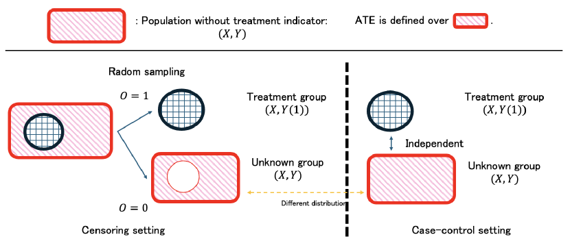
Figure 1: Illustration of the censoring and case-control settings

2.3 Observations

In our setting, the observations are non-standard. We can only observe part of the treatment group and the unknown group, a mixture of the treatment and control groups. This setting is a variant of PU learning.

PU learning encompasses two settings: the censoring setting and the case-control setting. In the censoring setting, we consider a single dataset with i.i.d. observations, where treatment labels contain missing values. Specifically, while part of the treatment group is observed, the mixture of the treated and control groups is also present. In the case-control setting, we observe two independent datasets: one consisting solely of the treatment group and the other comprising the unknown group. The censoring and case-control settings are also referred to as one-sample and two-sample settings, respectively (Niu et al., 2016). The case-control setting can also be regarded as a form of stratified sampling.

Censoring setting. In the censoring setting, we observe a single dataset ${\mathcal{D}}$, defined as follows:

$${\mathcal{D}}\coloneqq\left\{\big{(}X_{i},O_{i},Y_{i}\big{)}\right\}^{n}_{i=1},\ \ \big{(}X_{i},O_{i},Y_{i}\big{)}\sim p_{0}(x,o,y),$$

where $O_{i}\in\{1,0\}$ is an observation indicator with the observation probability $\pi_{0}(O\mid X)$, $Y_{i}$ is defined as

$$Y_{i} =\mathbbm{1}[O_{i}=1]Y_{i}(1)+\mathbbm{1}[O_{i}=0]Z_{i},$$

$$Z_{i} =\mathbbm{1}[\widetilde{D}_{i}=1]Y_{i}(1)+\mathbbm{1}[\widetilde{D}_{i}=0]Y_{i}(0),$$

and $\widetilde{D}_{i}\in\{1,0\}$ is a (latent) treatment indicator whose conditional probability given $O_{i}=0$ is $g_{0}(\widetilde{D}\mid X)={\mathbb{P}}(\widetilde{D}\mid X,O=0)$. We also refer to $g_{0}(d\mid X)$ as the propensity score. Here, the density $p_{0}(x,o,y)$ is defined as

$$p_{0}(x,o,y)=\zeta_{0}(x)\pi_{0}(o\mid x)p_{Y,0}(y\mid X=x),$$

where $p_{Y,0}$ is the density of $Y_{i}$.

Case-control setting. In the case-control setting, we observe two stratified datasets, ${\mathcal{D}}_{{\mathrm{T}}}$ and ${\mathcal{D}}_{{\mathrm{U}}}$, defined as

$${\mathcal{D}}_{{\mathrm{T}}}\coloneqq\left\{\big{(}X_{{\mathrm{T}},j},Y_{j}(1)\big{)}\right\}^{m}_{j=1},\,\big{(}X_{{\mathrm{T}},j},Y_{j}(1)\big{)}\sim p_{{\mathrm{T}},0}(x,y(1)),$$

$${\mathcal{D}}_{{\mathrm{U}}}\coloneqq\left\{\big{(}X_{k},Y_{{\mathrm{U}},k}\big{)}\right\}^{l}_{k=1},\ \big{(}X_{k},Y_{{\mathrm{U}},k}\big{)}\sim p_{{\mathrm{U}},0}(x,y_{{\mathrm{U}}}),$$

where $m$ and $l$ are fixed sample sizes of each dataset such that $m+l=n$, $X_{{\mathrm{T}},j}$ represents the covariates of the treatment group, $Y_{{\mathrm{U}},k}$ is the observed outcome defined as

$$Y_{{\mathrm{U}},k} =\mathbbm{1}[D_{k}=1]Y_{k}(1)+\mathbbm{1}[D_{k}=0]Y_{k}(0),$$

and $D_{k}\in\{1,0\}$ is a treatment indicator with probability $e_{0}(D\mid X)$. We refer to $e_{0}(d\mid X=x)$ as the propensity score. The densities $p_{{\mathrm{T}},0}(x,y(1))$ and $p_{{\mathrm{U}},0}(x,y_{{\mathrm{U}}})$ satisfy

$$p_{{\mathrm{T}},0}(x,y(1)) =\zeta_{{\mathrm{T}},0}(x)p_{Y(1),0}(y(1)\mid X=x),$$

$$p_{{\mathrm{U}},0}(x,y_{{\mathrm{U}}}) =\zeta_{0}(x)p_{{\mathrm{U}},0}(y_{{\mathrm{U}}}\mid X=x),$$

where $p_{{\mathrm{U}},0}(y_{{\mathrm{U}}}\mid X=x)$ denotes the density of $Y_{{\mathrm{U}},k}$ given $X=x$, and $\zeta_{{\mathrm{T}},0}(x)$ represents the density of the covariates $X$ in the treatment group.

Difference between the two settings. We illustrate the concept of the censoring and case-control settings in Figure 1. A summary of the differences is provided below:

Censoring setting:

A single dataset is observed, containing partial treatment information and a mixture of treated and control groups.

Case-control setting:

Two stratified datasets are observed—one consisting of the treatment group and the other comprising the unknown group.

The key distinction lies in the randomness of treatment group observations. In the censoring setting, the observation of the treatment group is a random event, whereas in the case-control setting, it is deterministic. This difference impacts the estimator design, efficiency bounds, and identification assumptions.

Notation. We summarize the notations above and introduce new notations. Let ${\mathbb{E}}$, ${\mathbb{P}}$, and $\mathrm{Var}$ be an expectation operator, a probability law, and a variance operator. Let $\tau_{0}(X)\coloneqq{\mathbb{E}}\left[Y(1)-Y(0)\mid X\right]$ be the conditional ATE. Define $\pi_{0}(o\mid X)\coloneqq{\mathbb{P}}(O=o\mid X)$, $g_{0}(d\mid X)\coloneqq{\mathbb{P}}(\widetilde{D}=d\mid X)$, $e_{0}(d\mid X)\coloneqq{\mathbb{P}}(D=d\mid X)$, $g_{0}(d)\coloneqq{\mathbb{P}}(\widetilde{D}=d)$, and $e_{0}(d)\coloneqq{\mathbb{P}}(D=d)$, where $g_{0}(d)$ and $e_{0}(d)$ are called the class priors. Also define $\mu_{{\mathrm{T}},0}(X)\coloneqq{\mathbb{E}}[Y(1)\mid X]$, $\mu_{{\mathrm{C}},0}(X)\coloneqq{\mathbb{E}}[Y(0)\mid X]$, $\mu_{{\mathrm{U}},0}(X)\coloneqq{\mathbb{E}}[Y_{{\mathrm{U}}}\mid X]$. In the censoring setting, define $\nu_{0}(X)\coloneqq{\mathbb{E}}[Y\mid O=0]$ Note

$$\mu_{{\mathrm{U}},0}(X) =e_{0}(1\mid X)\mu_{{\mathrm{T}},0}(X)+e_{0}(0\mid X)\mu_{{\mathrm{C}},0}(X),$$

$$\nu_{0}(X) =g_{0}(1\mid X)\mu_{{\mathrm{C}},0}(X)+g_{0}(0\mid X)\mu_{{\mathrm{U}},0}(X).$$

We also introduce the density ratio $r_{0}(X)\coloneqq\frac{\zeta_{0}(X)}{\zeta_{{\mathrm{T}},0}(X)}$.

3 Identification

3.1 Assumptions for identification of the ATE

First, to identify the ATE, we assume unconfoundedness and the overlap of the support

Assumption 3.1 (Unconfoundedness).

The potential outcomes $(Y(1),Y(0))$ are independent of treatment assignment given covariates (Imbens & Rubin, 2015):

Censoring setting:

$(Y(1),Y(0))\rotatebox[origin={c}]{90.0}{$\models$}\widetilde{D}\mid X$.

Case-control setting:

$(Y(1),Y(0))\rotatebox[origin={c}]{90.0}{$\models$}D\mid X$.

Assumption 3.2 (Common support).

There exists a constant $c$ independent of $n$ such that for all $x\in{\mathcal{X}}$, $\pi_{0}(d\mid x),e_{0}(d\mid x),g_{0}(d\mid x),\zeta_{{\mathrm{T}},0}(x),\zeta_{0}(x)>c$ hold.

3.2 Assumptions for PU learning

In PU learning, to estimate the propensity scores $g_{0}$ and $e_{0}$, we need to make some assumptions on the mechanism of missingness. For example, most studies in PU learning assume the missing-at-random (MAR) assumption, which states that treatment assignment and the missing mechanism are independent, as typically defined below:

Assumption 3.3.

The following conditions hold:

Censoring setting:

${\mathbb{P}}(\widetilde{D}=1,O=d\mid X)={\mathbb{P}}(\widetilde{D}=1\mid X){\mathbb{P}}(O=d\mid\widetilde{D}=1)$.

Case-control setting:

$\zeta_{{\mathrm{T}},0}(x)=\zeta(x\mid D=1)$, where $\zeta(x\mid D=d)=\frac{e_{0}(d\mid x)\zeta_{0}(x)}{e_{0}(d)}$.

In the censoring setting, from the assumption, we have $\pi_{0}(1\mid x)={\mathbb{P}}(\widetilde{D}=1\mid X){\mathbb{P}}(O=d\mid\widetilde{D}=1)$. Thus, under this assumption, the propensity scores $g_{0}(d\mid x)$ and $e_{0}(d\mid x)$ can be estimated using PU learning methods (du Plessis et al., 2015; Elkan & Noto, 2008). If we know their true values, such assumptions are unnecessary. Note that the censoring PU learning studies aim to estimate ${\mathbb{P}}(\widetilde{D}=d\mid X)$ not $g_{0}(d\mid X)={\mathbb{P}}(\widetilde{D}=d\mid X,O=0)$. However, once we obtain an estimate of ${\mathbb{P}}(\widetilde{D}=1\mid X)$ and $\pi_{0}(0\mid X)$, we can obtain $g_{0}(1\mid X)$ from $g_{0}(1\mid X)={\mathbb{P}}(O=0\mid\widetilde{D}=1){\mathbb{P}}(\widetilde{D}=1\mid X)/\pi_{0}(0\mid X)$.

Several PU learning studies relax the MAR assumption. In the censoring setting, Bekker & Davis (2018, 2020) address this problem, while in the case-control setting, Kato et al. (2019) and Hsieh et al. (2019) introduce their approaches. Various relaxations exist depending on the application, and there are trade-offs between the strengths of assumptions and identification (Manski, 1993).

3.3 Identification of the ATE

Under these assumptions, the ATE is identifiable. To verify identification, we demonstrate that the ATE can be expressed using the available information in the population.

For example, in the censoring setting, $\tau_{0}$ can be estimated by replacing the following two quantities with sample approximation: ${\mathbb{E}}[Y(1)]={\mathbb{E}}\left[\frac{\mathbbm{1}[O=1]Y}{\pi_{0}(1\mid X)}\right]$ and ${\mathbb{E}}[Y(0)]={\mathbb{E}}\left[\frac{\mathbbm{1}[O=0]Y}{g_{0}(0\mid X)\pi_{0}(0\mid X)}\right]-{\mathbb{E}}\left[\frac{g_{0}(1\mid X)\mathbbm{1}[O=1]Y}{g_{0}(0\mid X)\pi_{0}(1\mid X)}\right]$, where $g_{0}$ and $\pi_{0}$ can be estimated using observations, and expectations can be approximated by sample averages. Similar identification results can be derived for the case-control setting.

4 Semiparametric efficient ATE estimation under the censoring setting

This section presents a method for ATE estimation under the censoring setting. First, we derive the efficiency bound in Section 4.1. Then, we propose our estimator in Section 4.2 and show the asymptotic normality in Section 4.4. Finally, in Section 4.5, we discuss issues related to the estimation of the propensity score.

4.1 Efficient influence function and efficiency

First, we derive the efficiency bound for regular estimators, which provides a lower bound on asymptotic variances. The efficiency bound is characterized via the efficient influence function (van der Vaart, 1998), derived as follows (Proof is provided in Appendix D):

Lemma 4.1.

The efficient influence function is given as $\Psi^{\mathrm{cens}}(X,O,Y;\mu_{{\mathrm{T}},0},\nu_{0},\pi_{0},g_{0},\tau_{0})$, where

$$\Psi^{\mathrm{cens}}(X,O,Y;\mu_{{\mathrm{T}}},\nu,\pi,g,\tau)$$

$$\coloneqq S^{\mathrm{cens}}(X,O,Y;\mu_{{\mathrm{T}}},\nu,\pi,g)-\tau,$$

$$S^{\mathrm{cens}}(X,O,Y;\mu_{{\mathrm{T}}},\nu,\pi,g)$$

$$\coloneqq\frac{\mathbbm{1}[O=1]\Big{(}Y-\mu_{{\mathrm{T}}}(X)\Big{)}}{\pi(1\mid X)}-\frac{\mathbbm{1}[O=0]\Big{(}Y-\nu(X)\Big{)}}{g(0\mid X)\pi(0\mid X)}$$

$$\ \ \ +\frac{g(1\mid X)\mathbbm{1}[O=1]\Big{(}Y-\mu_{{\mathrm{T}}}(X)\Big{)}}{g(0\mid X)\pi(1\mid X)}$$

$$\ \ \ +\mu_{{\mathrm{T}}}(X)-\frac{1}{g(0\mid X)}\nu(X)+\frac{g(1\mid X)}{g(0\mid X)}\mu_{{\mathrm{T}}}(X).$$

Here, note that the efficient influence function depends on unknown $\mu_{{\mathrm{T}},0},\nu_{0},\pi_{0},g_{0}$, which are referred to as nuisance parameters. Since the efficient influence function satisfies the equation ${\mathbb{E}}\left[\Psi^{\mathrm{cens}}(X,O,Y;\mu_{{\mathrm{T}},0},\nu_{0},\pi_{0},g_{0},\tau_{0})\right]=0$, if the nuisance parameters are known and the exact expectation is computed, we can obtain $\tau_{0}$ by solving for $\tau_{0}$ that satisfies ${\mathbb{E}}\left[\Psi^{\mathrm{cens}}(X,O,Y;\mu_{{\mathrm{T}},0},\nu_{0},\pi_{0},g_{0},\tau_{0})\right]=0$. Thus, the efficient influence function provides significant insights for constructing an efficient estimator. Furthermore, the accuracy of the estimation of the nuisance parameters affects the estimation of $\tau_{0}$, the parameter of interest.

From Theorem 25.20 in van der Vaart (1998), Lemma 4.1 yields the following result about the efficiency bound.

Theorem 4.2 (Efficiency bound).

The asymptotic variance of any regular estimator is lower bounded by

$$V^{\mathrm{cens}}\coloneqq{\mathbb{E}}\left[\Psi^{\mathrm{cens}}(X,O,Y;\mu_{0},\nu_{0},\pi_{0},g_{0})^{2}\right]$$

$$={\mathbb{E}}\Bigg{[}\left(1-\frac{g_{0}(1\mid X)}{g_{0}(0\mid X)}\right)^{2}\frac{\mathrm{Var}(Y(1)\mid X)}{\pi_{0}(1\mid X)}$$

$$\ \ \ \ \ +\frac{\mathrm{Var}(\widetilde{Y}\mid X)}{g(0\mid X)^{2}\pi_{0}(1\mid X)}+\Big{(}\tau_{0}(X)-\tau_{0}\Big{)}^{2}\Bigg{]}.$$

We say that an estimator is efficient if its asymptotic variance aligns with $V^{\mathrm{cens}}$.

4.2 Semiparametric efficient estimator

Inspired by the efficient influence function, we propose the following ATE estimator:

$$\widehat{\tau}^{\mathrm{cens}\mathchar 45\relax\mathrm{eff}}_{n}\coloneqq\frac{1}{n}\sum^{n}_{i=1}S^{\mathrm{cens}}(X_{i},O_{i},Y_{i};\widehat{\mu}_{{\mathrm{T}},n,i},\widehat{\nu}_{n,i},\widehat{\pi}_{n,i},\widehat{g}_{n,i}),$$

where $\widehat{\mu}_{{\mathrm{T}},n,i}$, $\widehat{\nu}_{n,i}$, $\widehat{\pi}_{n,i}$ and $\widehat{g}_{n,i}$ are estimators of $\mu_{{\mathrm{T}},0}$, $\nu_{0}$, $\pi_{0}$, and $g_{0}$. Note that the estimators can depend on $i$. This estimator is an extension of the augmented inverse probability weighting estimator, also called a doubly robust estimator (Bang & Robins, 2005).

Remark (Estimation equation).

There exist several intuitive explanations for $\widehat{\tau}^{\mathrm{cens}\mathchar 45\relax\mathrm{eff}}_{n}$. One of the typical explanations is the one from the viewpoint of the estimation equation. Given $\widehat{\mu}_{{\mathrm{T}},n,i}$, $\widehat{\nu}_{n,i}$, $\widehat{\pi}_{n,i}$, and $\widehat{g}_{n,i}$, the estimator $\widehat{\tau}^{\mathrm{cens}\mathchar 45\relax\mathrm{eff}}_{n}$ is obtained by solving the following equation:

$$\Psi^{\mathrm{cens}}(X,O,Y;\widehat{\mu}_{{\mathrm{T}},n,i},\widehat{\nu}_{n,i},\widehat{\pi}_{n,i},\widehat{g}_{n,i},\widehat{\tau}^{\mathrm{cens}\mathchar 45\relax\mathrm{eff}}_{n})=0.$$

Such a derivation of the efficient estimator as the estimation equation approach (Schuler & van der Laan, 2024).

4.3 Consistency and double robustness

First, we prove the consistency result; that is, $\widehat{\tau}^{\mathrm{cens}\mathchar 45\relax\mathrm{eff}}_{n}\xrightarrow{{\mathrm{p}}}\tau_{0}$ holds as $n\to\infty$. We can obtain this result relatively easily compared to the asymptotic normality. We make the following assumption that holds for most estimators of the nuisance parameters.

Assumption 4.3.

As $n\to\infty$, $\big{\|}\widehat{g}_{n,i}-g_{0}\big{\|}_{2}=o_{p}(1)$ holds. Additionally, either of the followings holds for all $i\in\{1,2,\dots,n\}$:

• $\big{\|}\widehat{\pi}_{n,i}-\pi_{0}\big{\|}_{2}=o_{p}(1)$.

• $\big{\|}\widehat{\nu}_{n,i}-\nu_{0}\big{\|}_{2}=o_{p}(1)$ and $\big{\|}\widehat{\mu}_{{\mathrm{T}},n,i}-\mu_{{\mathrm{T}},0}\big{\|}_{2}=o_{p}(1)$.

For the estimation of the propensity score, we can employ the existing PU learning methods in the censoring setting, such as Elkan & Noto (2008). Note that we can also apply methods for the case-control PU learning, such as du Plessis et al. (2015), since, as the classification problem, the case-control setting is more general than the censoring setting (Niu et al., 2016). Note that the case-control PU learning methods typically require the class prior $\pi_{0}(d)$, which can be estimated under several additional assumptions, even if we do not know it (Ramaswamy et al., 2016; du Plessis & Sugiyama, 2014; Kato et al., 2018).

Then, the following consistency result holds.

Theorem 4.4 (Consistency).

If Assumption 4.3 holds, then $\widehat{\tau}^{\mathrm{cens}\mathchar 45\relax\mathrm{eff}}_{n}\xrightarrow{{\mathrm{p}}}\tau_{0}$ holds as $n\to\infty$.

Double robustness. There exists double-robustness structure such that given $\big{\|}\widehat{g}_{n,i}-g_{0}\big{\|}_{2}=o_{p}(1)$, if either $\big{\|}\widehat{\pi}_{n,i}-\pi_{0}\big{\|}_{2}=o_{p}(1)$ or $\big{\|}\widehat{\nu}_{n,i}-\nu_{0}\big{\|}_{2}=o_{p}(1)$ and $\big{\|}\widehat{\mu}_{{\mathrm{T}},n,i}-\mu_{{\mathrm{T}},0}\big{\|}_{2}=o_{p}(1)$ holds, then $\widehat{\tau}^{\mathrm{cens}\mathchar 45\relax\mathrm{eff}}_{n}\xrightarrow{{\mathrm{p}}}\tau_{0}$ holds. Here, note that we need to estimate the propensity score consistently to estimate the ATE and the double robustness holds between the estimators of the observation probability $\pi_{0}$ and the expected outcomes $\mu_{{\mathrm{T}},0}$ and $\nu_{0}$. This is because, in our setting, the treatment indicator is unobservable. Under this setting, to identify the ATE, we need to use the propensity score and cannot avoid its estimation.

4.4 Asymptotic normality

Next, we prove the asymptotic normality. Unlike consistency, we need to make a stronger assumption on the nuisance estimators, especially for the propensity score.

To establish the asymptotic normality or $\sqrt{n}$-consistency of the estimator, it is necessary to control the complexity of the nuisance parameter estimators. One of the simplest approaches is to assume the Donsker condition, a common assumption that holds for a broad class of estimators. However, it is well known that the Donsker condition does not hold in several cases, such as high-dimensional regression settings. In such cases, asymptotic normality can still be established through sample splitting, a technique in this field (Klaassen, 1987), which has been recently refined by Chernozhukov et al. (2018) as cross-fitting.

Cross-fitting. Cross-fitting is a variant of sample splitting (Chernozhukov et al., 2018). We randomly partition ${\mathcal{D}}$ into $L>0$ folds (subsamples), and for each fold $\ell\in{\mathcal{L}}\coloneqq\{1,2,\dots,L\}$, the nuisance parameters are estimated using all other folds. We estimate $\mu_{{\mathrm{T}},0},\nu_{0},\pi_{0}$, assuming that the propensity score $g_{0}$ is known. Let us denote the estimators in fold $\ell\in{\mathcal{L}}$ as $\widehat{\mu}^{(\ell)}_{{\mathrm{T}},n},\widehat{\nu}^{(\ell)}_{n},\widehat{\pi}^{(\ell)}_{n}$.

Various estimation methods and models can be employed, including neural networks and Lasso, provided they satisfy the convergence rate conditions specified in Assumption 4.6. We later relax the assumption of a known propensity score. It is important to note that issues related to the propensity score estimation cannot be fully addressed even with cross-fitting. The pseudocode is in Algorithm 1.

Algorithm 1 Cross-fitting in the censoring setting

 Input: Observations ${\mathcal{D}}\coloneqq\left\{\big{(}X_{i},O_{i},Y_{i}\big{)}\right\}^{n}_{i=1}$, number of folds $L$, and estimation methods for $\mu_{{\mathrm{T}},0},\nu_{0},\pi_{0}$.

 Randomly partition the sample into $L$ roughly equal-sized folds, $(\mathcal{I}^{(\ell)})_{\ell\in{\mathcal{L}}}$. Note that $\bigcup_{\ell\in{\mathcal{L}}}{\mathcal{I}}^{(\ell)}={\mathcal{D}}$.

 for $\ell\in{\mathcal{L}}$ do

  Set the training data as $\mathcal{I}^{(-\ell)}=\{1,2,\dots,n\}\setminus\mathcal{I}^{(\ell)}$.

  Construct estimators of nuisance parameters on $\mathcal{I}^{(-\ell)}$.

  Obtain an ATE estimate $\widehat{\tau}^{\mathrm{cens}\mathchar 45\relax\mathrm{eff}(\ell)}_{n}$ using $\mathcal{I}^{(\ell)}$ and the nuisance estimates $\widehat{\mu}^{(\ell)}_{{\mathrm{T}},n},\widehat{\nu}^{(\ell)}_{n},\widehat{\pi}^{(\ell)}_{n}$.

 end for

 Output: Combine $(\widehat{\tau}^{\mathrm{cens}\mathchar 45\relax\mathrm{eff}(\ell)}_{n})_{\ell\in{\mathcal{L}}}$ to form $\widehat{\tau}^{\mathrm{cens}\mathchar 45\relax\mathrm{eff}}_{n}$.

Asymptotic normality. We describe the results only for the case with cross-fitting, but similar results hold for the case when we assume the Donsker condition.

We make the following assumptions.

Assumption 4.5.

The propensity score $g_{0}$ is known ($\widehat{g}_{n,i}=g_{0}$), and we use it for constructing $\widehat{\tau}^{\mathrm{cens}\mathchar 45\relax\mathrm{eff}}_{n}$.

Assumption 4.6.

For each $\ell\in{\mathcal{L}}$, as $n\to\infty$,

• $\big{\|}\pi_{0}(d\mid X)-\widehat{\pi}^{(\ell)}_{n}(d\mid X)\big{\|}_{2}=o_{p}(1)$ for $d\in\{1,0\}$, $\big{\|}\mu_{{\mathrm{T}},0}(X)-\widehat{\mu}^{(\ell)}_{{\mathrm{T}},n}(X)\big{\|}_{2}=o_{p}(1)$, and $\big{\|}\nu_{0}(X)-\widehat{\nu}^{(\ell)}_{n}(X)\big{\|}_{2}=o_{p}(1)$.

• $\big{\|}\pi_{0}(d\mid X)-\widehat{\pi}^{(\ell)}_{n}(d\mid X)\big{\|}_{2}\big{\|}\mu_{{\mathrm{T}},0}(X)-\widehat{\mu}^{(\ell)}_{{\mathrm{T}},n}(X)\big{\|}_{2}=o_{p}(n^{-1/2})$ for $d\in\{1,0\}$.

• $\big{\|}\pi_{0}(0\mid X)-\widehat{\pi}^{(\ell)}_{n}(0\mid X)\big{\|}_{2}\big{\|}\nu_{0}(X)-\widehat{\nu}^{(\ell)}_{n}(X)\big{\|}_{2}=o_{p}(n^{-1/2})$.

Then, the asymptotic normality of $\widehat{\tau}^{\mathrm{cens}\mathchar 45\relax\mathrm{eff}}_{n}$ holds:

Theorem 4.7 (Asymptotic normality).

Consider the censoring setting. Suppose that Assumptions 3.1–3.2, 4.5, and 4.6 hold; that is, $\widehat{g}_{n,i}=g_{0}$, and $\widehat{\mu}_{{\mathrm{T}},n,i}=\widehat{\mu}^{(\ell)}_{{\mathrm{T}},n}$, $\widehat{\nu}_{n,i}=\widehat{\nu}^{(\ell)}_{n}$, and $\widehat{\pi}_{n,i}=\widehat{\pi}^{(\ell)}_{n}$ are constructed via cross-fitting with certain convergence rates. Then, we have

$$\sqrt{n}\left(\widehat{\tau}^{\mathrm{cens}\mathchar 45\relax\mathrm{eff}}_{n}-\tau_{0}\right)\xrightarrow{{\mathrm{d}}}\mathcal{N}(0,V^{\mathrm{cens}})\quad\mathrm{as}\ n\to\infty.$$

The proof is provided in Appendix E. The asymptotic variance of $\widehat{\tau}^{\mathrm{cens}\mathchar 45\relax\mathrm{eff}}_{n}$ matches the efficiency bound. Therefore, Theorem 4.7 also implies that the estimator $\widehat{\tau}^{\mathrm{cens}\mathchar 45\relax\mathrm{eff}}_{n}$ is asymptotically efficient.

We discuss the other candidates of ATE estimators below.

Remark (Inefficiency of the Inverse Probability Weighting (IPW) estimator).

We can define the IPW estimator as

$$\widehat{\tau}^{\mathrm{cens}\mathchar 45\relax\mathrm{IPW}}_{n}\coloneqq\frac{1}{n}\sum^{n}_{i=1}\frac{\mathbbm{1}[O_{i}=1]Y_{i}}{\widehat{\pi}_{n,i}(1\mid X_{i})}$$

$$\ \ \ -\frac{\mathbbm{1}[O_{i}=0]Y_{i}}{\widehat{g}_{n,i}(0\mid X_{i})\widehat{\pi}_{n,i}(0\mid X_{i})}+\frac{\widehat{g}_{n,i}(1\mid X_{i})\mathbbm{1}[O_{i}=1]Y_{i}}{\widehat{g}_{n,i}(0\mid X_{i})\widehat{\pi}_{n,i}(1\mid X_{i})}.$$

Compared to our proposed efficient estimator, this estimator does not use the conditional outcome estimators (Horvitz & Thompson, 1952). If $g_{0}$ and $\pi_{0}$ are known, this estimator is unbiased. However, it incurs a large asymptotic variance, given as $V^{\mathrm{IPW}}\coloneqq{\mathbb{E}}\Bigg{[}\left(1-\frac{g_{0}(1\mid X)}{g_{0}(0\mid X)}\right)^{2}\frac{{\mathbb{E}}[Y(1)^{2}\mid X]}{\pi_{0}(1\mid X)}+\frac{{\mathbb{E}}[\widetilde{Y}^{2}\mid X]}{g(0\mid X)^{2}\pi_{0}(1\mid X)}\Bigg{]}$. Here, it holds that $V^{\mathrm{IPW}}\geq V^{\mathrm{cens}}$, where the equality holds when $\mu_{{\mathrm{T}},0}(x)=0$ and $\nu_{0}=0$ hold for all $x$. Thus, the IPW estimator is inefficient compared to $\widehat{\tau}^{\mathrm{cens}\mathchar 45\relax\mathrm{eff}}_{n}$. Additionally, if $\pi_{0}$ is unknown, the IPW estimator requires more restrictive conditions for the asymptotic normality than $\widehat{\tau}^{\mathrm{cens}\mathchar 45\relax\mathrm{eff}}_{n}$.

Remark (Direct Method (DM) estimator).

Another candidate is a DM estimator, defined as $\widehat{\tau}^{\mathrm{cens}\mathchar 45\relax\mathrm{IPW}}_{n}\coloneqq\widehat{\mu}_{{\mathrm{T}},n,i}(X)-\frac{1}{\widehat{g}_{n,i}(0\mid X)}\nu(X)+\frac{\widehat{g}_{n,i}(1\mid X)}{\widehat{g}_{n,i}(0\mid X)}\widehat{\mu}_{{\mathrm{T}},n,i}(X)$, which is also referred to as a naive plug-in estimator. The asymptotic normality significantly depends on the properties of the estimators $\widehat{\mu}_{{\mathrm{T}},n,i}$ and $\widehat{g}_{n,i}$. Additionally, the DM method is known to be sensitive to model misspecification.

4.5 Unknown propensity score

We have assumed that the propensity score $g_{0}$ is known. This is because we cannot establish $\sqrt{n}$-consistency even if we assume the Donsker condition or employ cross-fitting if $g_{0}$ is estimated. However, this assumption can be relaxed by utilizing an additional dataset to estimate $g_{0}$.

Several practical scenarios exist. For instance, consider that the following additional dataset is available:

$${\mathcal{D}}^{\mathrm{aux}} \coloneqq\left\{\big{(}X_{i^{\prime}},O_{i^{\prime}}\big{)}\right\}^{n^{\mathrm{aux}}}_{i^{\prime}=1},\quad\big{(}X_{i^{\prime}},O_{i^{\prime}}\big{)}\sim\zeta_{0}(x)\pi_{0}(o\mid x).$$

Such a dataset can be less costly since it does not have the outcome data. Let $\widehat{g}_{n^{\mathrm{aux}}}$ be an estimator obtained from ${\mathcal{D}}^{\mathrm{aux}}$ and consider the following assumption:

Assumption 4.8.

It holds that $\|\widehat{g}_{n^{\mathrm{aux}}}-g_{0}\|_{2}=o_{p}(1)$ as $n^{\mathrm{aux}}\to\infty$.

If $n^{\mathrm{aux}}$ approaches infinity independently of $n$, under Assumption 3.3, we can establish the asymptotic normality without assuming the propensity score is known.

Corollary 4.9.

Consider the censoring setting. Suppose that Assumptions 3.1–3.2, 4.6, and 4.8 hold. Then,

$$\sqrt{n}\left(\widehat{\tau}^{\mathrm{cens}\mathchar 45\relax\mathrm{eff}}_{n}-\tau_{0}\right)\xrightarrow{{\mathrm{d}}}\mathcal{N}(0,V^{\mathrm{cens}})\quad\mathrm{as}\ n\to\infty.$$

We can also use $\left\{\left(X_{i},O_{i}\right)\right\}^{n}_{i=1}$ from ${\mathcal{D}}$ to estimate $g_{0}$ with ${\mathcal{D}}^{\mathrm{aux}}$. The inclusion of $\left\{\left(X_{i},O_{i}\right)\right\}^{n}_{i=1}$ can improve empirical performance.

Another practical scenario involves an auxiliary dataset with treatment indicators and missing outcomes, given as ${\mathcal{D}}^{\mathrm{aux}^{\prime}}\coloneqq\big{\{}\big{(}X_{i^{\prime}},\widetilde{D}_{i^{\prime}}\big{)}\big{\}}^{n^{\mathrm{aux}}}_{i^{\prime}=1},\ \big{(}X_{i^{\prime}},\widetilde{D}_{i^{\prime}}\big{)}\sim\zeta_{0}(x)g_{0}(o\mid x)$.

5 Semiparametric efficient ATE estimation under the case-control setting

In this section, we consider efficient ATE estimation under the case-control setting. Similar to the censoring setting, we first derive the efficiency bound and then propose an efficient estimator, providing theoretical guarantees for its consistency and asymptotic normality. Throughout the arguments, we assume $m=\alpha n$ and $l=\alpha n$, where $\alpha\in(0,1)$.

5.1 Efficient influence function and efficiency bound

Using efficiency arguments under the stratified sampling scheme (Uehara et al., 2020), we derive the following efficient influence function (see Appendix F for the proof).

Lemma 5.1.

The efficient influence functions are given as $\Psi^{\mathrm{cc}~(\mathrm{T})}(X,Y(1);\mu_{{\mathrm{T}},0},e_{0},r_{0})$ and $\Psi^{\mathrm{cc}~(\mathrm{U})}(X,Y_{{\mathrm{U}}};\mu_{{\mathrm{T}},0},\mu_{{\mathrm{U}},0},e_{0},\tau_{0})$, where

$$\Psi^{\mathrm{cc}~(\mathrm{T})}(X,Y(1);\mu_{{\mathrm{T}}},e,r)\coloneqq S^{\mathrm{cc}~(\mathrm{T})}(X,Y(1);\mu_{{\mathrm{T}}},e,r),$$

$$\Psi^{\mathrm{cc}~(\mathrm{U})}(X,Y_{{\mathrm{U}}};\mu_{{\mathrm{T}}},\mu_{{\mathrm{U}}},e,\tau)$$

$$\coloneqq S^{\mathrm{cc}~(\mathrm{U})}(X,Y_{{\mathrm{U}}};\mu_{{\mathrm{T}}},\mu_{{\mathrm{U}}},e)-\tau,$$

$$S^{\mathrm{cc}~(\mathrm{T})}(X,Y(1);\mu_{{\mathrm{T}}},e,r)$$

$$\coloneqq\left(1-\frac{e(1\mid X)}{e(0\mid X)}\right)\Big{(}Y(1)-\mu_{{\mathrm{T}}}(X)\Big{)}r(X),$$

$$S^{\mathrm{cc}~(\mathrm{U})}(X,Y_{{\mathrm{U}}};\mu_{{\mathrm{T}}},\mu_{{\mathrm{U}}},e)\coloneqq\frac{\Big{(}Y_{{\mathrm{U}}}-\mu_{{\mathrm{U}}}(X)\Big{)}}{e(0\mid X)}$$

$$\quad+\mu_{{\mathrm{T}}}(X)-\frac{1}{e(0\mid X)}\mu_{{\mathrm{U}}}(X)+\frac{e(1\mid X)}{e(0\mid X)}\mu_{{\mathrm{T}}}(X),$$

and recall that $r(X)\coloneqq\frac{\zeta(X)}{\zeta_{{\mathrm{T}}}(X)}$.

Then, we obtain the result on the efficiency bound.

Theorem 5.2 (Efficiency bound).

The asymptotic variance of any regular estimator is lower bounded by

$$V^{\mathrm{cc}}=\frac{1}{\alpha}{\mathbb{E}}\left[\Psi^{\mathrm{cc}~(\mathrm{T})}(X,O,Y;\mu_{{\mathrm{T}},0},e_{0},r_{0})^{2}\right]$$

$$\quad+\frac{1}{1-\alpha}{\mathbb{E}}\left[\Psi^{\mathrm{cc}~(\mathrm{U})}(X,O,Y;\mu_{{\mathrm{U}},0},e_{0})^{2}\right]$$

$$=\frac{1}{\alpha}{\mathbb{E}}\left[\left(1-\frac{e_{0}(1\mid X)}{e_{0}(0\mid X)}\right)^{2}\mathrm{Var}(Y(1)\mid X)r_{0}(X)\right]$$

$$\quad+\frac{1}{1-\alpha}{\mathbb{E}}\left[\frac{\mathrm{Var}(Y_{{\mathrm{U}}}\mid X)}{e_{0}(0\mid X)^{2}}+\Big{(}\tau_{0}(X)-\tau_{0}\Big{)}^{2}\right],$$

where $\alpha=m/n$.

5.2 Semiparametric efficient estimator

Based on the efficient influence function, we define

$$\widehat{\tau}^{\mathrm{cc}\mathchar 45\relax\mathrm{eff}}_{n}\coloneqq\frac{1}{m}\sum^{m}_{j=1}S^{\mathrm{cc}~(\mathrm{T})}(X_{j},Y_{j};\widehat{\mu}_{{\mathrm{T}},n,i},\widehat{e}_{n,i},\widehat{r}_{n,i})$$

$$\quad+\frac{1}{l}\sum^{l}_{k=1}S^{\mathrm{cc}~(\mathrm{U})}(X_{k},Y_{k};\widehat{\mu}_{{\mathrm{U}},n,i},\widehat{e}_{n,i}).$$

Here, $\widehat{\mu}_{{\mathrm{T}},n,i}$, $\widehat{\mu}_{{\mathrm{U}},n,i}$, $\widehat{e}_{n,i}$, and $\widehat{r}_{n,i}$ are estimators of $\mu_{{\mathrm{T}}}$, $\mu_{{\mathrm{U}}}$, $e_{0}$, and $r_{0}$, where $m$ and $l$ denote the dependence on each dataset. Unlike the censoring setting, we do not use the observation indicator $O$, as it is deterministic whether a unit belongs to the treatment group or the control group. This distinction leads to differences in the theoretical analysis compared to the censoring setting.

5.3 Consistency

We make the following assumption.

Assumption 5.3.

As $n\to\infty$, it holds that $\big{\|}\widehat{e}_{n,i}-e_{0}\big{\|}_{2}=o_{p}(1)$ and $\big{\|}\widehat{r}_{n,i}-r_{0}\big{\|}_{2}=o_{p}(1)$.

Then, the following consistency result holds.

Theorem 5.4 (Consistency).

If Assumption 5.3 holds, then $\widehat{\tau}^{\mathrm{cc}\mathchar 45\relax\mathrm{eff}}_{n}\xrightarrow{{\mathrm{p}}}\tau_{0}$ as $n\to\infty$.

Interestingly, to achieve consistency, it is sufficient to obtain consistent $\widehat{e}_{n,i}$. Compared to Assumption 5.3 in the censoring setting, consistency of the expected outcome estimators $\widehat{\mu}_{{\mathrm{T}},m}$ and $\widehat{\nu}_{\ell}$ is not required. This is because, in this setting, the observation probability can be treated as known ($1$ and $0$ for each dataset).

5.4 Asymptotic normality

Next, we establish the asymptotic normality of the estimator. Similar to the censoring setting, we assume that the propensity score $e_{0}$ is known and obtain estimators of $\mu_{{\mathrm{T}},0}$ and $\mu_{{\mathrm{U}},0}$ via cross-fitting.

Assumption 5.5.

The propensity score $e_{0}$ and the density ratio $r_{0}$ are known and used in constructing $\widehat{\tau}^{\mathrm{cc}\mathchar 45\relax\mathrm{eff}}_{n}$, i.e., $\widehat{e}_{n,i}=e_{0}$ and $\widehat{r}_{n,i}=r_{0}$.

Assumption 5.6.

For each $\ell\in{\mathcal{L}}$, the following conditions hold as $n\to\infty$: $\big{\|}\mu_{{\mathrm{T}},0}(X)-\widehat{\mu}^{(\ell)}_{{\mathrm{T}},m}(X)\big{\|}_{2}=o_{p}(1)$ and $\big{\|}\mu_{{\mathrm{U}},0}(X)-\widehat{\mu}^{(\ell)}_{{\mathrm{U}},l}(X)\big{\|}_{2}=o_{p}(1)$.

We establish the asymptotic normality in the following theorem with the proof in Appendix G. In this result, we consider the scenario where the sample sizes $m$ and $l$ approach infinity while maintaining a fixed ratio $m:l=\alpha:(1-\alpha)$.

Theorem 5.7 (Asymptotic normality).

Fix $\alpha\in(0,1)$. For $n>0$, consider the case-control setting with sample sizes $m,l$ such that $m=\alpha n$ and $l=(1-\alpha)n$. Suppose that Assumptions 3.1–3.2, 5.5, and 5.6 hold; that is, $\widehat{e}_{n,i}=e_{0}$ and $\widehat{r}_{n,i}=r_{0}$, and $\widehat{\mu}_{{\mathrm{T}},n,i}=\widehat{\mu}^{(\ell)}_{{\mathrm{T}},m}$, $\widehat{\mu}_{{\mathrm{U}},n,i}=\widehat{\mu}^{(\ell)}_{{\mathrm{U}},l}$ are consistent estimators constructed via cross-fitting. Then,

$$\sqrt{n}\left(\widehat{\tau}^{\mathrm{cc}\mathchar 45\relax\mathrm{eff}}_{n}-\tau_{0}\right)\xrightarrow{{\mathrm{d}}}\mathcal{N}(0,V^{\mathrm{cc}})\quad\mathrm{as}\ n\to\infty.$$

Thus, the proposed estimator is efficient with respect to the efficiency bound derived in Theorem 5.2.

5.5 Comparison with the censoring setting

Unlike the censoring setting, we do not require a specific convergence rate for the nuisance estimators if the propensity score is known. This is because, in the case-control setting, the group membership—whether a unit belongs to the treatment group or the unknown group—is deterministically known. This scenario can be interpreted as a case in which the observation probability is known, meaning that only the consistency of the expected outcome estimators is required (Kato et al., 2021). From the perspective of semiparametric theory, this setting falls under the category of orthogonal learning (Syrgkanis, 2017).

Table 1: Experimental results. The upper and lower tables are results in the censoring and case-control settings, respectively.

Censoring	IPW	DM	Efficient	IPW	DM	Efficient
	(estimated $g_{0}$)			(true $g_{0}$)
MSE	0.31	0.08	0.06	0.06	0.01	0.01
Bias	-0.26	0.16	0.12	-0.06	0.03	0.00
Cov. ratio	0.95	0.07	0.78	1.00	0.09	0.93

Case-	IPW	DM	Efficient	IPW	DM	Efficient
control	(estimated $e_{0}$)			(true $e_{0}$)
MSE	10.85	0.07	0.06	0.03	0.01	0.00
Bias	1.44	0.11	0.07	0.00	0.03	0.00
Cov. ratio	0.57	0.61	0.73	0.98	0.95	0.95

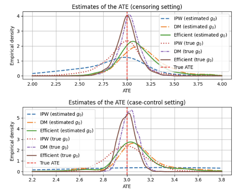
Figure 2: Empirical distributions of ATE estimates.

6 Simulation studies

This section investigates the empirical performance of the proposed estimators.

6.1 Censoring setting

We generate synthetic data under the censoring setting, where the covariates $X$ are drawn from a multivariate normal distribution as $X\sim\zeta(x)$, where $\zeta(x)$ is the density of $\mathcal{N}(0,I_{p})$, and $I_{p}$ denotes the $(p\times p)$ identity matrix. We set $p=3$. Set ${\mathbb{P}}(\widetilde{D}\mid X)=\mathrm{trunc}(\mathrm{sigmoid}(X^{\top}\beta),0.1,0.9)$, where $\beta$ is a coefficient sampled from $\mathcal{N}(0,0.5I_{p})$, and $\mathrm{trunc}(t,a,b)$ truncates $t$ by $a$ and $b$ ($a<b$). Treatment $\widetilde{D}$ is sampled from the probability. The observation indicator $O$ is generated from a Bernoulli distribution with probability $c$ if $D_{i}=1$ and $O_{i}=0$ if $D_{i}=0$. Here, $c$ is generated from a uniform distribution with support $[0,1]$. The outcome is generated as $Y=X^{\top}\beta+1.1+\tau_{0}\cdot D+\varepsilon$, where $\varepsilon\sim\mathcal{N}(0,1)$, where we set $\tau_{0}=3$.

The nuisance parameters are estimated using linear regression and (linear) logistic regression. We compared our proposed estimator, $\widehat{\tau}^{\mathrm{cens}\mathchar 45\relax\mathrm{eff}}_{n}$, with the other candidates, the IPW estimator $\widehat{\tau}^{\mathrm{cens}\mathchar 45\relax\mathrm{IPW}}_{n}$ and the DM estimator $\widehat{\tau}^{\mathrm{cens}\mathchar 45\relax\mathrm{DM}}_{n}$, defined in Remarks Remark and Remark, respectively. Note that all of these estimators are proposed by us, and our goal is not to confirm $\widehat{\tau}^{\mathrm{cens}\mathchar 45\relax\mathrm{eff}}_{n}$ outperforms the others, while our recommendation is $\widehat{\tau}^{\mathrm{cens}\mathchar 45\relax\mathrm{eff}}_{n}$. We consider both cases where the propensity score is either estimated using the method proposed by Elkan & Noto (2008) or assumed to be known.

We set $n=3000$. We conduct $5000$ trials and report the empirical mean squared errors (MSEs) and biases for the true ATE and the coverage ratio (Cov. ratio) computed from the confidence intervals in Table 1. We also present the empirical distributions of the ATE estimates in Figure 2.

As the theory suggests, $\widehat{\tau}^{\mathrm{cens}\mathchar 45\relax\mathrm{eff}}_{n}$ exhibits smaller MSEs compared to other methods. Interestingly, when the propensity score is estimated, the MSEs decrease, a phenomenon reported in existing studies. The coverage ratio is also accurate. The empirical distribution of the ATE estimates demonstrates the asymptotic normality.

6.2 Case-control setting

In the case-control setting, covariates for the treatment and unknown groups are generated from different $p$-dimensional normal distributions: $X_{{\mathrm{T}}}\sim\zeta_{{\mathrm{T}},0}(x)$ and $X\sim\zeta_{0}(x)=e_{0}(1)\zeta_{{\mathrm{T}},0}(x)+e_{0}(0)\zeta_{{\mathrm{C}}}(x)$, where we set $p=3$, $\zeta_{{\mathrm{T}},0}(x)$ and $\zeta_{{\mathrm{C}}}(x)$ are the densities of normal distributions $\mathcal{N}(\mu_{p}\bm{1}_{p},I_{p})$ and $\mathcal{N}(\mu_{n}\bm{1}_{p},I_{p})$, $\mu_{p}=0.5$ and $\mu_{n}=0$, $\bm{1}_{p}=(1\ 1\ \cdots\ 1)^{\top}$, and $e(1)$ is the class prior set as $e(1)=0.3$. By definition, the propensity score $e_{0}(d\mid x)$ is given as $e_{0}(1\mid x)=e(1)\zeta_{{\mathrm{T}},0}(x)/\zeta_{0}(x)$. The outcome is generated similarly to the censoring setting $Y=X^{\top}\beta+1.1+\tau_{0}D+\varepsilon$, where $\tau_{0}=3$.

We set $m=1000$ and $l=2000$ and compute the same evaluation metrics as in the censoring setting. Although logistic regression is used, the propensity score model is misspecified, while the expected conditional outcome follows a linear model.

Overall, $\widehat{\tau}^{\mathrm{cc}\mathchar 45\relax\mathrm{eff}}_{n}$ demonstrates robust performance in terms of MSE, bias, and coverage ratio. The poor performance of the IPW estimator is attributed to model misspecification.

We investigate non-linear settings in Appendix H.

7 Conclusion

In this study, we investigated PUATE, the problem of ATE estimation in the presence of missing treatment indicators. We formulated the problem using the censoring and case-control settings, inspired by PU learning. For each setting, we derived the efficiency bound and developed an efficient estimator. Our analysis revealed that achieving asymptotic normality and efficiency. Future research directions include extending our approach to the semi-supervised setting, handling additional missing values, and the relaxation of assumptions regarding the missingness mechanism.

Appendix A Related work

Our problem is also related to ATE estimation from misclassified data (Lewbel, 2007). Early econometric studies focused on continuous regressors (Hausman, 2001). With regard to binary variables, Mahajan (2006) analyzes misclassification in regression models, while Lewbel (2007) develops methods for identifying and estimating ATEs under potentially misclassified treatment indicators. Researchers have also explored partial identification approaches when the exact misclassification process is unknown, providing bounds on parameters rather than point estimates (Manski, 1993, 2010). In applied settings, validation data have been used to refine causal effect estimates under potential misclassification (Black et al., 2008), demonstrating that even modest errors in treatment indicators can significantly impact policy conclusions. Yamane et al. (2018) also addresses a related problem.

Finally, we refer to semi-supervised treatment effect estimation (Chakrabortty & Dai, 2024), which primarily considers a scenario where two datasets are available: one with complete data and the other with only treatment indicators $D$ and covariates $X$ but no outcome data. Although the setting is not directly related, integrating insights from both areas could enhance the applicability.

A.1 PU learning

We review representative PU learning methods. For all methods, the goal is not to obtain a conditional class probability (propensity score) but rather to obtain a better classifier. However, under specific loss functions, including logistic loss, the obtained classifiers can be interpreted as estimators of the probability (Elkan & Noto, 2008; Kato et al., 2019; Kato & Teshima, 2021).

A.1.1 Censoring PU Learning

In Elkan & Noto (2008), it is assumed that only a fraction of the truly positive instances are labeled as positive.

Let $O$ denote the event “labeled as positive,” and let $\widetilde{D}=1$ indicate true positivity. In our study, $O$ is called an observation indicator, and $\widetilde{D}$ is called a treatment indicator.

First, we make the following assumption, which plays a central role in the method of Elkan & Noto (2008):

$${\mathbb{P}}(O=1\mid\widetilde{D}=1,x)=c\Big{(}={\mathbb{P}}(O=1\mid\widetilde{D}=1)\Big{)}\ \ \ \forall x\in{\mathcal{X}},$$ (1)

where $c\in(0,1]$ is a constant (Assumption 3.3). Intuitively, $c$ represents the labeling probability or censoring rate, which denotes the fraction of positive instances that are observed (uncensored) in the labeled dataset. If we relax this assumption, we may not pointy identify the ATE without different assumptions. There are various approaches proposed to address the relaxation (Bekker & Davis, 2018).

The learning procedure proposed by Elkan & Noto (2008) consists of three main steps (for details, see Elkan & Noto (2008)):

Estimation of $\pi_{0}$:

First, the observation probability $\pi_{0}$ is estimated using standard regression methods, such as logistic regression.

Estimation of $c$:

Next, $c$ is estimated using an estimator $\widehat{\pi}_{n}$ of $\pi_{0}$. Under Assumption 3.3, $c$ can be estimated by taking the sample average of $\widehat{\pi}_{n}$ over positively labeled samples.

Correction of the observation probability:

From Assumption 3.3, we have $\pi_{0}(1\mid X)=c{\mathbb{P}}(\widetilde{D}=1\mid X)$. Using this relationship and the estimators of $\pi_{0}$ and $c$, ${\mathbb{P}}(\widetilde{D}=1\mid X)$ is estimated as $\widehat{\pi}_{n}(1\mid X)/\widehat{c}$.

A.1.2 Case-Control PU Learning

A different perspective is provided by du Plessis et al. (2015) and subsequent studies, often referred to as case-control PU learning. In this approach, the labeled positive data follows a distribution $\zeta_{{\mathrm{T}}}(x)$, whereas the unlabeled data is generated from $\zeta(x)$, a mixture of positives and negatives.

Let $h$ be a classifier. In conventional supervised learning, the classification risk is defined as:

$$R(h)=e_{0}(1)R_{+}(h,+1)+(1-e_{0}(1))R_{-}(h,-1),$$

where $e_{0}(1)$ is the prior probability of being positive, and $R_{+}(h,+1)$ and $R_{-}(h,-1)$ represent the risks over the positive and negative distributions, respectively. The risk $R_{+}(h,+1)$ corresponds to the expected loss when predicting class $-1$ while the true label is $+1$ in the positive distribution, whereas $R_{-}(h,-1)$ represents the expected loss when predicting class $+1$ while the true label is $-1$ in the negative distribution.

Since negative examples are unavailable, du Plessis et al. (2015) re-expresses $R_{-}(h,-1)$ as:

$$(1-e_{0}(1))R_{-}(h,-1)=R_{{\mathrm{U}}}(h,-1)-e_{0}(1)R_{+}(h,-1),$$

where $R_{{\mathrm{U}}}(h,-1)$ and $R_{+}(h,-1)$ represent the risks over the unlabeled and positive distributions, respectively. The risk $R_{{\mathrm{U}}}(h,-1)$ corresponds to the expected loss when predicting class $+1$ while the true label is $-1$ in the unlabeled distribution, whereas $R_{+}(h,-1)$ represents the expected loss when predicting class $+1$ while the true label is $-1$ in the positive distribution. Note that $R_{+}(h,+1)$ and $R_{+}(h,-1)$ are distinct, as they consider different labels to be true while the expectation is taken over the same positively labeled distributions. The sample approximation of this risk formulation is referred to as an unbiased risk estimator.

A.2 Density-Ratio Estimation

Since the density ratio can be estimated in the case-control setting, we introduce related methods. Density-ratio estimation has emerged as a powerful technique in machine learning and statistics, providing a principled approach for estimating the ratio of two probability density functions (Sugiyama et al., 2012). Let $X_{i},Z_{i}\in{\mathcal{X}}$ be random variables. Specifically, if $\{X_{i}\}_{i=1}^{n}$ are drawn from $p_{0}(x)$ and $\{Z_{j}\}_{j=1}^{m}$ are drawn from $q_{0}(z)$, the goal is to estimate

$$r_{0}(x)=\frac{p_{0}(x)}{q_{0}(x)}$$

directly, without first estimating $p_{0}(x)$ and $q_{0}(z)$ separately.

Estimating $p_{0}(x)$ and $q_{0}(z)$ individually can be challenging and may introduce unnecessary modeling complexities if only the ratio $r_{0}(x)$ is required. By directly estimating the density ratio, more stable and accurate estimates can often be obtained, avoiding potential compounding errors from separately learned density models.

Various algorithms have been proposed for direct density-ratio estimation, including the Kullback–Leibler Importance Estimation Procedure (KLIEP, Sugiyama et al., 2008) and Least-Squares Importance Fitting (LSIF, Kanamori et al., 2009). These methods typically optimize a criterion that ensures the estimated ratio closely approximates the true ratio in a specific divergence sense, such as the Kullback–Leibler divergence or squared error, which can be generalized as a Bregman divergence minimization problem (Sugiyama et al., 2012).

From the Bregman divergence minimization perspective, PU learning methods can also be seen as variants of density-ratio estimation, as demonstrated in Kato et al. (2019) and Kato & Teshima (2021).

Appendix B Remarks on the nuisance parameter estimation in the censoring setting

In the censoring setting, by applying the method of Elkan & Noto (2008), we can obtain an estimator of ${\mathbb{P}}(\widetilde{D}=1\mid X)$ from an estimator of $\pi_{0}(x)={\mathbb{P}}(O=1\mid X)$. However, our objective is to estimate $g_{0}(1\mid X){\mathbb{P}}(\widetilde{D}=1\mid X,O=0)$ rather than ${\mathbb{P}}(\widetilde{D}=1\mid X)$.

Let $\widehat{\kappa}_{n}(1\mid X)$ be an estimator of ${\mathbb{P}}(\widetilde{D}=1\mid X)$. We can then obtain an estimator of $g_{0}(1\mid X)$ as follows:

$$\widehat{g}_{n}(1\mid X)=\frac{(1-\widehat{c})\widehat{\kappa}_{n}(1\mid X)}{\widehat{\pi}_{n}(0\mid X)}=\frac{(1-\widehat{c})\widehat{\pi}_{n}(0\mid X)}{\widehat{c}\widehat{\pi}_{n}(0\mid X)},$$

where $\widehat{c}$ is an estimate of $c={\mathbb{P}}(O=0\mid\widetilde{D}=1)$. Notably, under Assumption 3.3, $c$ can be estimated by taking the mean of $\widehat{\pi}_{n}(0\mid X)$ over the positively labeled sample ($O_{i}=1$).

Appendix C Pseudo-code for ATE estimation in the case-control setting

We explain how we construct the estimators of the nuisance parameters in the case-control setting.

We can estimate $\mu_{{\mathrm{T}},0}$ and $\mu_{{\mathrm{U}},0}$ using standard regression methods, including logistic regression and nonparametric regression. Specifically, for estimating $\mu_{{\mathrm{T}},0}$, we typically use the dataset $\left\{\big{(}X_{{\mathrm{T}},j},Y_{j}(1)\big{)}\right\}^{m}_{j=1}$, while for estimating $\mu_{{\mathrm{U}},0}$, we use $\left\{\big{(}X_{k},Y_{{\mathrm{U}},k}\big{)}\right\}^{l}_{k=1}$.

To estimate $e_{0}$, we can apply case-control PU learning methods, such as convex PU learning proposed by du Plessis et al. (2015). For estimating $r_{0}$, density-ratio estimation methods can be employed (Sugiyama et al., 2012).

Notably, if $\zeta_{{\mathrm{T}},0}(x)=\zeta_{0}(x\mid d=1)$, then $r_{0}$ can be estimated from an estimator of $e_{0}$ using the relationship $r_{0}=1/(e_{0}(1\mid x)e_{0}(1))$.

In cross-fitting, we split ${\mathcal{D}}_{{\mathrm{T}}}$ and ${\mathcal{D}}_{{\mathrm{U}}}$, respectively, as performed in Uehara et al. (2020). The pseudo-code is shown in Algorithm 2.

Algorithm 2 Cross-fitting in the case-control setting

 Input: Observations ${\mathcal{D}}_{{\mathrm{T}}}=\left\{\big{(}X_{{\mathrm{T}},j},Y_{j}(1)\big{)}\right\}^{m}_{j=1}$ and ${\mathcal{D}}_{{\mathrm{U}}}=\left\{\big{(}X_{k},Y_{{\mathrm{U}},k}\big{)}\right\}^{l}_{k=1}$, number of folds $L$, and estimation methods for $\mu_{{\mathrm{T}},0},\mu_{{\mathrm{U}},0},e_{0},r_{0}$.

 Randomly partition ${\mathcal{D}}_{{\mathrm{T}}}$ into $L$ roughly equal-sized folds, $(\mathcal{J}^{(\ell)})_{\ell\in{\mathcal{L}}}$. Note that $\bigcup_{\ell\in{\mathcal{L}}}{\mathcal{J}}^{(\ell)}={\mathcal{D}}$.

 Randomly partition ${\mathcal{D}}_{{\mathrm{U}}}$ into $L$ roughly equal-sized folds, $(\mathcal{K}^{(\ell)})_{\ell\in{\mathcal{L}}}$. Note that $\bigcup_{\ell\in{\mathcal{L}}}{\mathcal{K}}^{(\ell)}={\mathcal{D}}$.

 for $\ell\in{\mathcal{L}}$ do

  Set the training data as $\mathcal{J}^{(-\ell)}=\{1,2,\dots,n\}\setminus\mathcal{J}^{(\ell)}$.

  Set the training data as $\mathcal{K}^{(-\ell)}=\{1,2,\dots,n\}\setminus\mathcal{K}^{(\ell)}$.

  Construct estimators of nuisance parameters on $\mathcal{J}^{(-\ell)}$ and $\mathcal{K}^{(-\ell)}$.

  Construct an ATE estimate $\widehat{\tau}^{\mathrm{cc}\mathchar 45\relax\mathrm{eff}(\ell)}_{n}$ using $\mathcal{J}^{(\ell)}$, $\mathcal{K}^{(\ell)}$and the nuisance estimates $\widehat{\mu}^{(\ell)}_{{\mathrm{T}},n},\widehat{\mu}^{(\ell)}_{{\mathrm{U}},n},\widehat{e}^{(\ell)}_{n},\widehat{r}^{(\ell)}_{n}$.

 end for

 Output: Combine $(\widehat{\tau}^{\mathrm{cc}\mathchar 45\relax\mathrm{eff}(\ell)}_{n})_{\ell\in{\mathcal{L}}}$ to form $\widehat{\tau}^{\mathrm{cc}\mathchar 45\relax\mathrm{eff}}_{n}$.

Appendix D Proof of Lemma 4.1

We prove Lemma 4.1. Our proof procedure is inspired by the one in Hahn (1998).

Proof.

Recall that the density function for $(X,O,Y)$ is given as

$$p(x,o,y)=\zeta(x)\Big{(}\pi(1\mid x)p_{Y(1)}(y\mid x)\Big{)}^{\mathbbm{1}[o=1]}\Big{(}\pi(0\mid x)p_{\widetilde{Y}}(y\mid x)\Big{)}^{\mathbbm{1}[o=0]}$$

For this density function, we consider the parametric submodels:

$${\mathcal{P}}^{\mathrm{sub}}\coloneqq\{P_{\theta}\coloneqq\theta\in{\mathbb{R}},$$

where $P_{\theta}$ has the following density:

$$p(x,o,y;\theta)=\zeta(x;\theta)\Big{(}\pi(1\mid x;\theta)p_{Y(1)}(y\mid x;\theta)\Big{)}^{\mathbbm{1}[o=1]}\Big{(}\pi(0\mid x;\theta)p_{\widetilde{Y}}(y\mid x;\theta)\Big{)}^{\mathbbm{1}[o=0]},$$

while there exists $\theta_{0}\in{\mathbb{R}}$ such that

$$p(x,o,y;\theta_{0})=p_{0}(x,o,y).$$

Then, we define scores as follows:

$$S(x,o,y;\theta) \coloneqq\frac{\partial}{\partial\theta}\log p(x,o,y;\theta)$$

$$=S_{X}(x;\theta)+\mathbbm{1}[o=1]\left(S_{Y(1)}(y\mid x;\theta)+\frac{\dot{\pi}(1\mid x;\theta)}{\pi(1\mid x;\theta)}\right)+\mathbbm{1}[o=0]\left(S_{\widetilde{Y}}(y\mid x;\theta)+\frac{\dot{\pi}(0\mid x;\theta)}{\pi(0\mid x;\theta)}\right),$$

where

$$S_{X}(x;\theta) \coloneqq\frac{d}{d\theta}\log\zeta(x;\theta),$$

$$S_{Y(1)}(y\mid x;\theta) \coloneqq\frac{d}{d\theta}\log p_{Y(1)}(y\mid x;\theta),$$

$$S_{\widetilde{Y}}(y\mid x;\theta) \coloneqq\frac{d}{d\theta}\log p_{\widetilde{Y}}(y\mid x;\theta),$$

$$\dot{\pi}(0\mid x;\theta) \coloneqq\frac{d}{d\theta}\pi(o\mid x;\theta),$$

Let ${\mathcal{T}}\coloneqq\{S(x,o,y;\theta)\}$ be the tangent space.

Here, note that

$$p_{\widetilde{Y}}(y\mid x)=g_{0}(1\mid x)p_{Y(1)}(y\mid x)+g_{0}(0\mid x)p_{Y(0)}(y\mid x).$$

We have

$$p_{Y(0)}(y\mid x)=\frac{1}{g_{0}(0\mid x)}\Big{(}p_{\widetilde{Y}}(y\mid x)-g_{0}(1\mid x)p_{Y(1)}(y\mid x)\Big{)}$$

Using this relationship, we write the ATE under the parametric submodels as

$$\tau(\theta) \coloneqq\iint y(1)p_{Y(1)}(y(1)\mid x;\theta)\zeta(x;\theta){\mathrm{d}}y(1){\mathrm{d}}x-\iint y(0)p_{Y(0)}(y(0)\mid x;\theta)\zeta(x;\theta){\mathrm{d}}y(0){\mathrm{d}}x$$

$$=\iint y(1)p_{Y(1)}(y(1)\mid x;\theta)\zeta(x;\theta){\mathrm{d}}y(1){\mathrm{d}}x-\iint y(0)\frac{1}{g_{0}(0\mid x)}p_{\widetilde{Y}}(y(0)\mid x;\theta)\zeta(x;\theta){\mathrm{d}}y(0){\mathrm{d}}x$$

$$\ \ \ \ \ \ \ \ \ \ \ \ \ \ \ \ \ \ \ \ \ \ \ \ \ \ \ \ \ \ \ \ \ \ \ \ \ \ \ \ \ \ \ \ \ \ \ \ \ \ \ \ \ \ \ \ \ \ \ \ +\iint y(0)\frac{g_{0}(1\mid x)}{g_{0}(0\mid x)}p_{Y(1)}(y(0)\mid x;\theta)\zeta(x;\theta){\mathrm{d}}y(0){\mathrm{d}}x.$$

Them, the derivative is given as

$$\frac{\partial\tau(\theta)}{\partial\theta} ={\mathbb{E}}_{\theta}\Big{[}Y(1)S_{Y(1)}(Y(1)\mid X;\theta)\Big{]}-{\mathbb{E}}_{\theta}\left[\frac{1}{g_{0}(0\mid X)}\widetilde{Y}S_{\widetilde{Y}}(\widetilde{Y}\mid X;\theta)\right]$$

$$\ \ \ +{\mathbb{E}}_{\theta}\left[\frac{g_{0}(1\mid X)}{g_{0}(0\mid X)}Y(1)S_{Y(1)}(Y(1)\mid X;\theta)\right]$$

$$\ \ \ +{\mathbb{E}}_{\theta}\Big{[}\tau(X;\theta)S_{X}(X;\theta)\Big{]},$$

where

$$\tau(X;\theta)\coloneqq\mu(1\mid X)-\frac{1}{g_{0}(0\mid X)}\mu(U\mid X)+\frac{g_{0}(1\mid X)}{g_{0}(0\mid X)}\mu(1\mid X)=\mu(1\mid X)-\mu(0\mid X)$$

From the Riesz representation theorem, there exists a function $\Psi$ such that

$$\frac{\partial\tau(\theta)}{\partial\theta}\Big{|}_{\theta=\theta_{0}}={\mathbb{E}}\big{[}\Psi(X,O,Y)S(X,O,Y;\theta_{0})\big{]}.$$ (2)

There exists a unique function $\Psi^{\mathrm{cens}}$ such that $\Psi^{\mathrm{cens}}\in{\mathcal{T}}$, called the efficient influence function. We specify the efficient influence function as

$$\Psi^{\mathrm{cens}}(X,O,Y;\mu_{{\mathrm{T}},0},\nu_{0},\pi_{0},g_{0}) =S^{\mathrm{cens}}(X,O,Y;\mu_{{\mathrm{T}},0},\nu_{0},\pi_{0},g_{0})-\tau_{0},$$

$$=\frac{\mathbbm{1}[O=1]\Big{(}Y-\mu_{{\mathrm{T}},0}(X)\Big{)}}{\pi_{0}(1\mid X)}-\frac{\mathbbm{1}[O=0]\Big{(}Y-\nu_{0}(X)\Big{)}}{g_{0}(0\mid X)\pi_{0}(0\mid X)}$$

$$\ \ \ +\frac{g(1\mid X)\mathbbm{1}[O=1]\Big{(}Y-\mu_{{\mathrm{T}},0}(X)\Big{)}}{g_{0}(0\mid X)\pi_{0}(1\mid X)}$$

$$\ \ \ +\mu_{{\mathrm{T}},0}(X)-\frac{1}{g_{0}(0\mid X)}\nu(X)+\frac{g_{0}(1\mid X)}{g_{0}(0\mid X)}\mu_{{\mathrm{T}},0}(X)-\tau_{0}.$$

We prove that $\Psi^{\mathrm{cens}}(X,O,Y;\mu_{{\mathrm{T}},0},\nu_{0},\pi_{0},g_{0})$ is actually the unique efficient influence function by verifying that $\Psi^{\mathrm{cens}}$ satisfies (2) and $\Psi^{\mathrm{cens}}\in{\mathcal{T}}$.

Proof of (2):

First, we confirm that $\Psi^{\mathrm{cens}}$ satisfies (2). We have

$${\mathbb{E}}\left[\Psi^{\mathrm{cens}}(X,O,Y;\mu_{{\mathrm{T}},0},\nu_{0},\pi_{0},g_{0})S(X,O,Y;\theta_{0})\right]$$

$$={\mathbb{E}}\Bigg{[}\Psi^{\mathrm{cens}}(X,O,Y;\mu_{{\mathrm{T}},0},\nu_{0},\pi_{0},g_{0})$$

$$\ \ \ \ \cdot\left(S_{X}(X;\theta)+\mathbbm{1}[O=1]\left(S_{Y(1)}(Y\mid X;\theta)+\frac{\dot{\pi}(1\mid X;\theta)}{\pi(1\mid X;\theta_{0})}\right)+\mathbbm{1}[O=0]\left(S_{\widetilde{Y}}(Y\mid X;\theta)+\frac{\dot{\pi}(0\mid X;\theta_{0})}{\pi(0\mid X;\theta_{0})}\right)\right)\Bigg{]}$$

$$={\mathbb{E}}\Bigg{[}\Bigg{(}\frac{\mathbbm{1}[O=1]\Big{(}Y-\mu_{{\mathrm{T}},0}(X)\Big{)}}{\pi_{0}(1\mid X)}-\frac{\mathbbm{1}[O=0]\Big{(}Y-\nu_{0}(X)\Big{)}}{g_{0}(0\mid X)\pi_{0}(0\mid X)}$$

$$\ \ \ \ \ \ +\frac{g(1\mid X)\mathbbm{1}[O=1]\Big{(}Y-\mu_{{\mathrm{T}},0}(X)\Big{)}}{g_{0}(0\mid X)\pi_{0}(1\mid X)}$$

$$\ \ \ \ \ \ +\mu_{{\mathrm{T}},0}(X)-\frac{1}{g_{0}(0\mid X)}\nu(X)+\frac{g_{0}(1\mid X)}{g_{0}(0\mid X)}\mu_{{\mathrm{T}},0}(X)-\tau_{0}\Bigg{)}$$

$$\ \ \ \ \cdot\left(S_{X}(X;\theta)+\mathbbm{1}[O=1]\left(S_{Y(1)}(Y\mid X;\theta)+\frac{\dot{\pi}(1\mid X;\theta)}{\pi(1\mid X;\theta_{0})}\right)+\mathbbm{1}[O=0]\left(S_{\widetilde{Y}}(Y\mid X;\theta)+\frac{\dot{\pi}(0\mid X;\theta_{0})}{\pi(0\mid X;\theta_{0})}\right)\right)\Bigg{]}$$

$$={\mathbb{E}}\Bigg{[}\Bigg{(}\mu_{{\mathrm{T}},0}(X)-\frac{1}{g_{0}(0\mid X)}\nu(X)+\frac{g_{0}(1\mid X)}{g_{0}(0\mid X)}\mu_{{\mathrm{T}},0}(X)-\tau_{0}\Bigg{)}S_{X}(X;\theta)$$

$$\ \ \ \ +\Bigg{(}\frac{\mathbbm{1}[O=1]\Big{(}Y-\mu_{{\mathrm{T}},0}(X)\Big{)}}{\pi_{0}(1\mid X)}+\frac{g(1\mid X)\mathbbm{1}[O=1]\Big{(}Y-\mu_{{\mathrm{T}},0}(X)\Big{)}}{g_{0}(0\mid X)\pi_{0}(1\mid X)}$$

$$\ \ \ \ \ \ +\mu_{{\mathrm{T}},0}(X)-\frac{1}{g_{0}(0\mid X)}\nu(X)+\frac{g_{0}(1\mid X)}{g_{0}(0\mid X)}\mu_{{\mathrm{T}},0}(X)-\tau_{0}\Bigg{)}\mathbbm{1}[O=1]\left(S_{Y(1)}(Y\mid X;\theta)+\frac{\dot{\pi}(1\mid X;\theta)}{\pi(1\mid X;\theta_{0})}\right)$$

$$\ \ \ \ \ \ +\Bigg{(}-\frac{\mathbbm{1}[O=0]\Big{(}Y-\nu_{0}(X)\Big{)}}{g_{0}(0\mid X)\pi_{0}(0\mid X)}+\mu_{{\mathrm{T}},0}(X)-\frac{1}{g_{0}(0\mid X)}\nu(X)+\frac{g_{0}(1\mid X)}{g_{0}(0\mid X)}\mu_{{\mathrm{T}},0}(X)-\tau_{0}\Bigg{)}$$

$$\ \ \ \ \ \ \ \ \ \ \ \cdot\mathbbm{1}[O=0]\left(S_{\widetilde{Y}}(Y\mid X;\theta)+\frac{\dot{\pi}(0\mid X;\theta_{0})}{\pi(0\mid X;\theta_{0})}\right)\Bigg{]},$$

where we used $\mathbbm{1}[O=1]\mathbbm{1}[O=0]=0$, and

$${\mathbb{E}}\Bigg{[}\frac{\mathbbm{1}[O=1]\Big{(}Y-\mu_{{\mathrm{T}},0}(X)\Big{)}}{\pi_{0}(1\mid X)}\Bigg{]}={\mathbb{E}}\Bigg{[}\frac{\mathbbm{1}[O=1]\Big{(}Y(1)-\mu_{{\mathrm{T}},0}(X)\Big{)}}{\pi_{0}(1\mid X)}\Bigg{]}={\mathbb{E}}\Bigg{[}\frac{\pi_{0}(1\mid X)\Big{(}\mu_{{\mathrm{T}},0}(X)-\mu_{{\mathrm{T}},0}(X)\Big{)}}{\pi_{0}(1\mid X)}\Bigg{]}=0,$$

$${\mathbb{E}}\Bigg{[}\frac{\mathbbm{1}[O=0]\Big{(}Y-\nu_{0}(X)\Big{)}}{g_{0}(0\mid X)\pi_{0}(0\mid X)}\Bigg{]}={\mathbb{E}}\Bigg{[}\frac{\mathbbm{1}[O=0]\Big{(}\widetilde{Y}-\nu_{0}(X)\Big{)}}{g_{0}(0\mid X)\pi_{0}(0\mid X)}\Bigg{]}={\mathbb{E}}\Bigg{[}\frac{\pi_{0}(0\mid X)\Big{(}\nu_{0}(X)-\nu_{0}(X)\Big{)}}{g_{0}(0\mid X)\pi_{0}(0\mid X)}\Bigg{]}=0,$$

$${\mathbb{E}}\Bigg{[}\frac{g(1\mid X)\mathbbm{1}[O=1]\Big{(}Y-\mu_{{\mathrm{T}},0}(X)\Big{)}}{g_{0}(0\mid X)\pi_{0}(1\mid X)}\Bigg{]}={\mathbb{E}}\Bigg{[}\frac{g(1\mid X)\pi_{0}(1\mid X)\Big{(}\mu_{{\mathrm{T}},0}(X)-\mu_{{\mathrm{T}},0}(X)\Big{)}}{g_{0}(0\mid X)\pi_{0}(1\mid X)}\Bigg{]}=0.$$

We have

$${\mathbb{E}}\Bigg{[}\Bigg{(}\mu_{{\mathrm{T}},0}(X)-\frac{1}{g_{0}(0\mid X)}\nu(X)+\frac{g_{0}(1\mid X)}{g_{0}(0\mid X)}\mu_{{\mathrm{T}},0}(X)-\tau_{0}\Bigg{)}S_{X}(X;\theta)$$

$$\ \ \ \ +\Bigg{(}\frac{\mathbbm{1}[O=1]\Big{(}Y-\mu_{{\mathrm{T}},0}(X)\Big{)}}{\pi_{0}(1\mid X)}+\frac{g(1\mid X)\mathbbm{1}[O=1]\Big{(}Y-\mu_{{\mathrm{T}},0}(X)\Big{)}}{g_{0}(0\mid X)\pi_{0}(1\mid X)}$$

$$\ \ \ \ \ \ +\mu_{{\mathrm{T}},0}(X)-\frac{1}{g_{0}(0\mid X)}\nu(X)+\frac{g_{0}(1\mid X)}{g_{0}(0\mid X)}\mu_{{\mathrm{T}},0}(X)-\tau_{0}\Bigg{)}\mathbbm{1}[O=1]\left(S_{Y(1)}(Y\mid X;\theta)+\frac{\dot{\pi}(1\mid X;\theta)}{\pi(1\mid X;\theta_{0})}\right)$$

$$\ \ \ \ \ \ +\Bigg{(}-\frac{\mathbbm{1}[O=0]\Big{(}Y-\nu_{0}(X)\Big{)}}{g_{0}(0\mid X)\pi_{0}(0\mid X)}+\mu_{{\mathrm{T}},0}(X)-\frac{1}{g_{0}(0\mid X)}\nu(X)+\frac{g_{0}(1\mid X)}{g_{0}(0\mid X)}\mu_{{\mathrm{T}},0}(X)-\tau_{0}\Bigg{)}$$

$$\ \ \ \ \ \ \ \ \ \ \ \cdot\mathbbm{1}[O=0]\left(S_{\widetilde{Y}}(Y\mid X;\theta)+\frac{\dot{\pi}(0\mid X;\theta_{0})}{\pi(0\mid X;\theta_{0})}\right)\Bigg{]}$$

$$={\mathbb{E}}\Bigg{[}\Bigg{(}\mu_{{\mathrm{T}},0}(X)-\frac{1}{g_{0}(0\mid X)}\nu(X)+\frac{g_{0}(1\mid X)}{g_{0}(0\mid X)}\mu_{{\mathrm{T}},0}(X)\Bigg{)}S_{X}(X;\theta)$$

$$\ \ \ \ +\Bigg{(}\frac{\mathbbm{1}[O=1]\Big{(}Y-\mu_{{\mathrm{T}},0}(X)\Big{)}}{\pi_{0}(1\mid X)}+\frac{g(1\mid X)\mathbbm{1}[O=1]\Big{(}Y-\mu_{{\mathrm{T}},0}(X)\Big{)}}{g_{0}(0\mid X)\pi_{0}(1\mid X)}\Bigg{)}S_{Y(1)}(Y\mid X;\theta)$$

$$\ \ \ \ \ \ -\frac{\mathbbm{1}[O=0]\Big{(}Y-\nu_{0}(X)\Big{)}}{g_{0}(0\mid X)\pi_{0}(0\mid X)}S_{\widetilde{Y}}(Y\mid X;\theta)\Bigg{]}$$

$$={\mathbb{E}}\Bigg{[}\Bigg{(}\mu_{{\mathrm{T}},0}(X)-\frac{1}{g_{0}(0\mid X)}\nu(X)+\frac{g_{0}(1\mid X)}{g_{0}(0\mid X)}\mu_{{\mathrm{T}},0}(X)\Bigg{)}S_{X}(X;\theta)$$

$$\ \ \ \ +\Bigg{(}\frac{\mathbbm{1}[O=1]Y(1)}{\pi_{0}(1\mid X)}+\frac{g(1\mid X)\mathbbm{1}[O=1]Y(1)}{g_{0}(0\mid X)\pi_{0}(1\mid X)}\Bigg{)}S_{Y(1)}(Y(1)\mid X;\theta)-\frac{\mathbbm{1}[O=0]\widetilde{Y}}{g_{0}(0\mid X)\pi_{0}(0\mid X)}S_{\widetilde{Y}}(\widetilde{Y}\mid X;\theta)\Bigg{]},$$

where we used

$${\mathbb{E}}\Bigg{[}\tau_{0}S_{X}(X;\theta)\Bigg{]}=0$$

$${\mathbb{E}}\Bigg{[}\Big{(}\mu_{{\mathrm{T}},0}(X)-\frac{1}{g_{0}(0\mid X)}\nu(X)+\frac{g_{0}(1\mid X)}{g_{0}(0\mid X)}\mu_{{\mathrm{T}},0}(X)-\tau_{0}\Big{)}\mathbbm{1}[O=1]\left(S_{Y(1)}(Y\mid X;\theta)+\frac{\dot{\pi}(1\mid X;\theta)}{\pi(1\mid X;\theta_{0})}\right)\Bigg{]}=0.$$

Finally, we have

$${\mathbb{E}}\Bigg{[}\Bigg{(}\mu_{{\mathrm{T}},0}(X)-\frac{1}{g_{0}(0\mid X)}\nu(X)+\frac{g_{0}(1\mid X)}{g_{0}(0\mid X)}\mu_{{\mathrm{T}},0}(X)\Bigg{)}S_{X}(X;\theta)$$

$$\ \ \ \ +\Bigg{(}\frac{\mathbbm{1}[O=1]Y(1)}{\pi_{0}(1\mid X)}+\frac{g(1\mid X)\mathbbm{1}[O=1]Y(1)}{g_{0}(0\mid X)\pi_{0}(1\mid X)}\Bigg{)}S_{Y(1)}(Y(1)\mid X;\theta)-\frac{\mathbbm{1}[O=0]\widetilde{Y}}{g_{0}(0\mid X)\pi_{0}(0\mid X)}S_{\widetilde{Y}}(\widetilde{Y}\mid X;\theta)\Bigg{]}$$

$$={\mathbb{E}}_{\theta}\Big{[}Y(1)S_{Y(1)}(Y(1)\mid X;\theta)\Big{]}-{\mathbb{E}}_{\theta}\left[\frac{1}{g_{0}(0\mid X)}\widetilde{Y}S_{\widetilde{Y}}(\widetilde{Y}\mid X;\theta)\right]$$

$$\ \ \ +{\mathbb{E}}_{\theta}\left[\frac{g_{0}(1\mid X)}{g_{0}(0\mid X)}Y(1)S_{Y(1)}(Y(1)\mid X;\theta)\right]$$

$$\ \ \ +{\mathbb{E}}_{\theta}\Big{[}\tau(X;\theta)S_{X}(X;\theta)\Big{]}$$

$$=\frac{\partial\tau(\theta)}{\partial\theta}$$

Proof of $\Psi^{\mathrm{cens}}\in{\mathcal{T}}$:

Set

$$S_{Y(1)}(y\mid x)=\frac{y-{\mathbb{E}}\big{[}Y(1)\mid X=x\big{]}}{\pi(1\mid x)},$$

$$S_{\widetilde{Y}}(y\mid x)=\frac{y-{\mathbb{E}}\big{[}\widetilde{Y}\mid X=x\big{]}}{\pi(0\mid x)},$$

$$S_{X}(X;\theta)=\mu_{{\mathrm{T}},0}(X)-\frac{1}{g_{0}(0\mid X)}\nu(X)+\frac{g_{0}(1\mid X)}{g_{0}(0\mid X)}\mu_{{\mathrm{T}},0}(X)-\tau_{0}.$$

Then, $\Psi^{\mathrm{cens}}\in{\mathcal{T}}$ holds. ∎

Appendix E Proof of Theorem 4.7: Semiparametric efficient ATE estimator under the censoring setting

For simplicity, we consider two-fold cross-fitting; that is, $L=2$. Without loss of generality, we assume that the sample size $n$ is even, and let $\overline{n}=n/2$. For each $\ell\in\{1,2\}$, we denote the subset of the dataset in cross-fitting as

$${\mathcal{I}}^{(\ell)}\coloneqq\{(\widetilde{X}^{\ell}_{i},\widetilde{O}^{(\ell)}_{i},\widetilde{Y}^{(\ell)}_{i})\}^{\overline{n}}_{i=1}.$$

We defined the estimator as

$$\widehat{\tau}^{\mathrm{cens}\mathchar 45\relax\mathrm{eff}}_{n}\coloneqq\frac{1}{n}\sum^{n}_{i=1}S^{\mathrm{cens}}(X_{i},O_{i},Y_{i};\widehat{\mu}_{{\mathrm{T}},n,i},\widehat{\nu}_{n,i},\widehat{\pi}_{n,i},g_{0}),$$

where recall that

$$S^{\mathrm{cens}}(X,O,Y;\mu_{{\mathrm{T}}},\nu,\pi,e) =\frac{\mathbbm{1}[O=1]\Big{(}Y-\mu_{{\mathrm{T}}}(X)\Big{)}}{\pi(1\mid X)}-\frac{\mathbbm{1}[O=0]\Big{(}Y-\nu(X)\Big{)}}{g(0\mid X)\pi(0\mid X)}+\frac{g(1\mid X)\mathbbm{1}[O=1]\Big{(}Y-\mu_{{\mathrm{T}}}(X)\Big{)}}{g(0\mid X)\pi(1\mid X)}$$

$$\ \ \ +\mu_{{\mathrm{T}}}(X)-\frac{1}{g(0\mid X)}\nu(X)+\frac{g(1\mid X)}{g(0\mid X)}\mu_{{\mathrm{T}}}(X).$$

We have

$$\widehat{\tau}^{\mathrm{cens}\mathchar 45\relax\mathrm{eff}}_{n} =\frac{1}{n}\sum^{n}_{i=1}S^{\mathrm{cens}}(X_{i},O_{i},Y_{i};\widehat{\mu}_{{\mathrm{T}},n,i},\widehat{\nu}_{n,i},\widehat{\pi}_{n,i},g_{0})$$

$$=\frac{1}{n}\sum^{n}_{i=1}S^{\mathrm{cens}}(X_{i},O_{i},Y_{i};\mu_{{\mathrm{T}},0},\nu_{0},\pi_{0},g_{0})-\frac{1}{n}\sum^{n}_{i=1}S^{\mathrm{cens}}(X_{i},O_{i},Y_{i};\mu_{{\mathrm{T}},0},\nu_{0},\pi_{0},g_{0})$$

$$\ \ \ \ \ \ +\frac{1}{n}\sum^{n}_{i=1}S^{\mathrm{cens}}(X_{i},O_{i},Y_{i};\widehat{\mu}_{{\mathrm{T}},n,i},\widehat{\nu}_{n,i},\widehat{\pi}_{n,i},g_{0}).$$

Here, if it holds that

$$\frac{1}{n}\sum^{n}_{i=1}S^{\mathrm{cens}}(X_{i},O_{i},Y_{i};\mu_{{\mathrm{T}},0},\nu_{0},\pi_{0},g_{0})-\frac{1}{n}\sum^{n}_{i=1}S^{\mathrm{cens}}(X_{i},O_{i},Y_{i};\widehat{\mu}_{{\mathrm{T}},n,i},\widehat{\nu}_{n,i},\widehat{\pi}_{n,i},g_{0})=o_{p}(1/\sqrt{n})$$ (3)

then we have

$$\sqrt{n}\Big{(}\widehat{\tau}^{\mathrm{cens}\mathchar 45\relax\mathrm{eff}}_{n}-\tau_{0}\Big{)} =\frac{1}{\sqrt{n}}\sum^{n}_{i=1}S^{\mathrm{cens}}(X_{i},O_{i},Y_{i};\mu_{{\mathrm{T}},0},\nu_{0},\pi_{0},g_{0})+o_{p}(1)$$

$$\xrightarrow{{\mathrm{d}}}\mathcal{N}(0,V^{\mathrm{cens}}),$$

from the central limit theorem for i.i.d. random variables.

Therefore, we prove Theorem 4.7 by showing (3). We decompose the LHS of (3) as

$$\frac{1}{n}\sum^{n}_{i=1}S^{\mathrm{cens}}(X_{i},O_{i},Y_{i};\mu_{{\mathrm{T}},0},\nu_{0},\pi_{0},g_{0})-\frac{1}{n}\sum^{n}_{i=1}S^{\mathrm{cens}}(X_{i},O_{i},Y_{i};\widehat{\mu}_{{\mathrm{T}},n,i},\widehat{\nu}_{n,i},\widehat{\pi}_{n,i},g_{0})$$

$$=\frac{\overline{n}}{n}\sum_{\ell\in\{1,2\}}\Bigg{(}\frac{1}{\overline{n}}\sum^{m}_{i=1}S^{\mathrm{cens}}(\widetilde{X}^{(\ell)}_{i},\widetilde{O}^{(\ell)}_{i},\widetilde{Y}^{(\ell)}_{i};\mu_{{\mathrm{T}},0},\nu_{0},\pi_{0},g_{0})-\frac{1}{\overline{n}}\sum^{m}_{i=1}S^{\mathrm{cens}}(\widetilde{X}^{(\ell)}_{i},\widetilde{O}^{(\ell)}_{i},\widetilde{Y}^{(\ell)}_{i};\widehat{\mu}^{(\ell)}_{{\mathrm{T}},n},\widehat{\nu}^{(\ell)}_{n},\widehat{\pi}^{(\ell)}_{n},g_{0})\Bigg{)}.$$

Here, we have

$$\frac{1}{\overline{n}}\sum^{m}_{i=1}S^{\mathrm{cens}}(\widetilde{X}^{(\ell)}_{i},\widetilde{O}^{(\ell)}_{i},\widetilde{Y}^{(\ell)}_{i};\mu_{{\mathrm{T}},0},\nu_{0},\pi_{0},g_{0})-\frac{1}{\overline{n}}\sum^{m}_{i=1}S^{\mathrm{cens}}(\widetilde{X}^{(\ell)}_{i},\widetilde{O}^{(\ell)}_{i},\widetilde{Y}^{(\ell)}_{i};\widehat{\mu}^{(\ell)}_{{\mathrm{T}},n},\widehat{\nu}^{(\ell)}_{n},\widehat{\pi}^{(\ell)}_{n},g_{0})$$

$$=\frac{1}{\overline{n}}\sum^{m}_{i=1}S^{\mathrm{cens}}(\widetilde{X}^{(\ell)}_{i},\widetilde{O}^{(\ell)}_{i},\widetilde{Y}^{(\ell)}_{i};\mu_{{\mathrm{T}},0},\nu_{0},\pi_{0},g_{0})-\frac{1}{\overline{n}}\sum^{m}_{i=1}S^{\mathrm{cens}}(\widetilde{X}^{(\ell)}_{i},\widetilde{O}^{(\ell)}_{i},\widetilde{Y}^{(\ell)}_{i};\widehat{\mu}^{(\ell)}_{{\mathrm{T}},n},\widehat{\nu}^{(\ell)}_{n},\widehat{\pi}^{(\ell)}_{n},g_{0})$$

$$\ \ \ -\Bigg{(}{\mathbb{E}}\Big{[}S^{\mathrm{cens}}(\widetilde{X}^{(\ell)}_{i},\widetilde{O}^{(\ell)}_{i},\widetilde{Y}^{(\ell)}_{i};\mu_{{\mathrm{T}},0},\nu_{0},\pi_{0},g_{0})\mid{\mathcal{C}}_{(\ell)}\Big{]}-{\mathbb{E}}\Big{[}S^{\mathrm{cens}}(\widetilde{X}^{(\ell)}_{i},\widetilde{O}^{(\ell)}_{i},\widetilde{Y}^{(\ell)}_{i};\widehat{\mu}^{(\ell)}_{{\mathrm{T}},n},\widehat{\nu}^{(\ell)}_{n},\widehat{\pi}^{(\ell)}_{n},g_{0})\mid{\mathcal{C}}_{(\ell)}\Big{]}\Bigg{)}$$

$$\ \ \ +\Bigg{(}{\mathbb{E}}\Big{[}S^{\mathrm{cens}}(\widetilde{X}^{(\ell)}_{i},\widetilde{O}^{(\ell)}_{i},\widetilde{Y}^{(\ell)}_{i};\mu_{{\mathrm{T}},0},\nu_{0},\pi_{0},g_{0})\mid{\mathcal{C}}_{(\ell)}\Big{]}-{\mathbb{E}}\Big{[}S^{\mathrm{cens}}(\widetilde{X}^{(\ell)}_{i},\widetilde{O}^{(\ell)}_{i},\widetilde{Y}^{(\ell)}_{i};\widehat{\mu}^{(\ell)}_{{\mathrm{T}},n},\widehat{\nu}^{(\ell)}_{n},\widehat{\pi}^{(\ell)}_{n},g_{0})\mid{\mathcal{C}}_{(\ell)}\Big{]}\Bigg{)}.$$

To show (3), we show the following two inequalities separately:

$$\frac{1}{\overline{n}}\sum^{m}_{i=1}S^{\mathrm{cens}}(\widetilde{X}^{(\ell)}_{i},\widetilde{O}^{(\ell)}_{i},\widetilde{Y}^{(\ell)}_{i};\mu_{{\mathrm{T}},0},\nu_{0},\pi_{0},g_{0})-\frac{1}{\overline{n}}\sum^{m}_{i=1}S^{\mathrm{cens}}(\widetilde{X}^{(\ell)}_{i},\widetilde{O}^{(\ell)}_{i},\widetilde{Y}^{(\ell)}_{i};\widehat{\mu}^{(\ell)}_{{\mathrm{T}},n},\widehat{\nu}^{(\ell)}_{n},\widehat{\pi}^{(\ell)}_{n},g_{0})$$

$$\ \ \ -\Bigg{(}{\mathbb{E}}\Big{[}S^{\mathrm{cens}}(\widetilde{X}^{(\ell)}_{i},\widetilde{O}^{(\ell)}_{i},\widetilde{Y}^{(\ell)}_{i};\mu_{{\mathrm{T}},0},\nu_{0},\pi_{0},g_{0})\mid{\mathcal{C}}_{(\ell)}\Big{]}-{\mathbb{E}}\Big{[}S^{\mathrm{cens}}(\widetilde{X}^{(\ell)}_{i},\widetilde{O}^{(\ell)}_{i},\widetilde{Y}^{(\ell)}_{i};\widehat{\mu}^{(\ell)}_{{\mathrm{T}},n},\widehat{\nu}^{(\ell)}_{n},\widehat{\pi}^{(\ell)}_{n},g_{0})\mid{\mathcal{C}}_{(\ell)}\Big{]}\Bigg{)}$$

$$=o_{p}(1/\sqrt{n}),$$ (4)

$${\mathbb{E}}\Big{[}S^{\mathrm{cens}}(\widetilde{X}^{(\ell)}_{i},\widetilde{O}^{(\ell)}_{i},\widetilde{Y}^{(\ell)}_{i};\mu_{{\mathrm{T}},0},\nu_{0},\pi_{0},g_{0})\mid{\mathcal{C}}_{(\ell)}\Big{]}-{\mathbb{E}}\Big{[}S^{\mathrm{cens}}(\widetilde{X}^{(\ell)}_{i},\widetilde{O}^{(\ell)}_{i},\widetilde{Y}^{(\ell)}_{i};\widehat{\mu}^{(\ell)}_{{\mathrm{T}},n},\widehat{\nu}^{(\ell)}_{n},\widehat{\pi}^{(\ell)}_{n},g_{0})\mid{\mathcal{C}}_{(\ell)}\Big{]}$$

$$=o_{p}(1/\sqrt{n}).$$ (5)

Here, the LHS of the first inequality is referred to as the empirical process term, while the LHS of the second inequality is referred to as the second-order remainder term.

E.1 Proof of (4)

We aim to show that for any $\varepsilon>0$,

$$\lim_{n\to\infty}{\mathbb{P}}\Bigg{(}\sqrt{\overline{n}}\Bigg{|}\frac{1}{\overline{n}}\sum^{m}_{i=1}S^{\mathrm{cens}}(\widetilde{X}^{(\ell)}_{i},\widetilde{O}^{(\ell)}_{i},\widetilde{Y}^{(\ell)}_{i};\mu_{{\mathrm{T}},0},\nu_{0},\pi_{0},g_{0})-\frac{1}{\overline{n}}\sum^{m}_{i=1}S^{\mathrm{cens}}(\widetilde{X}^{(\ell)}_{i},\widetilde{O}^{(\ell)}_{i},\widetilde{Y}^{(\ell)}_{i};\widehat{\mu}^{(\ell)}_{{\mathrm{T}},n},\widehat{\nu}^{(\ell)}_{n},\widehat{\pi}^{(\ell)}_{n},g_{0})$$

$$-\Bigg{(}{\mathbb{E}}\Big{[}S^{\mathrm{cens}}(\widetilde{X}^{(\ell)}_{i},\widetilde{O}^{(\ell)}_{i},\widetilde{Y}^{(\ell)}_{i};\mu_{{\mathrm{T}},0},\nu_{0},\pi_{0},g_{0})\mid{\mathcal{C}}_{(\ell)}\Big{]}-{\mathbb{E}}\Big{[}S^{\mathrm{cens}}(\widetilde{X}^{(\ell)}_{i},\widetilde{O}^{(\ell)}_{i},\widetilde{Y}^{(\ell)}_{i};\widehat{\mu}^{(\ell)}_{{\mathrm{T}},n},\widehat{\nu}^{(\ell)}_{n},\widehat{\pi}^{(\ell)}_{n},g_{0})\mid{\mathcal{C}}_{(\ell)}\Big{]}\Bigg{)}\Bigg{|}>\varepsilon\Bigg{)}$$

$$=0.$$ (6)

We show (E.1) by showing that for any $\varepsilon>0$,

$$\lim_{n\to\infty}{\mathbb{P}}\Bigg{(}\sqrt{\overline{n}}\Bigg{|}\frac{1}{\overline{n}}\sum^{m}_{i=1}S^{\mathrm{cens}}(\widetilde{X}^{(\ell)}_{i},\widetilde{O}^{(\ell)}_{i},\widetilde{Y}^{(\ell)}_{i};\mu_{{\mathrm{T}},0},\nu_{0},\pi_{0},g_{0})-\frac{1}{\overline{n}}\sum^{m}_{i=1}S^{\mathrm{cens}}(\widetilde{X}^{(\ell)}_{i},\widetilde{O}^{(\ell)}_{i},\widetilde{Y}^{(\ell)}_{i};\widehat{\mu}^{(\ell)}_{{\mathrm{T}},n},\widehat{\nu}^{(\ell)}_{n},\widehat{\pi}^{(\ell)}_{n},g_{0})$$

$$-\Bigg{(}{\mathbb{E}}\Big{[}S^{\mathrm{cens}}(\widetilde{X}^{(\ell)}_{i},\widetilde{O}^{(\ell)}_{i},\widetilde{Y}^{(\ell)}_{i};\mu_{{\mathrm{T}},0},\nu_{0},\pi_{0},g_{0})\mid{\mathcal{C}}_{(\ell)}\Big{]}-{\mathbb{E}}\Big{[}S^{\mathrm{cens}}(\widetilde{X}^{(\ell)}_{i},\widetilde{O}^{(\ell)}_{i},\widetilde{Y}^{(\ell)}_{i};\widehat{\mu}^{(\ell)}_{{\mathrm{T}},n},\widehat{\nu}^{(\ell)}_{n},\widehat{\pi}^{(\ell)}_{n},g_{0})\mid{\mathcal{C}}_{(\ell)}\Big{]}\Bigg{)}\Bigg{|}\geq\varepsilon\mid{\mathcal{C}}_{(\ell)}\Bigg{)}$$

$$=0.$$ (7)

If (E.1) holds, then (E.1) also holds from dominated convergence theorem.

We prove (E.1) using Chebychev’s inequality. From Chebychev’s inequality we have

$${\mathbb{P}}\Bigg{(}\sqrt{\overline{n}}\Bigg{|}\frac{1}{\overline{n}}\sum^{m}_{i=1}S^{\mathrm{cens}}(\widetilde{X}^{(\ell)}_{i},\widetilde{O}^{(\ell)}_{i},\widetilde{Y}^{(\ell)}_{i};\mu_{{\mathrm{T}},0},\nu_{0},\pi_{0},g_{0})-\frac{1}{\overline{n}}\sum^{m}_{i=1}S^{\mathrm{cens}}(\widetilde{X}^{(\ell)}_{i},\widetilde{O}^{(\ell)}_{i},\widetilde{Y}^{(\ell)}_{i};\widehat{\mu}^{(\ell)}_{{\mathrm{T}},n},\widehat{\nu}^{(\ell)}_{n},\widehat{\pi}^{(\ell)}_{n},g_{0})$$

$$-\Bigg{(}{\mathbb{E}}\Big{[}S^{\mathrm{cens}}(\widetilde{X}^{(\ell)}_{i},\widetilde{O}^{(\ell)}_{i},\widetilde{Y}^{(\ell)}_{i};\mu_{{\mathrm{T}},0},\nu_{0},\pi_{0},g_{0})\mid{\mathcal{C}}_{(\ell)}\Big{]}-{\mathbb{E}}\Big{[}S^{\mathrm{cens}}(\widetilde{X}^{(\ell)}_{i},\widetilde{O}^{(\ell)}_{i},\widetilde{Y}^{(\ell)}_{i};\widehat{\mu}^{(\ell)}_{{\mathrm{T}},n},\widehat{\nu}^{(\ell)}_{n},\widehat{\pi}^{(\ell)}_{n},g_{0})\mid{\mathcal{C}}_{(\ell)}\Big{]}\Bigg{)}\Bigg{|}\geq\varepsilon\mid{\mathcal{C}}_{(\ell)}\Bigg{)}$$

$$\leq\frac{\overline{n}}{\varepsilon}\mathrm{Var}\Bigg{(}\frac{1}{\overline{n}}\sum^{m}_{i=1}S^{\mathrm{cens}}(\widetilde{X}^{(\ell)}_{i},\widetilde{O}^{(\ell)}_{i},\widetilde{Y}^{(\ell)}_{i};\mu_{{\mathrm{T}},0},\nu_{0},\pi_{0},g_{0})-\frac{1}{\overline{n}}\sum^{m}_{i=1}S^{\mathrm{cens}}(\widetilde{X}^{(\ell)}_{i},\widetilde{O}^{(\ell)}_{i},\widetilde{Y}^{(\ell)}_{i};\widehat{\mu}^{(\ell)}_{{\mathrm{T}},n},\widehat{\nu}^{(\ell)}_{n},\widehat{\pi}^{(\ell)}_{n},g_{0})$$

$$-\Bigg{(}{\mathbb{E}}\Big{[}S^{\mathrm{cens}}(\widetilde{X}^{(\ell)}_{i},\widetilde{O}^{(\ell)}_{i},\widetilde{Y}^{(\ell)}_{i};\mu_{{\mathrm{T}},0},\nu_{0},\pi_{0},g_{0})\mid{\mathcal{C}}_{(\ell)}\Big{]}-{\mathbb{E}}\Big{[}S^{\mathrm{cens}}(\widetilde{X}^{(\ell)}_{i},\widetilde{O}^{(\ell)}_{i},\widetilde{Y}^{(\ell)}_{i};\widehat{\mu}^{(\ell)}_{{\mathrm{T}},n},\widehat{\nu}^{(\ell)}_{n},\widehat{\pi}^{(\ell)}_{n},g_{0})\mid{\mathcal{C}}_{(\ell)}\Big{]}\Bigg{)}\mid{\mathcal{C}}_{(\ell)}\Bigg{)}.$$

Since observations are i.i.d. and the conditional mean of the target part is zero, we have

$$m\mathrm{Var}\Bigg{(}\frac{1}{\overline{n}}\sum^{m}_{i=1}S^{\mathrm{cens}}(\widetilde{X}^{(\ell)}_{i},\widetilde{O}^{(\ell)}_{i},\widetilde{Y}^{(\ell)}_{i};\mu_{{\mathrm{T}},0},\nu_{0},\pi_{0},g_{0})-\frac{1}{\overline{n}}\sum^{m}_{i=1}S^{\mathrm{cens}}(\widetilde{X}^{(\ell)}_{i},\widetilde{O}^{(\ell)}_{i},\widetilde{Y}^{(\ell)}_{i};\widehat{\mu}^{(\ell)}_{{\mathrm{T}},n},\widehat{\nu}^{(\ell)}_{n},\widehat{\pi}^{(\ell)}_{n},g_{0})$$

$$-\Bigg{(}{\mathbb{E}}\Big{[}S^{\mathrm{cens}}(\widetilde{X}^{(\ell)}_{i},\widetilde{O}^{(\ell)}_{i},\widetilde{Y}^{(\ell)}_{i};\mu_{{\mathrm{T}},0},\nu_{0},\pi_{0},g_{0})\mid{\mathcal{C}}_{(\ell)}\Big{]}-{\mathbb{E}}\Big{[}S^{\mathrm{cens}}(\widetilde{X}^{(\ell)}_{i},\widetilde{O}^{(\ell)}_{i},\widetilde{Y}^{(\ell)}_{i};\widehat{\mu}^{(\ell)}_{{\mathrm{T}},n},\widehat{\nu}^{(\ell)}_{n},\widehat{\pi}^{(\ell)}_{n},g_{0})\mid{\mathcal{C}}_{(\ell)}\Big{]}\Bigg{)}\mid{\mathcal{C}}_{(\ell)}\Bigg{)}$$

$$=\mathrm{Var}\Bigg{(}S^{\mathrm{cens}}(\widetilde{X}^{(\ell)}_{i},\widetilde{O}^{(\ell)}_{i},\widetilde{Y}^{(\ell)}_{i};\mu_{{\mathrm{T}},0},\nu_{0},\pi_{0},g_{0})-S^{\mathrm{cens}}(\widetilde{X}^{(\ell)}_{i},\widetilde{O}^{(\ell)}_{i},\widetilde{Y}^{(\ell)}_{i};\widehat{\mu}^{(\ell)}_{{\mathrm{T}},n},\widehat{\nu}^{(\ell)}_{n},\widehat{\pi}^{(\ell)}_{n},g_{0})$$

$$-\Bigg{(}{\mathbb{E}}\Big{[}S^{\mathrm{cens}}(\widetilde{X}^{(\ell)}_{i},\widetilde{O}^{(\ell)}_{i},\widetilde{Y}^{(\ell)}_{i};\mu_{{\mathrm{T}},0},\nu_{0},\pi_{0},g_{0})\mid{\mathcal{C}}_{(\ell)}\Big{]}-{\mathbb{E}}\Big{[}S^{\mathrm{cens}}(\widetilde{X}^{(\ell)}_{i},\widetilde{O}^{(\ell)}_{i},\widetilde{Y}^{(\ell)}_{i};\widehat{\mu}^{(\ell)}_{{\mathrm{T}},n},\widehat{\nu}^{(\ell)}_{n},\widehat{\pi}^{(\ell)}_{n},g_{0})\mid{\mathcal{C}}_{(\ell)}\Big{]}\Bigg{)}\mid{\mathcal{C}}_{(\ell)}\Bigg{)}$$

$$={\mathbb{E}}\Bigg{[}\Bigg{(}S^{\mathrm{cens}}(\widetilde{X}^{(\ell)}_{i},\widetilde{O}^{(\ell)}_{i},\widetilde{Y}^{(\ell)}_{i};\mu_{{\mathrm{T}},0},\nu_{0},\pi_{0},g_{0})-S^{\mathrm{cens}}(\widetilde{X}^{(\ell)}_{i},\widetilde{O}^{(\ell)}_{i},\widetilde{Y}^{(\ell)}_{i};\widehat{\mu}^{(\ell)}_{{\mathrm{T}},n},\widehat{\nu}^{(\ell)}_{n},\widehat{\pi}^{(\ell)}_{n},g_{0})$$ (8)

$$-\Bigg{(}{\mathbb{E}}\Big{[}S^{\mathrm{cens}}(\widetilde{X}^{(\ell)}_{i},\widetilde{O}^{(\ell)}_{i},\widetilde{Y}^{(\ell)}_{i};\mu_{{\mathrm{T}},0},\nu_{0},\pi_{0},g_{0})\mid{\mathcal{C}}_{(\ell)}\Big{]}-{\mathbb{E}}\Big{[}S^{\mathrm{cens}}(\widetilde{X}^{(\ell)}_{i},\widetilde{O}^{(\ell)}_{i},\widetilde{Y}^{(\ell)}_{i};\widehat{\mu}^{(\ell)}_{{\mathrm{T}},n},\widehat{\nu}^{(\ell)}_{n},\widehat{\pi}^{(\ell)}_{n},g_{0})\mid{\mathcal{C}}_{(\ell)}\Big{]}\Bigg{)}\Bigg{)}^{2}\mid{\mathcal{C}}_{(\ell)}\Bigg{]}.$$

The term (8) converges to zero in probability as $n\to\infty$ if $\big{\|}\mu_{{\mathrm{T}},0}-\widehat{\mu}^{(\ell)}_{{\mathrm{T}},n}\big{\|}_{2}=o_{p}(1)$, $\big{\|}\nu_{0}-\widehat{\nu}^{(\ell)}_{n}\big{\|}_{2}=o_{p}(1)$, and $\big{\|}\pi_{0}-\widehat{\pi}^{(\ell)}_{n}\big{\|}_{2}=o_{p}(1)$ as $n\to\infty$. Thus, we complete the proof.

E.2 Proof of (5)

We have

$${\mathbb{E}}\Big{[}S^{\mathrm{cens}}(\widetilde{X}^{(\ell)}_{i},\widetilde{O}^{(\ell)}_{i},\widetilde{Y}^{(\ell)}_{i};\mu_{{\mathrm{T}},0},\nu_{0},\pi_{0},g_{0})\mid{\mathcal{C}}_{(\ell)}\Big{]}-{\mathbb{E}}\Big{[}S^{\mathrm{cens}}(\widetilde{X}^{(\ell)}_{i},\widetilde{O}^{(\ell)}_{i},\widetilde{Y}^{(\ell)}_{i};\widehat{\mu}^{(\ell)}_{{\mathrm{T}},n},\widehat{\nu}^{(\ell)}_{n},\widehat{\pi}^{(\ell)}_{n},g_{0})\mid{\mathcal{C}}_{(\ell)}\Big{]}$$

$$={\mathbb{E}}\Bigg{[}\frac{\mathbbm{1}[O=1]\Big{(}Y-\mu_{{\mathrm{T}},0}(X)\Big{)}}{\pi_{0}(1\mid X)}-\frac{\mathbbm{1}[O=0]\Big{(}Y-\nu_{0}(X)\Big{)}}{g_{0}(0\mid X)\pi(0\mid X)}+\frac{g_{0}(1\mid X)\mathbbm{1}[O=1]\Big{(}Y-\mu_{{\mathrm{T}},0}(X)\Big{)}}{g_{0}(0\mid X)\pi_{0}(0\mid X)}$$

$$\ \ \ \ \ \ \ \ \ +\mu_{{\mathrm{T}},0}(X)-\frac{1}{g_{0}(0\mid X)}\nu_{0}(X)+\frac{g_{0}(1\mid X)}{g_{0}(0\mid X)}\mu_{{\mathrm{T}},0}(X)\mid{\mathcal{C}}_{(\ell)}\Bigg{]}$$

$$\ \ \ -{\mathbb{E}}\Bigg{[}\frac{\mathbbm{1}[O=1]\Big{(}Y-\widehat{\mu}^{(\ell)}_{{\mathrm{T}},n}(X)\Big{)}}{\widehat{\pi}^{(\ell)}_{n}(1\mid X)}-\frac{\mathbbm{1}[O=0]\Big{(}Y-\widehat{\nu}^{(\ell)}_{n}(X)\Big{)}}{g_{0}(0\mid X)\widehat{\pi}^{(\ell)}_{n}(0\mid X)}+\frac{g_{0}(1\mid X)\mathbbm{1}[O=1]\Big{(}Y-\widehat{\mu}^{(\ell)}_{{\mathrm{T}},n}(X)\Big{)}}{g_{0}(0\mid X)\widehat{\pi}^{(\ell)}_{n}(0\mid X)}$$

$$\ \ \ \ \ \ \ \ \ +\widehat{\mu}^{(\ell)}_{{\mathrm{T}},n}(X)-\frac{1}{g_{0}(0\mid X)}\widehat{\nu}^{(\ell)}_{n}(X)+\frac{g_{0}(1\mid X)}{g_{0}(0\mid X)}\widehat{\mu}^{(\ell)}_{{\mathrm{T}},n}(X)\mid{\mathcal{C}}_{(\ell)}\Bigg{]}$$

$$={\mathbb{E}}\Bigg{[}\mu_{{\mathrm{T}},0}(X)-\frac{1}{g_{0}(0\mid X)}\nu_{0}(X)+\frac{g_{0}(1\mid X)}{g_{0}(0\mid X)}\mu_{{\mathrm{T}},0}(X)\Bigg{]}$$

$$\ \ \ -{\mathbb{E}}\Bigg{[}\frac{\pi_{0}(1\mid X)\Big{(}\mu_{{\mathrm{T}},0}(X)-\widehat{\mu}^{(\ell)}_{{\mathrm{T}},n}(X)\Big{)}}{\widehat{\pi}^{(\ell)}_{n}(1\mid X)}-\frac{\pi_{0}(0\mid X)\Big{(}\nu_{0}(X)-\widehat{\nu}^{(\ell)}_{n}(X)\Big{)}}{g_{0}(0\mid X)\widehat{\pi}^{(\ell)}_{n}(0\mid X)}+\frac{g_{0}(1\mid X)\pi_{0}(1\mid X)\Big{(}\mu_{{\mathrm{T}},0}(X)-\widehat{\mu}^{(\ell)}_{{\mathrm{T}},n}(X)\Big{)}}{g_{0}(0\mid X)\widehat{\pi}^{(\ell)}_{n}(0\mid X)}$$

$$\ \ \ \ \ \ \ \ \ +\widehat{\mu}^{(\ell)}_{{\mathrm{T}},n}(X)-\frac{1}{g_{0}(0\mid X)}\widehat{\nu}^{(\ell)}_{n}(X)+\frac{g_{0}(1\mid X)}{g_{0}(0\mid X)}\widehat{\mu}^{(\ell)}_{{\mathrm{T}},n}(X)\Bigg{]}$$

$$={\mathbb{E}}\Bigg{[}\left(1-\frac{\pi_{0}(1\mid X)}{\widehat{\pi}^{(\ell)}_{n}(1\mid X)}\right)\Big{(}\mu_{{\mathrm{T}},0}(X)-\widehat{\mu}^{(\ell)}_{{\mathrm{T}},n}(X)\Big{)}\Bigg{]}$$

$$\ \ \ +{\mathbb{E}}\left[\frac{1}{g_{0}(0\mid X)}\widehat{\nu}^{(\ell)}_{n}(X)-\frac{1}{g_{0}(0\mid X)}\nu_{0}(X)-\frac{\pi_{0}(0\mid X)\Big{(}\widehat{\nu}^{(\ell)}_{n}(X)-\nu_{0}(X)\Big{)}}{g_{0}(0\mid X)\widehat{\pi}^{(\ell)}_{n}(0\mid X)}\right]$$

$$\ \ \ +{\mathbb{E}}\left[\frac{g_{0}(1\mid X)}{g_{0}(0\mid X)}\mu_{{\mathrm{T}},0}(X)-\frac{g_{0}(1\mid X)}{g_{0}(0\mid X)}\widehat{\mu}^{(\ell)}_{{\mathrm{T}},n}(X)-\frac{g_{0}(1\mid X)\pi_{0}(1\mid X)\Big{(}\mu_{{\mathrm{T}},0}(X)-\widehat{\mu}^{(\ell)}_{{\mathrm{T}},n}(X)\Big{)}}{g_{0}(0\mid X)\widehat{\pi}^{(\ell)}_{n}(0\mid X)}\right]$$

$$={\mathbb{E}}\Bigg{[}\left(1-\frac{\pi_{0}(1\mid X)}{\widehat{\pi}^{(\ell)}_{n}(1\mid X)}\right)\Big{(}\mu_{{\mathrm{T}},0}(X)-\widehat{\mu}^{(\ell)}_{{\mathrm{T}},n}(X)\Big{)}\Bigg{]}$$

$$\ \ \ +{\mathbb{E}}\left[\frac{1}{g_{0}(0\mid X)}\left(1-\frac{\pi_{0}(0\mid X)}{\widehat{\pi}^{(\ell)}_{n}(0\mid X)}\right)\left(\widehat{\nu}^{(\ell)}_{n}(X)-\nu_{0}(X)\right)\right]$$

$$\ \ \ +{\mathbb{E}}\left[\frac{g_{0}(1\mid X)}{g_{0}(0\mid X)}\left(1-\frac{\pi_{0}(1\mid X)}{\widehat{\pi}^{(\ell)}_{n}(0\mid X)}\right)\Big{(}\mu_{{\mathrm{T}},0}(X)-\widehat{\mu}^{(\ell)}_{{\mathrm{T}},n}(X)\Big{)}\right]$$

$$\leq C\sqrt{{\mathbb{E}}\Bigg{[}\left(\widehat{\pi}^{(\ell)}_{n}(1\mid X)-\pi_{0}(1\mid X)\right)^{2}\Bigg{]}{\mathbb{E}}\Bigg{[}\Big{(}\mu_{{\mathrm{T}},0}(X)-\widehat{\mu}^{(\ell)}_{{\mathrm{T}},n}(X)\Big{)}^{2}\Bigg{]}}$$

$$\ \ \ +C\sqrt{{\mathbb{E}}\left[\left(\widehat{\pi}^{(\ell)}_{n}(0\mid X)-\pi_{0}(0\mid X)\right)^{2}\right]{\mathbb{E}}\left[\left(\widehat{\nu}^{(\ell)}_{n}(X)-\nu_{0}(X)\right)^{2}\right]}$$

$$\ \ \ +C\sqrt{{\mathbb{E}}\left[\left(\widehat{\pi}^{(\ell)}_{n}(0\mid X)-\pi_{0}(1\mid X)\right)^{2}\right]{\mathbb{E}}\left[\Big{(}\mu_{{\mathrm{T}},0}(X)-\widehat{\mu}^{(\ell)}_{{\mathrm{T}},n}(X)\Big{)}^{2}\right]}$$

$$=o_{p}(1/\sqrt{n}),$$

where we used Hölder’s inequality.

Appendix F Proof of Lemma 5.1

Our proof is inspired by those in Uehara et al. (2020) and Kato et al. (2024). Uehara et al. (2020) revisits the efficiency bound under the stratified sampling scheme, a generalization of the case-control setting, studied by Wooldridge (2001) and Imbens & Wooldridge (2009). In the stratified sampling, we define an efficiency bound by regarding $\Big{(}{\mathcal{D}}_{{\mathrm{T}}},{\mathcal{D}}_{{\mathrm{U}}}\Big{)}$ as one sample.

Their proof considers a nonparametric model for the distribution of potential outcomes and defines regular subparametric models. Then, (i) we characterize the tangent set for all regular parametric submodels, (ii) verify that the parameter of interest is pathwise differentiable, (iii) verify that a guessed semiparametric efficient influence function lies in the tangent set, and (iv) calculate the expected square of the influence function.

In the case-control setting, the observations are generated as follows:

$${\mathcal{D}}_{{\mathrm{T}}}\coloneqq\left\{\big{(}X_{{\mathrm{T}},j},Y_{j}(1)\big{)}\right\}^{m}_{j=1},\quad\big{(}X_{{\mathrm{T}},j},Y_{j}(1)\big{)}\sim p_{{\mathrm{T}},0}(x,y(1))=\zeta_{{\mathrm{T}},0}(x)p_{Y(1),0}(y(1)\mid x),$$

$${\mathcal{D}}_{{\mathrm{U}}}\coloneqq\left\{\big{(}X_{k},Y_{{\mathrm{U}},k}\big{)}\right\}^{l}_{k=1},\quad\big{(}X_{k},Y_{{\mathrm{U}},k}\big{)}\sim p_{{\mathrm{U}},0}(x,y_{{\mathrm{U}}})=\zeta_{0}(x)p_{{\mathrm{U}},0}(y_{{\mathrm{U}}}\mid x).$$

We derive the efficiency bound by regarding

$${\mathcal{E}}=\Big{(}{\mathcal{D}}_{{\mathrm{T}}},{\mathcal{D}}_{{\mathrm{U}}}\Big{)}$$

as one observation.

We define regular parametric submodels

$${\mathcal{P}}^{\mathrm{sub}}\coloneqq\{P_{{\mathrm{T}},\theta},P_{{\mathrm{U}},\theta}\colon\theta\in{\mathbb{R}}\},$$

where $P_{{\mathrm{T}},\theta}$ is a parametric submodel for the distribution of $X_{{\mathrm{T}},j},Y_{j}(1)$ and $P_{{\mathrm{U}},\theta}$ is a parametric submodel for the distribution of $X_{k},Y_{{\mathrm{U}},k}$.

We denote the probability densities under $P_{{\mathrm{T}},\theta}$ and $P_{{\mathrm{U}},\theta}$ by

$$p_{{\mathrm{T}}}(x,y;\theta)=\zeta_{{\mathrm{T}}}(x;\theta)p_{Y(1),0}(y(1)\mid x;\theta),$$

$$p_{{\mathrm{U}}}(x,y;\theta)=\zeta(x;\theta)p_{{\mathrm{U}}}(y_{{\mathrm{U}}}\mid x;\theta).$$

We consider the joint log-likelihood of $\mathcal{D}_{T}$ and $\mathcal{D}_{S}$, which is defined as

$$\sum^{m}_{j=1}\log\left(p_{{\mathrm{T}}}(X_{{\mathrm{T}},j},Y_{j}(1);\theta)\right)+\sum^{l}_{k=1}\log\left(p_{{\mathrm{U}}}(X_{k},Y_{{\mathrm{U}},k};\theta)\right).$$

By taking the derivative of $\sum^{m}_{j=1}\log\left(p_{{\mathrm{T}}}(X_{{\mathrm{T}},j},Y_{j}(1);\theta)\right)+\sum^{l}_{k=1}\log\left(p_{{\mathrm{U}}}(X_{k},Y_{{\mathrm{U}},k};\theta)\right)$ with respect to $\beta$, we can obtain the corresponding score as

$$S({\mathcal{E}};\theta)\coloneqq\frac{\mathrm{d}}{\mathrm{d}\theta}\left(\sum^{m}_{j=1}\log\left(p_{{\mathrm{T}}}(X_{{\mathrm{T}},j},Y_{j}(1);\theta)\right)+\sum^{l}_{k=1}\log\left(p_{{\mathrm{U}}}(X_{k},Y_{{\mathrm{U}},k};\theta)\right)\right)$$

$$=\sum^{m}_{j=1}S_{X_{{\mathrm{T}}}}(X_{{\mathrm{T}},j};\theta)+\sum^{m}_{j=1}S_{Y(1)}(Y_{j}(1)\mid X_{{\mathrm{T}},j};\theta)+\sum^{l}_{k=1}S_{X}(X_{k};\theta)+\sum^{l}_{k=1}S_{Y_{{\mathrm{U}}}}(Y_{{\mathrm{U}},k}\mid X_{k};\theta).$$

where

$$S_{X_{{\mathrm{T}}}}(x;\theta) \coloneqq\frac{d}{d\theta}\log\zeta_{{\mathrm{T}}}(x;\theta),$$

$$S_{Y(1)}(y\mid x;\theta) \coloneqq\frac{d}{d\theta}\log p_{Y(1)}(y\mid x;\theta),$$

$$S_{X}(x;\theta) \coloneqq\frac{d}{d\theta}\log\zeta(x;\theta),$$

$$S_{Y_{{\mathrm{U}}}}(y\mid x;\theta) \coloneqq\frac{d}{d\theta}\log p_{Y_{{\mathrm{U}}}}(y\mid x;\theta),$$

Let us also define

$$S^{\mathrm{cc}~(\mathrm{T})}(x,y;\mu_{{\mathrm{T}}},e,r)=S_{X_{{\mathrm{T}}}}(x;\theta)+S_{Y(1)}(y\mid x;\theta),$$

$$S^{\mathrm{cc}~(\mathrm{U})}(X,Y_{{\mathrm{U}}};\mu_{{\mathrm{T}}},\mu_{{\mathrm{U}}},e)=S_{X}(x;\theta)+S_{Y_{{\mathrm{U}}}}(y\mid x;\theta).$$

Here, note that

$$p_{Y_{{\mathrm{U}}}}(y\mid x)=e_{0}(1\mid x)p_{Y(1)}(y\mid x)+e_{0}(0\mid x)p_{Y(0)}(y\mid x).$$

We have

$$p_{Y(0)}(y\mid x)=\frac{1}{e_{0}(0\mid x)}\Big{(}p_{Y_{{\mathrm{U}}}}(y\mid x)-e_{0}(1\mid x)p_{Y(1)}(y\mid x)\Big{)}$$

Using this relationship, we write the ATE under the parametric submodels as

$$\tau(\theta) \coloneqq\iint y(1)p_{Y(1)}(y(1)\mid x;\theta)\zeta(x;\theta){\mathrm{d}}y(1){\mathrm{d}}x-\iint y(0)p_{Y(0)}(y(0)\mid x;\theta)\zeta(x;\theta){\mathrm{d}}y(0){\mathrm{d}}x$$

$$=\iint y(1)p_{Y(1)}(y(1)\mid x;\theta)\zeta(x;\theta){\mathrm{d}}y(1){\mathrm{d}}x-\iint y(0)\frac{1}{e_{0}(0\mid x)}p_{Y_{{\mathrm{U}}}}(y(0)\mid x;\theta)\zeta(x;\theta){\mathrm{d}}y(0){\mathrm{d}}x$$

$$\ \ \ \ \ \ \ \ \ \ \ \ \ \ \ \ \ \ \ \ \ \ \ \ \ \ \ \ \ \ \ \ \ \ \ \ \ \ \ \ \ \ \ \ \ \ \ \ \ \ \ \ \ \ \ \ \ \ \ \ +\iint y(0)\frac{e_{0}(1\mid x)}{e_{0}(0\mid x)}p_{Y(1)}(y(0)\mid x;\theta)\zeta(x;\theta){\mathrm{d}}y(0){\mathrm{d}}x.$$

The tangent space for this parametric submodel at $\theta=\theta_{0}$ is given as

$$\mathcal{T}\coloneqq\left\{\sum^{m}_{j=1}S_{X_{{\mathrm{T}}}}(X_{{\mathrm{T}},j};\theta_{0})+\sum^{m}_{j=1}S_{Y(1)}(Y_{j}(1)\mid X_{{\mathrm{T}},j};\theta_{0})+\sum^{l}_{k=1}S_{X}(X_{k};\theta_{0})+\sum^{l}_{k=1}S_{Y_{{\mathrm{U}}}}(Y_{{\mathrm{U}},k}\mid X_{k};\theta_{0})\in L_{2}({\mathcal{E}})\right\}.$$

From the Riesz representation theorem, there exists a function $\widetilde{\Psi}$ such that

$$\frac{\partial\tau(\theta)}{\partial\theta}\Big{|}_{\theta=\theta_{0}}={\mathbb{E}}\big{[}\widetilde{\Psi}({\mathcal{E}})S({\mathcal{E}};\theta_{0})\big{]}.$$ (9)

There exists a unique function $\Psi^{\mathrm{cc}}$ such that $\Psi^{\mathrm{cc}}\in{\mathcal{T}}$, called the efficient influence function. We specify the efficient influence function as

$$\widetilde{\Psi}^{\mathrm{cc}}({\mathcal{E}};\mu_{{\mathrm{T}},0},\mu_{{\mathrm{U}},0},e_{0},r_{0}),$$

$$=\frac{1}{m}\sum^{m}_{j=1}\left(\left(1-\frac{e_{0}(1\mid X_{{\mathrm{T}},j})}{e_{0}(0\mid X_{{\mathrm{T}},j})}\right)\Big{(}Y_{j}(1)-\mu_{{\mathrm{T}}}(X)\Big{)}\right)r_{0}(X_{{\mathrm{T}},j}),$$

$$\ \ \ +\frac{1}{l}\sum^{l}_{k=1}\left(\frac{\Big{(}Y_{{\mathrm{U}},k}-\mu_{{\mathrm{U}},0}(X_{k})\Big{)}}{e_{0}(0\mid X_{k})}+\mu_{{\mathrm{T}},0}(X_{k})-\frac{1}{e_{0}(0\mid X_{k})}\mu_{{\mathrm{U}}}(X)+\frac{e_{0}(1\mid X_{k})}{e_{0}(0\mid X_{k})}\mu_{{\mathrm{T}},0}(X_{k})\right)-\tau_{0}.$$

We prove that $\widetilde{\Psi}^{\mathrm{cc}}(X,O,Y;\mu_{{\mathrm{T}},0},\nu_{0},\pi_{0},g_{0})$ is actually the unique efficient influence function by verifying that $\widetilde{\Psi}^{\mathrm{cc}}$ satisfies (9) and $\widetilde{\Psi}^{\mathrm{cc}}\in{\mathcal{T}}$.

Proof of (9):

First, we confirm that $\widetilde{\Psi}^{\mathrm{cc}}$ satisfies (9). We have

$${\mathbb{E}}\left[\widetilde{\Psi}^{\mathrm{cc}}({\mathcal{E}};\mu_{{\mathrm{T}},0},\nu_{0},\pi_{0},g_{0})S({\mathcal{E}};\theta_{0})\right]$$

$$={\mathbb{E}}\Bigg{[}\Psi^{\mathrm{cc}}({\mathcal{E}};\mu_{{\mathrm{T}},0},\nu_{0},\pi_{0},g_{0})$$

$$\ \ \ \ \cdot\left(\sum^{m}_{j=1}S_{X_{{\mathrm{T}}}}(X_{{\mathrm{T}},j};\theta_{0})+\sum^{m}_{j=1}S_{Y(1)}(Y_{j}(1)\mid X_{{\mathrm{T}},j};\theta_{0})+\sum^{l}_{k=1}S_{X}(X_{k};\theta_{0})+\sum^{l}_{k=1}S_{Y_{{\mathrm{U}}}}(Y_{{\mathrm{U}},k}\mid X_{k};\theta_{0})\right)\Bigg{]}$$

$$={\mathbb{E}}\Bigg{[}\Bigg{(}\frac{1}{m}\sum^{m}_{j=1}\left(\left(1-\frac{e(1\mid X_{{\mathrm{T}},j})}{e_{0}(0\mid X_{{\mathrm{T}},j})}\right)\Big{(}Y_{j}(1)-\mu_{{\mathrm{T}}}(X_{{\mathrm{T}},j})\Big{)}\right)r_{0}(X_{{\mathrm{T}},j})$$

$$\ \ \ +\frac{1}{l}\sum^{l}_{k=1}\left(\frac{\Big{(}Y_{{\mathrm{U}},k}-\mu_{{\mathrm{U}},0}(X_{k})\Big{)}}{e_{0}(0\mid X_{k})}+\mu_{{\mathrm{T}},0}(X_{k})-\frac{1}{e_{0}(0\mid X_{k})}\mu_{{\mathrm{U}}}(X_{k})+\frac{e_{0}(1\mid X_{k})}{e_{0}(0\mid X_{k})}\mu_{{\mathrm{T}},0}(X_{k})\right)-\tau_{0}\Bigg{)}$$

$$\ \ \ \ \cdot\left(\sum^{m}_{j=1}S_{X_{{\mathrm{T}}}}(X_{{\mathrm{T}},j};\theta_{0})+\sum^{m}_{j=1}S_{Y(1)}(Y_{j}(1)\mid X_{{\mathrm{T}},j};\theta_{0})+\sum^{l}_{k=1}S_{X}(X_{k};\theta_{0})+\sum^{l}_{k=1}S_{Y_{{\mathrm{U}}}}(Y_{{\mathrm{U}},k}\mid X_{k};\theta_{0})\right)\Bigg{]}.$$

Since ${\mathcal{D}}_{{\mathrm{T}}}$ and ${\mathcal{D}}_{{\mathrm{U}}}$ are independent and observations are i.i.d., we have

$${\mathbb{E}}\Bigg{[}\Bigg{(}\frac{1}{m}\sum^{m}_{j=1}\left(\left(1-\frac{e(1\mid X_{{\mathrm{T}},j})}{e_{0}(0\mid X_{{\mathrm{T}},j})}\right)\Big{(}Y_{j}(1)-\mu_{{\mathrm{T}}}(X_{{\mathrm{T}},j})\Big{)}\right)r_{0}(X_{{\mathrm{T}},j})$$

$$\ \ \ +\frac{1}{l}\sum^{l}_{k=1}\left(\frac{\Big{(}Y_{{\mathrm{U}},k}-\mu_{{\mathrm{U}},0}(X_{k})\Big{)}}{e_{0}(0\mid X_{k})}+\mu_{{\mathrm{T}},0}(X_{k})-\frac{1}{e_{0}(0\mid X_{k})}\mu_{{\mathrm{U}}}(X_{k})+\frac{e_{0}(1\mid X_{k})}{e_{0}(0\mid X_{k})}\mu_{{\mathrm{T}},0}(X_{k})-\tau_{0}\right)\Bigg{)}$$

$$\ \ \ \ \cdot\left(\sum^{m}_{j=1}S_{X_{{\mathrm{T}}}}(X_{{\mathrm{T}},j};\theta_{0})+\sum^{m}_{j=1}S_{Y(1)}(Y_{j}(1)\mid X_{{\mathrm{T}},j};\theta_{0})+\sum^{l}_{k=1}S_{X}(X_{k};\theta_{0})+\sum^{l}_{k=1}S_{Y_{{\mathrm{U}}}}(Y_{{\mathrm{U}},k}\mid X_{k};\theta_{0})\right)\Bigg{]}$$

$$={\mathbb{E}}\Bigg{[}\left(1-\frac{e_{0}(1\mid X_{{\mathrm{T}},j})}{e_{0}(0\mid X_{{\mathrm{T}},j})}\right)\Big{(}Y_{j}(1)-\mu_{{\mathrm{T}}}(X_{{\mathrm{T}},j})\Big{)}r_{0}(X_{{\mathrm{T}},j})\left(S_{X_{{\mathrm{T}}}}(X_{{\mathrm{T}},j};\theta_{0})+S_{Y(1)}(Y_{j}(1)\mid X_{{\mathrm{T}},j};\theta_{0})\right)\Bigg{]}$$

$$\ \ \ +{\mathbb{E}}\Bigg{[}\left(\frac{\Big{(}Y_{{\mathrm{U}},k}-\mu_{{\mathrm{U}},0}(X_{k})\Big{)}}{e_{0}(0\mid X_{k})}+\mu_{{\mathrm{T}},0}(X_{k})-\frac{1}{e_{0}(0\mid X_{k})}\mu_{{\mathrm{U}}}(X_{k})+\frac{e_{0}(1\mid X_{k})}{e_{0}(0\mid X_{k})}\mu_{{\mathrm{T}},0}(X_{k})-\tau_{0}\right)$$

$$\ \ \ \ \ \ \ \ \ \ \ \ \cdot\left(S_{X}(X_{k};\theta_{0})+S_{Y_{{\mathrm{U}}}}(Y_{{\mathrm{U}},k}\mid X_{k};\theta_{0})\right)\Bigg{]}.$$

Because the density ratio allows us to change the measure, we have

$${\mathbb{E}}\Bigg{[}\left(1-\frac{e_{0}(1\mid X_{{\mathrm{T}},j})}{e_{0}(0\mid X_{{\mathrm{T}},j})}\right)\Big{(}Y_{j}(1)-\mu_{{\mathrm{T}}}(X_{{\mathrm{T}},j})\Big{)}r_{0}(X_{{\mathrm{T}},j})\left(S_{X_{{\mathrm{T}}}}(X_{{\mathrm{T}},j};\theta_{0})+S_{Y(1)}(Y_{j}(1)\mid X_{{\mathrm{T}},j};\theta_{0})\right)\Bigg{]}$$

$$={\mathbb{E}}\Bigg{[}\left(1-\frac{e_{0}(1\mid X)}{e_{0}(0\mid X)}\right)\Big{(}Y(1)-\mu_{{\mathrm{T}}}(X)\Big{)}\left(S_{X}(X_{{\mathrm{T}},j};\theta_{0})+S_{Y(1)}(Y(1)\mid X;\theta_{0})\right)\Bigg{]}$$

Finally, we have

$${\mathbb{E}}\Bigg{[}\left(1-\frac{e_{0}(1\mid X)}{e_{0}(0\mid X)}\right)\Big{(}Y(1)-\mu_{{\mathrm{T}}}(X)\Big{)}\left(S_{X}(X_{{\mathrm{T}},j};\theta_{0})+S_{Y(1)}(Y(1)\mid X;\theta_{0})\right)\Bigg{]}$$

$$\ \ \ +{\mathbb{E}}\Bigg{[}\left(\frac{\Big{(}Y_{{\mathrm{U}}}-\mu_{{\mathrm{U}},0}(X_{k})\Big{)}}{e_{0}(0\mid X)}+\mu_{{\mathrm{T}},0}(X)-\frac{1}{e_{0}(0\mid X)}\mu_{{\mathrm{U}}}(X)+\frac{e_{0}(1\mid X)}{e_{0}(0\mid X_{k})}\mu_{{\mathrm{T}},0}(X)-\tau_{0}\right)$$

$$\ \ \ \ \ \ \ \ \ \ \ \ \cdot\left(S_{X}(X;\theta_{0})+S_{Y_{{\mathrm{U}}}}(Y_{{\mathrm{U}}}\mid X;\theta_{0})\right)\Bigg{]}$$

$$={\mathbb{E}}_{\theta}\Big{[}Y(1)S_{Y(1)}(Y(1)\mid X;\theta)\Big{]}-{\mathbb{E}}_{\theta}\left[\frac{1}{e_{0}(0\mid X)}Y_{{\mathrm{U}}}S_{Y_{{\mathrm{U}}}}(Y_{{\mathrm{U}}}\mid X;\theta)\right]$$

$$\ \ \ +{\mathbb{E}}_{\theta}\left[\frac{e_{0}(1\mid X)}{e_{0}(0\mid X)}Y(1)S_{Y(1)}(Y(1)\mid X;\theta)\right]$$

$$\ \ \ +{\mathbb{E}}_{\theta}\Big{[}\tau(X;\theta)S_{X}(X;\theta)\Big{]}$$

$$=\frac{\partial\tau(\theta)}{\partial\theta}$$

Proof of $\widetilde{\Psi}^{\mathrm{cc}}\in{\mathcal{T}}$:

Set

$$S^{\mathrm{cc}~(\mathrm{T})}(X,Y(1);\mu_{{\mathrm{T}}},e,r)=\left(\left(1-\frac{e(1\mid X)}{e(0\mid X)}\right)\Big{(}Y(1)-\mu_{{\mathrm{T}}}(X)\Big{)}\right)r(X),$$

$$S^{\mathrm{cc}~(\mathrm{U})}(X,Y_{{\mathrm{U}}};\mu_{{\mathrm{T}}},\mu_{{\mathrm{U}}},e)=\frac{\Big{(}Y_{{\mathrm{U}}}-\mu_{{\mathrm{U}}}(X)\Big{)}}{e(0\mid X)}+\mu_{{\mathrm{T}}}(X)-\frac{1}{e(0\mid X)}\mu_{{\mathrm{U}}}(X)+\frac{e(1\mid X)}{e(0\mid X)}\mu_{{\mathrm{T}}}(X),$$

Then, $\widetilde{\Psi}^{\mathrm{cc}}\in{\mathcal{T}}$ holds.

Appendix G Proof of Theorem 5.7: : Semiparametric efficient ATE estimator under the case-control setting

Recall that we have defined the ATE estimators as

$$\widehat{\tau}^{\mathrm{cc}\mathchar 45\relax\mathrm{eff}}_{n}=\frac{1}{m}\sum^{m}_{j=1}S^{\mathrm{cc}~(\mathrm{T})}(X_{j},Y_{j};\widehat{\mu}^{(\ell)}_{{\mathrm{T}},n},\widehat{e}^{(\ell)}_{n},\widehat{r}^{(\ell)}_{n})+\frac{1}{l}\sum^{l}_{k=1}S^{\mathrm{cc}~(\mathrm{U})}(X_{k},Y_{k};\widehat{\mu}^{(\ell)}_{{\mathrm{U}},n},\widehat{e}^{(\ell)}_{n}).$$

We aim to show

$$\sqrt{n}\left(\widehat{\tau}^{\mathrm{cc}\mathchar 45\relax\mathrm{eff}}_{n}-\tau_{0}\right)\xrightarrow{{\mathrm{d}}}\mathcal{N}(0,V^{\mathrm{cc}})\quad\mathrm{as}\ n\to\infty.$$

Recall that

$$S^{\mathrm{cc}~(\mathrm{T})}(X,Y(1);\mu_{{\mathrm{T}}},e,r)=\left(1-\frac{e(1\mid X)}{e(0\mid X)}\right)\Big{(}Y(1)-\mu_{{\mathrm{T}}}(X)\Big{)}r(X),$$

$$S^{\mathrm{cc}~(\mathrm{U})}(X,Y_{{\mathrm{U}}};\mu_{{\mathrm{T}}},\mu_{{\mathrm{U}}},e)=\frac{\Big{(}Y_{{\mathrm{U}}}-\mu_{{\mathrm{U}}}(X)\Big{)}}{e(0\mid X)}+\mu_{{\mathrm{T}}}(X)-\frac{1}{e(0\mid X)}\mu_{{\mathrm{U}}}(X)+\frac{e(1\mid X)}{e(0\mid X)}\mu_{{\mathrm{T}}}(X).$$

We have

$$\widehat{\tau}^{\mathrm{cc}\mathchar 45\relax\mathrm{eff}}_{n} =\frac{1}{m}\sum^{m}_{j=1}S^{\mathrm{cc}~(\mathrm{T})}(X_{j},Y_{j};\widehat{\mu}^{(\ell)}_{{\mathrm{T}},n},\widehat{e}^{(\ell)}_{n},\widehat{r}^{(\ell)}_{n})+\frac{1}{l}\sum^{l}_{k=1}S^{\mathrm{cc}~(\mathrm{U})}(X_{k},Y_{k};\widehat{\mu}^{(\ell)}_{{\mathrm{U}},n},\widehat{e}^{(\ell)}_{n})$$

$$=\frac{1}{m}\sum^{m}_{j=1}S^{\mathrm{cc}~(\mathrm{T})}(X_{j},Y_{j};\mu_{{\mathrm{T}},0},e_{0},r_{0})+\frac{1}{l}\sum^{l}_{k=1}S^{\mathrm{cc}~(\mathrm{U})}(X_{k},Y_{k};\mu_{{\mathrm{U}},0},e_{0})$$

$$\ \ \ -\frac{1}{m}\sum^{m}_{j=1}S^{\mathrm{cc}~(\mathrm{T})}(X_{j},Y_{j};\mu_{{\mathrm{T}},0},e_{0},r_{0})-\frac{1}{l}\sum^{l}_{k=1}S^{\mathrm{cc}~(\mathrm{U})}(X_{k},Y_{k};\mu_{{\mathrm{U}},0},e_{0})$$

$$\ \ \ +\frac{1}{m}\sum^{m}_{j=1}S^{\mathrm{cc}~(\mathrm{T})}(X_{j},Y_{j};\widehat{\mu}^{(\ell)}_{{\mathrm{T}},n},\widehat{e}^{(\ell)}_{n},\widehat{r}^{(\ell)}_{n})+\frac{1}{l}\sum^{l}_{k=1}S^{\mathrm{cc}~(\mathrm{U})}(X_{k},Y_{k};\widehat{\mu}^{(\ell)}_{{\mathrm{U}},n},\widehat{e}^{(\ell)}_{n}).$$

Here, if it holds that

$$\frac{1}{m}\sum^{m}_{j=1}S^{\mathrm{cc}~(\mathrm{T})}(X_{j},Y_{j};\widehat{\mu}^{(\ell)}_{{\mathrm{T}},n},\widehat{e}^{(\ell)}_{n},\widehat{r}^{(\ell)}_{n})-\frac{1}{m}\sum^{m}_{j=1}S^{\mathrm{cc}~(\mathrm{T})}(X_{j},Y_{j};\mu_{{\mathrm{T}},0},e_{0},r_{0})=o_{p}(1/\sqrt{m}),$$ (10)

$$\frac{1}{l}\sum^{l}_{k=1}S^{\mathrm{cc}~(\mathrm{U})}(X_{k},Y_{k};\widehat{\mu}^{(\ell)}_{{\mathrm{U}},n},\widehat{e}^{(\ell)}_{n})-\frac{1}{l}\sum^{l}_{k=1}S^{\mathrm{cc}~(\mathrm{U})}(X_{k},Y_{k};\mu_{{\mathrm{U}},0},e_{0})=o_{p}(1/\sqrt{l}).$$ (11)

then we have

$$\sqrt{n}\Big{(}\widehat{\tau}^{\mathrm{cc}\mathchar 45\relax\mathrm{eff}}_{n}-\tau_{0}\Big{)} =\sqrt{n}\frac{1}{m}\sum^{m}_{j=1}S^{\mathrm{cc}~(\mathrm{T})}(X_{j},Y_{j};\mu_{{\mathrm{T}},0},e_{0},r_{0})+\sqrt{n}\frac{1}{l}\sum^{l}_{k=1}S^{\mathrm{cc}~(\mathrm{U})}(X_{k},Y_{k};\mu_{{\mathrm{U}},0},e_{0})+o_{p}(1)$$

$$=\frac{1}{\sqrt{\alpha m}}\sum^{m}_{j=1}S^{\mathrm{cc}~(\mathrm{T})}(X_{j},Y_{j};\mu_{{\mathrm{T}},0},e_{0},r_{0})+\frac{1}{\sqrt{(1-\alpha)l}}\sum^{l}_{k=1}S^{\mathrm{cc}~(\mathrm{U})}(X_{k},Y_{k};\mu_{{\mathrm{U}},0},e_{0})+o_{p}(1)$$

$$\xrightarrow{{\mathrm{d}}}\mathcal{N}(0,V^{\mathrm{cc}}),$$

from the central limit theorem for i.i.d. random variables.

Therefore, we prove Theorem 5.7 by establishing (10) and (11). These inequalities can be proved in the same manner as the proof of Theorem 4.7 and the analysis of double machine learning under the stratified scheme presented in Uehara et al. (2020). Since the procedure is nearly identical, we omit further details.

Table 2: Experimental results. The upper and lower tables are results in the censoring and case-control settings, respectively.

Censoring	IPW	DM	Efficient	IPW	DM	Efficient
	(estimated $g_{0}$)			(true $g_{0}$)
MSE	6.86	0.51	0.28	2.30	0.17	0.21
Bias	-1.60	0.40	0.22	0.33	0.10	0.04
Cov. ratio	0.81	0.18	0.76	0.96	0.29	0.94

Case-	IPW	DM	Efficient	IPW	DM	Efficient
control	(estimated $e_{0}$)			(true $e_{0}$)
MSE	1.06	0.09	0.10	0.35	0.03	0.03
Bias	-0.03	0.19	0.18	-0.00	-0.01	-0.01
Cov. ratio	0.93	0.40	0.61	0.97	0.77	0.91

Table 3: Experimental results. The upper and lower tables are results in the censoring and case-control settings, respectively.

Censoring	IPW	DM	Efficient	IPW	DM	Efficient
	(estimated $g_{0}$)			(true $g_{0}$)
MSE	5.03	0.23	0.13	1.25	0.07	0.09
Bias	-1.32	0.24	0.18	0.17	0.07	0.04
Cov. ratio	0.91	0.22	0.82	0.99	0.34	0.98

Case-	IPW	DM	Efficient	IPW	DM	Efficient
control	(estimated $e_{0}$)			(true $e_{0}$)
MSE	0.40	0.03	0.03	0.23	0.01	0.01
Bias	-0.09	0.10	0.11	0.00	-0.02	-0.00
Cov. ratio	0.99	0.69	0.82	0.99	0.92	0.98

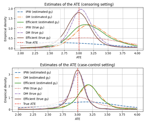
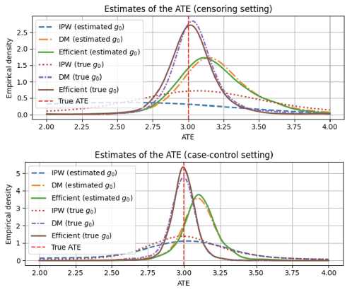
Figure 3: Empirical distributions of ATE estimates.

Figure 4: Empirical distributions of ATE estimates.

Appendix H Additional results of the simulation studies

This section investigates the case where the expected outcomes and propensity scores follow non-linear models.

All experiments were conducted on a Mac computer equipped with an Apple M2 processor and 24 GB of RAM.

H.1 Censoring setting

We generate synthetic data under the censoring setting, where the covariates $X$ are drawn from a multivariate normal distribution as $X\sim\zeta(x)$, where $\zeta(x)$ is the density of $\mathcal{N}(0,I_{p})$, $p$ represents the number of covariates and $I_{p}$ denotes the $(p\times p)$ identity matrix. For dimension, we set $p=10$. The propensity score is $g_{0}(1\mid X)=\mathrm{sigmoid}(X^{\top}\beta_{1}+X^{2\top}\beta_{2})$, where $X^{2}$ is the vector whose each element is the square of the corresponding element of vector $X$, $\beta_{1}$ and $\beta_{2}$ are coefficient vectors sampled from $\mathcal{N}(0,0.5I_{2p})$, and $D$ is sampled from the propensity score. The observation indicator $O$ is generated as $O_{i}=1$ from a Bernoulli distribution with probability $c$ if $D_{i}=1$ and $O_{i}=0$ if $D_{i}=0$. Here, $c$ is generated from a uniform distribution with support $[0,1]$ in advance of the experiment. The outcome is generated as $Y=(X^{\top}\beta)^{2}+1.1+\tau_{0}\cdot D+\varepsilon$, where $\varepsilon\sim\mathcal{N}(0,1)$, where we set $\tau_{0}=3$.

The nuisance parameters are estimated using three-layer perceptrons whose hidden layer has $100$-nodes. The convergence rates satisfy Assumption 4.6 under regular conditions (Schmidt-Hieber, 2020). We compared our proposed estimator, $\widehat{\tau}^{\mathrm{cens}\mathchar 45\relax\mathrm{eff}}_{n}$, with the other candidates, the IPW estimator $\widehat{\tau}^{\mathrm{cens}\mathchar 45\relax\mathrm{IPW}}_{n}$ and the DM estimator $\widehat{\tau}^{\mathrm{cens}\mathchar 45\relax\mathrm{DM}}_{n}$, defined in Remarks Remark and Remark, respectively. Note that all of these estimators are proposed by us, and our goal is not to confirm $\widehat{\tau}^{\mathrm{cens}\mathchar 45\relax\mathrm{eff}}_{n}$ outperforms the others, while our recommendation is $\widehat{\tau}^{\mathrm{cens}\mathchar 45\relax\mathrm{eff}}_{n}$. We consider both cases where the propensity score is either estimated using the method proposed by Elkan & Noto (2008) or assumed to be known.

We set $n=3000$. We conduct $5000$ trials and report the empirical MSEs and biases for the true ATE and the coverage ratio computed from the confidence intervals in Table 3 for $n=3000$ and Table 3 for $n=500$. We also present the empirical distributions of the ATE estimates in Figure 4 for $n=3000$ and Figure 4 for $n=5000$.

H.2 Case-control setting

In the case-control setting, covariates for the treatment and unknown groups are generated from $p=3$-dimensional different normal distributions: $X_{{\mathrm{T}}}\sim\zeta_{{\mathrm{T}},0}(x)$ and $X\sim\zeta_{0}(x)=e_{0}(1)\zeta_{{\mathrm{T}},0}(x)+e_{0}(0)\zeta_{{\mathrm{C}}}(x)$, where $\zeta_{{\mathrm{T}},0}(x)$ and $\zeta_{{\mathrm{C}}}(x)$ are the densities of normal distributions $\mathcal{N}(\mu_{p}\bm{1}_{p},I_{p})$ and $\mathcal{N}(\mu_{n}\bm{1}_{p},I_{p})$, $\mu_{p}=0.5$ and $\mu_{n}=0$, $\bm{1}_{p}=(1\ 1\ \cdots\ 1)^{\top}$, and $e(1)$ is the class prior set as $e(1)=0.3$. By definition, the propensity score $e_{0}(d\mid x)$ is given as $e_{0}(1\mid x)=e(1)\zeta_{{\mathrm{T}},0}(x)/\zeta_{0}(x)$. The outcome is generated similarly to the censoring setting $Y=(X^{\top}\beta)^{2}+1.1+\tau_{0}D+\varepsilon$, where $\tau_{0}=3$.

Since we use neural networks, We estimate the propensity score $g_{0}$ using the non-negative PU learning method proposed by Kiryo et al. (2017). Kiryo et al. (2017) introduces the non-negative PU learning method to mitigate the overfitting problem that arises when neural networks are used. For simplicity, we assume that the class prior $e_{0}(1)$ is known.

We consider two cases: $(m,l)=(1000,2000),(2000,3000)$. We conduct $5000$ trials and report the empirical MSEs and biases for the true ATE and the coverage ratio computed from the confidence intervals in Table 3 for $(m,l)=(1000,2000)$ and Table 3 for $(m,l)=(2000,3000)$. We also present the empirical distributions of the ATE estimates in Figure 4 for $(m,l)=(1000,2000)$ and Figure 4 for $(m,l)=(2000,3000)$.

References

- Ahn et al. (2011) Jaeil Ahn, Bhramar Mukherjee, Stephen B. Gruber, and Samiran Sinha. Missing exposure data in stereotype regression model: Application to matched case–control study with disease subclassification. Biometrics, 67(2):546–558, 2011.
- Bang & Robins (2005) Heejung Bang and James M. Robins. Doubly robust estimation in missing data and causal inference models. Biometrics, 61(4):962–973, 2005.
- Bekker & Davis (2018) Jessa Bekker and Jesse Davis. Learning from positive and unlabeled data under the selected at random assumption. In Proceedings of the Second International Workshop on Learning with Imbalanced Domains: Theory and Applications, volume 94, pp. 8–22, 2018.
- Bekker & Davis (2020) Jessa Bekker and Jesse Davis. Learning from positive and unlabeled data: a survey. Machine Learning, 109(4):719–760, 2020.
- Black et al. (2008) Sandra E. Black, Paul J. Devereux, and Kjell G. Salvanes. Staying in the classroom and out of the maternity ward? the effect of compulsory schooling laws on teenage births. The Economic Journal, 118(530):1025–1054, 2008.
- Chakrabortty & Dai (2024) Abhishek Chakrabortty and Guorong Dai. A general framework for treatment effect estimation in semi-supervised and high dimensional settings, 2024. arXiv:2201.00468.
- Chernozhukov et al. (2018) Victor Chernozhukov, Denis Chetverikov, Mert Demirer, Esther Duflo, Christian Hansen, Whitney Newey, and James Robins. Double/debiased machine learning for treatment and structural parameters. The Econometrics Journal, 2018.
- du Plessis & Sugiyama (2014) M. C. du Plessis and M. Sugiyama. Class prior estimation from positive and unlabeled data. IEICE Transactions on Information and Systems, E97-D(5):1358–1362, 2014.
- du Plessis et al. (2015) Marthinus Christoffel du Plessis, Gang. Niu, and Masashi Sugiyama. Convex formulation for learning from positive and unlabeled data. In International Conference on Machine Learning (ICML), pp. 1386–1394, 2015.
- Elkan & Noto (2008) Charles Elkan and Keith Noto. Learning classifiers from only positive and unlabeled data. In International Conference on Knowledge Discovery and Data Mining (KDD), pp. 213–220. Association for Computing Machinery, 2008.
- Hahn (1998) Jinyong Hahn. On the role of the propensity score in efficient semiparametric estimation of average treatment effects. Econometrica, 66(2):315–331, 1998.
- Hausman (2001) Jerry Hausman. Mismeasured variables in econometric analysis: Problems from the right and problems from the left. Journal of Economic Perspectives, 15(4), 2001.
- Horvitz & Thompson (1952) Daniel G. Horvitz and Donovan J. Thompson. A generalization of sampling without replacement from a finite universe. Journal of the American Statistical Association, 47(260):663–685, 1952.
- Hsieh et al. (2019) Yu-Guan Hsieh, Gang Niu, and Masashi Sugiyama. Classification from positive, unlabeled and biased negative data. In International Conference on Machine Learning (ICML), volume 97, pp. 2820–2829, 2019.
- Imbens & Rubin (2015) Guido W. Imbens and Donald B. Rubin. Causal Inference for Statistics, Social, and Biomedical Sciences: An Introduction. Cambridge University Press, 2015.
- Imbens & Wooldridge (2009) Guido W. Imbens and Jeffrey M. Wooldridge. Recent developments in the econometrics of program evaluation. Journal of Economic Literature, 47(1):5–86, 2009.
- Kanamori et al. (2009) Takafumi Kanamori, Shohei Hido, and Masashi Sugiyama. A least-squares approach to direct importance estimation. Journal of Machine Learning Research, 10(48):1391–1445, 2009.
- Kato & Teshima (2021) Masahiro Kato and Takeshi Teshima. Non-negative bregman divergence minimization for deep direct density ratio estimation. In International Conference on Machine Learning (ICML), 2021.
- Kato et al. (2018) Masahiro Kato, Liyuan Xu, Gang Niu, and Masashi Sugiyama. Alternate estimation of a classifier and the class-prior from positive and unlabeled data, 2018. arXiv:1809.05710.
- Kato et al. (2019) Masahiro Kato, Takeshi Teshima, and Junya Honda. Learning from positive and unlabeled data with a selection bias. In International Conference on Learning Representations (ICLR), 2019.
- Kato et al. (2021) Masahiro Kato, Takuya Ishihara, Junya Honda, and Yusuke Narita. Efficient adaptive experimental design for average treatment effect estimation, 2021. arXiv:2002.05308.
- Kato et al. (2024) Masahiro Kato, Akihiro Oga, Wataru Komatsubara, and Ryo Inokuchi. Active adaptive experimental design for treatment effect estimation with covariate choice. In International Conference on Machine Learning (ICML), 2024.
- Kennedy (2020) Edward H. Kennedy. Efficient nonparametric causal inference with missing exposure information. The International Journal of Biostatistics, 16(1), 2020.
- Kiryo et al. (2017) Ryuichi Kiryo, Gang Niu, Marthinus Christoffel du Plessis, and Masashi Sugiyama. Positive-unlabeled learning with non-negative risk estimator. In Advances in Neural Information Processing Systems (NeurIPS), pp. 1675–1685, 2017.
- Klaassen (1987) Chris A. J. Klaassen. Consistent estimation of the influence function of locally asymptotically linear estimators. Annals of Statistics, 15, 1987.
- Kuzmanovic et al. (2023) Milan Kuzmanovic, Tobias Hatt, and Stefan Feuerriegel. Estimating conditional average treatment effects with missing treatment information. In International Conference on Artificial Intelligence and Statistics (AISTATS), 2023.
- Lancaster & Imbens (1996) Tony Lancaster and Guido Imbens. Case-control studies with contaminated controls. Journal of Econometrics, 71(1):145–160, 1996.
- Lewbel (2007) Arthur Lewbel. Estimation of average treatment effects with misclassification. Econometrica, 75(2):537–551, 2007.
- Mahajan (2006) Aprajit Mahajan. Identification and estimation of regression models with misclassification. Econometrica, 74(3):631–665, 2006.
- Manski (1993) Charles F. Manski. Identification problems in the social sciences. Sociological Methodology, 23:1–56, 1993.
- Manski (2010) Charles F. Manski. Partial Identification in Econometrics, pp. 178–188. Palgrave Macmillan UK, 2010.
- Molinari (2010) Francesca Molinari. Missing treatments. Journal of Business & Economic Statistics, 28(1):82–95, 2010.
- Neyman (1923) Jerzy Neyman. Sur les applications de la theorie des probabilites aux experiences agricoles: Essai des principes. Statistical Science, 5:463–472, 1923.
- Niu et al. (2016) Gang Niu, Marthinus Christoffel du Plessis, Tomoya Sakai, Yao Ma, and Masashi Sugiyama. Theoretical comparisons of positive-unlabeled learning against positive-negative learning. In Advances in Neural Information Processing Systems (NeurIPS), volume 29. Curran Associates, Inc., 2016.
- Qin (1998) Jing Qin. Inferences for case-control and semiparametric two-sample density ratio models. Biometrika, 85(3):619–630, 1998.
- Ramaswamy et al. (2016) Harish Ramaswamy, Clayton Scott, and Ambuj Tewari. Mixture proportion estimation via kernel embeddings of distributions. In International Conference on Machine Learning (ICML), pp. 2052–2060, 2016.
- Rubin (1974) Donald B. Rubin. Estimating causal effects of treatments in randomized and nonrandomized studies. Journal of Educational Psychology, 66:688–701, 1974.
- Schmidt-Hieber (2020) Johannes Schmidt-Hieber. Nonparametric regression using deep neural networks with ReLU activation function. The Annals of Statistics, 48(4), 2020.
- Schuler & van der Laan (2024) Alejandro Schuler and Mark van der Laan. Introduction to modern causal inference, 2024.
- Steinberg & Cardell (1992) Dan Steinberg and N. Scott Cardell. Estimating logistic regression models when the dependent variable has no variance. Communications in Statistics - Theory and Methods, 21(2):423–450, 1992.
- Sugiyama et al. (2008) Masashi Sugiyama, Taiji Suzuki, Shinichi Nakajima, Hisashi Kashima, Paul von Bünau, and Motoaki Kawanabe. Direct importance estimation for covariate shift adaptation. Annals of the Institute of Statistical Mathematics, 60(4):699–746, 2008.
- Sugiyama et al. (2012) Masashi Sugiyama, Taiji Suzuki, and Takafumi Kanamori. Density Ratio Estimation in Machine Learning. Cambridge University Press, 2012.
- Sugiyama et al. (2022) Masashi Sugiyama, Han Bao, Takashi Ishida, Nan Lu, and Tomoya Sakai. Machine Learning from Weak Supervision: An Empirical Risk Minimization Approach (Adaptive Computation and Machine Learning series). The MIT Press, 2022.
- Syrgkanis (2017) Vasilis Syrgkanis. A proof of orthogonal double machine learning with -estimators, 2017. arXiv:1704.03754.
- Uehara et al. (2020) Masatoshi Uehara, Masahiro Kato, and Shota Yasui. Off-policy evaluation and learning for external validity under a covariate shift. In Conference on Neural Information Processing Systems (NeurIPS), 2020.
- van der Vaart (1998) Aad W. van der Vaart. Asymptotic Statistics. Cambridge Series in Statistical and Probabilistic Mathematics. Cambridge University Press, 1998.
- Wooldridge (2001) Jeffrey M. Wooldridge. Asymptotic properties of weighted m-estimation for standard stratified samples. Econometric Theory, 2001.
- Yamane et al. (2018) Ikko Yamane, Florian Yger, Jamal Atif, and Masashi Sugiyama. Uplift modeling from separate labels. In International Conference on Neural Information Processing Systems (NeurIPS), 2018.
- Zhang et al. (2013) Zhiwei Zhang, Wei Liu, Bo Zhang, Li Tang, and Jun Zhang. Causal inference with missing exposure information: Methods and applications to an obstetric study. Statistical methods in medical research, 25, 12 2013.
- Zhao & Ding (2024) Anqi Zhao and Peng Ding. To adjust or not to adjust? estimating the average treatment effect in randomized experiments with missing covariates. Journal of the American Statistical Association, 119(545):450–460, 2024.