Covering Multiple Objectives with a Small Set of Solutions Using Bayesian Optimization

Abstract

In multi-objective black-box optimization, the goal is typically to find solutions that optimize a set of $T$ black-box objective functions, $f_{1},\ldots f_{T}$, simultaneously. Traditional approaches often seek a single Pareto-optimal set that balances trade-offs among all objectives. In this work, we introduce a novel problem setting that departs from this paradigm: finding a smaller set of $K$ solutions, where $K<T$, that collectively “covers” the $T$ objectives. A set of solutions is defined as “covering” if, for each objective $f_{1},\ldots f_{T}$, there is at least one good solution. A motivating example for this problem setting occurs in drug design. For example, we may have $T$ pathogens and aim to identify a set of $K<T$ antibiotics such that at least one antibiotic can be used to treat each pathogen. To address this problem, we propose Multi-Objective Coverage Bayesian Optimization (MOCOBO), a principled algorithm designed to efficiently find a covering set. We validate our approach through extensive experiments on challenging high-dimensional tasks, including applications in peptide and molecular design. Experiments demonstrate MOCOBO’s ability to find high-performing covering sets of solutions. Additionally, we show that the small sets of $K<T$ solutions found by MOCOBO can match or nearly match the performance of $T$ individually optimized solutions for the same objectives. Our results highlight MOCOBO’s potential to tackle complex multi-objective problems in domains where finding at least one high-performing solution for each objective is critical.

1 Introduction

Bayesian optimization (BO) (Jones et al., 1998; Shahriari et al., 2015; Garnett, 2023) is a general framework for sample-efficient optimiziation of black-box functions. By using a probabilistic surrogate model, such as a Gaussian process, Bayesian optimization balances exploration and exploitation to identify high-performing solutions with a limited number of function evaluations. BO has been successfully applied in a wide range of domains, including hyperparameter tuning (Snoek et al., 2012b; Turner et al., 2021), A/B testing (Letham et al., 2019), chemical engineering (Hernández-Lobato et al., 2017), drug discovery (Negoescu et al., 2011), and more.

In multi-objective optimization the typical assumption is that objectives inherently trade off with one another, motivating the search for Pareto-optimal solutions that balance these trade-offs. Multi-objective optimization methods focus on identifying diverse (in objective value) sets of solutions along the Pareto front to capture these trade-offs (Hernández-Lobato et al., 2015; Belakaria et al., 2019; Turchetta et al., 2019; Konakovic Lukovic et al., 2020; Daulton et al., 2021; Stanton et al., 2022; Belakaria et al., 2022). Indeed, without such trade-offs, optimization would trivialize into simply optimizing all of the objectives.

However, in many real-world scenarios, the trade-offs between objectives can become extreme, with some objectives being nearly mutually exclusive. This makes it virtually impossible to achieve satisfactory performance across all objectives simultaneously. Figure 1 provides a $1D$ example of this demonstrating how the Pareto-optimal points may fail to achieve acceptable performance on all objectives. Such scenarios motivate an interesting generalization of the multi-objective setting that arises in situations where we can propose a small set of solutions that together optimize the multiple objectives and avoid the implicit constraints imposed by extreme trade-offs.

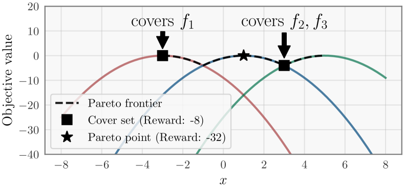
Figure 1: Traditional multi-objective optimization for $T$ objectives might select any point along the Pareto frontier, but in some situations like this any Pareto optimal point performs poorly on at least one objective. In situations where multiple $K<T$ solutions are allowed ($\blacksquare$), we can sometimes optimize all objectives well.

One compelling example arises in drug design. In this domain, the goal may be to develop antibiotics that treat a broad spectrum of pathogens–here, activity against the individual pathogens serve as the objectives. While it is very true that we seek to optimize the objectives simultaneously in the sense that we prefer to have broad-spectrum antibiotics, it is at the same time perfectly reasonable for one drug in the set to be ineffective against a few of the pathogens if it allows for greater potency against others. This flexibility enables a more targeted and efficient approach to therapeutic design, where our realistic goal is to have a small set of drugs that are together extremely lethal for the set of pathogens, without requiring each individual drug to be.

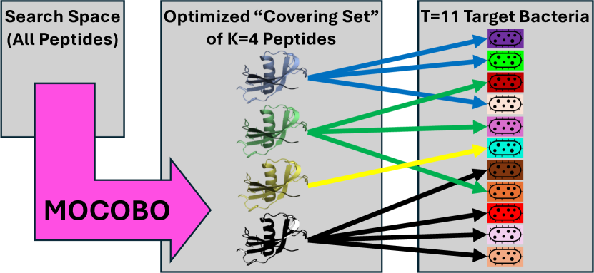
Figure 2: Diagram of example “coverage optimization” problem. MOCOBO seeks a set of $K=4$ peptides to cover $T=11$ target pathogenic bacteria. Arrows from peptides to bacteria indicate which peptides successfully inhibit (or “cover”) each bacteria in the target set. We provide results for this problem setting in Section 4.

To formalize this, we propose the “coverage optimization” problem: the task of covering a set of $T$ objectives with $K$ solutions, where coverage means that for each objective $f_{1},\dots,f_{T}$, there exists at least one high-performing solution among the $K$. In the context of drug design, this translates to identifying $K$ drugs such that each of the $T$ pathogens is effectively addressed by at least one drug in the set. This problem setting diverges from traditional multi-objective optimization by prioritizing collective coverage over balancing trade-offs within individual solutions. In Figure 2, we provide a diagram of one such “coverage optimization” problem considered in this paper.

To address this novel problem setting, we introduce and experimentally validate Multi-Objective Coverage Bayesian Optimization (MOCOBO), a new algorithm designed to solve the “coverage optimization” problem within the Bayesian optimization framework. MOCOBO efficiently identifies a small set of $K$ solutions that collectively cover $T$ objectives. Unlike traditional multi-objective methods that seek to balance trade-offs across all objectives for every solution, MOCOBO focuses on identifying specialized sets of solutions to meet practical coverage requirements.

Contributions

1. We introduce the problem setting of finding a “covering set” of $K<T$ high-performing solutions such that each relevant objective $f_{t}\in\left\{f_{1},\ldots f_{T}\right\}$ is optimized by at least one solution. This is the first work we are aware of to consider this problem setting.

2. We propose a local Bayesian optimization algorithm, MOCOBO, for this problem setting, that extends to high dimensional objectives, structured input domains, and large numbers of function evaluations.

3. We validate MOCOBO through experiments on challenging, high-dimensional optimization tasks including structured drug discovery over molecules and peptides, demonstrating its ability to consistently outperform state-of-the-art Bayesian optimization methods in identifying high-performing covering sets of solutions.

4. We provide empirical results demonstrating that the small sets $K<T$ solutions found by MOCOBO consistently nearly match the performance of a larger set of $T$ solutions individually optimized for each task.

5. We demonstrate the potential of MOCOBO for drug discovery using an in vitro experiment showing it produces potent antimicrobial peptides that cover 9/11 drug resistant or otherwise challenging to kill pathogens, with moderate activity on 1/11.

2 Background and Related Work

Bayesian optimization (BO).

BO (Močkus, 1975; Snoek et al., 2012a) is a methodology for sample-efficient black-box optimization. BO operates iteratively, where each cycle involves training a probabilistic surrogate model, typically a Gaussian process (GP) (Rasmussen, 2003), on data collected from the black-box objective function. BO then employs the predictive posterior $p(y\mid\mathbf{x},D)$ of the surrogate model to compute an acquisition function that gives a policy for determining the next candidate(s) to evaluate, balancing exploration and exploitation.

Multi-Objective Bayesian optimization (MOBO).

Recent advances in MOBO have introduced numerous methods aimed at identifying diverse solutions along the Pareto front to balance trade-offs among multiple objectives (Hernández-Lobato et al., 2015; Belakaria et al., 2019; Turchetta et al., 2019; Konakovic Lukovic et al., 2020; Daulton et al., 2021; Stanton et al., 2022; Belakaria et al., 2022). These approaches, however, are not well-suited to “coverage optimization”, where the goal is to find a small set of $K<T$ solutions that collectively address all $T$ objectives. Despite this, we compare our proposed method to MORBO, developed by Daulton et al. (2021), which is regarded as a state-of-the-art method for high-dimensional MOBO tasks.

Bayesian optimization over structured search spaces.

BO has recently been used for optimizing structured search spaces like molecules or amino acid sequences by employing latent space Bayesian optimization, which utilizes a variational autoencoder (VAE) to convert structured inputs into a continuous latent space for BO (Gómez-Bombarelli et al., 2018; Eissman et al., 2018; Tripp et al., 2020; Grosnit et al., 2021; Siivola et al., 2021; Jin et al., 2018; Stanton et al., 2022). The VAE encoder, $\Phi(\mathbf{x})$, transforms structured inputs $\mathbf{x}$ into continuous latent vectors $\mathbf{z}$, enabling BO to operate in the latent space. Candidate latent vectors are decoded using the VAE decoder, $\Gamma(\mathbf{z})$, to generate structured outputs. Maus et al. (2022) extended TuRBO (Eriksson et al., 2019) for latent space optimization by jointly training the surrogate model and VAE using variational inference.

Trust Region Bayesian Optimization (TuRBO).

Local Bayesian optimization (Eriksson et al., 2019), including TuRBO-$M$, is one recent successful approach to high-dimensional BO. TuRBO-$M$ uses $M$ parallel local optimization runs, each maintaining its own dataset $\mathcal{D}_{i}$ and surrogate model. Each local optimizer proposes candidates only within a hyper-rectangular trust region $\mathcal{T}_{i}$. The trust region $\mathcal{T}_{i}$ is a rectangular area of the input space $\mathcal{X}$, centered on the incumbent $\mathbf{x}^{+}_{i}$. Its side length $\ell_{i}$ is bound by $[\ell_{min},\ell_{max}]$. If an optimizer improves the incumbent for $\rho_{succ}$ consecutive iterations, $\ell_{i}$ expands to $\min(2\ell_{i},\ell_{max})$. If not improved in $\rho_{fail}$ iterations, $\ell_{i}$ is halved. Optimizers are restarted if $\ell_{i}$ drops below $\ell_{min}$. While TuRBO-$M$ is not directly applicable to our problem, we follow methods like MORBO (Daulton et al., 2021) and ROBOT (Maus et al., 2023) in adapting the use of $M$ coordinated trust regions ($K$ in our case) to a different problem setting.

3 Methods

We consider the task of finding a set of $K<T$ solutions $S^{*}=\left\{\mathbf{x}^{*}_{1},\ldots,\mathbf{x}^{*}_{K}\right\}$ that “covers” a set of $T$ objectives $f_{1},\ldots,f_{T}$. Here, the set $S^{*}$ “covers” the $T$ objectives if, for each objective $f_{t}=f_{1},\ldots,f_{T}$, there is at least one solution $\mathbf{x}^{*}_{k}\in S^{*}$ for which $f_{t}$ is well optimized by $\mathbf{x}^{*}_{k}$. We evaluate how well a set of $K$ points $\left\{\mathbf{x}_{1},\ldots,\mathbf{x}_{K}\right\}$ “covers” the $T$ objectives using following “coverage score” $c$:

$$c(\left\{\mathbf{x}_{1},\ldots,\mathbf{x}_{K}\right\}) =\sum_{t=1}^{T}\max_{k=1}^{K}f_{t}(\mathbf{x}_{k})$$ (1)

Formally, we seek a set $S^{*}:=\left\{\mathbf{x}^{*}_{1},\ldots,\mathbf{x}^{*}_{K}\right\}$ such that:

$$S^{*} =\operatorname*{arg\,max}_{\left\{\mathbf{x}_{1},\ldots,\mathbf{x}_{K}\right\}\subseteq\mathcal{X}}c(\left\{\mathbf{x}_{1},\ldots,\mathbf{x}_{K}\right\})$$ (2)

The coverage score in (1) only credits a single solution for each objective. If, for example, $f_{t}(\cdot)$ is maximized by one of the $\mathbf{x}_{i}$ in the solution set, improving the value of $f_{t}(\cdot)$ on some other $\mathbf{x}_{j\neq i}$ becomes irrelevant so long as $f_{t}(\mathbf{x}_{i})\geq f_{t}(\mathbf{x}_{j})$. In the setting where $K=1$, the coverage score collapses into a trivial linearization of the objectives and true multi-objective BO methods should be preferred. In the setting where $K=T$, the coverage score is trivially optimized by maximizing each objective independently.

3.1 Multi-Objective Coverage Bayesian Optimization (MOCOBO)

In this section, we propose MOCOBO - an algorithm which extends Bayesian optimization to the problem setting above.

In order to find a set of $K$ solutions, MOCOBO maintains $K$ simultaneous local optimization runs using $K$ individual trust regions. Each local run $k\in\left\{1,\ldots,K\right\}$ aims to find a single solution $\mathbf{x}^{*}_{k}$, which together form the desired set $S^{*}$. As in the original TuRBO paper, trust regions are rectangular regions of the search space $\mathcal{T}_{k}\subseteq\mathcal{X}$ defined solely by their size and center point.

On each step of optimization $s$, we use our current set of all data evaluated so far $D_{s}=\left\{(\mathbf{x}_{1},\mathbf{y}_{1}),\ldots,(\mathbf{x}_{n},\mathbf{y}_{n})\right\}$ to define the best covering set $S^{*}_{D_{s}}=\left\{\mathbf{x}^{*(s)}_{1},\ldots,\mathbf{x}^{*(s)}_{K}\in D_{s}\right\}$ found so far. Here $\mathbf{y}_{i}=(f_{1}(\mathbf{x}_{i}),\ldots,f_{T}(\mathbf{x}_{i}))$ and $n$ is the number of data points evaluated so far at step $s$. Following Equation 2, we define $S^{*}_{D_{s}}$ as follows:

$$S^{*}_{D_{s}} =\operatorname*{arg\,max}_{\left\{\mathbf{x}_{1},\ldots,\mathbf{x}_{K}\right\}\subseteq D_{s}}c(\left\{\mathbf{x}_{1},\ldots,\mathbf{x}_{K}\right\})$$ (3)

$$=\operatorname*{arg\,max}_{\left\{\mathbf{x}_{1},\ldots,\mathbf{x}_{K}\right\}\subseteq D_{s}}\sum_{t=1}^{T}\max_{k=1}^{K}f_{t}(\mathbf{x}_{k})$$ (4)

$c(S^{*}_{D_{s}})$ denotes the best coverage score found by the optimizer after optimization step $s$.

Since we select and evaluate $q$ candidates from each of the $K$ local optimization runs on each step of optimization, $n=s\times K\times q$.

3.1.1 Candidate Selection with Expected Coverage Improvement (ECI)

Given $S^{*}_{D_{s}}$, our surrogate model’s predictive posterior $p(y\mid\mathbf{x},D)$ induces a posterior belief about the improvement in coverage score achievable by choosing to evaluate at $\mathbf{x}$ next. We extend the typical expected improvement (EI) acquisiton function in the natural way to the coverage optimization setting by defining expected coverage improvement (ECI):

$$ECI(\mathbf{x}) =\mathbb{E}_{p(y|\mathbf{x},D)}[\max(0,c(S^{*}_{D_{s}\cup\left\{(\mathbf{x},\mathbf{y})\right\}})-c(S^{*}_{D_{s}}))]$$ (5)

Here $c(S^{*}_{D_{s}})$ is the coverage score of the best possible covering set from among all data observed $D_{s}$ – as we shall see, constructing this set $S^{*}_{D_{s}}$ will be our primary challenge. $c(S^{*}_{D_{s}\cup\left\{(\mathbf{x},\mathbf{y})\right\}})$ is the coverage score of the best possible covering set after adding the observation $(\mathbf{x},\mathbf{y})$. Thus, ECI gives the expected improvement in the coverage score after making an observation at point $\mathbf{x}$. We aim to select points during acquisition that maximize ECI.

We estimate ECI using a Monte Carlo (MC) approximation. To select a single candidate $\hat{\mathbf{x}}_{k}$ from $\mathcal{T}_{k}$, we sample $m$ points $P_{k}=\left\{\mathbf{p}_{k1},\mathbf{p}_{k2},...,\mathbf{p}_{km}\right\}$ from $\mathcal{T}_{k}$. For each sampled point $\mathbf{p}_{kj}$, we sample a realization $\hat{\mathbf{y}}_{kj}=(\hat{f}_{1}(\mathbf{p}_{kj}),\ldots,\hat{f}_{T}(\mathbf{p}_{kj}))$ from the GP surrogate model posterior. We leverage these samples to compute an MC approximation to the ECI of each $\mathbf{p}_{kj}$:

$$CI(\mathbf{p}_{kj}) =\max(0,c(S^{*}_{D_{s}\cup\left\{(\mathbf{p}_{kj},\hat{\mathbf{y}}_{kj})\right\}}-c(S^{*}_{D_{s}})))$$ (6)

Here, $c(S^{*}_{D_{s}\cup\left\{(\mathbf{p}_{kj},\hat{\mathbf{y}}_{kj})\right\}})$ is the approximation of the coverage score of the new best covering set if we choose to evaluate candidate $\mathbf{p}_{kj}$, assuming the candidate point will have the sampled objective values $\hat{\mathbf{y}}_{kj}$. We select and evaluate the candidate $\mathbf{p}_{kj}$ with largest expected coverage improvement.

3.1.2 Greedy Approximation of $S^{*}_{D_{s}}$

The candidate acquisition method in Section 3.1.1 utilizes the best covering set of $K$ points among all data collected so far, $S^{*}_{D_{s}}$. On each step of optimization $s$, MOCOBO must therefore construct $S^{*}_{D_{s}}$ from all observed data $D_{s}$, as $S^{*}_{D_{s}}$ may change on each step of optimization after new data is evaluated and added to $D_{s}$.

Lemma 3.1 (NP-hardness of Optimal Covering Set).

Let $T,K$ be finite positive integers such that $K<T$. Let $f_{1},\ldots,f_{T}$ be real valued functions. Let $D_{s}=\left\{(\mathbf{x}_{1},\mathbf{y}_{1}),\ldots,(\mathbf{x}_{n},\mathbf{y}_{n})\right\}$ be a dataset of $n$ real valued data points such that for all $\mathbf{x}_{i}$, $\mathbf{y}_{i}=(f_{1}(\mathbf{x}_{i}),\ldots,f_{T}(\mathbf{x}_{i}))$. Let $S^{*}_{D_{s}}$ be the optimal covering set of size $K$ in $D_{s}$ as defined in Equation 4. Then, constructing $S^{*}_{D_{s}}$ is NP-hard.

Proof.

See full proof of Lemma 3.1 in Section A.6. ∎

Since constructing $S^{*}_{D_{s}}$ is NP-hard, we use an approximate construction of $S^{*}_{D_{s}}$ on each step of optimization $s$. We present Algorithm 1 with $O(nKT)$ running time that achieves a constant $(1-\frac{1}{e})$ approximation factor.

Algorithm 1 Greedy $(1-\frac{1}{e})$-Approximation for Finding $S^{*}_{D_{s}}$ (Incremental Strategy)

0: Dataset $D_{s}$ with observed values $f_{t}(\mathbf{x})$ for all $t\in\{1,\ldots,T\}$ and $\mathbf{x}\in D_{s}$, covering set size $K$.

1: Initialize $A\leftarrow\emptyset$. {Start with an empty set.}

2: Compute the initial coverage score for $A$: $c(A)\leftarrow 0$.

3: for $k=1$ to $K$ do

4:  Initialize $\mathbf{x}_{\text{best}}\leftarrow\text{None}$ and $\Delta_{\text{best}}\leftarrow-\infty$.

5:  for $\mathbf{x}\in D_{s}\setminus A$ do

6:   Compute the marginal coverage of adding $\mathbf{x}$ to $A$:

$$\Delta c\leftarrow\sum_{t=1}^{T}\max\left(\max_{\mathbf{x}^{\prime}\in A}f_{t}(\mathbf{x}^{\prime}),f_{t}(\mathbf{x})\right)-c(A).$$

7:   if $\Delta c>\Delta_{\text{best}}$ then

8:    $\mathbf{x}_{\text{best}}\leftarrow\mathbf{x}$ and $\Delta_{\text{best}}\leftarrow\Delta c$.

9:   end if

10:  end for

11:  Update $A\leftarrow A\cup\{\mathbf{x}_{\text{best}}\}$, $c(A)\leftarrow c(A)+\Delta_{\text{best}}$.

12: end for

13: Output: $A^{*}_{D_{s}}\leftarrow A$.

Theorem 3.2 (Algorithm 1 provides a $(1-\frac{1}{e})$-Approximation of $S^{*}_{D_{s}}$).

Algorithm 1 provides a $(1-\frac{1}{e})$-Approximation of $S^{*}_{D_{s}}$. Formally, for the approximate covering set $A^{*}_{D_{s}}$ output by Algorithm 1:

$$c(A^{*}_{D_{s}})\geq\left(1-\frac{1}{e}\right)c(S^{*}_{D_{s}})$$

Proof.

See full proof of Theorem 3.2 in Section A.7. ∎

Algorithm 1 runtime.

The algorithm iterates $K$ times to construct the covering set. In each iteration, it evaluates at most $n$ candidate points, and for each candidate, it computes the incremental coverage score by iterating over $T$ objectives. The runtime is thus $O(K\cdot n\cdot T)$. For practical applications where we can assume relatively small $K$ and $T$, the runtime is approximately $O(n)$.

Corollary 3.3 (Algorithm 1 is the best possible approximation of $S^{*}_{D_{s}}$).

There is no polynomial runtime algorithm that provides a better approximation ratio unless $P=NP$.

Proof.

This follows from the fact that we reduced from Max $k$-cover, for which a better approximation ratio is not practically achievable unless $P=NP$ (Feige, 1998). ∎

3.1.3 MOCOBO Trust Region Dynamics

After each optimization step $s$, we center each trust region $\mathcal{T}_{k}$ on the corresponding point $\mathbf{x}^{*(s)}_{k}$ in the best observed covering set $S^{*}_{D_{s}}=\left\{\mathbf{x}^{*(s)}_{1},\ldots,\mathbf{x}^{*(s)}_{K}\right\}$ found so far, as defined in Equation 4. As in the original TuRBO algorithm, each trust region $\mathcal{T}_{k}$ has success and failure counters that dictate the size of the trust region. For MOCOBO, we count a success for trust region $\mathcal{T}_{k}$ whenever $\mathcal{T}_{k}$ proposes a candidate on step $s$ that improves upon the best coverage score and is included in $S^{*}_{D_{s+1}}$.

3.1.4 Extending ECI to the Batch Acquisition Setting (q-ECI)

In the batch acquisition setting, we select a batch of $q>1$ candidates for evaluation from each trust region. Following recent work on batch expected improvement (Wilson et al., 2017; Wang et al., 2019), we define q-ECI, a natural extension of ECI to the batch setting:

$$q\text{-ECI}(\mathbf{X})=\\ \mathbb{E}_{p(\mathbf{Y}|\mathbf{X},D)}\left[\max(0,\max_{r=1,\dots,q}c(S^{*}_{D_{s}\cup\left\{(\mathbf{x}_{r},\mathbf{y}_{r})\right\}})-c(S^{*}_{D_{s}}))\right]$$ (7)

q-ECI gives the expected improvement in the coverage score after simultaneously observing the batch of $q$ points $\mathbf{X}=\left\{\mathbf{x}_{1},\ldots,\mathbf{x}_{q}\right\}$. However, the resulting Monte Carlo expectation would require $O(q\times m)$ evaluations of Algorithm 1. We therefore adopt a more approximate batching strategy for practical use with large $q$ (see Section A.3 for a discussion of q-ECI intractability and our approximation).

4 Experiments

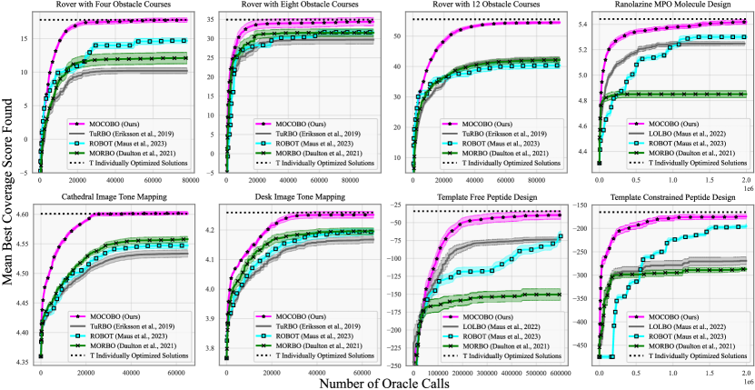
Figure 3: Coverage optimization results on all tasks considered.

We evaluate MOCOBO on four high-dimensional, multi-objective BO tasks for which finding a set of $K<T$ solutions to cover the $T$ objectives is desirable. Detailed descriptions of each task are in Section 4.2. Two tasks involve continuous search spaces, allowing direct application of MOCOBO, while the other two involve structured spaces (molecules and peptides), requiring an extension for structured optimization.

Implementation details and hyperparameters.

We implement MOCOBO using BoTorch (Balandat et al., 2020) and GPyTorch (Gardner et al., 2018). Code to reproduce all results in the paper will be made publicly available on github after the paper is accepted, with a link to the git repository provided here placeholder. We use an acquisition batch size of $20$ for all tasks and across all methods compared. Further implementation details are provided in subsection A.4. For our structured optimization problems, we apply MOCOBO in the latent space of a pre-trained VAE on which we perform regular end-to-end updates with the surrogate model during optimization (Maus et al., 2022).

Plots.

In Figure 3, we plot the best coverage score $c$ Equation 1 obtained by the $K$ best covering solutions found so far after a certain number of function evaluations on each task. Since baseline methods are not designed to optimize coverage directly, instead aiming to find a single solution or a set of solutions to optimize the $T$ objectives, we plot the best coverage score $c$ obtained by the $K$ best covering solutions found by the method. All plots show mean coverage scores averaged over $20$ replications of each method, and show standard errors.

4.1 Baselines

In all plots, we compare MOCOBO against TuRBO, ROBOT, and MORBO ((Eriksson et al., 2019; Maus et al., 2023; Daulton et al., 2021)). For each method, we compare to the performance of the best set of $K<T$ solutions found.

Extending baselines to the structured BO setting.

In the case of the two structured optimization tasks (molecule and peptide design), we apply LOL-BO and ROBOT as described by design for these problem settings. For MORBO, we take the straightforward approach of applying MORBO directly in the continuous latent space of the VAE model without other adaptations. The same pre-trained VAE model is used across methods compared.

Extending baselines to the coverage BO setting.

As TuRBO, LOL-BO, and ROBOT target single-objective optimization, we conduct $T$ independent runs to optimize each of the $T$ objectives for the multi-objective task. We use all solutions gathered from the $T$ runs to compute the best covering set of $K$ solutions found by each method.

Unlike LOL-BO and TuRBO which seek a single best solution for a given objective, a single run of ROBOT seeks a set of $M$ solutions that are pairwise diverse. We run ROBOT with $M=K$ so that each independent run of ROBOT seeks $M=K$ diverse solutions. The aggregate result of the $T$ independent runs for ROBOT is thus $K$ diverse solutions for each of the $T$ objectives. We compare to the best covering $K$ solutions from among those $K*T$ solutions. See Section A.4.4 for more details on diversity constraints used by ROBOT and the associated diversity hyperparameters used to run ROBOT on each task.

MORBO is a multi-objective optimization method and can thus be applied directly to each multi-objective optimization task. For each run of MORBO, we compare to the best covering set of $K$ solutions found among all solutions proposed by the run.

T individually optimized solutions baseline.

We also compare to a brute-force method involving $T$ separate single-objective optimizations for each of the $T$ objectives, using TuRBO for each run or LOL-BO for molecule and peptide design. This is not an alternative for finding $K<T$ covering solutions, but instead identifies $T$ solutions, one per objective, approximating a ceiling we can achieve on performance without the limit of $K<T$ solutions. Approaching the performance of this baseline implies that we can find $K$ solutions that do nearly as well as if we were allowed $T$ solutions instead.

4.2 Tasks

Peptide design.

In the peptide design task, we explore amino acid sequences to minimize the MIC (minimum inhibitory concentration, measured in $\mu$ mol $\text{L}^{-1}$) for each of $T=11$ target drug resistant strains or otherwise challenging to kill bacteria (B1-B7 Gram negative, B8-B11 Gram positive). Table A.5 lists our target bacteria in this study. Briefly, MIC indicates the concentration of peptide needed to inhibit bacterial growth (see Kowalska-Krochmal & Dudek-Wicher (2021)). We evaluate MIC for a given peptide sequence and bacteria using the APEX 1.1 model proposed by Wan et al. (2024). To frame the problem as maximization, we optimize $-\text{MIC}$. We seek $K=4$ peptides that together form a potent set of antibiotics for all $T=11$ bacteria. To enable optimization over peptides, we use the VAE model pre-trained on $4.5$ million amino acid sequences from Torres et al. (2024) to map the peptide sequence search space to a continuous $256$ dimensional space.

Template free vs template constrained peptide design.

We evaluate MOCOBO on two variations of the peptide design task: “template free” (TF) and “template constrained” (TC). For TF, we allow the optimizer to propose any sequence of amino acids. For TC, we add a constraint that any sequence proposed by the optimizer must have a minimum of $75$ percent sequence similarity to at least one of the $10$ template amino acid sequences in Table A.6. These $10$ templates were mined from extinct organisms and selected by Wan et al. (2024). The motivation of the template constrained task is to design peptides specifically likely to evade antibiotic resistance by producing “extinct-like” peptides that bacteria have not encountered in nature in thousands of years. We handle the optimization constraint by adapting techniques from SCBO (Eriksson & Poloczek, 2021).

Ranolazine MPO molecule design.

Ranolazine is a drug used to treat chest pain. The original Ranolazine MPO task from the Guacamol benchmark suite of molecular design tasks (Brown et al., 2019) aims to design an alternative to this drug: a molecule with a high fingerprint similarity to Ranolaize that includes fluorine. We extend this task to the multi-objective optimization setting by searching for alternatives to Ranolazine that include $T=6$ reactive nonmetal elements not found in Ranolazine: fluorine, chlorine, bromine, selenium, sulfur, and phosphorus. We aim to cover the $T=6$ objectives with $K=3$ molecules. We use the SELFIES-VAE introduced by Maus et al. (2022) to map the molecular space to a continuous $256$ dimensional space.

Rover.

The rover trajectory optimization task introduced by Wang et al. (2018) consists of finding a $60$-dimensional policy that allows a rover to move along some trajectory while avoiding a fixed set of obstacles. To frame this as a multi-objective optimization task, we design $T$ unique obstacle courses for the rover to navigate. The obstacle courses are designed such that no single policy can successfully navigate all courses. We seek $K<T$ policies so that at least one policy enables the rover to avoid obstacles in each course. We evaluate on three unique instances with varying numbers of obstacle courses. For the instances of this task with $T=4$ and $T=8$, we seek to cover the objectives with $K=2$ solutions. For the $T=12$ instance, we seek to cover the objectives with $K=4$ solutions.

Image tone mapping.

In high dynamic range (HDR) images, some pixels (often associated with light sources) can dominate overall contrast, requiring adjustments to reveal detail in low-contrast areas, a problem known as tone mapping (Reinhard et al., 2005, Section 6). Tone mapping algorithms involve various tunable parameters, resulting in a high-dimensional optimization problem of subjectively perceived quality. Because commonly used metrics are only correlated with subjective quality, tuning such parameters has been done by trial and error and human-in-the-loop type schemes (Lischinski et al., 2006), including preferential BO-based approaches (Koyama et al., 2017, 2020).

We seek a covering set of $K=4$ solutions to optimize a set of $T=7$ image aesthetic (IAA) and quality (IQA) assessment metrics from the pyiqa library (Chen & Mo, 2022) (see metrics listed in Table A.3). Our practical goal is that, while we do not know a priori which metric is best for a particular image, covering all metrics may result in at least one high quality image. We use the “Stanford Memorial Church” Debevec & Malik (1997) and “desk lamp” Čadík (2008) benchmark images. We optimize over the $13$-dimensional parameter space of an established tone mapping pipeline. See Section A.5.1 for details.

4.3 Optimization Results

In Figure 3, we provide optimization results comparing MOCOBO to the baselines discussed above on all tasks. The results show that MOCOBO finds sets of $K$ solutions that achieve higher coverage scores across tasks.

The “T Individually Optimized Solutions” baseline appears as a horizontal dotted line in all plots of Figure 3, representing the average coverage score of $T$ individually optimized solutions, serving as an approximation of the best possible performance without the constraint of a limited $K<T$ solution set. Results in Figure 3 demonstrate that the smaller set of $K<T$ solutions identified by MOCOBO nearly equals the performance of the complete set of $T$ individually optimized solutions. This result depends on using domain knowledge to choose $K$ large enough to achieve it. Results in Figure 3 show that matching the performance of $T$ optimized solutions is possible with some values of $K\ll T$.

Peptide Amino Acid Sequence	B1(-)	B2(-)	B3(-)	B4(-)	B5(-)	B6(-)	B7(-)	B8(+)	B9(+)	B10(+)	B11(+)
KKKKLKLKKLKKLLKLLKRL	1.017	1.040	1.893	0.999	8.613	0.966	1.039	65.999	38.361	338.692	1.393
IFHLKILIKILRLL	0.999	15.565	1.860	1.952	404.254	486.860	406.034	1.233	1.318	7.359	0.981
SKKIKLLGLALKLLKLKLKL	2.654	3.268	3.113	4.854	4.923	12.967	14.610	22.631	29.685	254.306	3.947
KKKKLKLKKLKRLLKLKLRL	0.939	0.906	1.124	1.310	10.909	1.384	1.711	12.776	32.884	434.193	1.037

Table 1: Best set of $K=4$ peptides found by one run of MOCOBO for the “template free” peptide design task. We provide the APEX model’s predicted MIC for each sequence on each of the $11$ target pathogenic bacteria. The target pathogenic bacteria B1$,\ldots,$ B11 are listed in Table A.5. (-) and (+) indicate Gram negative and Gram positive pathogenic bacteria respectively. The best/lowest MIC achieved for each pathogenic bacteria is in bold in each column. See row “TF1” in Figure 4 and Figure A.1 for in vitro MICs for this set of $K=4$ peptides. See Table A.1 for an analogous result on the “template constrained” peptide design task.

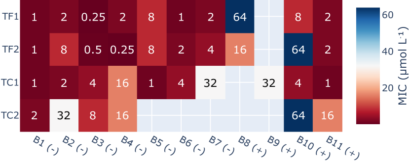
Figure 4: In vitro results for the two best “template free” (TF1, TF2) and two best “template constrained” (TC1, TC2) runs of MOCOBO for the peptide design task. Columns are the best/lowest in vitro MIC among the $K=4$ peptides found by MOCOBO for each target pathogenic bacteria B1$,\ldots,$ B11 listed in Table A.5. (-) and (+) indicate Gram negative and Gram positive respectively. TF1 and TC1 correspond to the single runs of MOCOBO shown in Table 1 and Table A.1 respectively. Methods used to obtain in vitro MICs are provided in Section A.1.

Figure 5: (Four Leftmost Panels) $T=4$ varied obstacle courses as multiple objectives for the rover task and $K=2$ covering trajectories (blue, magenta) found by MOCOBO. The first trajectory (magenta) successfully navigates obstacle courses 2 and 3 (second and third panels from the left). The second trajectory (blue) navigates obstacle courses 1 and 4 (first and fourth panels from the left). (Middle Panel) Initial hdr desk image for the desk variation of the “image tone mapping” task. (Four Rightmost Panels) Images obtained by transforming the hdr desk image using the best covering set of $K=4$ solutions found by a single run of MOCOBO.

Peptide design results.

In Table 1, we provide the $K=4$ peptides found by one run of MOCOBO for the “template free” peptide design task. For each of the four peptides, we provide the APEX model’s predicted MIC for each of the $11$ target bacteria. MIC values $\leq 16$ $\mu$ mol $L^{-1}$ are considered to be “highly active” against the target pathogenic bacteria (Wan et al., 2024). We highlight in Table 1 the comparison between the second peptide with the other three peptides. B1-B7 are Gram negative bacteria, while B8-B11 are Gram positive. Peptide 2 specialized to the Gram positive bacteria (B8-B11 scores predicted highly active compared to the other peptides) at the expense of broad spectrum activity for Gram negatives (B5, B6, B7 predictied inactive). By specializing its solutions to Gram negative and Gram positive bacteria separately, MOCOBO achieves low MIC across the target bacteria with only $K=4$ peptides. A similar table of results is also provided for the template constrained peptide design task (see Table A.1).

In Figure 4, we provide in vitro results for the two best “template free” and two best “template constrained” runs of MOCOBO for the peptide design task. Here, “best” means runs that achieved highest coverage scores according to the APEX 1.1 model. For each run, Figure 4 provides the best/lowest in vitro MIC among the $K=4$ peptides found by MOCOBO for each target pathogenic bacteria. Results demonstrate that solutions found by MOCOBO optimizing against the in-silico APEX 1.1 model achieve good coverage of the $11$ target pathogenic bacteria in vitro. In Figure A.1, we provide the full set of in vitro results for each these runs of MOCOBO, with MIC values obtained by each of the $K=4$ peptides found for each target bacteria. Methods used to obtain in vitro MICs are provided in Section A.1.

Molecule design results.

In Table A.2, we provide results for the $K=3$ molecules found by one run of MOCOBO for the molecule design task. Each of the $6$ target elements is successfully present in one of the $K=3$ molecules in the best covering set. These three molecules therefore effectively cover the $T=6$ objectives, with each objective having a max score $>0.9$.

Rover results.

In the four leftmost panels of Figure 5, we depict the $T=4$ obstacle courses that the rover seeks to navigate with a covering set of $K=2$ optimized trajectories (magenta, blue). Together, the two optimized trajectories cover the $T=4$ obstacle courses such that all obstacles are avoided. In Figure A.3 and A.4, we provide analogous figures for the $T=8$ and $T=12$ variations of the rover task. In each example, the MOCOBO optimized set of trajectories covers all obstacle courses such that all obstacles are avoided.

Image tone mapping results.

In the Figure 5 (five rightmost panels) and Figure A.2, we provide the original hdr images and the images obtained by the $K=4$ solutions found by a single run of MOCOBO for the church and desk test images respectively. In both variations, three of the four solutions result in high-quality images, while one solution results in a poor quality image (see middle right church image in Figure A.2 and rightmost desk image in Figure 5). The two poor quality images were both generated by the one solution in the best covering set that MOCOBO used to cover metrics $5$ and $6$ (see metric ID numbers in Table A.3). This indicates that metrics $5$ and $6$ are poor indicators of true image quality in this setting. Overall, this result highlights a useful application of MOCOBO: By dedicating one of the $K$ solutions to maximizing the misleading metrics ($5$ and $6$), the other $3$ solutions to can focus on the remaining subjectively better quality metrics.

A notable apparent limitation of the existing IAA/IQA metrics we used here is that they all favored monochromatic images for both the church and desk images. As such, the tone-mapped images obtained appear less colorful than their hand-tuned counterparts reported in prior work.

4.4 Ablation Study

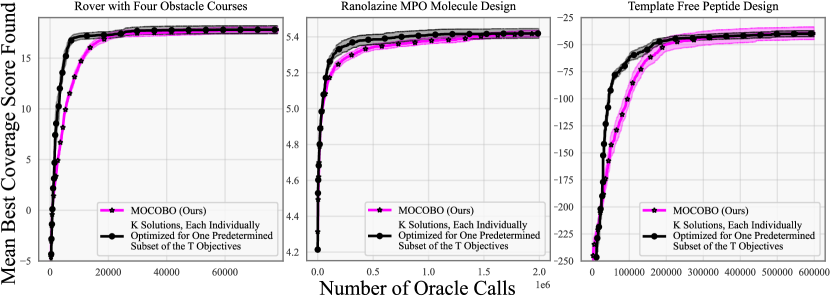
Figure 6: Ablation study comparing MOCOBO to optimization performance where a known “good” partitioning of the $T$ objectives into $K$ subsets is available in advance. We individually optimize $K$ solutions, one for each partition.

A challenging aspect of our problem setting is that we do not know a priori the best way(s) to divide the $T$ objectives into $K$ subsets such that good coverage can be obtained. In this section, we seek to answer the question: what is the efficiency lost by MOCOBO due to not knowing an efficient partitioning of the objectives in advance?. To construct a proxy “efficient” partition to measure this, we first run MOCOBO to completion on a task, and then consider optimization as if we had known the partitioning of objectives found at the end in advance.

With such an “oracle” partitioning in hand ahead of time, we can efficiently optimize by running $K$ independent optimization runs: one to find a single solution for each subset in the fixed, given partition. With a fixed partition, the coverage score in (1) reduces to optimizing the sum of objectives in each relevant subset independently.

In Figure 6 we compare this strategy directly to MOCOBO on three optimization tasks. We plot the best coverage score obtained by $K$ independent runs of TuRBO/LOL-BO on the fixed oracle $K$-partitioning of the objectives by combining their solutions into a single set. MOCOBO achieves the same average best coverage scores with minimal loss in optimization efficiency despite having to discover an efficient partitioning during optimization.

5 Discussion

By bridging the gap between traditional multi-objective optimization and practical coverage requirements, MOCOBO offers an effective approach to tackle critical problems in drug design and beyond. This framework extends the reach of Bayesian optimization into new domains, providing a robust solution to the challenges posed by extreme trade-offs and the need for specialized, collaborative solutions.

Impact Statement

This research includes applications in molecule and peptide design. While AI-driven biological design holds great promise for benefiting society, it is crucial to acknowledge its dual-use potential. Specifically, AI techniques designed for drug discovery could be misused to create harmful biological agents (Urbina et al., 2020).

Our goal is to accelerate drug development by identifying promising candidates, but it is imperative that experts maintain oversight, that all potential therapeutics undergo thorough testing and clinical trials, and that strict regulatory frameworks governing drug development and approval are followed.

Appendix A Appendix

A.1 Methods for Obtaining In Vitro Minimal Inhibitory Concentration (MIC) Data

In this section, we provide the methods used to produce all in vitro minimal inhibitory concentration (MIC) values reported in this paper.

Peptide synthesis.

All peptides were synthesized by solid-phase peptide synthesis using the Fmoc strategy and purchased from AAPPTec.

Bacterial strains and growth conditions used in the experiments.

The following Gram-negative bacteria were used in our study: Acinetobacter baumannii ATCC 19606, Escherichia coli ATCC 11775, E. coli AIC221 (E. coli MG1655 phn$E_{2}$::FRT), E. coli AIC222 (E. coli MG1655 pmrA53 phn$E_{2}$::FRT (colistin resistant)), Klebsiella pneumoniae ATCC 13883, Pseudomonas aeruginosa PAO1, and P. aeruginosa PA14. The following Gram-positive bacteria were also used in our study: Staphylococcus aureus ATCC 12600, S. aureus ATCC BAA-1556 (methicillin-resistant strain), Enetrococcus faecalis ATCC 700802 (vancomycin-resistant strain) and E. faecium ATCC 700221 (vancomycin-resistant strain). Bacteria were grown from frozen stocks and plated on Luria-Bertani (LB) or Pseudomonas isolation agar plates (P. aeruginosa strains) and incubated overnight at $37$ degrees Celsius. After the incubation period, a single colony was transferred to $6mL$ of LB medium, and cultures were incubated overnight ($16h$) at $37$ degrees Celsius. The following day, an inoculum was prepared by diluting the overnight cultures $1:100$ in $6ml$ of the respective media and incubating them at $37$ degrees Celsius until bacteria reached logarithmic phase ($OD_{600}=0.3-0.5$).

Antibacterial assays.

The in vitro antimicrobial activity of the peptides was assessed by using the broth microdilution assay (Cesaro et al., 2022). Minimal inhibitory concentration (MIC) values of the peptides were determined with an initial inoculum of $2\times 10^{6}$ cells $mL^{-1}$ in LB in microtiter $96$-well flat-bottom transparent plates. Aqueous solutions of the peptides were added to the plate at concentrations ranging from $0.0625$ to $64$ $\mu molL^{-1}$. The lowest concentration of peptide that inhibited 100 percent of the visible growth of bacteria was established as the MIC value in an experiment of $20h$ of exposure at 37 degrees Celsius. The optical density of the plates was measured at $600nm$ using a spectrophotometer. All assays were done as three biological replicates.

A.2 Additional Results

In this section, we provide additional examples of covering sets of solutions found by MOCOBO for various tasks from Section 4.

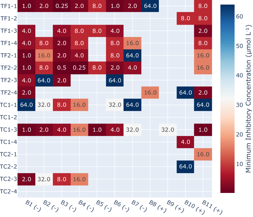
Figure A.1: In vitro results for the two best “template free” (TF1, TF2) and two best “template constrained” (TC1, TC2) runs of MOCOBO for the peptide design task. Here, “best” means runs that achieved highest coverage scores according to the APEX 1.1 model. Each row is a single peptide found by a run of MOCOBO. Row TF$i$-$j$ indicates template free run $i$, peptide $j$. Similarly, TC$i$-$j$ indicates template constrained run $i$, peptide $j$. Columns are the in vitro MICs for each target pathogenic bacteria B1$,\ldots,$ B11 listed in Table A.5. (-) and (+) indicate Gram negative and Gram positive respectively. TF1 and TC1 correspond to the single runs of MOCOBO shown in Table 1 and Table A.1 respectively. Methods used to obtain in vitro MICs are provided in Section A.1.

In Figure A.1, we provide In vitro results for the two best “template free” and two best “template constrained” runs of MOCOBO for the peptide design task. Here, “best” means runs that achieved highest coverage scores according to the APEX 1.1 model. Figure A.1 provides in vitro MICs for each of the $K=4$ peptides found by each of these runs of MOCOBO, for each of the $11$ target pathogenic bacteria. Methods used to obtain in vitro MICs are provided in Section A.1.

Peptide Amino Acid Sequence	B1(-)	B2(-)	B3(-)	B4(-)	B5(-)	B6(-)	B7(-)	B8(+)	B9(+)	B10(+)	B11(+)
KKLKIIRLLFK	18.594	17.067	4.278	5.352	13.460	50.442	24.543	456.831	431.276	441.292	20.305
WAIRGLKLATWLSLNNKF	6.771	20.358	14.644	10.477	65.172	97.404	59.195	19.846	33.459	237.697	7.708
RWARNLVRYVKWLKKLKKVI	2.171	4.589	2.641	3.073	54.400	11.444	19.150	75.588	89.977	413.386	2.913
HWITIAFFRLSISLKI	225.260	346.589	56.583	58.253	458.963	475.616	538.352	293.852	338.047	34.230	22.153

Table A.1: The best set of $K=4$ peptide sequences found by one run of MOCOBO for the “template free” peptide design task described in Section 4.2. For each of the four sequences, we provide the MIC according to the APEX model for each of the $11$ target pathogenic bacteria. The target pathogenic bacteria B1$,\ldots,$ B11 are listed in Table A.5. (-) and (+) indicate Gram negative and Gram positive pathogenic bacteria respectively. The best/lowest MIC achieved for each pathogenic bacteria is in bold in each column. See row “TC1” in Figure 4 and Figure A.1 for in vitro MICs for this set of $K=4$ peptides.

In Table A.1, we provide an example of a covering set of peptides found by MOCOBO for the “template constrained” variation of the peptide design task.

In Figure A.2, we provide the original hdr image (leftmost panel), and the $K=4$ images produced using the $K=4$ solutions found by a single run of MOCOBO for the church image variation of the image tone mapping task.

In Table A.2, we provide an example of a covering set of $K=3$ molecules found by MOCOBO for the molecule design task. As mentioned in Section 4, these three molecules effectively cover the $T=6$ objectives, as evidenced by the presence of all $T=6$ target elements in one of the $K=3$ molecules designed by MOCOBO.

In Figure A.3 and Figure A.4, we provide examples of a covering set of trajectories found for the $T=8$ and $T=12$ variations of the rover task respectively. In each figure, a panel is shown for each of the $T$ obstacles courses, with obstacles colored in red. The required starting point for the rover is a green point in the bottom left of each panel. The “goal” end point that the rover aims to reach without hitting any obstacles is the red point in the top right of each panel. Each panel also shows the best among the $K$ trajectories found by a run of MOCOBO for navigating each obstacle course. An analogous plot for the $T=4$ variation of the rover optimization task is provided in the main text in Figure 5.

Figure A.2: (Leftmost Panel) Initial hdr church image for the church test image variation of the “image tone mapping” task. (Four Rightmost Panels) Images obtained by transforming the hdr church image using the best covering set of $K=4$ solutions found by a single run of MOCOBO.

Molecule (Smiles String)	Obj 1 (add F)	Obj 2 (add Cl)	Obj 2 (add Br)	Obj 2 (add Se)	Obj 2 (add S)	Obj 2 (add P)
CC=C(C)C(OC(=O)C(O)CCCCCCC(=O)O)
=CC=CCCCCCC[Se]CC(=O)NC1=CC=CC=C1C	0.8038	0.8038	0.8038	0.9108	0.8038	0.8038
CC=C(C)C(OC(=O)CCCCCCC(O)C(=S)Cl)
=CC=CCOCCCCC(O)CC(=O)NC1=CC=CC=C1C	0.8043	0.9114	0.8043	0.8043	0.9114	0.8043
CC=C(C)C(OC(=O)C(O)CCCCCCC(=O)CBr)
=CC=COCPCCCCN(C)CC(=O)[NH1]C1=CC=C(F)C=C1C	0.9097	0.8028	0.9097	0.8028	0.8028	0.9097

Table A.2: The best set of $K=3$ molecules found by one run of MOCOBO for the Ranolazine MPO multiple element molecule design task described in Section 4.2. For each of the three molecules, we provide the objective value obtained for each of the $T=6$ objectives. The best/highest objective value is in bold in each column. Each objective aims to add a different target element to Ranolazine (F, Cl, Br, Se, S, and P). The $T=6$ target elements are in bold in the smiles string (Weininger, 1988) representation of each molecule.

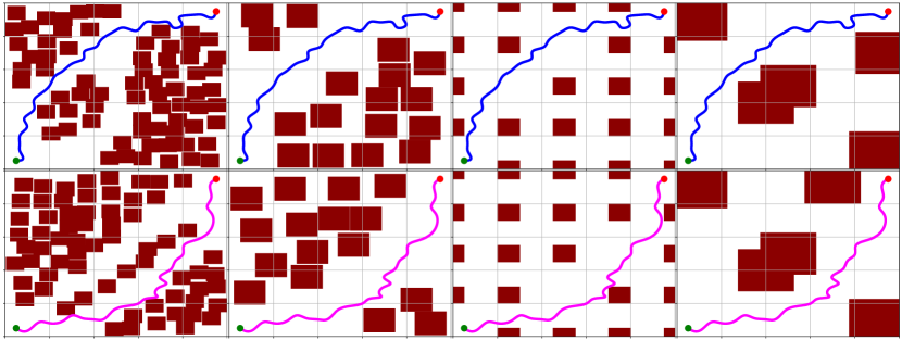
Figure A.3: The 8 panels depict the 8 obstacle courses that the rover must navigate for the $T=8$ variation of the rover task, with obstacles colored in red. The required starting point for the rover is a green point in the bottom left of each panel. The “goal” end point that the rover aims to reach without hitting any obstacles is the red point in the top right of each panel. The line in each panel shows the best trajectory for navigating the obstacle course from among the $K=2$ covering trajectories found by a single run of MOCOBO. The first trajectory in the covering set is shown in magenta and successfully navigates obstacle courses 5, 6, 7, and 8 (Bottom Row). The second is shown in blue and successfully navigates obstacle courses 1, 2, 3, and 4 (Top Row).

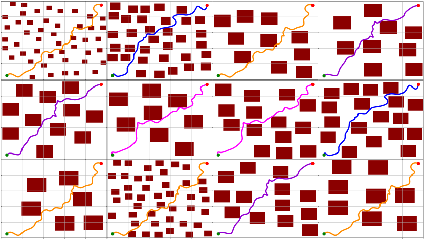
Figure A.4: The 12 panels depict the 12 obstacle courses that the rover must navigate for the $T=12$ variation of the rover task, with obstacles colored in red. The required starting point for the rover is a green point in the bottom left of each panel. The “goal” end point that the rover aims to reach without hitting any obstacles is the red point in the top right of each panel. The line in each panel shows the best trajectory for navigating each obstacle course from among the $K=4$ covering trajectories found by a run of MOCOBO. The first trajectory in the covering set is shown in magenta and successfully navigates obstacle courses 6 and 7 (Middle Row: Center Left and Center Right Panels). The second is shown in blue and successfully navigates obstacle courses 2 and 8 (Top Row: Center Left Panel, Middle Row: Rightmost Panel). The third is shown in purple and successfully navigates obstacle courses 4, 5, and 11 (Top Row: Rightmost Panel, Middle Row: Leftmost Panel, and Bottom Row: Center Right Panel). The fourth trajectory is shown in orange and successfully navigates obstacle courses 1, 3, 9, 10, and 12 (Top Row: Leftmost Panel and Center Right Panel, Bottom Row: Leftmost, Center Left, and Rightmost Panels).

A.3 Approximation Strategy for Batch Acquisition with Expected Coverage Improvement (ECI)

In batch acquisition, we select a batch of $q>1$ candidates from each trust region for evaluation. In Equation 7, we define q-ECI, a natural extension of the ECI acquisition function defined in Equation 5 to the batch acquisition setting. q-ECI gives the expected improvement in the coverage score after simultaneously observing the batch of $q$ points $\mathbf{X}=\left\{\mathbf{x}_{1},\ldots,\mathbf{x}_{q}\right\}$. When using batch acquisition, we aim to select a batch of $q$ points that maximize q-ECI.

We will first discuss how one would estimate q-ECI using a Monte Carlo (MC) approximation. To select a batch candidates $\hat{\mathbf{X}}_{k}$ from $\mathcal{T}_{k}$, we sample $m$ batches of $q$ points $B_{k}=\left\{\mathbf{B}_{k1},\mathbf{B}_{k2},...,\mathbf{B}_{km}\right\}$ from $\mathcal{T}_{k}$. Here $\mathbf{B}_{kj}$ is a batch of $q$ sampled points $\mathbf{B}_{kj}=\left\{\mathbf{b}_{kj1},\ldots,\mathbf{b}_{kjq}\right\}$. For each batch $\mathbf{B}_{kj}$, we sample a realization $\hat{\mathbf{Y}}_{kj}=\left\{\hat{\mathbf{y}}_{kj1},\ldots,\hat{\mathbf{y}}_{kjq}\right\}$ from the GP surrogate model posterior. We leverage these samples to compute an MC approximation to the q-ECI of each $\mathbf{B}_{kj}$:

$$q\text{-CI}(\mathbf{B}_{kj}) =\max(0,\max_{r=1,\dots,q}c(S^{*}_{D_{s}\cup\left\{(\mathbf{b}_{kjr},\hat{\mathbf{y}}_{kjr})\right\}})-c(S^{*}_{D_{s}}))$$ (8)

Here, $c(S^{*}_{D_{s}\cup\left\{(\mathbf{b}_{kjr},\hat{\mathbf{y}}_{kjr})\right\}})$ is the approximation of the coverage score of the new best covering set if we choose to evaluate candidate $\mathbf{b}_{kjr}$, assuming the candidate point will have the sampled objective values $\hat{\mathbf{y}}_{kjr}$. We would like to select and evaluate the batch of candidates $\mathbf{B}_{kj}$ with the largest $q\text{-CI}$.

Evaluating $q\text{-CI}$ for a single candidate batch requires $q$ evaluations of $c(S^{*}_{D_{s}\cup\left\{(\mathbf{b}_{kjr},\hat{\mathbf{y}}_{kjr})\right\}})$. Each evaluation of $c(S^{*}_{D_{s}\cup\left\{(\mathbf{b}_{kjr},\hat{\mathbf{y}}_{kjr})\right\}})$ requires a call to Algorithm 1 to first construct $S^{*}_{D_{s}\cup\left\{(\mathbf{b}_{kjr},\hat{\mathbf{y}}_{kjr})\right\}}$. Thus, batch acquisition with a full MC approximation of q-ECI requires $O(q\times m)$ calls Algorithm 1 for each trust region. Assuming a sufficiently large $m$ to achieve a reliable MC approximation, this can become expensive for large batch sizes $q$. We therefore propose a faster approximation of batch ECI for practical use with large $q$.

Instead of sampling $m$ batches of candidates, we sample $m$ individual data points $P_{k}=\left\{\mathbf{p}_{k1},\mathbf{p}_{k2},...,\mathbf{p}_{km}\right\}$ from trust region $\mathcal{T}_{k}$. For each sampled point $\mathbf{p}_{kj}$, we sample a realization $\hat{\mathbf{y}}_{kj}=(\hat{f}_{1}(\mathbf{p}_{kj}),\ldots,\hat{f}_{T}(\mathbf{p}_{kj}))$. As in Section 3.1.1, we use the sampled realizations $\hat{\mathbf{y}}_{kj}$ to compute an approximate coverage improvement $CI(\mathbf{p}_{kj})$ as defined in Equation 6 for each point $\mathbf{p}_{kj}$. To obtain a batch of $q$ candidates, we then greedily select the the $q$ points $\mathbf{p}_{kj}\in P_{k}$ with the $q$ largest expected coverage improvements.

A.4 Additional Implementation Details

In this section, we provide additional implementation details for MOCOBO. After the paper is accepted, we will also refer readers to the MOCOBO codebase for the full-extent of implementation details and experimental setup needed to reproduce the results provided https://github.com/placeholder.

A.4.1 Trust Region Hyperparameters

For all trust region methods, the trust region hyperparameters are set to the TuRBO defaults used by Eriksson et al. (2019).

A.4.2 Surrogate Model

Since the tasks considered in this paper are challenging high-dimensional tasks, requiring a large number of function evaluations, we use approximate GP surrogate models. In particular, we use a PPGPR (Jankowiak et al., 2020) surrogate models with a constant mean, standard RBF kernel, and $1024$ inducing points. Additionally, we use a deep kernel (several fully connected layers between the search space and the GP kernel) (Wilson et al., 2016). We use two fully connected layers with $D$ nodes each, where $D$ is the dimensionality of the search space.

We use the same PPGPR model(s) with the same configuration for MOCOBO, TuRBO, LOL-BO, and ROBOT. For MOCOBO, to model the $T$-dimensional output space, we use $T$ PPGPR models, one to approximate each objective $f_{1},\ldots,f_{T}$. To allow information sharing between the models, we use a shared deep kernel (the $T$ PPGPR models share share the same two-layer deep kernel) (Jiang et al., 2018; Patacchiola et al., 2019).

Unlike the other methods compared, MORBO was designed for use with an exact GP model rather than an approximate GP surrogate model. For fair comparison, we therefore run MORBO with an exact GP using all default hyperparameters and the official codebase provided by Daulton et al. (2021).

We train the PPGPR surrogate model(s) on data collected during optimization using the Adam optimizer with a learning rate of $0.001$ and a mini-batch size of $256$. On each step of optimization, we update the model on collected data until we stop making progress (loss stops decreasing for $3$ consecutive epochs), or exceed $30$ epochs. Since we collect a large amount of data for each optimization run (i.e. as many as $2e6$ data points in a single for the “template constrained” peptide design task), we avoid updating the model on all data collected at once. On each step of optimization, we update the current surrogate model only on a subset of $1000$ of the collected data points. This subset is constructed of the data that has obtained the highest objective values so far, along with the most recent batch of data collected. By always updating on the most recent batch of data collected, we ensure that the surrogate model is conditioned on every data point collected at some point during the optimization run.

A.4.3 Initialization Data

In this section, we provide details regarding the data used to initialize all optimization runs for all tasks in Section 4.

To initialize optimization for the molecule design task, we take a random subset of $10000$ molecules from the standardized unlabeled dataset of 1.27M molecules from the Guacamol benchmark software (Brown et al., 2019). We generate labels for these $10,000$ molecules once, and then use the labeled data to initialize optimization for all methods compared.

To initialize optimization for the peptide design tasks, we generate a a set of $20,000$ peptide sequences by making random edits (insertions, deletions, and mutations) to the $10$ template peptide sequences in Table A.6. We generate labels for these $20,000$ peptides once, and then use the labeled data to initialize optimization for all methods compared.

For all other tasks, we initialize optimization with $2,000$ points sampled uniformly at random from the search space.

A.4.4 Diversity Constraints and Associated Hyperparameters for ROBOT Baseline

For a single objective, ROBOT seeks a diverse set of $M$ solutions, requiring that the set of solutions have a minimum pairwise diversity $\tau$ according to the user specified diversity function $\delta{}$. Since Maus et al. (2023) also consider rover and molecule design tasks, we use the same diversity function $\delta{}$ and diversity threshold $\tau$ used by Maus et al. (2023) for these two tasks. For the peptide design tasks, we define $\delta{}$ to be the edit distance between peptide sequences, and use a diversity threshold of $\tau=3$ edits. For the image optimization task, since there is no obvious semantically meaningful measure of diversity between two sets of input parameters, we define $\delta{}$ to be the euclidean distance between solutions, and use $\tau=1.45$, the approximate average euclidean distance between a randomly selected pair of points in the search space.

A.5 Additional Task Details

In this section we provide additional details for the chosen set of tasks we provide results for in Section 4.

A.5.1 Additional Details for Image Tone Mapping Task

Objective ID	Pyiqa Metric ID	Reference
1	nima	Talebi & Milanfar,2018
2	nima-vgg16-ava	Talebi & Milanfar,2018; Murray et al.,2012
3	topiq-iaa-res50	Chen et al.,2024
4	laion-aes	Schuhmann et al.,2022
5	hyperiqa	Su et al.,2020
6	tres	Golestaneh et al.,2022
7	liqe	Zhang et al.,2023

Table A.3: pyiqa metric ID strings used to identify the $T=7$ target image quality metrics used for the image tone mapping task. Each metrics is a no-reference image aesthetic (IAA) and quality (IQA) assessment metric obtained from the pyiqa library (Chen & Mo, 2022).

In Table A.3, we list the names of the $7$ image quality metrics used for the image tone mapping tasks described in Section 4.2.

Target metrics.

The target image quality (IQA) and aesthetic (IAA) metrics are organized in Table A.3, where all except nima are IAA metrics, while nima is an IQA metric. For more detailed information about each metric and their corresponding datasets, please refer to their original references.

Benchmark images.

We use two benchmark images. The first is the “Stanford Memorial Church” image obtained from https://www.pauldebevec.com/Research/HDR/ by courtesy of Paul E. Debevec (Debevec & Malik, 1997). The second is the “desk lamp” image obtained from https://cadik.posvete.cz/tmo/ by courtesy of Martin Čadík (Čadík, 2008).

Imaging pipeline.

We consider a tone mapping pipeline consisting of a multi-layer detail decomposition (Tumblin & Turk, 1999; Durand & Dorsey, 2002; Li et al., 2005) using the guided filter by He et al. (2013) (3 detail layers and 1 base layer), followed by gamma correction (Reinhard et al., 2005, Section 2.9). The resulting optimization problem is 13-dimensional.

The tone mapping pipeline is very similar to the classic approach proposed by Tumblin & Turk (1999). the main difference is that, similarly to Farbman et al. (2008), we replace the diffusion smoothing filter with a more recent edge-preserving detail smoothing filter, the guided filter, by He et al. (2013). (See a similar approach by Farbman et al. (2008).) First, given an HDR image in the RGB color space $I=(I_{\mathrm{r}},I_{\mathrm{r}},I_{\mathrm{b}}))$, where $I_{\mathrm{r}}$ is the red channel, $I_{\mathrm{r}}$ is the blue channel, and $I_{\mathrm{g}}$ is the green channel, we compute the luminance according to

$$L\triangleq 0.2989I_{r}+0.587I_{g}+0.114I_{b}\,.$$

(The constants were taken from the code of Farbman et al. 2008.) The luminance image $L$ is then logarithmically compressed and then decomposed into three detail layers and one base layer by applying the guided filter three times, each with a different radius parameter $r_{i}$ and smoothing parameter $\epsilon_{i}$ for $i=1,\ldots,3$. Then, we amplify or attenuate each channel with a corresponding gain coefficient $g_{\mathrm{detail},i}$ $i=1,\ldots,3$ for the detail and $g_{\mathrm{base}}$ for the base layers. The image is then reconstructed by adding all the layers, including the colors. Following Tumblin & Turk (1999), we also apply a gain, $g_{\mathrm{color}}$, to the color channels. Finally, the resulting image is applied an overall gain $g_{\mathrm{out}}$ and then gamma-corrected (Reinhard et al., 2005, Section 2.9) with an exponent of $1/\gamma$. The parameters for this pipeline are organized in Table A.4. The implementation uses OpenCV (Bradski, 2000), in particular, the guided filter implementation in the extended image processing (ximgproc) submodule.

Parameter	Description	Domain
$r_{i}$	radius of the guided filter for generating the $i$th detailed layer	$\{3,\ldots,32\}$
$\epsilon_{i}$	$\epsilon$ of the guided filter for generating the $i$th detailed layer	$[0.01,10]$
$g_{\mathrm{detail},i}$	Gain of the $i$th detail layer	$[0,1.5]$
$g_{\mathrm{base}}$	Gain of the $i$th detail layer	$[0,1]$
$g_{\mathrm{color}}$	Gain of the color layer	$[0.5,1.5]$
$g_{\mathrm{out}}$	Gain of tone-mapped output	$[0.2,2.0]$
$\gamma$	Gamma correction inverse exponent	$[1,5]$

Table A.4: pyiqa metric ID strings used to identify the $T=7$ target image quality metrics used for the image tone mapping task.

Optimization problem setup.

For optimization, we map the parameters

$$\mathbf{x}=\left(r_{1},\,r_{2},\,r_{3},\,\epsilon_{1},\,\epsilon_{2},\,\epsilon_{3},\,g_{\mathrm{detail},1},\,g_{\mathrm{detail},2},\,g_{\mathrm{detail},3},\,g_{\mathrm{base}},\,g_{\mathrm{color}},\,g_{\mathrm{out}},\,\gamma\right)$$

to the unit hypercube ${[0,1]}^{13}$. In particular, the mapped values on the unit interval $[0,1]$ linearly interpolate the domain of each parameter shown in Table A.4. For the radius parameters $r_{1},r_{2},r_{3}$, which are categorical, we naively quantize the domain by rounding the output of the interpolation to the nearest integer.

A.5.2 Additional Details for Peptide Design Task

Objective ID	Target Pathogenic Bacteria
B1	A. baumannii ATCC 19606
B2	E. coli ATCC 11775
B3	E. coli AIC221
B4	E. coli AIC222-CRE
B5	K. pneumoniae ATCC 13883
B6	P. aeruginosa PAO1
B7	P. aeruginosa PA14
B8	S. aureus ATCC 12600
B9	S. aureus ATCC BAA-1556-MRSA
B10	E. faecalis ATCC 700802-VRE
B11	E. faecium ATCC 700221-VRE

Table A.5: Names of the $T=11$ target bacteria used for the peptide design task. The first seven bacteria are Gram negative (IDs B1-B7) and the last four (IDs B8-B11) are Gram positive.

Template Amino Acid Sequences
RACLHARSIARLHKRWRPVHQGLGLK
KTLKIIRLLF
KRKRGLKLATALSLNNKF
KIYKKLSTPPFTLNIRTLPKVKFPK
RMARNLVRYVQGLKKKKVI
RNLVRYVQGLKKKKVIVIPVGIGPHANIK
CVLLFSQLPAVKARGTKHRIKWNRK
GHLLIHLIGKATLAL
RQKNHGIHFRVLAKALR
HWITINTIKLSISLKI

Table A.6: Template amino acid sequences used for the “template constrained” peptide design task.

Table A.5 specifies the $T=11$ target bacteria used for the peptide design task from Section 4. The first seven bacteria are Gram negative bacteria (Objective IDs B1-B7) and the last four (Objective IDs B8-B11) are Gram positive. Table A.6 gives the $10$ template amino acid sequences used for the “template constrained” variation of the peptide design task from Section 4.

A.6 Proof that Finding $S^{*}_{D_{s}}$ is NP-Hard

In this section, we prove Lemma 3.1, that finding $S^{*}_{D_{s}}$ Is NP-Hard.

Proof.

We prove Lemma 3.1 this by reduction from the well-known Maximum Coverage Problem (MCP), which is NP-Hard.

Definition A.1 (Maximum Coverage Problem (MCP)).

In the Maximum Coverage Problem, we are given:

• A universe $U=\{e_{1},e_{2},\ldots,e_{m}\}$ of $m$ elements.

• A collection of $n$ subsets $\mathcal{S}=\{S_{1},S_{2},\ldots,S_{n}\}$, where $S_{i}\subseteq U$.

• An integer $K$, the number of subsets we can select.

The objective is to find a collection of $K$ subsets $\mathcal{S}^{\prime}\subseteq\mathcal{S}$ such that the total number of elements covered, $\bigcup_{S\in\mathcal{S}^{\prime}}S$, is maximized.

Proposition A.2 (MCP is NP-Hard).

The Maximum Coverage Problem is NP-Hard.

Reduction from MCP to Finding $S^{*}_{D_{s}}$:

We reduce an instance of MCP to the problem of finding $S^{*}_{D_{s}}$ as follows:

1. Let the universe $U=\{e_{1},e_{2},\ldots,e_{m}\}$ correspond to the objectives $\{1,2,\ldots,T\}$ in the optimal covering set problem, i.e., set $T=m$.

2. Let each subset $S_{i}\in\mathcal{S}$ correspond to a point $\mathbf{x}_{i}\in D_{s}$.

3. Define $f_{t}(\mathbf{x}_{i})=1$ if subset $S_{i}$ covers element $e_{t}$, and $f_{t}(\mathbf{x}_{i})=0$ otherwise.

4. The goal of the Maximum Coverage Problem (selecting $K$ subsets to maximize coverage) now translates to selecting $K$ points $\mathbf{x}_{i}\in D_{s}$ to maximize the coverage score:

   $$c(S)=\sum_{t=1}^{T}\max_{\mathbf{x}\in S}f_{t}(\mathbf{x}).$$

Correctness of the Reduction:

The reduction ensures that:

• Each subset $S_{i}\in\mathcal{S}$ corresponds to a point $\mathbf{x}_{i}\in D_{s}$.

• If subset $S_{i}$ covers element $e_{t}$, then $f_{t}(\mathbf{x}_{i})=1$; otherwise, $f_{t}(\mathbf{x}_{i})=0$.

• Selecting $K$ subsets in MCP to maximize coverage corresponds exactly to selecting $K$ points $\mathbf{x}_{i}$ in $D_{s}$ to maximize the coverage score $c(S)$, which sums the contributions of all objectives (covered elements).

Thus, solving the optimal covering set problem is equivalent to solving MCP.

Implications:

Since MCP is NP-Hard (Proposition A.2), and we have reduced MCP to the problem of finding $S^{*}_{D_{s}}$ in polynomial time, it follows that finding $S^{*}_{D_{s}}$ is also NP-Hard.

∎

A.7 Proofs for Greedy Approximation Algorithm for Finding $S^{*}_{D_{s}}$

In this section, we prove Theorem 3.2, and Corollary 3.3. Proofs will make use of the following definitions:

Definition A.3 (Coverage Score).

The coverage score of a set $S\subseteq D_{s}$, denoted $c(S)$, is defined as:

$$c(S)=\sum_{t=1}^{T}\max_{\mathbf{x}\in S}f_{t}(\mathbf{x}),$$

where $f_{t}(\mathbf{x})$ is the observed value of objective $t$ at point $\mathbf{x}$.

Definition A.4 (Optimal Covering Set).

Let $S^{*}_{D_{s}}\subseteq D_{s}$ denote the optimal covering set of size $K$:

$$S^{*}_{D_{s}}=\operatorname*{arg\,max}_{S\subseteq D_{s},|S|=K}c(S).$$

Its coverage score is given by $c(S^{*}_{D_{s}})$.

A.7.1 Approximation Proof for Algorithm 1

In this section, we prove Theorem 3.2.

Proof That Algorithm 1 Is a $(1-\frac{1}{e})$-Approximation

Lemma A.5 (Monotonicity).

The coverage score $c(S)$ as defined in Definition A.3 is monotone, i.e., for any $S\subseteq S^{\prime}\subseteq D_{s}$, we have:

$$c(S)\leq c(S^{\prime}).$$

Proof.

Adding more points to a set can only increase or maintain the maximum values of $f_{t}$ for each objective $t$, since for each objective:

$$\max_{\mathbf{x}\in S^{\prime}}f_{t}(\mathbf{x})=\max\left(\max_{\mathbf{x}\in S}f(x),\max_{\mathbf{x}\in S^{\prime}\setminus S}\right)\geq\max_{\mathbf{x}\in S}f(x).$$

Hence, $c(S)$ is monotone. ∎

Lemma A.6 (Submodularity).

The coverage score $c(S)$ as defined in Definition A.3 is submodular, i.e., for any $S\subseteq S^{\prime}\subseteq D_{s}$ and any $\mathbf{x}^{*}\in D_{s}\setminus S^{\prime}$, we have:

$$c(S\cup\{\mathbf{x}^{*}\})-c(S)\geq c(S^{\prime}\cup\{\mathbf{x}^{*}\})-c(S^{\prime}).$$

Proof.

The marginal improvement of adding $\mathbf{x}^{*}$ to $S$ is:

$$c(S\cup\{x^{*}\})-c(S) =\sum_{i=1}^{T}\left(\max_{x\in S\cup\{x^{*}\}}f_{i}(x)-\max_{x\in S}f_{i}(x)\right)$$

$$=\sum_{i=1}^{T}\max\left[f_{i}(x^{*}),\max_{\mathbf{x}\in S}f_{i}(x)\right]-\max_{\mathbf{x}\in S}f_{i}(x)$$

$$=\sum_{i=1}^{T}\begin{cases}f_{i}(\mathbf{x}^{*})-\max_{\mathbf{x}\in S}f_{i}(\mathbf{x})&f_{i}(\mathbf{x}^{*})>\max_{\mathbf{x}\in S}f_{i}(\mathbf{x})\\ 0&\textrm{otherwise}\end{cases}$$

and likewise for $S^{\prime}$ this is:

$$c(S^{\prime}\cup\{x^{*}\})-c(S^{\prime})=\sum_{i=1}^{T}\begin{cases}f_{i}(\mathbf{x}^{*})-\max_{\mathbf{x}\in S^{\prime}}f_{i}(\mathbf{x})&f_{i}(\mathbf{x}^{*})>\max_{\mathbf{x}\in S^{\prime}}f_{i}(\mathbf{x})\\ 0&\textrm{otherwise}\end{cases}$$

Now, noting that for each term

$$\max_{\mathbf{x}\in S^{\prime}}f_{i}(\mathbf{x})=\max\left[\max_{\mathbf{x}\in S}f_{i}(\mathbf{x}),\max_{\mathbf{x}\in S^{\prime}\setminus S}f_{i}(\mathbf{x})\right]\geq\max_{\mathbf{x}\in S}f_{i}(\mathbf{x}),$$

we know then that $f_{i}(\mathbf{x}^{*})-\max_{\mathbf{x}\in S^{\prime}}\leq f_{i}(\mathbf{x}^{*})-\max_{\mathbf{x}\in S}f_{i}(\mathbf{x})$, and further that $f_{i}(\mathbf{x}^{*})>\max_{\mathbf{x}\in S^{\prime}}f_{i}(\mathbf{x})$ implies that $f_{i}(\mathbf{x}^{*})>\max_{\mathbf{x}\in S}f_{i}(\mathbf{x})$. Taken together, these imply that:

$$\sum_{i=1}^{T}\begin{cases}f_{i}(\mathbf{x}^{*})-\max_{\mathbf{x}\in S^{\prime}}f_{i}(\mathbf{x})&f_{i}(\mathbf{x}^{*})>\max_{\mathbf{x}\in S^{\prime}}f_{i}(\mathbf{x})\\ 0&\textrm{otherwise}\end{cases}\leq\sum_{i=1}^{T}\begin{cases}f_{i}(\mathbf{x}^{*})-\max_{\mathbf{x}\in S}f_{i}(\mathbf{x})&f_{i}(\mathbf{x}^{*})>\max_{\mathbf{x}\in S}f_{i}(\mathbf{x})\\ 0&\textrm{otherwise}\end{cases}$$

and therefore:

$$c(S\cup\{\mathbf{x}^{*}\})-c(S)\geq c(S^{\prime}\cup\{\mathbf{x}^{*}\})-c(S^{\prime}).$$

∎

Lemma A.7 (Greedy Achieves a $(1-\frac{1}{e})$-Approximation for Monotone Submodular Functions).

For any monotone submodular function, the greedy submodular optimization strategy provides a $(1-\frac{1}{e})$-approximation.

Proof.

This is a well know result about monotone submodular functions, show for example by Nemhauser et al. (1978). ∎

Proof.

Proof of Theorem 3.2 From Lemma A.5 and Lemma A.5, we know that $c(S)$ is monotone submodular.

Since $c(S)$ is monotone submodular, and Algorithm 1 approximates $A^{*}_{D_{s}}$ using greedy submodular optimization, it follows from Lemma A.7 that Algorithm 1 achieves:

$$c(A^{*}_{D_{s}})\geq\left(1-\frac{1}{e}\right)c(S^{*}_{D_{s}})$$

∎

References

- Balandat et al. (2020) Balandat, M., Karrer, B., Jiang, D. R., Daulton, S., Letham, B., Wilson, A. G., and Bakshy, E. BoTorch: A framework for efficient Monte-Carlo Bayesian optimization. In Advances in Neural Information Processing Systems, volume 33, pp. 21524–21538. Curran Associates, Inc., 2020.
- Belakaria et al. (2019) Belakaria, S., Deshwal, A., and Doppa, J. R. Max-value entropy search for multi-objective bayesian optimization. In Wallach, H., Larochelle, H., Beygelzimer, A., d'Alché-Buc, F., Fox, E., and Garnett, R. (eds.), Advances in Neural Information Processing Systems, volume 32. Curran Associates, Inc., 2019. URL https://proceedings.neurips.cc/paper/2019/file/82edc5c9e21035674d481640448049f3-Paper.pdf.
- Belakaria et al. (2022) Belakaria, S., Deshwal, A., Jayakodi, N. K., and Doppa, J. R. Uncertainty-aware search framework for multi-objective bayesian optimization, 2022. URL https://arxiv.org/abs/2204.05944.
- Bradski (2000) Bradski, G. The OpenCV Library. Dr. Dobb’s Journal of Software Tools, 2000.
- Brown et al. (2019) Brown, N., Fiscato, M., Segler, M. H., and Vaucher, A. C. Guacamol: Benchmarking models for de novo molecular design. Journal of Chemical Information and Modeling, 59(3):1096–1108, Mar 2019.
- Čadík (2008) Čadík, M. Perceptually Based Image Quality Assessment and Image Transformations. Ph.D. thesis, Department of Computer Science and Engineering, Faculty of Electrical Engineering, Czech Technical University in Prague, January 2008. URL https://cadik.posvete.cz/diss/.
- Cesaro et al. (2022) Cesaro, A., Torres, M. D. T., and de la Fuente-Nunez, C. Chapter thirteen - methods for the design and characterization of peptide antibiotics. In Hicks, L. M. (ed.), Antimicrobial Peptides, volume 663 of Methods in Enzymology, pp. 303–326. Academic Press, 2022. doi: https://doi.org/10.1016/bs.mie.2021.11.003. URL https://www.sciencedirect.com/science/article/pii/S007668792100481X.
- Chen & Mo (2022) Chen, C. and Mo, J. IQA-PyTorch: Pytorch toolbox for image quality assessment. [Online]. Available: https://github.com/chaofengc/IQA-PyTorch, 2022.
- Chen et al. (2024) Chen, C., Mo, J., Hou, J., Wu, H., Liao, L., Sun, W., Yan, Q., and Lin, W. TOPIQ: A top-down approach from semantics to distortions for image quality assessment. IEEE Transactions on Image Processing, 33:2404–2418, 2024. doi: 10.1109/TIP.2024.3378466.
- Daulton et al. (2021) Daulton, S., Eriksson, D., Balandat, M., and Bakshy, E. Multi-objective bayesian optimization over high-dimensional search spaces. arXiv preprint arXiv:2109.10964, 2021.
- Debevec & Malik (1997) Debevec, P. E. and Malik, J. Recovering high dynamic range radiance maps from photographs. In Proceedings of the 24th Annual Conference on Computer Graphics and Interactive Techniques, SIGGRAPH ’97, pp. 369–378, USA, 1997. ACM Press/Addison-Wesley Publishing Co.
- Durand & Dorsey (2002) Durand, F. and Dorsey, J. Fast bilateral filtering for the display of high-dynamic-range images. In Proceedings of the 29th Annual Conference on Computer Graphics and Interactive Techniques, SIGGRAPH ’02, pp. 257–266, New York, NY, USA, 2002. Association for Computing Machinery.
- Eissman et al. (2018) Eissman, S., Levy, D., Shu, R., Bartzsch, S., and Ermon, S. Bayesian optimization and attribute adjustment. In Proc. 34th Conference on Uncertainty in Artificial Intelligence, 2018.
- Eriksson & Poloczek (2021) Eriksson, D. and Poloczek, M. Scalable constrained bayesian optimization, 2021. URL https://arxiv.org/abs/2002.08526.
- Eriksson et al. (2019) Eriksson, D., Pearce, M., Gardner, J., Turner, R. D., and Poloczek, M. Scalable global optimization via local Bayesian optimization. In Advances in Neural Information Processing Systems, volume 32, pp. 5496–5507. Curran Associates, Inc., 2019.
- Farbman et al. (2008) Farbman, Z., Fattal, R., Lischinski, D., and Szeliski, R. Edge-preserving decompositions for multi-scale tone and detail manipulation. ACM Trans. Graph., 27(3):1–10, August 2008. ISSN 0730-0301.
- Feige (1998) Feige, U. A threshold of ln n for approximating set cover. Journal of the ACM, 45(4):634–652, July 1998. ISSN 0004-5411. doi: 10.1145/285055.285059.
- Gardner et al. (2018) Gardner, J., Pleiss, G., Weinberger, K. Q., Bindel, D., and Wilson, A. G. GPyTorch: Blackbox matrix-matrix Gaussian process inference with GPU acceleration. In Advances in Neural Information Processing Systems, volume 31, pp. 7576–7586. Curran Associates, Inc., 2018.
- Garnett (2023) Garnett, R. Bayesian Optimization. Cambridge University Press, Cambridge, United Kingdom ; New York, NY, 2023.
- Golestaneh et al. (2022) Golestaneh, S. A., Dadsetan, S., and Kitani, K. M. No-reference image quality assessment via transformers, relative ranking, and self-consistency. In Proceedings of the IEEE/CVF Winter Conference on Applications of Computer Vision (WACV), pp. 1220–1230, January 2022.
- Gómez-Bombarelli et al. (2018) Gómez-Bombarelli, R., Wei, J. N., Duvenaud, D., Hernández-Lobato, J. M., Sánchez-Lengeling, B., Sheberla, D., Aguilera-Iparraguirre, J., Hirzel, T. D., Adams, R. P., and Aspuru-Guzik, A. Automatic chemical design using a data-driven continuous representation of molecules. ACS central science, 4(2):268–276, 2018.
- Grosnit et al. (2021) Grosnit, A., Tutunov, R., Maraval, A. M., Griffiths, R., Cowen-Rivers, A. I., Yang, L., Zhu, L., Lyu, W., Chen, Z., Wang, J., Peters, J., and Bou-Ammar, H. High-dimensional Bayesian optimisation with variational autoencoders and deep metric learning. CoRR, abs/2106.03609, 2021.
- He et al. (2013) He, K., Sun, J., and Tang, X. Guided image filtering. IEEE Transactions on Pattern Analysis and Machine Intelligence, 35(6):1397–1409, 2013. doi: 10.1109/TPAMI.2012.213.
- Hernández-Lobato et al. (2017) Hernández-Lobato, J. M., Requeima, J., Pyzer-Knapp, E. O., and Aspuru-Guzik, A. Parallel and distributed Thompson sampling for large-scale accelerated exploration of chemical space. In Precup, D. and Teh, Y. W. (eds.), Proceedings of the 34th International Conference on Machine Learning, volume 70, pp. 1470–1479. PMLR, 2017.
- Hernández-Lobato et al. (2015) Hernández-Lobato, D., Hernández-Lobato, J. M., Shah, A., and Adams, R. P. Predictive entropy search for multi-objective bayesian optimization, 2015. URL https://arxiv.org/abs/1511.05467.
- Jankowiak et al. (2020) Jankowiak, M., Pleiss, G., and Gardner, J. R. Parametric gaussian process regressors. In Proceedings of the 37th International Conference on Machine Learning, ICML’20. JMLR.org, 2020.
- Jiang et al. (2018) Jiang, X., Gao, J., Liu, X., Cai, Z., Zhang, D., and Liu, Y. Shared deep kernel learning for dimensionality reduction. In Phung, D., Tseng, V. S., Webb, G. I., Ho, B., Ganji, M., and Rashidi, L. (eds.), Advances in Knowledge Discovery and Data Mining, pp. 297–308, Cham, 2018. Springer International Publishing. ISBN 978-3-319-93040-4.
- Jin et al. (2018) Jin, W., Barzilay, R., and Jaakkola, T. S. Junction tree variational autoencoder for molecular graph generation. In International Conference on Machine Learning. PMLR, 2018.
- Jones et al. (1998) Jones, D. R., Schonlau, M., and Welch, W. J. Efficient global optimization of expensive black-box functions. Journal of Global Optimization, 13(4):455–492, 1998.
- Konakovic Lukovic et al. (2020) Konakovic Lukovic, M., Tian, Y., and Matusik, W. Diversity-guided multi-objective bayesian optimization with batch evaluations. In Larochelle, H., Ranzato, M., Hadsell, R., Balcan, M., and Lin, H. (eds.), Advances in Neural Information Processing Systems, volume 33, pp. 17708–17720. Curran Associates, Inc., 2020. URL https://proceedings.neurips.cc/paper_files/paper/2020/file/cd3109c63bf4323e6b987a5923becb96-Paper.pdf.
- Kowalska-Krochmal & Dudek-Wicher (2021) Kowalska-Krochmal, B. and Dudek-Wicher, R. The minimum inhibitory concentration of antibiotics: Methods, interpretation, clinical relevance. Pathogens, 10(2):165, 2021.
- Koyama et al. (2017) Koyama, Y., Sato, I., Sakamoto, D., and Igarashi, T. Sequential line search for efficient visual design optimization by crowds. ACM Trans. Graph., 36(4), July 2017.
- Koyama et al. (2020) Koyama, Y., Sato, I., and Goto, M. Sequential gallery for interactive visual design optimization. ACM Trans. Graph., 39(4), August 2020.
- Letham et al. (2019) Letham, B., Karrer, B., Ottoni, G., and Bakshy, E. Constrained Bayesian optimization with noisy experiments. Bayesian Analysis, 14(2):495–519, 2019.
- Li et al. (2005) Li, Y., Sharan, L., and Adelson, E. H. Compressing and companding high dynamic range images with subband architectures. ACM Trans. Graph., 24(3):836–844, July 2005. ISSN 0730-0301.
- Lischinski et al. (2006) Lischinski, D., Farbman, Z., Uyttendaele, M., and Szeliski, R. Interactive local adjustment of tonal values. ACM Trans. Graph., 25(3):646–653, July 2006. ISSN 0730-0301.
- Maus et al. (2022) Maus, N., Jones, H., Moore, J., Kusner, M. J., Bradshaw, J., and Gardner, J. Local latent space Bayesian optimization over structured inputs. In Advances in Neural Information Processing Systems, volume 35, pp. 34505–34518, December 2022.
- Maus et al. (2023) Maus, N., Wu, K., Eriksson, D., and Gardner, J. Discovering many diverse solutions with Bayesian optimization. In Proceedings of the International Conference on Artificial Intelligence and Statistics, volume 206, pp. 1779–1798. PMLR, April 2023.
- Močkus (1975) Močkus, J. On bayesian methods for seeking the extremum. In Optimization Techniques IFIP Technical Conference: Novosibirsk, July 1–7, 1974, pp. 400–404. Springer, 1975.
- Murray et al. (2012) Murray, N., Marchesotti, L., and Perronnin, F. AVA: A large-scale database for aesthetic visual analysis. In Proceedings of the IEEE Conference on Computer Vision and Pattern Recognition (CVPR), 2012.
- Negoescu et al. (2011) Negoescu, D. M., Frazier, P. I., and Powell, W. B. The knowledge-gradient algorithm for sequencing experiments in drug discovery. INFORMS Journal on Computing, 23(3):346–363, 2011.
- Nemhauser et al. (1978) Nemhauser, G. L., Wolsey, L. A., and Fisher., M. L. An analysis of approximations for maximizing submodular set functions, 1978. URL https://doi.org/10.1007/BF01588971.
- Patacchiola et al. (2019) Patacchiola, M., Turner, J., Crowley, E. J., and Storkey, A. J. Deep kernel transfer in gaussian processes for few-shot learning. CoRR, abs/1910.05199, 2019. URL http://arxiv.org/abs/1910.05199.
- Rasmussen (2003) Rasmussen, C. E. Gaussian processes in machine learning. In Summer School on Machine Learning, pp. 63–71. Springer, 2003.
- Reinhard et al. (2005) Reinhard, E., Ward, G., Pattanaik, S., and Debevec, P. High Dynamic Range Imaging: Acquisition, Display, and Image-Based Lighting (The Morgan Kaufmann Series in Computer Graphics). Morgan Kaufmann Publishers Inc., San Francisco, CA, USA, 2005. ISBN 0125852630.
- Schuhmann et al. (2022) Schuhmann, C., Beaumont, R., Vencu, R., Gordon, C., Wightman, R., Cherti, M., Coombes, T., Katta, A., Mullis, C., Wortsman, M., Schramowski, P., Kundurthy, S., Crowson, K., Schmidt, L., Kaczmarczyk, R., and Jitsev, J. LAION-5B: An open large-scale dataset for training next generation image-text models. In Advances in Neural Information Processing Systems, volume 35, pp. 25278–25294. Curran Associates, Inc., 2022.
- Shahriari et al. (2015) Shahriari, B., Swersky, K., Wang, Z., Adams, R. P., and De Freitas, N. Taking the human out of the loop: A review of Bayesian optimization. Proceedings of the IEEE, 104(1):148–175, 2015.
- Siivola et al. (2021) Siivola, E., Paleyes, A., González, J., and Vehtari, A. Good practices for Bayesian optimization of high dimensional structured spaces. Applied AI Letters, 2(2):e24, 2021.
- Snoek et al. (2012a) Snoek, J., Larochelle, H., and Adams, R. P. Practical bayesian optimization of machine learning algorithms, 2012a. URL https://arxiv.org/abs/1206.2944.
- Snoek et al. (2012b) Snoek, J., Larochelle, H., and Adams, R. P. Practical Bayesian optimization of machine learning algorithms. Advances in neural information processing systems, 25:2951–2959, 2012b.
- Stanton et al. (2022) Stanton, S., Maddox, W., Gruver, N., Maffettone, P., Delaney, E., Greenside, P., and Wilson, A. G. Accelerating bayesian optimization for biological sequence design with denoising autoencoders, 2022. URL https://arxiv.org/abs/2203.12742.
- Su et al. (2020) Su, S., Yan, Q., Zhu, Y., Zhang, C., Ge, X., Sun, J., and Zhang, Y. Blindly assess image quality in the wild guided by a self-adaptive hyper network. In Proceedings of the IEEE/CVF Conference on Computer Vision and Pattern Recognition (CVPR), pp. 3664–3673, 2020. doi: 10.1109/CVPR42600.2020.00372.
- Talebi & Milanfar (2018) Talebi, H. and Milanfar, P. NIMA: Neural image assessment. IEEE Transactions on Image Processing, 27(8):3998–4011, 2018. doi: 10.1109/TIP.2018.2831899.
- Torres et al. (2024) Torres, M. D. T., Zeng, Y., Wan, F., Maus, N., Gardner, J., and de la Fuente-Nunez, C. A generative artificial intelligence approach for antibiotic optimization. bioRxiv, 2024. doi: 10.1101/2024.11.27.625757. URL https://www.biorxiv.org/content/early/2024/11/27/2024.11.27.625757.
- Tripp et al. (2020) Tripp, A., Daxberger, E. A., and Hernández-Lobato, J. M. Sample-efficient optimization in the latent space of deep generative models via weighted retraining. In Advances in Neural Information Processing Systems 33, 2020.
- Tumblin & Turk (1999) Tumblin, J. and Turk, G. LCIS: A boundary hierarchy for detail-preserving contrast reduction. In Proceedings of the 26th Annual Conference on Computer Graphics and Interactive Techniques, SIGGRAPH ’99, pp. 83–90, USA, 1999. ACM Press/Addison-Wesley Publishing Co. ISBN 0201485605.
- Turchetta et al. (2019) Turchetta, M., Krause, A., and Trimpe, S. Robust model-free reinforcement learning with multi-objective bayesian optimization, 2019. URL https://arxiv.org/abs/1910.13399.
- Turner et al. (2021) Turner, R., Eriksson, D., McCourt, M., Kiili, J., Laaksonen, E., Xu, Z., and Guyon, I. Bayesian optimization is superior to random search for machine learning hyperparameter tuning: Analysis of the black-box optimization challenge 2020. In NeurIPS 2020 Competition and Demonstration Track, pp. 3–26, 2021.
- Urbina et al. (2020) Urbina, F., Lentzos, F., Invernizzi, C., and Ekins, S. Dual use of artificial-intelligence-powered drug discovery. Nature machine intelligence, 4:189–191, 2020.
- Wan et al. (2024) Wan, F., Torres, M. D. T., Peng, J., and de la Fuente-Nunez, C. Deep-learning-enabled antibiotic discovery through molecular de-extinction. Nature Biomedical Engineering, 8(7):854–871, Jul 2024. ISSN 2157-846X. doi: 10.1038/s41551-024-01201-x. URL https://doi.org/10.1038/s41551-024-01201-x.
- Wang et al. (2019) Wang, J., Clark, S. C., Liu, E., and Frazier, P. I. Parallel bayesian global optimization of expensive functions, 2019. URL https://arxiv.org/abs/1602.05149.
- Wang et al. (2018) Wang, Z., Gehring, C., Kohli, P., and Jegelka, S. Batched large-scale bayesian optimization in high-dimensional spaces. In Proceedings of the International Conference on Artificial Intelligence and Statistics, volume 84 of PMLR, pp. 745–754. JMLR, March 2018.
- Weininger (1988) Weininger, D. SMILES, a chemical language and information system. 1. introduction to methodology and encoding rules. Journal of Chemical Information and Computer Sciences, 28(1):31–36, 1988. doi: 10.1021/ci00057a005. URL https://pubs.acs.org/doi/abs/10.1021/ci00057a005.
- Wilson et al. (2016) Wilson, A. G., Hu, Z., Salakhutdinov, R. R., and Xing, E. P. Stochastic variational deep kernel learning. Advances in Neural Information Processing Systems, 29:2586–2594, 2016.
- Wilson et al. (2017) Wilson, J. T., Moriconi, R., Hutter, F., and Deisenroth, M. P. The reparameterization trick for acquisition functions, 2017. URL https://arxiv.org/abs/1712.00424.
- Zhang et al. (2023) Zhang, W., Zhai, G., Wei, Y., Yang, X., and Ma, K. Blind image quality assessment via vision-language correspondence: A multitask learning perspective. In Proceedings of the IEEE/CVF Conference on Computer Vision and Pattern Recognition (CVPR), pp. 14071–14081, June 2023.