Unraveling Zeroth-Order Optimization through the Lens of
Low-Dimensional Structured Perturbations

Abstract

Zeroth-order (ZO) optimization has emerged as a promising alternative to gradient-based backpropagation methods, particularly for black-box optimization and large language model (LLM) fine-tuning. However, ZO methods suffer from slow convergence due to high-variance stochastic gradient estimators. While structured perturbations, such as sparsity and low-rank constraints, have been explored to mitigate these issues, their effectiveness remains highly under-explored. In this work, we develop a unified theoretical framework that analyzes both the convergence and generalization properties of ZO optimization under structured perturbations. We show that high dimensionality is the primary bottleneck and introduce the notions of stable rank and effective overlap to explain how structured perturbations reduce gradient noise and accelerate convergence. Using the uniform stability under our framework, we then provide the first theoretical justification for why these perturbations enhance generalization. Additionally, through empirical analysis, we identify that block coordinate descent (BCD) to be an effective structured perturbation method. Extensive experiments show that, compared to existing alternatives, memory-efficient ZO (MeZO) with BCD (MeZO-BCD) can provide improved converge with a faster wall-clock time/iteration by up to $\times\textbf{2.09}$ while yielding similar or better accuracy.

1 Introduction

Zeroth-order (ZO) optimization (Shamir, 2013), sometimes referred to as gradient-free or derivative-free optimization, has emerged as a compelling alternative to traditional gradient-based methods in deep learning. Unlike first- or higher-order approaches that rely on an explicit gradient or Hessian information, ZO methods update model parameters solely based on the function evaluations. This property makes them particularly useful in settings where gradients are inaccessible or expensive to compute, such as black-box optimization (Cai et al., 2021; Zhang et al., 2022b), adversarial attacks (Chen et al., 2017; Kurakin et al., 2017; Papernot et al., 2017), hyperparameter tuning (Li et al., 2021), neural architecture search (Wang et al., 2022), and efficient machine learning (Zhang et al., 2024a).

Beyond these traditional applications, recently ZO optimization has gained attention for fine-tuning large language models (LLMs) (Malladi et al., 2023; Guo et al., 2024; Gautam et al., 2024; Liu et al., 2024b; Zhang et al., 2024d; Chen et al., 2024; Yu et al., 2024; Park et al., 2024), primarily due to its significantly lower memory requirements compared to gradient-based optimizations. A pioneering study, MeZO (Malladi et al., 2023), demonstrated that zeroth-order stochastic gradient descent (SGD) (Robbins & Monro, 1951) can fine-tune language models using memory and computational resources comparable to inference, making it a viable alternative for resource-constrained settings.

However, despite its practicality, ZO optimization suffers from notoriously slow convergence and poor generalization, particularly in large-scale fine-tuning scenarios. Unlike first-order methods that benefit from exact gradient updates, ZO approaches rely on stochastic gradient estimates obtained via random perturbations, leading to inherently high variance and inefficient updates. While recent studies have attempted to address this issue by introducing structured perturbations, such as sparse perturbations (Liu et al., 2024b; Guo et al., 2024) and low-rank perturbations (Chen et al., 2024; Yu et al., 2024), the underlying principles that govern their effectiveness remain under-explored. Specifically, no unified framework exists to explain why these structures improve ZO efficiency or which structural properties are critical. Furthermore, the generalization properties of ZO optimization also remain elusive, as existing theoretical studies primarily focus on convergence while neglecting its impact on model generalization.

In this work, we provide a unified framework to analyze both the convergence and generalization properties of ZO optimization. Our theoretical contributions are as follows:

• We present a unified theoretical framework for ZO optimization that formally decomposes the noise in gradient estimates into three fundamental factors. Our analysis highlights that high dimensionality emerges as the primary bottleneck, significantly amplifying variance and thereby slowing convergence.

• We present a novel theoretical perspective grounded on the stable rank of perturbations and the intrinsic dimensionality of the loss landscape, capturing their effective overlap. Our analysis demonstrates that encouraging suitable low-dimensional constraints can substantially reduce noise and accelerate convergence. Moreover, our framework provides a principled explanation for why existing approaches, such as sparse and low-rank perturbations, enhance the efficiency of zeroth-order optimization.

• Building on our unified framework, we establish a generalization error bound for zeroth-order optimization using the uniform stability. Our analysis shows that low-dimensional constraints also matter for generalization.

Leveraging these theoretical foundations, we conduct a comprehensive empirical study and uncover the potential of block coordinate descent (BCD) as an efficient alternative for ZO optimization. Experiments on LLM fine-tuning further validate the efficacy of MeZO with BCD (namely, MeZO-BCD). In specific, compared to existing alternatives, MeZO-BCD can provide improved converge with a faster wall-clock time per iteration by up to $\times\textbf{2.09}$ while yielding similar or better accuracy. These findings establish it as a promising method for large-scale ZO optimization.

2 Preliminaries

In this section, we summarize the notations and briefly introduce the fundamental zeroth-order optimization algorithm.

2.1 Notations

In this paper, we denote vectors by boldface lowercase letters (e.g. $\mathbf{x},\mathbf{y}$) and matrices by boldface uppercase letters (e.g. $\mathbf{A},\mathbf{B}$). We let $\mathcal{L}(\bm{\theta})$ denote the loss function with respect to $\bm{\theta}=(\theta_{1},\cdots,\theta_{d})\in\mathbb{R}^{d}$. Further, for any $\mu>0$, we define $\mathcal{L}_{\mu}(\bm{\theta})=\mathbb{E}_{\mathbf{u}}\big{[}\mathcal{L}(\bm{\theta}+\mu\mathbf{u})\big{]}$, where $\mathbf{u}\sim\mathcal{N}(\bm{0},\mathbf{I}_{d})$. For a matrix $\mathbf{A}$, we let $\sigma_{i}(\mathbf{A})$/$\lambda_{i}(\mathbf{A})$ denote $i$-th singular value/eigenvalue respectively, and $\sigma_{\text{max}}(\mathbf{A})$/$\lambda_{\text{max}}(\mathbf{A})$ represent the maximum singular value/eigenvalue of $\mathbf{A}$. Finally, we use $|\!|\!|\mathbf{A}|\!|\!|_{p}$ to denote the matrix $p$-norm.

2.2 Zeroth-Order Optimization

Simultaneous Perturbation Stochastic Approximation (SPSA). In this paper, we consider the following zeroth-order gradient estimator known to be SPSA as

$$\mathbf{g}_{t} =\frac{\mathcal{L}(\bm{\theta}_{t}+\mu\mathbf{u}_{t};\mathcal{B}_{t})-\mathcal{L}(\bm{\theta}_{t}-\mu\mathbf{u}_{t};\mathcal{B}_{t})}{2\mu}\mathbf{u}_{t}$$ (1)

where $\mu$ is the smoothing parameter, $\mathbf{u}\sim\mathcal{N}(\bm{0},\mathbf{I}_{d})$, and $\mathcal{B}_{t}$ denotes minibatch selected at time $t$. Importantly, the SPSA estimator is unbiased estimator of $\nabla\mathcal{L}_{\mu}(\bm{\theta})$.

Zeroth-Order SGD (ZO-SGD). The zeroth-order SGD updates the model parameter $\bm{\theta}_{t}$ via ZO gradient estimate as $\bm{\theta}_{t+1}=\bm{\theta}_{t}-\alpha_{t}\mathbf{g}_{t}$, where $\alpha_{t}$ is the step-size at time $t$.

3 Importance of Low-Dimensional Constraint on Convergence/Generalization

In this section, we provide the theoretical importance of low-dimensional constraints on convergence and generalization for zeroth-order optimization algorithms. Toward this, we first assume standard conditions.

1. The loss function $\mathcal{L}_{i}=\mathcal{L}(\cdot;\mathbf{z}_{i})$ for all $i\in[n]$ is $L$-smooth, i.e.,

   $$\|\nabla\mathcal{L}_{i}(\bm{\theta})-\nabla\mathcal{L}_{i}(\bm{\theta}^{\prime})\|\leq L\|\bm{\theta}-\bm{\theta}^{\prime}\|$$

   for all $\bm{\theta}$ and $\bm{\theta}^{\prime}\in\mathbb{R}^{d}$.

2. The stochastic gradient is unbiased and has a bounded variance. Further, we assume that the true gradient is bounded, i.e., $\mathbb{E}\left[\nabla\mathcal{L}_{i}(\bm{\theta})\right]=\nabla\mathcal{L}(\bm{\theta})$, $\mathbb{E}\big{[}\|\nabla\mathcal{L}(\bm{\theta})-\nabla\mathcal{L}_{i}(\bm{\theta})\|^{2}\big{]}\leq\sigma^{2}$, and $\|\nabla\mathcal{L}(\bm{\theta})\|\leq G$ for all $i\in[n]$.

The condition (C-$1$) is standard in non-convex optimization analysis. In condition (C-$2$), the unbiasedness of stochastic gradients and bounded variance are fundamental in stochastic optimization literature (Ghadimi & Lan, 2013). The bounded gradient condition in (C-$2$) is frequently used in convergence analysis in the context of adaptive gradient methods (Kingma & Ba, 2015; Reddi et al., 2018; Chen et al., 2019a; Yun et al., 2022; Ahn & Cutkosky, 2024).

Under these assumptions, we start by introducing an important quantity, the zeroth-order gradient noise.

Definition 3.1 (Zeroth-order Gradient Noise).

Let $\widehat{\mathbf{g}}$ be any zeroth-order gradient estimator of first-order gradient $\nabla\mathcal{L}(\bm{\theta})$. Then, the ZO gradient noise of $\widehat{\mathbf{g}}$ is defined as

$$\zeta_{\text{zo}}=\mathbb{E}\big{[}\|\widehat{\mathbf{g}}-\nabla\mathcal{L}(\bm{\theta})\|^{2}\big{]}.$$

In fact, if $\widehat{\mathbf{g}}$ is the first-order stochastic gradient, the quantity $\zeta_{\text{zo}}$ just boils down to the traditional variance. However, in general, ZO gradient estimators are not unbiased, thus in order to avoid confusion, we call the quantity $\zeta_{\text{zo}}$ as zeroth-order gradient noise.

3.1 Cause of Zeroth-order Gradient Noise

Traditionally, ZO optimization algorithms suffer from notoriously slow convergence, specifically for training models on high-dimensional parameter spaces. The slow convergence of ZO optimization comes from the high noise of ZO gradient. In order to see for ZO gradient how far from the first-order gradient, we revisit the zeroth-order gradient evaluated on the single datapoint $\mathbf{z}$, which is computed using (1). The following lemma shows the zeroth-order gradient noise for the estimator in (1).

Lemma 3.2.

The zeroth-order gradient noise of $\mathbf{g}_{t}$ by

$$\zeta_{\textnormal{zo}}\leq\underbrace{\frac{\mu^{2}L^{2}(d+6)^{3}}{2}}_{\textnormal{Smoothing Error}}+4\underbrace{(d+2)}_{\begin{subarray}{c}\textnormal{Dimension}\\ \textnormal{Error}\end{subarray}}\Big{(}G^{2}+\underbrace{\frac{\sigma^{2}}{B}}_{\begin{subarray}{c}\textnormal{Minibatch}\\ \textnormal{error}\end{subarray}}\Big{)}$$

Note that the smoothing error could be arbitrarily small by controlling the parameter $\mu$ and the minibatch noise $\sigma^{2}/B$ is also inherent from the first-order gradient estimation. Thus, the dominant factor of zeroth-order noise comes from the high dimensionality of the parameter. In the next section, we illustrate how this zeroth-order noise could be reduced.

3.2 Reducing the Dimension Error: Perturbation Perspective

As described in Section 3.1, the most problematic part in zeroth-order gradient noise is the dimension error. Thus, to reduce the dependency of the parameter dimension, we investigate how the zeroth-order noise could be handled. Toward this, we consider the projected zeroth-order gradient in the sense that it is induced by some matrix $\mathbf{M}_{t}\in\mathbb{R}^{d\times d}$ at time $t$ as

$$\widehat{\mathbf{g}}_{t} =\frac{\mathcal{L}(\bm{\theta}_{t}+\mu\mathbf{M}_{t}\mathbf{u}_{t};\mathcal{B}_{t})-\mathcal{L}(\bm{\theta}-\mu\mathbf{M}_{t}\mathbf{u}_{t};\mathcal{B}_{t})}{2\mu}\mathbf{M}_{t}\mathbf{u}_{t}.$$ (2)

In this definition, we assume for simplicity that $\mathbf{M}_{t}$ is a non-zero, symmetric positive semi-definite (PSD) matrix. We further adopt the mild condition that its largest singular value is bounded by some constant $C$, independent of the parameter dimension $d$. Without loss of generality, we set $C=1$ throughout this paper, since the singular values of $\mathbf{M}_{t}$ can be controlled by the smoothing parameter $\mu$.

With this projected gradient estimator in (2), we consider the following ZO-SGD

$$\bm{\theta}_{t+1}=\bm{\theta}_{t}-\alpha_{t}\widehat{\mathbf{g}}_{t}.$$ (3)

We introduce the stable rank (Ipsen & Saibaba, 2024) which is crucial for our arguments.

Definition 3.3 (Stable Rank).

For any matrix $\mathbf{A}\in\mathbb{R}^{m\times n}$, the stable rank $\mathrm{srank}(\mathbf{A})$ is defined by

$$\mathrm{srank}(\mathbf{A})=\frac{\sum_{i}\sigma_{i}(\mathbf{A})^{2}}{\sigma_{\text{max}}(\mathbf{A})^{2}}.$$

The stable rank of a matrix $\mathbf{A}$ is a robust measure of its effective dimensionality. Intuitively, whereas the usual (discrete) rank simply counts the number of non-zero singular values, the stable rank accounts for how large or small each singular value is, making it less sensitive to small perturbations. As a result, the stable rank provides a smoother estimate of the “spread” or “concentration” of the matrix’s singular values than the classical rank.

Now, we introduce our key assumption.

Assumption 3.4 (Small Stable Rank).

The stable rank of $\mathbf{M}_{t}$ satisfies

$$\mathrm{srank}(\mathbf{M}_{t})\leq s\ll d$$

for some constant $s=\Theta(1)$ with respect to $d$.

Imposing Assumption 3.4 provides a robust and flexible alternative to traditional low-rank constraints. Unlike the discrete rank, which can jump abruptly in response to small changes in singular values, the stable rank varies smoothly, thus more accurately reflecting the “effective” dimensionality. Furthermore, even if a matrix is formally full-rank, enforcing Assumption 3.4 can effectively capture near-sparse or near-low-rank structure by considering the distribution of singular values rather than simply counting their non-zero entries. Consequently, maintaining a small stable rank encourages approximate low-dimensional behavior across a broader range of real-world scenarios than the classical low-rank constraint. Note also that it always follows $1\leq\mathrm{srank}(\mathbf{M}_{t})\leq\mathrm{rank}(\mathbf{M}_{t})\leq d$ for non-zero $\mathbf{M}_{t}$.

Under this assumption, we can improve the zeroth-order gradient noise with the gradient estimator in (2).

Lemma 3.5.

Under (C-$1$), (C-$2$), and Assumption 3.4, the zeroth-order gradient noise of $\widehat{\mathbf{g}}_{t}$ in (2) is bounded by

$$\zeta_{\textnormal{zo}}\leq\underbrace{\frac{\mu^{2}L^{2}(d+6)^{3}}{2}}_{\textnormal{Smoothing Error}}+4\underbrace{(s+2)}_{\begin{subarray}{c}\textnormal{Dimension}\\ \textnormal{Error}\end{subarray}}\Big{(}G^{2}+\underbrace{\frac{\sigma^{2}}{B}}_{\begin{subarray}{c}\textnormal{Minibatch}\\ \textnormal{Error}\end{subarray}}\Big{)}$$

where $B$ denotes the batch size.

It can be clearly seen that the dimension error is dramatically reduced to the order of $s$. We further provide the convergence of ZO-SGD under small stable rank.

Theorem 3.6 (Convergence of ZO-SGD).

Suppose that (C-$1$), (C-$2$), and Assumption 3.4 hold. Under the following parameter settings

$$\mu=\mathcal{O}\Big{(}\frac{1}{L\sqrt{sdT}}\Big{)},\quad\alpha\leq\frac{1}{8L(s+2)},$$

ZO-SGD in (3) satisfies

$$\mathbb{E}\big{[}\|\nabla\mathcal{L}(\bm{\theta}_{t})\|^{2}\big{]}\leq\mathcal{O}\Big{(}\underbrace{\frac{d^{2}}{sT}}_{\begin{subarray}{c}\textnormal{Smoothing}\\ \textnormal{Error}\end{subarray}}+\underbrace{\frac{s^{2}}{dT}}_{\begin{subarray}{c}\textnormal{Dimension}\\ \textnormal{Error}\end{subarray}}+\frac{\Delta}{\alpha T}+\underbrace{\frac{\sigma^{2}}{B}}_{\begin{subarray}{c}\textnormal{Minibatch}\\ \textnormal{Error}\end{subarray}}\Big{)},$$

where $\Delta\coloneqq\mathcal{L}_{\mu}(\bm{\theta}_{1})-\mathcal{L}_{\mu}(\bm{\theta}_{T})$.

We make several remarks on Theorem 3.6.

On Convergence Results.  Under the small stable rank assumption, the dimension error in Theorem 3.6 can be bounded independently of $d$. Since $s$ is a parameter we can freely choose, adjusting $s$ affects the rate of convergence. In particular, as $s$ approaches $d$, the convergence rate becomes faster (smoothing error is dominant), eventually reducing to the vanilla ZO-SGD case (where $\mathbf{M}_{t}$ is the identity matrix), thus recovering the well-known complexity such as $\mathcal{O}(d/T)$. Note that the smoothing error is governed by the structure of the loss landscape (i.e. problem structure), thus cannot be reduced by any particular choice of $\mathbf{M}_{t}$. We will delve more deeply into the discussion for this issue in Section 3.3.

On Parameter Condition.  Regarding the smoothing parameter $\mu$, under Assumption 3.4, the order of $\mu$ approximately becomes $\mathcal{O}(\frac{1}{L\sqrt{dT}})$ which is very standard in zeroth-order optimization literature (Liu et al., 2018; Chen et al., 2019b). Note also that we could dramatically improve the condition on the learning rate. While the conventional choice in ZO optimization, such as $\alpha=\mathcal{O}(1/d)$, results in an impractically small learning rate, so small that training hardly progresses. We drastically relax this requirement to $\alpha=\mathcal{O}(1/s)$, thereby making the learning process far more practical.

We present two examples of how matrix $\mathbf{M}_{t}$ enforce a low-dimensional constraint: (i) sparsity and (ii) low-rankness.

Sparsity.  One of the simplest ways to encourage a low-dimensional constraint is to sparsify some portion of diagonal entries of the identity matrix to zero, thereby forming a matrix $\mathbf{M}_{t}$ of the following structure:

$$\mathbf{M}_{\text{sparsity}}=\mathrm{diag}(\delta_{1},\delta_{2},\cdots,\delta_{d}),$$

where $\delta_{i}\in\{0,1\}$ and $\sum_{i}\delta_{i}=s\ll d$. By applying this transformation to the perturbation, only a subset of parameters is updated at each iteration, rather than all parameters. This idea aligns with the spirit of recent studies (Liu et al., 2024b; Guo et al., 2024) that leverage sparsity in zeroth-order optimization for fine-tuning LLMs.

Low-Rankness. Another way to encourage a low-dimensional constraint is to exploit low-rankness. For instance, suppose that matrix $\mathbf{M}_{t}$ has the following form:

$$\mathbf{M}_{\text{low-rank}}=\mathbf{U}\bm{\Sigma}\mathbf{V}^{\top}$$

where $\mathbf{U}\in\mathbb{R}^{d\times s}$ and $\mathbf{V}\in\mathbb{R}^{d\times s}$ are (random) orthonormal matrices and $\bm{\Sigma}\in\mathbb{R}^{s\times s}$ is diagonal. It is clear that the stable rank of $\mathbf{M}_{\text{low-rank}}$ is at most $s$, and according to our argument, using $\mathbf{M}_{\text{low-rank}}$ effectively reduces the dimension error. This approach has recently drawn increasing attention in zeroth-order fine-tuning of LLMs, and some studies (Rando et al., 2023; Yu et al., 2024; Chen et al., 2024) can be partially explained by our framework.

Note.  Although we showcase examples that exploit exact sparsity and exact low-rankness, our argument only requires that the stable rank of $\mathbf{M}_{t}$ be small. In other words, our theory naturally covers near-sparse or near-low-rank $\mathbf{M}_{t}$, thereby accommodating a much broader range of transformations. However, the smoothing error still depends on $d$ as shown in Theorem 3.6. In the next section, we discuss how to mitigate this issue from the loss perspective.

3.3 Towards Improved Convergence: Loss Perspective

Although we successfully reduce the dimension error in Theorem 3.6, the smoothing error is still problematic. In this section, we investigate how to alleviate the smoothing error in the perspective of loss landscapes. Toward this, we introduce the intrinsic dimension (Ipsen & Saibaba, 2024) of a matrix.

Definition 3.7 (Intrinsic Dimension).

For matrix $\mathbf{A}\in\mathbb{R}^{n\times n}$, the intrinsic dimension denoted by $\mathrm{intdim}(\mathbf{A})$ is defined by

$$\mathrm{intdim}(\mathbf{A})=\frac{\sum_{i}\lambda_{i}(\mathbf{A})}{\lambda_{\text{max}}(\mathbf{A})}.$$

Using the intrinsic dimension, Malladi et al. (2023) propose an assumption that the local Hessian of loss landscape has a low intrinsic dimension (in fact, the authors use the term “local effective rank”, but in this work, to avoid the confusion with the stable rank, we use the terminology an intrinsic dimension). However, Malladi et al. (2023) only consider the limit case of $\mu\rightarrow 0$, thus it is not realistic for practical scenario since the zeroth-order optimization algorithms actually employ strictly positive $\mu>0$. Also, Malladi et al. (2023) consider the original SPSA in (1), which suffers from the extremely high noise as we discuss in Lemma 3.2. Therefore, in this work, we propose the revised condition that is also compatible with our Assumption 3.4.

Assumption 3.8 (Locally Low Intrinsic Dimension).

Under (C-$1$) and (C-$2$), there exists a matrix $\mathbf{H}(\bm{\theta}_{t})\preceq L\!\cdot\!\mathbf{I}_{d}$ such that:

1. For all $\bm{\theta}$ such that $\|\bm{\theta}-\bm{\theta}_{t}\|\leq 2\alpha sG+2\mu\sqrt{d}$, we have $\nabla^{2}\mathcal{L}(\bm{\theta})\preceq\mathbf{H}(\bm{\theta}_{t})$.

2. $\mathrm{intdim}\big{(}\mathbf{H}(\bm{\theta}_{t})\big{)}\leq r$ for some constant $r=\Theta(1)$ with respect to $d$.

Remark.  Note that our Assumption 3.8 not only allow for strictly positive $\mu>0$, but also require much smaller local region (i.e., $\|\bm{\theta}-\bm{\theta}_{t}\|$) around the current iterate $\bm{\theta}_{t}$. In Malladi et al. (2023), the authors consider $\mathcal{O}(d)$-ball around $\bm{\theta}_{t}$, which is quite stringent (actually almost global condition), for extremely large $d$ (ex. fine-tuning LLMs). In contrast, our Assumption 3.8 only requires $\mathcal{O}(s)$-ball around $\bm{\theta}_{t}$ since $\mu\sqrt{d}$ is negligible under $\mu=\mathcal{O}(1/\sqrt{dT})$ (refer to Theorem 3.6 or Theorem 3.10).Thus, our Assumption 3.8 significantly alleviate (Malladi et al., 2023) and can really only consider the local behavior of Hessian.

Since we consider both the transformation $\mathbf{M}_{t}$ and the local Hessian $\mathbf{H}(\bm{\theta}_{t})$, we introduce an important quantity for our analysis, the effective overlap, which measures the level of overlapping between two spaces defined by $\mathbf{M}_{t}$ and $\mathbf{H}(\bm{\theta}_{t})$.

Definition 3.9 (Effective Overlap).

For the matrix $\mathbf{M}_{t}$ in (2) and $\mathbf{H}(\bm{\theta}_{t})$ in Assumption 3.8, we define the effective overlap at time $t$ as

$$\rho_{t}=\frac{\mathrm{Tr}(\mathbf{M}_{t}\mathbf{H}(\bm{\theta}_{t})\mathbf{M}_{t})}{\sigma_{\text{max}}(\mathbf{M}_{t})^{2}\lambda_{\text{max}}(\mathbf{H}(\bm{\theta}_{t}))}.$$ (4)

Further, we define the mean effective overlap and maximum effective overlap as $\macc@depth\char 1\relax\frozen@everymath{\macc@group}\macc@set@skewchar\macc@nested@a 111{\rho}=(1/T)\sum_{t=1}^{T}\rho_{t}$ and $\rho_{\text{max}}=\max_{t\in[T]}\rho_{t}$ respectively.

Intuitively, $\mathrm{Tr}(\mathbf{M}_{t}\mathbf{H}(\bm{\theta}_{t})\mathbf{M}_{t})$ captures “how much the primary directions” of $\mathbf{M}_{t}$ and $\mathbf{H}(\bm{\theta}_{t})$ align and reinforce each other, since both matrices are assumed to be PSD and thus act as “weights” on overlapping subspaces. The normalization by $\sigma_{\text{max}}(\mathbf{M})^{2}\lambda_{\text{max}}(\mathbf{H}(\bm{\theta}_{t}))$ prevents $\rho_{t}$ from inflating merely due to scale, ensuring $\rho_{t}$ remains scale-invariant. If $\mathrm{srank}(\mathbf{M}_{t})=s\ll d$ and $\mathrm{intdim}\big{(}\mathbf{H}(\bm{\theta}_{t})\big{)}=r\ll d$ hold, a non-trivial value of $\rho_{t}$ indicates a significant overlap in those low-dimensional subspaces, which is crucial for effective optimization in high-dimensional spaces. Note also that $0\leq\rho_{t}\leq\min\{r,s\}$ always holds.

We now guarantee the dimension-free convergence.

Theorem 3.10 (Dimension-Free Convergence of ZO-SGD).

Suppose that the same conditions in Theorem 3.6 and Assumption 3.8 hold. Under the following parameter settings

$$\mu=\mathcal{O}\Big{(}\frac{1}{L\sqrt{\macc@depth\char 1\relax\frozen@everymath{\macc@group}\macc@set@skewchar\macc@nested@a 111{\rho}dT}}\Big{)},\quad\alpha\leq\frac{1}{36L\rho_{\textnormal{max}}+336Ls\exp(-s/2)},$$

with $\macc@depth\char 1\relax\frozen@everymath{\macc@group}\macc@set@skewchar\macc@nested@a 111{\rho}$ and $\rho_{\textnormal{max}}$ defined in Definition 3.9, ZO-SGD in (3) is guaranteed to converge as

$$\mathbb{E}\big{[}\|\nabla\mathcal{L}(\bm{\theta}_{t})\|^{2}\big{]}\leq\mathcal{O}\Big{(}\frac{1}{\macc@depth\char 1\relax\frozen@everymath{\macc@group}\macc@set@skewchar\macc@nested@a 111{\rho}T}\Big{(}r^{2}+\frac{s^{2}}{d}+1\Big{)}+\frac{\Delta}{\alpha T}+\frac{\sigma^{2}}{B}\Big{)}$$

where $\Delta\coloneqq\mathcal{L}_{\mu}(\bm{\theta}_{1})-\mathcal{L}_{\mu}(\bm{\theta}_{T})$.

We make remarks on the convergence results.

On Convergence Results. First, we note that our bound depends on $r$, $s$, and $\macc@depth\char 1\relax\frozen@everymath{\macc@group}\macc@set@skewchar\macc@nested@a 111{\rho}$. Intuitively, the constant $r$ reflects the difficulty of the optimization problem, so the smaller $r$, the eaiser the problem becomes; this is clearly manifested in the upper bound, which decreases with $r$. Meanwhile, $s$ and $\macc@depth\char 1\relax\frozen@everymath{\macc@group}\macc@set@skewchar\macc@nested@a 111{\rho}$ are somewhat tied together. For the sake of deeper insight, let us consider the scenario where $s$ decreases continually (even down to the smallest value $1$). As $s$ becomes smaller, the overlap with the local Hessian $\mathbf{H}(\bm{\theta}_{t})$ diminishes, thereby reducing $\macc@depth\char 1\relax\frozen@everymath{\macc@group}\macc@set@skewchar\macc@nested@a 111{\rho}$. However, because our bound relies on $1/\macc@depth\char 1\relax\frozen@everymath{\macc@group}\macc@set@skewchar\macc@nested@a 111{\rho}$, a lower $\macc@depth\char 1\relax\frozen@everymath{\macc@group}\macc@set@skewchar\macc@nested@a 111{\rho}$ can significantly slow convergence. Hence, while reducing $s$ is beneficial in terms of lowering the dimension error, it also increases $1/\macc@depth\char 1\relax\frozen@everymath{\macc@group}\macc@set@skewchar\macc@nested@a 111{\rho}$, potentially hampering convergence. We therefore recommend choosing a moderately small $s$, rather than making it arbitrarily small.

3.4 Low-Dimensional Constraints Also Matter for Generalization

All the aforementioned analysis are concerned about the convergence of the zeroth-order SGD. In this section, we aim to provide the generalization error bound of zeroth-order SGD. In pursuit of this, we use the uniform stability framework (Bousquet & Elisseeff, 2002; Hardt et al., 2016; Lei, 2023) of the randomized optimization algorithm.

For analysis, we summarize the notations used in this section. We denote $\mathcal{A}$ by a randomized optimization algorithm such as SGD and $S\in\mathcal{Z}^{n}$ by the training dataset where $\mathcal{Z}^{n}$ represents the collection of datasets with the size $n$ drawn from the data distribution $\mathcal{D}$. The quantity $\mathcal{A}(S)$ denotes the trained parameter using the algorithm $\mathcal{A}$ on the dataset $S$.

Now, we start with the definition of the generalization error.

Definition 3.11 (Generalization Error).

The generalization error $\epsilon_{\textnormal{gen}}$ is defined by the gap between the population risk $R(\bm{\theta})=\mathbb{E}_{\mathbf{z}\sim\mathcal{D}}\left[\mathcal{L}(\bm{\theta};\mathbf{z})\right]$ and the empirical risk $R_{S}(\bm{\theta})=(1/n)\sum_{i=1}^{n}\mathcal{L}(\bm{\theta};\mathbf{z}_{i})$ evaluated on the dataset $S=\{\mathbf{z}_{1},\mathbf{z}_{2},\cdots,\mathbf{z}_{n}\}$ as $\epsilon_{\textnormal{gen}}=\mathbb{E}_{\mathbf{z}\sim\mathcal{D}}\left[R(\mathcal{A}(S))-R_{S}(\mathcal{A}(S))\right]$.

Owing to previous studies (Bousquet & Elisseeff, 2002; Hardt et al., 2016) on the generalization, $\epsilon_{\textnormal{gen}}$ is closely related to the uniform stability of the optimization algorithm.

Definition 3.12 (Uniform Stability (Bousquet & Elisseeff, 2002; Hardt et al., 2016)).

The randomized algorithm $\mathcal{A}$ is said to be $\epsilon_{\textnormal{stab}}$-uniformly stable if for all neighboring datasets $S,S^{\prime}\in\mathcal{Z}^{n}$ such that $S$ and $S^{\prime}$ differ in only one sample, we have $\mathbb{E}_{\mathcal{A},S}\left[\mathcal{L}(\mathcal{A}(S);\mathbf{z})-\mathcal{L}(\mathcal{A}(S^{\prime});\mathbf{z})\right]\leq\epsilon_{\textnormal{stab}}$.

The next lemma provides the connections between the generalization error and the uniform stability.

Lemma 3.13 (Theorem 2.2 in Hardt et al. (2016)).

If $\mathcal{A}$ is $\epsilon_{\textnormal{stab}}$-uniformly stable, then the generalization error is bounded by $|\epsilon_{\textnormal{gen}}|\leq\epsilon_{\textnormal{stab}}$.

Thanks to Lemma 3.13, all we have to show is that ZO-SGD under suitable assumptions is indeed uniformly stable.

Theorem 3.14 (Generalization of ZO-SGD).

Suppose that (C-$1$), (C-$2$), and Assumption 3.4 hold. Further, suppose that Assumption 3.8 holds for every $\mathcal{L}_{i}$ and $\sup_{\bm{\theta},\mathbf{z}}|\mathcal{L}(\bm{\theta};\mathbf{z})|\leq 1$. Under the following parameter settings

$$\alpha_{t}\leq\frac{C}{t},\quad\mu\leq\frac{1}{nL(\rho_{\textnormal{max}}+s\exp(-s/2))},$$

for some fixed constant $C>0$, the generalization error bound of ZO-SGD in (3) satisfies

$$\epsilon_{\textnormal{gen}} \leq\mathcal{O}\Big{(}\frac{T^{1-\frac{1}{1+q}}}{n}\Big{)}$$

where $q=CL\sqrt{s}$ does not rely on $d$.

On the Constant $q$.  A recent study (Liu et al., 2024a) applies the uniform stability to ZO algorithms, thereby deriving generalization error bounds for various ZO gradient estimators. However, in that study, the parameter $q$ grows polynomially w.r.t. $d$, which ultimately yields a generalization error bound in the order of $\mathcal{O}(T/n)$ since $\frac{1}{1+q}\approx 0$. Moreover, the previous analysis requires $\mu=\mathcal{O}(1/nLd)$ which is tiny in extremely high-dimensional problems (ex. fine-tuning LLMs). In contrast, under our Theorem 3.14, which exploits the notion of stable rank with locally low intrinsic dimension, $q$ depends on $s$ while significantly alleviating the order of $\mu$ as $\mu=\mathcal{O}(1/nL\rho_{\text{max}})$. Consequently, we achieve much tighter bound than $\mathcal{O}(T/n)$, especially under Assumption 3.4 together with Assumption 3.8.

On Individual Assumption 3.8.  The uniform stability for generalization error analysis inherently account for single datapoint drawn at each iteration thus consider the online optimization algorithms. Therefore, the assumptions for uniform stability (ex. smoothness, Lipschitz continuity, etc) are made to hold for every per-sample loss $\mathcal{L}_{i}$ (Chen et al., 2019b; Cheng et al., 2021; Yun et al., 2022; Liu et al., 2024a). With this convention, our Assumption 3.8 is assumed for each $\mathcal{L}_{i}$. Nevertheless, we emphasize that our analysis can still yield tighter bounds independent of $d$ with only Assumption 3.4 and without relying on Assumption 3.8.

We conclude Section 3 by leaving remarks.

Remark on Section 3.  According to our theory, fast convergence requires a certain degree of overlap between the perturbation subspace and the loss landscape subspace. Hence, our result provides a necessary condition for convergence; however, the question of “how to practically choose the perturbation space” remains an open problem. Moreover, in deep learning optimization, not only is it infeasible to know the exact value of $r$, but also identifying the eigenspace of the local Hessian is even more challenging. Consequently, we aim to address the above question through an empirical study in the next section.

4 Empirical Study and Intuitions

In this section, we empirically validate the theoretical insights and explore the practical implementations of low-dimensional structures. To this end, we consider the randomized quadratic minimization problem: $\min_{\bm{\theta}\in\mathbb{R}^{d}}\frac{1}{2}\bm{\theta}^{\top}\mathbf{H}\bm{\theta}$, where $\mathbf{H}\in\mathbb{R}^{d\times d}$ is a randomly generated positive semi-definite matrix. We choose this problem because it allows direct manipulation of the Hessian structure and provides explicit access to the Hessian itself, making it straightforward to extract the principal subspace and compute the effective overlap. Moreover, this quadratic problem is widely used in prior studies (Sun & Ye, 2021; Zhang et al., 2024c) as a standard experimental framework for theoretical validation, further underscoring its suitability for our analysis.

4.1 Influence of Effective Overlap on Convergence

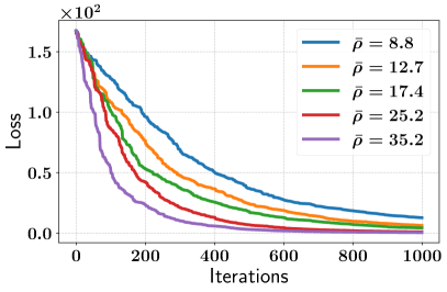
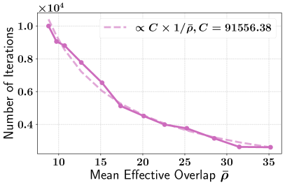
Figure 1: Influence of mean effective overlap $\macc@depth\char 1\relax\frozen@everymath{\macc@group}\macc@set@skewchar\macc@nested@a 111{\rho}$ in controlled low-rank projection $\mathbf{M}$ for randomized quadratic minimization with a dense Hessian. Left: Loss curves with different $\macc@depth\char 1\relax\frozen@everymath{\macc@group}\macc@set@skewchar\macc@nested@a 111{\rho}$ values. Right: Required number of iterations to reach the same loss, with a fitted dotted line illustrating the inverse proportional trend.

Problem Setup. To empirically confirm that the strong impact of the effective overlap $\rho$ (Definition 3.9) on convergence, we design the following experiment. We fix the problem dimension to $d=256$ and construct a rank-$64$ Hessian whose eigenvalues decay linearly from $10$ to $1$. We then introduce a parameter $\gamma\in[0,1]$ to manually adjust $\rho$ by selecting how many of Hessian eigenvectors (specifically, the random-$\lceil s\gamma\rceil$ eigenvectors, where $s=\mathrm{srank}(\mathbf{M})$) are used. The remaining eigenvectors are randomly generated and orthogonalized against those selected, thereby controlling the effective overlap.

Figure 1 highlights the strong interplay between the mean effective overlap $\macc@depth\char 1\relax\frozen@everymath{\macc@group}\macc@set@skewchar\macc@nested@a 111{\rho}$ and convergence speed. In the left panel, higher $\macc@depth\char 1\relax\frozen@everymath{\macc@group}\macc@set@skewchar\macc@nested@a 111{\rho}$ consistently yields faster convergence. In the right panel, we plot the number of iterations required to reach the same loss level as the slowest-converging case at $10^{4}$ iterations, shown as a function of $\macc@depth\char 1\relax\frozen@everymath{\macc@group}\macc@set@skewchar\macc@nested@a 111{\rho}$. A finer sampling of $\lambda$ provides clearer evidence that a larger $\macc@depth\char 1\relax\frozen@everymath{\macc@group}\macc@set@skewchar\macc@nested@a 111{\rho}$ reduces the number of iterations required to meet this reference loss. These observations align closely with Theorem 3.10, which states that convergence speed is inversely proportional to $\macc@depth\char 1\relax\frozen@everymath{\macc@group}\macc@set@skewchar\macc@nested@a 111{\rho}$ (up to a constant $C$), thereby corroborating our theoretical claims. A detailed description of the experimental setup and procedure can be found in Appendix E.1.1.

4.2 Comparison of Low-Dimensional Constraints: Practical Implementations

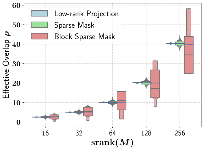
Figure 2: Effective overlap $\rho$ for different methods under a block-diagonal Hessian with heterogeneous eigenspectra. Each boxen plot shows the distribution of effective overlap across 1000 trials for a given $\mathrm{srank}(M)$. The horizontal blue dashed lines indicate the mean effective overlap for each method. The same figure presented in log-scale and strip plot are provided in Appendix F.1.

We now explore three practical approaches to incorporate low-dimensional structure into the matrix $\mathbf{M}$ and examine their behavior. Specifically, we consider:

1. Low-rank projection: $\mathbf{M}=\mathbf{U}\mathbf{U}^{\top}$, where $\mathbf{U}\in\mathbb{R}^{d\times s}$ is a random orthogonal matrix of rank $s<d$.

2. Sparse masking: $\mathbf{M}=\mathrm{diag}(\mathbf{m})$, where $\mathbf{m}=(m_{1},\ldots,m_{d})$ and $m_{i}\sim\mathrm{Bernoulli}(p),p\in(0,1)$.

3. Block sparse masking: $\mathbf{M}=\mathrm{diag}(\mathbf{m})$, but partition the parameters into $N$ blocks $\{B_{1},\ldots,B_{N}\}$. For a mask $\mathbf{m}=(m_{1},\cdots,m_{d})\in\mathbb{R}^{d}$, we set $m_{i}=1$ if $i\in B_{j}$ where $j$ is uniformly sampled at random from $[N]$ (This is reminiscent of block coordinate descent).

Problem Setup. To more closely mirror the behavior of neural network training, we adopt a block-diagonal Hessian with heterogeneous eigenspectra. Prior studies (Collobert, 2004; Zhang et al., 2024b, c) have shown, both theoretically and empirically, that neural network Hessians can be approximated by a block-diagonal matrix, with each dense block exhibiting a distinct eigenvalue distribution. Accordingly, we set the problem dimension to $d=1024$ and partition $\mathbf{H}$ into $16$ diagonal blocks (each of rank $16$). The eigenvalues in each block are set by randomly choosing a reference from $\{10,40,70,100\}$ and sampling each eigenvalue as an integer within $\pm 2$ of it.

To investigate a range of stable ranks $\mathrm{srank}(\mathbf{M})$, we systematically the hyperparameters of each method in a straightforward manner. Specifically, for the low-rank projection, we directly set the rank of $\mathbf{U}$; for the sparse masking, we choose $p=\mathrm{srank}(\mathbf{M})/d$; and for the block sparse masking, we select $N$ such that $d/N=\mathrm{srank}(\mathbf{M})$. Additional details on the experimental setup can be found in Appendix E.1.2.

Distribution of Effective Overlap. Figure 2 displays the distribution of $\rho$ for each method, based on $1000$ independent samples. Note that two key observations stand out. First, as $\mathrm{srank}(\mathbf{M})$ increases, $\rho$ consistently tends to increase across all methods, aligning with the intuition that a larger stable rank spans a broader subspace and thus leads to higher effective overlap. Second, the mean effective overlap $\macc@depth\char 1\relax\frozen@everymath{\macc@group}\macc@set@skewchar\macc@nested@a 111{\rho}$ remains nearly identical across all three methods, indicating that in purely random substructure scenarios, they perform similarly. This phenomenon is further corroborated by the comparable convergence speed observed in our experiments (see Appendix F.2 for example loss curves).

However, the variance of $\rho$ differs substantially. In particular, block sparse masking exhibits a wider spread of effective overlaps. This behavior arises because the Hessian is block-diagonal, and each block’s eigenspectrum can differ considerably. Consequently, the effective overlap depends heavily on which block is selected at each iteration: choosing a block with large eigenvalues leads to a significantly higher $\rho$ than choosing one dominated by smaller eigenvalues.

This variance pattern underscores a critical insight: a higher variance translates into a greater opportunity to discover more effective substructures, particularly those with larger overlap. As a result, if substructure selection is guided by a heuristic or theoretical principle (rather than being purely random), block sparse masking can achieve a more pronounced performance boost. Moreover, block sparse masking significantly simplifies substructure selection. Concretely, low-rank projection requires identifying a handful of critical directions from uncountably many in the whole parameter space, and also sparse masking must consider an extensive set of coordinate combinations. In contrast, block sparse masking merely requires deciding which pre-defined block to activate, an approach that becomes increasingly advantageous as model size grows.

These two advantages, greater potential for improvement and simpler substructure selection, position block sparse masking as a promising approach for zeroth-order optimization in large-scale neural network training, where both ease of tuning and substantial performance gains are essential.

5 Experiments on Large Language Models

Table 1: Performance of fine-tuning OPT-13B on 1000 examples across various fine-tuning tasks. ICL denotes in-context learning, while FT represents full fine-tuning using first-order Adam (Kingma & Ba, 2015). The best results, excluding FT, are highlighted in bold. Results for methods other than MeZO-BCD are taken from Chen et al. (2024).

Task	SST-2	RTE	CB	BoolQ	WSC	WIC	MultiRC	COPA	ReCoRD	SQuAD	DROP
Task type	———————— classification ————————							– multiple choice –		— generation —
Zero-shot	$58.8$	$59.6$	$46.4$	$59.0$	$38.5$	$55.0$	$46.9$	$80.0$	$81.0$	$46.2$	$14.6$
ICL	$87.0$	$62.1$	$57.1$	$66.9$	$39.4$	$50.5$	$53.1$	$87.0$	$\mathbf{82.3}$	$75.9$	$29.5$
MeZO	$91.3$	$68.2$	$66.1$	$68.1$	$61.5$	$59.4$	$59.4$	$88.0$	$81.3$	$81.8$	$31.3$
LoZO	$91.7$	$70.4$	$69.6$	$71.9$	$63.5$	$60.8$	$63.0$	$\mathbf{89.0}$	$81.3$	$\mathbf{84.9}$	$30.7$
MeZO-BCD	$\mathbf{93.0}$	$\mathbf{72.6}$	$\mathbf{71.4}$	$\mathbf{72.4}$	$\mathbf{64.4}$	$\mathbf{61.9}$	$\mathbf{63.2}$	$\mathbf{89.0}$	$\mathbf{81.7}$	$83.9$	$\mathbf{31.4}$
FT	$91.8$	$70.9$	$84.1$	$76.9$	$63.5$	$70.1$	$71.1$	$79.0$	$74.1$	$84.9$	$31.3$

In this section, we investigate the performance comparison of three approaches in LLM fine-tuning scenarios. Specifically, we compare LoZO (Chen et al., 2024) (employing low-rank projection), SparseMeZO (Liu et al., 2024b) (uses sparse masking), and our MeZO-BCD implementation, respectively. For MeZO-BCD, we treat a single transformer decoder layer (encompassing both self-attention and MLP components) as one block. At each optimization step, we either randomly choose the block to be updated or adopt a simple “flip-flop” strategy that alternates between ascending and descending block indices. Further details on MeZO-BCD is provided in Appendix D (refer to Algorithm 1, 2).

Fine-tuning on OPT-13B. To evaluate how MeZO-BCD compares with existing methods, we fine-tune OPT-13B (Zhang et al., 2022a) on multiple tasks, including SuperGLUE (Wang et al., 2019), SQuAD (Rajpurkar et al., 2018), and DROP (Dua et al., 2019). As shown in Table 1, MeZO-BCD surpasses both LoZO and MeZO under these configurations. Notably, this does not imply that MeZO-BCD categorically outperforms its counterparts when extensive hyperparameter tuning is performed on the latter. Rather, our results indicate MeZO-BCD to be at least on par with state-of-the-art ZO methods, suggesting it as a promising method for further exploration in large-scale optimization.

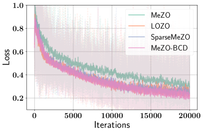
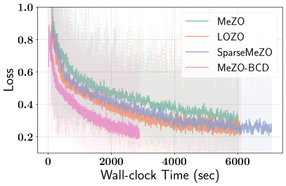
Figure 3: Comparison of training loss curves in terms of iterations (left) and wall-clock time (right) on OPT-1.3B fine-tuning with SST-2 for different methods.

Discussion on Efficiency. Figure 3 compares the convergence of fine-tuning OPT-1.3B (Zhang et al., 2022a) on SST-2 (Socher et al., 2013) in terms of both iterations (left) and wall-clock time (right). While LoZO, SparseMeZO, and MeZO-BCD converge at roughly similar rates per iteration, the differences in wall-clock time per iteration is significant. MeZO and LoZO exhibit similar wall-clock time with SparseMeZO being slightly slower. MeZO-BCD, in contrast is substantially faster by up to $\times\textbf{2.09}$. This benefit arises as MeZO-BCD only needs to sample random perturbations for a single block at each step.

From a memory perspective, MeZO-BCD does not require additional storage compared to MeZO, yielding similar memory benefits. In contrast, LoZO allocates extra memory for subspace maintenance across multiple steps (lazy subspace sampling), and SparseMeZO either stores sparse masks or incurs additional computation to reconstruct them each time. Hence, MeZO-BCD demonstrates superior efficiency in both run-time speed and memory usage.

Additionally, MeZO-BCD can offer unique advantages when combined with stateful optimizers such as Adam or momentum-based methods. Inspired by BAdam (Luo et al., 2024), one could optimize a selected block for a fixed number of steps while maintaining optimizer states only for that block, thereby significantly reducing memory overhead. Although we leave such exploration for future work, this possibility further highlights the efficiency advantages of MeZO-BCD in optimizing large foundation models.

6 Conclusion and Limitations

In this work, we introduced a unified theoretical framework for zeroth-order optimization that reveals how low-dimensional constraints, characterized by stable rank and effective overlap, reduce gradient noise, accelerate convergence, and enhance generalization. Empirical studies validated this framework and highlighted the potential of block coordinate descent, particularly due to its higher variance in effective overlap. Furthermore, we showed that block coordinate descent (MeZO-BCD) is a promising solution for large-scale ZO optimization, offering improved efficiency while achieving performance comparable to existing alternatives in fine-tuning LLM tasks. Despite these advances, several challenges remain as limitations: searching better block-selection strategies, exploring richer structural constraints, and incorporating adaptive gradients, which we leave as future work.

Impact Statements

This paper presents work whose goal is to advance the field of Machine Learning. There are may be potential societal consequences of our work. Specifically, with the growing use cases of the LLM fine-tuning, detailed insights on the ZO and potential efficient alternatives as well proposed in the paper, would help reduce the carbon footprint of such services.

Supplementary Materials

Appendix A Related Works

Convergence and Generalization in Zeroth-order optimization.

Theoretical analysis of zeroth-order (ZO) optimization has been an active research area, with extensive work on its convergence properties across various settings. Early studies established fundamental complexity results for both first-order and zeroth-order methods using Gaussian smoothing (Ghadimi & Lan, 2013). Later, optimal convergence bounds for zeroth-order stochastic gradient descent (SGD) were derived for convex objectives (Duchi et al., 2015) and extended to Gaussian-smoothing-based approaches (Nesterov & Spokoiny, 2017). In nonconvex settings, variance-reduced ZO optimization methods such as ZO-SVRG and ZO-SPIDER were introduced to improve convergence rates and function query efficiency (Ji et al., 2019). More recent works have analyzed ZO optimization under finite-difference, linear interpolation, and various smoothing schemes (Berahas et al., 2022), while others have investigated its behavior in non-smooth regimes, providing sample complexity bounds (Zhang et al., 2020; Davis et al., 2022) and demonstrating that non-smooth ZO optimization is not necessarily more difficult than the smooth case (Rando et al., 2023; Kornowski & Shamir, 2024).

Beyond convergence, the generalization properties of ZO optimization remain underexplored. While existing theoretical studies primarily focus on convergence rates and complexity bounds, fewer works provide a rigorous understanding of how zeroth-order methods generalize in high-dimensional settings. Recent efforts have applied stability-based analyses to first-order optimization, revealing the role of noise in controlling generalization error (Hardt et al., 2016; Lei, 2023). However, extending such frameworks to ZO optimization poses unique challenges due to the inherently higher variance of zeroth-order gradient estimates. Some studies have begun addressing this issue, examining stability bounds for ZO methods (Liu et al., 2024a), but a comprehensive theoretical framework connecting structured perturbations to both convergence and generalization is still lacking.

Fine-tuning Large Language Models with Zeroth-order Optimization.

Zeroth-order (ZO) optimization, a long-standing technique in conventional machine learning (Spall, 1992; Ghadimi & Lan, 2013), was first explored for large language model (LLM) fine-tuning by MeZO (Malladi et al., 2023). By generating perturbations dynamically using random seeds, MeZO eliminates the need to store large perturbation matrices, significantly reducing memory overhead. This allows ZO optimization to operate with memory requirements comparable to inference. While MeZO provides theoretical guarantees, suggesting that scaling the learning rate with respect to the problem dimension ensures dimension-free convergence, this approach inherently results in slow convergence.

Several approaches have been proposed to improve the efficiency of ZO optimization. MeZO-SVRG (Gautam et al., 2024) integrates the SVRG algorithm to reduce gradient variance, leading to faster convergence and improved fine-tuning performance. SparseMeZO (Liu et al., 2024b) enhances computational efficiency by updating only a subset of parameters, while Fisher-informed sparsity (Guo et al., 2024) prioritizes updates based on Fisher information. A benchmarking study (Zhang et al., 2024d) evaluates various ZO methods, including SGD, SignSGD, and Adam. More recently, LOZO (Chen et al., 2024) introduced low-rank perturbations, leveraging the low intrinsic dimensionality of gradients in LLMs to improve convergence and fine-tuning performance.

Building on these works, this work develops a unified theoretical framework that explains how structured perturbations improve both convergence and generalization in ZO optimization. Through this perspective, block coordinate descent (BCD) is identified as an effective structured perturbation strategy, and its advantages are validated through theoretical analysis and empirical evaluation.

Appendix B Proof of Convergence

In this section, we provide the convergence analysis in details. To this end, we revisit our zeroth-order gradient estimator and the update rule.

$$\widehat{\mathbf{g}}_{t} =\frac{\mathcal{L}_{\mathcal{B}_{t}}(\bm{\theta}_{t}+\mu\mathbf{M}_{t}\mathbf{u}_{t})-\mathcal{L}_{\mathcal{B}_{t}}(\bm{\theta}_{t}-\mu\mathbf{M}_{t}\mathbf{u}_{t})}{2\mu}\mathbf{M}_{t}\mathbf{u}_{t}$$

$$\bm{\theta}_{t+1} =\bm{\theta}_{t}-\alpha\widehat{\mathbf{g}}_{t}$$

where $\mathcal{L}_{\mathcal{B}_{t}}(\bm{\theta}_{t})\coloneqq\frac{1}{|\mathcal{B}_{t}|}\sum\limits_{i\in\mathcal{B}_{t}}\mathcal{L}(\bm{\theta}_{t};\mathbf{z}_{i})$ is the loss function evaluated over the minibatch sample $\mathcal{B}_{t}$ at time $t$.

B.1 Preliminary

Gaussian Smoothing.

The zeroth-order gradient estimate $\widehat{\mathbf{g}}_{t}$ is unbiased estimator of the following smoothed loss.

$$\mathcal{L}_{\mu}(\bm{\theta}) \coloneqq\mathbb{E}_{\mathbf{u}\sim\mathcal{N}(\bm{0},\mathbf{I}_{d})}\big{[}\mathcal{L}(\bm{\theta}+\mu\mathbf{u})\big{]}$$

$$\mathcal{L}_{\mu,\mathbf{M}_{t}}(\bm{\theta}) \coloneqq\mathbb{E}_{\mathbf{u}\sim\mathcal{N}(\bm{0},\mathbf{I}_{d})}\big{[}\mathcal{L}(\bm{\theta}+\mu\mathbf{M}_{t}\mathbf{u})\big{]}$$

Note that $\mathcal{L}_{\mu}$ approaches to the original loss $\mathcal{L}$ as $\mu\rightarrow 0$. This indicates that the estimation error between $\mathcal{L}_{\mu}$ and $\mathcal{L}$ or the distance of gradients between $\nabla\mathcal{L}_{\mu}$ and $\nabla\mathcal{L}$ would depend on the smoothing parameter $\mu$.

Lemma B.1 (Alignment of Smoothed Gradients).

The following inner product could be lower-bounded as follows.

$$\big{\langle}\nabla\mathcal{L}_{\mu}(\bm{\theta}),\nabla\mathcal{L}_{\mu,\mathbf{M}_{t}}(\bm{\theta})\big{\rangle} \geq\|\nabla\mathcal{L}_{\mu}(\bm{\theta})\|^{2}-\|\nabla\mathcal{L}_{\mu}(\bm{\theta})\|\mu L\sqrt{2(d+s)}$$

Proof.

By the definition, we have

$$\|\nabla\mathcal{L}_{\mu,\mathbf{M}_{t}}(\bm{\theta})-\nabla\mathcal{L}_{\mu}(\bm{\theta})\| =\Big{\|}\mathbb{E}_{\mathbf{u}}\big{[}\nabla\mathcal{L}(\bm{\theta}+\mu\mathbf{M}_{t}\mathbf{u})-\mathbb{E}_{\mathbf{u}}\big{[}\nabla\mathcal{L}(\bm{\theta}+\mu\mathbf{u})\big{]}\Big{\|}$$

$$=\Big{\|}\mathbb{E}_{\mathbf{u}}\big{[}\nabla\mathcal{L}(\bm{\theta}+\mu\mathbf{M}_{t}\mathbf{u})-\nabla\mathcal{L}(\bm{\theta}+\mu\mathbf{u})\big{]}\Big{\|}$$

$$\leq\mathbb{E}_{\mathbf{u}}\big{[}\big{\|}\nabla\mathcal{L}(\bm{\theta}+\mu\mathbf{M}_{t}\mathbf{u})-\nabla\mathcal{L}(\bm{\theta}+\mu\mathbf{u})\big{\|}\big{]}$$

$$\leq\mu L\mathbb{E}_{\mathbf{u}}\big{[}\|(\mathbf{M}_{t}-\mathbf{I}_{d})\mathbf{u}\|\big{]}$$

$$\leq\mu L\sqrt{\mathrm{Tr}\Big{(}(\mathbf{M}_{t}-\mathbf{I}_{d})^{\top}(\mathbf{M}_{t}-\mathbf{I}_{d})\Big{)}}$$

We let

$$R\coloneqq\mathrm{Tr}\Big{(}(\mathbf{M}_{t}-\mathbf{I}_{d})^{\top}(\mathbf{M}_{t}-\mathbf{I}_{d})\Big{)}$$

for simplicity. For the positive semi-definite matrix $\mathbf{M}_{t}$ with $\mathrm{srank}(\mathbf{M}_{t})\leq s\ll d$, we have

$$R =\mathrm{Tr}\Big{(}(\mathbf{M}_{t}-\mathbf{I}_{d})^{\top}(\mathbf{M}_{t}-\mathbf{I}_{d})\Big{)}$$

$$=\|\mathbf{M}_{t}-\mathbf{I}_{d}\|_{F}^{2}$$

$$\leq(\|\mathbf{M}_{t}\|_{F}+\|\mathbf{I}_{d}\|)^{2}$$

$$\leq 2\|\mathbf{M}_{t}\|_{F}^{2}+2\|\mathbf{I}_{d}\|_{F}^{2}$$

$$=2(d+s)$$

Under the maximal difference $\mu L\sqrt{2(d+s)}$ between $\nabla\mathcal{L}_{\mu,\mathbf{M}_{t}}(\bm{\theta})$ and $\nabla\mathcal{L}_{\mu}(\bm{\theta})$, the inner product could be easily lower-bounded by

$$\big{\langle}\nabla\mathcal{L}_{\mu}(\bm{\theta}),\nabla\mathcal{L}_{\mu,\mathbf{M}_{t}}(\bm{\theta})\big{\rangle} \geq\|\nabla\mathcal{L}_{\mu}(\bm{\theta})\|^{2}-\|\nabla\mathcal{L}_{\mu}(\bm{\theta})\|\mu L\sqrt{2(d+s)}$$

∎

B.2 Technical Lemmas for Matrix Calculus

Lemma B.2 (Trace of Matrix Product).

For positive semi-definite matrices $\mathbf{A},\mathbf{B}\in\mathbb{R}^{d\times d}$, the following holds.

$$\mathrm{Tr}(\mathbf{AB})\leq\mathrm{Tr}(\mathbf{A})\mathrm{Tr}(\mathbf{B})$$

Proof.

Let $\mathbf{v}_{i}$ be an orthonormal basis for $\mathbf{B}$ and $\{\lambda_{i}\}_{i=1}^{d}$ be corresponding eigenvalues. Then, we have

$$\mathrm{Tr}(\mathbf{AB})=\sum\limits_{i=1}^{d}\langle\mathbf{AB}\mathbf{v}_{i},\mathbf{v}_{i}\rangle=\sum\limits_{i=1}^{d}\lambda_{i}\langle\mathbf{A}\mathbf{v}_{i},\mathbf{v}_{i}\rangle=\max\limits_{i\in[d]}\lambda_{i}\mathrm{Tr}(\mathbf{A})\leq\mathrm{Tr}(\mathbf{A})\mathrm{Tr}(\mathbf{B})$$

∎

Lemma B.3 (Nesterov & Spokoiny (2017)).

Let $\mathbf{u}\sim\mathcal{N}(\bm{0},\mathbf{I}_{d})$. Then, the expectation of the moments satisfies

$$\mathbb{E}\big{[}\|\mathbf{u}\|] =1$$

$$\mathbb{E}\big{[}\|\mathbf{u}\|^{2}] =d$$

$$\mathbb{E}\big{[}\|\mathbf{u}\|^{n}] \leq(d+n)^{n/2}$$

for $n\geq 2$.

Lemma B.4 ($n$-th Moments of Quadratic Forms for $n=1,2,3,$ and $4$ (Magnus et al., 1978)).

Let $\mathbf{u}\sim\mathcal{N}(\bm{0},\mathbf{I}_{d})$ and $\mathbf{A}$ be a positive semi-definite matrix. Then, the expectation of the folllowings are

$$\mathbb{E}\Big{[}\mathbf{u}^{\mathsf{T}}\mathbf{A}\mathbf{u}\Big{]} =\mathrm{Tr}(\mathbf{A})$$

$$\mathbb{E}\Big{[}\big{(}\mathbf{u}^{\mathsf{T}}\mathbf{A}\mathbf{u}\big{)}^{2}\Big{]} =(\mathrm{Tr}(\mathbf{A}))^{2}+2\mathrm{Tr}(\mathbf{A}^{2})\leq 3\mathrm{Tr}(\mathbf{A})^{2}$$

$$\mathbb{E}\Big{[}(\mathbf{u}^{\top}\mathbf{A}\mathbf{u})^{3}\Big{]} =\mathrm{Tr}(A)^{3}+6\mathrm{Tr}(\mathbf{A})\mathrm{Tr}(\mathbf{A}^{2})+8\mathrm{Tr}(\mathbf{A}^{3})\leq 15\mathrm{Tr}(\mathbf{A})^{3}$$

$$\mathbb{E}\Big{[}\big{(}\mathbf{u}^{\mathsf{T}}\mathbf{A}\mathbf{u}\big{)}^{4}\Big{]} =(\mathrm{Tr}(\mathbf{A}))^{4}+32\mathrm{Tr}(\mathbf{A})\mathrm{Tr}(\mathbf{A}^{3})+12\big{(}\mathrm{Tr}(\mathbf{A}^{2})\big{)}^{2}+12\big{(}\mathrm{Tr}(\mathbf{A})\big{)}^{2}\mathrm{Tr}(\mathbf{A}^{2})+48\mathrm{Tr}(\mathbf{A}^{4})$$

$$\leq 105\mathrm{Tr}(\mathbf{A})^{4}$$

where the inequalities come from Lemma B.2.

Lemma B.5.

Let $\mathbf{u}\sim\mathcal{N}(\bm{0},\mathbf{I}_{d})$ and $\mathbf{Q}\in\mathbb{R}^{d\times d}$ be an arbitrary matrix. For any vector $\mathbf{a}=(a_{1},a_{2},\cdots,a_{d})\in\mathbb{R}^{d}$, it should hold that

$$\mathbb{E}\big{[}\|\langle\mathbf{a},\mathbf{Qu}\rangle\mathbf{Qu}\|^{2}] =\mathrm{Tr}(\mathbf{Q}\mathbf{Q}^{\mathsf{T}})\|\mathbf{Q}^{\mathsf{T}}\mathbf{a}\|^{2}+2\mathbf{a}^{\mathsf{T}}(\mathbf{Q}\mathbf{Q}^{\mathsf{T}})^{2}\mathbf{a}$$

Proof.

Let $\mathbf{X}=\mathbf{Qu}$ and $\bm{\Sigma}=\mathbf{Q}\mathbf{Q}^{\mathsf{T}}$. Since $\mathbf{u}\sim\mathcal{N}(\bm{0},\mathbf{I}_{d})$, we have $\mathbf{X}\sim\mathcal{N}(\bm{0},\bm{\Sigma})$. Note that $\mathbf{X}$ is $d$-dimensional random vector with $\mathbf{X}=(X_{1},X_{2},\cdots,X_{d})$. Also, the quantity to be expected could be re-written as

$$\|\langle\mathbf{a},\mathbf{Qu}\rangle\mathbf{Qu}\|^{2} =(\mathbf{a}^{\mathsf{T}}\mathbf{X})^{2}\|\mathbf{X}\|^{2}$$

$$=\left(\sum\limits_{i,j}a_{i}a_{j}X_{i}X_{j}\right)\left(\sum\limits_{k}X_{k}^{2}\right)$$

$$=\sum\limits_{i,j,k}a_{i}a_{j}X_{i}X_{j}X_{k}^{2}$$

Note that all we need to derive is $\mathbb{E}[X_{i}X_{j}X_{k}^{2}]$. Since $\mathbf{X}$ follows $\mathcal{N}(\bm{0},\bm{\Sigma})$ distribution, it should hold that $X_{i}$, $X_{j}$, and $X_{k}$ follow $\mathcal{N}(0,\Sigma_{ii})$, $\mathcal{N}(0,\Sigma_{jj})$, and $\mathcal{N}(0,\Sigma_{kk})$, respectively. Thanks to Isserlis’ theorem (Isserlis, 1918) or also known as Wick’s probability theorem (Wick, 1950), we have

$$\mathbb{E}\big{[}X_{i}X_{j}X_{k}^{2}\big{]} =\mathbb{E}\big{[}X_{i}X_{j}X_{k}X_{k}\big{]}$$

$$=\mathbb{E}\big{[}X_{i}X_{j}\big{]}\mathbb{E}\big{[}X_{k}X_{k}\big{]}+\mathbb{E}\big{[}X_{i}X_{k}\big{]}\mathbb{E}\big{[}X_{j}X_{k}\big{]}+\mathbb{E}\big{[}X_{i}X_{k}\big{]}\mathbb{E}\big{[}X_{j}X_{k}\big{]}$$

$$=\mathbb{E}\big{[}X_{i}X_{j}\big{]}\mathbb{E}\big{[}X_{k}^{2}\big{]}+2\mathbb{E}\big{[}X_{i}X_{k}\big{]}\mathbb{E}\big{[}X_{j}X_{k}\big{]}$$

$$=\Sigma_{ij}\Sigma_{kk}+2\Sigma_{ik}\Sigma_{jk}$$

due to the fact $\mathbf{X}\sim\mathcal{N}(\bm{0},\bm{\Sigma})$ and $\bm{\Sigma}=[\Sigma_{mn}]$ for $1\leq m,n\leq d$. Arranging all items, we have

$$\mathbb{E}\big{[}\|\langle\mathbf{a},\mathbf{Qu}\rangle\mathbf{Qu}\|^{2}\big{]} =\sum\limits_{i,j,k}a_{i}a_{j}\mathbb{E}\big{[}X_{i}X_{j}X_{k}^{2}\big{]}$$

$$=\sum\limits_{i,j,k}a_{i}a_{j}\big{(}\Sigma_{ij}\Sigma_{kk}+2\Sigma_{ik}\Sigma_{jk}\big{)}$$

$$=\underbrace{\sum\limits_{i,j,k}a_{i}a_{j}\Sigma_{ij}\Sigma_{kk}}_{T_{1}}+\underbrace{2\sum\limits_{i,j,k}a_{i}a_{j}\Sigma_{ik}\Sigma_{jk}}_{T_{2}}$$

We first compute $T_{1}$. Note that $\Sigma_{kk}$ in $T_{1}$ only depends on the index $k$, thus we have

$$T_{1} =\sum\limits_{i,j,k}a_{i}a_{j}\Sigma_{ij}\Sigma_{kk}$$

$$=\left(\sum\limits_{k=1}^{d}\Sigma_{kk}\right)\left(\sum\limits_{i,j}a_{i}a_{j}\Sigma_{ij}\right)$$

$$=\mathrm{Tr}(\bm{\Sigma})\mathbf{a}^{\mathsf{T}}\bm{\Sigma}\mathbf{a}$$

$$=\mathrm{Tr}\big{(}\mathbf{Q}\mathbf{Q}^{\mathsf{T}}\big{)}\mathbf{a}^{\mathsf{T}}\mathbf{Q}\mathbf{Q}^{\mathsf{T}}\mathbf{a}$$

$$=\mathrm{Tr}\big{(}\mathbf{Q}\mathbf{Q}^{\mathsf{T}}\big{)}\big{\|}\mathbf{Q}^{\mathsf{T}}\mathbf{a}\big{\|}^{2}$$

Now, we compute $T_{2}$. Note that for a fixed $k\in[d]$, $\sum_{i=1}^{d}a_{i}\Sigma_{ik}=[\bm{\Sigma}\mathbf{a}]_{k}$ holds by the definition of matrix multiplication. Hence, we have

$$T_{2} =2\sum\limits_{i,j,k}a_{i}a_{j}\Sigma_{ik}\Sigma_{jk}$$

$$=2\sum\limits_{k=1}^{d}\sum\limits_{i,j}a_{i}\Sigma_{ik}a_{j}\Sigma_{jk}$$

$$=2\sum\limits_{k=1}^{d}\left(\sum\limits_{i=1}^{d}a_{i}\Sigma_{ik}\right)\left(\sum\limits_{j=1}^{d}a_{j}\Sigma_{jk}\right)$$

$$=2\sum\limits_{k=1}^{d}[\bm{\Sigma}\mathbf{a}]_{k}^{2}$$

$$=2\|\bm{\Sigma}\mathbf{a}\|^{2}$$

$$=2\mathbf{a}^{\mathsf{T}}\bm{\Sigma}^{2}\mathbf{a}$$

$$=2\mathbf{a}^{\mathsf{T}}\big{(}\mathbf{Q}\mathbf{Q}^{\mathsf{T}}\big{)}^{2}\mathbf{a}$$

Combining $T_{1}$ and $T_{2}$, we finally obtain

$$\mathbb{E}\big{[}\|\langle\mathbf{a},\mathbf{Qu}\rangle\mathbf{Qu}\|^{2}] =\mathrm{Tr}(\mathbf{Q}\mathbf{Q}^{\mathsf{T}})\|\mathbf{Q}^{\mathsf{T}}\mathbf{a}\|^{2}+2\mathbf{a}^{\mathsf{T}}(\mathbf{Q}\mathbf{Q}^{\mathsf{T}})^{2}\mathbf{a}$$

∎

B.3 Technical Lemmas for Gaussian Smoothed Loss

For completeness of the paper, we include several lemmas already known in zeroth-order optimization literature.

Lemma B.6.

Let $\mathcal{L}_{\mu}(\bm{\theta})=\mathbb{E}\big{[}\mathcal{L}(\bm{\theta}+\mu\mathbf{u})\big{]}$ for some positive $\mu>0$. Then, the following holds.

$$\|\nabla\mathcal{L}_{\mu}(\bm{\theta}_{t})-\nabla\mathcal{L}(\bm{\theta}_{t})\| \leq\frac{\mu L(d+3)^{3/2}}{2}$$

$$\|\nabla\mathcal{L}(\bm{\theta}_{t})\|^{2} \leq\frac{\mu^{2}L^{2}(d+3)^{3}}{2}+2\|\nabla\mathcal{L}_{\mu}(\bm{\theta}_{t})\|^{2}$$

Proof.

Since $\mathcal{L}$ is $L$-smooth, we have for $\mathbf{u}\sim\mathcal{N}(\bm{0},\mathbf{I}_{d})$

$$\mathcal{L}(\bm{\theta}_{t}+\mu\mathbf{u}) \leq\mathcal{L}(\bm{\theta}_{t})+\mu\nabla\mathcal{L}(\bm{\theta}_{t})^{\mathsf{T}}\mathbf{u}+\frac{\mu^{2}L}{2}\|\mathbf{u}\|^{2}.$$

Thus, the distance between $\nabla\mathcal{L}_{\mu}(\bm{\theta}_{t})$ and $\nabla\mathcal{L}(\bm{\theta}_{t})$ can be bounded as

$$\|\nabla\mathcal{L}_{\mu}(\bm{\theta}_{t})-\nabla\mathcal{L}(\bm{\theta}_{t})\| =\frac{1}{Z}\left\|\int_{\mathbf{u}}\left(\frac{\mathcal{L}(\bm{\theta}_{t}+\mu\mathbf{u})-\mathcal{L}(\bm{\theta}_{t})}{\mu}-\nabla\mathcal{L}(\bm{\theta}_{t})\right)\mathbf{u}e^{-\frac{1}{2}\|\mathbf{u}\|^{2}}\mathrm{d}\mathbf{u}\right\|$$

$$=\frac{1}{Z}\left\|\int_{\mathbf{u}}\left(\frac{\mathcal{L}(\bm{\theta}_{t}+\mu\mathbf{u})-\mathcal{L}(\bm{\theta}_{t})-\mu\langle\nabla\mathcal{L}(\bm{\theta}_{t}),\mathbf{u}\rangle}{\mu}\right)\mathbf{u}e^{-\frac{1}{2}\|\mathbf{u}\|^{2}}\mathrm{d}\mathbf{u}\right\|$$

$$\leq\frac{1}{Z}\int_{\mathbf{u}}\left|\frac{\mathcal{L}(\bm{\theta}_{t}+\mu\mathbf{u})-\mathcal{L}(\bm{\theta}_{t})-\mu\langle\nabla\mathcal{L}(\bm{\theta}_{t}),\mathbf{u}\rangle}{\mu}\right|\|\mathbf{u}\|e^{-\frac{1}{2}\|\mathbf{u}\|^{2}}\mathrm{d}\mathbf{u}$$

$$\leq\frac{1}{Z}\int_{\mathbf{u}}\frac{\mu L}{2}\|\mathbf{u}\|^{3}e^{-\frac{1}{2}\|\mathbf{u}\|^{2}}\mathrm{d}\mathbf{u}$$

$$\leq\frac{\mu L(d+3)^{3/2}}{2}$$

where the second inequality comes from the fact $\mathbb{E}[\langle\mathbf{a},\mathbf{u}\rangle\mathbf{u}]=\mathbf{a}$ for any vector $\mathbf{a}\in\mathbb{R}^{d}$. By triangle inequality and Young’s inequality, we have

$$\|\nabla\mathcal{L}(\bm{\theta}_{t})\|^{2} \leq 2\|\nabla\mathcal{L}_{\mu}(\bm{\theta}_{t})-\nabla\mathcal{L}(\bm{\theta}_{t})\|^{2}+\|\nabla\mathcal{L}_{\mu}(\bm{\theta}_{t})\|^{2}$$

$$\leq\frac{\mu^{2}L^{2}(d+3)^{3}}{2}+2\|\nabla\mathcal{L}_{\mu}(\bm{\theta}_{t})\|^{2}$$

∎

Lemma B.7 (Expected Norm of $\widehat{\mathbf{g}}_{t}$).

The expected norm of structured zeroth-order gradient is bounded by

$$\mathbb{E}\big{[}\|\widehat{\mathbf{g}}_{t}\|\big{]}^{2}\leq\mathbb{E}\big{[}\|\widehat{\mathbf{g}}_{t}\|^{2}\big{]} \leq\frac{15\mu^{2}L^{2}s^{3}}{2}+4(s+2)\left(\|\nabla\mathcal{L}(\bm{\theta}_{t})\|^{2}+\frac{\sigma^{2}}{B}\right)$$

Proof.

By the definition of $\widehat{\mathbf{g}}_{t}$ and $L$-smoothness, we have

$$\|\widehat{\mathbf{g}}_{t}\|^{2} =\left\|\frac{\mathcal{L}_{\mathcal{B}_{t}}(\bm{\theta}_{t}+\mu\mathbf{M}_{t}\mathbf{u}_{t})-\mathcal{L}_{\mathcal{B}_{t}}(\bm{\theta}_{t}-\mu\mathbf{M}_{t}\mathbf{u}_{t})}{2\mu}\mathbf{M}_{t}\mathbf{u}_{t}\right\|^{2}$$

$$\leq\frac{2}{\mu^{2}}\left\|\Big{(}\mathcal{L}_{\mathcal{B}_{t}}(\bm{\theta}_{t}+\mu\mathbf{M}_{t}\mathbf{u}_{t})-\mathcal{L}_{\mathcal{B}_{t}}(\bm{\theta}_{t})-\mu\langle\nabla\mathcal{L}_{\mathcal{B}_{t}}(\bm{\theta}_{t}),\mathbf{M}_{t}\mathbf{u}_{t}\rangle\Big{)}\mathbf{M}_{t}\mathbf{u}_{t}\right\|^{2}+2\big{\|}\langle\nabla\mathcal{L}_{\mathcal{B}_{t}}(\bm{\theta}_{t}),\mathbf{M}_{t}\mathbf{u}_{t}\rangle\mathbf{M}_{t}\mathbf{u}_{t}\big{\|}^{2}$$

$$\leq\frac{\mu^{2}L^{2}}{2}\|\mathbf{M}_{t}\mathbf{u}_{t}\|^{6}+2\big{\|}\langle\nabla\mathcal{L}_{\mathcal{B}_{t}}(\bm{\theta}_{t}),\mathbf{M}_{t}\mathbf{u}_{t}\rangle\mathbf{M}_{t}\mathbf{u}_{t}\big{\|}^{2}$$

Note that the first term can be bounded as follows.

$$\mathbb{E}\big{[}\|\mathbf{M}_{t}\mathbf{u}_{t}\|^{2}\big{]} =\mathbb{E}\big{[}\mathbf{u}_{t}^{\top}\mathbf{M}_{t}^{2}\mathbf{u}_{t}\big{]}=\mathrm{Tr}(\mathbf{M}_{t}^{2})\leq s$$

$$\mathbb{E}\big{[}\|\mathbf{M}_{t}\mathbf{u}_{t}\|^{6}\big{]} =\mathbb{E}\big{[}(\mathbf{u}_{t}^{\top}\mathbf{M}_{t}^{2}\mathbf{u}_{t})^{3}\big{]}$$

$$\leq 15\mathrm{Tr}(\mathbf{M}_{t}^{2})^{3}$$

$$\leq 15s^{3}$$

under Lemma B.4 and Assumption 3.4. Therefore, we have

$$\mathbb{E}_{\mathbf{u}_{t}}\big{[}\|\widehat{\mathbf{g}}_{t}\|^{2}\big{]} =\frac{\mu^{2}L^{2}}{2}\mathbb{E}\big{[}\|\mathbf{M}_{t}\mathbf{u}_{t}\|^{6}\big{]}+2\mathbb{E}\Big{[}\big{\|}\langle\nabla\mathcal{L}_{\mathcal{B}_{t}}(\bm{\theta}_{t}),\mathbf{M}_{t}\mathbf{u}_{t}\rangle\mathbf{M}_{t}\mathbf{u}_{t}\big{\|}^{2}\Big{]}$$

$$\leq\frac{15\mu^{2}L^{2}s^{3}}{2}+2(s+2)\|\nabla\mathcal{L}_{\mathcal{B}_{t}}(\bm{\theta}_{t})\|^{2}$$

where we use Lemma B.3 and Lemma B.5. Lastly, taking the expectations with respect to all randomness, we get

$$\mathbb{E}\big{[}\|\widehat{\mathbf{g}}_{t}\|^{2}\big{]} \leq\frac{15\mu^{2}L^{2}s^{3}}{2}+2(s+2)\mathbb{E}_{\mathcal{D}}\big{[}\|\nabla\mathcal{L}_{\mathcal{B}_{t}}(\bm{\theta}_{t})\|^{2}\big{]}$$

$$\leq\frac{15\mu^{2}L^{2}s^{3}}{2}+4(s+2)\left(\|\nabla\mathcal{L}(\bm{\theta}_{t})\|^{2}+\frac{\sigma^{2}}{B}\right)$$

using the condition (C-$2$). ∎

B.4 Proof of Theorem 3.6

By the $L$-smooth loss property, we have

$$\mathcal{L}(\bm{\theta}_{t+1}+\mu\mathbf{u}) \leq\mathcal{L}(\bm{\theta}_{t}+\mu\mathbf{u})+\langle\nabla\mathcal{L}(\bm{\theta}_{t}+\mu\mathbf{u}),\bm{\theta}_{t+1}-\bm{\theta}_{t}\rangle+\frac{L}{2}\|\bm{\theta}_{t+1}-\bm{\theta}_{t}\|^{2}$$

Taking the expectation for both sides yields that

$$\underbrace{\mathbb{E}_{\mathbf{u}}\big{[}\mathcal{L}(\bm{\theta}_{t+1}+\mu\mathbf{u})\big{]}}_{\mathcal{L}_{\mu}(\bm{\theta}_{t+1})} \leq\mathbb{E}_{\mathbf{u}}\Big{[}\mathcal{L}(\bm{\theta}_{t}+\mu\mathbf{u})+\langle\nabla\mathcal{L}(\bm{\theta}_{t}+\mu\mathbf{u}),\bm{\theta}_{t+1}-\bm{\theta}_{t}\rangle+\frac{L}{2}\|\bm{\theta}_{t+1}-\bm{\theta}_{t}\|^{2}\Big{]}$$

$$=\mathcal{L}_{\mu}(\bm{\theta}_{t})-\alpha\langle\nabla\mathcal{L}_{\mu}(\bm{\theta}_{t}),\widehat{\mathbf{g}}_{t}\rangle+\frac{\alpha^{2}L}{2}\|\widehat{\mathbf{g}}_{t}\|^{2}$$

Again, by expectation with respect to $\mathbf{u}_{t}$, we have

$$\mathcal{L}_{\mu}(\bm{\theta}_{t+1}) \leq\mathcal{L}_{\mu}(\bm{\theta}_{t})-\alpha\big{\langle}\nabla\mathcal{L}_{\mu}(\bm{\theta}_{t}),\nabla\mathcal{L}_{\mu,\mathbf{M}_{t}}(\bm{\theta}_{t})\big{\rangle}+\frac{\alpha^{2}L}{2}\mathbb{E}_{\mathbf{u}_{t}}\big{[}\|\widehat{\mathbf{g}}_{t}\|^{2}\big{]}$$

$$\leq\mathcal{L}_{\mu}(\bm{\theta}_{t})-\alpha\Bigg{(}\|\nabla\mathcal{L}_{\mu}(\bm{\theta})\|^{2}-\|\nabla\mathcal{L}_{\mu}(\bm{\theta})\|\mu L\sqrt{2(d+s)}\Bigg{)}+\frac{\alpha^{2}L}{2}\mathbb{E}_{\mathbf{u}_{t}}\big{[}\|\widehat{\mathbf{g}}_{t}\|^{2}\big{]}$$

$$\leq\mathcal{L}_{\mu}(\bm{\theta}_{t})-\alpha\|\nabla\mathcal{L}_{\mu}(\bm{\theta}_{t})\|^{2}+\frac{\alpha}{2}\|\nabla\mathcal{L}_{\mu}(\bm{\theta}_{t})\|^{2}+\alpha\mu^{2}L^{2}(d+s)+\frac{\alpha^{2}L}{2}\mathbb{E}_{\mathbf{u}_{t}}\big{[}\|\widehat{\mathbf{g}}_{t}\|^{2}\big{]}$$

By Lemma B.7, we have

$$\mathcal{L}_{\mu}(\bm{\theta}_{t+1}) \leq\mathcal{L}_{\mu}(\bm{\theta}_{t})-\frac{\alpha}{2}\|\nabla\mathcal{L}_{\mu}(\bm{\theta}_{t})\|^{2}+\frac{\alpha\mu^{2}L^{2}R}{2}+\frac{\alpha^{2}L}{2}\Bigg{(}\frac{15\mu^{2}L^{2}s^{3}}{2}+2(s+2)\left(\|\nabla\mathcal{L}(\bm{\theta}_{t})\|^{2}+\frac{\sigma^{2}}{B}\right)\Bigg{)}$$

Rearranging the inequality, we obtain

$$\frac{\alpha}{4}\|\nabla\mathcal{L}(\bm{\theta}_{t})\|^{2} \leq\frac{\alpha\mu^{2}L^{2}(d+3)^{3}}{8}+\frac{\alpha}{2}\|\nabla\mathcal{L}_{\mu}(\bm{\theta}_{t})\|^{2}$$

$$\leq\frac{\alpha\mu^{2}L^{2}(d+3)^{3}}{8}+\mathcal{L}_{\mu}(\bm{\theta}_{t})-\mathcal{L}_{\mu}(\bm{\theta}_{t+1})+\alpha\mu^{2}L^{2}(d+s)+\frac{15\alpha^{2}\mu^{2}L^{3}s^{3}}{4}$$

$$\quad+\alpha^{2}L(s+2)\|\nabla\mathcal{L}(\bm{\theta}_{t})\|^{2}+\frac{\alpha^{2}L(s+2)\sigma^{2}}{B}$$

We assume the following stepsize condition

$$\alpha \leq\frac{1}{8L(s+2)}.$$

Finally, we have

$$\frac{\alpha}{8}\|\nabla\mathcal{L}(\bm{\theta}_{t})\|^{2} \leq\frac{\alpha\mu^{2}L^{2}(d+3)^{3}}{8}+\mathcal{L}_{\mu}(\bm{\theta}_{t})-\mathcal{L}_{\mu}(\bm{\theta}_{t+1})+\alpha\mu^{2}L^{2}(d+s)+\frac{15\alpha^{2}\mu^{2}L^{3}s^{3}}{4}+\frac{\alpha^{2}L(s+2)\sigma^{2}}{B}$$

Hence, we obtain

$$\|\nabla\mathcal{L}(\bm{\theta}_{t})\|^{2} \leq\mu^{2}L^{2}(d+3)^{3}+\frac{8\big{(}\mathcal{L}_{\mu}(\bm{\theta}_{t})-\mathcal{L}_{\mu}(\bm{\theta}_{t+1})\big{)}}{\alpha}+8\mu^{2}L^{2}(d+s)+30\alpha\mu^{2}L^{3}s^{3}+\frac{8L(s+2)\sigma^{2}}{B}$$

We let $\Delta=\mathcal{L}_{\mu}(\bm{\theta}_{1})-\mathcal{L}_{\mu}(\bm{\theta}^{*})$. Under the smoothing parameter condition $\mu=\mathcal{O}(\frac{1}{L\sqrt{sdT}})$, we finally arrive at

$$\mathbb{E}\Big{[}\frac{1}{T}\sum\limits_{t=1}^{T}\|\nabla\mathcal{L}(\bm{\theta}_{t})\|^{2}\Big{]} \leq\mu^{2}L^{2}(d+3)^{3}+\frac{8\Delta}{\alpha T}+8\mu^{2}L^{2}(d+s)+30\alpha\mu^{2}L^{3}s^{3}+\frac{8\alpha L(s+2)\sigma^{2}}{B}$$

$$\leq\Big{[}\mu^{2}L^{2}d^{3}+\frac{\Delta}{\alpha T}+\mu^{2}L^{2}s^{2}\Big{]}\mathcal{O}\Big{(}\frac{1}{T}\Big{)}+\mathcal{O}\Big{(}\frac{\sigma^{2}}{B}\Big{)}$$

$$\leq\mathcal{O}\Big{(}\frac{d^{2}}{sT}+\frac{s^{2}}{dT}+\frac{\Delta}{\alpha T}+\frac{\sigma^{2}}{B}\Big{)}$$

B.5 Proof of Theorem 3.10

In this section, we provide the convergence analysis with additional assumption on the intrinsic dimension of the loss function.

Lemma B.8.

Let $\mathcal{L}_{\mu}(\bm{\theta})=\mathbb{E}\big{[}\mathcal{L}(\bm{\theta}+\mu\mathbf{u})\big{]}$ for some positive $\mu>0$. Then, with locally low intrinsic dimension, the following holds.

$$\|\nabla\mathcal{L}_{\mu}(\bm{\theta}_{t})-\nabla\mathcal{L}(\bm{\theta}_{t})\| \leq\frac{\sqrt{3}\mu Lr\sqrt{d}}{2}+\frac{\mu L(d+4)\sqrt{d}}{2}\exp(-\frac{c_{1}}{2}d)$$

$$\|\nabla\mathcal{L}(\bm{\theta}_{t})\|^{2} \leq 3\mu^{2}L^{2}r^{2}d+\mu^{2}L^{2}d(d+4)^{2}\exp(-c_{1}d)+2|\nabla\mathcal{L}_{\mu}(\bm{\theta}_{t})\|^{2}$$

Proof.

Let $\mathcal{E}$ be the event such that $\|\bm{\theta}_{t}+\mu\mathbf{u}-\bm{\theta}_{t}\|\leq 2\alpha sG+2\mu\sqrt{d}$. On the event $\mathcal{E}$, by the low intrinsic dimension condition, there exists some matrix $\mathbf{H}(\bm{\theta}_{t})$ such that $\nabla^{2}\mathcal{L}(\bm{\theta}_{t}+\mu\mathbf{u})\preceq\mathbf{H}(\bm{\theta}_{t})$ with $\mathrm{intdim}(\mathbf{H}(\bm{\theta}_{t}))\leq r$. Thus, we have the following inequality

$$\mathcal{L}(\bm{\theta}_{t}+\mu\mathbf{u}) \leq\mathcal{L}(\bm{\theta}_{t})+\mu\nabla\mathcal{L}(\bm{\theta}_{t})^{\top}\mathbf{u}+\frac{\mu^{2}}{2}\mathbf{u}^{\top}\mathbf{H}(\bm{\theta}_{t})\mathbf{u}$$

$$=\mathcal{L}(\bm{\theta}_{t})+\mu\nabla\mathcal{L}(\bm{\theta}_{t})^{\top}\mathbf{u}+\frac{\mu^{2}}{2}\Big{\langle}\mathbf{H}(\bm{\theta}_{t}),\mathbf{u}\mathbf{u}^{\top}\Big{\rangle}$$

Likewise, on the event $\mathcal{E}^{c}$, we have

$$\mathcal{L}(\bm{\theta}_{t}+\mu\mathbf{u})\leq\mathcal{L}(\bm{\theta}_{t})+\mu\nabla\mathcal{L}(\bm{\theta}_{t})^{\top}\mathbf{u}+\frac{\mu^{2}L}{2}\|\mathbf{u}\|^{2}$$

By the concentration inequality for (sub-)Gaussian random vector, we have $\mathbb{P}[\mathcal{E}^{c}]\leq\exp(-c_{1}d)$ for some universal constant $c_{1}>0$.

$$\|\nabla\mathcal{L}_{\mu}(\bm{\theta}_{t})-\nabla\mathcal{L}(\bm{\theta}_{t})\| =\|\nabla\mathbb{E}\big{[}\mathcal{L}(\bm{\theta}_{t}+\mu\mathbf{u})\big{]}-\nabla\mathcal{L}(\bm{\theta}_{t})\|$$

$$\leq\Big{\|}\mathbb{E}_{\mathbf{u}}\Big{[}\frac{\mathcal{L}(\bm{\theta}_{t}+\mu\mathbf{u})-\mathcal{L}(\bm{\theta}_{t})}{\mu}\mathbf{u}\Big{]}-\nabla\mathcal{L}(\bm{\theta}_{t})\Big{\|}$$

$$=\Big{\|}\mathbb{E}_{\mathbf{u}}\Big{[}\frac{\mathcal{L}(\bm{\theta}_{t}+\mu\mathbf{u})-\mathcal{L}(\bm{\theta}_{t})-\mu\langle\nabla\mathcal{L}(\bm{\theta}_{t}),\mathbf{u}\rangle}{\mu}\mathbf{u}\Big{]}\Big{\|}$$

$$\leq\mathbb{E}_{\mathbf{u}}\Big{[}\Big{(}\frac{\mathcal{L}(\bm{\theta}_{t}+\mu\mathbf{u})-\mathcal{L}(\bm{\theta}_{t})-\mu\langle\nabla\mathcal{L}(\bm{\theta}_{t}),\mathbf{u}\rangle}{\mu}\Big{)}^{2}\Big{]}^{1/2}\mathbb{E}\big{[}\|\mathbf{u}\|^{2}\big{]}^{1/2}$$

The first term could be bounded as

$$\mathbb{E}_{\mathbf{u}}\Big{[}\Big{(}\frac{\mathcal{L}(\bm{\theta}_{t}+\mu\mathbf{u})-\mathcal{L}(\bm{\theta}_{t})-\mu\langle\nabla\mathcal{L}(\bm{\theta}_{t}),\mathbf{u}\rangle}{\mu}\Big{)}^{2}\Big{]} \leq\frac{\mu^{2}}{4}\mathbb{E}_{\mathbf{u}}\Big{[}\big{(}\mathbf{u}^{\top}\mathbf{H}(\bm{\theta}_{t})\mathbf{u}\big{)}^{2}\Big{]}+\exp(-c_{1}d)\frac{\mu^{2}L^{2}}{4}\mathbb{E}_{\mathbf{u}}\big{[}\|\mathbf{u}\|^{4}\big{]}$$

$$\leq\frac{3\mu^{2}L^{2}r^{2}}{4}+\frac{\mu^{2}L^{2}(d+4)^{2}}{4}\exp(-c_{1}d)$$

where we use Lemma B.3 and Lemma B.4 as

$$\mathbb{E}\Big{[}\big{(}\mathbf{u}^{\top}\mathbf{H}(\bm{\theta}_{t})\mathbf{u}\big{)}^{2}\Big{]} \leq 3\mathrm{Tr}\big{(}\mathbf{H}(\bm{\theta}_{t})\big{)}^{2}\leq 3L^{2}r^{2}$$

$$\mathbb{E}\big{[}\|\mathbf{u}\|^{2}\big{]} \leq d$$

Therefore, we could obtain

$$\|\nabla\mathcal{L}_{\mu}(\bm{\theta}_{t})-\nabla\mathcal{L}(\bm{\theta}_{t})\| \leq\Big{(}\frac{\sqrt{3}\mu Lr}{2}+\frac{\mu L(d+4)}{2}\exp(-\frac{c_{1}}{2}d)\Big{)}\sqrt{d}$$

$$=\frac{\sqrt{3}\mu Lr\sqrt{d}}{2}+\frac{\mu L(d+4)\sqrt{d}}{2}\exp(-\frac{c_{1}}{2}d)$$

Hence, we further obtain

$$\|\nabla\mathcal{L}(\bm{\theta}_{t})\|^{2} \leq 2\|\nabla\mathcal{L}_{\mu}(\bm{\theta}_{t})-\nabla\mathcal{L}(\bm{\theta}_{t})\|^{2}+2\|\nabla\mathcal{L}(\bm{\theta}_{t})\|^{2}$$

$$\leq 3\mu^{2}L^{2}r^{2}d+\mu^{2}L^{2}d(d+4)^{2}\exp(-c_{1}d)+2|\nabla\mathcal{L}_{\mu}(\bm{\theta}_{t})\|^{2}$$

∎

Lemma B.9.

The following inequality holds

$$\mathcal{L}_{\mu}(\bm{\theta}_{t+1})\leq\mathcal{L}_{\mu}(\bm{\theta}_{t})-\alpha\Big{\langle}\nabla\mathcal{L}_{\mu}(\bm{\theta}_{t}),\nabla\mathcal{L}_{\mu,\mathbf{M}_{t}}(\bm{\theta}_{t})\Big{\rangle}+\frac{\alpha^{2}}{2}\Big{\langle}\mathbb{E}\big{[}\widehat{\mathbf{g}}_{t}\widehat{\mathbf{g}}_{t}^{\top}\big{]},\mathbf{H}(\bm{\theta}_{t})\Big{\rangle}$$

$$\qquad+\frac{\alpha^{2}}{2}\Big{\langle}\mathbb{E}\Big{[}\widehat{\mathbf{g}}_{t}\widehat{\mathbf{g}}_{t}^{\top}\!\cdot\!\mathbb{I}(\mathcal{E}^{c})\Big{]},L\!\cdot\!\mathbf{I}_{d}-\mathbf{H}(\bm{\theta}_{t})\Big{\rangle},$$

$$\frac{\alpha^{2}}{2}\Big{\langle}\mathbb{E}\Big{[}\widehat{\mathbf{g}}_{t}\widehat{\mathbf{g}}_{t}^{\top}\!\cdot\!\mathbb{I}(\mathcal{E}^{c})\Big{]},L\!\cdot\!\mathbf{I}_{d}-\mathbf{H}(\bm{\theta}_{t})\Big{\rangle}\leq\alpha^{2}L\Big{(}37\mu^{2}L^{2}s^{3}+42s\Big{(}\|\nabla\mathcal{L}(\bm{\theta}_{t})\|^{2}+\frac{\sigma^{2}}{B}\Big{)}\Big{)}\exp\Big{(}-\frac{s}{2}\Big{)}$$

Proof.

Let $\mathcal{E}$ be the event that $\|\bm{\theta}_{t+1}-\bm{\theta}_{t}\|\leq 2\alpha sG+2\mu\sqrt{d}$. On $\mathcal{E}$, we have

$$\mathcal{L}(\bm{\theta}_{t+1}+\mu\mathbf{u}) \leq\mathcal{L}(\bm{\theta}_{t}+\mu\mathbf{u})-\alpha\langle\nabla\mathcal{L}(\bm{\theta}_{t}+\mu\mathbf{u}),\widehat{\mathbf{g}}_{t}\rangle+\frac{1}{2}\Big{\langle}\widehat{\mathbf{g}}_{t}\widehat{\mathbf{g}}_{t}^{\top},\mathbf{H}(\bm{\theta}_{t})\Big{\rangle}$$

On $\mathcal{E}^{c}$, we have for $L$-smooth loss,

$$\mathcal{L}(\bm{\theta}_{t+1}+\mu\mathbf{u}) \leq\mathcal{L}(\bm{\theta}_{t}+\mu\mathbf{u})-\alpha\langle\nabla\mathcal{L}(\bm{\theta}_{t}+\mu\mathbf{u}),\widehat{\mathbf{g}}_{t}\rangle+\frac{L}{2}\|\widehat{\mathbf{g}}_{t}\|^{2}$$

Combining two inequalities along the expectations with respect to $\mathbf{u}$ and $\mathbf{u}_{t}$, we have

$$\mathcal{L}_{\mu}(\bm{\theta}_{t+1}) \leq\mathcal{L}_{\mu}(\bm{\theta}_{t})-\alpha\Big{\langle}\nabla\mathcal{L}_{\mu}(\bm{\theta}_{t}),\nabla\mathcal{L}_{\mu,\mathbf{M}_{t}}(\bm{\theta}_{t})\Big{\rangle}+\frac{\alpha^{2}}{2}\Big{\langle}\mathbb{E}\big{[}\widehat{\mathbf{g}}_{t}\widehat{\mathbf{g}}_{t}^{\top}\!\cdot\!\mathbb{I}(\mathcal{E})\big{]},\mathbf{H}(\bm{\theta}_{t})\Big{\rangle}$$

$$\qquad+\frac{\alpha^{2}L}{2}\mathbb{E}\big{[}\|\widehat{\mathbf{g}}_{t}\|^{2}\!\cdot\!\mathbb{I}(\mathcal{E}^{c})\big{]}$$

$$=\mathcal{L}_{\mu}(\bm{\theta}_{t})-\alpha\Big{\langle}\nabla\mathcal{L}_{\mu}(\bm{\theta}_{t}),\nabla\mathcal{L}_{\mu,\mathbf{M}_{t}}(\bm{\theta}_{t})\Big{\rangle}+\frac{\alpha^{2}}{2}\Big{\langle}\mathbb{E}\big{[}\widehat{\mathbf{g}}_{t}\widehat{\mathbf{g}}_{t}^{\top}\big{]},\mathbf{H}(\bm{\theta}_{t})\Big{\rangle}$$

$$\qquad+\frac{\alpha^{2}}{2}\Big{\langle}\mathbb{E}\Big{[}\widehat{\mathbf{g}}_{t}\widehat{\mathbf{g}}_{t}^{\top}\!\cdot\!\mathbb{I}(\mathcal{E}^{c})\Big{]},L\!\cdot\!\mathbf{I}_{d}-\mathbf{H}(\bm{\theta}_{t})\Big{\rangle}$$

The last term could be bounded as

$$\frac{\alpha^{2}}{2}\Big{\langle}\mathbb{E}\Big{[}\widehat{\mathbf{g}}_{t}\widehat{\mathbf{g}}_{t}^{\top}\cdot\mathbb{I}(\mathcal{E}^{c})\Big{]},L\!\cdot\!\mathbf{I}_{d}-\mathbf{H}(\bm{\theta}_{t})\Big{\rangle} \leq\alpha^{2}L\mathbb{E}\Big{[}\|\widehat{\mathbf{g}}_{t}\|^{2}\cdot\mathbb{I}(\mathcal{E}^{c})\Big{]}$$

$$=\alpha^{2}L\mathbb{E}\Big{[}\|\widehat{\mathbf{g}}_{t}\|^{4}\Big{]}^{1/2}\mathbb{P}[\mathcal{E}^{c}]^{1/2}.$$

The first term could be computed as

$$\|\widehat{\mathbf{g}}_{t}\|^{4} \leq\left\|\frac{\mathcal{L}_{\mathcal{B}_{t}}(\bm{\theta}_{t}+\mu\mathbf{M}_{t}\mathbf{u}_{t})-\mathcal{L}_{\mathcal{B}_{t}}(\bm{\theta}_{t}-\mu\mathbf{M}_{t}\mathbf{u}_{t})}{2\mu}\mathbf{M}_{t}\mathbf{u}_{t}\right\|^{4}$$

$$\leq\frac{2}{\mu^{4}}\left\|\Big{(}\mathcal{L}_{\mathcal{B}_{t}}(\bm{\theta}_{t}+\mu\mathbf{M}_{t}\mathbf{u}_{t})-\mathcal{L}_{\mathcal{B}_{t}}(\bm{\theta}_{t})-\mu\langle\nabla\mathcal{L}_{\mathcal{B}_{t}}(\bm{\theta}_{t}),\mathbf{M}_{t}\mathbf{u}_{t}\rangle\Big{)}\mathbf{M}_{t}\mathbf{u}_{t}\right\|^{4}+4\big{\|}\langle\nabla\mathcal{L}_{\mathcal{B}_{t}}(\bm{\theta}_{t}),\mathbf{M}_{t}\mathbf{u}_{t}\rangle\mathbf{M}_{t}\mathbf{u}_{t}\big{\|}^{4}$$

$$\leq\frac{\mu^{4}L^{4}}{8}\|\mathbf{M}_{t}\mathbf{u}_{t}\|^{12}+4\Big{\|}\langle\nabla\mathcal{L}_{\mathcal{B}_{t}}(\bm{\theta}_{t}),\mathbf{M}_{t}\mathbf{u}_{t}\rangle\mathbf{M}_{t}\mathbf{u}_{t}\Big{\|}^{4}$$

The expectation of each term could be bounded as

$$\mathbb{E}\big{[}\|\mathbf{M}_{t}\mathbf{u}_{t}\|^{12}\big{]} \leq 10395s^{6}$$

$$\mathbb{E}\big{[}\|\langle\nabla\mathcal{L}_{\mathcal{B}_{t}}(\bm{\theta}_{t}),\mathbf{M}_{t}\mathbf{u}_{t}\rangle\mathbf{M}_{t}\mathbf{u}_{t}\|^{4}\big{]} \leq 105s^{2}\|\nabla\mathcal{L}_{\mathcal{B}_{t}}(\bm{\theta}_{t})\|^{4}$$

Thus, we have

$$\mathbb{E}\big{[}\|\widehat{\mathbf{g}}_{t}\|^{4}\big{]} \leq\frac{10395\mu^{4}L^{4}s^{6}}{8}+420s^{2}\|\nabla\mathcal{L}_{\mathcal{B}_{t}}(\bm{\theta}_{t})\|^{4}$$

$$\mathbb{E}\big{[}\|\widehat{\mathbf{g}}_{t}\|^{4}\big{]}^{1/2} \leq 37\mu^{2}L^{2}s^{3}+21s\|\nabla\mathcal{L}_{\mathcal{B}_{t}}(\bm{\theta}_{t})\|^{2}$$

$$\leq 37\mu^{2}L^{2}s^{3}+42s(\|\nabla\mathcal{L}(\bm{\theta}_{t})\|^{2}+\frac{\sigma^{2}}{B})$$

Now, we compute the probability of the event $\mathcal{E}^{c}$. Note that on the event $\mathcal{E}^{c}$, we have

$$2\alpha sG+\mu\sqrt{d}\leq\|\bm{\theta}_{t+1}-\bm{\theta}_{t}\| =\alpha\|\widehat{\mathbf{g}}_{t}\|\leq\alpha G\|\mathbf{M}_{t}\mathbf{u}_{t}\|^{2}$$

Therefore, we should compute the probability such that

$$\|\mathbf{M}_{t}\mathbf{u}_{t}\|^{2}\geq 2s+\frac{\mu\sqrt{d}}{\alpha G}$$

Using Hanson-Wright inequality (Hanson & Wright, 1971; Wright, 1973), it is easy to check that $\mathbb{P}[\mathcal{E}^{c}]\leq\exp(-s/2)$ holds. Combining all the items, we finally have

$$\frac{\alpha^{2}}{2}\Big{\langle}\mathbb{E}\Big{[}\widehat{\mathbf{g}}_{t}\widehat{\mathbf{g}}_{t}^{\top}\!\cdot\!\mathbb{I}(\mathcal{E}^{c})\Big{]},L\!\cdot\!\mathbf{I}_{d}-\mathbf{H}(\bm{\theta}_{t})\Big{\rangle} \leq\alpha^{2}L\Big{(}37\mu^{2}L^{2}s^{3}+42s\Big{(}\|\nabla\mathcal{L}(\bm{\theta}_{t})\|^{2}+\frac{\sigma^{2}}{B}\Big{)}\Big{)}\exp\Big{(}-\frac{s}{2}\Big{)}$$

∎

Lemma B.10.

The following inequality holds

$$\mathbb{E}\big{[}\widehat{\mathbf{g}}_{t}^{\top}\mathbf{H}(\bm{\theta}_{t})\widehat{\mathbf{g}}_{t}\big{]} \leq 13\mu^{2}L^{3}s^{2}\rho+9L\rho\Big{(}\|\nabla\mathcal{L}(\bm{\theta}_{t})\|^{2}+\frac{\sigma^{2}}{B}\Big{)}.$$

Proof.

By the definition of $\widehat{\mathbf{g}}_{t}$, we have

$$\mathbb{E}\Big{[}\widehat{\mathbf{g}}_{t}^{\top}\mathbf{H}(\bm{\theta}_{t})\widehat{\mathbf{g}}_{t}\Big{]} =\frac{1}{4\mu^{2}}\mathbb{E}\Big{[}\Big{(}\mathcal{L}_{\mathcal{B}_{t}}(\bm{\theta}_{t}+\mu\mathbf{M}_{t}\mathbf{u}_{t})-\mathcal{L}_{\mathcal{B}_{t}}(\bm{\theta}_{t}-\mu\mathbf{M}_{t}\mathbf{u}_{t})\Big{)}^{2}\mathbf{u}_{t}^{\top}\mathbf{M}_{t}\mathbf{H}(\bm{\theta}_{t})\mathbf{M}_{t}\mathbf{u}_{t}\Big{]}$$

$$\leq\frac{1}{4\mu^{2}}\mathbb{E}\Big{[}\Big{(}\mathcal{L}_{\mathcal{B}_{t}}(\bm{\theta}_{t}+\mu\mathbf{M}_{t}\mathbf{u}_{t})-\mathcal{L}_{\mathcal{B}_{t}}(\bm{\theta}_{t}-\mu\mathbf{M}_{t}\mathbf{u}_{t})\Big{)}^{4}\Big{]}^{1/2}\mathbb{E}\Big{[}\big{(}\mathbf{u}_{t}^{\top}\mathbf{M}_{t}\mathbf{H}(\bm{\theta}_{t})\mathbf{M}_{t}\mathbf{u}_{t}\big{)}^{2}\Big{]}^{1/2}$$

$$\leq\frac{\sqrt{3}L\rho}{4\mu^{2}}\mathbb{E}\Big{[}\Big{(}\mathcal{L}_{\mathcal{B}_{t}}(\bm{\theta}_{t}+\mu\mathbf{M}_{t}\mathbf{u}_{t})-\mathcal{L}_{\mathcal{B}_{t}}(\bm{\theta}_{t}-\mu\mathbf{M}_{t}\mathbf{u}_{t})\Big{)}^{4}\Big{]}^{1/2}$$

The function difference could be handled as

$$\mathcal{L}_{\mathcal{B}_{t}}(\bm{\theta}_{t}+\mu\mathbf{M}_{t}\mathbf{u}_{t})-\mathcal{L}_{\mathcal{B}_{t}}(\bm{\theta}_{t}-\mu\mathbf{M}_{t}\mathbf{u}_{t}) \leq\mu^{2}L\|\mathbf{M}_{t}\mathbf{u}_{t}\|^{2}+2\mu\big{\langle}\nabla\mathcal{L}_{\mathcal{B}_{t}}(\bm{\theta}_{t}),\mathbf{M}_{t}\mathbf{u}_{t}\big{\rangle}$$

Therefore, the fourth exponent of this difference can be bounded by

$$\mathbb{E}\Big{[}\Big{(}\mathcal{L}_{\mathcal{B}_{t}}(\bm{\theta}_{t}+\mu\mathbf{M}_{t}\mathbf{u}_{t})-\mathcal{L}_{\mathcal{B}_{t}}(\bm{\theta}_{t}-\mu\mathbf{M}_{t}\mathbf{u}_{t})\Big{)}^{4}\Big{]} \leq\mathbb{E}\Big{[}\Big{(}\mu^{2}L\|\mathbf{M}_{t}\mathbf{u}_{t}\|^{2}+2\mu\big{\langle}\nabla\mathcal{L}_{\mathcal{B}_{t}}(\bm{\theta}_{t}),\mathbf{M}_{t}\mathbf{u}_{t}\big{\rangle}\Big{)}^{4}\Big{]}$$

$$\leq 8\mathbb{E}\Big{[}\mu^{8}L^{4}\|\mathbf{M}_{t}\mathbf{u}_{t}\|^{8}+16\mu^{4}\big{\langle}\nabla\mathcal{L}_{\mathcal{B}_{t}}(\bm{\theta}_{t}),\mathbf{M}_{t}\mathbf{u}_{t}\big{\rangle}^{4}\Big{]}$$

$$\leq 8\mu^{8}L^{4}\mathbb{E}\big{[}\|\mathbf{M}_{t}\mathbf{u}_{t}\|^{8}\big{]}+128\mu^{4}\mathbb{E}\big{[}\langle\nabla\mathcal{L}_{\mathcal{B}_{t}}(\bm{\theta}_{t}),\mathbf{M}_{t}\mathbf{u}_{t}\rangle^{4}\big{]}$$

$$\leq 840\mu^{8}L^{4}s^{4}+384\mu^{4}\|\nabla\mathcal{L}_{\mathcal{B}_{t}}(\bm{\theta}_{t})\|^{4}$$

Also, by the definition of effective overlap in Definition 3.9, we have

$$\mathrm{Tr}(\mathbf{M}_{t}\mathbf{H}(\bm{\theta}_{t})\mathbf{M}_{t})=L\rho_{t}$$

Hence, we obtain

$$\mathbb{E}\big{[}\widehat{\mathbf{g}}_{t}^{\top}\mathbf{H}(\bm{\theta}_{t})\widehat{\mathbf{g}}_{t}\big{]} \leq\frac{\sqrt{3}L\rho_{t}}{4\mu^{2}}\Big{(}\sqrt{840}\mu^{4}L^{2}s^{2}+\sqrt{384}\mu^{2}\|\nabla\mathcal{L}_{\mathcal{B}_{t}}(\bm{\theta}_{t})\|^{2}\Big{)}$$

$$\leq 13\mu^{2}L^{3}s^{2}\rho_{t}+9L\rho_{\text{max}}\Big{(}\|\nabla\mathcal{L}(\bm{\theta}_{t})\|^{2}+\frac{\sigma^{2}}{B}\Big{)}$$

∎

Proof of Theorem 3.10

Proof.

We have

$$\mathcal{L}_{\mu}(\bm{\theta}_{t+1}) \leq\mathcal{L}_{\mu}(\bm{\theta}_{t})-\frac{\alpha}{2}\|\nabla\mathcal{L}_{\mu}(\bm{\theta}_{t})\|^{2}+\alpha\mu^{2}L^{2}(d+s)+\frac{\alpha^{2}}{2}\Big{(}13\mu^{2}L^{3}s^{2}\rho_{t}+9L\rho_{\text{max}}\Big{(}\|\nabla\mathcal{L}(\bm{\theta}_{t})\|^{2}+\frac{\sigma^{2}}{B}\Big{)}\Big{)}$$

$$\qquad+\alpha^{2}L\Big{(}37\mu^{2}L^{2}s^{3}+42s(\|\nabla\mathcal{L}(\bm{\theta}_{t})\|^{2}+\frac{\sigma^{2}}{B})\Big{)}\exp(-s/2)$$

By Lemma B.8, we have

$$\frac{\alpha}{4}\|\nabla\mathcal{L}(\bm{\theta}_{t})\|^{2} \leq\frac{3\alpha\mu^{2}L^{2}r^{2}d}{16}+\frac{\alpha}{2}\|\nabla\mathcal{L}_{\mu}(\bm{\theta}_{t})\|^{2}$$

$$\leq\frac{3\alpha\mu^{2}L^{2}r^{2}d}{16}+\mathcal{L}_{\mu}(\bm{\theta}_{t})-\mathcal{L}_{\mu}(\bm{\theta}_{t+1})+\alpha\mu^{2}L^{2}(d+s)+\frac{13\alpha^{2}\mu^{2}L^{3}s^{2}\rho_{t}}{2}+\frac{9\alpha^{2}L\rho_{\text{max}}}{2}\|\nabla\mathcal{L}(\bm{\theta}_{t})\|^{2}$$

$$\qquad+\frac{9\alpha^{2}L\rho_{\text{max}}\sigma^{2}}{2B}+37\alpha^{2}\mu^{2}L^{3}s^{3}\exp\big{(}-s/2\big{)}+42\alpha^{2}Ls\exp\big{(}-s/2\big{)}\|\nabla\mathcal{L}(\bm{\theta}_{t})\|^{2}$$

$$\qquad+\frac{42\alpha^{2}Ls\sigma^{2}}{B}\exp\big{(}-s/2\big{)}$$

By rearranging inequality, we have

$$\Big{(}\frac{\alpha}{4}-\frac{9\alpha^{2}L\rho_{\text{max}}}{2}-42\alpha^{2}Ls\exp(-s/2)\Big{)}\sum\limits_{t=1}^{T}\|\nabla\mathcal{L}(\bm{\theta}_{t})\|^{2} \leq\frac{3\alpha\mu^{2}L^{2}r^{2}d}{16}+\mathcal{L}_{\mu}(\bm{\theta}_{t})-\mathcal{L}_{\mu}(\bm{\theta}_{t+1})+\alpha\mu^{2}L^{2}(d+s)$$

$$\qquad+\frac{13\alpha^{2}L^{3}s^{2}\rho_{t}}{2}+\frac{9\alpha^{2}L\rho_{\text{max}}\sigma^{2}}{2B}+37\alpha^{2}\mu^{2}L^{3}s^{3}\exp(-s/2)$$

$$\qquad+\frac{42\alpha^{2}Ls\sigma^{2}}{B}\exp(-s/2)$$

Under the following parameter condition,

$$\alpha\leq\frac{1}{36L\rho_{\text{max}}+336Ls\exp(-s/2)},$$

$$\frac{\alpha}{8}\|\nabla\mathcal{L}(\bm{\theta}_{t})\|^{2} \leq\frac{3\alpha\mu^{2}L^{2}r^{2}d}{16}+\mathcal{L}_{\mu}(\bm{\theta}_{t})-\mathcal{L}_{\mu}(\bm{\theta}_{t+1})+\alpha\mu^{2}L^{2}(d+s)+\frac{13\alpha^{2}\mu^{2}L^{3}s^{2}\rho_{t}}{2}+\frac{9\alpha^{2}L\rho_{\text{max}}\sigma^{2}}{2B}$$

$$\qquad+37\alpha^{2}\mu^{2}L^{3}s^{3}\exp(-s/2)+\frac{42\alpha^{2}Ls\sigma^{2}}{B}\exp(-s/2)$$

Therefore, we have

$$\|\nabla\mathcal{L}(\bm{\theta}_{t})\|^{2} \leq\frac{3\mu^{2}L^{2}r^{2}d}{2}+\frac{8(\mathcal{L}_{\mu}(\bm{\theta}_{t})-\mathcal{L}_{\mu}(\bm{\theta}_{t+1}))}{\alpha}+8\mu^{2}L^{2}(d+s)+52\alpha\mu^{2}L^{3}s^{2}\rho_{t}+\frac{36\alpha L\rho_{\text{max}}\sigma^{2}}{B}$$

$$\qquad+296\alpha\mu^{2}L^{3}s^{3}\exp(-s/2)+\frac{336\alpha Ls\sigma^{2}}{B}\exp(-s/2)$$

$$\leq\frac{3\mu^{2}L^{2}r^{2}d}{2}+\frac{8(\mathcal{L}_{\mu}(\bm{\theta}_{t})-\mathcal{L}_{\mu}(\bm{\theta}_{t+1}))}{\alpha}+8\mu^{2}L^{2}(d+s)+\frac{13\mu^{2}L^{2}s^{2}\rho_{t}}{9}$$

$$\qquad+\frac{37\mu^{2}L^{2}s^{2}}{42}+\frac{\sigma^{2}}{B}$$

Telescoping the inequality from $t=1$ to $T$ with stepsize condition and $\mu=\mathcal{O}(\frac{1}{L\sqrt{\macc@depth\char 1\relax\frozen@everymath{\macc@group}\macc@set@skewchar\macc@nested@a 111{\rho}dT}})$, we obtain

$$\frac{1}{T}\sum\limits_{t=1}^{T}\|\nabla\mathcal{L}(\bm{\theta}_{t})\|^{2} \leq\frac{3r^{2}}{2\macc@depth\char 1\relax\frozen@everymath{\macc@group}\macc@set@skewchar\macc@nested@a 111{\rho}T}+\frac{8\Delta}{\alpha T}+\frac{8(d+s)}{\macc@depth\char 1\relax\frozen@everymath{\macc@group}\macc@set@skewchar\macc@nested@a 111{\rho}dT}+\frac{13s^{2}}{9dT}+\frac{37s^{2}}{42\macc@depth\char 1\relax\frozen@everymath{\macc@group}\macc@set@skewchar\macc@nested@a 111{\rho}dT}+\frac{\sigma^{2}}{B}$$

$$\leq\mathcal{O}\Big{(}\frac{1}{\macc@depth\char 1\relax\frozen@everymath{\macc@group}\macc@set@skewchar\macc@nested@a 111{\rho}T}\Big{(}r^{2}+\frac{s^{2}}{d}+1\Big{)}+\frac{s^{2}}{dT}+\frac{\Delta}{\alpha T}+\frac{\sigma^{2}}{B}\Big{)}.$$

∎

Appendix C Proof of Generalization Error Bound

In this section, we consider the following online update.

$$\widehat{\nabla}\mathcal{L}(\bm{\theta}_{t};\mathbf{z}_{i_{t}}) =\frac{\mathcal{L}(\bm{\theta}_{t}+\mu\mathbf{M}_{t}\mathbf{u}_{t};\mathbf{z}_{i_{t}})-\mathcal{L}(\bm{\theta}_{t}-\mu\mathbf{M}_{t}\mathbf{u}_{t};\mathbf{z}_{i_{t}})}{2\mu}\mathbf{M}_{t}\mathbf{u}_{t}$$

$$\bm{\theta}_{t+1} =\bm{\theta}_{t}-\alpha_{t}\widehat{\nabla}\mathcal{L}(\bm{\theta}_{t};\mathbf{z}_{i_{t}})$$

For generalization error bound, we employ the uniform stability framework. Note that we define some quantities

$$\mathcal{E}_{t_{0}} =\{\bm{\theta}_{t}=\bm{\theta}_{t_{0}}\}~\text{(the event)}$$

$$\delta_{t} =\|\bm{\theta}_{t}-\bm{\theta}_{t}^{\prime}\|,\quad\Delta_{t}=\mathbb{E}\big{[}\delta_{t}|\mathcal{E}_{t_{0}}\big{]}$$

C.1 Auxiliary Lemmas

Lemma C.1.

For any $t>t_{0}$, the distance between the zeroth-order gradients, evaluated on the same datapoint $\mathbf{z}_{i_{t}}$ but on the different parameters $\bm{\theta}_{t}$ and $\bm{\theta}_{t}^{\prime}$, is bounded as

$$\mathbb{E}\Big{[}\Big{\|}\widehat{\nabla}\mathcal{L}(\bm{\theta}_{t};\mathbf{z}_{i_{t}})-\widehat{\nabla}\mathcal{L}(\bm{\theta}_{t}^{\prime};\mathbf{z}_{i_{t}})\Big{\|}\Big{]} \leq\sqrt{3s}\big{(}4L\rho+\mu Ls\exp(-s/2)\big{)}+L\sqrt{s}\delta_{t}$$

Proof.

For simplicity, we denote $\mathcal{L}(\bm{\theta}_{t};\mathbf{z}_{i_{t}})\eqqcolon\mathcal{L}_{i_{t}}(\bm{\theta}_{t})$. By the definition of zeroth-order gradient estimator, we have

$$\widehat{\nabla}\mathcal{L}_{i_{t}}(\bm{\theta}_{t}) =\frac{\mathcal{L}_{i_{t}}(\bm{\theta}_{t}+\mu\mathbf{M}_{t}\mathbf{u}_{t})-\mathcal{L}_{i_{t}}(\bm{\theta}_{t}-\mu\mathbf{M}_{t}\mathbf{u}_{t})}{2\mu}\mathbf{M}_{t}\mathbf{u}_{t}$$

$$=\frac{\mathcal{L}_{i_{t}}(\bm{\theta}_{t}+\mu\mathbf{M}_{t}\mathbf{u}_{t})-\mathcal{L}_{i_{t}}(\bm{\theta}_{t})-\mu\langle\nabla\mathcal{L}_{i_{t}}(\bm{\theta}_{t}),\mathbf{M}_{t}\mathbf{u}_{t}\rangle}{2\mu}\mathbf{M}_{t}\mathbf{u}_{t}$$

$$\qquad-\frac{\mathcal{L}_{i_{t}}(\bm{\theta}_{t}-\mu\mathbf{M}_{t}\mathbf{u}_{t})-\mathcal{L}_{i_{t}}(\bm{\theta}_{t})-\mu\langle\nabla\mathcal{L}_{i_{t}}(\bm{\theta}_{t}),-\mathbf{M}_{t}\mathbf{u}_{t}\rangle}{2\mu}\mathbf{M}_{t}\mathbf{u}_{t}$$

$$\qquad+\langle\nabla\mathcal{L}_{i_{t}}(\bm{\theta}_{t}),\mathbf{M}_{t}\mathbf{u}_{t}\rangle\mathbf{M}_{t}\mathbf{u}_{t}$$

Therefore, the gradient difference is

$$\widehat{\nabla}\mathcal{L}_{i_{t}}(\bm{\theta}_{t})-\widehat{\nabla}\mathcal{L}_{i_{t}}(\bm{\theta}_{t}^{\prime}) =\frac{\mathcal{L}_{i_{t}}(\bm{\theta}_{t}+\mu\mathbf{M}_{t}\mathbf{u}_{t})-\mathcal{L}_{i_{t}}(\bm{\theta}_{t})-\mu\langle\nabla\mathcal{L}_{i_{t}}(\bm{\theta}_{t}),\mathbf{M}_{t}\mathbf{u}_{t}\rangle}{2\mu}\mathbf{M}_{t}\mathbf{u}_{t}$$

$$\qquad-\frac{\mathcal{L}_{i_{t}}(\bm{\theta}_{t}-\mu\mathbf{M}_{t}\mathbf{u}_{t})-\mathcal{L}_{i_{t}}(\bm{\theta}_{t})-\mu\langle\nabla\mathcal{L}_{i_{t}}(\bm{\theta}_{t}),-\mathbf{M}_{t}\mathbf{u}_{t}\rangle}{2\mu}\mathbf{M}_{t}\mathbf{u}_{t}$$

$$\qquad-\frac{\mathcal{L}_{i_{t}}(\bm{\theta}_{t}^{\prime}+\mu\mathbf{M}_{t}\mathbf{u}_{t})-\mathcal{L}_{i_{t}}(\bm{\theta}_{t}^{\prime})-\mu\langle\nabla\mathcal{L}_{i_{t}}(\bm{\theta}_{t}^{\prime}),\mathbf{M}_{t}\mathbf{u}_{t}\rangle}{2\mu}\mathbf{M}_{t}\mathbf{u}_{t}$$

$$\qquad+\frac{\mathcal{L}_{i_{t}}(\bm{\theta}_{t}^{\prime}-\mu\mathbf{M}_{t}\mathbf{u}_{t})-\mathcal{L}_{i_{t}}(\bm{\theta}_{t}^{\prime})-\mu\langle\nabla\mathcal{L}_{i_{t}}(\bm{\theta}_{t}^{\prime}),-\mathbf{M}_{t}\mathbf{u}_{t}\rangle}{2\mu}\mathbf{M}_{t}\mathbf{u}_{t}$$

$$\qquad+\langle\nabla\mathcal{L}_{i_{t}}(\bm{\theta}_{t})-\nabla\mathcal{L}_{i_{t}}(\bm{\theta}_{t}^{\prime}),\mathbf{M}_{t}\mathbf{u}_{t}\rangle\mathbf{M}_{t}\mathbf{u}_{t}$$

Let $\mathcal{E}$ be the event that $\|\mu\mathbf{M}_{t}\mathbf{u}_{t}\|\leq 2\alpha_{t}sG+2\mu\sqrt{d}$. By Hanson-Wright inequality or Gaussian tail bound, it is easy to check $\mathbb{P}[\mathcal{E}^{c}]\leq\exp(-c_{3}d)$ for some universal constant $c_{3}>0$. On the event $\mathcal{E}$, we have

$$\Bigg{|}\frac{\mathcal{L}_{i_{t}}(\bm{\theta}_{t}+\mu\mathbf{M}_{t}\mathbf{u}_{t})-\mathcal{L}_{i_{t}}(\bm{\theta}_{t})-\mu\big{\langle}\nabla\mathcal{L}_{i_{t}}(\bm{\theta}_{t}),\mathbf{M}_{t}\mathbf{u}_{t}\big{\rangle}}{2\mu}\Bigg{|}\leq\frac{\mu}{4}\mathbf{u}_{t}^{\top}\mathbf{M}_{t}\mathbf{H}(\bm{\theta}_{t})\mathbf{M}_{t}\mathbf{u}_{t}$$

On the event $\mathcal{E}^{c}$, with probability at most $\exp(-c_{3}d)$, we have

$$\Bigg{|}\frac{\mathcal{L}_{i_{t}}(\bm{\theta}_{t}+\mu\mathbf{M}_{t}\mathbf{u}_{t})-\mathcal{L}_{i_{t}}(\bm{\theta}_{t})-\mu\big{\langle}\nabla\mathcal{L}_{i_{t}}(\bm{\theta}_{t}),\mathbf{M}_{t}\mathbf{u}_{t}\big{\rangle}}{2\mu}\Bigg{|}\leq\frac{\mu L}{4}\|\mathbf{M}_{t}\mathbf{u}_{t}\|^{2}$$

Hence, we have

$$\mathbb{E}\Bigg{[}\Bigg{(}\frac{\mathcal{L}_{i_{t}}(\bm{\theta}_{t}+\mu\mathbf{M}_{t}\mathbf{u}_{t})-\mathcal{L}_{i_{t}}(\bm{\theta}_{t})-\mu\big{\langle}\nabla\mathcal{L}_{i_{t}}(\bm{\theta}_{t}),\mathbf{M}_{t}\mathbf{u}_{t}\big{\rangle}}{2\mu}\Bigg{)}^{2}\Bigg{]} \leq\frac{3\mu^{2}L^{2}\rho_{\text{max}}^{2}}{16}+\frac{\mu^{2}L^{2}}{16}\mathbb{E}\big{[}\|\mathbf{M}_{t}\mathbf{u}_{t}\|^{4}\big{]}\exp(-s/4)$$

$$\leq\frac{3\mu^{2}L^{2}\rho_{\text{max}}^{2}}{16}+\frac{3\mu^{2}L^{2}s^{2}}{16}\exp(-s/4)$$

Combining two inequalities, we obtain

$$\mathbb{E}\Bigg{[}\Bigg{\|}\frac{\mathcal{L}_{i_{t}}(\bm{\theta}_{t}+\mu\mathbf{M}_{t}\mathbf{u}_{t})-\mathcal{L}_{i_{t}}(\bm{\theta}_{t})-\mu\langle\nabla\mathcal{L}_{i_{t}}(\bm{\theta}_{t}),\mathbf{M}_{t}\mathbf{u}_{t}\rangle}{2\mu}\mathbf{M}_{t}\mathbf{u}_{t}\Bigg{\|}\Bigg{]}$$

$$\leq~ \mathbb{E}\Bigg{[}\Bigg{(}\frac{\mathcal{L}_{i_{t}}(\bm{\theta}_{t}+\mu\mathbf{M}_{t}\mathbf{u}_{t})-\mathcal{L}_{i_{t}}(\bm{\theta}_{t})-\mu\langle\nabla\mathcal{L}_{i_{t}}(\bm{\theta}_{t}),\mathbf{M}_{t}\mathbf{u}_{t}\rangle}{2\mu}\Bigg{)}^{2}\Bigg{]}^{1/2}\mathbb{E}\big{[}\|\mathbf{M}_{t}\mathbf{u}_{t}\|^{2}\big{]}^{1/2}$$

$$\leq~ \Big{(}\frac{3\mu^{2}L^{2}\rho_{\text{max}}^{2}}{16}+\frac{3\mu^{2}L^{2}s^{2}}{16}\exp(-s/4)\Big{)}^{1/2}s^{1/2}$$

$$\leq~ \frac{\sqrt{3s}}{4}\Big{(}\mu L\rho_{\text{max}}+\mu Ls\exp(-s/2)\Big{)}$$

Hence, the expected distance can be bounded as

$$\mathbb{E}\Big{[}\|\widehat{\nabla}\mathcal{L}_{i_{t}}(\bm{\theta}_{t})-\widehat{\nabla}\mathcal{L}_{i_{t}}(\bm{\theta}_{t}^{\prime})\|\Big{]} \leq\sqrt{3s}\Big{(}\mu L\rho_{\text{max}}+\mu Ls\exp(-s/2)\Big{)}+\mathbb{E}\big{[}\|\langle\nabla\mathcal{L}_{i_{t}}(\bm{\theta}_{t})-\nabla\mathcal{L}_{i_{t}}(\bm{\theta}_{t}^{\prime}),\mathbf{M}_{t}\mathbf{u}_{t}\rangle\mathbf{M}\mathbf{u}_{t}\|]$$

$$\leq\sqrt{3s}\Big{(}\mu L\rho_{\text{max}}+\mu Ls\exp(-s/2)\Big{)}+\|\nabla\mathcal{L}_{i_{t}}(\bm{\theta}_{t})-\nabla\mathcal{L}_{i_{t}}(\bm{\theta}_{t}^{\prime})\|\sqrt{s}$$

$$\leq\sqrt{3s}\Big{(}\mu L\rho_{\text{max}}+\mu Ls\exp(-s/2)\Big{)}+L\sqrt{s}\|\bm{\theta}_{t}-\bm{\theta}_{t}^{\prime}\|$$

$$=\sqrt{3s}\Big{(}\mu L\rho_{\text{max}}+\mu Ls\exp(-s/2)\Big{)}+L\sqrt{s}\delta_{t}$$

∎

Lemma C.2.

The following recursive relation

$$\Delta_{t} \leq(1+\alpha_{t}L\sqrt{s})\Delta_{t}+\alpha_{t}\sqrt{3s}(\mu L\rho_{\text{max}}+\mu Ls\exp(-s/2))+\alpha_{t}\frac{4G\sqrt{s}}{n}$$

Proof.

For any $t>t_{0}$, we have

$$\delta_{t+1} =\big{\|}\bm{\theta}_{t}-\alpha_{t}\widehat{\nabla}\mathcal{L}_{i_{t}}(\bm{\theta}_{t})-\bm{\theta}_{t}^{\prime}+\alpha_{t}\widehat{\nabla}\mathcal{L}_{i_{t}^{\prime}}(\bm{\theta}_{t}^{\prime})\big{\|}$$

$$\leq\|\bm{\theta}_{t}-\bm{\theta}_{t}^{\prime}\|+\alpha_{t}\underbrace{\big{\|}\widehat{\nabla}\mathcal{L}_{i_{t}}(\bm{\theta}_{t})-\widehat{\nabla}\mathcal{L}_{i_{t}^{\prime}}(\bm{\theta}_{t}^{\prime})\big{\|}}_{R_{t}}$$

$$=\delta_{t}+\alpha_{t}R_{t}$$

We consider two cases for recursive relation for $R_{t}$ (in fact, for $\mathbb{E}[R_{t}]$).

Case 1: With probability $1-\dfrac{1}{n}$, we have $i_{t}=i_{t}^{\prime}$ where the same datapoint is sampled at time $t$. By Lemma C.1, we have

$$E[R_{t}] =\mathbb{E}\big{[}\|\widehat{\nabla}\mathcal{L}_{i_{t}}(\bm{\theta}_{t})-\widehat{\nabla}\mathcal{L}_{i_{t}}(\bm{\theta}_{t}^{\prime})\|\big{]}$$

$$\leq\sqrt{3s}\Big{(}\mu L\rho_{\text{max}}+\mu Ls\exp(-s/2)\Big{)}+L\sqrt{s}\Delta_{t}$$

by Lemma C.1.

Case 2: With probability $\dfrac{1}{n}$, we have $i_{t}\neq i_{t}^{\prime}$. Therefore, we obtain

$$\mathbb{E}[R_{t}] =\mathbb{E}\big{[}\|\widehat{\nabla}\mathcal{L}_{i_{t}}(\bm{\theta}_{t})-\widehat{\nabla}\mathcal{L}_{i_{t}^{\prime}}(\bm{\theta}_{t}^{\prime})\|\big{]}$$

$$\leq\mathbb{E}\big{[}\|\widehat{\nabla}\mathcal{L}_{i_{t}}(\bm{\theta}_{t})\|\big{]}+\mathbb{E}\big{[}\widehat{\nabla}\mathcal{L}_{i_{t}^{\prime}}(\bm{\theta}_{t}^{\prime})\|\big{]}$$

$$\leq\sqrt{3s}\Big{(}\mu L\rho_{\text{max}}+\mu Ls\exp(-s/2)\Big{)}+4G\sqrt{s}$$

From two cases, we can derive the recursive relation for $\Delta_{t}$ as

$$\Delta_{t+1} \leq\Delta_{t}+\alpha_{t}\Big{(}1-\frac{1}{n}\Big{)}\Big{(}\sqrt{3s}\Big{(}\mu L\rho_{\text{max}}+\mu Ls\exp(-s/2)\Big{)}+L\sqrt{s}\Delta_{t}\Big{)}+\frac{\alpha_{t}}{n}\Big{(}\sqrt{3s}\Big{(}\mu L\rho_{\text{max}}+\mu Ls\exp(-s/2)\Big{)}+4G\sqrt{s}\Big{)}$$

$$\leq(1+\alpha_{t}L\sqrt{s})\Delta_{t}+\alpha_{t}\sqrt{3s}(\mu L\rho_{\text{max}}+\mu Ls\exp(-s/2))+\alpha_{t}\frac{4G\sqrt{s}}{n}$$

∎

Proof of Theorem 3.14

Proof.

Under the following parameter condition

$$\mu\leq\frac{1}{nL(\rho_{\text{max}}+s\exp(-s/2))},\quad\alpha_{t}\leq\frac{C}{t},$$

we have simpler recursive relation as

$$\Delta_{t+1} \leq\Big{(}1+\alpha_{t}L\sqrt{s}\Big{)}\Delta_{t}+\alpha_{t}\Big{(}\sqrt{3s}\mu L\rho_{\text{max}}+\sqrt{3s}\mu Ls\exp(-s/2)+\frac{4G\sqrt{s}}{n}\Big{)}$$

Solving this inequality yields that

$$\Delta_{T} \leq\Big{(}\sqrt{3s}\mu L\rho_{\text{max}}+\sqrt{3s}\mu Ls\exp(-s/2)+\frac{4G\sqrt{s}}{n}\Big{)}\sum\limits_{t=t_{0}+1}^{T}\alpha_{t}\prod_{j=t+1}^{T}(1+\alpha_{j}L\sqrt{s})$$

$$\leq C\Big{(}\sqrt{3s}\mu L\rho_{\text{max}}+\sqrt{3s}\mu Ls\exp(-s/2)+\frac{4G\sqrt{s}}{n}\Big{)}\sum\limits_{t=t_{0}+1}^{T}\frac{1}{t}\prod_{j=t+1}^{T}\Big{(}1+\frac{CL\sqrt{s}}{j}\Big{)}$$

$$\leq C\Big{(}\sqrt{3s}\mu L\rho_{\text{max}}+\sqrt{3s}\mu Ls\exp(-s/2)+\frac{4G\sqrt{s}}{n}\Big{)}\sum\limits_{t=t_{0}+1}^{T}\frac{1}{t}\prod_{j=t+1}^{T}\exp\Big{(}\frac{CL\sqrt{s}}{j}\Big{)}$$

$$\leq C\Big{(}\sqrt{3s}\mu L\rho_{\text{max}}+\sqrt{3s}\mu Ls\exp(-s/2)+\frac{4G\sqrt{s}}{n}\Big{)}\sum\limits_{t=t_{0}+1}^{T}\frac{1}{t}\exp\Big{(}CL\sqrt{s}\sum\limits_{j=t+1}^{T}\frac{1}{j}\Big{)}$$

$$\leq C\Big{(}\sqrt{3s}\mu L\rho_{\text{max}}+\sqrt{3s}\mu Ls\exp(-s/2)+\frac{4G\sqrt{s}}{n}\Big{)}\sum\limits_{t=t_{0}+1}^{T}\frac{1}{t}\exp\Big{(}CL\sqrt{s}\big{(}\log T-\log t\big{)}\Big{)}$$

$$\leq CT^{CL\sqrt{s}}\Big{(}\sqrt{3s}\mu L\rho_{\text{max}}+\sqrt{3s}\mu Ls\exp(-s/2)+\frac{4G\sqrt{s}}{n}\Big{)}\sum\limits_{t=t_{0}+1}^{T}\frac{1}{t^{CL\sqrt{s}+1}}$$

$$\leq\frac{1}{L\sqrt{s}}\Big{(}\sqrt{3s}\mu L\rho_{\text{max}}+\sqrt{3s}\mu Ls\exp(-s/2)+\frac{4G\sqrt{s}}{n}\Big{)}\Big{(}\Big{(}\frac{T}{t_{0}}\Big{)}^{CL\sqrt{s}}-1\Big{)}$$

$$=\underbrace{\Big{(}\frac{\sqrt{3}+4G}{nL}\Big{)}}_{D}\Big{[}\Big{(}\frac{T}{t_{0}}\Big{)}^{CL\sqrt{s}}-1\Big{]}$$

Let $q\coloneqq CL\sqrt{s}$ and the optimal value $t_{0}^{*}$ which minimizes the RHS of the following inequality

$$\mathbb{E}\big{[}\|\mathcal{L}(\bm{\theta}_{T};\mathbf{z})-\mathcal{L}(\bm{\theta}_{T}^{\prime};\mathbf{z})\|\big{]} \leq\frac{t_{0}}{n}\sup_{\bm{\theta},\mathbf{z}}\mathcal{L}(\bm{\theta};\mathbf{z})+G\Delta_{T}$$

$$\leq\frac{t_{0}}{n}+GD\Big{[}\Big{(}\frac{T}{t_{0}}\Big{)}^{q}-1\Big{]}$$

is given by $t_{0}^{*}=\min\{(nqGDT^{q})^{\frac{1}{1+q}},T\}$. Under the smoothing parameter condition $\mu\leq\frac{1}{nL\rho_{\text{max}}}$, we have

$$\epsilon_{\textnormal{gen}} \leq\frac{q+1}{nq}(nqGDT^{q})^{\frac{1}{1+q}}-GD$$

$$=\frac{q+1}{nq}\Big{[}\frac{qG(\sqrt{3}+4G)}{L}\Big{]}^{\frac{1}{1+q}}T^{1-\frac{1}{1+q}}-\frac{G(\sqrt{3}+4G)}{nL}$$

$$=\frac{q+1}{nq^{\frac{q}{1+q}}}\Big{(}\frac{G(\sqrt{3}+4G)}{L}\Big{)}^{\frac{1}{1+q}}T^{1-\frac{1}{1+q}}-\frac{G(\sqrt{3}+4G)}{nL}$$

$$=\mathcal{O}\Bigg{(}\frac{T^{1-\frac{1}{1+q}}}{n}\Bigg{)},$$

where $q=CL\sqrt{s}$. ∎

Appendix D Detailed Description of MeZO-BCD

MeZO with Block Coordinate Descent (MeZO-BCD) follows a block-wise zeroth-order optimization strategy, where the parameters are partitioned into $N$ disjoint blocks, $\mathbf{B}=\{B_{i}\}_{i=1}^{N}$. In our method, each block corresponds to all the parameters of a single Transformer decoder layer, ensuring structured and efficient updates.

D.1 Block-Wise Zeroth-Order Optimization

At each iteration, instead of updating all parameters simultaneously, MeZO-BCD selects only one block to update. The active block index $j$ is determined based on one of the following update strategies:

• Random permutation-based selection: Instead of sampling blocks independently at random, a random permutation of $[N]$ is precomputed and followed for $N$ steps. After each full cycle, a new random permutation is generated. This ensures that all blocks are updated exactly once per cycle while maintaining randomness.

• Flip-flop selection: The block index oscillates sequentially between $1$ and $N$, ensuring all layers are updated in a cyclic order.

• Ascending order: Blocks are updated sequentially from $1$ to $N$, then restart from $1$.

• Descending order: Blocks are updated sequentially from $N$ to $1$, then restart from $N$.

Among these strategies, random permutation-based and flip-flop selection generally showed better performance in most cases. The random permutation approach ensures that each block is updated exactly once per cycle while avoiding systematic biases introduced by sequential ordering. The flip-flop strategy ensures a balanced coverage of all layers over time. Ascending and descending orders, while systematic, tended to introduce biases in weight updates, increasing the likelihood of converging to a suboptimal solution.

D.2 Efficient Implementation via Block Prefix Matching

In the actual implementation, we efficiently partition the model parameters by maintaining a list of prefixes corresponding to each block. Instead of explicitly storing parameter indices, we apply perturbations only to parameters whose names match a stored prefix. Furthermore, we treat the embedding layers and the language modeling head (lm_head) as a single block, in addition to the Transformer decoder layers. This ensures that parameter updates remain consistent across all critical model components.

For example, in OPT-1.3B, the parameter prefixes used for block partitioning are:

• "model.decoder.layers.0.", "model.decoder.layers.1.", $\dots$, "model.decoder.layers.23."

• "model.decoder.embed_tokens." (Embedding layer)

• "lm_head." (Language model head)

At each training step, the function PerturbParameters applies perturbations only to parameters whose names contain the prefix corresponding to the currently selected block.

D.3 Computational Benefit of Block Updates

A key advantage of MeZO-BCD is that each training step only requires generating a random matrix for a single block. Since random matrix generation is required for zeroth-order gradient estimation, performing this operation on only one block per step significantly reduces computation time.

This efficiency gain is particularly important given that zeroth-order optimization relies solely on forward passes. Unlike first-order optimization, where gradient computation dominates the computational cost, even seemingly small operations such as generating random perturbations can introduce substantial overhead in zeroth-order methods. By restricting perturbation generation to a single Transformer decoder layer per step, MeZO-BCD minimizes this overhead while maintaining low-dimensionally structured updates.

Why BCD is More Effective in Zeroth-Order Optimization.

In first-order (FO) optimization, applying block coordinate descent (BCD) can lead to significant computational and memory inefficiencies. The primary reason is that backpropagation propagates gradients through all subsequent layers, meaning that when updating a block closer to the input layer, the computational and memory cost grows substantially due to the need to compute and store gradients for all proceeding layers.

However, in zeroth-order (ZO) optimization, there is no backpropagation, and the gradient is estimated based solely on the perturbed function evaluations. This means that only the selected block is affected at each step, with no additional computational overhead from later layers. As a result, ZO-BCD fully realizes the ideal efficiency of block-wise updates, allowing purely localized updates without unnecessary computational dependencies. This makes BCD particularly well-suited for ZO, as it achieves the desired reduction in per-step complexity without the typical drawbacks encountered in FO optimization.

D.4 On the Choice of Block Partitioning Granularity

The choice of block granularity is crucial in determining both computational efficiency and optimization behavior. We considered several partitioning strategies:

• Finer partitions: Blocks corresponding to individual nn.Linear layers, or grouping all self-attention modules separately from MLPs.

• Coarser partitions: Merging two consecutive decoder layers into a single block.

Through empirical evaluation, we found that:

• Finer partitions significantly slowed down convergence, likely due to excessive variance in the zeroth-order gradient estimates. The updates became too fragmented, making optimization inefficient.

• Coarser partitions showed no major advantage over learning rate tuning, meaning that increasing the block size did not offer a meaningful improvement in optimization dynamics.

Based on these findings, we standardize one Transformer decoder layer as a single block, balancing efficiency and convergence speed.

Algorithm 1 MeZO with Block Coordinate Descent (MeZO-BCD) - Random Order

0: parameters $\mathbf{\theta}\in\mathbb{R}^{d}$, loss function $\mathcal{L}:\mathbb{R}^{d}\rightarrow\mathbb{R}$, step budget $T$, perturbation scale $\mu$, learning rate schedule $\{\eta_{t}\}_{t=1}^{T}$, block partitioning $\mathbf{B}=\{B_{i}\}_{i=1}^{N}$

0: 

 Initialize block permutation $\pi\leftarrow\texttt{Shuffle}([N])$

 

 for $t=1,\ldots,T$ do

  Sample minibatch $\mathcal{B}\subset\mathcal{D}$ and random seed $s$

  Update current active block index $j\leftarrow\pi[t\bmod N]$

  $\mathbf{\theta}_{B_{j}}\leftarrow\mathrm{\texttt{PerturbParameters}}(\mathbf{\theta}_{B_{j}},\mu,s)$

  $\ell_{+}\leftarrow\mathcal{L}(\mathbf{\theta};\mathcal{B})$

  $\mathbf{\theta}_{B_{j}}\leftarrow\mathrm{\texttt{PerturbParameters}}(\mathbf{\theta}_{B_{j}},-2\mu,s)$

  $\ell_{-}\leftarrow\mathcal{L}(\mathbf{\theta};\mathcal{B})$

  $\mathbf{\theta}_{B_{j}}\leftarrow\mathrm{\texttt{PerturbParameters}}(\mathbf{\theta}_{B_{j}},\mu,s)$

  

  projected_grad $\leftarrow(\ell_{+}-\ell_{-})/2\mu$

  Reset random number generator with seed $s$

  for $\theta_{i}\in\mathbf{\theta}_{B_{j}}$ do

   $u\sim\mathcal{N}(0,1)$

   $\theta_{i}\leftarrow\theta_{i}-\eta_{t}$ * projected_grad * $u$

  end for

  

  if $t\bmod N=0$ then

   $\pi\leftarrow\texttt{Shuffle}([N])$

  end if

 end for

 

 function PerturbParameters($\mathbf{\theta},\mu,s$) 

  Reset random number generator with seed $s$

  for $\theta_{i}\in\mathbf{\theta}$ do

   $u\sim\mathcal{N}(0,1)$

   $\theta_{i}\leftarrow\theta_{i}+\mu u$

  end for

  return $\mathbf{\theta}$

 end function

 

Algorithm 2 MeZO with Block Coordinate Descent (MeZO-BCD) - Deterministic Order

0: parameters $\mathbf{\theta}\in\mathbb{R}^{d}$, loss function $\mathcal{L}:\mathbb{R}^{d}\rightarrow\mathbb{R}$, step budget $T$, perturbation scale $\mu$, learning rate schedule $\{\eta_{t}\}_{t=1}^{T}$, block partitioning $\mathbf{B}=\{B_{i}\}_{i=1}^{N}$

0: 

 for $t=1,\ldots,T$ do

  Sample minibatch $\mathcal{B}\subset\mathcal{D}$ and random seed $s$

  Update current active block index $j\leftarrow\mathrm{\texttt{UpdateBlockIdx}}(t,N)$

  $\mathbf{\theta}_{B_{j}}\leftarrow\mathrm{\texttt{PerturbParameters}}(\mathbf{\theta}_{B_{j}},\mu,s)$

  $\ell_{+}\leftarrow\mathcal{L}(\mathbf{\theta};\mathcal{B})$

  $\mathbf{\theta}_{B_{j}}\leftarrow\mathrm{\texttt{PerturbParameters}}(\mathbf{\theta}_{B_{j}},-2\mu,s)$

  $\ell_{-}\leftarrow\mathcal{L}(\mathbf{\theta};\mathcal{B})$

  $\mathbf{\theta}_{B_{j}}\leftarrow\mathrm{\texttt{PerturbParameters}}(\mathbf{\theta}_{B_{j}},\mu,s)$

  

  projected_grad $\leftarrow(\ell_{+}-\ell_{-})/2\mu$

  Reset random number generator with seed $s$

  for $\theta_{i}\in\mathbf{\theta}_{B_{j}}$ do

   $u\sim\mathcal{N}(0,1)$

   $\theta_{i}\leftarrow\theta_{i}-\eta_{t}$ * projected_grad * $u$

  end for

 end for

 

 function PerturbParameters($\mathbf{\theta},\mu,s$) 

  Reset random number generator with seed $s$

  for $\theta_{i}\in\mathbf{\theta}$ do

   $u\sim\mathcal{N}(0,1)$

   $\theta_{i}\leftarrow\theta_{i}+\mu u$

  end for

  return $\mathbf{\theta}$

 end function

 

 function UpdateBlockIdx($t,N$) 

  if ascending then

   $i\leftarrow(t\bmod N)+1$

  else if descending then

   $i\leftarrow N-(t\bmod N)$

  else if Block update order is flip-flop then

   $i\leftarrow N-1-|(t\bmod(2N-2))-(N-1)|$

  end if

  return $i$

 end function

Appendix E Experimental Details

E.1 Randomized Quadratic Minimization

For the experiments in Section 4, the perturbation scale is globally set to $\mu=10^{-4}$ unless stated otherwise. The Hessian-like matrix $\mathbf{H}$ is generated as follows. The matrix is constructed as a block-diagonal structure, where each block is a randomly generated positive semi-definite matrix. Specifically, the $d\times d$ matrix $\mathbf{H}$ is divided into $B$ non-overlapping blocks, each of size $\frac{d}{B}\times\frac{d}{B}$. For each block, a random $\frac{d}{B}\times\frac{d}{B}$ matrix is sampled, and an orthogonal matrix $Q_{i}$ is obtained via QR decomposition. Given a predefined maximum eigenvalue $\lambda_{\max}^{(i)}$ for each block, the diagonal matrix $\Lambda^{(i)}$ is constructed as:

$$\Lambda^{(i)}=\mathrm{diag}(\underbrace{\lambda_{\max}^{(i)},\ldots,0.1\times\lambda_{\max}^{(i)}}_{r},\underbrace{0,\ldots,0}_{\frac{d}{B}-r}),$$

where eigenvalues decay linearly. Each block of the Hessian-like matrix is then formed as:

$$\mathbf{H}_{i}=Q_{i}\Lambda^{(i)}Q_{i}^{\top}.$$

The final Hessian-like matrix $\mathbf{H}$ is assembled by placing these block matrices along the diagonal:

$$\mathbf{H}=\begin{bmatrix}\mathbf{H}_{1}&0&\cdots&0\\ 0&\mathbf{H}_{2}&\cdots&0\\ \vdots&\vdots&\ddots&\vdots\\ 0&0&\cdots&\mathbf{H}_{B}\end{bmatrix}.$$

This process ensures that $\mathbf{H}$ maintains a block-diagonal structure while preserving the spectral properties within each block. The following Python function is used to generate $\mathbf{H}$:

⬇

def generate_hessian_like_matrix(dim=256, rank=64, num_blocks=1, max_eigenvals=[10]):

block_size = dim // num_blocks

H = torch.zeros((dim, dim))

for i in range(num_blocks):

start = i * block_size

end = start + block_size

Q, _ = torch.linalg.qr(torch.randn(block_size, block_size))

max_eigenval = max_eigenvals[i]

eigenvalues = torch.cat([

torch.linspace(max_eigenval, 0.1 * max_eigenval, steps=rank),

torch.zeros(block_size - rank)

])

S = torch.diag(eigenvalues)

block = Q @ S @ Q.T

H[start:end, start:end] = block

return H

E.1.1 Configuration for Figure 1

To examine the influence of the effective overlap $\rho$, we use a dense Hessian matrix (i.e., $B=1$). The effective overlap $\rho$ is controlled by introducing a parameter $\gamma\in[0,1]$, which determines the proportion of Hessian eigenvectors incorporated into the low-rank projection matrix $M$. Specifically, $\lceil s\gamma\rceil$ eigenvectors (where $s=\mathrm{srank}(M)$) are randomly selected, while the remaining vectors are randomly generated and orthogonalized against the selected ones.

Formally, let the Hessian matrix $\mathbf{H}$ have rank $r$, and let $s$ denote the stable rank of $M$. Denote the eigenvectors of $\mathbf{H}$ corresponding to nonzero eigenvalues as $\{\mathbf{q_{1}},\mathbf{q_{2}},\dots,\mathbf{q_{r}}\}$. To construct $M$ with a controlled overlap $\rho$:

1. Randomly selected $s\gamma$ eigenvectors are set as columns of $M_{1}$ (assuming $s\gamma$ is an integer for simplicity).

2. A random $d\times(1-s\gamma)$ matrix $R$ is generated.

3. The QR decomposition is applied to $R-MM^{\top}R$ to obtain an orthogonal matrix $M_{2}$ of size $d\times(1-s\gamma)$.

4. The final projection matrix is constructed as $M=[M_{1},M_{2}]$.

Experimental Setup for the Left Panel of Figure 1.

For this experiment, we set $d=256$, the Hessian rank to 64, and the stable rank of $M$ to 64. This ensures that when $\gamma=1.0$, the projection matrix fully captures the Hessian eigenvectors. We use a learning rate of $\eta=10^{-3}$, a maximum of 1000 steps, and test five values of $\gamma$:

$$\gamma=\{0,0.2,0.4,0.7,1.0\}.$$

Experimental Setup for the Right Panel of Figure 1.

The configuration is the same as in the left panel, except:

• The maximum number of iterations is increased to 10,000.

• The number of $\gamma$ values is expanded to 12:

  $$\gamma=\{0.0,0.05,0.1,0.2,0.3,0.4,0.5,0.6,0.7,0.8,0.9,1.0\}.$$

• The target loss is set to the minimal loss achieved when $\gamma=0.0$.

• The number of required iterations is computed as the minimum number of steps needed for the loss curve to reach this target value.

E.1.2 Configuration for Figure 2

To evaluate the effective overlap $\rho$ across different methods, we conduct randomized quadratic minimization experiments using a block-diagonal Hessian matrix with heterogeneous eigenspectra. To ensure a broader range of $\mathrm{srank}(M)$ values, the problem dimension is set to $d=1024$, with the Hessian consisting of 16 diagonal blocks, each of rank 16. To introduce heterogeneity in the eigenspectrum across blocks, the eigenvalues in each block are set by randomly choosing a reference from $\{10,40,70,100\}$ and sampling each eigenvalue as an integer within $\pm 2$ of it.

Measuring Effective Overlap.

Since the effective overlap $\rho$ depends only on the projection matrix $M$ and not on the parameter $\theta$, we measure $\rho$ without performing actual optimization. Instead, we randomly sample $M$ 1000 times for each method and compute $\rho$ accordingly.

The projection matrices $M$ are generated as follows:

• Low-rank Projection: The projection matrix is defined as $\mathbf{M}=\mathbf{U}\mathbf{U}^{\top}$, where $\mathbf{U}$ is obtained by performing QR decomposition on a randomly generated $d\times s$ matrix.

• Sparse Masking: A binary mask vector $\mathbf{m}=(m_{1},\ldots,m_{d})$ is created by randomly permuting $[d]$ and selecting the first $(1-\frac{s}{d})$ fraction of indices.

• Block Sparse Masking: Given a predefined number of blocks $N$, each block is defined as:

  $$B_{i}=\left\{(i-1)\times\frac{d}{N}+1,\dots,i\times\frac{d}{N}\right\}.$$

  A block index $j$ is selected uniformly at random, and the mask vector is set such that $m_{i}=1$ for $i\in B_{j}$, while all other entries are set to 0.

Experimental Setup.

To examine the distribution of $\rho$ across different values of $\mathrm{srank}(M)$, we conduct experiments with:

$$s\in\{16,32,64,128,256\}.$$

For each $s$, the distribution of $\rho$ is computed over 1000 trials.

E.2 Fine-tuning Large Language Models

To ensure a fair comparison, we strictly adhere to the experimental setup of Chen et al. (2024), maintaining consistency in the training environment.

Datasets.

For fine-tuning OPT-13B (Zhang et al., 2022a), we conduct experiments on a diverse set of datasets, including SST-2 (Socher et al., 2013), RTE (Dagan et al., 2005; Bar-Haim et al., 2006; Giampiccolo et al., 2007; Bentivogli et al., 2009), CB (De Marneffe et al., 2019), BoolQ (Clark et al., 2019), WSC (Levesque et al., 2012), WIC (Pilehvar & Camacho-Collados, 2018), MultiRC (Khashabi et al., 2018), COPA (Roemmele et al., 2011), ReCoRD (Zhang et al., 2018), SQuAD (Rajpurkar et al., 2018), and DROP (Dua et al., 2019). For OPT-1.3B, we focus exclusively on SST-2 to evaluate convergence speed and optimization efficiency.

Hyperparameters.

Tables 2 and 3 outline the hyperparameter search spaces used for OPT-13B and OPT-1.3B, respectively, ensuring reproducibility. All experiments utilize a constant learning rate schedule, and training is conducted for 20,000 steps. Model checkpoints are saved at every 1,000 steps to track progress. The wall-clock time for OPT-1.3B experiments is measured on a single NVIDIA RTX 3090 GPU with Intel Xeon Gold 5215 Processor.

Method	Hyperparameters	Values
MeZO-BCD	Batch size	$16$
	Learning rate	$\{1\mathrm{e}{-5},5\mathrm{e}{-6}\}$
	$\mu$	$1\mathrm{e}{-3}$
	Block Update Order	random, flip-flop

Table 2: The hyperparameter configurations utilized for OPT-13B experiments.

Method	Hyperparameters	Values
MeZO	Batch size	$16$
	Learning rate	$\{1\mathrm{e}{-6},1\mathrm{e}{-7}\}$
	$\mu$	$1\mathrm{e}{-3}$
LOZO	Batch size	$16$
	Learning rate	$\{1\mathrm{e}{-6},1\mathrm{e}{-7}\}$
	$\mu$	$1\mathrm{e}{-3}$
	Rank ($r$)	$\{1,2,4\}$
	Interval ($\nu$)	$50$
SparseMeZO	Batch size	$16$
	Learning rate	$\{1\mathrm{e}{-7},2\mathrm{e}{-7},5\mathrm{e}{-7}\}$
	$\mu$	$1\mathrm{e}{-3}$
	Sparsity	$\{0.75,0.8\}$
MeZO-BCD	Batch size	$16$
	Learning rate	$\{1\mathrm{e}{-5},5\mathrm{e}{-6}\}$
	$\mu$	$1\mathrm{e}{-3}$
	Block Update Order	random, flip-flop

Table 3: The hyperparameter configurations utilized for OPT-1.3B experiment on SST-2. The learning rate of LOZO refers to $\eta/r$.

Appendix F Supplementary Experimental Results

F.1 Alternative Visualizations of $\rho$ Distribution

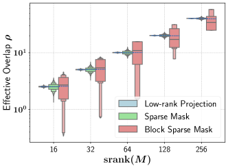
(a) Log-scaled boxen plot of distribution of $\rho$

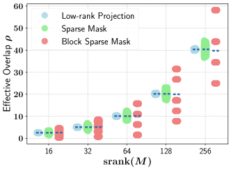
(b) Strip plot of distribution of $\rho$

Figure 4: Alternative visualizations of the effective overlap $\rho$ in Figure 2. (a) The log-scaled boxen plot provides better visibility of the distribution of small $\mathrm{srank}(\mathbf{M})$, capturing variations that are otherwise compressed in the linear scale. (b) The strip plot uncover the discrete nature of the block sparse masking ,which deviates from the continuous assumption underlying the boxen plot.

F.2 Loss Curves for Different $M$ Across Varying $\bar{\rho}$

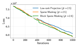
(a) $\mathrm{srank}(M)=16$

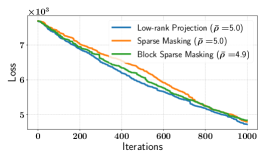
(b) $\mathrm{srank}(M)=32$

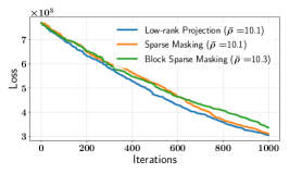
(c) $\mathrm{srank}(M)=64$

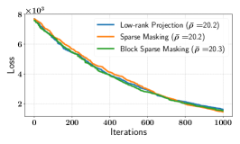
(d) $\mathrm{srank}(M)=128$

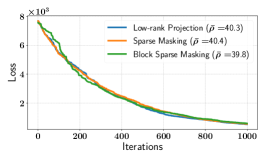
(e) $\mathrm{srank}(M)=256$

Figure 5: Loss curves for different methods under varying $\mathrm{srank}(\mathbf{M})$. The convergence behavior remains similar across all three methods, corroborating the observation from Figure 2 that the mean effective overlap $\bar{\rho}$ are nearly identical. This suggests that in purely random substructure scenarios, different methods exhibit comparable convergence dynamics despite their structural differences. $\eta=10^{-4}$ is used for the experiments.

References

- Ahn & Cutkosky (2024) Ahn, K. and Cutkosky, A. Adam with model exponential moving average is effective for nonconvex optimization. In The Thirty-eighth Annual Conference on Neural Information Processing Systems, 2024. URL https://openreview.net/forum?id=v416YLOQuU.
- Bar-Haim et al. (2006) Bar-Haim, R., Dagan, I., Dolan, B., Ferro, L., Giampiccolo, D., Magnini, B., and Szpektor, I. The second pascal recognising textual entailment challenge. In Proceedings of the second PASCAL challenges workshop on recognising textual entailment, volume 1. Citeseer, 2006.
- Bentivogli et al. (2009) Bentivogli, L., Clark, P., Dagan, I., and Giampiccolo, D. The fifth pascal recognizing textual entailment challenge. TAC, 7(8):1, 2009.
- Berahas et al. (2022) Berahas, A. S., Cao, L., Choromanski, K., and Scheinberg, K. A theoretical and empirical comparison of gradient approximations in derivative-free optimization. Foundations of Computational Mathematics, 22(2):507–560, 2022.
- Bousquet & Elisseeff (2002) Bousquet, O. and Elisseeff, A. Stability and generalization. The Journal of Machine Learning Research, 2:499–526, 2002.
- Cai et al. (2021) Cai, H., Lou, Y., McKenzie, D., and Yin, W. A zeroth-order block coordinate descent algorithm for huge-scale black-box optimization. In International Conference on Machine Learning, pp. 1193–1203. PMLR, 2021.
- Chen et al. (2017) Chen, P.-Y., Zhang, H., Sharma, Y., Yi, J., and Hsieh, C.-J. Zoo: Zeroth order optimization based black-box attacks to deep neural networks without training substitute models. In Proceedings of the 10th ACM workshop on artificial intelligence and security, pp. 15–26, 2017.
- Chen et al. (2019a) Chen, X., Liu, S., Sun, R., and Hong, M. On the convergence of a class of adam-type algorithms for non-convex optimization. In International Conference on Learning Representations, 2019a. URL https://openreview.net/forum?id=H1x-x309tm.
- Chen et al. (2019b) Chen, X., Liu, S., Xu, K., Li, X., Lin, X., Hong, M., and Cox, D. Zo-adamm: Zeroth-order adaptive momentum method for black-box optimization. Advances in neural information processing systems, 32, 2019b.
- Chen et al. (2024) Chen, Y., Zhang, Y., Cao, L., Yuan, K., and Wen, Z. Enhancing zeroth-order fine-tuning for language models with low-rank structures. arXiv preprint arXiv:2410.07698, 2024.
- Cheng et al. (2021) Cheng, S., Wu, G., and Zhu, J. On the convergence of prior-guided zeroth-order optimization algorithms. Advances in Neural Information Processing Systems, 34:14620–14631, 2021.
- Clark et al. (2019) Clark, C., Lee, K., Chang, M.-W., Kwiatkowski, T., Collins, M., and Toutanova, K. Boolq: Exploring the surprising difficulty of natural yes/no questions. In Proceedings of the 2019 Conference of the North American Chapter of the Association for Computational Linguistics: Human Language Technologies, Volume 1 (Long and Short Papers), pp. 2924–2936, 2019.
- Collobert (2004) Collobert, R. Large scale machine learning. Technical report, Université de Paris VI, 2004.
- Dagan et al. (2005) Dagan, I., Glickman, O., and Magnini, B. The pascal recognising textual entailment challenge. In Machine learning challenges workshop, pp. 177–190. Springer, 2005.
- Davis et al. (2022) Davis, D., Drusvyatskiy, D., Lee, Y. T., Padmanabhan, S., and Ye, G. A gradient sampling method with complexity guarantees for lipschitz functions in high and low dimensions. Advances in neural information processing systems, 35:6692–6703, 2022.
- De Marneffe et al. (2019) De Marneffe, M.-C., Simons, M., and Tonhauser, J. The commitmentbank: Investigating projection in naturally occurring discourse. In proceedings of Sinn und Bedeutung, volume 23, pp. 107–124, 2019.
- Dua et al. (2019) Dua, D., Wang, Y., Dasigi, P., Stanovsky, G., Singh, S., and Gardner, M. Drop: A reading comprehension benchmark requiring discrete reasoning over paragraphs. In Proceedings of the 2019 Conference of the North American Chapter of the Association for Computational Linguistics: Human Language Technologies, Volume 1 (Long and Short Papers), pp. 2368–2378, 2019.
- Duchi et al. (2015) Duchi, J. C., Jordan, M. I., Wainwright, M. J., and Wibisono, A. Optimal rates for zero-order convex optimization: The power of two function evaluations. IEEE Transactions on Information Theory, 61(5):2788–2806, 2015.
- Gautam et al. (2024) Gautam, T., Park, Y., Zhou, H., Raman, P., and Ha, W. Variance-reduced zeroth-order methods for fine-tuning language models. In Forty-first International Conference on Machine Learning, 2024. URL https://openreview.net/forum?id=VHO4nE7v41.
- Ghadimi & Lan (2013) Ghadimi, S. and Lan, G. Stochastic first-and zeroth-order methods for nonconvex stochastic programming. SIAM journal on optimization, 23(4):2341–2368, 2013.
- Giampiccolo et al. (2007) Giampiccolo, D., Magnini, B., Dagan, I., and Dolan, W. B. The third pascal recognizing textual entailment challenge. In Proceedings of the ACL-PASCAL workshop on textual entailment and paraphrasing, pp. 1–9, 2007.
- Guo et al. (2024) Guo, W., Long, J., Zeng, Y., Liu, Z., Yang, X., Ran, Y., Gardner, J. R., Bastani, O., De Sa, C., Yu, X., et al. Zeroth-order fine-tuning of llms with extreme sparsity. arXiv preprint arXiv:2406.02913, 2024.
- Hanson & Wright (1971) Hanson, D. L. and Wright, F. T. A bound on tail probabilities for quadratic forms in independent random variables. The Annals of Mathematical Statistics, 42(3):1079–1083, 1971.
- Hardt et al. (2016) Hardt, M., Recht, B., and Singer, Y. Train faster, generalize better: Stability of stochastic gradient descent. In International conference on machine learning, pp. 1225–1234. PMLR, 2016.
- Ipsen & Saibaba (2024) Ipsen, I. C. and Saibaba, A. K. Stable rank and intrinsic dimension of real and complex matrices. arXiv preprint arXiv:2407.21594, 2024.
- Isserlis (1918) Isserlis, L. On a formula for the product-moment coefficient of any order of a normal frequency distribution in any number of variables. Biometrika, 12(1/2):134–139, 1918.
- Ji et al. (2019) Ji, K., Wang, Z., Zhou, Y., and Liang, Y. Improved zeroth-order variance reduced algorithms and analysis for nonconvex optimization. In International conference on machine learning, pp. 3100–3109. PMLR, 2019.
- Khashabi et al. (2018) Khashabi, D., Chaturvedi, S., Roth, M., Upadhyay, S., and Roth, D. Looking beyond the surface: A challenge set for reading comprehension over multiple sentences. In Proceedings of the 2018 Conference of the North American Chapter of the Association for Computational Linguistics: Human Language Technologies, Volume 1 (Long Papers), pp. 252–262, 2018.
- Kingma & Ba (2015) Kingma, D. and Ba, J. Adam: A method for stochastic optimization. In International Conference on Learning Representations (ICLR), San Diega, CA, USA, 2015.
- Kornowski & Shamir (2024) Kornowski, G. and Shamir, O. An algorithm with optimal dimension-dependence for zero-order nonsmooth nonconvex stochastic optimization. Journal of Machine Learning Research, 25(122):1–14, 2024.
- Kurakin et al. (2017) Kurakin, A., Goodfellow, I. J., and Bengio, S. Adversarial machine learning at scale. In International Conference on Learning Representations, 2017. URL https://openreview.net/forum?id=BJm4T4Kgx.
- Lei (2023) Lei, Y. Stability and generalization of stochastic optimization with nonconvex and nonsmooth problems. In The Thirty Sixth Annual Conference on Learning Theory, pp. 191–227. PMLR, 2023.
- Levesque et al. (2012) Levesque, H., Davis, E., and Morgenstern, L. The winograd schema challenge. In Thirteenth international conference on the principles of knowledge representation and reasoning, 2012.
- Li et al. (2021) Li, Y., Ren, X., Zhao, F., and Yang, S. A zeroth-order adaptive learning rate method to reduce cost of hyperparameter tuning for deep learning. Applied Sciences, 11(21):10184, 2021.
- Liu et al. (2018) Liu, S., Kailkhura, B., Chen, P.-Y., Ting, P., Chang, S., and Amini, L. Zeroth-order stochastic variance reduction for nonconvex optimization. Advances in Neural Information Processing Systems, 31, 2018.
- Liu et al. (2024a) Liu, X., Zhang, H., Gu, B., and Chen, H. General stability analysis for zeroth-order optimization algorithms. In The Twelfth International Conference on Learning Representations, 2024a. URL https://openreview.net/forum?id=AfhNyr73Ma.
- Liu et al. (2024b) Liu, Y., Zhu, Z., Gong, C., Cheng, M., Hsieh, C.-J., and You, Y. Sparse mezo: Less parameters for better performance in zeroth-order llm fine-tuning. arXiv preprint arXiv:2402.15751, 2024b.
- Luo et al. (2024) Luo, Q., Yu, H., and Li, X. Badam: A memory efficient full parameter training method for large language models. arXiv preprint arXiv:2404.02827, 2024.
- Magnus et al. (1978) Magnus, J. R. et al. The moments of products of quadratic forms in normal variables. Univ., Instituut voor Actuariaat en Econometrie, 1978.
- Malladi et al. (2023) Malladi, S., Gao, T., Nichani, E., Damian, A., Lee, J. D., Chen, D., and Arora, S. Fine-tuning language models with just forward passes. Advances in Neural Information Processing Systems, 36:53038–53075, 2023.
- Nesterov & Spokoiny (2017) Nesterov, Y. and Spokoiny, V. Random gradient-free minimization of convex functions. Foundations of Computational Mathematics, 17(2):527–566, 2017.
- Papernot et al. (2017) Papernot, N., McDaniel, P., Goodfellow, I., Jha, S., Celik, Z. B., and Swami, A. Practical black-box attacks against machine learning. In 2017 ACM Asia Conference on Computer and Communications Security, ASIA CCS 2017, pp. 506–519. Association for Computing Machinery, Inc, 2017.
- Park et al. (2024) Park, S., Yun, J., Kim, S.-Y., Yang, J. Y., Jung, Y., Kundu, S., Kim, K., and Yang, E. MeZO-a$^{3}$dam: Memory-efficient zeroth-order adam with adaptivity adjustments for fine-tuning LLMs, 2024. URL https://openreview.net/forum?id=OBIuFjZzmp.
- Pilehvar & Camacho-Collados (2018) Pilehvar, M. T. and Camacho-Collados, J. Wic: the word-in-context dataset for evaluating context-sensitive meaning representations. arXiv preprint arXiv:1808.09121, 2018.
- Rajpurkar et al. (2018) Rajpurkar, P., Jia, R., and Liang, P. Know what you don’t know: Unanswerable questions for squad. In Proceedings of the 56th Annual Meeting of the Association for Computational Linguistics (Volume 2: Short Papers), pp. 784–789, 2018.
- Rando et al. (2023) Rando, M., Molinari, C., Rosasco, L., and Villa, S. An optimal structured zeroth-order algorithm for non-smooth optimization. In Thirty-seventh Conference on Neural Information Processing Systems, 2023. URL https://openreview.net/forum?id=SfdkS6tt81.
- Reddi et al. (2018) Reddi, S. J., Kale, S., and Kumar, S. On the convergence of adam and beyond. In International Conference on Learning Representations, 2018. URL https://openreview.net/forum?id=ryQu7f-RZ.
- Robbins & Monro (1951) Robbins, H. and Monro, S. A Stochastic Approximation Method. The Annals of Mathematical Statistics, 22(3):400 – 407, 1951. doi: 10.1214/aoms/1177729586. URL https://doi.org/10.1214/aoms/1177729586.
- Roemmele et al. (2011) Roemmele, M., Bejan, C. A., and Gordon, A. S. Choice of plausible alternatives: An evaluation of commonsense causal reasoning. In 2011 AAAI spring symposium series, 2011.
- Shamir (2013) Shamir, O. On the complexity of bandit and derivative-free stochastic convex optimization. In Conference on Learning Theory, pp. 3–24. PMLR, 2013.
- Socher et al. (2013) Socher, R., Perelygin, A., Wu, J., Chuang, J., Manning, C. D., Ng, A., and Potts, C. Recursive deep models for semantic compositionality over a sentiment treebank. In Yarowsky, D., Baldwin, T., Korhonen, A., Livescu, K., and Bethard, S. (eds.), Proceedings of the 2013 Conference on Empirical Methods in Natural Language Processing, pp. 1631–1642, Seattle, Washington, USA, October 2013. Association for Computational Linguistics. URL https://aclanthology.org/D13-1170.
- Spall (1992) Spall, J. C. Multivariate stochastic approximation using a simultaneous perturbation gradient approximation. IEEE transactions on automatic control, 37(3):332–341, 1992.
- Sun & Ye (2021) Sun, R. and Ye, Y. Worst-case complexity of cyclic coordinate descent: O (nˆ 2) o (n 2) gap with randomized version. Mathematical Programming, 185:487–520, 2021.
- Wang et al. (2019) Wang, A., Pruksachatkun, Y., Nangia, N., Singh, A., Michael, J., Hill, F., Levy, O., and Bowman, S. R. SuperGLUE: A stickier benchmark for general-purpose language understanding systems. arXiv preprint 1905.00537, 2019.
- Wang et al. (2022) Wang, X., Guo, W., Su, J., Yang, X., and Yan, J. Zarts: On zero-order optimization for neural architecture search. Advances in Neural Information Processing Systems, 35:12868–12880, 2022.
- Wick (1950) Wick, G.-C. The evaluation of the collision matrix. Physical review, 80(2):268, 1950.
- Wright (1973) Wright, F. T. A bound on tail probabilities for quadratic forms in independent random variables whose distributions are not necessarily symmetric. The Annals of Probability, 1(6):1068–1070, 1973.
- Yu et al. (2024) Yu, Z., Zhou, P., Wang, S., Li, J., and Huang, H. Subzero: Random subspace zeroth-order optimization for memory-efficient llm fine-tuning. arXiv preprint arXiv:2410.08989, 2024.
- Yun et al. (2022) Yun, J., Lozano, A., and Yang, E. Adablock: Sgd with practical block diagonal matrix adaptation for deep learning. In International Conference on Artificial Intelligence and Statistics, pp. 2574–2606. PMLR, 2022.
- Zhang et al. (2020) Zhang, J., Lin, H., Jegelka, S., Sra, S., and Jadbabaie, A. Complexity of finding stationary points of nonconvex nonsmooth functions. In International Conference on Machine Learning, pp. 11173–11182. PMLR, 2020.
- Zhang et al. (2024a) Zhang, P., Liu, Y., Zhou, Y., Du, X., Wei, X., Wang, T., and Chen, M. When foresight pruning meets zeroth-order optimization: Efficient federated learning for low-memory devices. arXiv preprint arXiv:2405.04765, 2024a.
- Zhang et al. (2018) Zhang, S., Liu, X., Liu, J., Gao, J., Duh, K., and Van Durme, B. Record: Bridging the gap between human and machine commonsense reading comprehension. arXiv preprint arXiv:1810.12885, 2018.
- Zhang et al. (2022a) Zhang, S., Roller, S., Goyal, N., Artetxe, M., Chen, M., Chen, S., Dewan, C., Diab, M., Li, X., Lin, X. V., et al. Opt: Open pre-trained transformer language models. arXiv preprint arXiv:2205.01068, 2022a.
- Zhang et al. (2022b) Zhang, Y., Yao, Y., Jia, J., Yi, J., Hong, M., Chang, S., and Liu, S. How to robustify black-box ML models? a zeroth-order optimization perspective. In International Conference on Learning Representations, 2022b. URL https://openreview.net/forum?id=W9G_ImpHlQd.
- Zhang et al. (2024b) Zhang, Y., Chen, C., Ding, T., Li, Z., Sun, R., and Luo, Z.-Q. Why transformers need adam: A hessian perspective. arXiv preprint arXiv:2402.16788, 2024b.
- Zhang et al. (2024c) Zhang, Y., Chen, C., Li, Z., Ding, T., Wu, C., Ye, Y., Luo, Z.-Q., and Sun, R. Adam-mini: Use fewer learning rates to gain more. arXiv preprint arXiv:2406.16793, 2024c.
- Zhang et al. (2024d) Zhang, Y., Li, P., Hong, J., Li, J., Zhang, Y., Zheng, W., Chen, P.-Y., Lee, J. D., Yin, W., Hong, M., Wang, Z., Liu, S., and Chen, T. Revisiting zeroth-order optimization for memory-efficient LLM fine-tuning: A benchmark. In Salakhutdinov, R., Kolter, Z., Heller, K., Weller, A., Oliver, N., Scarlett, J., and Berkenkamp, F. (eds.), Proceedings of the 41st International Conference on Machine Learning, volume 235 of Proceedings of Machine Learning Research, pp. 59173–59190. PMLR, 21–27 Jul 2024d. URL https://proceedings.mlr.press/v235/zhang24ad.html.