MotionPCM: Real-Time Motion Synthesis with Phased Consistency Model
Abstract
Diffusion models have become a popular choice for human motion synthesis due to their powerful generative capabilities. However, their high computational complexity and large sampling steps pose challenges for real-time applications. Fortunately, the Consistency Model (CM) provides a solution to greatly reduce the number of sampling steps from hundreds to a few, typically fewer than four, significantly accelerating the synthesis of diffusion models. However, its application to text-conditioned human motion synthesis in latent space remains challenging. In this paper, we introduce MotionPCM, a phased consistency model-based approach designed to improve the quality and efficiency of real-time motion synthesis in latent space.
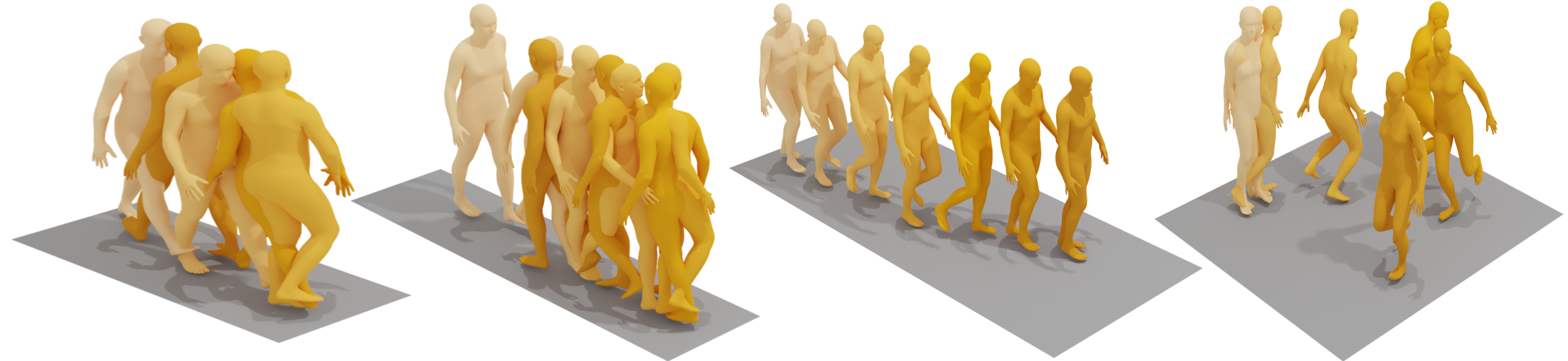
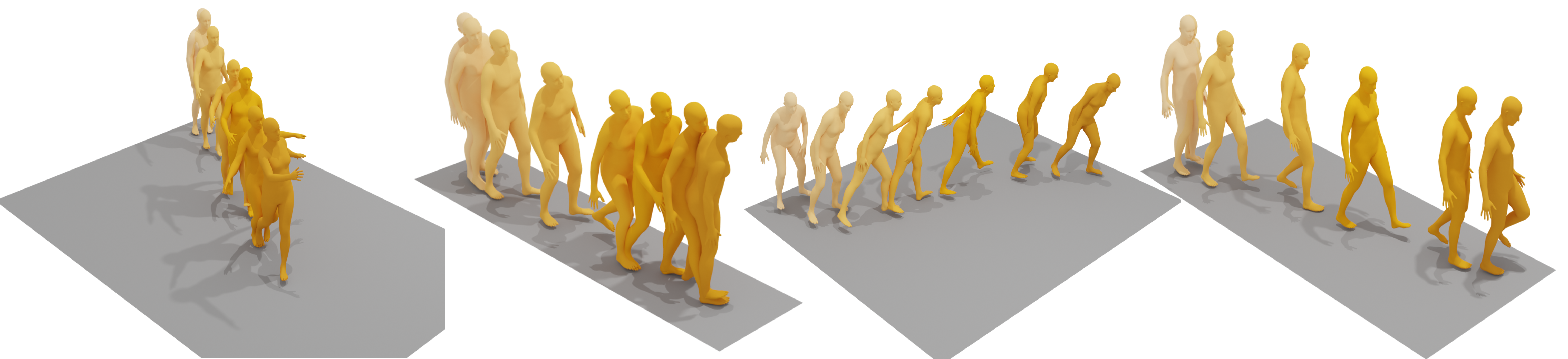
![[Uncaptioned image]](/html/2501.19083/assets/sec/figs/sample_0.png)
1 Introduction
Driven by the development of multimodal, human motion synthesis has become capable of responding accordingly with different conditional inputs, including text Lin et al. (2018); Zhang et al. (2022), action categories Tevet et al. (2023); Chen et al. (2023), action sequence Dai et al. (2025) and music Li et al. (2021). These developments can bring immense potentials in areas, such as game industry, film production and virtual reality.
MotionDiffuse Zhang et al. (2022) is the first work to apply the diffusion model to generate human motion, achieving remarkable performance. However, MotionDiffuse processes the entire motion sequence with the diffusion model, leading to high computational resource demands and significant time consumption. To alleviate these issues, MLD Chen et al. (2023) utilising a Variational Autoencoder (VAE) Kingma (2013) to compress the motion sequence into latent codes before sending them to the diffusion model. This approach greatly boosts the speed and quality of motion synthesis but still requires tens of inference steps with the help of DDIM Song et al. (2020a), making it impractical to implement motion synthesis in real time.
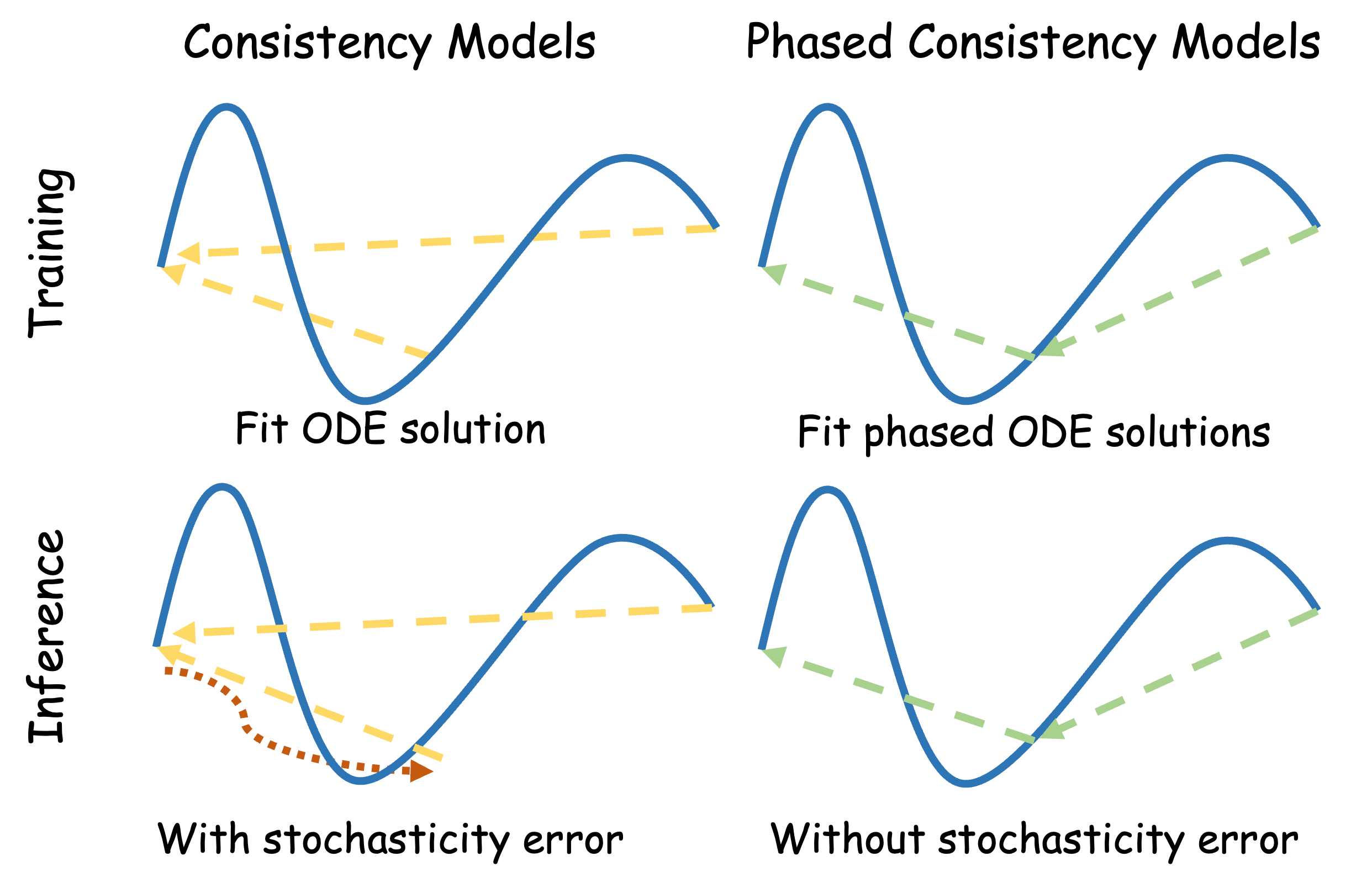
Building upon MLD, MotionLCM Dai et al. (2025) utilise the Latent Consistency Model (LCM) Luo et al. (2023), enabling few-step inference and thus achieving real-time motion synthesis with a diffusion model. However, LCM’s design suffers from several issues, including consistency issues caused by accumulated stochastic noise during multi-step sampling as shown in Figure 2. In addition, LCM suffers from significantly degraded sample quality in low-step settings. Identifying these flaws of LCM, Phased Consistency Model (PCM) Wang et al. (2024) introduces a refined architecture to address these limitations. Taking Figure 2 as an example, PCM is trained with two sub-trajectories, enabling efficient 2-step deterministic sampling without introducing stochastic noise. Experimental results on image generation tasks demonstrate that PCM outperforms LCM in different step generation settings. Nevertheless, the performance of PCM on human motion generation tasks remains unexplored.
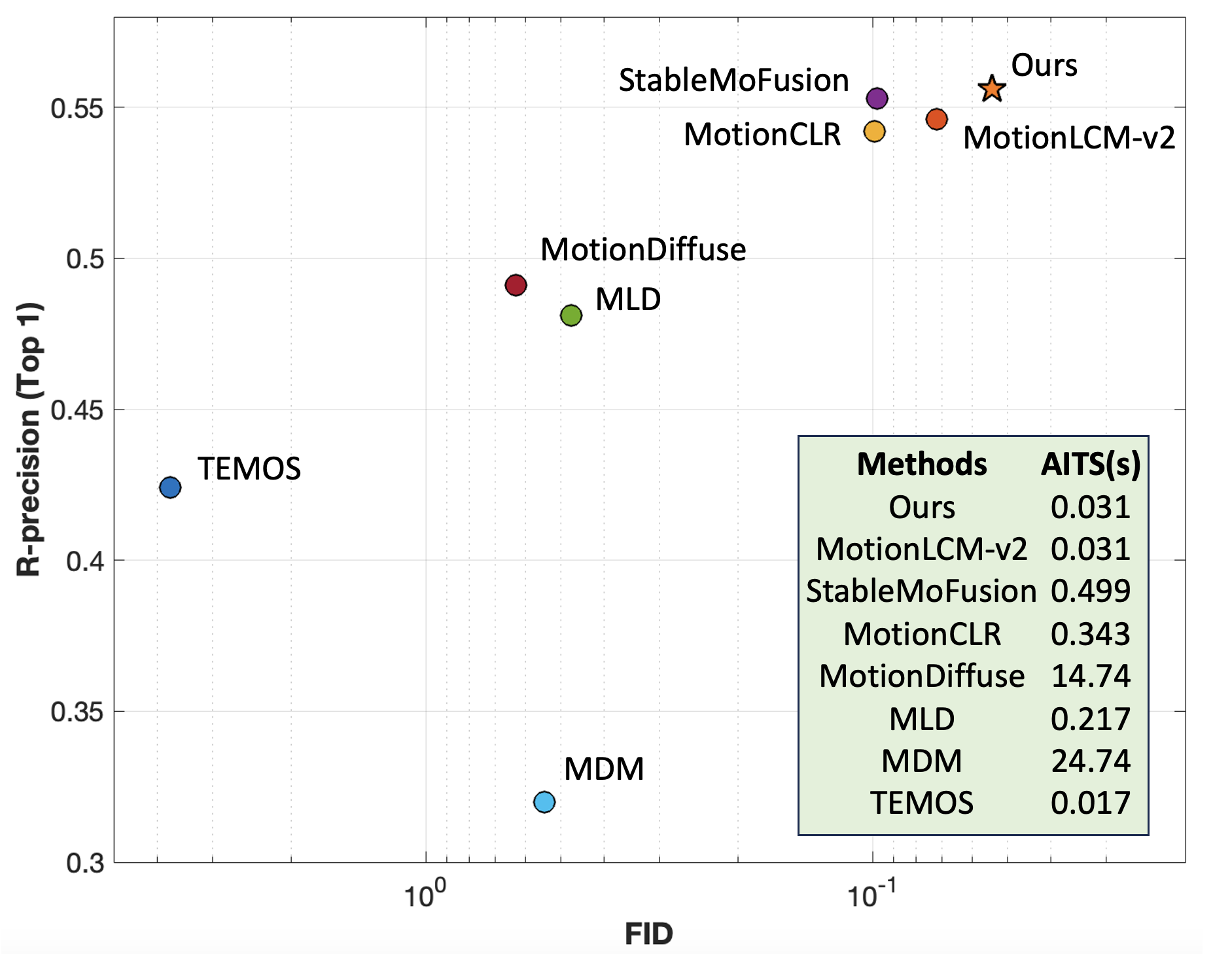
In this paper, we incorporate PCM into the motion synthesis pipeline and propose a new motion synthesis approach, MotionPCM, allowing real-time motion synthesis with improved generation quality (see Figure 3). Similar to MotionLCM, our model is distilled from MLD, but differently, we split the entire trajectory into N segments where N corresponds to the number of inference steps. Instead of forcing all points in the trajectory to the original, we only map points in a certain interval to the start of that interval, ensuring consistent predictions for the start of the interval across different points within it. This design allows us to achieve N-step sampling deterministically, avoiding the accumulation of stochastic errors. Furthermore, inspired by PCM and CTM Kim et al. (2023), we employ an additional discriminator to provide extra supervision, enhancing performance in low-step settings.
We summarise our main contributions as follows:
-
•
Leveraging the multi-interval design of PCM, we propose MotionPCM, an improved pipeline for real-time motion synthesis.
-
•
Introducing an additional discriminator for extra supervision significantly enhances the quality of motion synthesis.
-
•
Experiments on a large-scale public dataset demonstrate that our approach achieves the state-of-the-art performance in terms of speed and generation performance, with efficient sampling requiring fewer than four steps.
2 Related Work
2.1 Motion Synthesis
Motion synthesis seeks to generate human motion under various conditions to support a wide range of applications Zhang et al. (2022, 2023a); Ghosh et al. (2021). The evolution of motion synthesis models has mirrored advances in machine learning, moving from deterministic methods with limited variability towards generative approaches—such as VAEs and GANs Xia et al. (2015); Kingma (2013); Goodfellow et al. (2020)—and more recently, diffusion models, which have further transformed the field by utilising noise-based iterative refinement Zhang et al. (2022); Tevet et al. (2023).
Among the earliest works to adopt diffusion models for motion generation is Zhang et al. (2022). By capitalising on the advantages of diffusion models in probabilistic mapping and realistic synthesis, it demonstrates that diffusion-based methods can outperform earlier approaches, particularly in conditional generation scenarios (e.g., text-driven or action-conditioned). Nevertheless, human motions exhibit high diversity and often differ significantly in distribution from their conditional modalities, making it challenging to learn a robust probabilistic mapping from such modalities to human motion sequences Chen et al. (2023). Furthermore, raw motion capture data can be redundant and noisy. To mitigate these issues, subsequent research—exemplified by the Motion Latent-based Diffusion model (MLD) Chen et al. (2023) uses a VAE to produce representative, low-dimensional latent codes from the motion sequence and perform the diffusion process within that latent space.
While latent-space diffusion mitigates some of the aforementioned challenges, efficiency remains a critical bottleneck due to the computational cost of multi-step sampling. To overcome this, inspired by consistency models Song et al. (2023); Luo et al. (2023), MotionLCM Dai et al. (2025)) takes MLD as the teacher model to distill the model so that motion generation can be achieved in a low sampling step. It also incorporates an explicit control network to control the motion generation based on the given motion sequence. Besides, identifying some drawbacks of the VAE design of MLD, MotionLCM-v2 Dai et al. (2024) further improves VAE network by introducing a trainable linear layer after the VAE latent tokens to strengthen multimodal signal modulation, while removing unnecessary ReLU activations to preserve negative components in text features, thereby achieving further performance gains.
2.2 Acceleration of Diffusion Models
Since the advent of Denoising Diffusion Probabilistic Models (DDPMs) Ho et al. (2020), researchers have been striving to overcome the limitations of sequential sampling by achieving a more favourable balance between quality and speed. A key advance came with Denoising Diffusion Implicit Models (DDIMs) Song et al. (2020a), which transform DDPM’s stochastic diffusion process into a deterministic one, eliminating the randomness of Markov chains and introducing the possibility of skip sampling to accelerate generation. Subsequently, Consistency Models (CMs) Song et al. (2023) take a further step by imposing a consistency constraint that directly maps noisy inputs to clean outputs without iterative denoising, enabling single-step generation and substantially improving speed.
Latent Consistency Model (LCM) Luo et al. (2023) builds on CMs by operating in a latent space, unlike CMs, which work in the pixel domain. This approach enables LCM to handle more challenging tasks, such as text-to-image generation, with improved efficiency. As a result, LCM can serve as a foundational component to accelerate latent diffusion models, which has been employed in motion synthesis like MotionLCM Dai et al. (2025). However, it still faces limitations—particularly in balancing efficiency, consistency, and controllability with varying inference steps, thereby leaving room for further refinement. Analysing the reasons behind these challenges, Phased Consistency Model (PCM) Wang et al. (2024)) partitions the ODE path into multiple sub-paths and enforce consistency within each sub-path. Additionally, PCM incorporates an adversarial loss, further improving the quality of image generation. In this paper, we apply PCM to the domain of motion synthesis and propose a new method, MotionPCM, for generating high-quality motion sequences in real time.
3 Preliminaries
Given , the data distribution, a traceable diffusion process defined by is normally used to transform to , a prior distribution. Equivalently, score-based diffusion models Song et al. (2020b) define a continuous Stochastic Differential Equation (SDE) as the diffusion process:
| (1) |
where is the standard -dimensional Wiener process, is a -valued function and is a scalar function. The reverse-time SDE transforms the prior distribution back to the original data distribution. It is expressed as:
| (2) |
where is again the standard -dimensional Wiener process in the reversed process, represents the probability density function of at time . To estimate score , a score-based model is trained to approximate as much as possible.
There exists a deterministic reversed-time trajectory Song et al. (2020b), satisfying an ODE, known as the probability flow ODE (PF-ODE):
| (3) |
Rather than using to predict the score, consistency models Song et al. (2023) directly learn a function to predict the solution of PF-ODE by mapping any points in the ODE trajectory to the origin of this trajectory, , where is a fixed small positive number. Formally, for all , it holds that:
| (4) |
However, for multi-step sampling, CM will introduce random noise at each step since generating intermediate states along the sampling trajectory involves reintroducing noise, which accumulates and causes inconsistencies in the final output. To address this issue, PCM Wang et al. (2024) splits the solution trajectory of PF-ODE into multiple sub-intervals with M+1 edge timesteps , , …, , where and . Each sub-trajectory is treated as an independent CM, with a consistency function defined as: for all
| (5) |
Lu et al. (2022) shows an exact solution from timestep to for PF-ODE:
| (6) |
where and is an inverse function with . Using an epsilon (noise) prediction network , this solution can be approximated as:
| (7) |
The solution needs to know the noise predictions throughout the entire interval between time and , while consistency models can only access to for a single inference. To address this, Wang et al. (2024) parameterises as follows:
| (8) |
To satisfy the boundary condition of each sub-trajectory of the PCM, i.e., , a parameterised form below is typically employed:
| (9) |
where gradually increases to 1 and progressively decays to 0 as decreases over the time interval from to . In fact, in Eq. (8), the boundary condition is inherently satisfied, and as a result, the simplified form shown below can be used directly:
| (10) |
4 Method
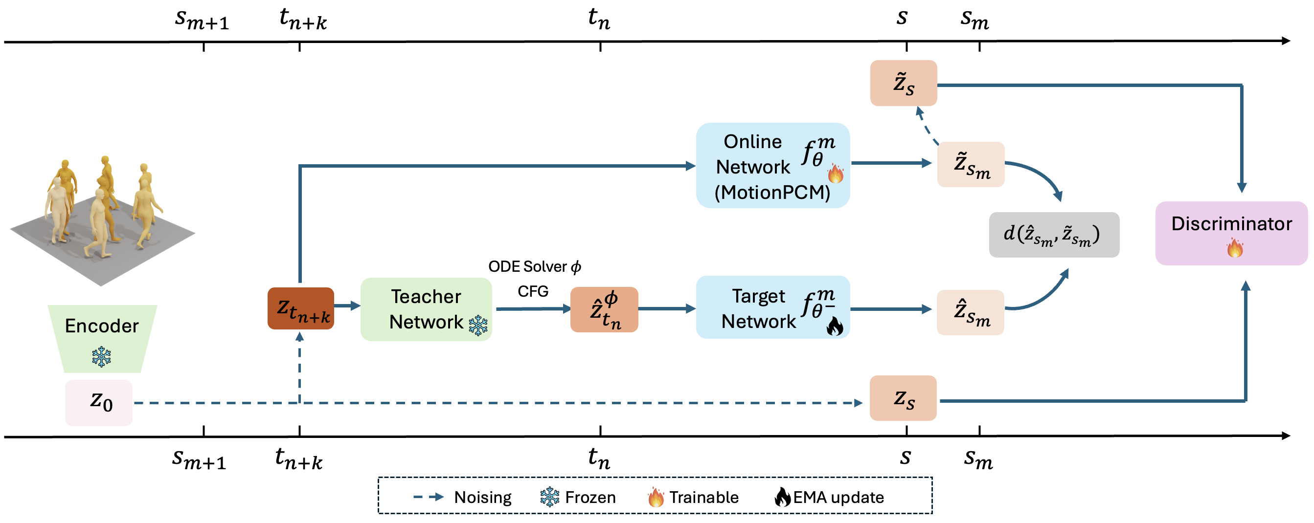
As shown in Figure 4, we introduce MotionPCM, a novel framework for real-time motion synthesis. To provide a clear understanding of our method, we divide our method into four main segments. Section 4.1 explains the use of a Variational Autoencoder (VAE) and latent diffusion model as pre-training models to initialise the framework. Section 4.2 describes the integration of the phased consistency model within the motion synthesis pipeline. Section 4.3 details the design and role of the discriminator, which provides adversarial loss to enforce distribution consistency while improving overall performance. Section 4.4 illustrates the process of generating motion sequences from a prior distribution using PCM during inference.
4.1 VAE and Latent Diffusion Model for Motion Data Pre-training
Following the two-stage training approach of MLD Chen et al. (2023), we first employ a VAE Kingma (2013) to compress motion sequences into a lower-dimensional latent space. More specifically, the encoder maps motion sequences , where is the frame length and is the number of features, to a latent code where and are much smaller than and . Then a decoder is used to reconstruct the motion sequence . This process significantly reduces the dimensionality of the motion data, accelerating latent diffusion training in the second stage. Building upon this, MotionLCM-V2 Dai et al. (2024) introduces an improved VAE to enhance the representation quality of motion data. In our work, we adopt the improved VAE proposed by MotionLCM-V2 as the backbone.
In the second stage, we train a latent diffusion model in the latent space of this enhanced VAE, following MLD. Here, the latent diffusion model is an epsilon prediction network. Readers are referred to Chen et al. (2023) for more details. This trained diffusion model will be used as the teacher network to guide the distillation process in our work.
4.2 Accelerating Motion Synthesis via PCM
Definition. Following the definition of PCM Wang et al. (2024), we split our solution trajectory in the latent space into sub-trajectories, with edge timestep where and . In each sub-time interval , the consistency function is defined as Eq. (5). We train in Eq. (10) to estimate , applying consistency constraint on each sub-trajectory, i.e., for all and .
PCM Consistency distillation. Once we obtain the pre-trained VAEs and latent diffusion model from Section 4.1, we can get the meaningful latent code from VAE and use this latent diffusion model as our frozen teacher network to distill our MotionPCM model, i.e., online network in Figure 4. Following Dai et al. (2025), online network () is initialised from the teacher network with trainable weights , while the target network () is also initialised from the teacher network but updated using Exponential Moving Average (EMA) of the online network’s parameters. We obtain by applying forward diffusion with steps to , positioning it within the time interval .
This work focuses on text-conditioned motion generation where Classifier-free Guidance (CFG) Ho and Salimans (2022) has been used frequently to align conditions in diffusion models. Following previous works Chen et al. (2023); Dai et al. (2025); Luo et al. (2023), we also employ CFG in our framework. To distinguish used in consistency model, we use to represent the diffusion model, which corresponds to our teacher network. It can be express as:
| (11) |
where denotes text condition, the guidance scale is uniformly sampled from , and indicates an empty condition (i.e., a blank text input). is then estimated from by performing k-step skip using , followed by an ODE solver , such as DDIM Song et al. (2020a). To efficiently perform the guided distillation, Dai et al. (2025); Luo et al. (2023) add into an augmented consistency function . Similarly, in our work, we extend our phased consistency function to .
Following CMs Song et al. (2023); Wang et al. (2024), the phased consistency distillation loss is then defined as follows:
| (12) |
where is Huber loss Huber (1992) in our implementation. The online network’s parameters are updated by minimising through the standard gradient descent algorithms, such as AdamW Loshchilov (2017). Meanwhile, as mentioned earlier, the target network’s parameters, is updated in EMA fashion: .
4.3 Discriminator
Building on the work of Kim et al. (2023); Wang et al. (2024), which demonstrated that incorporating an adversarial loss from a discriminator can enhance the image generation quality of diffusion models in few-step sampling settings, we integrate an additional discriminator with adversarial loss into our motion synthesis pipeline.
A pair of and is sent to the discriminator as illustrated in Figure 4. More specifically, we first compute the solutions and through the online network and target network, respectively. Following Wang et al. (2024), noise is added to , producing for . However, unlike Wang et al. (2024), where is used to produce , we derive from directly since Kim et al. (2023) highlights that leveraging direct training signals from data label is a key to achieve optimal performance. Inspired by Wang et al. (2024), we then apply an adversarial loss as follows:
| (13) |
where is a discriminator, ReLU is an non-linear activation function. The loss is optimised using a min-max strategy Goodfellow et al. (2020).
The total loss combining phased consistency distillation loss and adversarial loss is expressed as:
| (14) |
where is a hyper-parameter.
4.4 Inference
During inference, we sample from a prior distribution, such as standard normal distribution . Based on the transition map defined in Wang et al. (2024): which transform any point on -th sub-trajectory to the solution point of -th trajectory, we can get the solution estimation . Finally, the human motion sequence is generated through the decoder .
5 Numerical Experiments
Dataset. We base our experiments on the widely used HumanML3D dataset Guo et al. (2022a), which comprises 14,616 distinct human motion sequences accompanied by 44,970 textual annotations. In line with previous studies Dai et al. (2025); Chen et al. (2023); Guo et al. (2022a), we employ a redundant motion representation that includes root velocity, root height, local joint positions, velocities, root-space rotations, and foot-contact binary indicators to ensure a fair comparison across methods.
| Methods | AITS | R-Precision | FID | MM Dist | Diversity | MModality | ||
|---|---|---|---|---|---|---|---|---|
| Top 1 | Top 2 | Top 3 | ||||||
| Real | - | - | ||||||
| Seq2Seq Lin et al. (2018) | - | - | ||||||
| JL2P Ahuja and Morency (2019) | - | - | ||||||
| T2G Bhattacharya et al. (2021) | - | - | ||||||
| Hier Ghosh et al. (2021) | - | - | ||||||
| T2M Guo et al. (2022a) | ||||||||
| TM2T Guo et al. (2022b) | ||||||||
| MotionDiffuse Zhang et al. (2022) | ||||||||
| MDM Tevet et al. (2023) | ||||||||
| MLD Chen et al. (2023) | ||||||||
| T2M-GPT Zhang et al. (2023a) | ||||||||
| ReMoDiffuse Zhang et al. (2023b) | ||||||||
| MoMask Guo et al. (2024) | ||||||||
| StableMoFusion Huang et al. (2024) | ||||||||
| MotionCLR Chen et al. (2024) | ||||||||
| B2A-HDM Xie et al. (2024) | - | |||||||
| MotionLCM-V1 Dai et al. (2025) (1-step) | ||||||||
| MotionLCM-V1 Dai et al. (2025) (2-step) | ||||||||
| MotionLCM-V1 Dai et al. (2025) (4-step) | ||||||||
| MotionLCM-V2 Dai et al. (2024) (1-step) | 0.031 | |||||||
| MotionLCM-V2 Dai et al. (2024) (2-step) | ||||||||
| MotionLCM-V2 Dai et al. (2024) (4-step) | ||||||||
| Ours (1-step) | 0.031 | |||||||
| Ours (2-step) | 0.037 | |||||||
| Ours (4-step) | 0.046 | |||||||
Evaluation metrics. Following Guo et al. (2022a); Chen et al. (2023), we evaluate our model using the following metrics: (1) Average Inference Time per Sentence (AITS), which measures the time required to generate a motion sequence from a textual description, with lower values indicating faster inference; (2) R-Precision, capturing how accurately generated motions match their text prompts by checking whether the top-ranked motions align with the given descriptions, where higher scores indicate better accuracy; (3) Frechet Inception Distance (FID), assessing how closely the distribution of generated motions resembles real data, where lower scores indicate better quality; (4) Multimodal Distance (MM Dist), quantifying how well the motion features align with text features, with lower values signalling a tighter match between motions and prompts; (5) Diversity, which calculates variance through motion features to indicate the variety of generated motions across different samples; and (6) MultiModality (MModality), measuring generation diversity conditioned on the same text by evaluating how many distinct yet valid motions can be produced for a single prompt.
Implementation details. We conduct our experiments on a single NVIDIA RTX 6000 GPU with a batch size of 128 motion sequences fed into our model. The model is trained over 384K iterations using an AdamW Loshchilov (2017) optimiser with parameters , and an initial learning rate , which gradually decays following a cosine decay learning rate schedule. For the loss function, we set . The guidance scale ranges between , and and the Exponential Moving Average (EMA) rate is set as . Additionally, we use DDIM Song et al. (2020a) as our ODE solver and skip step .
5.1 Text-to-motion synthesis
| Real | MotionPCM (Ours) | MotionLCM-V2 | MLD |
|---|---|---|---|
| The rigs walk forward, then turn around, and continue walking before stopping where he started. | |||
 |
|||
| A person walks with a limp leg. | |||
 |
|||
| A man walks forward a few steps, raise his left hand to his face, then continue walking in a circle. | |||
 |
|||
In this section, we evaluate the performance of our proposed MotionPCM method on the text-to-motion task. We compare our approach with other baseline methods using the widely adopted HumanML3D dataset, conducting each experiment 20 times to establish results within a 95% confidence interval Dai et al. (2025); Guo et al. (2022a). Following previous studies Dai et al. (2025); Guo et al. (2022a), we employ the following evaluation metrics: Average Inference Time per Sentence (AITS), R-Precision, Frechet Inception Distance (FID), Multimodal Distance (MM Dist), Diversity, and MultiModality (MModality).
For benchmark comparisons, we select the most renowned and widely used models in the field. In particular, MotionLCM-v2 Dai et al. (2024), the improved version of MotionLCM-v1 Dai et al. (2025), is primarily compared with our method in different sampling steps. As illustrated in Table 1, our method achieves a sampling speed comparable to MotionLCM-v2 in terms of AITS while significantly outperforms it in R-Precision Top-1, Top-2 and Top-3, FID, and MM Dist across different sampling steps. Furthermore, our 4-step variant also outperforms the counterpart of MotionLCM-V2 in terms of Diversity while underperforming in MModality. These results demonstrate that our model is more superior than MotionLCM-V2 although both support real-time inference.
Compared to other approaches, the speed of our method surpasses most alternatives by a large margin, demonstrating its time efficiency. Our method with 1-step sampling can support motion synthesis over 30 frames per second, thereby making it possible for real-time applications. Regarding R-Precision, our method achieves the highest accuracy across Top-1, Top-2 and Top-3 metrics with our 2-step variants compared to other approaches. This consistent improvement highlights the reliability of MotionPCM in accurately aligning generated motions with textual descriptions. Similarly, in FID and MM Distance metrics, our method achieves the best scores with its 4-step and 2-step variants respectively. These results further highlight MotionPCM’s capability to generate high-quality and semantically consistent motions. Although our method does not achieve the best scores in Diversity compared to Xie et al. (2024), our 4-step variant ranks second. In terms of MModality metrics, our method falls short of achieving superior performance compared to other approaches.
Figure 5 demonstrates a qualitative comparison of motion generation between our MotionPCM model, MotionLCM-v2 Dai et al. (2024), and MLD Chen et al. (2023). Each row features a prompt alongside the motions generated by the three models, clearly demonstrating the advantages of our method over the others.
For the first prompt, “The rigs walk forward, then turn around, and continue walking before stopping where he started,” MotionLCM-v2 does not perform the turning action. MLD moves to the left initially but fails to return to the starting position when turning back. In contrast, our method accurately executes the entire sequence as described, aligning closely with the prompt. In the case of the second prompt, “a person walks with a limp leg,” our model produces a motion that reasonably reflects the limp. MotionLCM-v2 exaggerates the limp, while MLD fails to depict the limp entirely. For the third prompt, “a man walks forward a few steps, raises his left hand to his face, then continues walking in a circle,” our model effectively completes the described actions. MotionLCM-v2 does not generate the circular walking pattern, and MLD produces an indistinct circle without the hand-raising gesture. These findings emphasise the ability of MotionPCM to generate detailed and accurate motion sequences.
Overall, these results demonstrate that MotionPCM is capable of producing high-quality motions in real time while maintaining superior alignment with the given textual descriptions, outperforming existing benchmarks in motion synthesis.
5.2 Ablation studies
| Methods | R-Precision | FID | MM Dist | Diversity | MModality | ||
|---|---|---|---|---|---|---|---|
| Top 1 | Top 2 | Top 3 | |||||
| Ours (Full Model) | |||||||
| ODE skip step | |||||||
| w/o EMA | |||||||
| w/o discriminator | |||||||
We conduct ablation studies on single-step sampling, as shown in Table 2 to demonstrate the effectiveness of our network design. When using a skip step , instead of 100 steps in our implementation, almost all evaluation metrics get degrade dramatically. This exception may be due to the increased number of time points requiring more training iterations to achieve proper convergence.
In addition, if we replace the target network with the online network directly—equivalent to setting in the exponential moving average (EMA) update, a slightly worse performance is observed compared to training using an EMA way with , highlighting the effectiveness of EMA.
Last not least, removing a discriminator and its adversarial loss leads to much worse performance, indicating the importance of the discriminator in enhancing model performance, particularly in low-step sampling scenarios.
6 Conclusion
In this paper, we introduce MotionPCM, a novel motion synthesis method that enables real-time motion generation while maintaining high quality. By incorporating phased consistency into our pipeline, we effectively reduce accumulated random noise in multi-step sampling, achieving deterministic sampling. Additionally, the introduction of a discriminator significantly improves sampling quality.
While our method has been validated on a single large-scale dataset, future work will focus on evaluating its effectiveness on more datasets to further assess its generalisability.
Acknowledgements. LJ, and HN are supported by the EPSRC [grant number EP/S026347/1]. HN is also supported by The Alan Turing Institute under the EPSRC grant EP/N510129/1.
The authors thank Po-Yu Chen, Niels Cariou Kotlarek, François Buet-Golfouse, and especially Mingxuan Yi for their insightful discussions on diffusion models.
References
- Ahuja and Morency [2019] Chaitanya Ahuja and Louis-Philippe Morency. Language2pose: Natural language grounded pose forecasting. In 2019 International Conference on 3D Vision (3DV), pages 719–728. IEEE, 2019.
- Bhattacharya et al. [2021] Uttaran Bhattacharya, Nicholas Rewkowski, Abhishek Banerjee, Pooja Guhan, Aniket Bera, and Dinesh Manocha. Text2gestures: A transformer-based network for generating emotive body gestures for virtual agents. In 2021 IEEE virtual reality and 3D user interfaces (VR), pages 1–10. IEEE, 2021.
- Chen et al. [2023] Xin Chen, Biao Jiang, Wen Liu, Zilong Huang, Bin Fu, Tao Chen, and Gang Yu. Executing your commands via motion diffusion in latent space. In Proceedings of the IEEE/CVF Conference on Computer Vision and Pattern Recognition, pages 18000–18010, 2023.
- Chen et al. [2024] Ling-Hao Chen, Wenxun Dai, Xuan Ju, Shunlin Lu, and Lei Zhang. Motionclr: Motion generation and training-free editing via understanding attention mechanisms. arXiv preprint arXiv:2410.18977, 2024.
- Dai et al. [2024] Wenxun Dai, Ling-Hao Chen, Yufei Huo, Jingbo Wang, Jinpeng Liu, Bo Dai, and Yansong Tang. Motionlcm-v2: Improved compression rate for multi-latent-token diffusion, December 2024.
- Dai et al. [2025] Wenxun Dai, Ling-Hao Chen, Jingbo Wang, Jinpeng Liu, Bo Dai, and Yansong Tang. Motionlcm: Real-time controllable motion generation via latent consistency model. In European Conference on Computer Vision, pages 390–408. Springer, 2025.
- Ghosh et al. [2021] Anindita Ghosh, Noshaba Cheema, Cennet Oguz, Christian Theobalt, and Philipp Slusallek. Synthesis of compositional animations from textual descriptions. In Proceedings of the IEEE/CVF international conference on computer vision, pages 1396–1406, 2021.
- Goodfellow et al. [2020] Ian Goodfellow, Jean Pouget-Abadie, Mehdi Mirza, Bing Xu, David Warde-Farley, Sherjil Ozair, Aaron Courville, and Yoshua Bengio. Generative adversarial networks. Communications of the ACM, 63(11):139–144, 2020.
- Guo et al. [2022a] Chuan Guo, Shihao Zou, Xinxin Zuo, Sen Wang, Wei Ji, Xingyu Li, and Li Cheng. Generating diverse and natural 3d human motions from text. In Proceedings of the IEEE/CVF Conference on Computer Vision and Pattern Recognition, pages 5152–5161, 2022.
- Guo et al. [2022b] Chuan Guo, Xinxin Zuo, Sen Wang, and Li Cheng. Tm2t: Stochastic and tokenized modeling for the reciprocal generation of 3d human motions and texts. In European Conference on Computer Vision, pages 580–597. Springer, 2022.
- Guo et al. [2024] Chuan Guo, Yuxuan Mu, Muhammad Gohar Javed, Sen Wang, and Li Cheng. Momask: Generative masked modeling of 3d human motions. In Proceedings of the IEEE/CVF Conference on Computer Vision and Pattern Recognition, pages 1900–1910, 2024.
- Ho and Salimans [2022] Jonathan Ho and Tim Salimans. Classifier-free diffusion guidance. arXiv preprint arXiv:2207.12598, 2022.
- Ho et al. [2020] Jonathan Ho, Ajay Jain, and Pieter Abbeel. Denoising diffusion probabilistic models. Advances in neural information processing systems, 33:6840–6851, 2020.
- Huang et al. [2024] Yiheng Huang, Hui Yang, Chuanchen Luo, Yuxi Wang, Shibiao Xu, Zhaoxiang Zhang, Man Zhang, and Junran Peng. Stablemofusion: Towards robust and efficient diffusion-based motion generation framework. In Proceedings of the 32nd ACM International Conference on Multimedia, pages 224–232, 2024.
- Huber [1992] Peter J Huber. Robust estimation of a location parameter. In Breakthroughs in statistics: Methodology and distribution, pages 492–518. Springer, 1992.
- Kim et al. [2023] Dongjun Kim, Chieh-Hsin Lai, Wei-Hsiang Liao, Naoki Murata, Yuhta Takida, Toshimitsu Uesaka, Yutong He, Yuki Mitsufuji, and Stefano Ermon. Consistency trajectory models: Learning probability flow ode trajectory of diffusion. arXiv preprint arXiv:2310.02279, 2023.
- Kingma [2013] Diederik P Kingma. Auto-encoding variational bayes. arXiv preprint arXiv:1312.6114, 2013.
- Li et al. [2021] Ruilong Li, Shan Yang, David A Ross, and Angjoo Kanazawa. Ai choreographer: Music conditioned 3d dance generation with aist++. In Proceedings of the IEEE/CVF International Conference on Computer Vision, pages 13401–13412, 2021.
- Lin et al. [2018] Angela S Lin, Lemeng Wu, Rodolfo Corona, Kevin Tai, Qixing Huang, and Raymond J Mooney. Generating animated videos of human activities from natural language descriptions. Learning, 1(2018):1, 2018.
- Loshchilov [2017] I Loshchilov. Decoupled weight decay regularization. arXiv preprint arXiv:1711.05101, 2017.
- Lu et al. [2022] Cheng Lu, Yuhao Zhou, Fan Bao, Jianfei Chen, Chongxuan Li, and Jun Zhu. Dpm-solver: A fast ode solver for diffusion probabilistic model sampling in around 10 steps. Advances in Neural Information Processing Systems, 35:5775–5787, 2022.
- Luo et al. [2023] Simian Luo, Yiqin Tan, Longbo Huang, Jian Li, and Hang Zhao. Latent consistency models: Synthesizing high-resolution images with few-step inference. arXiv preprint arXiv:2310.04378, 2023.
- Song et al. [2020a] Jiaming Song, Chenlin Meng, and Stefano Ermon. Denoising diffusion implicit models. arXiv preprint arXiv:2010.02502, 2020.
- Song et al. [2020b] Yang Song, Jascha Sohl-Dickstein, Diederik P Kingma, Abhishek Kumar, Stefano Ermon, and Ben Poole. Score-based generative modeling through stochastic differential equations. arXiv preprint arXiv:2011.13456, 2020.
- Song et al. [2023] Yang Song, Prafulla Dhariwal, Mark Chen, and Ilya Sutskever. Consistency models. arXiv preprint arXiv:2303.01469, 2023.
- Tevet et al. [2023] Guy Tevet, Sigal Raab, Brian Gordon, Yoni Shafir, Daniel Cohen-or, and Amit Haim Bermano. Human motion diffusion model. In The Eleventh International Conference on Learning Representations, 2023.
- Wang et al. [2024] Fu-Yun Wang, Zhaoyang Huang, Alexander William Bergman, Dazhong Shen, Peng Gao, Michael Lingelbach, Keqiang Sun, Weikang Bian, Guanglu Song, Yu Liu, et al. Phased consistency model. arXiv preprint arXiv:2405.18407, 2024.
- Xia et al. [2015] Shihong Xia, Congyi Wang, Jinxiang Chai, and Jessica Hodgins. Realtime style transfer for unlabeled heterogeneous human motion. ACM Transactions on Graphics (TOG), 34(4):1–10, 2015.
- Xie et al. [2024] Zhenyu Xie, Yang Wu, Xuehao Gao, Zhongqian Sun, Wei Yang, and Xiaodan Liang. Towards detailed text-to-motion synthesis via basic-to-advanced hierarchical diffusion model. In Proceedings of the AAAI Conference on Artificial Intelligence, volume 38, pages 6252–6260, 2024.
- Zhang et al. [2022] Mingyuan Zhang, Zhongang Cai, Liang Pan, Fangzhou Hong, Xinying Guo, Lei Yang, and Ziwei Liu. Motiondiffuse: Text-driven human motion generation with diffusion model. arXiv preprint arXiv:2208.15001, 2022.
- Zhang et al. [2023a] Jianrong Zhang, Yangsong Zhang, Xiaodong Cun, Yong Zhang, Hongwei Zhao, Hongtao Lu, Xi Shen, and Ying Shan. Generating human motion from textual descriptions with discrete representations. In Proceedings of the IEEE/CVF conference on computer vision and pattern recognition, pages 14730–14740, 2023.
- Zhang et al. [2023b] Mingyuan Zhang, Xinying Guo, Liang Pan, Zhongang Cai, Fangzhou Hong, Huirong Li, Lei Yang, and Ziwei Liu. Remodiffuse: Retrieval-augmented motion diffusion model. In Proceedings of the IEEE/CVF International Conference on Computer Vision, pages 364–373, 2023.