A Bias-Correction Decentralized Stochastic Gradient Algorithm with Momentum Acceleration

Abstract

Distributed stochastic optimization algorithms can handle large-scale data simultaneously and accelerate model training. However, the sparsity of distributed networks and the heterogeneity of data limit these advantages. This paper proposes a momentum-accelerated distributed stochastic gradient algorithm, referred to as Exact-Diffusion with Momentum (EDM), which can correct the bias caused by data heterogeneity and introduces the momentum method commonly used in deep learning to accelerate the convergence of the algorithm. We theoretically demonstrate that this algorithm converges to the neighborhood of the optimum sub-linearly irrelevant to data heterogeneity when applied to non-convex objective functions and linearly under the Polyak-Łojasiewicz condition (a weaker assumption than $\mu$-strongly convexity). Finally, we evaluate the performance of the proposed algorithm by simulation, comparing it with a range of existing decentralized optimization algorithms to demonstrate its effectiveness in addressing data heterogeneity and network sparsity.

1 Introduction

The distributed stochastic optimization (DSO) problem has attracted a great deal of attention in various domains such as the Internet of Things (IoT) (Ali et al., 2018), federated learning (Beltrán et al., 2023), and statistical machine learning (Boyd et al., 2011). Specifically, we consider the following problem

$$\mathop{\min}\limits_{\mathbf{x}\in\mathbb{R}^{d}}\frac{1}{n}\sum_{i=1}^{n}f_{i}(\mathbf{x}),\quad f_{i}(\mathbf{x})\triangleq\mathbb{E}_{\bm{\xi}_{i}\sim\mathcal{D}_{i}}F_{i}(\mathbf{x},\bm{\xi}_{i}),$$ (1.1)

where $F_{i}(\mathbf{x},\bm{\xi}_{i})$ is the loss function at agent $i$ given parameter $\mathbf{x}\in\mathbb{R}^{d}$, and $\bm{\xi}_{i}$ denotes the data on agent $i$, generated independent identically from the distribution $\mathcal{D}_{i}$. Each agent can exchange information with its neighbors, enabling collaborative decision-making to optimize the overall global objective function.

A common way to solve such problems is the first-order method (Xin et al., 2020). Nedic and Ozdaglar (2009) proposed a sub-gradient optimization algorithm to solve the distributed optimization (DO), the deterministic counterpart of DSO. Leveraging the idea of stochastic approximation, these algorithms can be effectively adapted to address distributed stochastic optimization problems by estimating the gradient corresponding to the current parameter of each agent. Jiang et al. (2017) and Lian et al. (2017) propose a stochastic counterpart of Yuan et al. (2016), referred to as Distributed Stochastic Gradient Descent (DSGD), and studied their convergence properties on non-convex objective functions. Subsequently, a series of improved stochastic optimization algorithms are studied (Spiridonoff et al., 2020; Zhang and You, 2019; Tang et al., 2018).

In a distributed scenario, the heterogeneity between each agent is an ineligible issue (Hsieh et al., 2020). Several works Yuan et al. (2021); Lin et al. (2021) pointed out that the DSGD can converge to a neighborhood of the optimal value, the radius of which is determined by the variance of the stochastic gradient and heterogeneity of the data for both strongly convex optimization and non-convex optimization. The network’s sparsity further exacerbates heterogeneity’s impact (Koloskova et al., 2020; Yuan et al., 2020). An effective method to address this issue is to modify the gradient update to approximate the average gradient. These algorithms can collectively be referred to as bias-correction algorithms. Zhang and You (2019) proposes distributed stochastic gradient tracking (DSGT), a widely used bias-correction algorithm, and proves its sub-linear convergence for non-convex objective functions. Its convergence property in the strongly convex case is established in Pu and Nedić (2021). In contrast to the DSGT, exact-diffusion (Yuan et al., 2020), also denoted as D² in Tang et al. (2018), can eliminate the effect of data heterogeneity without aggregating extra information. In Alghunaim and Yuan (2022), a unified analysis of the bias-correction algorithms is conducted. The work Alghunaim and Yuan (2024) points out that the convergence rate of DSGT is slightly worse than ED/D².

To further enhance the convergence properties, a common strategy is to introduce the momentum method (Nesterov, 2013; Polyak, 1964). The works Yu et al. (2019); Gao and Huang (2020) introduce the idea of momentum into distributed stochastic optimization problems, and give the convergence rate in the non-convex case. However, heterogeneous bias cannot be eliminated through the introduction of momentum, making the convergence result less robust Yuan et al. (2021); Takezawa et al. (2023). Some methods (e.g. DecentLaM Yuan et al. (2021) and Quasi-Global Lin et al. (2021)) can compensate for this dilemma to some extent by modifying the momentum architecture. Introducing momentum into the bias-correction algorithm is a method that can fundamentally eliminate heterogeneity and retain the momentum acceleration effect. Several works have investigated how to incorporate momentum methods into DSGT and their convergence properties (Takezawa et al., 2023; Gao et al., 2023). Huang et al. (2024) introduce a loopless Chebyshev acceleration (LCA) technique to improve the consensus rate and prove its convergence properties under the PL condition case and general non-convex case. However, the momentum version of ED/D², which serves as a bias correction algorithm, has been rarely studied, despite the theoretical results of Alghunaim and Yuan (2022) showing that ED/D² should have better convergence properties in sparse networks and be more robust for highly heterogeneous data.

Regarding the theoretical properties of the momentum-based algorithm, Liu et al. (2020) shows that the problem of centralized stochastic gradient descent with momentum possesses the same convergence bounds as stochastic gradient descent. Intuitively, momentum-based algorithms should have similar properties in distributed scenarios. However, existing theoretical analyses of momentum-based bias-correction algorithms pay little attention to this property and require additional constraints on step size or momentum selection, e.g. Takezawa et al. (2023); Gao et al. (2023) require step size $\alpha=\mathcal{O}((1-\lambda)^{2})$ and Huang et al. (2024) requires the momentum parameter $1-\beta=\mathcal{O}(1-\lambda)$. But Alghunaim and Yuan (2022) only requires a step size of $\alpha=\mathcal{O}(1-\lambda)$. Therefore, whether momentum-based algorithms achieve convergence rates comparable to those of the original algorithms is an important problem.

The contributions of this paper can be summarized as follows.

1. We propose a novel decentralized optimization algorithm incorporating momentum into the ED/D² algorithm. This algorithm has the same structure as momentum SGD in the average sense and can accelerate the ED/D² algorithm in the decentralized case. This ensures that our algorithm will not be affected by data heterogeneity and the network sparsity and will eventually converge to some neighborhood of the optimal solution, thus being more robust to the data heterogeneity. To the best of our knowledge, this work is the first to study the momentum version of ED/D² and present a theoretical analysis.

2. This paper provides a novel technique to address the variance introduced by the complicated structure of stochastic gradients. Our approach establishes a tight upper bound on the convergence rate, which aligns with the results of the initial algorithm (ED/D²) in Alghunaim and Yuan (2022) for both non-convex and PL conditions. This alignment reinforces the conclusions drawn in Liu et al. (2020). Furthermore, the proof methodology can be extended to demonstrate the efficacy of other bias-correction algorithms.

Table 1: General Non-Convex Convergence Rate. We focus on the condition when $1-\lambda$ is very small and treat our momentum parameter $\beta$ as a constant. Our conclusion of EDM eliminates the effect of the network sparsity, $\underline{\lambda}$, the minimum non-zero eigenvalue of $\mathbf{W}$, in Alghunaim and Yuan (2022). And when $\beta=0$, our conclusion is consistent with other work. Our conclusion explains that the ED/D² can eliminate the influence of heterogeneity faster than the DSGT because the heterogeneous term (the bold part) of EDM is $(1-\lambda)^{-2}$, but DSGT is $(1-\lambda)^{-3}$.

Method	Work	Momentum	Bound of $\alpha$	Convergence Rate
ED/D2	Alghunaim and Yuan (2022)	-	$\mathcal{O}(1-\lambda)$	$\mathcal{O}\left(\frac{1}{\alpha T}+\frac{\alpha L\sigma^{2}}{n}+\frac{\alpha^{2}L^{2}\sigma^{2}}{(1-\lambda)\underline{\lambda}}+\frac{\alpha^{4}L^{4}\sigma^{2}}{(1-\lambda)^{3}\underline{\lambda}}+\bm{\frac{\alpha^{2}L^{2}\zeta_{0}^{2}}{(1-\lambda)^{2}\underline{\lambda}T}}\right)$
Ours	Ours	✓	$\mathcal{O}(1-\lambda)$	$\mathcal{O}\left(\frac{1}{\alpha T}+\frac{\alpha L\sigma^{2}}{n}+\frac{\alpha^{2}L^{2}\sigma^{2}}{1-\lambda}+\bm{\frac{\alpha^{2}L^{2}\zeta_{0}^{2}}{(1-\lambda)^{2}T}}\right)$
DSGT	Alghunaim and Yuan (2022)	-	$\mathcal{O}(1-\lambda)$	$\mathcal{O}\left(\frac{1}{\alpha T}+\frac{\alpha L\sigma^{2}}{n}+\frac{\alpha^{2}L^{2}\sigma^{2}}{1-\lambda}+\frac{\alpha^{4}L^{4}\sigma^{2}}{(1-\lambda)^{4}}+\bm{\frac{\alpha^{2}L^{2}\zeta_{0}^{2}}{(1-\lambda)^{3}T}}\right)$
DSGT-HB	Gao et al. (2023)	✓	$\mathcal{O}((1-\lambda)^{2})$	$\mathcal{O}\left(\frac{1}{\alpha T}+\frac{\alpha L\sigma^{2}}{n}+\frac{\alpha^{2}L^{2}\sigma^{2}}{(1-\lambda)^{3}}+\bm{\frac{\alpha^{2}L^{2}\zeta_{0}^{2}}{(1-\lambda)^{3}T}}\right)$
DmSGD	Yu et al. (2019)	✓	$\mathcal{O}((1-\lambda)^{2})$	$\mathcal{O}\left(\frac{1}{\alpha T}+\frac{\alpha L\sigma^{2}}{n}+\frac{\alpha^{2}L^{2}\sigma^{2}}{1-\lambda}+\bm{\frac{\alpha^{2}L^{2}\zeta^{2}}{(1-\lambda)^{2}}}\right)$
DecentLaM	Yuan et al. (2021)	✓	$\mathcal{O}((1-\lambda)^{2})$	$\mathcal{O}\left(\frac{1}{\alpha T}+\frac{\alpha L\sigma^{2}}{n}+\frac{\alpha^{2}L^{2}\sigma^{2}}{1-\lambda}+\bm{\frac{\alpha^{2}L^{2}\zeta^{2}}{(1-\lambda)^{2}}}\right)$
Quasi-Global	Lin et al. (2021)	✓	$\mathcal{O}(1-\lambda)$	$\mathcal{O}\left(\frac{1}{\alpha T}+\frac{\alpha L\sigma^{2}}{n}+\frac{\alpha^{2}L^{2}\sigma^{2}}{(1-\lambda)^{2}}+\bm{\frac{\alpha^{2}L^{2}\zeta^{2}}{(1-\lambda)^{2}}}\right)$

This work is arranged as follows. Section 2 addresses the problems to be addressed and the associated challenges. In Section 3, a momentum-based bias-correction algorithm is proposed. Section 4 provides a detailed analysis of the convergence properties of this algorithm. Proofs of relevant theorems are included in the Appendix. The details and results of our simulation are presented in the electronic companion.

2 Preliminaries

2.1 Notations

Throughout this paper, we denote the parameter and data of agent $i$ at time $t$ as $\mathbf{x}_{i}^{(t)}\in\mathbb{R}^{d}$ and $\bm{\xi}_{i}^{(t)}\in\mathbb{R}^{p}$, respectively. Define $\mathbf{X}^{(t)}=(\mathbf{x}_{1}^{(t)},\cdots,\mathbf{x}_{n}^{(t)})^{\top}\in\mathbb{R}^{n\times d}$, $\bm{\Xi}^{(t)}=(\bm{\xi}_{1}^{(t)},\cdots,\bm{\xi}_{n}^{(t)})^{\top}$ For other variables, we use superscripts to represent parameters or data at time $t$ and subscripts to denote the labels of agents. We put $f_{i}:\mathbb{R}^{d}\to\mathbb{R}$, $\mathbf{f}:\mathbb{R}^{n\times d}\to\mathbb{R}^{n}$, $\mathbf{f}(\mathbf{X})=(f_{1}(\mathbf{x}_{1}),\cdots,f_{n}(\mathbf{x}_{n}))^{\top}\in\mathbb{R}^{n}$. $F_{i}:\mathbb{R}^{d}\times\mathbb{R}^{p}\to\mathbb{R}$, $\mathbf{F}:\mathbb{R}^{n\times d}\to\mathbb{R}^{n}$, $\mathbf{F}(\mathbf{X},\bm{\Xi})=(F_{1}(\mathbf{x}_{1},\bm{\xi}_{1}),\cdots,F_{n}(\mathbf{x}_{n},\bm{\xi}_{n}))^{\top}$. The gradient of $\mathbf{F}$ w.r.t. $\mathbf{X}$ is defined as $\nabla\mathbf{F}(\mathbf{X},\bm{\Xi})=(\nabla F_{1}(\mathbf{x}_{1},\bm{\xi}_{1}),\cdots,\nabla F_{n}(\mathbf{x}_{n},\bm{\xi}_{n}))^{\top}$, and similarly for $\nabla\mathbf{f}(\mathbf{X})$. Let $\mathbf{1}_{d}=(1,\cdots,1)^{\top}\in\mathbb{R}^{d}$ denote the all-ones vector. The mean value of all node parameters is given by $\bar{\mathbf{x}}=\frac{1}{n}\mathbf{X}^{\top}\mathbf{1}_{n}\in\mathbb{R}^{d}$. Additionally, we define the matrix $\overline{\mathbf{X}}=\frac{1}{n}\mathbf{1}_{n}\mathbf{1}_{n}^{\top}\mathbf{X}\in\mathbb{R}^{n\times d}$. We define the average of loss functions with the local parameter as $\overline{\mathbf{F}}:\mathbb{R}^{n\times d}\times\mathbb{R}^{n\times p}\to\mathbb{R}$, given by $\overline{\mathbf{F}}(\mathbf{X},\bm{\Xi})=\frac{1}{n}\mathbf{F}(\mathbf{X},\bm{\Xi})^{\top}\mathbf{1}_{n}$. The mean of the individual loss functions $f_{i}(\mathbf{x}_{i})$ is denoted as $\bar{\mathbf{f}}:\mathbb{R}^{n\times d}\to\mathbb{R}$ with $\bar{\mathbf{f}}(\mathbf{X})=\frac{1}{n}\mathbf{f}(\mathbf{X})^{\top}\mathbf{1}_{n}$ The objective function $f:\mathbb{R}^{d}\to\mathbb{R}$ with $f(\mathbf{x})=\frac{1}{n}\sum_{i=1}^{n}f_{i}(\mathbf{x})$. For the momentum, let $\mathbf{m}_{i}^{(t)}$ be the momentum of agent $i$ at time $t$. Let $\mathbf{M}^{(t)}=(\mathbf{m}_{1}^{(t)},\cdots,\mathbf{m}_{n}^{(t)})^{\top}$ and $\bar{\mathbf{m}}^{(t)}=\frac{1}{n}(\mathbf{1}_{n}^{\top}\mathbf{M}^{(t)})^{\top}$. Denote the $\ell_{2}$-norm of $\mathbf{x}\in\mathbb{R}^{d}$ as $\|\mathbf{x}\|$, the Frobenius norm of matrix $\mathbf{A}$ as $\|\mathbf{A}\|_{\mathrm{F}}$ and the spectral norm as $\|\mathbf{A}\|_{\mathrm{op}}$.

2.2 Assumptions

In the decentralized setting, each agent in the network can only communicate with its neighbors to aggregate information. The network is defined as $\mathcal{G}=(\mathcal{V},\mathcal{E})$ where the set of nodes is $\mathcal{V}=\{1,\cdots,n\}$, and $\mathcal{E}\subseteq\mathcal{V}\times\mathcal{V}$ represents the connections between neighboring nodes, and we use $\mathcal{N}_{i}=\{j:(i,j)\in\mathcal{E}\}$ to denote the neighbor of the agent $i$.

Assumption 1.

Let $\mathbf{W}=(w_{ij})_{1\leq i,j\leq n}$ be the communication matrix corresponding to the network $\mathcal{G}$. The weights $w_{ij}>0$ when $(i,j)\in\mathcal{E}$, and $w_{ij}=0$ otherwise. The matrix $\mathbf{W}$ is designed to satisfy the following conditions:

1. For any $i\in\mathcal{V}$, $w_{ii}>0$;

2. The matrix $\mathbf{W}$ is symmetric and double stochastic, meaning $\mathbf{W}\mathbf{1}_{n}=\mathbf{1}_{n}$ and $\mathbf{1}_{n}^{\top}\mathbf{W}=\mathbf{1}_{n}^{\top}$;

3. The smallest eigenvalue of $\mathbf{W}$ is positive.

Remark 1.

Let $\lambda=\|\mathbf{W}-\frac{1}{n}\mathbf{1}\mathbf{1}^{\top}\|_{\mathrm{op}}$, which is the second largest eigenvalue of $\mathbf{W}$. From (1) and (2), we have $\lambda<1$ (Sayed et al., 2014). And $(1-\lambda)^{-1}$ is referred to as the spectral gap of the communication matrix $\mathbf{W}$ (Nedić et al., 2018; Huang et al., 2024), which is related to the efficiency of the consensus. The relationship between network structure and spectral gap is discussed in detail in Nedić et al. (2018). Take a ring graph for example, each agent is arranged in a ring and can only communicate with its two neighbors, in which case the spectral gap of the network will be $O(n^{2})$. In general, as the number of agents increases, the network tends to become sparser, which can lead to a larger spectral gap, subsequently hindering the convergence speed.

Note that (1) and (2) also imply that the smallest eigenvalue of $\mathbf{W}$ is greater than $-1$ (Sayed et al., 2014). Therefore, for any symmetric doubly stochastic matrix $\mathbf{W}$, Assumption 1 (3) can be satisfied through the following transformation: $\widetilde{\mathbf{W}}=\frac{\mathbf{W}+\mathbf{I}}{2}$.

Assumption 2.

(Smooth) Each local objective function $f_{i}(\mathbf{x})$ is $L$-smooth:

$$\left\|\nabla f_{i}(\mathbf{x})-\nabla f_{i}(\mathbf{y})\right\|\leq L\left\|\mathbf{x}-\mathbf{y}\right\|,\forall\mathbf{x},\mathbf{y}\in\mathbb{R}^{d}.$$

And each $f_{i}(\mathbf{x})$ is bounded from below, i.e., $f_{i}(\mathbf{x})\geq f_{i}^{\star}=\inf_{\mathbf{x}}f_{i}(\mathbf{x})>-\infty$ for all $\mathbf{x}\in\mathbb{R}^{d}$.

Remark 2.

This assumption is widely used in distributed stochastic gradient descent algorithms (Alghunaim and Yuan, 2022; Huang et al., 2024), which mainly restricts the objective function to have a certain smoothness, to ensure that each step of gradient descent is relatively gentle.

Assumption 3.

(Unbiasedness and finite variance) The random data $\bm{\xi}_{i}^{(t)}$ is generated independently and identically from $\mathcal{D}_{i}$. And $\bm{\xi}_{i}^{(t)}$ are independent of each other for all $1\leq i\leq n$ and $t\geq 0$. Let $\mathcal{F}^{(t)}=\mathcal{A}(\bm{\Xi}^{(0)},\cdots,\bm{\Xi}^{(t-1)})$ denote the sigma-algebra generated by $\bm{\Xi}^{(0)},\cdots,\bm{\Xi}^{(t-1)}$. For the $\mathcal{F}^{(t)}$ measurable random vector $\mathbf{x}_{i}^{(t)}$, the following two formula hold,

$$\mathbb{E}[\nabla F_{i}(\mathbf{x}_{i}^{(t)},\bm{\xi}_{i}^{(t)})-\nabla f_{i}(\mathbf{x}_{i}^{(t)})|\mathcal{F}^{(t)}]=0,$$

$$\mathbb{E}[\|\nabla F_{i}(\mathbf{x}_{i}^{(t)},\bm{\xi}_{i}^{(t)})-f_{i}(\mathbf{x}_{i}^{(t)})\|^{2}|\mathcal{F}^{(t)}]\leq\sigma^{2}.$$

Remark 3.

This assumption implies the stochastic gradient at each node is unbiased and possesses a uniform finite variance bound.

Assumption 4.

(Polyak-Łojasiewicz condition) There exists a constant $\mu>0$ such that for all $\mathbf{x}\in\mathbb{R}^{d}$, the objective function $f(\mathbf{x})=\frac{1}{n}\sum_{i=1}^{n}f_{i}(\mathbf{x})$ satisfies

$$2\mu(f(\mathbf{x})-f^{\star})\leq\left\|\nabla f(\mathbf{x})\right\|^{2}.$$

where $f^{\star}$ denotes the optimal value of $f$.

Remark 4.

This assumption is widely used in recent theoretical analyses of decentralized algorithms, e.g. Alghunaim and Yuan (2022); Huang et al. (2024). And the PL-condition is weaker than the $\mu$-strongly convex assumption, which requires $f(\mathbf{y})-f(\mathbf{x})-\langle\nabla f(\mathbf{x}),\mathbf{y}-\mathbf{x}\rangle\geq\frac{\mu}{2}\left\|\mathbf{x}-\mathbf{y}\right\|^{2}$. Many studies on decentralized SGD with momentum acceleration (Lin et al., 2021; Yuan et al., 2021) assume that each agent’s objective function is strongly convex $f_{i}(\mathbf{x})$.

3 Proposed Method

3.1 Drawbacks of momentum-based DSGD algorithm

Decentralized momentum SGD (DmSGD) (Yu et al., 2019; Gao and Huang, 2020) was proposed to accelerate the convergence of distributed learning. In DmSGD, each agent $i$ iteratively updates its momentum and communicates parameters, as follows:

$$\mathbf{m}_{i}^{(t+1)} =\beta\mathbf{m}_{i}^{(t)}+(1-\beta)\nabla F_{i}(\mathbf{x}_{i}^{(t)},\bm{\xi}_{i}^{(t)}),$$ (3.2)

$$\mathbf{x}_{i}^{(t+1)} =\sum_{j=1}^{n}w_{ij}\left(\mathbf{x}_{i}^{(t)}-\alpha\mathbf{m}_{i}^{(t+1)}\right).$$ (3.3)

However Proposition 2 in Yuan et al. (2021) proved that DmSGD suffers from inconsistency bias for strongly convex loss under full-batch gradients (i.e. when $\sigma^{2}=0$),

$$\lim_{t\to\infty}\sum_{i=1}^{n}\left\|\mathbf{x}_{i}^{(t)}-\mathbf{x}^{*}\right\|^{2}=\mathcal{O}\left(\frac{\alpha^{2}\zeta^{2}}{(1-\beta)^{2}(1-\lambda)^{2}}\right),$$

where $\mathbf{x}^{\star}$ is the optimum point, and $\zeta^{2}=(1/n)\sum_{i=1}^{n}\left\|\nabla f_{i}(\mathbf{x}^{*})-\nabla f(\mathbf{x}^{*})\right\|^{2}$ is defined as the measure of the data heterogeneity (Hsieh et al., 2020; Koloskova et al., 2020). Through the proof of theorem 3 in Yu et al. (2019), it can also be found that for the non-convex objective function $f_{i}(\mathbf{x})$, DmSGD will also converge to a neighborhood of local optimal, the radius of which is dominated by the variance of the stochastic gradient $\sigma^{2}$ and the data heterogeneity $\zeta^{2}$. When the data are more heterogeneous, DmSGD will oscillate over a larger area of the optimum, and the corresponding error will be larger. Therefore, how to use momentum to accelerate the decentralized algorithm while reducing heterogeneity is an urgent problem to be solved.

3.2 From Exact-Diffusion to Proposed Method

The challenge of heterogeneity is inherent in distributed SGD. Intuitively, we need to ensure that the parameter at the optimal value point still falls into the optimal position after one step of iteration. However, as long as the data is heterogeneous, that is, $\nabla f_{i}(\mathbf{X}^{\star})\neq 0$, where $\mathbf{X}^{\star}=\mathbf{1}{\mathbf{x}^{\star}}^{\top}$ and $\mathbf{x}^{\star}$ represents the optimal point, then the algorithm will shift the optimal value after one step gradient update $\mathbf{X}^{(t+1)}=\mathbf{X}^{\star}-\alpha\nabla\mathbf{f}(\mathbf{X}^{\star})\neq\mathbf{X}^{\star}$. Consequently, it is essential to employ specific methods to correct the biases introduced by the inconsistency in the gradient. Currently, a class of bias-correction distributed SGD algorithms is designed to address heterogeneity, which is summarized as the SUDA algorithm in Alghunaim and Yuan (2022). In this paper, we focus on a specific class of algorithms based on the ED/D² framework, which can be summarized in the following three steps: first, perform local gradient descent represented by $\bm{\psi}_{i}^{(t+1)}=\mathbf{x}_{i}^{(t)}-\alpha\nabla{F}_{i}(\mathbf{x}_{i}^{(t)},\bm{\xi}_{i}^{(t)})$, where we use $\bm{\psi}_{i}^{(t)}$ to denote the temporary variable. Second, correct the bias caused by the data heterogeneity as expressed by $\bm{\phi}_{i}^{(t+1)}=\bm{\psi}_{i}^{(t+1)}+\mathbf{x}_{i}^{(t)}-\bm{\psi}_{i}^{(t)}$. Finally, combine the corrected parameter $\bm{\phi}_{i}^{(t+1)}$ to update the local parameter with $\mathbf{x}_{i}^{(t+1)}=\sum_{j\in\mathcal{N}_{i}}w_{ij}\bm{\phi}_{j}^{(t+1)}$, where $\mathcal{N}_{i}=\{j:(i,j)\in\mathcal{E}\}$ represents the set of neighbors for agent $i$.

The main idea of ED/D² is to use local historical information to correct the bias caused by the data heterogeneity in the local gradient update step. Thus ED/D² will ultimately converge to a neighborhood of the optimum, being influenced solely by the randomness inherent in the stochastic gradient. Generally, the iteration of ED/D² can be written as the following formula,

$$\mathbf{X}^{(t+2)}= \mathbf{W}\left(2\mathbf{X}^{(t+1)}-\mathbf{X}^{(t)}-\alpha\nabla\mathbf{F}(\mathbf{X}^{(t+1)},\bm{\Xi}^{(t+1)})+\alpha\nabla\mathbf{F}(\mathbf{X}^{(t)},\bm{\Xi}^{(t)})\right).$$

Algorithm 1 Exact Diffusion with Momentum (EDM)

Initialization: Generate the initial value $\mathbf{x}^{(0)}$ from data or randomly and let $\mathbf{x}_{i}^{(-1)}=\mathbf{x}_{i}^{(0)}=\mathbf{x}^{(0)}$ at each node $i$. Initialize the parameters $\alpha$ and the double stochastic matrix $\mathbf{W}$.

for $t=0\cdots T-1$ do

  Estimate the local stochastic gradient based on $\bm{\xi}_{i}^{(t)}$: $\mathbf{g}_{i}^{(t)}=\nabla F_{i}(\mathbf{x}_{i}^{(t)},\bm{\xi}_{i}^{(t)})$;

  Momentum update: $\mathbf{v}_{i}^{(t)}=\beta\mathbf{m}_{i}^{(t-1)}+(1-\beta)\mathbf{g}_{i}^{(t)}$;

  Adapt: $\bm{\psi}_{i}^{(t+1)}=\mathbf{x}_{i}^{(t)}-\alpha\mathbf{m}^{(t)}$;

  Correct: $\bm{\phi}_{i}^{(t+1)}=\bm{\psi}_{i}^{(t+1)}+\mathbf{x}_{i}^{(t)}-\bm{\psi}_{i}^{(t)}$;

  Combine: $\mathbf{x}_{i}^{(t+1)}=\sum_{j\in\mathcal{N}_{i}}w_{ij}\bm{\phi}_{j}^{(t+1)}$;

end for

Output: $\mathbf{x}_{i}^{(T)}$ for all agent $i\in\mathcal{V}$.

To introduce the idea of momentum acceleration into ED/D², we replace $\nabla F_{i}(\mathbf{x}_{i}^{(t)},\bm{\xi}_{i}^{(t)})$ with a weighted sum over the historical gradient, i.e. $\mathbf{m}_{i}^{(t)}$ of DmSGD in (3.2), and we get the Exact-Diffusion with Momentum (EDM) algorithm, which can be formally written in Algorithm 1. The iteration formula can be written as

$$\mathbf{X}^{(t+2)}=\mathbf{W}\left(2\mathbf{X}^{(t+1)}-\mathbf{X}^{(t)}-\alpha\mathbf{M}^{(t+1)}+\alpha\mathbf{M}^{(t)}\right).$$ (3.4)

Assume that $\mathbf{X}^{(t)}$ is obtained by Algorithm 1, and $\bar{\mathbf{x}}^{(t)}=\frac{1}{n}\mathbf{X}^{(t)}\mathbf{1}_{n}$. Then $\bar{\mathbf{x}}^{(t+1)}=\bar{\mathbf{x}}^{(t)}-\alpha\bar{\mathbf{m}}^{(t)}$. This implies that though the parameters are different on each agent, EDM has the same update pattern as SGDm in the average sense.

4 Convergence Analysis

4.1 Auxiliary Variables

To measure the convergence rate, we are mainly concerned with $f(\bar{\mathbf{x}}^{(t)})$ and its gradient. We first define an auxiliary sequence for $\bar{\mathbf{x}}^{(t)}$, which is commonly used to analyze momentum-based SGD methods. Let $\mathbf{z}^{(0)}=\bar{\mathbf{x}}^{(0)}$ and

$$\mathbf{z}^{(t)}=\frac{1}{1-\beta}\bar{\mathbf{x}}^{(t)}-\frac{\beta}{1-\beta}\bar{\mathbf{x}}^{(t-1)},\quad t\geq 1.$$ (4.5)

The following two lemmas establish the connection between $\mathbf{z}^{(t)}$ and $\mathbf{X}^{(t)}$ in the non-convex and PL conditions, respectively.

Lemma 1.

Suppose that Assumptions 1-3 hold. We have the following inequality holds for $t\geq 0$,

$$\mathbb{E}[f(\mathbf{z}^{(t+1)})]\leq \mathbb{E}[f(\mathbf{z}^{(t)})]+\frac{\alpha^{2}L\beta}{2(1-\beta)}\mathbb{E}\|\bar{\mathbf{m}}^{(t-1)}\|^{2}+\frac{\alpha L^{2}}{2n}\mathbb{E}\left\|\mathbf{X}^{(t)}-\overline{\mathbf{X}}^{(t)}\right\|_{\mathrm{F}}^{2}+\frac{\alpha^{2}L\sigma^{2}}{2n}$$ (4.6)

$$-\frac{\alpha}{2}\left(1-\frac{\beta\alpha L}{1-\beta}-\alpha L\right)\mathbb{E}\left\|\nabla\bar{\mathbf{f}}(\mathbf{X}^{(t)})\right\|^{2}-\frac{\alpha}{2}\mathbb{E}\left\|\nabla\bar{\mathbf{f}}(\overline{\mathbf{X}}^{(t)})\right\|^{2}.$$

Next, we consider the inequality under the PL condition.

Lemma 2.

Let $\tilde{f}(\mathbf{x})=\sum_{i=1}^{n}f_{i}(\mathbf{x})-f^{\star}$. Under Assumptions 1-4, we have

$$\mathbb{E}[\tilde{f}(\mathbf{z}^{(t+1)})]\leq (1-\alpha\mu)\mathbb{E}[\tilde{f}(\mathbf{z}^{(t)})]-\frac{\alpha(1-\alpha L)}{2}\mathbb{E}\left\|\nabla\bar{\mathbf{f}}(\mathbf{X}^{(t)})\right\|^{2}$$ (4.7)

$$+\frac{\alpha L^{2}}{2n}\mathbb{E}\left\|\mathbf{X}^{(t)}-\overline{\mathbf{X}}^{(t)}\right\|_{\mathrm{F}}^{2}+\frac{\alpha^{3}L^{2}\beta^{2}}{2(1-\beta)^{2}}\mathbb{E}\left\|\bar{\mathbf{m}}^{(t-1)}\right\|^{2}+\frac{\alpha^{2}L\sigma^{2}}{2n}.$$

4.2 Pseudo Deviation Variance Decomposition

According to Lemma 1 and 2, our next step is to conduct an in-depth investigation of $\mathbb{E}\|\mathbf{X}^{(t)}-\overline{\mathbf{X}}^{(t)}\|_{\mathrm{F}}^{2}$. To make the notation more concise, we introduce $\mathbf{P}_{\mathbf{I}}=\mathbf{I}-\frac{1}{n}\mathbf{1}_{n}\mathbf{1}_{n}^{\top}$, thus $\|\mathbf{X}^{(t)}-\overline{\mathbf{X}}^{(t)}\|_{\mathrm{F}}^{2}=\|\mathbf{P}_{\mathbf{I}}\mathbf{X}^{(t)}\|_{\mathrm{F}}^{2}$.

The updating structure of momentum makes it difficult to exploit the independence of $\bm{\Xi}^{(t)}$ in the stochastic gradient. To deal with this difficulty, we introduce the following variables. Denote $\widetilde{\mathbf{M}}^{(-1)}=\mathbf{0}$ and $\widetilde{\mathbf{M}}^{(t)}=(1-\beta)\sum_{j=0}^{k}\beta^{t-j}\nabla\mathbf{f}(\mathbf{X}^{(j)})$, $\widetilde{\mathbf{X}}^{(-1)}=\widetilde{\mathbf{X}}^{(0)}=\mathbf{X}^{(0)}$ and

$$\widetilde{\mathbf{X}}^{(t+1)}=\mathbf{W}\left(2\widetilde{\mathbf{X}}^{(t)}-\widetilde{\mathbf{X}}^{(t-1)}-\alpha\widetilde{\mathbf{M}}^{(t)}+\alpha\widetilde{\mathbf{M}}^{(t-1)}\right).$$ (4.8)

Applying Cauchy’s inequality, we have

$$\left\|\mathbf{P}_{\mathbf{I}}\mathbf{X}^{(t)}\right\|_{\mathrm{F}}^{2}\leq 2\left\|\mathbf{P}_{\mathbf{I}}\widetilde{\mathbf{X}}^{(t)}\right\|_{\mathrm{F}}^{2}+2\left\|\mathbf{P}_{\mathbf{I}}(\mathbf{X}^{(t)}-\widetilde{\mathbf{X}}^{(t)})\right\|_{\mathrm{F}}^{2}.$$ (4.9)

Next, we present the upper bound of the noise term.

Lemma 3.

Suppose that Assumptions 1 and 3 hold. And $\mathbf{X}^{(t)}$ is the sequence of parameters obtained from algorithm 1 and $\widetilde{\mathbf{X}}^{(t)}$ is defined above, then

$$\mathbb{E}\left\|\mathbf{P}_{\mathbf{I}}(\mathbf{X}^{(t)}-\widetilde{\mathbf{X}}^{(t)})\right\|_{\mathrm{F}}^{2}\leq\frac{13\alpha^{2}\lambda^{2}n\sigma^{2}}{1-\lambda}.$$ (4.10)

This lemma gives us an upper bound of $\mathbb{E}\|\mathbf{P}_{\mathbf{I}}(\mathbf{X}^{(t)}-\widetilde{\mathbf{X}}^{(t)})\|_{\mathrm{F}}^{2}$, which is not affected by $\beta$. Thus, we should only focus on the pseudo-deterministic part $\|\mathbf{P}_{\mathbf{I}}\widetilde{\mathbf{X}}^{(t)}\|_{\mathrm{F}}^{2}$. We say that it is pseudo-deterministic because it eliminates randomness in gradients, but still contains randomness in $\mathbf{X}^{(t)}$.

4.3 Transformations and Consensus Inequalities

In this part, we first show that $\widetilde{\mathbf{X}}^{(t)}$ has a recursive structure similar to SUDA in Alghunaim and Yuan (2022). Based on the ideas in Alghunaim and Yuan (2022), the updating formula can be rewritten as follows. Let $\widetilde{\mathbf{X}}^{(0)}=\mathbf{X}^{(0)}$, $\widetilde{\mathbf{M}}^{(0)}=(1-\beta)\nabla\mathbf{f}(\mathbf{X}^{(0)})$, $\widetilde{\mathbf{M}}^{(-1)}=\mathbf{0}$, $\widetilde{\mathbf{Y}}^{(0)}=\mathbf{0}$, for $t\geq 0$,

$$\widetilde{\mathbf{X}}^{(t+1)} =\mathbf{W}(\widetilde{\mathbf{X}}^{(t)}-\alpha\widetilde{\mathbf{M}}^{(t)})-(\mathbf{I}-\mathbf{W})^{1/2}\widetilde{\mathbf{Y}}^{(t)},$$ (4.11)

$$\widetilde{\mathbf{Y}}^{(t+1)} =\widetilde{\mathbf{Y}}^{(t)}+(\mathbf{I}-\mathbf{W})^{1/2}\widetilde{\mathbf{X}}^{(t+1)},$$ (4.12)

$$\widetilde{\mathbf{M}}^{(t+1)} =\beta\widetilde{\mathbf{M}}^{(t)}+(1-\beta)\nabla\mathbf{f}(\widetilde{\mathbf{X}}^{(t+1)}).$$ (4.13)

The following lemma presents a transformation of $\widetilde{\mathbf{X}}^{(t)}$, which is used to find the upper bound of $\|\mathbf{P}_{\mathbf{I}}\widetilde{\mathbf{X}}^{(t)}\|^{2}$, and consequently for $\|\mathbf{P}_{\mathbf{I}}\mathbf{X}^{(t)}\|^{2}$. This lemma establishes an upper bound on the data consensus deviation that will occur during iteration, which is central to our construction of the convergence properties of algorithms.

Lemma 4.

Let $\widetilde{\mathbf{N}}^{(t)}$ be any series that satisfies $\widetilde{\mathbf{N}}^{(0)}=\nabla\mathbf{f}(\overline{\mathbf{X}}^{(0)})$ and $\widetilde{\mathbf{R}}^{(t)}=\widetilde{\mathbf{M}}^{(t)}-\widetilde{\mathbf{N}}^{(t)}$. Under the conditions specified in assumptions 1-3, there exists a series of matrices $\{\mathbf{E}^{(t)}\}_{t\geq 1}$, satisfies the following two inequality

$$\left\|\mathbf{E}^{(t+1)}\right\|_{\mathrm{F}}^{2} \leq\sqrt{\lambda}\left\|\mathbf{E}^{(t)}\right\|_{\mathrm{F}}^{2}+\frac{2\alpha^{2}\lambda}{1-\sqrt{\lambda}}\left\|\mathbf{P}_{\mathbf{I}}\widetilde{\mathbf{R}}^{(t)}\right\|_{\mathrm{F}}^{2}+\frac{2\alpha^{2}\lambda}{(1-\sqrt{\lambda})(1-\lambda)}\left\|\mathbf{P}_{\mathbf{I}}(\widetilde{\mathbf{N}}^{(t+1)}-\widetilde{\mathbf{N}}^{(t)})\right\|_{\mathrm{F}}^{2},$$ (4.14)

$$\mathbb{E}\left\|\mathbf{P}_{\mathbf{I}}\mathbf{X}^{(t)}\right\|_{\mathrm{F}}^{2}\leq 8\mathbb{E}\left\|\mathbf{E}^{(t)}\right\|_{\mathrm{F}}^{2}+\frac{26\alpha^{2}\lambda^{2}n\sigma^{2}}{1-\lambda}.$$ (4.15)

Remark 5.

Here, we do not specify the exact form of $\widetilde{\mathbf{N}}^{(t)}$. Because taking different values for $\widetilde{\mathbf{N}}^{(t)}$ in different proofs can simplify our proof, even though both are used to measure the difference between the current amount of updates and $\nabla\mathbf{f}(\overline{\mathbf{X}}^{(t)})$. In the subsequent proofs, we will take $\widetilde{\mathbf{N}}^{(t)}=(1-\beta)\sum_{j=0}^{t}\beta^{t-j}\nabla\mathbf{f}(\overline{\mathbf{X}}^{(j)})+\beta^{t+1}\nabla\mathbf{f}(\overline{\mathbf{X}}^{(0)})$ for the non-convex case and $\widetilde{\mathbf{N}}^{(t)}=\nabla\mathbf{f}(\overline{\mathbf{X}}^{(t)})$ for the PL condition.

4.4 Non-Convex

The following Theorem presents the convergence properties under non-convex conditions.

Theorem 5.

Under Assumptions 1-3, if the step size $\alpha$ satisfies $\alpha\leq\min\left\{\frac{1-\sqrt{\lambda}}{4L},\frac{1-\beta}{4L}\right\}$, we have

$$\frac{1}{T}\sum_{t=0}^{T-1}\bigg{(}\frac{1}{4}\mathbb{E}\left\|\nabla\bar{\mathbf{f}}(\mathbf{X}^{t}))\right\|^{2}+\mathbb{E}\left\|\nabla\bar{\mathbf{f}}(\overline{\mathbf{X}}^{t}))\right\|^{2}\bigg{)}$$

$$\leq \frac{2}{\alpha T}\left(f(\mathbf{x}^{(0)})-f^{\star}\right)+\frac{2\alpha L\sigma^{2}}{n}+\frac{52\alpha^{2}L^{2}\lambda^{2}\sigma^{2}}{1-\lambda}+\frac{8C_{0}\alpha^{2}L^{2}\zeta_{0}^{2}}{(1-\sqrt{\lambda})^{2}T}.$$

where $\zeta_{0}^{2}=\frac{1}{n}\left\|\mathbf{W}\left(\mathbf{I}-\frac{1}{n}\mathbf{1}\mathbf{1}^{\top}\right)\nabla\mathbf{f}(\mathbf{X}^{(0)})\right\|_{\mathrm{F}}$, $f^{\star}=\min_{x}f(x)$ and $C_{0}=\frac{24(1-\beta)^{2}}{1+\sqrt{\lambda}}+12\beta^{2}\lambda(1-\sqrt{\lambda})+\frac{2\beta^{3}\lambda}{1-\beta}$.

In practical optimization problems, we typically select $\beta\in[0.8,0.99)$, allowing us to treat $\beta$ as a fixed value. When $\beta=0$, the algorithm simplifies to the ED/D² method. And Theorem 5 is consistent with the latest conclusions of ED/D² in Alghunaim and Yuan (2022) with the corresponding bounds illustrated in Table 1. In contrast to their conclusions, we obtained a bound that is unaffected by the minimum eigenvalue of the communication matrix through a refined scaling of the initial values. Consequently, we arrive at a tighter upper bound when $\beta=0$. Consequently, the momentum-based algorithm exhibits a convergence rate that is at least comparable to the ED/D² algorithm. This feature shows the strength of our algorithm.

Remark 6.

Unlike Quasi-Global and DecentLaM, which are also the momentum-based variants of DSGT, EDM can ultimately eliminate the effects of data heterogeneity. Compared with another kind of bias-correction algorithm (DSGT and DSGT-HB), EDM can eliminate data heterogeneity at a rate of $O(\alpha^{2}\zeta_{0}^{2}(1-\lambda)^{-2}T^{-1})$, while DSGT is $O(\alpha^{2}\zeta_{0}^{2}(1-\lambda)^{-3}T^{-1})$. This phenomenon will be shown in our subsequent real-data analysis.

4.5 PL-Condition

Theorem 6.

Suppose Assumptions 1-4 hold, if the step size $\alpha$ in the EDM algorithm satisfies $\alpha\leq\min\{\frac{1-\sqrt{\lambda}}{10},\frac{1-\beta}{5}\}$, we have

$$\mathbb{E}f(\bar{\mathbf{x}}^{(t)})\leq\left(9\tilde{f}(\mathbf{x}^{(0)})+\frac{D_{1}\alpha^{3}L^{2}\zeta_{0}^{2}}{(1-\sqrt{\lambda})^{2}}\right)\rho_{1}^{t}+\frac{D_{2}\alpha^{2}L\zeta_{0}^{2}}{1-\lambda}\rho_{2}^{t}+\frac{6\alpha L\sigma^{2}}{n\mu}+\frac{169\alpha^{2}L^{2}\lambda^{2}\sigma^{2}}{\mu(1-\lambda)}.$$

where $\tilde{f}(\mathbf{x})=f(\mathbf{x})-f^{\star}$, $\rho_{1}=1-\alpha\mu$, $\rho_{2}=1-\min\left\{\frac{1-\sqrt{\lambda}}{5},\frac{2(1-\beta)}{5}\right\}$, and

$$D_{1}=\frac{50\lambda\beta^{2}}{3(1-\beta)}+\frac{320(1-\beta)^{2}}{3(1+\sqrt{\lambda})}+\frac{160}{3}\lambda\beta^{2}(1-\sqrt{\lambda}),$$

$$D_{2}=\frac{100}{3}\left(\frac{5\lambda\beta^{2}}{3(1-\beta)}+4(1-\beta)^{2}+2\lambda\beta^{2}(1-\lambda)\right).$$

Similarly to the analysis in the non-convex case, in the PL condition case, when $\beta=0$, our algorithm can degenerate to ED/D². Moreover, our algorithm inherits the property of ED/D², enabling it to linearly eliminate data heterogeneity.

Remark 7.

We compare EDM with other momentum-based distributed algorithms under the PL condition. Both of the convergence bounds of Quasi-Global and DecentLaM cannot eliminate the effect of heterogeneity. Currently, there is no work that proves the complete convergence properties of the DSGT algorithm with momentum under the Polyak-Lojasiewicz (PL) condition, or even under the strong convexity condition. Huang et al. (2024) demonstrates convergence properties when $\beta$ is sufficiently large. However, it does not extend to the original algorithm (that is, when $\beta=0$). In contrast, our findings impose no constraints on the choice of $\beta$ and cover the conclusion of ED/D². Moreover, our approach can be generalized to prove convergence properties for momentum-based DSGT algorithms.

On the other hand, Huang et al. (2024) uses the technique of Loopless Chebyshev Acceleration (LCA) to reduce the communication gap in DSGT from $(1-\lambda)^{-1}$ to $(1-\lambda)^{-1/2}$. Thus, a better upper bound on convergence is obtained. However, this technique is not exclusive to DSGT, and other distributed algorithms can also reduce the communication gap by integrating LCA. This is not the focus of this article, so we will not compare it with such algorithms.

5 Conclusions

This paper focuses on the acceleration algorithm of decentralized stochastic gradient descent in sparse communication networks and data heterogeneity. By incorporating the idea of momentum acceleration into the bias-correction decentralized stochastic gradient algorithm, we propose an algorithm that can reach consensus faster when the data is heterogeneous. We prove theoretically that under non-convex and PL conditions, the proposed algorithm possesses at least comparable convergence property with the original algorithm, so it can eliminate the effect of data heterogeneity. However, concerning momentum SGD, the present analysis can only yield a convergence rate comparable to the original algorithm, and the specific principle of its acceleration is not yet clear, so how to construct the principle of distributed momentum acceleration, or more generally, centralized momentum SGD, remains to be further studied.

Appendix A Some Basic Properties

Lemma 7.

Under Assumption 3, the following inequality holds,

$$\sum_{t=0}^{T-1}\mathbb{E}\left\|\bar{\mathbf{m}}^{(t)}\right\|^{2}\leq\sum_{t=0}^{T-1}\mathbb{E}\left\|\nabla\bar{\mathbf{f}}(\mathbf{X}^{(t)})\right\|^{2}+\frac{(1-\beta)\sigma^{2}T}{n}.$$ (A.16)

Proof of Lemma 7:   According to the iterative formula for $\mathbf{M}^{(t)}$, we have $\bar{\mathbf{m}}^{(t)}=\beta\bar{\mathbf{m}}^{(t-1)}+(1-\beta)\nabla\overline{\mathbf{F}}(\mathbf{X}^{(t)},\bm{\Xi}^{(t)})$. Noting that $\bm{\Xi}^{(t)}$ is independent of $\mathcal{F}^{(t)}$, we can get

$$\mathbb{E}\left[\left\|\bar{\mathbf{m}}^{(t)}\right\|^{2}\Big{|}\mathcal{F}^{(t)}\right]\leq \beta\left\|\bar{\mathbf{m}}^{(t-1)}\right\|^{2}+(1-\beta)\left\|\nabla\bar{\mathbf{f}}(\mathbf{X}^{(t)})\right\|^{2}+\frac{(1-\beta)^{2}\sigma^{2}}{n}.$$ (A.17)

which follows from the Cauchy-Schwarz inequality and Assumption 3. Taking full expectation on both sides and iterating, then summing up both sides from $0$ to $T-1$, the lemma holds.

Appendix B Proof of Lemmas

Proof of Lemma 1:   According to the $L$-smoothness of $f_{i}$, we have, we have

$$\mathbb{E}[f(\mathbf{z}^{(t+1)})|\mathcal{F}^{(t)}]\leq f(\mathbf{z}^{(t)})+\langle\nabla f(\mathbf{z}^{(t)}),-\alpha\nabla\bar{\mathbf{f}}(\mathbf{X}^{(t)})\rangle+\frac{\alpha^{2}L}{2}\left\|\nabla\bar{\mathbf{f}}(\mathbf{X}^{(t)})\right\|^{2}+\frac{\alpha^{2}L\sigma^{2}}{2n}.$$ (B.18)

$$\langle\nabla f(\mathbf{z}^{(t)}),-\alpha\nabla\bar{\mathbf{f}}(\mathbf{X}^{(t)})\rangle$$ (B.19)

$$\leq \frac{1-\beta}{2L\beta}\left\|\nabla f(\mathbf{z}^{{(t)}})-\nabla\bar{\mathbf{f}}(\overline{\mathbf{X}}^{(t)})\right\|^{2}+\frac{\alpha^{2}L\beta}{2(1-\beta)}\left\|\nabla\bar{\mathbf{f}}(\mathbf{X}^{(t)})\right\|^{2}-\alpha\langle\nabla\bar{\mathbf{f}}(\overline{\mathbf{X}}^{(t)}),\nabla\bar{\mathbf{f}}(\mathbf{X}^{(t)})\rangle.$$

The smoothness of $f_{i}$ and (4.5) implies $\|\nabla f(\mathbf{z}^{(t)})-\nabla\bar{\mathbf{f}}(\overline{\mathbf{X}}^{(t)})\|^{2}\leq\frac{\alpha^{2}L^{2}\beta^{2}}{(1-\beta)^{2}}\|\bar{\mathbf{m}}^{(t-1)}\|^{2}$. Using the fact that $2\langle\mathbf{a},\mathbf{b}\rangle=\|\mathbf{a}\|^{2}+\|\mathbf{b}\|^{2}-\|\mathbf{a-b}\|^{2}$, we have

$$\langle\nabla\bar{\mathbf{f}}(\overline{\mathbf{X}}^{(t)}),\nabla\bar{\mathbf{f}}(\mathbf{X}^{(t)})\rangle\geq\frac{1}{2}\left\|\nabla\bar{\mathbf{f}}(\overline{\mathbf{X}}^{(t)})\right\|^{2}+\frac{1}{2}\left\|\nabla\bar{\mathbf{f}}(\mathbf{X}^{(t)})\right\|^{2}-\frac{L^{2}}{2n}\left\|\overline{\mathbf{X}}^{(t)}-\mathbf{X}^{(t)}\right\|_{\mathrm{F}}^{2}.$$ (B.20)

Substituting them into (B.18) confirms the validity of the lemma.

Proof of Lemma 2:   Using $2\langle\mathbf{a},\mathbf{b}\rangle=\left\|\mathbf{a}\right\|^{2}+\left\|\mathbf{b}\right\|^{2}-\left\|\mathbf{a}-\mathbf{b}\right\|^{2}$ in (B.18) and $\left\|\nabla f(\mathbf{z}^{(t)})\right\|^{2}\leq 2\tilde{f}(\mathbf{z}^{(t)})$, we have

$$\mathbb{E}[\tilde{f}(\mathbf{z}^{(t+1)})|\mathcal{F}^{(t)}]$$

$$\leq \tilde{f}(\mathbf{z}^{(t)})-\frac{\alpha}{2}\left\|\nabla f(\mathbf{z}^{(t)})\right\|^{2}-\frac{\alpha(1-\alpha L)}{2}\left\|\nabla\bar{\mathbf{f}}(\mathbf{X}^{(t)})\right\|^{2}+\frac{\alpha}{2}\left\|\nabla f(\mathbf{z}^{(t)})-\nabla\bar{\mathbf{f}}(\mathbf{X}^{(t)})\right\|^{2}+\frac{\alpha^{2}L\sigma^{2}}{2n}$$

$$\leq (1-\alpha\mu)\tilde{f}(\mathbf{z}^{(t)})-\frac{\alpha(1-\alpha L)}{2}\left\|\nabla\bar{\mathbf{f}}(\mathbf{X}^{(t)})\right\|^{2}+\frac{\alpha L^{2}}{2n}\sum_{i=1}^{n}\left\|\mathbf{z}^{(t)}-\mathbf{x}_{i}^{(t)}\right\|^{2}+\frac{\alpha^{2}L\sigma^{2}}{2n}$$

$$\leq (1-\alpha\mu)\tilde{f}(\mathbf{z}^{(t)})-\frac{\alpha(1-\alpha L)}{2}\left\|\nabla\bar{\mathbf{f}}(\mathbf{X}^{(t)})\right\|^{2}+\frac{\alpha L^{2}}{2n}\left\|\mathbf{P}_{\mathbf{I}}\mathbf{X}^{(t)}\right\|_{\mathrm{F}}^{2}+\frac{\alpha^{3}L^{2}\beta^{2}}{2(1-\beta)^{2}}\left\|\bar{\mathbf{m}}^{(t-1)}\right\|^{2}+\frac{\alpha^{2}L\sigma^{2}}{2n}.$$

Taking full expectation on both sides yields the desired result.

Proof of Lemma 3:   Let $\frac{1}{\alpha}\mathbf{U}^{\top}(\mathbf{X}^{(t)}-\widetilde{\mathbf{X}}^{(t)})=(\mathbf{a}_{1}^{(t)},\cdots,\mathbf{a}_{n}^{(t)})^{\top}$ and $\bm{\Lambda}\mathbf{U}^{\top}(\widetilde{\mathbf{M}}^{(t)}-\mathbf{M}^{(t)})=(\mathbf{b}_{1}^{(t)},\cdots,\mathbf{b}_{n}^{(t)})^{\top}$. Taking the difference between (3.4) and (4.8), and multiplying both sides by $\mathbf{U}^{\top}$ we have

$$\mathbf{a}_{i}^{(t+1)}=\lambda_{i}\left(2\mathbf{a}_{i}^{(t)}-\mathbf{a}_{i}^{(t-1)}\right)+\mathbf{b}_{i}^{(t)}-\mathbf{b}_{i}^{(t-1)}.$$

When $\lambda_{i}=0$, we have $\mathbf{a}_{i}=0$. When $\lambda_{i}>0$, define $u_{i}=\sqrt{\lambda_{i}}\mathrm{e}^{j\theta}$ and $v_{i}=\sqrt{\lambda_{i}}\mathrm{e}^{-j\theta}$, where $\theta_{i}=\arccos(\sqrt{\lambda_{i}})$ and $j=\sqrt{-1}$. Let $c_{i}^{(t)}=\frac{u_{i}^{t}-v_{i}^{t}}{u_{i}-v_{i}}$ and $\delta^{(t)}=\mathbf{U}^{\top}(\nabla\mathbf{F}(\mathbf{X}^{(t)},\bm{\Xi}^{(t)})-\nabla\mathbf{f}(\mathbf{X}^{(t)}))=(\bm{\delta}_{1}^{(t)},\cdots,\bm{\delta}_{n}^{(t)})^{\top}$. Then

$$\mathbf{a}_{i}^{(t)}= \sum_{s=0}^{t-1}\left(\mathbf{b}_{i}^{(s)}-\mathbf{b}_{i}^{(s-1)}\right)\frac{u_{i}^{t-s}-v_{i}^{t-s}}{u_{i}-v_{i}}=\lambda_{i}(1-\beta)\sum_{r=0}^{t-1}\sum_{s=r}^{t-1}(c_{i}^{(t-s)}-c_{i}^{(t-s-1)})\beta^{s-r}\bm{\delta}_{i}^{(r)}$$

$$= \frac{\lambda_{i}(1-\beta)}{u_{i}-v_{i}}\sum_{r=0}^{t-1}\bigg{(}\frac{(u_{i}-1)(u_{i}^{t-r}-\beta^{t-r})}{u_{i}-\beta}-\frac{(v_{i}-1)(v_{i}^{t-r}-\beta^{t-r})}{v_{i}-\beta}\bigg{)}\bm{\delta}_{i}^{(r)}$$

$$= \underbrace{\lambda_{i}(1-\beta)\bm{\delta}_{i}^{(t-1)}}_{\Delta^{(t)}_{i,1}}+\underbrace{\frac{\lambda_{i}(1-\beta)}{u_{i}-v_{i}}\sum_{r=0}^{t-2}\bigg{(}\frac{(u_{i}-1)u_{i}^{t-r}}{u_{i}-\beta}-\frac{(v_{i}-1)v_{i}^{t-r}}{v_{i}-\beta}\bigg{)}\bm{\delta}_{i}^{(r)}}_{\Delta^{(t)}_{i,2}}+\underbrace{\frac{\lambda_{i}(1-\beta)^{2}}{\lambda_{i}-2\lambda_{i}\beta+\beta^{2}}\sum_{r=0}^{t-2}\beta^{t-r}\bm{\delta}_{i}^{(r)}}_{\Delta^{(t)}_{i,3}},$$

where the last inequality is because of $\frac{u_{i}-1}{u_{i}-\beta}-\frac{v_{i}-1}{v_{i}-\beta}=\frac{(1-\beta)(u_{i}-v_{i})}{(u_{i}-\beta)(v_{i}-\beta)}=\frac{(1-\beta)(u_{i}-v_{i})}{\lambda_{i}-2\lambda_{i}\beta+\beta^{2}}$. Since $u_{i}\neq\beta$ and $v_{i}\neq\beta$, the sum of above series is reasonable. Applying the Cauchy inequality, it follows that

$$\left\|\mathbf{a}_{i}^{(t)}\right\|^{2}\leq \left\|\Delta^{(t)}_{i,1}\right\|^{2}+2\left\|\Delta^{(t)}_{i,2}\right\|^{2}+2\left\|\Delta^{(t)}_{i,3}\right\|^{2}.$$ (B.21)

Since $\bm{\Xi}^{(0)},\cdots,\bm{\Xi}^{(t)}$ are independent, $\mathcal{F}^{(t)}$ is a martingale. We can check that, for any series $\{d_{r}\}_{r=0}^{\infty}$, we have

$$\mathbb{E}\bigg{\|}\sum_{r=0}^{t}d_{r}\bm{\delta}^{(r)}\bigg{\|}^{2}= \sum_{r=0}^{t}d_{r}^{2}\mathbb{E}\|\bm{\delta}^{(r)}\|^{2}.$$ (B.22)

The inequality below will be frequently used in the following proof,

$$\sum_{i=2}^{n}\mathbb{E}\|\bm{\delta}_{i}^{(t)}\|^{2}\leq n\sigma^{2}.$$ (B.23)

For $\|\Delta^{(t)}_{i,1}\|^{2}$, applying (B.23), we have $\sum_{i=2}^{n}\mathbb{E}\|\Delta^{(t)}_{i,1}\|^{2}\leq\lambda^{2}(1-\beta)^{2}n\sigma^{2}$.

Applying (B.22) to $\mathbb{E}\|\Delta^{(t)}_{i,2}\|^{2}$, we have

$$\mathbb{E}\left\|\Delta^{(t)}_{i,2}\right\|^{2}= \lambda_{i}^{2}\sum_{r=0}^{t-2}\eta_{i}^{(t-r)}\mathbb{E}\|\bm{\delta}_{i}^{(r)}\|^{2},$$ (B.24)

where $\eta^{(t-r)}$ is defined as follows. Noting that $u_{i}$ is the conjugate of $v_{i}$, we have

$$\eta_{i}^{(t-r)}:=\left(\frac{1-\beta}{u_{i}-v_{i}}\left(\frac{(u_{i}-1)u_{i}^{t-r}}{u_{i}-\beta}-\frac{(v_{i}-1)v_{i}^{t-r}}{v_{i}-\beta}\right)\right)^{2}$$ (B.25)

$$\leq \frac{4(1-\beta)^{2}}{\lambda_{i}-\lambda_{i}^{2}}\frac{|(u_{i}-1)(v_{i}-\beta)|^{2}\cdot|u_{i}^{t-r}|^{2}}{(\lambda_{i}-2\lambda_{i}\beta+\beta^{2})^{2}}=4\lambda_{i}^{t-r-1}(1-\lambda_{i})h_{1}^{2}(\beta,\lambda_{i})+4\lambda_{i}^{t-r}h_{2}^{2}(\beta,\lambda_{i}),$$

where $h_{1}(\beta,\lambda_{i})=\frac{\beta(1-\beta)}{\lambda_{i}-2\lambda_{i}\beta+\beta^{2}}$ and $h_{2}(\beta,\lambda_{i})=\frac{(1-\beta)^{2}}{\lambda_{i}-2\lambda_{i}\beta+\beta^{2}}$. After some simple analysis, we can get for all $\lambda\in(0,1)$ and $\beta\in[0,1)$, $h_{1}(\beta,\lambda_{i})\leq\frac{1}{2\sqrt{\lambda_{i}(1-\lambda_{i})}}$ and $h_{2}(\beta,\lambda_{i})\leq\frac{1}{\lambda_{i}}$. Then we can get $\eta_{i}^{(t)}\leq 5\lambda_{i}^{t-r-2}$. Substituting it into (B.24) and summing the inequalities over $i$ from $2$ to $n$, we can get $\sum_{i=2}^{n}\mathbb{E}\left\|\Delta^{(t)}_{i,2}\right\|^{2}\leq\frac{5\lambda^{2}n\sigma^{2}}{1-\lambda}$.

Finally, we consider the bound of $\mathbb{E}[\|\Delta^{(t)}_{i,3}\|^{2}]$. Using (B.22) again, we have

$$\sum_{i=2}^{n}\mathbb{E}\left[\left\|\Delta^{(t)}_{i,3}\right\|^{2}\right]\leq \frac{(1-\beta)}{1-\lambda_{i}}\sum_{i=2}^{n}\lambda_{i}^{2}h_{3}^{2}(\beta,\lambda_{i})\mathbb{E}\|\bm{\delta}_{i}^{(r)}\|^{2}\leq\frac{\lambda^{2}(1-\beta)n\sigma^{2}}{1-\lambda}.$$

where $h_{3}(\beta,\lambda)=\frac{\sqrt{1-\lambda}(1-\beta)\beta^{2}}{\lambda-2\lambda\beta+\beta^{2}}$ and the last inequality is because of $h_{3}(\beta,\lambda)\leq 1$.

Summing (B.21) from $2$ to $n$, combining the upper bound of $\sum_{i=2}^{n}\mathbb{E}\|\Delta^{(t)}_{i,k}\|^{2}$,$k=1,2,3$, and noting that $\mathbb{E}\|\mathbf{P}_{\mathbf{I}}(\mathbf{X}^{(t)}-\widetilde{\mathbf{X}}^{(t)})\|_{\mathrm{F}}^{2}=\alpha^{2}\sum_{i=2}^{n}\mathbb{E}\|\mathbf{a}_{i}^{(t)}\|^{2}$, we can get the desired result.

Proof of Lemma 4:   Define $\widetilde{\mathbf{S}}^{(t)}=(\mathbf{I}-\mathbf{W})^{1/2}\widetilde{\mathbf{Y}}^{(t-1)}+\alpha\mathbf{W}\tilde{m}^{(t)}$. Let $\widetilde{\mathbf{N}}^{(t)}$ be any series that satisfies $\widetilde{\mathbf{N}}^{(0)}=\nabla\mathbf{f}(\overline{\mathbf{X}}^{(0)})$. For $t\geq 1$, we have

$$\widetilde{\mathbf{X}}^{(t+1)}= (2\mathbf{W}-\mathbf{I})\widetilde{\mathbf{X}}^{(t)}-\widetilde{\mathbf{S}}^{(t)}-\alpha\mathbf{W}\widetilde{\mathbf{R}}^{(t)},$$ (B.26)

$$\widetilde{\mathbf{S}}^{(t+1)}= \widetilde{\mathbf{S}}^{(t)}+(\mathbf{I}-\mathbf{W})\widetilde{\mathbf{X}}^{(t)}+\alpha\mathbf{W}(\widetilde{\mathbf{N}}^{(t+1)}-\widetilde{\mathbf{N}}^{(t)}).$$ (B.27)

If we define $\widetilde{\mathbf{Y}}^{(-1)}=\mathbf{0}$, we can check that (B.26) and (B.27) also hold for $t=0$.

Let $\mathbf{p}_{i}^{(t)}=[\mathbf{U}\widetilde{\mathbf{X}}^{(t)}]_{i,\cdot}$ and $\mathbf{q}_{i}^{(t)}=[(\mathbf{I}-\hat{\bm{\Lambda}})^{-1/2}\hat{\mathbf{U}}^{\top}\mathbf{S}^{(t)}]_{i-1,\cdot}$, $i\geq 2$; $\mathbf{z}_{i}^{(t)}=[\mathbf{U}^{\top}\widetilde{\mathbf{N}}^{(t)}]_{i,\cdot}$ and $\mathbf{r}_{i}^{(t)}=[\mathbf{U}^{\top}\widetilde{\mathbf{R}}^{(t)}]_{i,\cdot}$, where $[\mathbf{A}]_{i,\cdot}$ denotes the column vector of the $i$th row of matrix $\mathbf{A}$. Multiplying both sides of (B.26) and (B.27) by $\mathbf{U}^{\top}$, and with some transformation, we can get

$$\mathbf{p}_{i}^{(t+1)} =(2\lambda_{i}-1)\mathbf{p}_{i}^{(t)}-\sqrt{1-\lambda_{i}}\mathbf{q}_{i}^{(t)}-\alpha\lambda_{i}\mathbf{r}_{i}^{(t)},$$

$$\mathbf{q}_{i}^{(t+1)} =\mathbf{q}_{i}^{(t)}+\sqrt{1-\lambda_{i}}\mathbf{p}_{i}^{(t)}+\frac{\alpha\lambda_{i}}{\sqrt{1-\lambda_{i}}}(\mathbf{z}_{i}^{(t+1)}-\mathbf{z}_{i}^{(t)}).$$

Let

$$G_{i}= \begin{bmatrix}2\lambda_{i}-1&-\sqrt{1-\lambda_{i}}\\ \sqrt{1-\lambda_{i}}&1\end{bmatrix}=V_{i}\Gamma_{i}V_{i}^{-1},\quad V_{i}=\begin{bmatrix}-1&-1\\ \sqrt{1-\lambda_{i}}+j\sqrt{\lambda_{i}}&\sqrt{1-\lambda_{i}}-j\sqrt{\lambda_{i}}\end{bmatrix},$$

and $\Gamma_{i}=\mathrm{diag}\{\lambda_{i}+\sqrt{\lambda_{i}^{2}-\lambda_{i}},\lambda_{i}-\sqrt{\lambda_{i}^{2}-\lambda_{i}}\}$, where $\mathrm{diag}\{a_{1},\cdots,a_{n}\}$ represents the diagonal matrix with elements $a_{1},\cdots,a_{n}$ on the diagonal. Alghunaim and Yuan (2022) proved that, when $0<\lambda_{i}<1$, we have $\|\Gamma_{i}\|_{\mathrm{op}}\leq\sqrt{\lambda_{i}}$, $\left\|V_{i}^{-1}\right\|_{\mathrm{op}}^{2}\leq\frac{1}{\lambda_{i}}$ and $\left\|V_{i}\right\|_{\mathrm{op}}^{2}\leq 4$.

Let $\mathbf{E}^{(t)}_{i}=V_{i}^{-1}(\mathbf{p}_{i}^{(t)},\mathbf{q}_{i}^{(t)})^{\top}$, $i=2,\cdots,n$, and $\mathbf{E}^{(t)}=((\mathbf{E}^{(t)}_{2})^{\top},\cdots,(\mathbf{E}^{(t)}_{n})^{\top})^{\top}$, then

$$\mathbf{E}_{i}^{(t+1)}=\Gamma_{i}\mathbf{E}_{i}^{(t)}+\alpha\lambda_{i}V_{i}^{-1}\begin{bmatrix}-\mathbf{r}_{i}^{(t)}\\ (\mathbf{z}_{i}^{(t+1)}-\mathbf{z}_{i}^{(t)})/\sqrt{1-\lambda_{i}}\end{bmatrix}.$$ (B.28)

Using the fact that $\left\|\mathbf{a}-\mathbf{b}\right\|^{2}\leq\frac{1}{\sqrt{\lambda}}\left\|\mathbf{a}\right\|^{2}+\frac{1}{1-\sqrt{\lambda}}\left\|\mathbf{b}\right\|^{2}$, and noting that $\left\|\mathbf{A}\mathbf{x}\right\|^{2}\leq\left\|\mathbf{A}\right\|_{\mathrm{op}}^{2}\left\|\mathbf{x}\right\|^{2}$, we have

$$\left\|\mathbf{E}_{i}^{(t+1)}\right\|^{2}\leq \sqrt{\lambda}\left\|\mathbf{E}_{i}^{(t)}\right\|^{2}+\frac{\alpha^{2}\lambda}{1-\sqrt{\lambda}}\left\|\mathbf{r}_{i}^{(t)}\right\|^{2}+\frac{\alpha^{2}\lambda}{(1-\sqrt{\lambda})(1-\lambda)}\left\|\mathbf{z}_{i}^{(t+1)}-\mathbf{z}_{i}^{(t)}\right\|^{2}.$$ (B.29)

The following two inequalities give the upper bounds of $\sum_{i=2}^{n}\|\mathbf{r}_{i}^{(t)}\|^{2}$ and $\sum_{i=2}^{n}\|\mathbf{z}_{i}^{(t+1)}-\mathbf{z}_{i}^{(t)}\|^{2}$.

$$\sum_{i=2}^{n}\left\|\mathbf{r}_{i}^{(t)}\right\|^{2}=\left\|\hat{\mathbf{U}}\widetilde{\mathbf{R}}^{(t)}\right\|_{\mathrm{F}}^{2}=\left\|\mathbf{P}_{\mathbf{I}}\widetilde{\mathbf{R}}^{(t)}\right\|_{\mathrm{F}}^{2},$$ (B.30)

$$\sum_{i=2}^{n}\left\|\mathbf{z}_{i}^{(t+1)}-\mathbf{z}_{i}^{(t)}\right\|^{2}=\left\|\mathbf{P}_{\mathbf{I}}\left(\widetilde{\mathbf{N}}^{(t+1)}-\widetilde{\mathbf{N}}^{(t)}\right)\right\|_{\mathrm{F}}^{2}.$$ (B.31)

Summing both sides of the (B.29) according to the subscript from 2 to $n$, and applying (B.30) and B.31 leads to (4.14) holds. And for (4.15), we have $\|\mathbf{P}_{\mathbf{I}}\widetilde{\mathbf{X}}^{(t)}\|_{\mathrm{F}}^{2}=\sum_{i=2}^{n}\|V_{i}\mathbf{E}_{i}^{(t)}\|^{2}\leq 4\|\mathbf{E}^{(t)}\|_{\mathrm{F}}^{2}.$ Substituting it into (9) and applying Lemma 3, we obtain the desired result. This completes the proof.

Appendix C Proof of Theorem 5

Proof of Theorem 5:   In this part we choose $\widetilde{\mathbf{N}}^{(t)}=(1-\beta)\sum_{i=0}^{t}\beta^{t-i}\nabla\mathbf{f}(\overline{\mathbf{X}}^{(i)})+\beta^{t+1}\nabla\mathbf{f}(\overline{\mathbf{X}}^{(0)})$. Noting that $\sum_{r=0}^{t}(1-\beta)\beta^{t-r}+\beta^{t+1}=1$ and the convexity of $\left\|\cdot\right\|_{\mathrm{F}}^{2}$, we have the following inequality holds from the Jenson’s inequality

$$\left\|\mathbf{P}_{\mathbf{I}}\left(\widetilde{\mathbf{N}}^{(t+1)}-\widetilde{\mathbf{N}}^{(t)}\right)\right\|_{\mathrm{F}}^{2}=\bigg{\|}\sum_{r=0}^{t}(1-\beta)\beta^{t-r}\mathbf{P}_{\mathbf{I}}\left(\nabla\mathbf{f}(\overline{\mathbf{X}}^{(r+1)})-\nabla\mathbf{f}(\overline{\mathbf{X}}^{(r)})\right)\bigg{\|}_{\mathrm{F}}^{2}$$ (C.32)

$$\leq \sum_{r=0}^{t}(1-\beta)\beta^{t-r}\left\|\mathbf{P}_{\mathbf{I}}\left(\nabla\mathbf{f}(\overline{\mathbf{X}}^{(r+1)})-\nabla\mathbf{f}(\overline{\mathbf{X}}^{(r)})\right)\right\|_{\mathrm{F}}^{2}\leq n\alpha^{2}L^{2}\sum_{r=0}^{t}(1-\beta)\beta^{t-r}\left\|\bar{\mathbf{m}}^{(r)}\right\|^{2},$$

Let $\bm{\psi}^{(t)}=\sum_{r=0}^{t}(1-\beta)\beta^{t-r}\left\|\bar{\mathbf{m}}^{(r)}\right\|^{2}$. Taking (C.32) into (4.14), we can get

$$\left\|\mathbf{E}^{(t+1)}\right\|_{\mathrm{F}}^{2}\leq\sqrt{\lambda}\left\|\mathbf{E}^{(t)}\right\|_{\mathrm{F}}^{2}+\frac{\alpha^{2}\lambda}{1-\sqrt{\lambda}}\left\|\mathbf{P}_{\mathbf{I}}\widetilde{\mathbf{R}}^{(t)}\right\|_{\mathrm{F}}^{2}+\frac{n\alpha^{4}L^{2}\lambda}{(1-\sqrt{\lambda})(1-\lambda)}\bm{\psi}^{(t)}.$$ (C.33)

Next, we consider the iteration bound for $\|\mathbf{P}_{\mathbf{I}}\widetilde{\mathbf{R}}^{(t)}\|_{\mathrm{F}}^{2}$,

$$\widetilde{\mathbf{R}}^{(t+1)}=\widetilde{\mathbf{M}}^{(t+1)}-\widetilde{\mathbf{N}}^{(t+1)}=\beta\widetilde{\mathbf{R}}^{(t)}+(1-\beta)\left(\nabla\mathbf{f}(\mathbf{X}^{(t+1)})-\nabla\mathbf{f}(\overline{\mathbf{X}}^{(t)})\right).$$

Applying the $L$-smoothness of $\nabla f_{i}(\mathbf{x})$ and Lemma 4, we have

$$\mathbb{E}\left\|\mathbf{P}_{\mathbf{I}}\widetilde{\mathbf{R}}^{(t+1)}\right\|_{\mathrm{F}}^{2}\leq\beta\mathbb{E}\left\|\mathbf{P}_{\mathbf{I}}\widetilde{\mathbf{R}}^{(t)}\right\|_{\mathrm{F}}^{2}+(1-\beta)\mathbb{E}\left\|\nabla\mathbf{f}(\mathbf{X}^{(t+1)})-\nabla\mathbf{f}(\overline{\mathbf{X}}^{(t+1)})\right\|_{\mathrm{F}}^{2}$$ (C.34)

$$\leq \beta\mathbb{E}\left\|\mathbf{P}_{\mathbf{I}}\widetilde{\mathbf{R}}^{(t)}\right\|_{\mathrm{F}}^{2}+(1-\beta)L^{2}\mathbb{E}\left\|\mathbf{X}^{(t+1)}-\overline{\mathbf{X}}^{(t+1)}\right\|_{\mathrm{F}}^{2}$$

$$\leq \beta\mathbb{E}\left\|\mathbf{P}_{\mathbf{I}}\widetilde{\mathbf{R}}^{(t)}\right\|_{\mathrm{F}}^{2}+8(1-\beta)L^{2}\mathbb{E}\left\|\mathbf{E}^{(t+1)}\right\|_{\mathrm{F}}^{2}+\frac{26n\alpha^{2}L^{2}\lambda^{2}(1-\beta)\sigma^{2}}{1-\lambda}.$$

Let

$$\mathbf{G}_{\mathbf{E},\widetilde{\mathbf{R}}}=\begin{bmatrix}\sqrt{\lambda}&\frac{\alpha^{2}\lambda}{1-\sqrt{\lambda}}\\ 8(1-\beta)L^{2}&\beta\end{bmatrix},\quad\mathbf{b}_{\mathbf{E},\widetilde{\mathbf{R}}}=\begin{bmatrix}\frac{n\alpha^{4}L^{2}\lambda}{(1-\sqrt{\lambda})(1-\lambda)}\\ 0\end{bmatrix},\quad\tilde{\sigma}^{2}=\frac{26n\alpha^{2}L^{2}\lambda^{2}(1-\beta)\sigma^{2}}{1-\lambda}.$$

Let $g(x)=\det(\mathbf{G}_{\mathbf{E},\widetilde{\mathbf{R}}}-x\mathbf{I})=(x-\sqrt{\lambda})(x-\beta)-\frac{8\alpha^{2}L^{2}\lambda(1-\beta)}{1-\sqrt{\lambda}}$. Let $\lambda_{\mathbf{G},i},i=1,2$, be the solution of $g(x)=0$. When $\alpha\leq\frac{1-\sqrt{\lambda}}{4L}$, we have

$$g(1)= (1-\sqrt{\lambda})(1-\beta)-\frac{8\alpha^{2}L^{2}\lambda(1-\beta)}{1-\sqrt{\lambda}}>\frac{(1-\sqrt{\lambda})(1-\beta)}{2}.$$

We have $\sqrt{\lambda}+\beta-1<\lambda_{\mathbf{G},1}<\lambda_{\mathbf{G},2}<1$, which implies $\rho(\mathbf{G}_{\mathbf{E},\widetilde{\mathbf{R}}})<1$. Then we have

$$\begin{bmatrix}\mathbb{E}\left\|\mathbf{E}^{(t+1)}\right\|_{\mathrm{F}}^{2}\\ \mathbb{E}\left\|\mathbf{P}_{\mathbf{I}}\widetilde{\mathbf{R}}^{(t+1)}\right\|_{\mathrm{F}}^{2}\end{bmatrix}\leq \mathbf{G}_{\mathbf{E},\widetilde{\mathbf{R}}}\begin{bmatrix}\mathbb{E}\left\|\mathbf{E}^{(t)}\right\|_{\mathrm{F}}^{2}\\ \mathbb{E}\left\|\mathbf{P}_{\mathbf{I}}\widetilde{\mathbf{R}}^{(t)}\right\|_{\mathrm{F}}^{2}\end{bmatrix}+\mathbb{E}\bm{\psi}^{(t)}\mathbf{b}_{\mathbf{E},\widetilde{\mathbf{R}}}+\begin{bmatrix}0\\ \tilde{\sigma}^{2}\end{bmatrix}$$

$$\leq \mathbf{G}_{\mathbf{E},\widetilde{\mathbf{R}}}^{(t)}\begin{bmatrix}\mathbb{E}\left\|\mathbf{E}^{(1)}\right\|_{\mathrm{F}}^{2}\\ \mathbb{E}\left\|\mathbf{P}_{\mathbf{I}}\widetilde{\mathbf{R}}^{(1)}\right\|_{\mathrm{F}}^{2}\end{bmatrix}+\sum_{s=1}^{t}\mathbb{E}\bm{\psi}^{(s)}\mathbf{G}_{\mathbf{E},\widetilde{\mathbf{R}}}^{t-s}\mathbf{b}_{\mathbf{E},\widetilde{\mathbf{R}}}+\sum_{s=1}^{t}\mathbf{G}_{\mathbf{E},\widetilde{\mathbf{R}}}^{t-s}\begin{bmatrix}0\\ \tilde{\sigma}^{2}\end{bmatrix}.$$

Then

$$\sum_{k=1}^{T}\begin{bmatrix}\mathbb{E}\left\|\mathbf{E}^{(t)}\right\|_{\mathrm{F}}^{2}\\ \mathbb{E}\left\|\mathbf{P}_{\mathbf{I}}\widetilde{\mathbf{R}}^{(t)}\right\|_{\mathrm{F}}^{2}\end{bmatrix}\leq (\mathbf{I}-\mathbf{G}_{\mathbf{E},\widetilde{\mathbf{R}}})^{-1}\left(\begin{bmatrix}\mathbb{E}\left\|\mathbf{E}^{(1)}\right\|_{\mathrm{F}}^{2}\\ \mathbb{E}\left\|\mathbf{P}_{\mathbf{I}}\widetilde{\mathbf{R}}^{(1)}\right\|_{\mathrm{F}}^{2}\end{bmatrix}+\sum_{t=1}^{T-1}\mathbb{E}\bm{\psi}^{(t)}\mathbf{b}_{\mathbf{E},\widetilde{\mathbf{R}}}+\begin{bmatrix}0\\ (T-1)\tilde{\sigma}^{2}\end{bmatrix}\right).$$

Noting that $\det(\mathbf{I}-\mathbf{G}_{\mathbf{E},\widetilde{\mathbf{R}}})=g(1)\geq\frac{(1-\sqrt{\lambda})(1-\beta)}{2}$, we have

$$\sum_{t=1}^{T}\mathbb{E}\left\|\mathbf{E}^{(t)}\right\|_{\mathrm{F}}^{2}\leq\frac{1}{\det(\mathbf{I}-\mathbf{G}_{\mathbf{E},\widetilde{\mathbf{R}}})}\begin{bmatrix}1-\beta&\frac{\alpha^{2}\lambda}{1-\sqrt{\lambda}}\end{bmatrix}\left(\begin{bmatrix}\mathbb{E}\left\|\mathbf{E}^{(1)}\right\|_{\mathrm{F}}^{2}\\ \mathbb{E}\left\|\mathbf{P}_{\mathbf{I}}\widetilde{\mathbf{R}}^{(1)}\right\|_{\mathrm{F}}^{2}\end{bmatrix}+\sum_{t=1}^{T-1}\mathbb{E}\bm{\psi}^{(t)}\mathbf{b}_{\mathbf{E},\widetilde{\mathbf{R}}}+\begin{bmatrix}0\\ (T-1)\tilde{\sigma}^{2}\end{bmatrix}\right)$$ (C.35)

$$\leq \begin{bmatrix}\frac{2}{1-\sqrt{\lambda}}&\frac{2\alpha^{2}\lambda}{(1-\sqrt{\lambda})^{2}(1-\beta)}\end{bmatrix}\left(\begin{bmatrix}\mathbb{E}\left\|\mathbf{E}^{(1)}\right\|_{\mathrm{F}}^{2}\\ \mathbb{E}\left\|\mathbf{P}_{\mathbf{I}}\widetilde{\mathbf{R}}^{(1)}\right\|_{\mathrm{F}}^{2}\end{bmatrix}+\sum_{t=1}^{T-1}\mathbb{E}\bm{\psi}^{(t)}\mathbf{b}_{\mathbf{E},\widetilde{\mathbf{R}}}+\begin{bmatrix}0\\ (T-1)\tilde{\sigma}^{2}\end{bmatrix}\right)$$

$$\leq \frac{2}{1-\sqrt{\lambda}}\mathbb{E}\left\|\mathbf{E}^{(1)}\right\|_{\mathrm{F}}^{2}+\frac{2n\alpha^{4}L^{2}\lambda}{(1-\sqrt{\lambda})^{2}(1-\lambda)}\sum_{k=1}^{T-1}\mathbb{E}\bm{\psi}^{(k)}+\frac{2\alpha^{2}\lambda}{(1-\sqrt{\lambda})^{2}(1-\beta)}\left(\mathbb{E}\left\|\mathbf{P}_{\mathbf{I}}\widetilde{\mathbf{R}}^{(1)}\right\|_{\mathrm{F}}^{2}+(T-1)\tilde{\sigma}^{2}\right).$$

Since $\widetilde{\mathbf{R}}^{(0)}=-\beta\nabla\mathbf{f}(\mathbf{X}^{(0)})$, we have $\mathbb{E}\|\mathbf{P}_{\mathbf{I}}\widetilde{\mathbf{R}}^{(0)}\|_{\mathrm{F}}^{2}\leq n\lambda^{2}\beta^{2}\zeta_{0}^{2}$. Taking it into (C.34), where we choose $k=0$ we can get

$$\mathbb{E}\left\|\mathbf{P}_{\mathbf{I}}\widetilde{\mathbf{R}}^{(1)}\right\|_{\mathrm{F}}^{2}\leq n\beta^{3}\zeta_{0}^{2}+8(1-\beta)L^{2}\mathbb{E}\left\|\mathbf{E}^{(1)}\right\|_{\mathrm{F}}^{2}+\tilde{\sigma}^{2}.$$ (C.36)

Next, we consider the bound of $\mathbb{E}\|\mathbf{E}^{(1)}\|_{\mathrm{F}}^{2}$. Take the norm of the iterative expression (B.28), and from $\left\|\mathbf{A}+\mathbf{B}\right\|_{\mathrm{F}}^{2}\leq 2\left\|\mathbf{A}\right\|_{\mathrm{F}}^{2}+2\left\|\mathbf{B}\right\|_{\mathrm{F}}^{2}$, we can get

$$\left\|\mathbf{E}_{i}^{(1)}\right\|^{2}\leq 2\left\|\Gamma_{i}\right\|_{\mathrm{op}}^{2}\left\|\mathbf{E}_{i}^{(0)}\right\|^{2}+2\alpha^{2}\lambda_{i}^{2}\left\|V_{i}^{-1}\right\|_{\mathrm{op}}^{2}\left(\left\|\mathbf{r}_{i}^{(0)}\right\|^{2}+\frac{1}{1-\lambda_{i}}\left\|\mathbf{z}_{i}^{(1)}-\mathbf{z}_{i}^{(0)}\right\|^{2}\right)$$ (C.37)

$$\leq 2\lambda_{i}\left\|V_{i}^{-1}(\mathbf{p}_{i}^{(0)},\mathbf{q}_{i}^{(0)})^{\top}\right\|_{\mathrm{F}}^{2}+4\alpha^{2}\lambda\left\|\mathbf{r}_{i}^{(0)}\right\|^{2}+\frac{4\alpha^{2}\lambda}{1-\lambda}\left\|\mathbf{z}_{i}^{(1)}-\mathbf{z}_{i}^{(0)}\right\|^{2}$$

$$\leq 8\left\|\mathbf{p}_{i}^{(0)}\right\|^{2}+8\left\|\mathbf{q}_{i}^{(0)}\right\|^{2}+4\alpha^{2}\lambda\left\|\mathbf{r}_{i}^{(0)}\right\|^{2}+\frac{4\alpha^{2}\lambda}{1-\lambda}\left\|\mathbf{z}_{i}^{(1)}-\mathbf{z}_{i}^{(0)}\right\|^{2}.$$

By the definition of $\mathbf{p}$, $\mathbf{q}$,$\mathbf{r}$ and $\mathbf{z}$, we have

$$\sum_{i=2}^{n}\left\|\mathbf{p}_{i}^{(0)}\right\|^{2}=\left\|\widehat{\mathbf{U}}^{\top}\mathbf{X}^{(0)}\right\|^{2}=0,\quad\sum_{i=2}^{n}\left\|\mathbf{r}_{i}^{(0)}\right\|^{2}=\left\|\mathbf{P}_{\mathbf{I}}\widetilde{\mathbf{R}}^{(0)}\right\|_{\mathrm{F}}^{2}\leq n\beta^{2}\zeta_{0}^{2},$$

$$\sum_{i=2}^{n}\left\|\mathbf{q}_{i}^{(0)}\right\|^{2}\leq\frac{1}{1-\lambda}\left\|\widehat{\mathbf{U}}^{\top}\mathbf{s}^{(0)}\right\|^{2}\leq\frac{\alpha^{2}}{1-\lambda}\left\|\mathbf{P}_{\mathbf{I}}\widetilde{\mathbf{N}}^{(0)}\right\|^{2}\leq\frac{n\alpha^{2}(1-\beta)^{2}\zeta_{0}^{2}}{1-\lambda}.$$

And for the bound of $\sum_{i=2}^{n}\|\mathbf{z}_{i}^{(1)}-\mathbf{z}_{i}^{(0)}\|^{2}=\|\mathbf{P}_{\mathbf{I}}(\widetilde{\mathbf{N}}^{(1)}-\widetilde{\mathbf{N}}^{(0)})\|_{\mathrm{F}}^{2}$, we use (C.32). Then we have

$$\mathbb{E}\left\|\mathbf{E}^{(1)}\right\|_{\mathrm{F}}^{2}=\sum_{i=2}^{n}\left\|\mathbf{E}_{i}^{(1)}\right\|^{2}\leq\frac{8n\alpha^{2}(1-\beta)^{2}\zeta_{0}^{2}}{1-\lambda}+4n\alpha^{2}\lambda\beta^{2}\zeta_{0}^{2}+\frac{4n\alpha^{4}L^{2}\lambda\bm{\psi}^{(0)}}{1-\lambda}.$$ (C.38)

Substituting (C.36) and (C.38) into (C.35), we can get

$$\sum_{t=1}^{T}\mathbb{E}\left\|\mathbf{E}^{(t)}\right\|_{\mathrm{F}}^{2}\leq \frac{n\alpha^{2}\zeta_{0}^{2}}{(1-\sqrt{\lambda})^{2}}C_{0}+\frac{2n\alpha^{4}L^{2}\lambda}{(1-\sqrt{\lambda})^{2}(1-\lambda)}\sum_{t=0}^{T-1}\mathbb{E}\bm{\psi}^{(t)}+\frac{52Tn\alpha^{4}L^{2}\lambda^{3}\sigma^{2}}{(1-\sqrt{\lambda})^{2}(1-\lambda)},$$ (C.39)

where $C_{0}=\frac{24(1-\beta)^{2}}{1+\sqrt{\lambda}}+12\beta^{2}\lambda(1-\sqrt{\lambda})+\frac{2\beta^{3}\lambda}{1-\beta}$.

Next, we consider the upper bound of $\sum_{k=0}^{T-1}\mathbb{E}\bm{\psi}^{(k)}$. Based on the definition of $\bm{\psi}$ and utilizing Lemma (A.16), we can obtain

$$\sum_{k=0}^{T-1}\mathbb{E}\bm{\psi}^{(k)}= \sum_{k=0}^{T-1}\sum_{s=0}^{k}(1-\beta)\beta^{s-k}\mathbb{E}\left\|\bar{\mathbf{m}}^{(k)}\right\|^{2}\leq\sum_{k=0}^{T-1}\mathbb{E}\left\|\bar{\mathbf{m}}^{(k)}\right\|^{2}\leq\sum_{k=0}^{T-1}\mathbb{E}\left\|\nabla\bar{\mathbf{f}}(\mathbf{X}^{(k)})\right\|^{2}+\frac{(1-\beta)\sigma^{2}T}{n}.$$ (C.40)

When $\alpha L\leq\frac{1-\beta}{4}$, we can rewrite (4.6) as

$$\mathbb{E}[f(\mathbf{z}^{(t+1)})]\leq \mathbb{E}[f(\mathbf{z}^{(t)})]+\frac{\alpha^{2}L\beta}{2(1-\beta)}\mathbb{E}\left\|\bar{\mathbf{m}}^{(t-1)}\right\|^{2}-\frac{3\alpha}{8}\mathbb{E}\left\|\nabla\bar{\mathbf{f}}(\mathbf{X}^{(t)})\right\|^{2}$$ (C.41)

$$+\frac{\alpha^{2}L\sigma^{2}}{2n}-\frac{\alpha}{2}\mathbb{E}\left\|\nabla\bar{\mathbf{f}}(\overline{\mathbf{X}}^{(t)})\right\|^{2}+\frac{\alpha L^{2}}{2n}\mathbb{E}\left\|\overline{\mathbf{X}}^{(t)}-\mathbf{X}^{(t)}\right\|_{\mathrm{F}}^{2}.$$

Combining (A.16), (C.39), (C.40),(C.41) and (4.14), we have

$$\frac{\alpha}{2}\sum_{t=0}^{T-1}\left(\frac{1}{4}\mathbb{E}\left\|\nabla\bar{\mathbf{f}}(\mathbf{X}^{t})\right\|^{2}+\mathbb{E}\left\|\nabla\bar{\mathbf{f}}(\overline{\mathbf{X}}^{t})\right\|^{2}\right)\leq f(\mathbf{x}^{(0)})-\mathbb{E}[f(\mathbf{z}^{(T)})]+\frac{\alpha^{2}L\beta}{2(1-\beta)}\sum_{t=0}^{T-1}\mathbb{E}\left\|\bar{\mathbf{m}}^{(t-1)}\right\|^{2}$$

$$-\frac{\alpha}{4}\sum_{t=0}^{T-1}\mathbb{E}\left\|\nabla\bar{\mathbf{f}}(\mathbf{X}^{(t)})\right\|^{2}+\frac{\alpha^{2}L\sigma^{2}T}{2n}+\frac{4\alpha L^{2}}{n}\sum_{t=1}^{T-1}\mathbb{E}\left\|\mathbf{E}^{(t)}\right\|_{\mathrm{F}}^{2}+\frac{13T\alpha^{3}L^{2}\lambda^{2}\sigma^{2}}{1-\lambda}$$

$$\leq f(\mathbf{x}^{(0)})-\mathbb{E}[f(\mathbf{z}^{(T)})]+\frac{\alpha^{2}L\beta\sigma^{2}T}{2n}+\frac{\alpha^{2}L\beta}{2(1-\beta)}\sum_{t=0}^{T-2}\mathbb{E}\left\|\nabla\bar{\mathbf{f}}(\mathbf{X}^{(t)})\right\|^{2}-\frac{\alpha}{4}\sum_{t=0}^{T-1}\mathbb{E}\left\|\nabla\bar{\mathbf{f}}(\mathbf{X}^{(t)})\right\|^{2}+\frac{\alpha^{2}L\sigma^{2}T}{2n}$$

$$+C_{0}\frac{4\alpha^{3}L^{2}\zeta_{0}^{2}}{(1-\sqrt{\lambda})^{2}}+\frac{8\alpha^{5}L^{4}}{(1-\sqrt{\lambda})^{2}(1-\lambda)}\sum_{k=0}^{T-1}\mathbb{E}\left\|\nabla\bar{\mathbf{f}}(\mathbf{X}^{(k)})\right\|^{2}$$

$$+\frac{8T\alpha^{5}L^{4}\lambda(1-\beta)\sigma^{2}}{n(1-\sqrt{\lambda})^{2}(1-\lambda)}+\frac{208T\alpha^{5}L^{4}\lambda^{3}(1-\beta)\sigma^{2}}{(1-\sqrt{\lambda})^{2}(1-\lambda)}+\frac{13T\alpha^{3}L^{2}\lambda^{2}\sigma^{2}}{1-\lambda}$$

$$\leq f(\mathbf{x}^{(0)})-\mathbb{E}[f(\mathbf{z}^{(T)})]+\frac{\alpha^{2}L\sigma^{2}T}{n}+\frac{4C_{0}\alpha^{3}L^{2}\zeta_{0}^{2}}{(1-\sqrt{\lambda})^{2}}+\frac{26T\alpha^{3}L^{2}\lambda^{2}\sigma^{2}}{1-\lambda}.$$

Dividing both sides of the equation by $\alpha T/2$, we finally obtain the desired result.

Appendix D Proof of Theorem 6

Lemma 8.

For any $L$-smooth function $f$, we have

$$\left\|\nabla f(\mathbf{x})\right\|^{2}\leq 2L(f(\mathbf{x})-f^{\star}).$$

Proof of Lemma 8:   See Polyak (1987).

Next, we prove Theorem 6.

Proof of Theorem 6:   In this part, we choose $\widetilde{\mathbf{N}}^{(t)}=\nabla\mathbf{f}(\bar{\mathbf{X}}^{(t)})$. Let $\{\mathbf{E}^{(t)}\}_{t\geq 1}$ be the series generated from the proof of lemma (10) with $\widetilde{\mathbf{N}}^{(t)}=\nabla\mathbf{f}(\bar{\mathbf{X}}^{(t)})$. Then form assumption 2, we have

$$\left\|\mathbf{P}_{\mathbf{I}}(\widetilde{\mathbf{N}}^{(t+1)}-\widetilde{\mathbf{N}}^{(t)})\right\|_{\mathrm{F}}^{2}\leq n\alpha^{2}L^{2}\left\|\bar{\mathbf{m}}^{(t)}\right\|^{2}.$$

Substitute it into (14) , we derive that

$$\mathbb{E}\left\|\mathbf{E}^{(t+1)}\right\|_{\mathrm{F}}^{2}\leq\sqrt{\lambda}\mathbb{E}\left\|\mathbf{E}^{(t)}\right\|_{\mathrm{F}}^{2}+\frac{\alpha^{2}\lambda}{1-\sqrt{\lambda}}\mathbb{E}\left\|\mathbf{P}_{\mathbf{I}}\widetilde{\mathbf{R}}^{(t)}\right\|_{\mathrm{F}}^{2}+\frac{n\alpha^{4}L^{2}\lambda}{(1-\sqrt{\lambda})(1-\lambda)}\mathbb{E}\left\|\bar{\mathbf{m}}^{(t)}\right\|^{2}.$$ (D.42)

Next we consider the iteration bound for $\mathbb{E}\|\mathbf{P}_{\mathbf{I}}\widetilde{\mathbf{R}}^{(t)}\|_{\mathrm{F}}$ under the newly defined $\tilde{\mathbf{m}}^{(t)}$. The iteration formula of $\widetilde{\mathbf{R}}^{(t)}$ can be written as follows

$$\widetilde{\mathbf{R}}^{(t+1)}=\beta\widetilde{\mathbf{R}}^{(t)}+\beta\left(\nabla\mathbf{f}(\bar{\mathbf{X}}^{(t)})-\nabla\mathbf{f}(\bar{\mathbf{X}}^{(t+1)})\right)+(1-\beta)\left(\nabla\mathbf{f}(\mathbf{X}^{(t+1)})-\nabla\mathbf{f}(\bar{\mathbf{X}}^{(t+1)})\right).$$

Using Jensen’s inequality (the weight of each item is $\beta,\frac{1-\beta}{2}$ and $\frac{1-\beta}{2}$), and applying (15), we have

$$\mathbb{E}\left\|\mathbf{P}_{\mathbf{I}}\widetilde{\mathbf{R}}^{(t+1)}\right\|_{\mathrm{F}}^{2}\leq\beta\mathbb{E}\left\|\mathbf{P}_{\mathbf{I}}\widetilde{\mathbf{R}}^{(t)}\right\|_{\mathrm{F}}^{2}+\frac{2n\alpha^{2}L^{2}\beta^{2}}{1-\beta}\mathbb{E}\left\|\bar{\mathbf{m}}^{(t)}\right\|^{2}+16(1-\beta)L^{2}\mathbb{E}\left\|\mathbf{E}^{(t+1)}\right\|_{\mathrm{F}}^{2}+\frac{52n\alpha^{2}L^{2}\lambda^{2}(1-\beta)\sigma^{2}}{1-\lambda}.$$ (D.43)

For $t\geq 1$, denote $h^{(t)}_{1}=\mathbb{E}[\tilde{f}(\mathbf{z}^{(t)})]$, $h^{(t)}_{2}=\mathbb{E}\|\mathbf{P}_{\mathbf{I}}\widetilde{\mathbf{R}}^{(t-1)}\|_{\mathrm{F}}^{2}$, $h^{(t)}_{3}=\mathbb{E}\|\mathbf{E}^{(t)}\|_{\mathrm{F}}^{2}$, and $h^{(t)}_{4}=\mathbb{E}\|\bar{\mathbf{m}}^{(t-1)}\|^{2}$. Taking them into (7), and applying (15), we have

$$h_{1}^{(t+1)}\leq (1-\alpha\mu)h_{1}^{(t)}+\frac{4\alpha L^{2}}{n}h_{3}^{(t)}+\frac{\alpha^{3}L^{2}\beta^{2}}{2(1-\beta)^{2}}h_{4}^{(t)}$$

$$-\frac{\alpha(1-\alpha L)}{2}\mathbb{E}\left\|\nabla\bar{\mathbf{f}}(\mathbf{X}^{(t)})\right\|^{2}+\frac{13\alpha^{3}L^{2}\lambda^{2}\sigma^{2}}{1-\lambda}+\frac{\alpha^{2}L\sigma^{2}}{2n}.$$

From (D.43) and (A.17), we have

$$h^{(t+1)}_{2}\leq\beta h^{(t)}_{2}+16(1-\beta)L^{2}h_{3}^{(t)}+\frac{2n\alpha^{2}L^{2}\beta^{2}}{1-\beta}h_{4}^{(t)}+\left(\frac{10(1-\beta)}{1-\lambda}+3\right)4n\lambda^{2}\alpha^{2}L^{2}\sigma^{2},$$

$$h_{4}^{(t+1)}\leq\beta h_{4}^{(t)}+(1-\beta)\mathbb{E}\left\|\nabla\bar{\mathbf{f}}(\mathbf{X}^{(t)})\right\|^{2}+\frac{(1-\beta)^{2}\sigma^{2}}{n}.$$ (D.44)

By substituting the inequality into (D.42). Under the condition $\alpha L\leq\min\{\frac{1-\sqrt{\lambda}}{10},\frac{1-\beta}{5}\}$, we have the relation $\sqrt{\lambda}+\frac{16\alpha^{2}L^{2}\lambda(1-\beta)}{1-\sqrt{\lambda}}\leq\frac{8+17\sqrt{\lambda}}{25}$. This leads to

$$h_{3}^{(t+1)}\leq \frac{8+17\sqrt{\lambda}}{25}h_{3}^{(t)}+\frac{\alpha^{2}\lambda\beta}{1-\sqrt{\lambda}}h_{2}^{(t)}+\frac{n\alpha^{3}L\lambda\beta}{2(1-\sqrt{\lambda})}h_{4}^{(t)}$$ (D.45)

$$+\frac{52n\alpha^{4}L^{2}\lambda^{3}(1-\beta)\sigma^{2}}{(1-\sqrt{\lambda})(1-\lambda)}+\frac{\alpha^{4}L^{2}\lambda(1-\beta)^{2}\sigma^{2}}{(1-\sqrt{\lambda})(1-\lambda)}+\frac{n\alpha^{4}L^{2}\lambda(1-\beta)}{(1-\sqrt{\lambda})(1-\lambda)}\mathbb{E}\left\|\nabla\bar{\mathbf{f}}(\mathbf{x}^{(t)})\right\|^{2}.$$

Denote $\mathcal{L}^{(t)}=h_{1}^{(t)}+\frac{15\alpha^{3}L^{2}\lambda}{n(1-\sqrt{\lambda})^{2}(1-\beta)}h_{2}^{(t)}+\frac{12\alpha L^{2}}{n(1-\sqrt{\lambda})}h_{3}^{(t)}+\frac{2\alpha^{3}L^{2}}{(1-\sqrt{\lambda})(1-\beta)^{2}}h_{4}^{(t)}$. Following the proof of theorem 3.8 in Huang et al. (2024), we can get, when $t\geq 1$,

$$\mathcal{L}^{(t+1)}\leq (1-\alpha\mu)\mathcal{L}^{(t)}+\frac{7\alpha^{2}L\sigma^{2}}{10n}+\frac{676\alpha^{3}L^{2}\lambda^{2}\sigma^{2}}{25(1-\lambda)}.$$ (D.46)

Next, we consider the condition when $t=0$, from (7) , $\widetilde{\mathbf{R}}^{(0)}=-\beta\nabla\mathbf{f}(\mathbf{X}^{(0)})$ and $\overline{M}^{(0)}=(1-\beta)\nabla\mathbf{F}(\mathbf{X}^{(0)},\bm{\Xi}^{(0)})$, we have

$$h_{1}^{(1)}=\mathbb{E}\tilde{f}(\mathbf{z}^{(1)})\leq(1-\alpha\mu)\tilde{f}(\mathbf{x}^{(0)})-\frac{\alpha(1-\alpha)}{2}\mathbb{E}\left\|\nabla\bar{\mathbf{f}}(\mathbf{X}^{(0)})\right\|^{2}+\frac{\alpha^{2}L\sigma^{2}}{2n},$$ (D.47)

Noting that $\sum_{i=2}^{n}\|\mathbf{z}_{i}^{(1)}-\mathbf{z}_{i}^{(0)}\|^{2}=\|\mathbf{P}_{\mathbf{I}}(\widetilde{\mathbf{N}}^{(1)}-\widetilde{\mathbf{N}}^{(0)})\|_{\mathrm{F}}^{2}=\|\mathbf{P}_{\mathbf{I}}(\nabla\mathbf{f}(\bar{\mathbf{X}}^{(1)})-\nabla\mathbf{f}(\bar{\mathbf{X}}^{(0)}))\|_{\mathrm{F}}^{2}$, substituting it into (C.37), we can get the upper bound of $h_{3}^{(1)}$,

$$h_{3}^{(1)}=\sum_{i=2}^{n}\left\|\mathbf{E}_{i}^{(1)}\right\|^{2}\leq\frac{8n\alpha^{2}(1-\beta)^{2}\zeta_{0}^{2}}{1-\lambda}+4n\alpha^{2}\lambda\beta^{2}\zeta_{0}^{2}+\frac{4\alpha^{4}L^{2}\lambda(1-\beta)^{2}\left(n\left\|\bar{\mathbf{f}}(\mathbf{X}^{(0)})\right\|^{2}+\sigma^{2}\right)}{1-\lambda}.$$ (D.48)

And we can check that $h^{(1)}_{2}=\mathbb{E}\left\|\mathbf{P}_{\mathbf{I}}\widetilde{\mathbf{R}}^{(0)}\right\|_{\mathrm{F}}^{2}\leq n\beta^{2}\zeta_{0}^{2}$ and $h_{4}^{(1)}\leq(1-\beta)^{2}\mathbb{E}\left\|\nabla\bar{\mathbf{f}}(\mathbf{X}^{(0)})\right\|^{2}+\frac{(1-\beta)^{2}\sigma^{2}}{n}$.

Taking them into the definition of $\mathcal{L}^{(1)}$, we have

$$\mathcal{L}^{(1)}\leq (1-\alpha\mu)\left(\tilde{f}(\mathbf{x}^{(0)})+\frac{D_{1}\alpha^{3}L^{2}\zeta_{0}^{2}}{(1-\sqrt{\lambda})^{2}}\right)+\frac{7\alpha^{2}L\sigma^{2}}{10n},$$ (D.49)

where $D_{1}=\frac{50\lambda\beta^{2}}{3(1-\beta)}+\frac{320(1-\beta)^{2}}{3(1+\sqrt{\lambda})}+\frac{160}{3}\lambda\beta^{2}(1-\sqrt{\lambda})$.

By repeatedly (D.46) and applying (D.49), we ultimately obtain that

$$\mathcal{L}^{(t)}\leq(1-\alpha\mu)^{t}\left(\tilde{f}(\mathbf{x}^{(0)})+\frac{D_{1}\alpha^{3}L^{2}\zeta_{0}^{2}}{(1-\lambda)^{2}}\right)+\frac{7\alpha L\sigma^{2}}{10n\mu}+\frac{676\alpha^{2}L^{2}\lambda^{2}\sigma^{2}}{25\mu(1-\lambda)}.$$ (D.50)

Analogous to the scaling done for $\mathcal{L}^{(t)}$, we can scale $\mathcal{H}^{(t)}$ and $h_{4}^{(t)}$ following the proof of Theorem 4.2 in Huang et al. (2024), where we choose $\mathcal{H}^{(t)}=\frac{5\alpha^{2}\lambda}{3(1-\sqrt{\lambda})(1-\beta)}h_{2}^{(t)}+h_{3}^{(t)}+\frac{2n\alpha^{2}\lambda}{3(1-\sqrt{\lambda})(1-\beta)}h_{4}^{(t)}$. For the condition when $t=0$, we apply (C.37) and $\widetilde{\mathbf{N}}^{(t)}=\nabla\mathbf{f}(\overline{\mathbf{X}}^{(t)})$ for a more detailed scaling. Finally, we can obtain that the desired result.

Appendix E Simulations and Real-Data Analysis

In this section, we demonstrate the advantages of our algorithm through simulations. We compare our algorithm with the following two classes of algorithms: (i) momentum-free bias-correction algorithm (DSGT and ED/D²), and (ii) momentum-based algorithm (DmSGT-HB, DecentLaM, and Quasi-Global). The first type of algorithm is used to show that our algorithm accelerates the convergence of the original one, and the second type of algorithm is used to show that our algorithm has stronger adaptability to data heterogeneity and network sparsity. In the following three parts, we will simulate the square loss function, the general strongly convex objective function, and the non-convex objective function respectively.

For the double stochastic communication matrix $\mathbf{W}=(w_{ij})_{1\leq i,j\leq n}$. We model the sparsity of the communication network using a ring graph, where each agent is arranged in a circular formation and can only communicate with its two immediate neighbors. We define the weights as follows: $w_{i,i}=1/2,w_{i,i+1}=w_{i,i-1}=1/4$ and $w_{i,j}=0$ otherwise. In this context, we treat $-1$ as $n$ and $n+1$ as $1$ to account for the cyclic nature of the graph. We can check that the spectral gap of the above ring graph satisfies $1-\lambda=\mathcal{O}(1/n^{2})$. Therefore, with an increasing number of agents, the sparsity of the network will increase significantly.

E.1 Quadratic Loss

We first consider a simple linear regression problem to visualize problems caused by network sparsity and data heterogeneity. Here, we consider the loss functions defined as

$$f_{i}(\mathbf{x},\bm{\xi})=\frac{1}{2}\mathbb{E}_{\mathbf{y}_{i}}\|\mathbf{y}_{i}-\mathbf{A}_{i}\mathbf{x}\|^{2},$$

where $i=1,\cdots,n$, $\mathbf{x}\in\mathbb{R}^{d},\mathbf{y}_{i}\in\mathbb{R}^{p}$, and $\mathbf{A}_{i}=(\mathbf{a}_{i1},\cdots,\mathbf{a}_{ip})^{\top}\in\mathbb{R}^{p\times d}$ represents the corresponding covariates on node $i$ and we choose $d=10$ and $p=20$. The covariates $\mathbf{a}_{i,j}$ are i.i.d. generated by $\mathcal{N}(0,\mathbf{I}_{d})$. And the local optimum parameter $\mathbf{x}_{i}^{\star}$ generated as follows. First, let $\mathbf{u}_{i}$ be i.i.d. drawn from $\mathcal{N}(\mathbf{0},\mathbf{I}_{d})$. Finally, let the exact minimizer $\mathbf{x}^{\star}=\left(\sum_{i}\mathbf{A}_{i}^{\top}\mathbf{A}_{i}\right)^{-1}\left(\sum_{i}\mathbf{A}_{i}^{\top}\mathbf{A}_{i}\mathbf{u}_{i}\right)$. Then let $\mathbf{x}_{i}^{\star}=\mathbf{x}^{\star}+(\mathbf{u}_{i}-\mathbf{x}^{\star})/c$. Thus we can control the data heterogeneity $\zeta^{2}=\frac{1}{n}\sum_{i=1}^{n}\|\nabla f_{i}(\mathbf{x}^{\star})\|^{2}$ by $c$. Then $\mathbf{y}_{i}$ are generated as follows, $\mathbf{y}_{i}^{(t)}=\mathbf{A}_{i}\mathbf{x}_{i}^{\star}+\bm{\epsilon}_{i}^{(t)}$, where $\bm{\epsilon}_{i}^{(t)}$ are i.i.d. drawn from $\mathcal{N}(\mathbf{0}_{p},\sigma^{2}\mathbf{I}_{p})$.

With $n=32$ ($\lambda=0.99$) and $\sigma^{2}=0.05$, we experimented 20 times for various values of $\zeta^{2}$, and the results are presented in Figure 1.

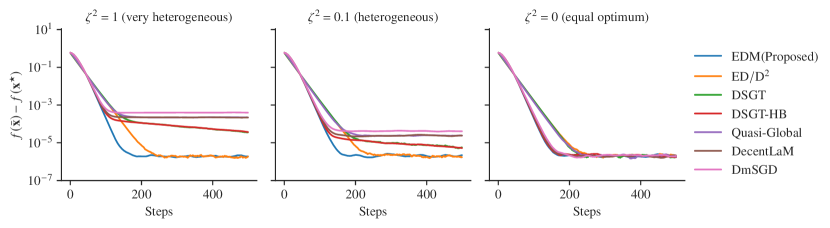
Figure 1: Quadratic loss function. We choose $\sigma^{2}=0.05$, $\alpha=0.05$, $\lambda=0.99$ and use different $\zeta^{2}$ to control the heterogeneity of $f_{i}$.

The experimental results indicate that all algorithms can converge linearly to a neighborhood of optimal values. However, as data heterogeneity increases, other momentum-based algorithms(DmSGD, Quasi-Global, and DecentLaM) become trapped in heterogeneous regions. Although the DSGT-HB algorithm effectively eliminates heterogeneity errors, its convergence rate is impacted by the original DSGT algorithm, resulting in momentum acceleration failure during the gradient consensus phase. In contrast, the EDM method retains the beneficial properties of the ED/D², and the introduction of momentum improves the algorithm’s convergence rate.

E.2 General Strongly Convex Loss

We consider the $\ell_{2}$-regularized logistic regression problem to investigate the algorithm’s convergence in a general strongly convex case. Let $\mathbf{x}_{i}\in\mathbb{R}^{d}$ be the local parameter of node $i$, and $\bm{\xi}_{i}=\{(\mathbf{u}_{ij}^{\top},v_{ij})^{\top}\}_{j=1,\cdots,m}$, where $u_{ij}\in\mathbb{R}^{d}$ is the covariate and $v_{ij}\in\{-1,1\}$ is the response. Given $\mathbf{x}_{i}$ and $\mathbf{u}_{ij}$, the response $v_{ij}$ is generated by $v_{ij}=1$ with probability $1/(1+\exp(-\mathbf{x}_{i}^{\top}\mathbf{u}_{ij}))$ and $v_{ij}=-1$ otherwise. The loss function at agent $i$ can be expressed as

$$f_{i}(\mathbf{x}_{i})=\frac{1}{m}\sum_{j=1}^{m}\log[1+\exp(-v_{ij}\mathbf{x}_{i}^{\top}\mathbf{u}_{ij})]+\frac{\mu}{2}\left\|\mathbf{x}_{i}\right\|^{2}.$$

It can be verified that the loss function is $\mu$-strongly convex.

Consider the following data generation methods to illustrate the heterogeneity of the data. Let $\mathbf{x}_{0}=(1,1,\cdots,1)^{\top}$, and generate $\bm{\epsilon}_{i}$ i.i.d. from $\mathcal{N}_{d}(0,\sigma_{h}^{2}I_{d})$, where $\sigma_{h}^{2}$ controls the heterogeneity of local parameter $\mathbf{x}_{i}$. We define $\mathbf{x}_{i}=\mathbf{x}_{0}+\bm{\epsilon}_{i}$. Additionally, the values $\{\mathbf{u}_{ij}\}$ are generated i.i.d. from $\mathcal{N}_{d}(0,I_{d})$. We then generate $z_{ij}$ i.i.d. from uniform distribution $\mathcal{U}(0,1)$. The variable $v_{ij}$ is set to 1 when$z_{ij}\leq 1/(1+\exp(-\mathbf{x}_{i}^{\top}\mathbf{u}_{ij}))$, and $-1$ otherwise.

In our approach, we utilize the full batch gradient $\nabla F(\mathbf{x}_{i},\bm{\xi}_{i})$ at every iteration. However, since we are using full batch samples, this results in no randomness. Thus, we add an additional i.i.d. noise term $\mathbf{s}_{i}^{(t)}$ drawn from $\mathcal{N}(0,\sigma_{s}^{2}I_{d})$ to $\nabla F(\mathbf{x}_{i}^{(t)},\bm{\xi}_{i})$. And use $\nabla F(\mathbf{x}_{i}^{(t)},\bm{\xi}_{i})+\mathbf{s}_{i}^{(t)}$ as the stochastic gradient. This method is similar to the one used in Alghunaim and Yuan (2022) to control the influence of gradient noise.

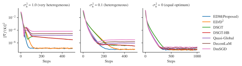
Figure 2: Logistic regression with $l_{2}$-regularization, random noise version. We choose $\sigma_{s}^{2}=0.01$, $\alpha=0.5$, $\lambda=0.99$, and use $\sigma_{h}^{2}$ to control the variance of $\mathbf{x}_{i}^{\star}$, which reflects the heterogeneity.

For our simulations, we set $d=20$ and $m=2000$, using the $\ell_{2}$-norm of the gradient $\|\nabla\bar{\mathbf{f}}(\overline{\mathbf{X}}^{(t)})\|_{2}^{2}$ as a measure of convergence. The simulation is conducted 20 times on a ring graph with $n=32$ nodes. We compare our method against DSGT, and ED/D², DSGT-HB and DmSGD. Figure 2 represents the result.

The simulation results demonstrate that our method can improve the performance of ED/D², and achieve convergence to a narrower region of global optimal values, with minimal influence from data heterogeneity.

E.3 Non-Convex Loss

Finally, we consider the non-convex condition. We deploy our method in a classification problem with deep neural networks and compare it with the aforementioned algorithms.

We use VGG-11 as the backbone network to train the classification task of the CIFAR10 dataset consisting of $N=50,000$ images of 10 labels, such as cats, airplanes, etc. The photos are $32\times 32$ size with three color channels. The criterion is the cross entropy. To quantitatively analyze the heterogeneity of the data in this dataset, we introduce the Dirichlet distribution, which is widely used to model heterogeneous scenarios for classification problems (Yurochkin et al., 2019; Lin et al., 2021). We generate $\mathbf{p}_{k}=(p_{k1},\cdots,p_{kn})$ for $k=1,\cdots,10$ from $\mathrm{Dirichlet}(\phi,\cdots,\phi)$, allocating $p_{ki}$ proportion of samples with label $k$ to agent $i$. The Dirichlet parameter $\phi$ is used to control the weights assigned to different categories of data across devices, serving as a measure of data heterogeneity. Specifically, a smaller value of $\phi$ indicates greater heterogeneity among the samples allocated to different agents. Our simulation for this part is primarily based on the code provided in Vogels et al. (2021).

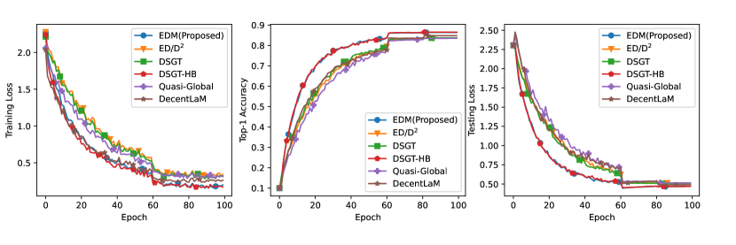
Figure 3: Classification of CIFAR10 by VGG11. Learning rate $\alpha=0.1$, heterogeneity parameter $\phi=1.0$ (heterogeneous).

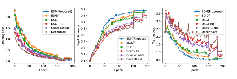
Figure 4: Classification of CIFAR10 by VGG11. Learning rate $\alpha=0.1$, heterogeneity parameter $\phi=0.1$ (very heterogeneous).

We considered two cases with $\phi=1$ (heterogeneous) and $\phi=0.1$ (highly heterogeneous). For $\phi=1$, the learning rate is reduced to 10% of its original value during the 60th and 80th epochs. In the case of $\phi=0.1$, the learning rate is similarly reduced to 10% of its original value at the 150th and 180th epochs. Each method is repeated three times, and the results are presented in Figures 3 and 4. Here the training loss is calculated as $\sum_{i=1}^{n}f_{i}(\mathbf{x}_{i}^{(t)})$. It is important to note that this selection reflects not the convergence properties of the algorithm, but rather whether the algorithm has fallen into the local minimum point for each agent $\mathbf{x}^{\star}_{i}$. In contrast, the testing loss provides a better indication of the convergence performance.

From the simulation results above, we can see that our algorithm outperforms other methods in the classification of CIFAR-10. Specifically, our proposed algorithm exceeds the performance of those that do not utilize momentum acceleration. When $\phi=1$, both our algorithm and DSGT-HB exhibit comparable convergence performance. However, as heterogeneity increases further ($\phi=0.1$), the convergence performance of DSGT-HB deteriorates significantly, even becoming inferior to that of the original algorithm. In contrast, our algorithm continues to demonstrate robust convergence properties. These findings are consistent with our theoretical analysis.

References

- Alghunaim and Yuan (2022) Alghunaim, S. A. and K. Yuan (2022). A unified and refined convergence analysis for non-convex decentralized learning. IEEE Transactions on Signal Processing 70, 3264–3279.
- Alghunaim and Yuan (2024) Alghunaim, S. A. and K. Yuan (2024). An enhanced gradient-tracking bound for distributed online stochastic convex optimization. Signal Processing 217, 109345.
- Ali et al. (2018) Ali, M. S., M. Vecchio, M. Pincheira, K. Dolui, F. Antonelli, and M. H. Rehmani (2018). Applications of blockchains in the internet of things: A comprehensive survey. IEEE Communications Surveys & Tutorials 21(2), 1676–1717.
- Beltrán et al. (2023) Beltrán, E. T. M., M. Q. Pérez, P. M. S. Sánchez, S. L. Bernal, G. Bovet, M. G. Pérez, G. M. Pérez, and A. H. Celdrán (2023). Decentralized federated learning: Fundamentals, state of the art, frameworks, trends, and challenges. IEEE Communications Surveys & Tutorials.
- Boyd et al. (2011) Boyd, S., N. Parikh, E. Chu, B. Peleato, J. Eckstein, et al. (2011). Distributed optimization and statistical learning via the alternating direction method of multipliers. Foundations and Trends® in Machine learning 3(1), 1–122.
- Gao and Huang (2020) Gao, H. and H. Huang (2020). Periodic stochastic gradient descent with momentum for decentralized training. arXiv preprint arXiv:2008.10435.
- Gao et al. (2023) Gao, J., X.-W. Liu, Y.-H. Dai, Y. Huang, and J. Gu (2023). Distributed stochastic gradient tracking methods with momentum acceleration for non-convex optimization. Computational Optimization and Applications 84(2), 531–572.
- Hsieh et al. (2020) Hsieh, K., A. Phanishayee, O. Mutlu, and P. Gibbons (2020). The non-iid data quagmire of decentralized machine learning. In International Conference on Machine Learning, pp. 4387–4398. PMLR.
- Huang et al. (2024) Huang, K., S. Pu, and A. Nedić (2024). An accelerated distributed stochastic gradient method with momentum. arXiv preprint arXiv:2402.09714.
- Jiang et al. (2017) Jiang, Z., A. Balu, C. Hegde, and S. Sarkar (2017). Collaborative deep learning in fixed topology networks. Advances in Neural Information Processing Systems 30.
- Koloskova et al. (2020) Koloskova, A., N. Loizou, S. Boreiri, M. Jaggi, and S. Stich (2020). A unified theory of decentralized sgd with changing topology and local updates. In International Conference on Machine Learning, pp. 5381–5393. PMLR.
- Lian et al. (2017) Lian, X., C. Zhang, H. Zhang, C.-J. Hsieh, W. Zhang, and J. Liu (2017). Can decentralized algorithms outperform centralized algorithms? a case study for decentralized parallel stochastic gradient descent. Advances in Neural Information Processing Systems 30.
- Lin et al. (2021) Lin, T., S. P. Karimireddy, S. Stich, and M. Jaggi (2021). Quasi-global momentum: Accelerating decentralized deep learning on heterogeneous data. In International Conference on Machine Learning, pp. 6654–6665. PMLR.
- Liu et al. (2020) Liu, Y., Y. Gao, and W. Yin (2020). An improved analysis of stochastic gradient descent with momentum. Advances in Neural Information Processing Systems 33, 18261–18271.
- Nedić et al. (2018) Nedić, A., A. Olshevsky, and M. G. Rabbat (2018). Network topology and communication-computation tradeoffs in decentralized optimization. Proceedings of the IEEE 106(5), 953–976.
- Nedic and Ozdaglar (2009) Nedic, A. and A. Ozdaglar (2009). Distributed subgradient methods for multi-agent optimization. IEEE Transactions on Automatic Control 54(1), 48–61.
- Nesterov (2013) Nesterov, Y. (2013). Introductory lectures on convex optimization: A basic course, Volume 87. Springer Science & Business Media.
- Polyak (1964) Polyak, B. T. (1964). Some methods of speeding up the convergence of iteration methods. Ussr Computational Mathematics and Mathematical Physics 4(5), 1–17.
- Polyak (1987) Polyak, B. T. (1987). Introduction to optimization. New York, Optimization Software.
- Pu and Nedić (2021) Pu, S. and A. Nedić (2021). Distributed stochastic gradient tracking methods. Mathematical Programming 187(1), 409–457.
- Sayed et al. (2014) Sayed, A. H. et al. (2014). Adaptation, learning, and optimization over networks. Foundations and Trends in Machine Learning 7(4-5), 311–801.
- Spiridonoff et al. (2020) Spiridonoff, A., A. Olshevsky, and I. C. Paschalidis (2020). Robust asynchronous stochastic gradient-push: Asymptotically optimal and network-independent performance for strongly convex functions. Journal of Machine Learning Research 21(58), 1–47.
- Takezawa et al. (2023) Takezawa, Y., H. Bao, K. Niwa, R. Sato, and M. Yamada (2023). Momentum tracking: Momentum acceleration for decentralized deep learning on heterogeneous data. Transactions on Machine Learning Research.
- Tang et al. (2018) Tang, H., X. Lian, M. Yan, C. Zhang, and J. Liu (2018). : Decentralized training over decentralized data. In International Conference on Machine Learning, pp. 4848–4856. PMLR.
- Vogels et al. (2021) Vogels, T., L. He, A. Koloskova, S. P. Karimireddy, T. Lin, S. U. Stich, and M. Jaggi (2021). Relaysum for decentralized deep learning on heterogeneous data. Advances in Neural Information Processing Systems 34, 28004–28015.
- Xin et al. (2020) Xin, R., S. Pu, A. Nedić, and U. A. Khan (2020). A general framework for decentralized optimization with first-order methods. Proceedings of the IEEE 108(11), 1869–1889.
- Yu et al. (2019) Yu, H., R. Jin, and S. Yang (2019). On the linear speedup analysis of communication efficient momentum sgd for distributed non-convex optimization. In International Conference on Machine Learning, pp. 7184–7193. PMLR.
- Yuan et al. (2020) Yuan, K., S. A. Alghunaim, B. Ying, and A. H. Sayed (2020). On the influence of bias-correction on distributed stochastic optimization. IEEE Transactions on Signal Processing 68, 4352–4367.
- Yuan et al. (2021) Yuan, K., Y. Chen, X. Huang, Y. Zhang, P. Pan, Y. Xu, and W. Yin (2021). Decentlam: Decentralized momentum sgd for large-batch deep training. In Proceedings of the IEEE/CVF International Conference on Computer Vision, pp. 3029–3039.
- Yuan et al. (2016) Yuan, K., Q. Ling, and W. Yin (2016). On the convergence of decentralized gradient descent. SIAM Journal on Optimization 26(3), 1835–1854.
- Yurochkin et al. (2019) Yurochkin, M., M. Agarwal, S. Ghosh, K. Greenewald, N. Hoang, and Y. Khazaeni (2019). Bayesian nonparametric federated learning of neural networks. In International Conference on Machine Learning, pp. 7252–7261. PMLR.
- Zhang and You (2019) Zhang, J. and K. You (2019). Decentralized stochastic gradient tracking for non-convex empirical risk minimization. arXiv preprint arXiv:1909.02712.