Temperature-Annealed Boltzmann Generators
Abstract
Efficient sampling of unnormalized probability densities such as the Boltzmann distribution of molecular systems is a longstanding challenge. Next to conventional approaches like molecular dynamics or Markov chain Monte Carlo, variational approaches, such as training normalizing flows with the reverse Kullback-Leibler divergence, have been introduced. However, such methods are prone to mode collapse and often do not learn to sample the full configurational space. Here, we present temperature-annealed Boltzmann generators (TA-BG) to address this challenge. First, we demonstrate that training a normalizing flow with the reverse Kullback-Leibler divergence at high temperatures is possible without mode collapse. Furthermore, we introduce a reweighting-based training objective to anneal the distribution to lower target temperatures. We apply this methodology to three molecular systems of increasing complexity and, compared to the baseline, achieve better results in almost all metrics while requiring up to three times fewer target energy evaluations. For the largest system, our approach is the only method that accurately resolves the metastable states of the system.
1 Introduction
Machine learning, and particularly generative models, have become a transformative force across numerous domains. A prime example of this impact is in structural biology, where deep learning methods such as those in the AlphaFold family Abramson et al., (2024), Jumper et al., (2021) have revolutionized our ability to predict protein structures. While a big part of AlphaFold’s success can surely be attributed to an advanced methodology, a key factor also lies in the availability of abundant experimental data, such as that in the Protein Data Bank (PDB) Burley et al., (2021).
However, not all scientific domains benefit from such well-curated and extensive experimental datasets. In areas where data scarcity is a persistent challenge, computational simulations play an essential role. Molecular dynamics (MD) and Markov chain Monte Carlo (MCMC) methods are the primary tools used to explore complex biochemical and physical systems and generate insights from limited experimental information. Despite their utility, these classical sampling approaches often come with significant computational costs, as they rely on iterative trajectory-based exploration of high-dimensional state spaces.
As a result, various approaches have been explored to speed up these methods, including integrating machine learning (ML)-based force fields Reiser et al., (2022), enhanced sampling techniques Barducci et al., (2011), and data-driven collective variables Bonati et al., (2021). Furthermore, (transferable) generative models have been trained on equilibrium samples from MD simulations Noé et al., (2019), Mahmoud et al., (2022), Klein and Noé, (2024), Zheng et al., (2023).
While these advancements have significantly improved the efficiency and utility of traditional simulations, there is a growing interest in rethinking the paradigm altogether. Variational sampling methods, rooted in generative modeling, offer a compelling alternative to classical MD and MCMC. These approaches aim to learn the underlying probability distribution without the availability of training data, bypassing the need for explicit trajectory-based sampling.
The most straightforward variational approach is to train a likelihood-based generative model, such as a normalizing flow, using the reverse Kullback-Leibler divergence (KLD). However, this is known to yield mode collapse in many scenarios Midgley et al., 2023b , Felardos et al., (2023). Recently, multiple variational sampling methods were developed Blessing et al., (2024), based on normalizing flows Midgley et al., 2023b , Matthews et al., (2023), diffusion models Akhound-Sadegh et al., (2024), Richter and Berner, (2024), Berner et al., (2024), Zhang et al., (2024), and flow matching Woo and Ahn, (2024).
Despite their promise to accelerate sampling, the applicability and scalability of variational sampling methods remain limited, and the field is in its early stages of development compared to the wealth of research on hybrid MD/ML approaches. To the best of our knowledge, the only variational approach that has successfully been applied to the sampling of molecular systems with non-trivial multimodality, such as the popular benchmark system alanine dipeptide, is Flow Annealed Importance Sampling Bootstrap (FAB) Midgley et al., 2023b .
In this work, we propose a novel and scalable flow-based framework to efficiently sample complex molecular systems without mode collapse. We train a normalizing flow at increased temperature using the reverse KLD, which we show reliably circumvents mode collapse. Since one is typically interested in the equilibrium distribution at lower temperatures, e.g. at room temperature, we introduce a reweighting-based training objective to iteratively anneal the distribution of the normalizing flow down to the target temperature. We demonstrate the capability and scalability of this methodology using three peptide systems of increasing complexity and achieve superior sampling efficiency and accuracy compared to baseline approaches.
Our contribution is threefold:
-
•
We show that, in contrast to current literature, the reverse KLD is surprisingly powerful at learning the Boltzmann distribution of molecular systems without mode-collapse, but only at increased temperatures where barriers between different free-energy minima are lower and the probability distribution maxima are interconnected.
-
•
We introduce an iterative reweighting-based training strategy to anneal the flow distribution to arbitrary target temperatures.
-
•
We introduce two complex molecular systems as new benchmarks that go far beyond the size of the typically used benchmark system alanine dipeptide, and we demonstrate that our approach scales to those systems without mode-collapse.
2 Related work
Leveraging the improved mode mixing behavior when sampling at higher temperatures is not a completely novel approach as it was introduced as an accelerated sampling technique for MCMC and MD simulations before. Replica exchange Markov chain Monte Carlo (RE-MCMC) and molecular dynamics (REMD) use multiple parallel trajectories (replicas) at different temperatures, while allowing repeated exchanges of configurations between the replicas. This essentially makes the high-temperature simulations help the lower-temperature simulations in overcoming slow energy barriers in the system.
Invernizzi et al., (2022) present a variation of replica exchange molecular dynamics using a normalizing flow that maps from the highest temperature replica directly to the target temperature. This allows direct exchanges and circumvents the need for intermediate replicas in the simulation. However, this still requires performing MD simulations at the boundary temperatures and it is not clear how well the method scales to larger systems.
Dibak et al., (2022) use a normalizing flow that is trained on samples from high-temperature molecular dynamics simulations. Using a special flow architecture, they show that the flow can be adapted to output low-temperature samples, even though it was only trained at the high temperature. Draxler et al., (2024) recently showed that the volume-preserving coupling layers used in that work are not universal, making the approach unsuitable for complex systems.
To solve this issue, Schebek et al., (2024) propose to use a normalizing flow with explicit conditioning on the temperature and pressure . The prior of the normalizing flow is formed by samples from an MD simulation at a reference thermodynamic state . The normalizing flow is subsequently trained to be able to sample across a range of thermodynamic states using the reverse KLD.
Similarly, Wahl et al., (2024) train a temperature-conditioned flow at increased temperature using samples from MD, and the correct temperature scaling to lower temperatures is obtained by matching the gradient of the unnormalized probability density of the flow with respect to the temperature to the gradient of the known target energy function.
So far, all mentioned approaches use (a large amount of) MD samples at at least one temperature, and transfer this to a different (lower) temperature. While a multitude of variational sampling methods that do not rely on samples from MD have been proposed Matthews et al., (2022), Midgley et al., 2023b , Akhound-Sadegh et al., (2024), to the best of our knowledge the only approach that has so far been successfully applied to non-trivial molecular systems is Flow Annealed Importance Sampling Bootstrap (FAB) by Midgley et al., 2023b ().
Instead of the reverse KLD, FAB uses the -divergence with for energy-based training. The -divergence is estimated using annealed importance sampling (AIS) from to , where Hamiltonian Monte Carlo (HMC) is used to transition between intermediate distributions. While AIS sampling is costly in terms of energy evaluations, it proved effective in learning complex probability distributions. They successfully learned the Boltzmann distribution of alanine dipeptide, a common benchmark molecular system, without mode collapse. However, how well this method scales to more complex systems is unclear, and we will address this in this work when comparing our approach to FAB.
3 Preliminaries
3.1 Normalizing Flows
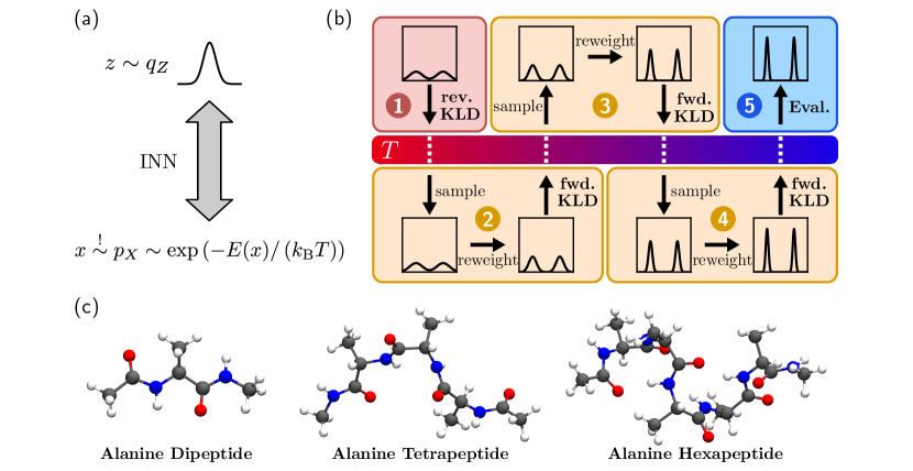
Normalizing flows use a latent distribution , typically a Gaussian or uniform distribution, which is transformed to the target space using an invertible transformation , (Figure 1a).
The transformed density of the flow can be expressed using the change of variables formula Dinh et al., (2015):
| (1) | |||
The most common approach to parametrize the invertible function is to use invertible coupling layers. In each coupling layer, the input is split into two parts and . The first part is transformed elementwise conditioned on the second part, while the second part is kept identical (see Figure 4 in the appendix for an illustration). If the elementwise transformation is invertible (monotonic), the whole transformation becomes invertible. Furthermore, the Jacobian matrix of such a coupling transform is lower triangular and can be efficiently computed.
Training by Example.
The key property of normalizing flows is that the likelihood (Equation 1) is directly available, typically at the cost of a forward pass. This allows data-based maximum likelihood training (forward KLD):
| (2) | |||
| (3) |
Training by Energy.
In this paper, we focus on the case where samples from the target distribution are not available, such that only the target density is known. In case of physical systems, such as the molecules studied in this work, this is the Boltzmann distribution . Here, is the 3D configuration of the molecule, for example the cartesian coordinates of all atoms, is the Boltzmann constant, is the temperature, and is the energy of the given configuration, evaluated either using quantum mechanics, e.g. with density functional theory, or, as in this work, using a parameterized force field. The reverse KLD can now be used to fit the distribution of the flow to the target density, using samples from the flow itself:
| (4) | |||
| (5) | |||
| (6) |
Since normalizing flows provide the likelihood of the generated samples, one can perform importance sampling to the true distribution using the importance weights . When estimating an expectation value of an observable using samples from the flow distribution , this offers asymptotically unbiased estimates Noé et al., (2019), Martino et al., (2017):
| (7) |
While diffusion models and continuous normalizing flows trained with flow-matching can provide likelihoods and can therefore also do importance sampling in theory, calculating the likelihoods is prohibitively expensive in practice, already for relatively small systems Klein and Noé, (2024).
While Equation 7 theoretically allows unbiased estimates, this is limited in practice by the actual overlap between the flow distribution and the target distribution . A helpful measure, here, is the effective sample size (ESS), defined as the number of independent samples needed from the target distribution to achieve the same variance in estimating expectation values as when using the flow distribution Martino et al., (2017). The reverse ESS is an approximation of the ESS, where samples from the flow are used (see Section E in the appendix). The ESS is thus only estimated within the support of the flow, meaning that a high ESS can still be achieved if only parts of the true distribution are covered. Therefore, the reverse ESS value needs to always be interpreted together with other metrics.
4 Methods
4.1 Flow architecture
Analogous to previous works Midgley et al., 2023b , Schopmans and Friederich, (2024), we use an internal coordinate representation based on bond lengths, angles, and dihedral angles to represent the molecular conformations. This incorporates the symmetries of the potential energy, which is invariant to translations and rotations of the whole molecule. For all experiments, we use a normalizing flow built from 16 monotonic rational-quadratic spline coupling layers Durkan et al., (2019) with fully connected parameter networks in the couplings. Dihedral angles are treated using circular splines Rezende et al., (2020) to incorporate the correct topology. Details can be found in Sections A and B of the appendix.
4.2 Temperature-Annealed Boltzmann Generators
Our approach to learn the Boltzmann distribution of molecular systems can be separated into two phases (see Figure 1b): First, we learn the distribution at a high temperature using the reverse KLD (see step 1 in Figure 1b). Due to decreased barrier heights, this can be done without mode collapse. Secondly, the distribution is iteratively annealed to obtain the distribution at the target temperature. We now explain both steps in detail and discuss why they avoid the challenges described above.
Training by Energy: Avoiding Mode Collapse
The mode-seeking behavior of the reverse KLD has been discussed and observed in multiple previous publications Midgley et al., 2023b , Felardos et al., (2023), Soletskyi et al., (2024). Once the flow collapsed to a mode, meaning that some remaining modes of the target distribution are not within the support of the flow, it will generally not escape this collapsed state if the remaining modes are too far separated from the collapsed mode. This is not surprising, since the reverse KLD is evaluated using an expectation value with samples from the flow distribution itself, which will only cover the collapsed modes.
At the typical target temperature for molecular systems, i.e. , modes are too far separated to be successfully covered with the reverse KLD. However, when sampling at increased temperature, the modes become more connected. Eventually, one can use the reverse KLD to efficiently learn the distribution. In this work, we therefore performed all reverse KLD experiments at . While it is possible to train models without mode collapse also at lower temperatures, we found to be suitable to obtain satisfying training stability without loss in accuracy.
Using any loss function that directly includes the target energy of a molecular system can be challenging. If two atoms overlap sufficiently, the repulsive van der Waals energy diverges, leading to unstable training. Following previous work Midgley et al., 2023b , we thus use a regularized energy function for training (see Section C in the appendix).
This avoids very high values in the loss function and stabilizes training. Furthermore, analogous to previous work Schopmans and Friederich, (2024), we found that removing a small fraction of the largest energy values in the loss contributions of each batch stabilizes training.
Reweighting-Based Annealing
As explained, we use the reverse KLD as a first step to learn the Boltzmann distribution at increased temperature. To obtain the distribution at a lower target temperature, here , we utilize importance sampling (Equation 7). While one could do importance sampling directly from to , this will yield bad overlap and sampling efficiency.
Instead, we perform importance sampling using multiple temperatures , where . In one annealing iteration, we perform the following steps:
-
1.
Sample a dataset of samples from the flow at the current temperature .
-
2.
Calculate importance weights for each sample in to transition to .
-
3.
According to these importance weights, resample a dataset with replacement from .
-
4.
Perform forward KLD training using .
With this buffered reweighting approach, we can anneal the distribution of the flow step by step toward the target temperature (see steps 2-4 in Figure 1b). To ensure a similar overlap between two consecutive distributions, we choose the temperatures using a geometric progression between and Sugita and Okamoto, (1999). For all experiments, we chose 9 temperature annealing steps.
Furthermore, we added a final fine-tuning step, where we sample at and reweight to . Empirically, this improves the final metrics obtained at . For the hexapeptide system, we added such fine-tuning steps after each annealing iteration. While this increases the total number of target potential energy evaluations, it improved the obtained results substantially. For the two less complex systems, intermediate fine-tuning was not necessary.
Variations
We note that our buffered reweighting approach is not the only option to anneal the temperature of a normalizing flow. As discussed in Section 2, a concurrent study Wahl et al., (2024) uses a temperature-conditioned normalizing flow with a temperature-scaling loss to learn the Boltzmann distribution at the target temperature. While this approach achieves promising results, it requires the repeated estimate of the partition function using importance sampling with the flow distribution. Obtaining a low-variance estimate of can be computationally expensive, especially for high-dimensional systems such as the hexapeptide studied here. However, a systematic comparison of different temperature scaling approaches is an interesting avenue for future work.
We further experimented with variations of our reweighting approach. For example, we tried training a temperature-conditioned flow with a reweighting-based objective continuously on the whole temperature range. This is described in more detail in Section 9 of the appendix. In practice, we found the iterative buffered annealing workflow to be superior, both in terms of accuracy and sampling efficiency.
5 Experiments
We now describe the conducted experiments to evaluate our temperature-annealing approach. The objective is to learn the Boltzmann distribution of three molecular systems, increasing in complexity (see Figure 1c). The first molecule is alanine dipeptide, a system that served as a benchmark in previous publications Midgley et al., 2023b , Wahl et al., (2024), Dibak et al., (2022). We further evaluate on two higher-dimensional and more complex systems, alanine tetrapeptide and alanine hexapeptide. All three systems have complex metastable high-energy regions that make up only a small fraction of the entire state space, which makes them suitable hard objectives for benchmarking.
5.1 Baseline methods
To judge the performance of our approach, we compare it to baseline methods. First, we trained a normalizing flow with the forward KLD using MD data from the target distribution. While this is not a variational sampling approach, it serves as a good baseline to show the expressiveness of the flow if data is available. Next, we trained a normalizing flow with the reverse KLD, targeting the Boltzmann distribution at . As the final and most powerful baseline, we trained Flow Annealed Importance Sampling Bootstrap (FAB) Midgley et al., 2023b . As already discussed, to the best of our knowledge, this is the only method that so far has shown success without mode collapse on our smallest test system alanine dipeptide. It therefore serves as a strong baseline.
5.2 Metrics
To evaluate the distribution of the normalizing flow at the target temperature , we use a combination of multiple metrics. First, we use the negative log-likelihood (NLL) calculated on the ground truth dataset. This is a good overall measure of the learned distribution. Furthermore, to assess potential mode collapse, we evaluate the free energy of the backbone dihedral angles (Ramachandran plots). Since these are the main slow degrees of freedom of the peptide systems, mode collapse will be directly visible here. To assess the quality of the Ramachandran plot, we calculate the forward KLD between the probability distribution given by the Ramachandran plot of the ground truth and the one of the flow distribution (RAM KLD). Since the tetrapeptide and hexapeptide have multiple pairs of backbone dihedral angles, we report the mean of their RAM KLD values. Furthermore, we repeat the calculation of the RAM KLD also using the Ramachandran plots obtained from importance sampling. Last, to evaluate the sampling efficiency, we report the reverse effective sample size (ESS) (see Section 3).
6 Results
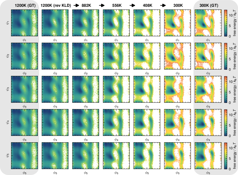
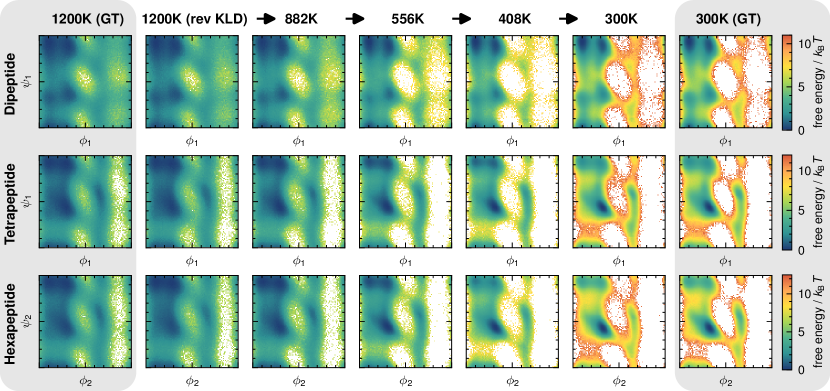
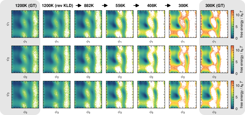
Figure 2 shows how the Ramachandran plots of each of the three systems are annealed to the target temperature, showing four exemplary steps of the annealing workflow. Both the distribution at learned with the reverse KLD and the distribution at the target temperature match the ground truth obtained from MD.
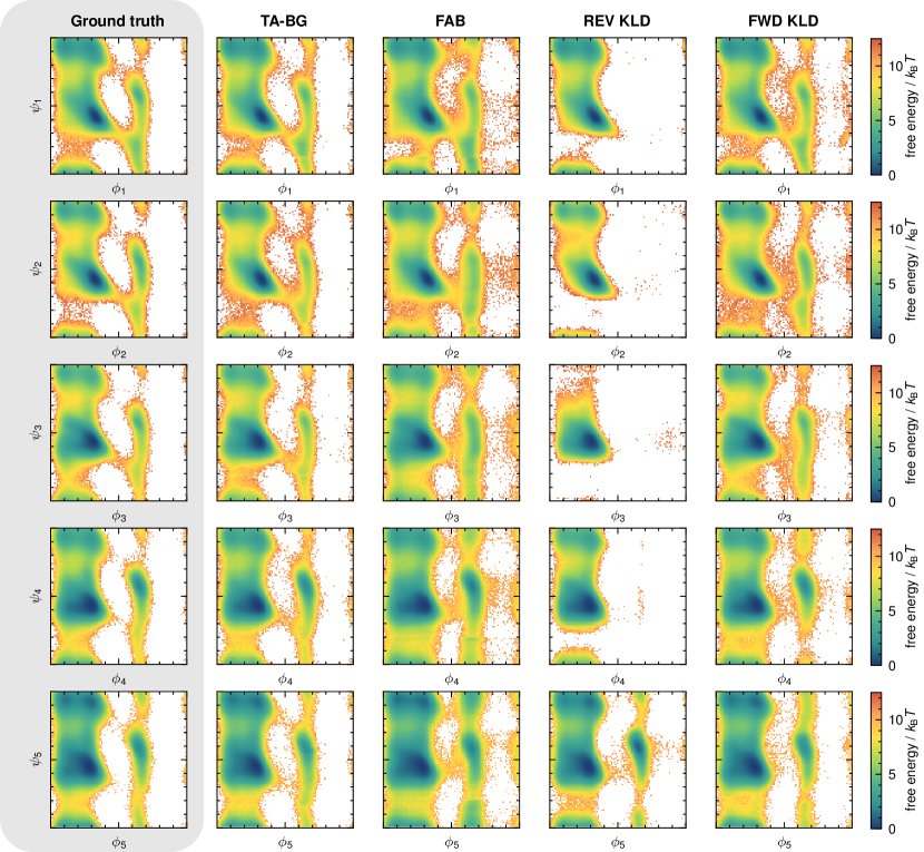
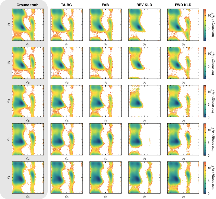
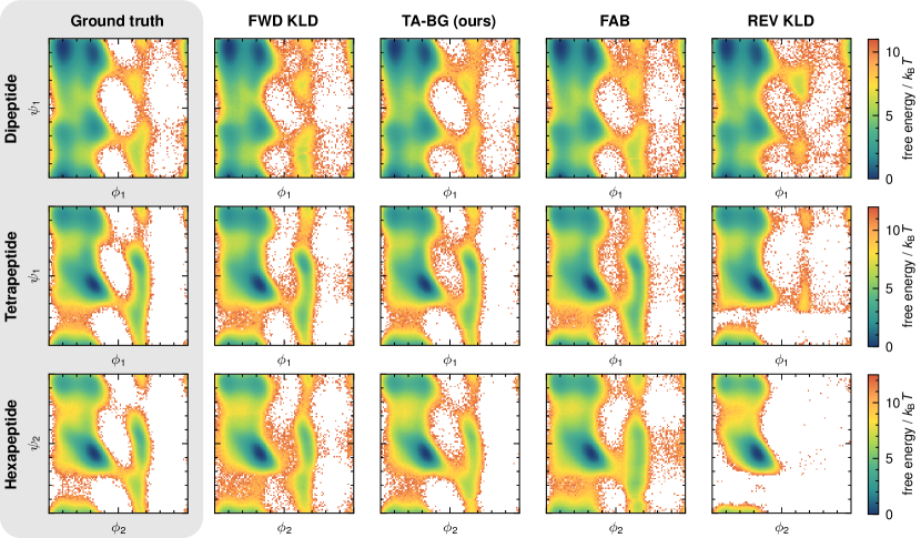
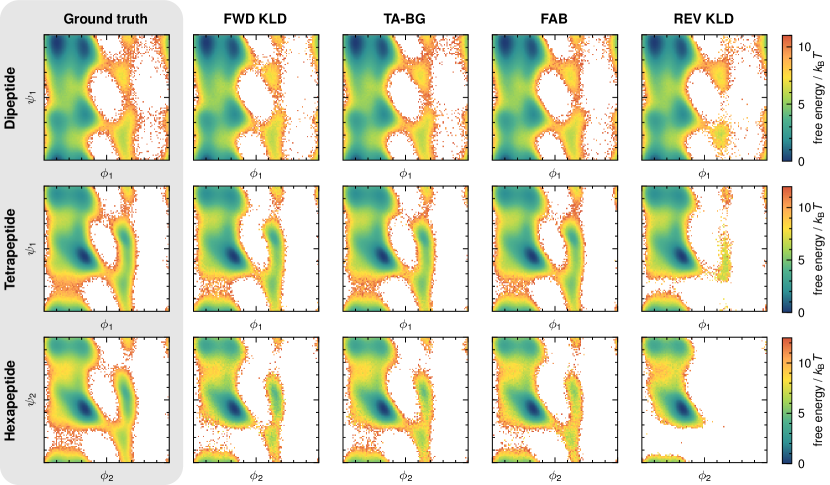
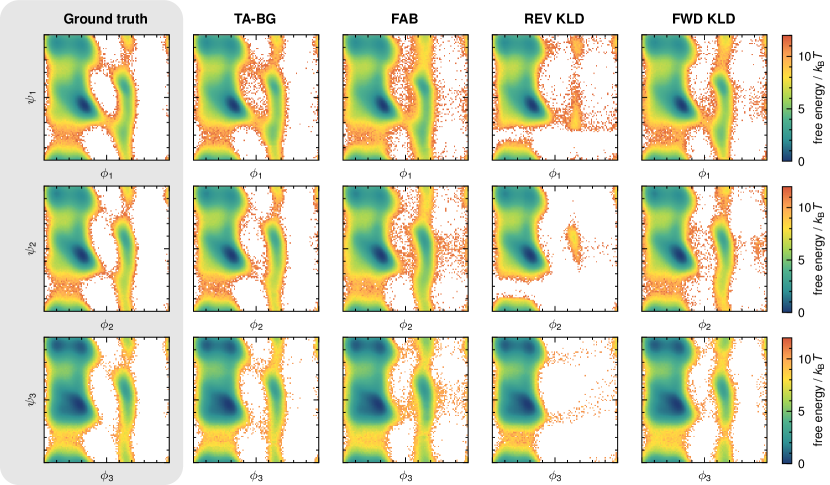
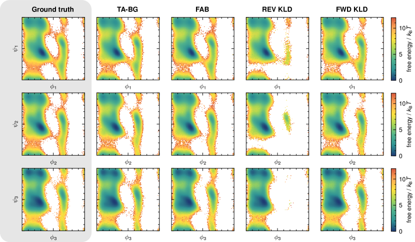
We now compare the obtained distribution at with that from the baseline methods by evaluating the introduced metrics (Table 1). Furthermore, Figure 3 shows the Ramachandran plots at obtained by all methods side by side. Figure 5 in the appendix shows the same comparison, but with importance sampling to the target distribution.
We start with the smallest system, alanine dipeptide. All methods, except for the reverse KLD, are able to learn the distribution without mode collapse (Figure 3). While the reverse KLD covers the high-energy region to some extent, partial mode collapse is visible. In terms of metrics, FAB and TA-BG obtain comparable results. Our method achieves better NLL and ESS values, while FAB achieves slightly lower RAM KLD values. Our approach only uses approximately a third of the target energy evaluations of FAB. We further note that the metrics we obtained with FAB on alanine dipeptide are slightly better but mostly comparable to those in the original publication.
Similar results can be observed for the tetrapeptide system. The reverse KLD training now collapses almost fully to the main mode, missing most of the metastable region (Figure 3). Both TA-BG and FAB achieve a good match with the ground truth distribution, fully resolving the metastable region. The metrics of TA-BG and FAB are again close, our approach achieves slightly better NLL and RAM KLD values, while FAB has a lower reweighted RAM KLD value and slightly higher ESS. Our approach again uses approximately a third of the target energy evaluations of FAB.
In case of the most complex investigated system, alanine hexapeptide, the distribution of the reverse KLD training again almost entirely collapses. While FAB is partially able to resolve the metastable states, they differ in shape compared to the ground truth distribution. In contrast, our approach covers all metastable states without mode collapse and resolves them accurately with only small imperfections. This is also reflected and quantified by the metrics: Compared to FAB, our approach achieves better results in all metrics, while requiring target energy evaluations compared to used by FAB.
A tradeoff exists between the accuracy of the obtained distribution and the number of target evaluations. This is especially true for FAB, where the number of intermediate AIS distributions and the number of HMC steps can be varied. We present corresponding variations in Table 9 in the appendix. For FAB applied to the hexapeptide, even when using almost 3 times as many target evaluations compared to our approach, we still achieve a lower NLL value.
| System | Method | PE EVALS | NLL | ESS / % | Ram KLD | Ram KLD w. RW |
|---|---|---|---|---|---|---|
| dipeptide | forward KLD | |||||
| reverse KLD | ||||||
| FAB | ||||||
| TA-BG (ours) | ||||||
| Tetra- peptide | forward KLD | |||||
| reverse KLD | ||||||
| FAB | ||||||
| TA-BG (ours) | ||||||
| Hexa- peptide | forward KLD | |||||
| reverse KLD | ||||||
| FAB | ||||||
| TA-BG (ours) |
7 Discussion
We start our discussion by pointing out the surprisingly good results we obtained by simply training with the reverse KLD at for alanine dipeptide (Figure 3). Even though at the metastable states are only connected to the global minimum by a very low-probability transition region, only partial mode collapse is observed. Next to our results of being able to successfully learn the distribution at high temperatures with the reverse KLD, this further shows the effectiveness of simple reverse KLD training.
Furthermore, previous work showed that not only training a normalizing flow from scratch with the reverse KLD is prone to mode collapse, but also fine-tuning a pre-trained flow with the reverse KLD to a target distribution typically collapses Felardos et al., (2023). This is a not-well-understood phenomenon and has only recently been investigated theoretically Soletskyi et al., (2024). While Felardos et al., (2023) proposed a solution to this problem by introducing a novel loss function, it is not clear how well this scales to larger systems. As described before, after our annealing workflow reaches , we fine-tune the flow distribution at by performing forward KLD training with a buffered dataset from the flow distribution, reweighted to the target distribution. This offers a simple yet effective solution to the problem of fine-tuning pre-trained flows and can also be used in other scenarios. For example, one can train a flow on biased MD simulation data that is not properly equilibrated, and then fine-tune with our buffered reweighting approach to obtain an unbiased flow distribution.
Furthermore, while our method generally yielded better results with fewer target energy evaluations for the hexapeptide, the results we obtained using FAB are still relatively close in terms of accuracy, especially for the other two systems. This establishes it as a powerful method for variational sampling. Therefore, a combination of our temperature-annealing approach with FAB is an interesting avenue for future work. Instead of using the reverse KLD for training at increased temperatures, FAB can be used and the distribution can be subsequently annealed with our TA-BG workflow. If and when this can be better than simple reverse KLD training at high temperatures needs to be investigated.
A current limitation of our work is the use of an internal coordinate representation, which is not transferable between systems. A transferable equivariant normalizing flow has recently been proposed Midgley et al., 2023a . This might turn out to be a superior choice for scaling to even larger systems. Additionally, our results indicate that also other variational sampling approaches, such as those based on diffusion models, could benefit from sampling at higher temperatures. While here our reweighting-based temperature-annealing workflow can not be directly applied, since computing exact likelihoods for these models is prohibitively expensive, alternative temperature-scaling losses similar to that introduced by Wahl et al., (2024) could be used.
8 Conclusion
We introduced temperature-annealed Boltzmann generators, a technique that uses a combination of high-temperature reverse KLD training with an annealing workflow to efficiently sample the Boltzmann distribution of molecular systems at room temperature. On the molecular systems investigated, our approach achieves better results in almost all metrics, while requiring up to three times fewer target energy evaluations compared to the baselines. Furthermore, it was the only variational approach that accurately resolved the metastable region of the most complex system studied, demonstrating its scaling capabilities from toy examples to application-relevant systems.
Similar to how replica-exchange molecular dynamics is an established method in the toolbox of computational scientists, we are confident that high-temperature sampling with temperature-annealing is a powerful approach that will move the field of variational sampling forward.
Software and Data
All source code to reproduce the shown experiments will be made available on GitHub soon. Furthermore, we will publish all ground-truth MD trajectories.
References
- Bgf, (2024) (2024). Bgflow. AI4Science group, FU Berlin (Frank Noé and co-workers).
- Abramson et al., (2024) Abramson, J., Adler, J., Dunger, J., Evans, R., Green, T., Pritzel, A., Ronneberger, O., Willmore, L., Ballard, A. J., Bambrick, J., Bodenstein, S. W., Evans, D. A., Hung, C.-C., O’Neill, M., Reiman, D., Tunyasuvunakool, K., Wu, Z., Žemgulytė, A., Arvaniti, E., Beattie, C., Bertolli, O., Bridgland, A., Cherepanov, A., Congreve, M., Cowen-Rivers, A. I., Cowie, A., Figurnov, M., Fuchs, F. B., Gladman, H., Jain, R., Khan, Y. A., Low, C. M. R., Perlin, K., Potapenko, A., Savy, P., Singh, S., Stecula, A., Thillaisundaram, A., Tong, C., Yakneen, S., Zhong, E. D., Zielinski, M., Žídek, A., Bapst, V., Kohli, P., Jaderberg, M., Hassabis, D., and Jumper, J. M. (2024). Accurate structure prediction of biomolecular interactions with AlphaFold 3. Nature, 630(8016):493–500.
- Akhound-Sadegh et al., (2024) Akhound-Sadegh, T., Rector-Brooks, J., Bose, J., Mittal, S., Lemos, P., Liu, C.-H., Sendera, M., Ravanbakhsh, S., Gidel, G., Bengio, Y., Malkin, N., and Tong, A. (2024). Iterated Denoising Energy Matching for Sampling from Boltzmann Densities. In Forty-First International Conference on Machine Learning.
- Barducci et al., (2011) Barducci, A., Bonomi, M., and Parrinello, M. (2011). Metadynamics. WIREs Computational Molecular Science, 1(5):826–843.
- Berner et al., (2024) Berner, J., Richter, L., and Ullrich, K. (2024). An optimal control perspective on diffusion-based generative modeling.
- Blessing et al., (2024) Blessing, D., Jia, X., Esslinger, J., Vargas, F., and Neumann, G. (2024). Beyond ELBOs: A Large-Scale Evaluation of Variational Methods for Sampling. In Forty-First International Conference on Machine Learning.
- Bonati et al., (2021) Bonati, L., Piccini, G., and Parrinello, M. (2021). Deep learning the slow modes for rare events sampling. Proceedings of the National Academy of Sciences, 118(44):e2113533118.
- Burley et al., (2021) Burley, S. K., Bhikadiya, C., Bi, C., Bittrich, S., Chen, L., Crichlow, G. V., Christie, C. H., Dalenberg, K., Di Costanzo, L., Duarte, J. M., Dutta, S., Feng, Z., Ganesan, S., Goodsell, D. S., Ghosh, S., Green, R. K., Guranović, V., Guzenko, D., Hudson, B. P., Lawson, C. L., Liang, Y., Lowe, R., Namkoong, H., Peisach, E., Persikova, I., Randle, C., Rose, A., Rose, Y., Sali, A., Segura, J., Sekharan, M., Shao, C., Tao, Y.-P., Voigt, M., Westbrook, J. D., Young, J. Y., Zardecki, C., and Zhuravleva, M. (2021). RCSB Protein Data Bank: Powerful new tools for exploring 3D structures of biological macromolecules for basic and applied research and education in fundamental biology, biomedicine, biotechnology, bioengineering and energy sciences. Nucleic Acids Research, 49(D1):D437–D451.
- Conor Durkan et al., (2020) Conor Durkan, Artur Bekasov, Iain Murray, and George Papamakarios (2020). Nflows: Normalizing flows in PyTorch.
- D.A. Case et al., (2023) D.A. Case, H.M. Aktulga, K. Belfon, I.Y. Ben-Shalom, J.T. Berryman, S.R. Brozell, D.S. Cerutti, T.E. Cheatham, III, V.W.D. Cruzeiro, T.A. Darden, N. Forouzesh, G. Giambasu, T. Giese, M.K. Gilson, H. Gohlke, A.W. Goetz, J. Harris, S. Izadi, S.A. Izmailov, K. Kasavajhala, M.C. Kaymak, E. King, A. Kovalenko, T. Kurtzman, T.S. Lee, P. Li, C. Lin, J. Liu, T. Luchko, R. Luo, M. Machado, V. Man, M. Manathunga, K.M. Merz, Y. Miao, O. Mikhailovskii, G. Monard, H. Nguyen, K.A. O’Hearn, A. Onufriev, F. Pan, S. Pantano, R. Qi, A. Rahnamoun, D.R. Roe, A. Roitberg, C. Sagui, S. Schott-Verdugo, A. Shajan, J. Shen, C.L. Simmerling, N.R. Skrynnikov, J. Smith, J. Swails, R.C. Walker, J. Wang, J. Wang, H. Wei, X. Wu, Y. Wu, Y. Xiong, Y. Xue, D.M. York, S. Zhao, Q. Zhu, and P.A. Kollman (2023). Amber 2023. University of California, San Francisco.
- Dibak et al., (2022) Dibak, M., Klein, L., Krämer, A., and Noé, F. (2022). Temperature steerable flows and Boltzmann generators. Phys. Rev. Res., 4(4):L042005.
- Dinh et al., (2015) Dinh, L., Krueger, D., and Bengio, Y. (2015). NICE: Non-linear Independent Components Estimation.
- Draxler et al., (2024) Draxler, F., Wahl, S., Schnoerr, C., and Koethe, U. (2024). On the Universality of Volume-Preserving and Coupling-Based Normalizing Flows. In Forty-First International Conference on Machine Learning.
- Durkan et al., (2019) Durkan, C., Bekasov, A., Murray, I., and Papamakarios, G. (2019). Neural Spline Flows.
- Eastman et al., (2024) Eastman, P., Galvelis, R., Peláez, R. P., Abreu, C. R. A., Farr, S. E., Gallicchio, E., Gorenko, A., Henry, M. M., Hu, F., Huang, J., Krämer, A., Michel, J., Mitchell, J. A., Pande, V. S., Rodrigues, J. P., Rodriguez-Guerra, J., Simmonett, A. C., Singh, S., Swails, J., Turner, P., Wang, Y., Zhang, I., Chodera, J. D., De Fabritiis, G., and Markland, T. E. (2024). OpenMM 8: Molecular Dynamics Simulation with Machine Learning Potentials. J. Phys. Chem. B, 128(1):109–116.
- Felardos et al., (2023) Felardos, L., Hénin, J., and Charpiat, G. (2023). Designing losses for data-free training of normalizing flows on Boltzmann distributions.
- Invernizzi et al., (2022) Invernizzi, M., Krämer, A., Clementi, C., and Noé, F. (2022). Skipping the Replica Exchange Ladder with Normalizing Flows. J. Phys. Chem. Lett., 13(50):11643–11649.
- Jumper et al., (2021) Jumper, J., Evans, R., Pritzel, A., Green, T., Figurnov, M., Ronneberger, O., Tunyasuvunakool, K., Bates, R., Žídek, A., Potapenko, A., Bridgland, A., Meyer, C., Kohl, S. A. A., Ballard, A. J., Cowie, A., Romera-Paredes, B., Nikolov, S., Jain, R., Adler, J., Back, T., Petersen, S., Reiman, D., Clancy, E., Zielinski, M., Steinegger, M., Pacholska, M., Berghammer, T., Bodenstein, S., Silver, D., Vinyals, O., Senior, A. W., Kavukcuoglu, K., Kohli, P., and Hassabis, D. (2021). Highly accurate protein structure prediction with AlphaFold. Nature, 596(7873):583–589.
- Kingma and Ba, (2017) Kingma, D. P. and Ba, J. (2017). Adam: A Method for Stochastic Optimization.
- Klein and Noé, (2024) Klein, L. and Noé, F. (2024). Transferable Boltzmann Generators.
- Mahmoud et al., (2022) Mahmoud, A. H., Masters, M., Lee, S. J., and Lill, M. A. (2022). Accurate Sampling of Macromolecular Conformations Using Adaptive Deep Learning and Coarse-Grained Representation. J. Chem. Inf. Model., 62(7):1602–1617.
- Martino et al., (2017) Martino, L., Elvira, V., and Louzada, F. (2017). Effective Sample Size for Importance Sampling based on discrepancy measures. Signal Processing, 131:386–401.
- Matthews et al., (2022) Matthews, A., Arbel, M., Rezende, D. J., and Doucet, A. (2022). Continual Repeated Annealed Flow Transport Monte Carlo. In Proceedings of the 39th International Conference on Machine Learning, pages 15196–15219. PMLR.
- Matthews et al., (2023) Matthews, A. G. D. G., Arbel, M., Rezende, D. J., and Doucet, A. (2023). Continual Repeated Annealed Flow Transport Monte Carlo.
- (25) Midgley, L. I., Stimper, V., Antorán, J., Mathieu, E., Schölkopf, B., and Hernández-Lobato, J. M. (2023a). SE(3) Equivariant Augmented Coupling Flows. In Thirty-Seventh Conference on Neural Information Processing Systems.
- (26) Midgley, L. I., Stimper, V., Simm, G. N. C., Schölkopf, B., and Hernández-Lobato, J. M. (2023b). Flow Annealed Importance Sampling Bootstrap. In The Eleventh International Conference on Learning Representations.
- Noé et al., (2019) Noé, F., Olsson, S., Köhler, J., and Wu, H. (2019). Boltzmann generators: Sampling equilibrium states of many-body systems with deep learning. Science, 365(6457):eaaw1147.
- Paszke et al., (2019) Paszke, A., Gross, S., Massa, F., Lerer, A., Bradbury, J., Chanan, G., Killeen, T., Lin, Z., Gimelshein, N., Antiga, L., Desmaison, A., Köpf, A., Yang, E., DeVito, Z., Raison, M., Tejani, A., Chilamkurthy, S., Steiner, B., Fang, L., Bai, J., and Chintala, S. (2019). PyTorch: An Imperative Style, High-Performance Deep Learning Library.
- Reiser et al., (2022) Reiser, P., Neubert, M., Eberhard, A., Torresi, L., Zhou, C., Shao, C., Metni, H., van Hoesel, C., Schopmans, H., Sommer, T., and Friederich, P. (2022). Graph neural networks for materials science and chemistry. Commun Mater, 3(1):1–18.
- Rezende et al., (2020) Rezende, D. J., Papamakarios, G., Racaniere, S., Albergo, M., Kanwar, G., Shanahan, P., and Cranmer, K. (2020). Normalizing Flows on Tori and Spheres. In Proceedings of the 37th International Conference on Machine Learning, pages 8083–8092. PMLR.
- Richter and Berner, (2024) Richter, L. and Berner, J. (2024). Improved sampling via learned diffusions.
- Schebek et al., (2024) Schebek, M., Invernizzi, M., Noé, F., and Rogal, J. (2024). Efficient mapping of phase diagrams with conditional Boltzmann Generators. Mach. Learn.: Sci. Technol., 5(4):045045.
- Schopmans and Friederich, (2024) Schopmans, H. and Friederich, P. (2024). Conditional Normalizing Flows for Active Learning of Coarse-Grained Molecular Representations. In Forty-First International Conference on Machine Learning.
- Soletskyi et al., (2024) Soletskyi, R., Gabrié, M., and Loureiro, B. (2024). A theoretical perspective on mode collapse in variational inference.
- Stimper et al., (2022) Stimper, V., Midgley, L. I., Simm, G. N. C., Schölkopf, B., and Hernández-Lobato, J. M. (2022). Alanine dipeptide in an implicit solvent at 300K.
- Sugita and Okamoto, (1999) Sugita, Y. and Okamoto, Y. (1999). Replica-exchange molecular dynamics method for protein folding. Chemical Physics Letters, 314(1):141–151.
- Wahl et al., (2024) Wahl, S., Rousselot, A., Draxler, F., and Köthe, U. (2024). TRADE: Transfer of Distributions between External Conditions with Normalizing Flows.
- Woo and Ahn, (2024) Woo, D. and Ahn, S. (2024). Iterated Energy-based Flow Matching for Sampling from Boltzmann Densities.
- Zhang et al., (2024) Zhang, D., Chen, R. T. Q., Liu, C.-H., Courville, A., and Bengio, Y. (2024). Diffusion Generative Flow Samplers: Improving learning signals through partial trajectory optimization.
- Zheng et al., (2023) Zheng, S., He, J., Liu, C., Shi, Y., Lu, Z., Feng, W., Ju, F., Wang, J., Zhu, J., Min, Y., Zhang, H., Tang, S., Hao, H., Jin, P., Chen, C., Noé, F., Liu, H., and Liu, T.-Y. (2023). Towards Predicting Equilibrium Distributions for Molecular Systems with Deep Learning.
Appendix A Internal coordinate representation
As discussed in the main text, we use an internal coordinate representation based on bond lengths, angles, and dihedral angles to represent the conformations of the molecular systems. As discussed in the next section, we use splines as the invertible transformations in our coupling blocks. These splines are only defined for mappings from the interval to . Therefore, we scale all internal coordinates to fit in this range (here, ).
To achieve this, we divide all dihedral angles by . Furthermore, bond lengths and angles are transformed as
| (8) |
Here, is the value of the corresponding degree of freedom from a minimum energy structure obtained from minimizing the initial structure with the force field. was empirically chosen as for bond length dimensions and for angle dimensions.
For the peptides studied in this work, two chiral forms (mirror images) exist. In nature, one almost exclusively finds only one of the two (L-form). However, since the potential energy is invariant to the mirror symmetry, there is no preference given by the energy model itself. Previous work Midgley et al., 2023b , Schopmans and Friederich, (2024) simply filtered the “wrong” R-chirality during training. In contrast, we directly constrain generation to the L-chirality by restricting the output bounds of the splines that generate the dihedrals of the hydrogens at the chiral centers to the range . For this, we transform the corresponding dimensions as after the flow generated them. This entirely removes the R-chirality from the space the flow can generate.
Furthermore, there is no preference given for the permutation of hydrogens in \ceCH3 groups. However, since the ground truth molecular dynamics simulations start from a given starting configuration, a preference does exist in the ground truth. Therefore, we restrict the generated distribution of the flow to this preference, by constraining the spline output range of the respective dihedral angles, analogous to how we constrain the chirality (see above).
Appendix B Architecture
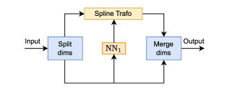
For the normalizing flow architecture, we use a similar architecture to previous works Midgley et al., 2023b , Schopmans and Friederich, (2024). As the invertible transformation in the coupling layers we use monotonic rational-quadratic splines Durkan et al., (2019) that map the interval to using monotonically increasing rational-quadratic functions in bins. The dihedral angles are treated with periodic boundaries in the range Rezende et al., (2020).
We use 8 pairs of neural spline coupling layers. In each pair, we use a randomly generated mask to decide which dimensions to transform and which dimensions to condition the transformation on (see Figure 4). In the second coupling of each pair, the inverted mask is used. The dimensions of the dihedral angles are treated using circular splines Rezende et al., (2020) to incorporate the correct topology. After each coupling layer, we add a random (but fixed) periodic shift to the dihedral angle dimensions.
The latent distribution of the normalizing flow is a uniform distribution in the range for the dihedral angle dimensions, and a Gaussian distribution with and , truncated to the range , for the bond length and angle dimensions.
As the conditioning network ( in Figure 4), we use a fully connected neural network with hidden dimensions [256,256,256,256,256] and ReLU activation functions. Previous works used a fully connected neural network with a skip connection Midgley et al., 2023b , Schopmans and Friederich, (2024), however, we found no benefit in this and therefore did not use a skip connection. To incorporate their periodicity, dihedral angles are represented as before being passed as input to the neural network.
We used the same architecture for all experiments of all methods. The number of parameters in the architecture of each system can be found in Table 2.
| Alanine Dipeptide | Alanine Tetrapeptide | Alanine Hexapeptide | |
|---|---|---|---|
| Number of parameters |
Appendix C Molecular Systems
| Name | Sequence | NO. atoms | NO. hydrogens | NO. bonds | NO. angles | NO. torsions |
|---|---|---|---|---|---|---|
| alanine dipeptide | ACE-ALA-NME | 22 | 12 | 21 | 20 | 19 |
| alanine tetrapeptide | ACE-3ALA-NME | 42 | 22 | 19 (+ 22) | 40 | 39 |
| alanine hexapeptide | ACE-5ALA-NME | 62 | 32 | 29 (+ 32) | 60 | 59 |
To avoid diverging van der Waals energies due to atom clashes, we train with a regularized energy function Midgley et al., 2023b :
| (9) |
For all systems, we used the energy regularization parameters (Equation 9) and .
Appendix D Force Field and Ground Truth Simulations
All ground truth simulations have been performed with OpenMM 8.0.0 Eastman et al., (2024) using the CUDA platform. Ground truth energy evaluations during training have been performed with 18 workers in parallel using the OpenMM CPU Platform.
Details on the simulation and force field parameters for each system can be found in Table 4. For all systems, we used different variants of Amber force fields D.A. Case et al., (2023). For alanine dipeptide, the parameters are identical to the ones used in the FAB publication Midgley et al., 2023b . Therefore, here we use the dataset made available by Stimper et al., (2022). Additionally to this ground truth dataset used for evaluation, we performed an additional simulation for alanine dipeptide at (see Table 4). We used for equilibration and a production simulation time of . The small time step of was chosen since this system does not use hydrogen bond length constraints. This additional dataset was used for training the forward KLD experiments.
The force field parameters of the alanine tetrapeptide system match those used in the temperature steerable flow publication Dibak et al., (2022). However, no public dataset for this system was available, which is why we performed two replica-exchange molecular dynamics (REMD) simulations to obtain reliable ground truth data. The hexapeptide system was, to the best of our knowledge, not used in previous publications, so we also here performed REMD simulations to obtain a ground truth dataset for evaluation. All REMD simulations used equilibration without exchanges, equilibration with exchanges, and for the production simulation. For both the tetrapeptide and hexapeptide, we used one simulation for ground truth evaluation, and the other simulation to perform the forward KLD experiments.
Additionally to the simulations performed to obtain the data for evaluation, we performed higher-temperature simulations to evaluate the temperature scaling and the reverse KLD training at (see Table 4).
All ground truth datasets at contain samples, subsampled randomly from the total MD trajectory. All training datasets used for the forward KLD experiments contain samples.
| System | Force-field | Constraints | / | Sim. time / | Time step / |
|---|---|---|---|---|---|
| alanine dipeptide | AMBER ff96 with OBC1 implicit solvation | None | 300 | ||
| 800 | |||||
| 1200 | |||||
| alanine tetrapeptide | AMBER99SB-ILDN with AMBER99 OBC implicit solvation | Hydrogen bond lengths | 300, 332, 368, 408, 451, 500 (REMD) | ||
| 800 | |||||
| 1200 | |||||
| alanine hexapeptide | AMBER99SB-ILDN with AMBER99 OBC implicit solvation | Hydrogen bond lengths | 300, 332, 368, 408, 451, 500 (REMD) | ||
| 800 | |||||
| 1200 |
Appendix E Metrics details
RAM KLD
To obtain comparable results to those in the original FAB publication Midgley et al., 2023b , we evaluated the forward KLD of the Ramachandran plots in the same way. First, we calculated the probability density of the Ramachandran plot of the ground truth and that of the flow distribution on a x grid, using samples for both. Then, the forward KLD is calculated between the two distributions.
RAM KLD W. RW
We repeat the same procedure to assess the obtained Ramachandran plot after reweighting to the target distribution. Here, analogous to Midgley et al., 2023b (), we clipped the highest importance weights to the lowest value among them. This is necessary because of outliers in the importance weights due to flow numerics.
ESS
The ESS was calculated according to the following equation Midgley et al., 2023a :
| (10) | |||
Also here, we clipped the highest importance weights to the lowest value among them.
While one can also calculate the forward ESS, which uses samples from the ground truth Midgley et al., 2023a , in practice we found this metric to yield spurious results, depending heavily on the chosen importance weight clipping value. Therefore, we chose to only use the reverse ESS, even though it does not capture mode collapse.
Appendix F TA-BG variations
As described in the main text, next to our buffered iterative annealing workflow, we also tried training a temperature- conditioned normalizing flow on the whole continuous temperature range. To fix the distribution at at the distribution learned by the reverse KLD, we use a split architecture to train with temperature-conditioning:
-
•
A base flow generates samples at . This was trained with the reverse KLD at , and the weights of this base are frozen for the next step.
-
•
A head flow is added to the “base“ flow, which transforms the high-temperature samples to lower temperatures. The spline couplings of the head flow are scaled in such a way that they always output the identity for .
In each batch, we sampled a support temperature and a target temperature and performed reweighted forward KLD training:
| (11) |
We also used this training objective with self-normalized weights within each batch, and with resampling each batch according to the importance weights.
The training objective in Equation 11 is similar to the one introduced by Wahl et al., (2024), but does not require the estimate of the partition function for evaluation. In practice, however, we found the iterative annealing workflow to yield more accurate results, while also being more sampling efficient compared to using Equation 11.
A systematic comparison of using Equation 11 and using the training objective introduced by Wahl et al., (2024) can be explored in future work.
Appendix G Hyperparameters
All experiments used the Adam optimizer Kingma and Ba, (2017).
| Dipeptide | Tetrapeptide | Hexapeptide | Dipeptide | Tetrapeptide | Hexapeptide | |
| gradient descent steps | ||||||
| learning rate | ||||||
| batch size | 1024 | 1024 | 1024 | 256 | 256 | 512 |
| grad norm clipping | 100.0 | 100.0 | 100.0 | 100.0 | 100.0 | 100.0 |
| lr linear warmup steps | 1000 | 1000 | 1000 | 1000 | 1000 | 1000 |
| weight decay (L2) | ||||||
| NO. highest energy values removed | 40 | 40 | 40 | 10 | 10 | 20 |
| Dipeptide | Tetrapeptide | Hexapeptide | |
|---|---|---|---|
| gradient descent steps | |||
| learning rate | |||
| batch size | 1024 | 1024 | 1024 |
G.1 TA-BG
| Dipeptide | Tetrapeptide | Hexapeptide | |
| gradient descent steps per annealing step | |||
| learning rate | |||
| batch size | 2048 | 4096 | 2048 |
| LR scheduler | cosine annealing | - | - |
| buffer samples drawn per annealing step | |||
| buffer resampled to |
In all TA-BG experiments, we used the following annealing steps:
As described in the main text, the hexapeptide additionally used also intermediate fine-tuning steps after each annealing step.
As described in the main text, in each step of the annealing workflow we use a buffered dataset for training, resampled according to the importance weights from samples drawn from the flow distribution. Similarly to how we clipped the importance weights to calculate the forward KLD of the reweighted Ramachandrans, also here we clipped the highest of the importance weights to the lowest value among them.
G.2 FAB
For the FAB experiments, we started from the hyperparameters reported in the original publication. To make the original FAB hyperparameters a good starting point, we scaled our internal coordinates from [0,1] to [-5,5], which was the range used in the FAB source code. With this, we used an initial HMC step size of 0.1 for all experiments. Since FAB obtained significantly better results by using a prioritized replay buffer, and we were able to reproduce this finding, we chose the same replay buffer used originally by FAB for all experiments. Furthermore, all experiments used a cosine annealing learning rate scheduler with a single cycle.
| Dipeptide | Tetrapeptide | Hexapeptide | |
| gradient descent steps | |||
| learning rate | |||
| batch size | 1024 | 1024 | 1024 |
| grad norm clipping | 1000.0 | 1000.0 | 1000.0 |
| lr linear warmup steps | 1000 | 1000 | 1000 |
| weight decay (L2) | |||
| NO. intermed. dist. | 8 | 8 | 8 |
| NO. inner hmc steps | 4 | 4 | 8 |
Appendix H FAB hyperparameter variations
As with most sampling approaches, the number of target evaluations and the accuracy of the obtained distribution is a tradeoff. Especially for the hexapeptide, FAB was not able to resolve the metastable high-energy states accurately. Therefore, we performed additional experiments where we varied the number of intermediate distributions and the number of HMC steps. This improves the results slightly, while requiring significantly more target energy evaluations (see Table 9).
For the smaller systems, alanine dipeptide and alanine tetrapeptide, we further performed experiments with smaller batch sizes while using the same number of gradient descent steps. This lowers the number of required target energy evaluations. However, as one can see from Table 9, this comes at the cost of further increasing the NLL.
| System | batch size | NO. intermed. | NO. inner | PE EVALS | NLL | |
|---|---|---|---|---|---|---|
| dist. | HMC steps | |||||
| alanine dipeptide | 1024 | 8 | 4 | |||
| 512 | 8 | 4 | ||||
| 256 | 8 | 4 | ||||
| alanine tetrapeptide | 1024 | 8 | 4 | |||
| 512 | 8 | 4 | ||||
| 256 | 8 | 4 | ||||
| alanine hexapeptide | 1024 | 8 | 4 | |||
| 512 | 8 | 4 | ||||
| 1024 | 16 | 4 | ||||
| 1024 | 8 | 8 | ||||
| 1024 | 16 | 8 |
Appendix I Additional Figures
I.1 Alanine Tetrapeptide
I.2 Alanine Hexapeptide