coupledMatrixFoam: a foam-extend-based fully-implicit solver for heterogeneous porous media

Abstract

The study of multiphase flows in porous media is fundamental to various fields, including oil recovery, CO₂ sequestration, hydrogeology, and others. Accurate predictions of fluid behavior in these systems can enhance process efficiency while mitigating environmental and health risks. In this context, numerical simulation serves as a powerful tool for anticipating complex flow phenomena and optimizing engineering strategies. Both commercial simulators and open-source softwares, such as the porousMultiphaseFoam repository based on the OpenFOAM framework, have been developed to model these processes. However, simulating heterogeneous porous media with complex porosity and permeability distributions poses significant numerical challenges. To address these, we introduce coupledMatrixFoam, a new OpenFOAM-based solver designed for enhanced robustness and numerical stability. coupledMatrixFoam integrates the Eulerian multi-fluid formulation for phase fractions with Darcy’s law for porous media flow, employing a fully implicit, block-coupled solution for the governing equations. Built on Foam-extend 5.0, it leverages the latest fvBlockMatrix developments to improve computational efficiency. This approach enables a significant increase in time step sizes, particularly in cases involving capillary pressure effects and other complex physical interactions. This work details the development, implementation, and validation of coupledMatrixFoam, including comparisons with porousMultiphaseFoam to assess performance improvements. Additionally, a scalability analysis is conducted, demonstrating the solver’s suitability for high-performance computing (HPC) applications, which are essential for large-scale, real-world simulations.

1 Introduction

Multiphase flows in porous media systems are related to a great variety of engineering applications such as oil production, underground aquifers, CO2 sequestration, fuel cells, porous concrete, bed filters, and others [1]. Several computational models for simulating such types of flows have been proposed [2], and open-source porous media simulators developed. Examples of open-source frameworks and libraries are DuMux [3], MRST [4], OpenGeoSys [5], PFlotran [6], Open Porous Media [7], and MOOSE (PorousFlow module) [8]. In the same way as the aforementioned initiatives, this paper presents an open repository that contains a set of computational codes for porous media flow simulations. The repository, called porousMedia, has been developed by WIKKI Brasil in the OpenFOAM framework [9, 10].

Various open-source codes have been developed in the OpenFOAM framework for porous media applications (see, for example, [11, 12, 13, 14, 15]). Considering those related to oil production, which is our main application of interest, we can mention the well-known porousMultiphaseFoam toolbox, introduced in [16] for the simulation of incompressible two-phase flows in porous media, and then extended to adaptive mesh refinement [17], black-oil model [18], hydrogeological flows modeling [19], two-phase systems containing porous and solid-free regions [20], and fracture models [21]. In this work, we present the coupledMatrixFoam, a new OpenFOAM solver for the simulation of fully coupled multiphase flow and transport in heterogeneous porous media, typical of oil production scenarios. The introduced solver is based on the Euler-Euler multi-fluid model for physical systems of $n$ phase fractions [22], as well as the solver we presented in the preliminary work [23]. Our solvers differ from other approaches by modeling the porous medium as a stationary phase that composes the system. Moreover, here we address a unique contribution in terms of computational efficiency by solving pressure and all phase fractions simultaneously throughout a fully implicit implementation that applies the block matrix framework of Foam-extend version 5.0 [24].

coupledMatrixFoam solver considers the Euler-Euler model for a system of phase fractions combined with Darcy’s law for flows through porous media [25], defining the rock system as a set of stationary phases. The code implementation is based on the very used multiphaseEulerFoam application [26], a choice that can benefit future extensions such as phase compressibility, multiple species, heat, and mass transfer. In line with our previous works [23] and [27], the proposed solver has important functionalities related to porous media modeling and simulation, including support for heterogeneous permeability and porosity fields and specialized models for relative permeability and capillary pressure. Furthermore, the solution approach introduced here couples the phase fractions and pressure solution in order to achieve substantial improvements in computational efficiency for scenarios characterized by high complexity in terms of porosity, permeability, and capillary pressure effects.

For simulating multiphase flows there are generally sequential and coupled approaches. Sequential approaches, such as the Implicit Pressure Explicit Saturation (IMPES, [28]), simplify the numerical solution procedures by splitting operators, but presents severe time step limitations. On the other hand, coupled schemes are more complex as they solve the same system of equations simultaneously, but guarantee stability enabling higher advances in time [29]. Newton methods combined with preconditioner strategies are popular for solving multiphase flow equations implicitly in the context of porous media [30, 31, 32]. In the current work, we use Taylor series expansions to linearize pressure and phase fractions dependencies, solving the resulting linearized system by a structure based on the latest development aimed at coupled solutions in foam-extend (fvBlockMatrix). Analogous linearization procedures have been used to solve velocity and stress tensor coupling for laminar viscoelastic flows in [33], and to treat implicit relation between phase fractions for multiphase flows in [34, 35]. Related works that use the block-coupled matrix structure of foam-extend include a transient implicit pressure-velocity coupling scheme for the Eulerian fluid model with any number of phases [36]; a selective Algebraic Multigrid solver applied to the implicitly coupled steady-state incompressible pressure-velocity system [37]; and a coupled pressure based solution algorithm to model interface capturing problems [38]. Note that the works developed in OpenFOAM cited above do not deal with applications in porous media, which reinforces the importance of the cases to be studied using the coupledMatrixFoam.

The fully implicit algorithm developed has the potential of improving code’s robustness significantly when compared to segregated strategies. This paper provides great details about the formulation and implementation of the solver, along with validation studies. Besides that, effectiveness of the implemented methodology is demonstrated by notable improvements in the average time step, resulting in substantial reductions in computational costs. Additionally, a scalability analysis is conducted, demonstrating the solver’s suitability for HPC applications. Therefore, this work contributes to the advancement of computational efficiency in solving multiphase flows in porous media, particularly in scenarios with complex geometries and significant capillary pressure effects.

The paper is divided into the following sections. The mathematical model is presented in Section 2, followed by the numerical formulation and implementation aspects in Section 3. Detailed information about the computational code are provided in Section 4, numerical results in Section 5, and conclusions in Section 6.

2 Mathematical model

2.1 General equations

In the context of porous media flows, the momentum balance equation of each phase fraction reduces to Darcy’s law

$$\alpha_{i}\mathbf{U}_{i}=-\frac{k_{r,i}}{\mu_{i}}\mathbf{K}\cdot(\nabla p_{i}-\rho_{i}\mathbf{g})$$ (1)

where $\mathbf{U}$ is the velocity, $\alpha$ is the phase fraction, $k_{r}$ the relative permeability, $\mathbf{K}$ the absolute permeability, $p$ the total pressure, $\rho$ the density, $\mu$ is the dynamic viscosity and $\mathbf{g}$ the gravity. The sub-index $i$ indicates the phase. Considering a system of incompressible phases, the mass balance equation for each phase is given as:

$$\frac{\partial\alpha_{i}}{\partial t}+\nabla\cdot\left(\alpha_{i}\mathbf{U}_{i}\right)=0.$$ (2)

Substituting Eqn.(1) in Eqn.(2), the new form of the phase continuity equation is given by:

$$\frac{\partial\alpha_{i}}{\partial t}-\nabla\cdot\left(\frac{k_{r,i}}{\mu_{i}}\mathbf{K}\cdot(\nabla p_{i}-\rho_{i}\mathbf{g})\right)=0.$$ (3)

Eqn.(3) is the final equation for the transport of each phase fraction. Note that the velocity fields were removed and it’s no more necessary to solve them.

It is important to highlight that in multiphase systems there exists the constraint

$$\sum_{p=1}^{N_{p}}\alpha_{p}=1,$$ (4)

where $N_{p}$ is the total number of phases in the multiphase system. Another relevant concept is the mixture velocity $\mathbf{U}_{m}$ which, for $n$ phases, is given by

$$\mathbf{U}_{m}=\sum_{i=1}^{n}\alpha_{i}\mathbf{U}_{i}.$$ (5)

The mass conservation of the incompressible system can be defined as zero divergent of the mixture velocity

$$\nabla\cdot\left(\mathbf{U}_{m}\right)=0.$$ (6)

Substituting Eqn.(1) in Eqn.(5) and then, the resultant equation in Eqn.(6), we obtain

$$-\nabla\cdot\left[\sum_{i=1}^{N_{P}}\left(\frac{k_{r,i}}{\mu_{i}}\mathbf{K}\cdot(\nabla p_{i}-\rho_{i}\mathbf{g})\right)\right]=0.$$ (7)

Usually in OpenFOAM codes, Eqn.(7) is used as the pressure equation of the system. In summary, the mathematical model for incompressible multiphase flows in porous media is composed by the transport equations of phase fractions, Eqn.(3), the relationship between phase fractions, Eqn.(4), and the pressure equation, Eqn.(7).

2.2 Stationary phases

Aiming to explore the advantages of the Euler-Euler methodology, the porous media is modeled as a stationary phase. Considering a null velocity for this type of phase, the continuity equation is given by:

$$\dfrac{\partial\alpha_{s}}{\partial t}=Q_{\alpha_{s}},$$ (8)

where the sub-index $s$ indicates a stationary phase and $Q_{\alpha_{s}}$ is a source term, which is zero in the cases considered in this paper but will be used in future extensions to include compressibility, mass transfer, and other effects. It is possible to observe that Eqn.(8) is a diagonal equation, with simple and cheap solution.

Generally, computational codes for porous media are based on porosity ($\phi$), but the coupledMatrixFoam is based on phase fractions. The relation is given by

$$\phi=\alpha_{v},$$ (9)

where $\alpha_{v}$ is the void volumetric fraction, calculated as

$$\alpha_{v}=1-\sum_{k=1}^{N_{s}}\alpha_{k},$$ (10)

considering $N_{s}$ the number of stationary phases in the system.

The consideration of stationary phases to model the porous media is strategically interesting as it is possible to use the foam-extend structure for the phase system both in these phases.

2.3 Effects of relative permeability

A comprehensive framework for multiphase flows, involving any number of phases, necessitates relative permeability models for each fluid-rock interface. The widely used Brooks and Corey (BC) model [39] relates the relative permeability of each phase to the phase fraction as follows:

$$k_{r,i}=k_{r,i(\text{max})}\left(\frac{\alpha_{i}}{\alpha_{v}}\right)^{\eta},$$ (11)

where $\eta$ is a power coefficient associated with the porous media properties, $\alpha_{v}$ is the void volumetric fraction, and $k_{r,i(\text{max})}$ is the maximal relative permeability.

By substituting Eqn. (11) into the pressure Eqn. (7), one obtains:

$$-\nabla\cdot\left[\sum_{i=1}^{N_{P}}\left(\frac{k_{r,i(\text{max})}}{\mu_{i}}\left(\frac{\alpha_{i}}{\alpha_{v}}\right)^{\eta}\mathbf{K}\cdot(\nabla p_{i}-\rho_{i}\mathbf{g})\right)\right]=0.$$ (12)

In similar way, substituting Eqn. (11) into the transport Eqn. (3):

$$\frac{\partial\alpha_{i}}{\partial t}-\nabla\cdot\left(\frac{k_{r,i(\text{max})}}{\mu_{i}}\left(\frac{\alpha_{i}}{\alpha_{v}}\right)^{\eta}\mathbf{K}\cdot(\nabla p_{i}-\rho_{i}\mathbf{g})\right)=0.$$ (13)

Equations (12) and (13) introduce a nonlinear term between pressure and phase fraction in the system of equations, requiring special treatment. Additionally, the coupledMatrixFoam framework supports the use of tabulated methodology, where users can provide a table with the relative permeability values as a function of saturation $S_{i}=\alpha_{i}/\alpha_{v}$.

2.4 Capillary effects

The discontinuity between two moving phases in a porous multiphase flow gives rise to an additional relationship between pressure fields known as capillary pressure $p_{c}$, given by:

$$p_{c,ki}=p_{k}-p_{i},$$ (14)

where $k$ is a reference phase for the capillary pressure and $i$ represents any other phase in the system. Thus, the pressure of the reference phase $k$ and the capillary pressure of the pair $ki$ are used to define the pressure of any phase $i$. Replacing the pressure of a phase, $p_{i}$, in Eqn.(12) and Eqn.(13), respectively, by the definition of capillary pressure in Eqn.(14), one can write:

$$-\nabla\cdot\left[\sum_{i=1}^{N_{P}}\left(\frac{k_{r,i(\text{max})}}{\mu_{i}}\left(\frac{\alpha_{i}}{\alpha_{v}}\right)^{\eta}\mathbf{K}\cdot(\nabla p_{k}-\nabla p_{c,ki}-\rho_{i}\mathbf{g})\right)\right]=0$$ (15)

and

$$\frac{\partial\alpha_{i}}{\partial t}-\nabla\cdot\left(\frac{k_{r,i(\text{max})}}{\mu_{i}}\left(\frac{\alpha_{i}}{\alpha_{v}}\right)^{\eta}\mathbf{K}\cdot(\nabla p_{k}-\nabla p_{c,ki}-\rho_{i}\mathbf{g})\right)=0.$$ (16)

It is worthy noting that for the reference phase, capillary pressure satisfies $p_{c,kk}=0$, and hence Equations (12) and (13) remain unchanged.

A useful approximation to the capillary pressure is to consider that it depends only on saturation, and hence

$$\nabla p_{c,ki}=\frac{\partial p_{c,ki}}{\partial S_{i}}\nabla S_{i}.$$ (17)

Since the mathematical formulation of the solver developed is based on phase fractions, not in saturation, so, one more manipulation is necessary for Eqn. (17). Considering that the saturation of a phase $i$ is given by $S_{i}=\alpha_{i}/\alpha_{v}$, we can writte

$$\nabla p_{c,ki}=\frac{\partial p_{c,ki}}{\partial S_{i}}\left(\frac{\nabla\alpha_{i}}{\alpha_{v}}-\frac{\alpha_{i}\nabla\alpha_{v}}{\alpha_{v}^{2}}\right).$$ (18)

In this way, it is possible to add the capillarity effect without adding new variables to the system of equations. However, the capillarity models must be able to provide the derivative of capillary pressure as a function of saturation.

3 Numerical formulation and implementation

Numerical formulation and implementation aspects applied to treat different terms to be inserted into the block system resulting from the implicit coupling of pressure and phase fractions will be described in this section.

3.1 Linearization for non-linear terms

In the coupled formulation, non-linear terms require a linearization to construct a linear system of equations to be operated by the solver. The Taylor Approximation (TA) method, as applied by Keser et al. [34], was employed to linearize these terms.

To use Taylor expansions of functions in the coupled problem considered here, we suppose that the variables $\alpha_{i}$ and $p$ can be expressed, respectively, as $\alpha_{i}^{n}=\alpha_{i}^{o}+\Delta\alpha_{i}$ and $p^{n}=p^{o}+\Delta p$, where the superscript $n$ indicates the new approximate value (in the current time-step/iteration), $o$ indicates the old value (from the previous time-step/iteration), and $\Delta$ is a small correction. The first-order Taylor series expansion of the pressure and phase fraction unknowns can be expressed as

$$f(\alpha_{i}^{n},p^{n})\approx f(\alpha_{i}^{o},p^{o})+\Delta\alpha_{i}\dfrac{\partial f(\alpha_{i}^{o},p^{o})}{\partial\alpha_{i}}+\Delta p\dfrac{\partial f(\alpha_{i}^{o},p^{o})}{\partial p}.$$ (19)

Considering that the goal is to obtain the value in the current time, the corrections could be expressed as $\Delta\alpha_{i}=\alpha_{i}^{n}-\alpha_{i}^{o}$ and $\Delta p=p^{n}-p^{o}$. Besides this consideration, the function $f$ can be written in the following form:

$$f(\alpha_{i}^{n},p^{n})=\alpha_{i}^{n}\,p^{n}\,\Upsilon(\alpha_{i}^{o},p^{o}),$$ (20)

where $\alpha_{i}^{n}\,p^{n}$ is the implicit part of $f$, and $\Upsilon(\alpha_{i}^{o},p^{o})$ represents the explicit part. Substituting the variations and Eqn. (20) in Eqn. (19), the Taylor expansion is given by:

$$f(\alpha_{i}^{n},p^{n})\approx\alpha_{i}^{o}\,p^{o}\,\Upsilon(\alpha_{i}^{o},p^{o})+(\alpha_{i}^{n}-\alpha_{i}^{o})\dfrac{\partial(\alpha_{i}^{o}\,p^{o}\,\Upsilon(\alpha_{i}^{o},p^{o}))}{\partial\alpha_{i}}+(p^{n}-p^{o})\dfrac{\partial(\alpha_{i}^{o}\,p^{o}\,\Upsilon(\alpha_{i}^{o},p^{o}))}{\partial p},$$ (21)

that leads to

$$f(\alpha_{i}^{n},p^{n})\approx\alpha_{i}^{n}p^{o}\,\Upsilon(\alpha_{i}^{o},p^{o})+\alpha_{i}^{o}\,p^{n}\,\Upsilon(\alpha_{i}^{o},p^{o})-\alpha_{i}^{o}\,p^{o}\,\Upsilon(\alpha_{i}^{o},p^{o}).$$ (22)

Therefore, TA divides the nonlinear terms involving pressure and phase fractions into three components: explicit, implicit, and cross-coupling.

3.2 Handling coupled unknowns

Since the solution algorithm proposed here employs a linear solver, the non-linear terms must be linearized. The application of the methodology described in subsection 3.1 for treating nonlinear terms will be detailed following.

The non-linear terms to be treated are present in the pressure Eqn.(15) and transport Eqn.(16). To facilitate the implementation process, it is introduced an auxiliary variable $\mathbf{T}_{i}$ for each phase $i$ of the system, which is defined as:

$$\mathbf{T}_{i}=\frac{k_{r,i(\text{max})}}{\mu_{i}\alpha_{i}}\left(\frac{\alpha_{i}}{\alpha_{v}}\right)^{\eta}\mathbf{K}.$$ (23)

Note that by using $\mathbf{T}_{i}$ in Eqn.(15) and Eqn.(16), we obtain, respectively:

$$-\nabla\cdot\left[\sum_{i=1}^{N_{P}}\left(\alpha_{i}\mathbf{T}_{i}\cdot(\nabla p_{k}-\nabla p_{c,ki}-\rho_{i}\mathbf{g})\right)\right]=0$$ (24)

and

$$\frac{\partial\alpha_{i}}{\partial t}-\nabla\cdot\left(\alpha_{i}\mathbf{T}_{i}\cdot(\nabla p_{k}-\nabla p_{c,ki}-\rho_{i}\mathbf{g})\right)=0.$$ (25)

Therefore, the non-linear terms to be treated have been rewritten in the form

$$\alpha_{i}\mathbf{T}_{i}\cdot(\nabla p_{k}-\nabla p_{c,ki}-\rho_{i}\mathbf{g}).$$ (26)

Next, we explain the different aspects to be considered for each nonlinear term of Eqn.(26).

3.2.1 Pressure term

The non-linear term involving phase fraction $\alpha_{i}$ and reference phase pressure, here denoted by $p$ for simplicity, can be handled using TA. To linearize such term, we assume that $\mathbf{T}_{i}$ can be calculated explicitly using the phase fraction approximation from the previous time-step/iteration (denoted by the superscript $o$). Thus, the non-linear term between phase fraction and pressure at the current time-step/iteration (denoted by the superscript $n$) is given by:

$$\left(\alpha_{i}\,\mathbf{T}_{i}\cdot\nabla p\right)^{n}\approx\mathbf{T}_{i}^{o}\cdot(\alpha_{i}^{n}\nabla p^{o}+\alpha_{i}^{o}\nabla p^{n}-\alpha_{i}^{o}\nabla p^{o}).$$ (27)

It is important to emphasize that the relative permeability model generally is highly dependent on phase fraction values, and hence, the implicit treatment for $\alpha_{i}$ in the product $\alpha_{i}\mathbf{T}_{i}$ is crucial to ensure improvements to the accuracy and stability of the system.

3.2.2 Gravity term

In phase fraction and pressure equations, there is also consideration of gravitational effects on the flow, modeled by the term $\alpha_{i}\,\rho_{i}\,\mathbf{T}_{i}\cdot\mathbf{g}$ in Eqn.(26). The simplest way to handle this term would be to add its effect explicitly. However, using an explicit approach to treat key terms in the system can lead to significant reductions in the time step, reducing the computational efficiency. An alternative way that we use to linearize it, which depends implicitly on the phase fraction, is given by:

$$\left(\alpha_{i}\,\rho_{i}\,\mathbf{T}_{i}\cdot\mathbf{g}\right)^{n}\approx\alpha_{i}^{n}\,\rho_{i}^{o}\,\mathbf{T}_{i}^{o}\cdot\mathbf{g}.$$ (28)

Thus, the phase fraction is evaluated at the current time ($\alpha_{i}^{n}$), which avoids a fully explicit treatment of the gravity-related term, resulting in less impact on the stability and robustness of the implemented code.

3.2.3 Capillary pressure term

The non-linear term involving phase fraction and capillary pressure in Eqn.(26) is $\alpha_{i}\mathbf{T}_{i}\cdot\nabla p_{c,ki}$. Substituting Eqn.(18) into the referred term and rearranging it, the capillary pressure contribution can be written as:

$$\alpha_{i}\,\frac{\partial p_{c,i}}{\partial S_{i}}\,\mathbf{T}_{i}\cdot\left(\frac{\nabla\alpha_{i}}{\alpha_{v}}-\frac{\alpha_{i}\nabla\alpha_{v}}{\alpha_{v}^{2}}\right),$$ (29)

where the sub-index $k$ related to the reference phase has been omitted for the sake of simplicity.

Equation (29) can be separated into two terms, and both need to be treated through linearizations. For the first term, one possibility is to treat the phase fraction multiplying the partial derivative of capillary pressure with respect to saturation as information obtained from the previous iteration ($\alpha_{i}^{o}$):

$$\left(\alpha_{i}\,\frac{\partial p_{c,i}}{\partial S_{i}}\,\mathbf{T}_{i}\cdot\frac{\nabla\alpha_{i}}{\alpha_{v}}\right)^{n}\approx\alpha_{i}^{o}\,\left(\frac{\partial p_{c,i}}{\partial S_{i}}\right)^{o}\,\mathbf{T}_{i}^{o}\cdot\frac{\nabla\alpha_{i}^{n}}{\alpha_{v}^{o}}.$$ (30)

The second alternative is to apply the TA, taking the phase fraction and the gradient of phase $i$ implicitly. Following this approach, the first term can be linearized as:

$$\left(\alpha_{i}\,\frac{\partial p_{c,i}}{\partial S_{i}}\,\mathbf{T}_{i}\cdot\frac{\nabla\alpha_{i}}{\alpha_{v}}\right)^{n}\approx\frac{1}{\alpha_{v}^{o}}\,\left(\frac{\partial p_{c,i}}{\partial S_{i}}\right)^{o}\,\mathbf{T}_{i}^{o}\cdot\left(\alpha_{i}^{o}\nabla\alpha_{i}^{n}+\alpha_{i}^{n}\nabla\alpha_{i}^{o}\ -\alpha_{i}^{o}\nabla\alpha_{i}^{o}\right),$$ (31)

where the presence of three parcels: coupling, implicit, and explicit is observed when applying the methodology.

During the development of the code, both alternatives were compared in different scenarios and no difference was observed in terms of stability, robustness, or accuracy. So, considering that the first linearization is cheaper, it was the option implemented in the final version of the code. It is important to highlight that the second treatment could be beneficial for some future implementations in the code, so, the possibility to use the second treatment is open.

Finally, in the linearization of the second term in Eqn.(29), only one of the phase fractions $\alpha_{i}$ will be considered at the current time, resulting in:

$$\left(-\alpha_{i}\alpha_{i}\,\frac{\partial p_{c,i}}{\partial S_{i}}\,\mathbf{T}_{i}\cdot\frac{\nabla\alpha_{v}}{\alpha^{2}_{v}}\right)^{n}\approx-\alpha_{i}^{n}\alpha_{i}^{o}\,\left(\frac{\partial p_{c,i}}{\partial S_{i}}\right)^{o}\,\mathbf{T}_{i}^{o}\cdot\left(\frac{\nabla\alpha_{v}}{\alpha_{v}^{2}}\right)^{o}.$$ (32)

We remark that the void fraction $\alpha_{v}$ does not change throughout the entire simulation since effects such as compressibility and mass transfer in the porous medium are not considered in the current version of the code. For this reason, the evaluation of the void fraction can always use the value from the previous iteration or time step. The same reasoning has been applied to all other terms where this parameter appears.

3.3 The final system of equations

With all terms properly linearized, it is possible to write the final system of equations, which will later be assembled into a block matrix. The final format for each equation of the system is presented below.

3.3.1 Reference moving phase

In order to ensure the constrain Eqn.(4), a moving phase $\alpha_{R}$ is chosen as a reference phase and obtained by the relationship:

$$\alpha_{R}=1-\sum_{p=1}^{N_{p}-1}\alpha_{p},$$ (33)

instead of being solved by the transport equation. It is also possible to solve all phases within the block system without setting this constraint, but we will show in the numerical experiments that the performance of the first case is significantly better.

3.3.2 Other moving phases

The final transport equation of each other moving phase to be considered inside the block-system is given by:

$$\frac{\partial\alpha_{i}}{\partial t}-\nabla\cdot\Big{[}\mathbf{T}_{i}^{o}\cdot(\alpha_{i}^{n}\nabla p^{o}+\alpha_{i}^{o}\nabla p^{n}-\alpha_{i}^{o}\nabla p^{o})-\frac{1}{\alpha_{v}^{o}}\left(\frac{\partial p_{c,i}}{\partial S_{i}}\right)^{o}\,\mathbf{T}_{i}^{o}\cdot\left(\alpha_{i}^{o}\nabla\alpha_{i}^{n}\right)\\ +\alpha_{i}^{n}\alpha_{i}^{o}\left(\frac{\partial p_{c,i}}{\partial S_{i}}\right)^{o}\mathbf{T}_{i}^{o}\cdot\left(\frac{\nabla\alpha_{v}}{\alpha_{v}^{2}}\right)^{o}-\alpha_{i}^{n}\rho_{i}^{o}\mathbf{T}_{i}^{o}\cdot\mathbf{g}\Big{]}=0.$$ (34)

3.3.3 Stationary phases

Since we consider the porous medium modeled as stationary phases, the respective continuity equations must be approximated. Here, such equations are given by

$$\dfrac{\partial\alpha_{s}}{\partial t}=0,$$ (35)

and, hence, it is not necessary to be solved. We intend to add the possibility of varying porous media properties during the simulations in forthcoming works, which will include a non-zero source term to Eqn.(35).

3.3.4 Pressure equation

The pressure equation, Eqn.(24), needs to be adapted to satisfy the closure Eqn.(33) when a reference phase is defined. Therefore, for a physical system containing $N_{P}$ phases, the pressure equation considering only the first term (i.e., only the pressure gradient contribution) is given by:

$$-\nabla\cdot\Big{[}\sum_{\begin{subarray}{c}i=1\\ i\neq R\end{subarray}}^{N_{P}}\Big{(}(\mathbf{T}_{i}^{o}-\mathbf{T}_{R}^{o})\cdot(\alpha_{i}^{n}\nabla p^{o}+\alpha_{i}^{o}\nabla p^{n}-\alpha_{i}^{o}\nabla p^{o})\Big{)}+\alpha_{v}^{o}\mathbf{T}_{R}^{o}\nabla p^{n}\Big{]}=0.$$ (36)

The gravity contribution, in turn, can be written as:

$$\nabla\cdot\Big{[}\sum_{\begin{subarray}{c}i=1\\ i\neq R\end{subarray}}^{N_{P}}\Big{(}\alpha_{i}^{n}(\rho_{i}^{o}\,\mathbf{T}_{i}^{o}-\rho_{R}^{o}\,\mathbf{T}_{R}^{o})\cdot\mathbf{g}\Big{)}+\alpha_{v}^{o}\rho_{R}^{o}\,\mathbf{T}_{R}^{o}\mathbf{g}\Big{]}.$$ (37)

Including gravity effects measured by Eqn.(37) into the pressure Eqn.(36), one obtain:

$$-\nabla\cdot\Big{[}\sum_{\begin{subarray}{c}i=1\\ i\neq R\end{subarray}}^{N_{P}}\Big{(}(\mathbf{T}_{i}^{o}-\mathbf{T}_{R}^{o})\cdot(\alpha_{i}^{n}\nabla p^{o}+\alpha_{i}^{o}\nabla p^{n}-\alpha_{i}^{o}\nabla p^{o})-\alpha_{i}^{n}(\rho_{i}^{o}\mathbf{T}_{i}^{o}-\rho_{R}^{o}\mathbf{T}_{R}^{o})\cdot\mathbf{g}\Big{)}+\alpha_{v}^{o}\mathbf{T}_{R}^{o}\nabla p^{n}-\alpha_{v}^{o}\rho_{R}^{o}\mathbf{T}_{R}^{o}\mathbf{g}\Big{]}=0.$$ (38)

Finally, the capillary pressure contribution is determined by:

$$\nabla\cdot\Big{[}\sum_{\begin{subarray}{c}i=1\\ i\neq R\end{subarray}}^{N_{P}}\left(\frac{1}{\alpha_{v}^{o}}\Big{(}\dfrac{\partial p_{c,i}}{\partial S_{i}}\Big{)}^{o}\,\mathbf{T}_{i}^{o}\cdot\left(\alpha_{i}^{o}\nabla\alpha_{i}^{n}\right)-\alpha_{i}^{n}\alpha_{i}^{o}\Big{(}\frac{\partial p_{c,i}}{\partial S_{i}}\Big{)}^{o}\,\mathbf{T}_{i}^{o}\cdot\Big{(}\frac{\nabla\alpha_{v}}{\alpha_{v}^{2}}\Big{)}^{o}\right)\\ -\frac{1}{\alpha_{v}^{o}}\Big{(}\dfrac{\partial p_{c,R}}{\partial S_{R}}\Big{)}^{o}\,\alpha_{R}^{o}\,\mathbf{T}_{R}^{o}\cdot\left(\sum_{\begin{subarray}{c}i=1\\ i\neq R\end{subarray}}^{N_{P}}\nabla\alpha_{i}^{n}\right)+\alpha_{R}^{o}\Big{(}\frac{\partial p_{c,R}}{\partial S_{R}}\Big{)}^{o}\,\mathbf{T}_{R}^{o}\cdot\Big{(}\frac{\nabla\alpha_{v}}{\alpha_{v}^{2}}\Big{)}^{o}\left(\sum_{\begin{subarray}{c}i=1\\ i\neq R\end{subarray}}^{N_{P}}\alpha_{i}^{n}\right)\Big{]}.$$ (39)

Using the general form of Eqn. (38) and Eqn. (39), the final shape of pressure equation is given by:

$$-\nabla\cdot\Big{[}\sum_{\begin{subarray}{c}i=1\\ i\neq R\end{subarray}}^{N_{P}}\Big{(}(\mathbf{T}_{i}^{o}-\mathbf{T}_{R}^{o})\cdot(\alpha_{i}^{n}\nabla p^{o}+\alpha_{i}^{o}\nabla p^{n}-\alpha_{i}^{o}\nabla p^{o})-\alpha_{i}^{n}(\rho_{i}^{o}\mathbf{T}_{i}^{o}-\rho_{R}^{o}\mathbf{T}_{R}^{o})\cdot\mathbf{g}\Big{)}\\ +\alpha_{v}^{o}\mathbf{T}_{R}^{o}\nabla p^{n}-\alpha_{v}^{o}\rho_{R}^{o}\mathbf{T}_{R}^{o}\mathbf{g}-\sum_{\begin{subarray}{c}i=1\\ i\neq R\end{subarray}}^{N_{P}}\left(\frac{1}{\alpha_{v}^{o}}\Big{(}\dfrac{\partial p_{c,i}}{\partial S_{i}}\Big{)}^{o}\,\mathbf{T}_{i}^{o}\cdot\left(\alpha_{i}^{o}\nabla\alpha_{i}^{n}\right)-\alpha_{i}^{n}\alpha_{i}^{o}\Big{(}\frac{\partial p_{c,i}}{\partial S_{i}}\Big{)}^{o}\,\mathbf{T}_{i}^{o}\cdot\Big{(}\frac{\nabla\alpha_{v}}{\alpha_{v}^{2}}\Big{)}^{o}\right)\\ -\frac{1}{\alpha_{v}^{o}}\Big{(}\dfrac{\partial p_{c,R}}{\partial S_{R}}\Big{)}^{o}\,\alpha_{R}^{o}\,\mathbf{T}_{R}^{o}\cdot\left(\sum_{\begin{subarray}{c}i=1\\ i\neq R\end{subarray}}^{N_{P}}\nabla\alpha_{i}^{n}\right)+\alpha_{R}^{o}\Big{(}\frac{\partial p_{c,R}}{\partial S_{R}}\Big{)}^{o}\,\mathbf{T}_{R}^{o}\cdot\Big{(}\frac{\nabla\alpha_{v}}{\alpha_{v}^{2}}\Big{)}^{o}\left(\sum_{\begin{subarray}{c}i=1\\ i\neq R\end{subarray}}^{N_{P}}\alpha_{i}^{n}\right)\Big{]}=0.$$ (40)

It is important to highlight that the code can be used with or without a reference phase. If a reference phase is not defined, all the terms with sub-index _R are omitted in Eqn. (40).

3.4 Special numerical treatments

As the current work is based on a complex mathematical formulation with implicit coupling between equations, it is crucial to carefully select and combine appropriate numerical methods. The solver must simultaneously resolve multiple physical mechanisms, including capillary pressure effects, gravitational force, and pressure gradients. Therefore, the discretization schemes and interpolation treatments used in each term directly influence the overall stability and accuracy of the solution.

During the development of the solver, a series of tests were conducted to understand the impact of various numerical treatments on stability, especially in challenging scenarios. One of the key objectives was to exploit the benefits of the Darcy equation in the proposed formulation. Since Darcy’s law can be treated implicitly in the momentum balance, the corresponding term appears in the diagonal of the momentum matrix. If not handled correctly, this implicit term can lead to numerical inconsistencies, particularly regarding the choice of interpolation scheme.

3.4.1 Face interpolation schemes

In cell-centered finite volume approaches, certain variables must be interpolated from cell centers to cell faces to maintain consistency and accuracy in numerical calculations. OpenFOAM provides several interpolation methods, including linear, harmonic, and upwind schemes, each suited for specific variables and physical scenarios.

A well-known example in porous media flows is the use of harmonic interpolation for permeability. This choice is grounded in physical and mathematical principles. For instance, a simple one-dimensional test with two distinct permeability values demonstrates that harmonic interpolation precisely reproduces the analytical solution dictated by Darcy’s law [2]. This result highlights the importance of selecting the appropriate interpolation scheme to honor the underlying physics of the problem.

On the other hand, linear interpolation is commonly used in OpenFOAM for various other quantities. For example, standard tutorial cases often apply linear interpolation to the inverse of the diagonal in the momentum system. However, when the Darcy term is implicitly embedded in the momentum matrix, linear interpolation can lead to numerical inconsistencies. The velocity field in porous media is highly sensitive to the permeability distribution, and an inappropriate interpolation scheme may compromise solution quality. In contrast, harmonic interpolation more accurately captures the flow resistance in media with strong heterogeneities or sharp permeability variations, ensuring better fidelity to the physical system.

In this context, it is worth emphasizing that $\mathbf{T}_{i}$ (as defined in Eq. (23)) is inherently calculated at cell faces. This is because it relies on other face-centered properties, such as absolute permeability, which is itself computed using harmonic interpolation. This approach ensures that the relevant transport properties are accurately represented at the interfaces where fluxes are evaluated.

3.4.2 Interpolation and divergence schemes

Interpolation plays a critical role not only for physical properties but also in the treatment of flux calculations and divergence terms, which require face-centered values in OpenFOAM. For instance, phase fractions must also be interpolated to cell faces to maintain consistency, as their fluxes directly influence divergence terms. In the solver, each driving force (pressure gradient, gravity, and capillarity) is associated with a separate flux. This separation allows the use of distinct discretization schemes tailored to each term.

A key finding in the solver is that maintaining the closure of volume fractions requires consistent choices for interpolation and divergence schemes. For example, in the linearization of pressure in terms of phase fractions, the interpolated values for all phase fractions and the pressure gradient must align. To achieve perfect closure of volume fractions, the same flux must be used for all phase fraction interpolations when applying Total Variation Diminishing (TVD) schemes for divergence terms. Additionally, the interpolation method and the numerical divergence scheme must match to ensure accuracy and stability.

The same principle applies to gravitational terms. For TVD schemes, phase fractions must be interpolated to cell faces using the flux derived from the gravitational term. Ensuring that the same gravitational flux is used consistently across all phase fractions is critical to achieving accurate results.

To summarize, the solver handles explicit and implicit divergence terms for phase fractions by using consistent fluxes and interpolation methods. For explicit terms, phase fractions are interpolated to cell faces, while for implicit divergence terms, the same TVD scheme and reference flux must be employed to ensure compatibility and maintain numerical fidelity.

3.4.3 The momentum reconstruction

In finite volume methods, the pressure field is typically stored at cell centers, while flux calculations require velocity (or momentum) values at the cell faces. These face-centered values are often obtained either by solving a momentum equation or by interpolating cell-centered properties. However, in the case of porous media governed by Darcy’s law, an alternative approach leverages the interpolation of permeability to the faces using harmonic interpolation. This method provides an analytical solution for face-centered momentum. Other properties, such as density and viscosity, are interpolated linearly, which is generally an effective and reliable choice for these quantities.

After solving for pressure and phase fractions, the velocity field is obtained using OpenFOAM’s $reconstruct$ function. This function calculates the cell-centered velocity by reconstructing it from the fluxes at the cell faces. The key principle here is that momentum conservation is ensured at the faces, while the cell-centered velocity values are derived from these fluxes rather than being directly governed by the momentum equation.

While this approach may introduce small deviations in momentum conservation at the cell centers, these deviations do not affect the algorithm’s accuracy since the cell-centered velocity is not directly used in subsequent calculations. Instead, the flux values at the faces are the primary concern, as they play a critical role in ensuring the solver produces high-quality and consistent results.

3.5 Block-system building

To understand how the block system is built, the terms of the phase-fraction equation (Eqn.(34)) and the pressure equation (Eqn.(40)) are highlighted in different colors. The colors are used to establish a correspondence with the system in Eqn.(43).

$$\mathchoice{\hbox{\pagecolor{yellow!15}$\displaystyle\frac{\partial\alpha_{i}}{\partial t}-\nabla\cdot\Big{[}\mathbf{T}_{i}^{o}\cdot(\alpha_{i}^{n}\nabla p^{o})\Big{]}$}}{\hbox{\pagecolor{yellow!15}$\textstyle\frac{\partial\alpha_{i}}{\partial t}-\nabla\cdot\Big{[}\mathbf{T}_{i}^{o}\cdot(\alpha_{i}^{n}\nabla p^{o})\Big{]}$}}{\hbox{\pagecolor{yellow!15}$\scriptstyle\frac{\partial\alpha_{i}}{\partial t}-\nabla\cdot\Big{[}\mathbf{T}_{i}^{o}\cdot(\alpha_{i}^{n}\nabla p^{o})\Big{]}$}}{\hbox{\pagecolor{yellow!15}$\scriptscriptstyle\frac{\partial\alpha_{i}}{\partial t}-\nabla\cdot\Big{[}\mathbf{T}_{i}^{o}\cdot(\alpha_{i}^{n}\nabla p^{o})\Big{]}$}}\mathchoice{\hbox{\pagecolor{green!15}$\displaystyle-\nabla\cdot\Big{[}\mathbf{T}_{i}^{o}\cdot(\alpha_{i}^{o}\nabla p^{n})\Big{]}$}}{\hbox{\pagecolor{green!15}$\textstyle-\nabla\cdot\Big{[}\mathbf{T}_{i}^{o}\cdot(\alpha_{i}^{o}\nabla p^{n})\Big{]}$}}{\hbox{\pagecolor{green!15}$\scriptstyle-\nabla\cdot\Big{[}\mathbf{T}_{i}^{o}\cdot(\alpha_{i}^{o}\nabla p^{n})\Big{]}$}}{\hbox{\pagecolor{green!15}$\scriptscriptstyle-\nabla\cdot\Big{[}\mathbf{T}_{i}^{o}\cdot(\alpha_{i}^{o}\nabla p^{n})\Big{]}$}}+\nabla\cdot\Big{[}\mathbf{T}_{i}^{o}\cdot(\alpha_{i}^{o}\nabla p^{o})\Big{]}\\ \mathchoice{\hbox{\pagecolor{yellow!15}$\displaystyle+\nabla\cdot\Big{[}\frac{1}{\alpha_{v}^{o}}\left(\frac{\partial p_{c,i}}{\partial S_{i}}\right)^{o}\,\mathbf{T}_{i}^{o}\cdot\left(\alpha_{i}^{o}\nabla\alpha_{i}^{n}\right)-\alpha_{i}^{n}\alpha_{i}^{o}\left(\frac{\partial p_{c,i}}{\partial S_{i}}\right)^{o}\mathbf{T}_{i}^{o}\cdot\left(\frac{\nabla\alpha_{v}}{\alpha_{v}^{2}}\right)^{o}+\alpha_{i}^{n}\rho_{i}^{o}\mathbf{T}_{i}^{o}\cdot\mathbf{g}\Big{]}$}}{\hbox{\pagecolor{yellow!15}$\textstyle+\nabla\cdot\Big{[}\frac{1}{\alpha_{v}^{o}}\left(\frac{\partial p_{c,i}}{\partial S_{i}}\right)^{o}\,\mathbf{T}_{i}^{o}\cdot\left(\alpha_{i}^{o}\nabla\alpha_{i}^{n}\right)-\alpha_{i}^{n}\alpha_{i}^{o}\left(\frac{\partial p_{c,i}}{\partial S_{i}}\right)^{o}\mathbf{T}_{i}^{o}\cdot\left(\frac{\nabla\alpha_{v}}{\alpha_{v}^{2}}\right)^{o}+\alpha_{i}^{n}\rho_{i}^{o}\mathbf{T}_{i}^{o}\cdot\mathbf{g}\Big{]}$}}{\hbox{\pagecolor{yellow!15}$\scriptstyle+\nabla\cdot\Big{[}\frac{1}{\alpha_{v}^{o}}\left(\frac{\partial p_{c,i}}{\partial S_{i}}\right)^{o}\,\mathbf{T}_{i}^{o}\cdot\left(\alpha_{i}^{o}\nabla\alpha_{i}^{n}\right)-\alpha_{i}^{n}\alpha_{i}^{o}\left(\frac{\partial p_{c,i}}{\partial S_{i}}\right)^{o}\mathbf{T}_{i}^{o}\cdot\left(\frac{\nabla\alpha_{v}}{\alpha_{v}^{2}}\right)^{o}+\alpha_{i}^{n}\rho_{i}^{o}\mathbf{T}_{i}^{o}\cdot\mathbf{g}\Big{]}$}}{\hbox{\pagecolor{yellow!15}$\scriptscriptstyle+\nabla\cdot\Big{[}\frac{1}{\alpha_{v}^{o}}\left(\frac{\partial p_{c,i}}{\partial S_{i}}\right)^{o}\,\mathbf{T}_{i}^{o}\cdot\left(\alpha_{i}^{o}\nabla\alpha_{i}^{n}\right)-\alpha_{i}^{n}\alpha_{i}^{o}\left(\frac{\partial p_{c,i}}{\partial S_{i}}\right)^{o}\mathbf{T}_{i}^{o}\cdot\left(\frac{\nabla\alpha_{v}}{\alpha_{v}^{2}}\right)^{o}+\alpha_{i}^{n}\rho_{i}^{o}\mathbf{T}_{i}^{o}\cdot\mathbf{g}\Big{]}$}}=0.$$ (41)

$$\mathchoice{\hbox{\pagecolor{blue!35}$\displaystyle\nabla\cdot\Big{[}\sum_{\begin{subarray}{c}i=1\\ i\neq R\end{subarray}}^{N_{P}}\Big{(}(\mathbf{T}_{i}^{o}-\mathbf{T}_{R}^{o})\cdot(\alpha_{i}^{n}\nabla p^{o})\Big{)}\Big{]}$}}{\hbox{\pagecolor{blue!35}$\textstyle\nabla\cdot\Big{[}\sum_{\begin{subarray}{c}i=1\\ i\neq R\end{subarray}}^{N_{P}}\Big{(}(\mathbf{T}_{i}^{o}-\mathbf{T}_{R}^{o})\cdot(\alpha_{i}^{n}\nabla p^{o})\Big{)}\Big{]}$}}{\hbox{\pagecolor{blue!35}$\scriptstyle\nabla\cdot\Big{[}\sum_{\begin{subarray}{c}i=1\\ i\neq R\end{subarray}}^{N_{P}}\Big{(}(\mathbf{T}_{i}^{o}-\mathbf{T}_{R}^{o})\cdot(\alpha_{i}^{n}\nabla p^{o})\Big{)}\Big{]}$}}{\hbox{\pagecolor{blue!35}$\scriptscriptstyle\nabla\cdot\Big{[}\sum_{\begin{subarray}{c}i=1\\ i\neq R\end{subarray}}^{N_{P}}\Big{(}(\mathbf{T}_{i}^{o}-\mathbf{T}_{R}^{o})\cdot(\alpha_{i}^{n}\nabla p^{o})\Big{)}\Big{]}$}}\mathchoice{\hbox{\pagecolor{red!15}$\displaystyle+\nabla\cdot\Big{[}\sum_{\begin{subarray}{c}i=1\\ i\neq R\end{subarray}}^{N_{P}}\Big{(}(\mathbf{T}_{i}^{o}-\mathbf{T}_{R}^{o})\cdot(\alpha_{i}^{o}\nabla p^{n})\Big{)}\Big{]}$}}{\hbox{\pagecolor{red!15}$\textstyle+\nabla\cdot\Big{[}\sum_{\begin{subarray}{c}i=1\\ i\neq R\end{subarray}}^{N_{P}}\Big{(}(\mathbf{T}_{i}^{o}-\mathbf{T}_{R}^{o})\cdot(\alpha_{i}^{o}\nabla p^{n})\Big{)}\Big{]}$}}{\hbox{\pagecolor{red!15}$\scriptstyle+\nabla\cdot\Big{[}\sum_{\begin{subarray}{c}i=1\\ i\neq R\end{subarray}}^{N_{P}}\Big{(}(\mathbf{T}_{i}^{o}-\mathbf{T}_{R}^{o})\cdot(\alpha_{i}^{o}\nabla p^{n})\Big{)}\Big{]}$}}{\hbox{\pagecolor{red!15}$\scriptscriptstyle+\nabla\cdot\Big{[}\sum_{\begin{subarray}{c}i=1\\ i\neq R\end{subarray}}^{N_{P}}\Big{(}(\mathbf{T}_{i}^{o}-\mathbf{T}_{R}^{o})\cdot(\alpha_{i}^{o}\nabla p^{n})\Big{)}\Big{]}$}}\\ -\nabla\cdot\Big{[}\sum_{\begin{subarray}{c}i=1\\ i\neq R\end{subarray}}^{N_{P}}\Big{(}(\mathbf{T}_{i}^{o}-\mathbf{T}_{R}^{o})\cdot(\alpha_{i}^{o}\nabla p^{o})\Big{)}\Big{]}\mathchoice{\hbox{\pagecolor{blue!35}$\displaystyle-\nabla\cdot\Big{[}\sum_{\begin{subarray}{c}i=1\\ i\neq R\end{subarray}}^{N_{P}}\Big{(}\alpha_{i}^{n}(\rho_{i}^{o}\mathbf{T}_{i}^{o}-\rho_{R}^{o}\mathbf{T}_{R}^{o})\cdot\mathbf{g}\Big{)}\Big{]}$}}{\hbox{\pagecolor{blue!35}$\textstyle-\nabla\cdot\Big{[}\sum_{\begin{subarray}{c}i=1\\ i\neq R\end{subarray}}^{N_{P}}\Big{(}\alpha_{i}^{n}(\rho_{i}^{o}\mathbf{T}_{i}^{o}-\rho_{R}^{o}\mathbf{T}_{R}^{o})\cdot\mathbf{g}\Big{)}\Big{]}$}}{\hbox{\pagecolor{blue!35}$\scriptstyle-\nabla\cdot\Big{[}\sum_{\begin{subarray}{c}i=1\\ i\neq R\end{subarray}}^{N_{P}}\Big{(}\alpha_{i}^{n}(\rho_{i}^{o}\mathbf{T}_{i}^{o}-\rho_{R}^{o}\mathbf{T}_{R}^{o})\cdot\mathbf{g}\Big{)}\Big{]}$}}{\hbox{\pagecolor{blue!35}$\scriptscriptstyle-\nabla\cdot\Big{[}\sum_{\begin{subarray}{c}i=1\\ i\neq R\end{subarray}}^{N_{P}}\Big{(}\alpha_{i}^{n}(\rho_{i}^{o}\mathbf{T}_{i}^{o}-\rho_{R}^{o}\mathbf{T}_{R}^{o})\cdot\mathbf{g}\Big{)}\Big{]}$}}\mathchoice{\hbox{\pagecolor{red!15}$\displaystyle+\nabla\cdot\Big{[}\alpha_{v}^{o}\mathbf{T}_{R}^{o}\nabla p^{n}\Big{]}$}}{\hbox{\pagecolor{red!15}$\textstyle+\nabla\cdot\Big{[}\alpha_{v}^{o}\mathbf{T}_{R}^{o}\nabla p^{n}\Big{]}$}}{\hbox{\pagecolor{red!15}$\scriptstyle+\nabla\cdot\Big{[}\alpha_{v}^{o}\mathbf{T}_{R}^{o}\nabla p^{n}\Big{]}$}}{\hbox{\pagecolor{red!15}$\scriptscriptstyle+\nabla\cdot\Big{[}\alpha_{v}^{o}\mathbf{T}_{R}^{o}\nabla p^{n}\Big{]}$}}\\ -\nabla\cdot\Big{[}\alpha_{v}^{o}\rho_{R}^{o}\mathbf{T}_{R}^{o}\mathbf{g}\Big{]}\mathchoice{\hbox{\pagecolor{blue!35}$\displaystyle-\nabla\cdot\Big{[}\sum_{\begin{subarray}{c}i=1\\ i\neq R\end{subarray}}^{N_{P}}\left(\frac{1}{\alpha_{v}^{o}}\Big{(}\dfrac{\partial p_{c,i}}{\partial S_{i}}\Big{)}^{o}\,\mathbf{T}_{i}^{o}\cdot\left(\alpha_{i}^{o}\nabla\alpha_{i}^{n}\right)-\alpha_{i}^{n}\alpha_{i}^{o}\Big{(}\frac{\partial p_{c,i}}{\partial S_{i}}\Big{)}^{o}\,\mathbf{T}_{i}^{o}\cdot\Big{(}\frac{\nabla\alpha_{v}}{\alpha_{v}^{2}}\Big{)}^{o}\right)\Big{]}$}}{\hbox{\pagecolor{blue!35}$\textstyle-\nabla\cdot\Big{[}\sum_{\begin{subarray}{c}i=1\\ i\neq R\end{subarray}}^{N_{P}}\left(\frac{1}{\alpha_{v}^{o}}\Big{(}\dfrac{\partial p_{c,i}}{\partial S_{i}}\Big{)}^{o}\,\mathbf{T}_{i}^{o}\cdot\left(\alpha_{i}^{o}\nabla\alpha_{i}^{n}\right)-\alpha_{i}^{n}\alpha_{i}^{o}\Big{(}\frac{\partial p_{c,i}}{\partial S_{i}}\Big{)}^{o}\,\mathbf{T}_{i}^{o}\cdot\Big{(}\frac{\nabla\alpha_{v}}{\alpha_{v}^{2}}\Big{)}^{o}\right)\Big{]}$}}{\hbox{\pagecolor{blue!35}$\scriptstyle-\nabla\cdot\Big{[}\sum_{\begin{subarray}{c}i=1\\ i\neq R\end{subarray}}^{N_{P}}\left(\frac{1}{\alpha_{v}^{o}}\Big{(}\dfrac{\partial p_{c,i}}{\partial S_{i}}\Big{)}^{o}\,\mathbf{T}_{i}^{o}\cdot\left(\alpha_{i}^{o}\nabla\alpha_{i}^{n}\right)-\alpha_{i}^{n}\alpha_{i}^{o}\Big{(}\frac{\partial p_{c,i}}{\partial S_{i}}\Big{)}^{o}\,\mathbf{T}_{i}^{o}\cdot\Big{(}\frac{\nabla\alpha_{v}}{\alpha_{v}^{2}}\Big{)}^{o}\right)\Big{]}$}}{\hbox{\pagecolor{blue!35}$\scriptscriptstyle-\nabla\cdot\Big{[}\sum_{\begin{subarray}{c}i=1\\ i\neq R\end{subarray}}^{N_{P}}\left(\frac{1}{\alpha_{v}^{o}}\Big{(}\dfrac{\partial p_{c,i}}{\partial S_{i}}\Big{)}^{o}\,\mathbf{T}_{i}^{o}\cdot\left(\alpha_{i}^{o}\nabla\alpha_{i}^{n}\right)-\alpha_{i}^{n}\alpha_{i}^{o}\Big{(}\frac{\partial p_{c,i}}{\partial S_{i}}\Big{)}^{o}\,\mathbf{T}_{i}^{o}\cdot\Big{(}\frac{\nabla\alpha_{v}}{\alpha_{v}^{2}}\Big{)}^{o}\right)\Big{]}$}}\\ \mathchoice{\hbox{\pagecolor{blue!35}$\displaystyle-\nabla\cdot\Big{[}\frac{1}{\alpha_{v}^{o}}\Big{(}\dfrac{\partial p_{c,R}}{\partial S_{R}}\Big{)}^{o}\,\alpha_{R}^{o}\,\mathbf{T}_{R}^{o}\cdot\left(\sum_{\begin{subarray}{c}i=1\\ i\neq R\end{subarray}}^{N_{P}}\nabla\alpha_{i}^{n}\right)+\alpha_{R}^{o}\Big{(}\frac{\partial p_{c,R}}{\partial S_{R}}\Big{)}^{o}\,\mathbf{T}_{R}^{o}\cdot\Big{(}\frac{\nabla\alpha_{v}}{\alpha_{v}^{2}}\Big{)}^{o}\left(\sum_{\begin{subarray}{c}i=1\\ i\neq R\end{subarray}}^{N_{P}}\alpha_{i}^{n}\right)\Big{]}$}}{\hbox{\pagecolor{blue!35}$\textstyle-\nabla\cdot\Big{[}\frac{1}{\alpha_{v}^{o}}\Big{(}\dfrac{\partial p_{c,R}}{\partial S_{R}}\Big{)}^{o}\,\alpha_{R}^{o}\,\mathbf{T}_{R}^{o}\cdot\left(\sum_{\begin{subarray}{c}i=1\\ i\neq R\end{subarray}}^{N_{P}}\nabla\alpha_{i}^{n}\right)+\alpha_{R}^{o}\Big{(}\frac{\partial p_{c,R}}{\partial S_{R}}\Big{)}^{o}\,\mathbf{T}_{R}^{o}\cdot\Big{(}\frac{\nabla\alpha_{v}}{\alpha_{v}^{2}}\Big{)}^{o}\left(\sum_{\begin{subarray}{c}i=1\\ i\neq R\end{subarray}}^{N_{P}}\alpha_{i}^{n}\right)\Big{]}$}}{\hbox{\pagecolor{blue!35}$\scriptstyle-\nabla\cdot\Big{[}\frac{1}{\alpha_{v}^{o}}\Big{(}\dfrac{\partial p_{c,R}}{\partial S_{R}}\Big{)}^{o}\,\alpha_{R}^{o}\,\mathbf{T}_{R}^{o}\cdot\left(\sum_{\begin{subarray}{c}i=1\\ i\neq R\end{subarray}}^{N_{P}}\nabla\alpha_{i}^{n}\right)+\alpha_{R}^{o}\Big{(}\frac{\partial p_{c,R}}{\partial S_{R}}\Big{)}^{o}\,\mathbf{T}_{R}^{o}\cdot\Big{(}\frac{\nabla\alpha_{v}}{\alpha_{v}^{2}}\Big{)}^{o}\left(\sum_{\begin{subarray}{c}i=1\\ i\neq R\end{subarray}}^{N_{P}}\alpha_{i}^{n}\right)\Big{]}$}}{\hbox{\pagecolor{blue!35}$\scriptscriptstyle-\nabla\cdot\Big{[}\frac{1}{\alpha_{v}^{o}}\Big{(}\dfrac{\partial p_{c,R}}{\partial S_{R}}\Big{)}^{o}\,\alpha_{R}^{o}\,\mathbf{T}_{R}^{o}\cdot\left(\sum_{\begin{subarray}{c}i=1\\ i\neq R\end{subarray}}^{N_{P}}\nabla\alpha_{i}^{n}\right)+\alpha_{R}^{o}\Big{(}\frac{\partial p_{c,R}}{\partial S_{R}}\Big{)}^{o}\,\mathbf{T}_{R}^{o}\cdot\Big{(}\frac{\nabla\alpha_{v}}{\alpha_{v}^{2}}\Big{)}^{o}\left(\sum_{\begin{subarray}{c}i=1\\ i\neq R\end{subarray}}^{N_{P}}\alpha_{i}^{n}\right)\Big{]}$}}=0.$$ (42)

Considering a system with the porous media modeled by $\alpha_{s}$ with a two-phase flow where the second phase is adopted as the reference phase ($\alpha_{R}=\alpha_{2}$), the block-system in each cell is given by:

$$\bNiceMatrix[margin]\Block[fill=red!15]{1-1}{}A_{p,p}&\Block[fill=blue!35]{1-1}{}A_{p,\alpha_{1}}\\ \Block[fill=green!15]{1-1}{}A_{\alpha_{1},p}\Block[fill=yellow!15]{1-1}{}A_{\alpha_{1},\alpha_{1}}.\bNiceMatrix[margin]p\\ \alpha_{1}=\bNiceMatrix[margin]b_{p}\\ b_{\alpha_{1}}.$$ (43)

The colors are used to characterize the pressure implicit terms (red), the phase fraction implicit terms (yellow), the coupling of $\alpha_{1}$ in pressure (blue), and the coupling of pressure in the $\alpha_{1}$ equation (green). Then, the colored terms of the equations are inserted in the portion of the system with the same color. The white terms are explicitly treated, meaning that these are inserted in $b_{p}$ for the Eqn. (42) or in $b_{\alpha_{1}}$ for the Eqn. (41).

4 Computational code

4.1 The flexible structure to build the block-system

One of the main characteristics of the coupledMatrixFoam is that the amount of coupled variables is not fixed. In other available block-coupled solvers in foam-extend the quantity of coupled variables doesn’t change (there are four variables when using pressure-velocity coupling). Here, the main goal is the flexibility to consider different systems with different numbers of moving phases inside the block system. For this purpose, it was necessary to implement a new structure for the control operations evolving the block matrices.

All the operations implemented in this context are in the folder blockSystems that have the sub-folders block_, for the specific sizes of the system and blockSystem. In the current version, it is possible to consider block matrices with sizes from 2 to 5, remembering that the stationary phases are not solved and one moving phase can be obtained from the constraint (Eqn.(33)). It means that in the current version, it is possible to consider multiphase systems from two to five phases (considering one as the reference phase for the last) as the first position in the block system is always used by pressure.

The counting of the number of equations in the block matrix is done in the createFields.H where the block size is defined and the index for each variable in the block system is stored (see code listing 1). It is important to observe that the size of system just increase if the phase is moving and it is not the reference phase.

Listing 1: Building the pAs block matrix in createFields.H

⬇

label Ai = 0;

forAll(phases, phasei)

{

phaseModel& phase = phases[phasei];

if (!phase.stationary() && !phase.isReference())

{

Ai++;

phase.blockIndex().append(Ai);

}

}

const label blockSize = ++Ai;

// set size of phi0s

fluid.phi0s().setSize(blockSize);

// Block vector field for pressure (first entry) and phases fractions

// (others entries).

autoPtr<blockSystem> pAsBlock(blockSystem::New(blockSize, pAsDict, mesh));

\label{Listing1}

Within the pAsBlock created, the positions of the block system are initialized using the same index order that will be applied along all the code: pressure in the first position (line 2 in code listing 2) and Ai defined getting the block index for each phase (lines 16 and 17 in code listing 2).

Listing 2: Initialization of pAs block matrix in createFields.H

⬇

// Initialise p in pAs

pAsBlock->blockAdd(0, p.internalField());

forAll(phases, phasei)

{

phaseModel& phase = phases[phasei];

const volScalarField& alpha = phase;

phase.alphafRef() = fvc::interpolate(alpha);

if (phase.stationary() || phase.isReference()) continue;

alphaTable.add(alpha);

// Initialise alpha in pAs

label Ai = phase.blockIndex()[0];

pAsBlock->blockAdd(Ai, alpha.internalField());

}

After building and initializing the block system, the algorithm of the solution began. It will be explained in section 4.2.

4.2 General overview on coupledMatrixFoam

Now, the main operations in the coupledMatrixFoam will be scrutinized in view of clarifying the procedure implemented in the solver. A flowchart with the main steps is shown in Fig. 1.

The solver is composed of an outer loop that is related to the advance in time and an inner loop that is controlled by a maximum number of iterations or by a tolerance based on the residual related to changes in the pressure solution. All the operations for the linear system solution are done in the inner iteration.

Figure 1: Flowchart for the external iteration in the coupledMatrixFoam solver.

Aiming to help connect the flowchart and the code, the portion related to the inner iteration is shown in code listing 3.

Listing 3: Inner iteration of coupledMatrixFoam.C

⬇

// — Pressure-alphas corrector loop

while (pAsBlock->loop())

{

// Initialize the pAs block system (matrix, source and reference to pAs)

pAsBlock->newMatrix();

// Assemble and insert equations

#include ”pAsEqn.H”

// Solve the block matrix

pAsBlock->solve();

// Retrieve solution and post-solve

#include ”postSolve.H”

}

In line 5 of the code listing 3 the step (1) of Fig. 1 is done calling the function newMatrix() that is responsible for resetting the block matrix. The step (2) is entirely implemented inside the pAsEqn.H, following the procedure presented in section 3.5. The solution of the block system (step (3)) is done by calling for solve() in line 11 of the code listing 3. Finally, all the operations related to the post-processing of the solution and adequations for the next iteration (steps (4) to (7)) are implemented in postSolve.H aiming to use a comprehensive structure where most of the modifications for new features could be implemented without modifications in the main file of the solver.

5 Results

In this section, we demonstrate the use of the coupledMatrixFoam solver through numerical studies. Initially, the convergence behavior and accuracy of the solver are verified for standard porous media problems with analytical solutions. Then, a comparative example designated to illustrate the capacities of the coupledMatrixFoam in relation to segregated strategies is discussed. As a third example, a heterogeneous core application case with significant capillary pressure effects is presented, where we show an improvement in computational efficiency in comparison to the reference solver impesFoam, available in porousMultiphaseFoam toolbox. Finally, the parallel performance of the proposed solver is evaluated, providing an overview of its computational efficiency.

The aforementioned tests can be found in the repository tutorials, namely:

1. BuckleyLeverett

   1. homogeneous

   2. heterogeneous

   3. homogeneousCapillarity

2. capillarityGravityEquilibrium

3. coreCase

The numerical experiments presented below consider a Stabilised Bi-Conjugate Gradient (BiCGStab) solver and Crout Incomplete LU preconditioner with zero level of fill-in (ILUC0). A tolerance of $10^{-8}$ is set for the system and $10^{-3}$ for the external loop, that is defined with $\text{nOuterCorrectors}=20$.

The implicit approximation allows for a time step in principle without limitations, but the Courant condition given by

$$\text{Co}=\frac{1}{2}\max_{\alpha_{i},\,j}\left(\frac{\sum_{f=1}^{m_{j}}|\phi_{f}|}{V_{j}}\right)\Delta t$$ (44)

will be used as a reference, where $\phi_{f}$ are the total fluxes of phase fraction $\alpha_{i}$ through each face $f$ of cell $j$, $m_{j}$ is the total number of faces of cell $j$, $V_{j}$ is the volume of cell $j$, and $\Delta t$ is the previous time step. In this way, the time step is such that

$$\Delta t_{\max}=\dfrac{\text{Co}_{\max}}{\text{Co}},$$ (45)

where $\text{Co}_{\max}$ is a user-defined value.

5.1 Verification problems

In the following, we present a verification of the new solver for approximating the homogeneous and heterogeneous Buckley-Leverett problems, along with a capillary-gravity equilibrium test case. This verification follows the steps outlined in [23] for the development of a segregated solver.

5.1.1 Homogeneous Buckley-Leverett

The solver ability to predict two-phase flow in porous media is validated against the well-known semi-analytical Buckley-Leverett solution for viscous-dominated problems, without gravity and capillary pressure effects [40].

A one-dimensional domain of size 0.065 m fully saturated with oil (denoted by $o$) is considered, where water (denoted by $w$) is injected at a constant rate of $1.35\times 10^{-5}$ m/s on the left side, while the pressure on the right side is fixed at 0.1 MPa. The Brooks and Corey relative permeability model with $\eta=2$ and $k_{r,i(\max)}=1$ is applied for both phases, whose properties are $\rho_{w}=1000\,\mbox{kg/m}^{3}$, $\rho_{o}=800\,\mbox{kg/m}^{3}$, $\mu_{w}=0.001\,\mbox{Pa}\cdot\mbox{s}$, and $\mu_{o}=0.002\,\mbox{Pa}\cdot\mbox{s}$. In this example, the absolute permeability is $\mathbf{K}=1\times 10^{-13}\,\text{m}^{2}$, and a homogeneous porosity of $\alpha_{v}=0.2$ is set. An adjustable time step given by Eq. (45) with $\text{Co}_{\max}=1$ has been used.

As water flows, it creates a saturation profile with a water shock at its front, as illustrated in Fig. 2 for a mesh with 500 computational cells at time $t=1800$ s. Note that the numerical solution obtained agrees with the analytical solution.

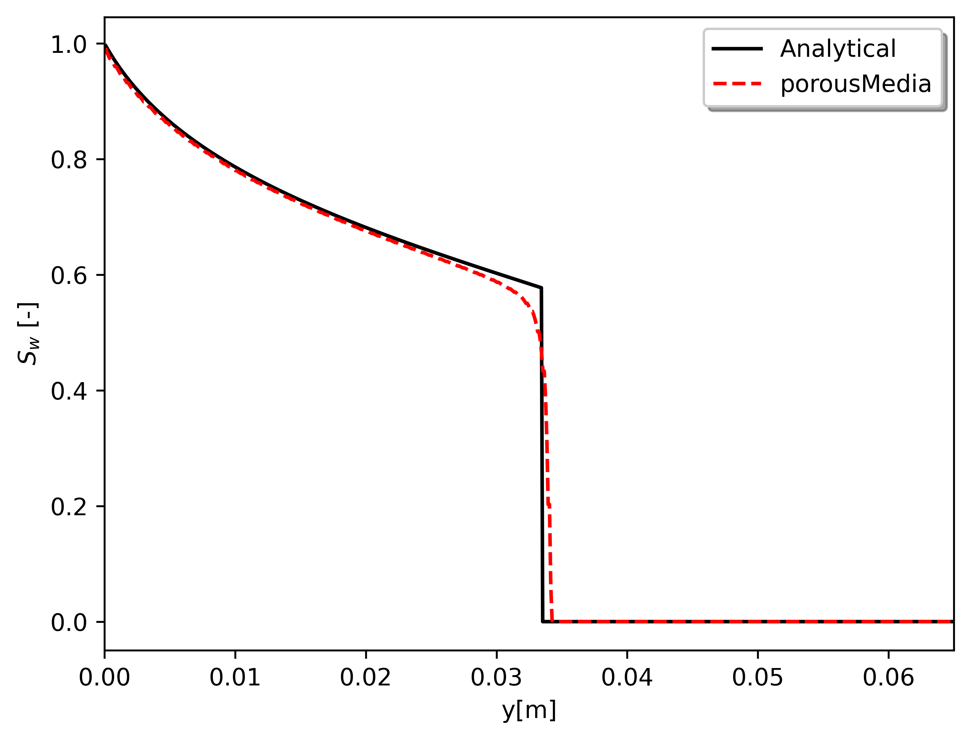
Figure 2: Saturation profile after 1800 s of the homogeneous Buckley-Leverett case.

5.1.2 Heterogeneous Buckley-Leverett

We assess the same system of the previous example, but considering a heterogeneous porosity field such that $\alpha_{v}=0.2$ if $0\leq x\leq 0.0325$, and $\alpha_{v}=0.1$ if $0.0325<x\leq 0.065$.

The saturation profile is shown in Fig. 3, where we can note a variation in the saturation curve in relation to the case of Fig. 2 due to the porosity discontinuity. For this example, the numerical solution obtained also agrees with the analytical solution.

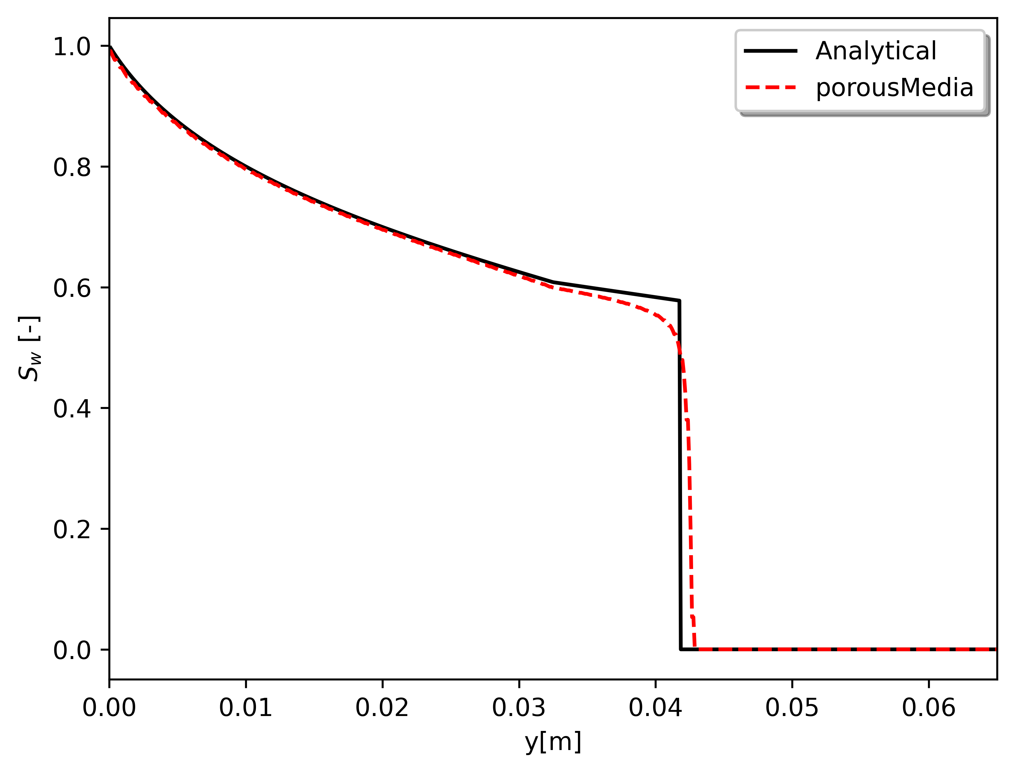
Figure 3: Saturation profile after 1800 s of the heterogeneous Buckley-Leverett case.

5.1.3 Capillary-gravity equilibrium

This example aims to evaluate the solution in the presence of gravity and capillary pressure. An air-water flow in a one meter vertical domain is carried out until the gravity-capillarity equilibrium.

The initial condition considers the lower half containing water ($S_{w}=0.5$) and air ($S_{a}=0.5$), while the upper half contains only air ($S_{w}=0$ and $S_{a}=1$). At the bottom boundary, a Neumann zero condition is applied, while the top boundary receives a Dirichlet fixed pressure of 1 MPa. Under these conditions, the water saturation at the theoretical steady state is such that:

$$\frac{\partial S_{w}}{\partial y}=\frac{(\rho_{a}-\rho_{w})g_{y}}{\frac{\partial p_{c}}{\partial S_{w}}},$$ (46)

where $g_{y}=-9.8\,\mbox{m/s}^{2}$ is the gravity acceleration [16, 20]. The capillary pressure model used is the Brooks and Corey [39], which is given by

$$p_{c}=p_{c,0}\,\left(\frac{\alpha_{i}}{\alpha_{v}}\right)^{-\beta},$$ (47)

where we set $p_{c,0}=1000$ Pa and $\beta=0.5$.

The Brooks and Corey relative permeability model with $n=3$ and $k_{r,i(\max)}=1$ is considered for both air and water. Other settings include homogeneous porosity $\alpha_{v}=0.5$, absolute permeability $\mathbf{K}=1\times 10^{-11}\,\mbox{m}^{2}$, and phase properties $\rho_{w}=1000\,\mbox{kg/m}^{3}$, $\rho_{a}=1\,\mbox{kg/m}^{3}$, $\mu_{w}=0.001\,\mbox{Pa}\cdot\mbox{s}$, and $\mu_{a}=1.76\times 10^{-5}\,\mbox{Pa}\cdot\mbox{s}$.

A final time of $115.74$ days has been chosen in order to ensure that the capillary-gravity equilibrium is attained. In this example, the time step was chosen starting at 1 s increasing by 20% until reaching 100 s. Figure 4(a) shows the water saturation profile obtained from porousMedia for a 1000 cells grid compared with the impesFoam solution for the same problem. We remark that this example is a validation case for the impesFoam solver presented in [16], where Toddy time step control is used. Note that the porousMedia and impesFoam solutions are comparable. The water saturation gradients are presented in Fig. 4(b), both in agreement with the analytical curve.

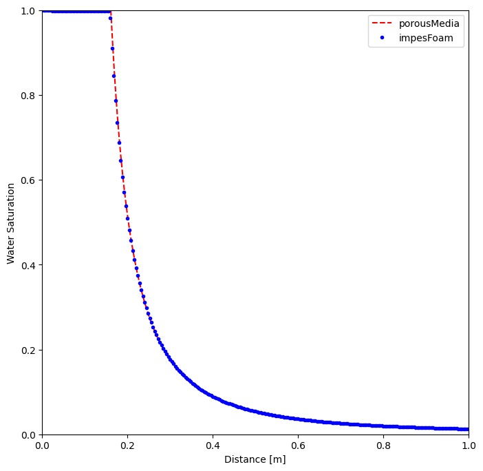
(a) Saturation profile.

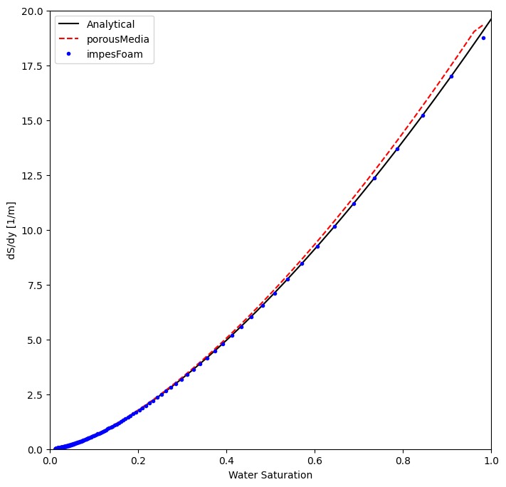
(b) Saturation gradient.

Figure 4: Capillary-gravity equilibrium test.

5.2 Stability analysis

In order to investigate the stability of the proposed method, a temporal convergence for the homogeneous Buckley-Leverett problem adding capillarity effects is presented. We consider the reference solution given by a grid with 500 computational cells and fixed time-step $\Delta t=10^{-4}$ s and study the behavior of approximations for different time refinements. The Brooks and Corey capillarity model is used with $p_{c,0}=10$ Pa and $\beta=0.5$.

When using the fully implicit strategy, the choice of time step size depends only on the accuracy request. Figure 5(a) presents the porousMedia approximations for $\Delta t=10^{-2}$ s and $\Delta t=10^{2}$ s, where it is clearly noted that the solutions are more accurate for the smaller time interval. In Fig. 5(b), we can confirm the ability of the coupledMatrixFoam solver to increase the time step when compared to the explicit method applied by the impesFoam, which has a time step restricted by the CFL (Courant-Friedrichs-Lewy) condition. Note that both solvers returned the expected linear slope, with the coupledMatrixFoam being confirmed as an excellent alternative to reduce the computational cost of simulations.

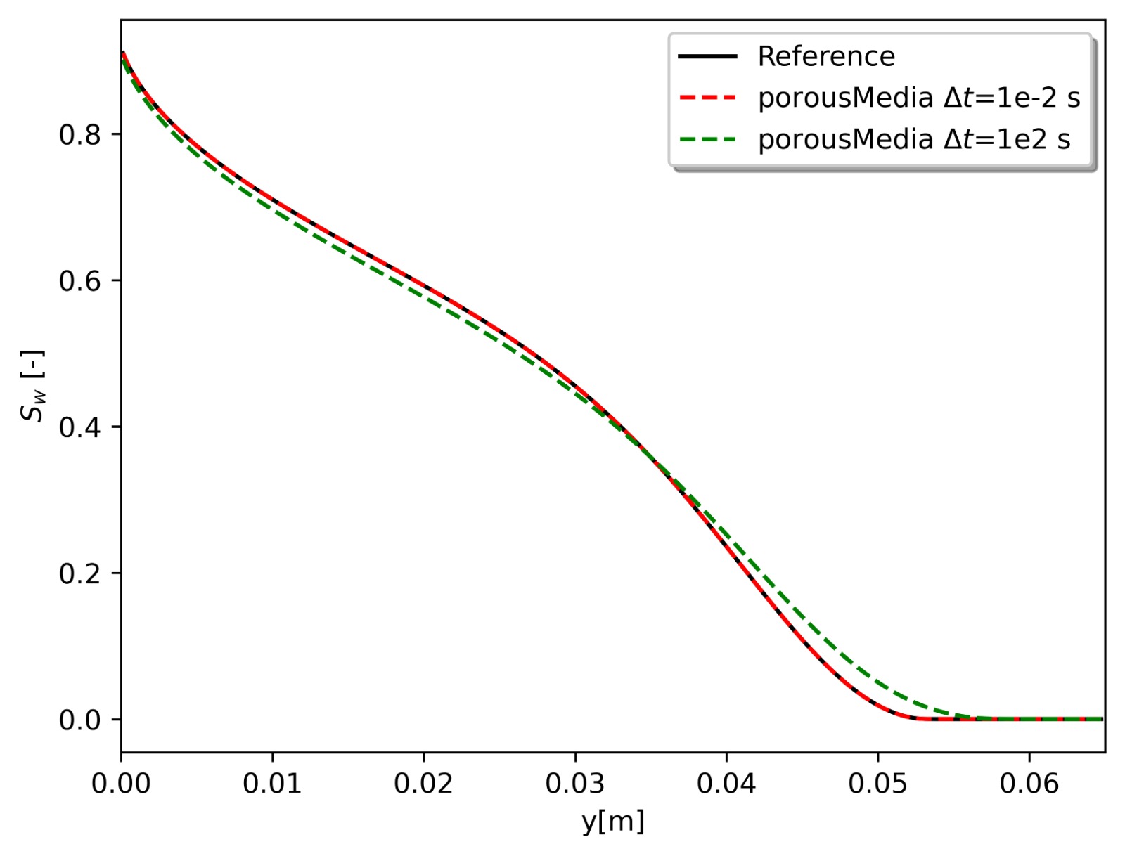
(a) Saturation profiles.

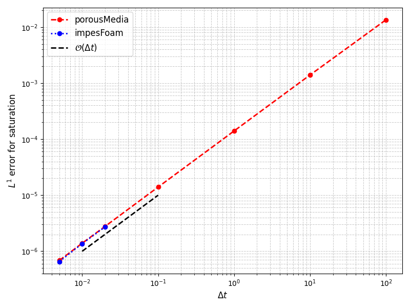
(b) $L^{1}$ errors.

Figure 5: Saturation as a function of the time step size.

5.3 Application case

The last experiment presents a simulation of an oil-water flow in a 3D heterogeneous core case, where the possibility of increasing the time step is very significant in terms of computational cost. The heterogeneous permeability field randomly generated is illustrated in Figure 6, while the porosity field is constant $\alpha_{v}=0.2$.

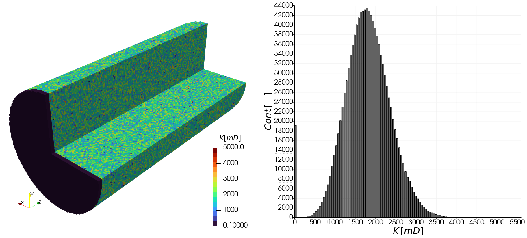
Figure 6: Randomly generated absolute permeability field.

The computational domain with 1.17 M cells distributed in $0.09\,\text{m}\times 0.09\,\text{m}\times 0.183\,\text{m}$ is initially saturated with oil and water is injected from let at a constant rate of $1.66\times 10^{-8}$m/s, with the pressure at right fixed in 101.35 MPa. The Brooks and Corey relative permeability model with $\eta=2$ and $k_{r,i(\max)}=1$ is applied for both phases, whose properties are $\rho_{w}=1000\,\mbox{kg/m}^{3}$, $\rho_{o}=800\,\mbox{kg/m}^{3}$, $\mu_{w}=0.001\,\mbox{Pa}\cdot\mbox{s}$, and $\mu_{o}=0.002\,\mbox{Pa}\cdot\mbox{s}$. We also consider the Brooks and Corey model for capillary pressure with $\beta=0.5$ and $p_{c,0}=100$ Pa, while gravity is neglected.

This application features a large mesh, so both porousMedia and impesFoam were run in parallel on a 12th Gen Intel i7-12700H CPU using six processors, as illustrated in Fig. 7. The domain decomposition was performed with the simple method, creating three partitions along the Z-axis and two along the Y-axis. No special MPI flags were applied, and the CPU did not run in exclusive mode.

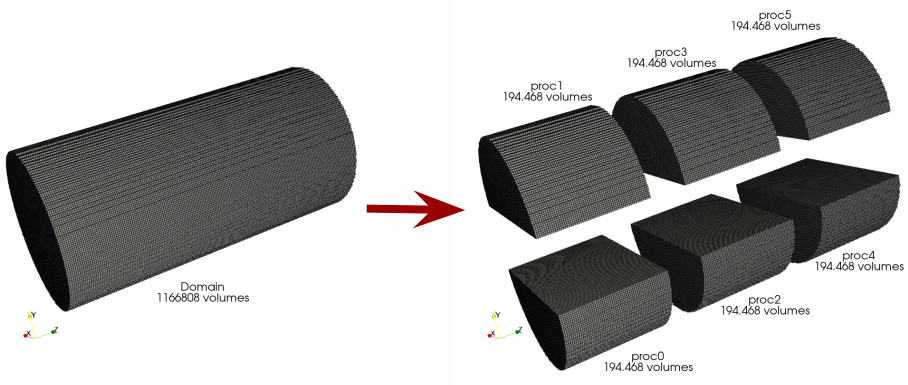
Figure 7: Domain partition scheme for parallel solution.

In this example, the effect of capillary pressure is very significant and produces a restricted time step size when using explicit methods. An adjustable time step given by Eq. (45) with $\text{Co}_{\max}=33$ has been used for the coupledMatrixFoam solver. Figure 8 illustrates the saturation solution at time $t=2$ h. The final time has been set at 50h, requiring a computational execution time of 1.49h. When running impesFoam under equivalent conditions with $\text{Co}_{\max}=0.75$, it was possible to reach 0.72 h of simulation after 13.02 h of computational execution time. Therefore, it is expected from impesFoam a running time of 904.17 h to run the equivalent final time of porousMedia. Respective time step histories are presented in Fig 9 where it is possible to observe that the time step stabilizes around 0.2 seconds for impesFoam while for the coupledMatrixFoam this stabilizes around 500 seconds. This result reinforces the ability of the implicit method to abruptly reduce the computational cost.

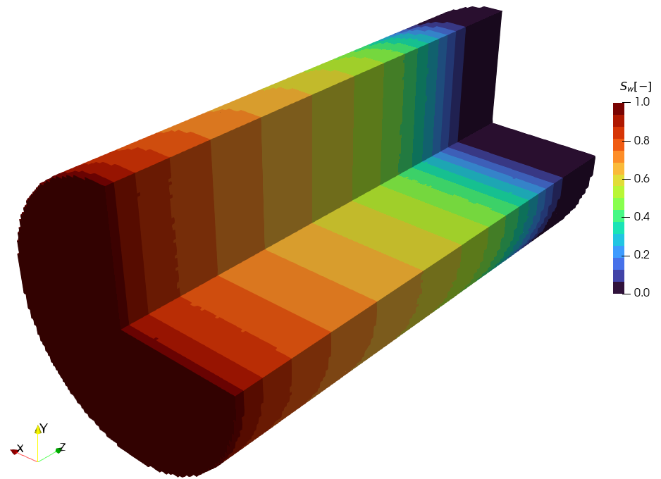
Figure 8: Saturation profile at time $t=2$ h.

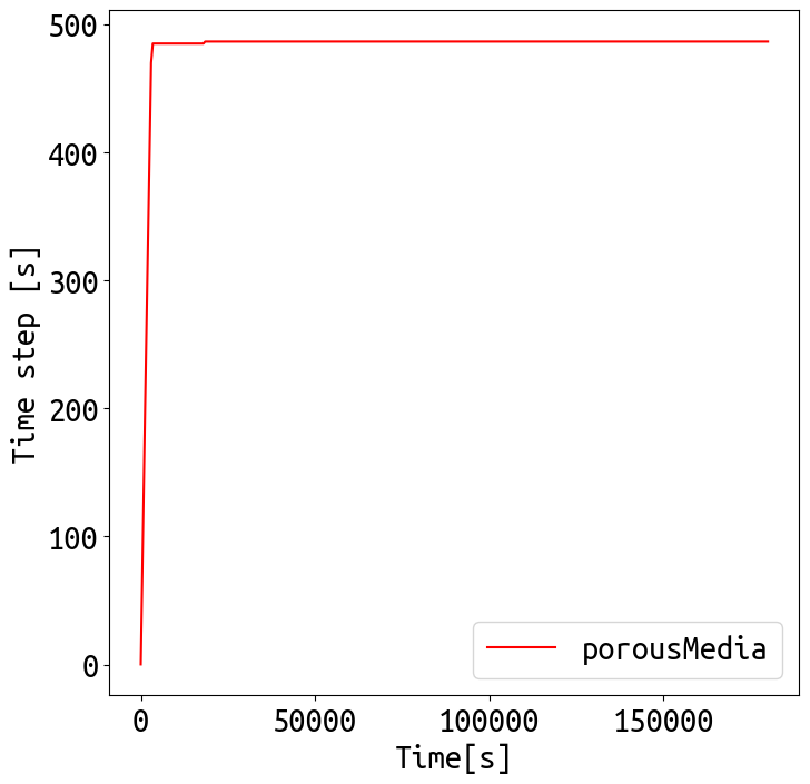
(a) CoupledMatrixFoam.

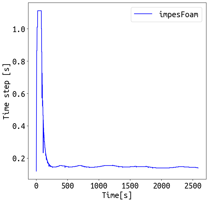
(b) impesFoam.

Figure 9: Time step histories.

5.4 Parallel performance evaluation

The CoupledMatrixFoam solver was developed with industrial applications in mind. Since such cases typically run on high-performance computing (HPC) resources, the final set of results evaluates the performance of the application case (Section 5.3) in parallel, using different processor counts.

As mentioned in Section 5.3, the baseline simulation used six processors. For the speed-up tests, an AMD EPYC 7742 CPU (64 cores) was employed in exclusive mode, without hyperthreading, scaling from a single core (serial execution) to all 64 cores. In these tests, the domain decomposition was carried out using the scotch method. To measure performance, the simulation started from a previous time of 10,000 seconds, then ran for an additional 1,000 seconds of physical time with a fixed time step of 5, seconds, resulting in 200 iterations. Furthermore, the solver was configured to perform 20 iterations of the coupled linear system every running two internal iterations.

Because the memory requirements of block-system solvers differ substantially from those of segregated solvers like impesFoam, we chose pUCoupledFoam [24] as the basis for comparison. This solver, which is natively available in foam-extend for pressure–velocity coupling, was tested using a 2D cavity tutorial case initiated from a previously converged solution. Specifically, the simulation proceeded for 20 seconds—20 iterations at a fixed time step of 1 second - on a mesh of 1,000 × 1,000 cells, yielding one million total cells. The domain decomposition was performed with the scotch method, and the block-system solver executed one internal iteration with 500 iterations per time step.

Several key differences distinguish the 2D tutorial from the main application: the latter is 3D, has about 17% more cells, and involves either three coupled variables (no reference phase) or two coupled variables (with a reference phase), whereas pUCoupledFoam couples four variables (pressure plus three velocity components). Bearing these differences in mind, the speed-up and efficiency results are presented in Figure 10.

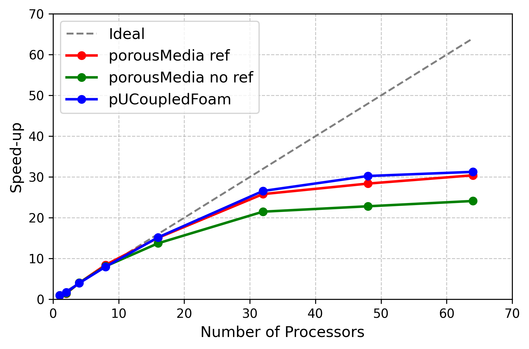
(a) Speed-up.

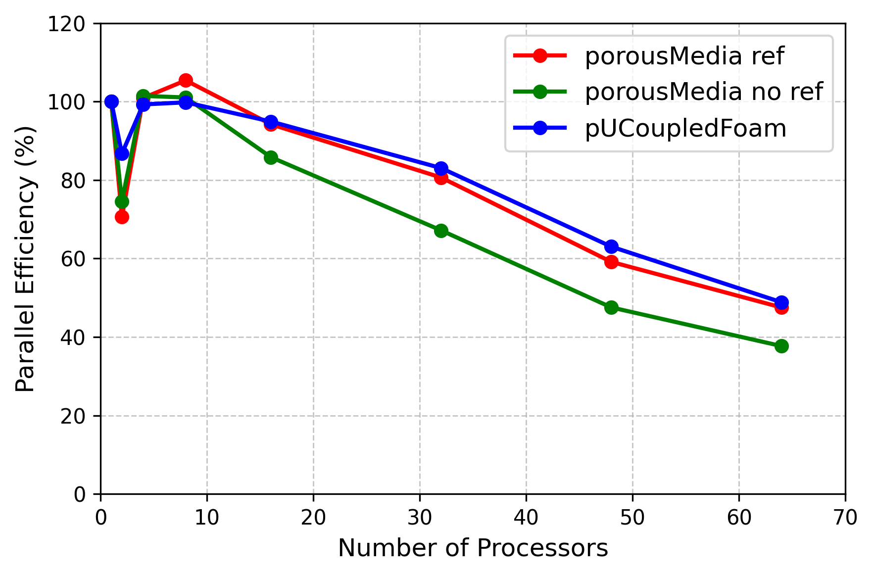
(b) Efficiency [%].

Figure 10: Comparison of performance for porousMedia with and without reference phase with pUCoupledFoam.

Figure 10(a) presents the speed-up curves for the three cases - porousMedia with (porousMedia ref) and without (porousMedia no ref) reference phase, and pUCoupledFoam - compared against the ideal linear speed-up. The ideal line represents the theoretical scenario where doubling the number of processors cuts the runtime in half. In Fig. 10(b) it is shown the parallel efficiency of the three solvers. Efficiency is computed as the ratio of actual speed-up to the ideal speed-up, expressed as a percentage. A value of 100% corresponds to perfect scaling.

Regarding the scalability of the solver, the speed-up is close to the ideal line for the three solvers until 16 processors present efficiencies higher than 80% except for the porousMedia using two processors. This behavior for two processors could be related to the difference of requirements when comparing serial and parallel simulations. Up to 16 processors the speed-up is no closer to the ideal line but it is interesting to observe that the speed-up and efficiency of porousMedia using reference phase is very close to the results of pUCoupledFoam. The behavior using more than 16 processors is expected and discussed in different works [41, 42] but without considering coupled solvers.

Finally, Figure 11 specifically compares porousMedia runtimes between the scenarios with and without a reference phase. The ratio is defined as

$$\text{ratio}=\dfrac{\text{runtime (reference phase)}}{\text{runtime (no reference phase)}}$$ (48)

and a value below 1 indicates faster execution when using a reference phase.

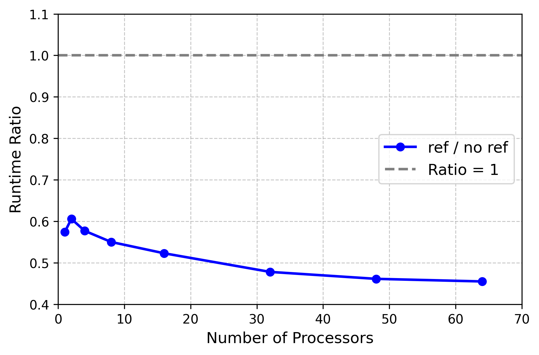
Figure 11: Runtime ratio between porousMedia using reference phase over not using.

Up to 30 processors, the runtime is less than half when the reference phase is included, with the largest ratio (approximately 0.6) observed at two processors. Effectively, removing one phase from the block system nearly doubles the solver speed, highlighting the complexity involved in analyzing block-system solver performance. Overall, these results provide a baseline for understanding how porousMedia behaves under varying configurations and computational resources.

6 Conclusion

This work introduced coupledMatrixFoam, a fully coupled, implicit solver for multiphase flows in heterogeneous porous media, developed as part of the porousMedia open-source repository maintained by WIKKI Brasil. Built on foam-extend 5.0, the solver integrates the Eulerian multi-fluid approach with Darcy’s law, allowing for the modeling of multiphase interactions in porous media with complex heterogeneous porosity and permeability fields.

By employing an implicit coupling of pressure and phase fractions, coupledMatrixFoam formulates a single block matrix system, significantly enhancing numerical stability and convergence over traditional segregated solvers. Comparative analyses with impesFoam confirmed these improvements, demonstrating a time step increase of approximately 2,500 times in a 3D heterogeneous permeability case, particularly in the presence of strong capillary pressure effects.

The solver was validated against classical Buckley-Leverett problems (homogeneous and heterogeneous cases) and a capillary-gravity equilibrium test, confirming its accuracy and reliability. Furthermore, performance evaluations on a complex 3D case demonstrated the scalability of the solver and highlighted the efficiency of the reference phase strategy, where one fluid phase is solved outside the block system to reduce computational overhead.

coupledMatrixFoam represents a significant advancement in open-source simulation tools for porous media applications, providing a robust and efficient alternative for modeling complex multiphase flow scenarios encountered in oil recovery, CO₂ sequestration, and hydrogeology. Future developments will focus on extending the solver’s capabilities to incorporate compressibility effects, reactive transport, and thermal interactions, further broadening its applicability in real-world engineering and scientific challenges.

References

- [1] J. Bear, Dynamics of fluids in porous media. Courier Corporation, 1988.
- [2] Z. Chen, G. Huan, and Y. Ma, Computational methods for multiphase flows in porous media. SIAM, 2006.
- [3] T. Koch and D. Gl “DuMux 3 - an open-source simulator for solving flow and transport problems in porous media with a focus on model coupling,” Computers & Mathematics with Applications, 2020.
- [4] S. Krogstad, K.-A. Lie, O. Møyner, H. M. Nilsen, X. Raynaud, and B. Skaflestad, “MRST-AD–an open-source framework for rapid prototyping and evaluation of reservoir simulation problems,” in SPE Reservoir Simulation Conference. Spe, 2015, p. D022S002R004.
- [5] L. Bilke, D. Naumov, W. Wang, T. Fischer, C. Lehmann, J. Buchwald, H. Shao, F. K. Kiszkurno, C. Chen, C. Silbermann, E. Radeisen, F. Zill, L. Frieder, K. Kessler, and M. Ghasabeh, “Opengeosys,” Mar. 2024. [Online]. Available: https://doi.org/10.5281/zenodo.10890088
- [6] G. E. Hammond, P. C. Lichtner, and R. T. Mills, “Evaluating the performance of parallel subsurface simulators: An illustrative example with PFLOTRAN,” Water Resources Research, vol. 50, pp. 208–228, 2014.
- [7] A. F. Rasmussen, T. H. Sandve, K. Bao, A. Lauser, J. Hove, B. Skaflestad, R. Klöfkorn, M. Blatt, A. B. Rustad, O. Sævareid et al., “The open porous media flow reservoir simulator,” Computers & Mathematics with Applications, vol. 81, pp. 159–185, 2021.
- [8] A. Wilkins, C. P. Green, and J. Ennis-King, “Porousflow: a multiphysics simulation code for coupled problems in porous media,” Journal of Open Source Software, vol. 5, no. 55, p. 2176, 2020.
- [9] H. Jasak, “Error analysis and estimation for the finite volume method with applications to fluid flows.” Ph.D. dissertation, Imperial College London (University of London), 1996.
- [10] H. G. Weller, G. Tabor, H. Jasak, and C. Fureby, “A tensorial approach to computational continuum mechanics using object-oriented techniques,” Computers in physics, vol. 12, no. 6, pp. 620–631, 1998.
- [11] S. B. Beale, H.-W. Choi, J. G. Pharoah, H. K. Roth, H. Jasak, and D. H. Jeon, “Open-source computational model of a solid oxide fuel cell,” Computer physics communications, vol. 200, pp. 15–26, 2016.
- [12] J. Maes and H. P. Menke, “GeoChemFoam: Direct modelling of multiphase reactive transport in real pore geometries with equilibrium reactions,” Transport in Porous Media, vol. 139, no. 2, pp. 271–299, 2021.
- [13] K. Missios, N. Jacobsen, K. Moeller, and J. Roenby, “Extending the isoAdvector geometric VOF method to flows in porous media,” OpenFOAM® Journal, vol. 3, pp. 66–74, 2023.
- [14] C. Soulaine, S. Pavuluri, F. Claret, and C. Tournassat, “porousMedia4Foam: Multi-scale open-source platform for hydro-geochemical simulations with OpenFOAM®,” Environmental Modelling & Software, vol. 145, p. 105199, 2021.
- [15] R. Guibert, P. Horgue, and G. Debenest, “Micro-continuum modeling of biofilm growth coupled with hydrodynamics in OpenFOAM,” SoftwareX, vol. 29, p. 102011, 2025.
- [16] P. Horgue, C. Soulaine, J. Franc, R. Guibert, and G. Debenest, “An open-source toolbox for multiphase flow in porous media,” Computer Physics Communications, vol. 187, pp. 217–226, 2015.
- [17] L. Sugumar, A. Kumar, and S. K. Govindarajan, “Grid adaptation of multiphase fluid flow solver in porous medium by OpenFOAM,” Petroleum & Coal, vol. 62, no. 4, 2020.
- [18] S. Fioroni, A. E. Larreteguy, and G. B. Savioli, “An OpenFOAM application for solving the black oil problem,” Mathematical Models and Computer Simulations, vol. 13, no. 5, pp. 907–918, 2021.
- [19] P. Horgue, F. Renard, G. S. Gerlero, R. Guibert, and G. Debenest, “porousMultiphaseFoam v2107: An open-source tool for modeling saturated/unsaturated water flows and solute transfers at watershed scale,” Computer Physics Communications, vol. 273, p. 108278, 2022.
- [20] F. J. Carrillo, I. C. Bourg, and C. Soulaine, “Multiphase flow modeling in multiscale porous media: An open-source micro-continuum approach,” Journal of Computational Physics: X, vol. 8, p. 100073, 2020.
- [21] A. Sangnimnuan, J. Li, and K. Wu, “Development of coupled two phase flow and geomechanics model to predict stress evolution in unconventional reservoirs with complex fracture geometry,” Journal of Petroleum Science and Engineering, vol. 196, p. 108072, 2021.
- [22] M. Ishii and T. Hibiki, Thermo-fluid dynamics of two-phase flow. Springer Science & Business Media, 2010.
- [23] R. Lange, G. M. Magalhães, F. F. Rocha, P. V. Coimbra, J. L. Favero, R. A. Dias, A. O. Moraes, and M. P. Schwalbert, “Development of a new computational solver for multiphase flows in heterogeneous porous media at different scales,” International Journal of Multiphase Flow, vol. 180, p. 104954, 2024.
- [24] T. Uroić, “Implicitly coupled finite volume algorithms,” Ph.D. dissertation, University of Zagreb. Faculty of Mechanical Engineering and Naval Architecture, 2019.
- [25] M. Muskat, Physical principles of oil production. IHRDC, Boston, MA, 1981.
- [26] H. G. Weller, “A new approach to VOF-based interface capturing methods for incompressible and compressible flow,” OpenCFD Ltd., Report TR/HGW, vol. 4, p. 35, 2008.
- [27] F. F. Rocha, A. H. M. Charin, G. M. Magalhães, H. R. Neto, and R. Lange, “An OpenFOAM-based multiphase solver for physical systems with stationary and moving phases using a coupled solution for phase fractions,” Proceeding Series of the Brazilian Society of Computational and Applied Mathematics, vol. 10, no. 1, pp. 2–7, 2023.
- [28] K. Coats, “IMPES stability: selection of stable timesteps,” SPE Journal, vol. 8, no. 02, pp. 181–187, 2003.
- [29] J. Monteagudo and A. Firoozabadi, “Comparison of fully implicit and impes formulations for simulation of water injection in fractured and unfractured media,” International journal for numerical methods in engineering, vol. 69, no. 4, pp. 698–728, 2007.
- [30] S. Sun, D. Keyes, and L. Liu, “Fully implicit two-phase reservoir simulation with the additive Schwarz preconditioned inexact Newton method, presented at SPE Reservoir Characterization and Simulation Conference and Exhibition,” Society of Petroleum Engineers, 2013.
- [31] H. Yang, S. Sun, Y. Li, and C. Yang, “A scalable fully implicit framework for reservoir simulation on parallel computers,” Computer Methods in Applied Mechanics and Engineering, vol. 330, pp. 334–350, 2018.
- [32] L. Luo, L. Liu, X.-C. Cai, and D. E. Keyes, “Fully implicit hybrid two-level domain decomposition algorithms for two-phase flows in porous media on 3D unstructured grids,” Journal of Computational Physics, vol. 409, p. 109312, 2020.
- [33] C. Fernandes, V. Vukčević, T. Uroić, R. Simoes, O. Carneiro, H. Jasak, and J. Nóbrega, “A coupled finite volume flow solver for the solution of incompressible viscoelastic flows,” Journal of non-newtonian fluid mechanics, vol. 265, pp. 99–115, 2019.
- [34] R. Keser, V. Vukčević, M. Battistoni, H. Im, and H. Jasak, “Implicitly coupled phase fraction equations for the Eulerian multi-fluid model,” Computers & Fluids, vol. 192, p. 104277, 2019.
- [35] R. Keser, M. Battistoni, H. G. Im, and H. Jasak, “A Eulerian multi-fluid model for high-speed evaporating sprays,” Processes, vol. 9, no. 6, p. 941, 2021.
- [36] G. G. Ferreira, P. L. Lage, L. F. L. Silva, and H. Jasak, “Implementation of an implicit pressure–velocity coupling for the Eulerian multi-fluid model,” Computers & Fluids, vol. 181, pp. 188–207, 2019.
- [37] T. Uroić and H. Jasak, “Block-selective algebraic multigrid for implicitly coupled pressure-velocity system,” Computers & fluids, vol. 167, pp. 100–110, 2018.
- [38] K. Kissling, J. Springer, H. Jasak, S. Schutz, K. Urban, and M. Piesche, “A coupled pressure based solution algorithm based on the volume-of-fluid approach for two or more immiscible fluids,” in Proceedings of the V European Conference on Computational Fluid Dynamics ECCOMAS CFD 2010, 2010.
- [39] R. H. Brooks, Hydraulic properties of porous media. Colorado State University, 1965.
- [40] Y.-S. Wu, Multiphase fluid flow in porous and fractured reservoirs. Gulf professional publishing, 2015.
- [41] F. C. C. Galeazzo, M. Garcia-Gasulla, E. Boella, J. Pocurull, S. Lesnik, H. Rusche, S. Bnà, M. Cerminara, F. Brogi, F. Marchetti, D. Gregori, R. G. Wei, and A. Ruopp, “Performance comparison of CFD microbenchmarks on diverse HPC architectures,” Computers, vol. 13, no. 5, p. 115, 2024.
- [42] F. C. C. Galeazzo, R. G. Wei, S. Lesnik, H. Rusche, and A. Ruopp, “Understanding superlinear speedup in current HPC architectures,” Preprints, vol. 2024040219, 2024.