Preconditioning without a preconditioner: faster ridge-regression and Gaussian sampling with randomized block Krylov subspace methods

Abstract

We describe a randomized variant of the block conjugate gradient method for solving a single positive-definite linear system of equations. Our method provably outperforms preconditioned conjugate gradient with a broad-class of Nyström-based preconditioners, without ever explicitly constructing a preconditioner. In analyzing our algorithm, we derive theoretical guarantees for new variants of Nyström preconditioned conjugate gradient which may be of separate interest. We also describe how our approach yields state-of-the-art algorithms for key data-science tasks such as computing the entire ridge regression regularization path and generating multiple independent samples from a high-dimensional Gaussian distribution.

1 Introduction

Solving the regularized linear system

$$\mathbf{A}_{\mu}\mathbf{x}=\mathbf{b},\quad\mathbf{A}_{\mu}:=\mathbf{A}+\mu\mathbf{I},$$ (1)

where $\mathbf{A}\in\mathbb{R}^{d\times d}$ is symmetric positive definite and $\mu\geq 0$ is a critical task across the computational sciences. Systems of the form Equation 1 arise in a variety of settings, but we are particularly motivated by two tasks in machine learning and data science: solving ridge-regression problems and sampling Gaussian vectors.

Ridge regression. Given a data matrix $\mathbf{Z}\in\mathbb{R}^{n\times d}$, a source term $\mathbf{f}\in\mathbb{R}^{n}$, and a regularization parameter $\mu\geq 0$, the ridge regression problem is

$$\min_{\mathbf{x}\in\mathbb{R}^{d}}\|\mathbf{Z}\mathbf{x}-\mathbf{f}\|^{2}+\mu\|\mathbf{x}\|^{2}.$$ (2)

A direct computation shows that the solution to Equation 2 is also the solution to

$$(\mathbf{Z}^{\mathsf{T}}\mathbf{Z}+\mu\mathbf{I})\mathbf{x}=\mathbf{Z}^{\mathsf{T}}\mathbf{f};$$ (3)

i.e. a system of the form Equation 1 with $\mathbf{A}=\mathbf{Z}^{\mathsf{T}}\mathbf{Z}$ and $\mathbf{b}=\mathbf{Z}^{\mathsf{T}}\mathbf{f}$. In a number of applications we are interested in the whole regularization path; i.e. $\mathbf{x}=\mathbf{x}_{\mu}$ for all values $\mu\geq 0$; e.g. in order to perform cross-validation to select a value of $\mu$ to use for future predictions.

Sampling Gaussians. If $\mathbf{b}$ has independent standard normal entries, then $\bm{\mu}+\mathbf{A}^{1/2}\mathbf{b}$ is a Gaussian vector with mean $\bm{\mu}$ and covariance $\mathbf{A}$. In order to approximate $\mathbf{A}^{1/2}\mathbf{b}$, it is common to make use of the identity

$$\mathbf{A}^{1/2}\mathbf{b}=\frac{2}{\pi}\int_{0}^{\infty}\mathbf{A}(\mathbf{A}+z^{2}\mathbf{I})^{-1}\mathbf{b}\,\mathrm{d}z.$$ (4)

The term $(\mathbf{A}+z^{2}\mathbf{I})^{-1}\mathbf{b}$ in the integrand of Equation 4 is of the form Equation 1 with $\mu=z^{2}$. Often we are interested in sampling several Gaussian vectors with the same covariance matrix.

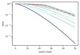
Figure 1: Comparison of the convergence (in terms of matrix-loads) of our proposed randomized variant of the block conjugate gradient method () against standard conjugate gradient () and the state of the art Nyström preconditioned conjugate gradient (Frangella et al., 2023) with various choices of hyperparameters (). Our method outperforms these existing methods without the need for selecting hyperparameters, which may be difficult to do effectively in practice (see Theorem 3.2).

1.1 Computational assumptions

Throughout this paper, we assume $\mathbf{A}$ is accessed only through matrix-vector products $\mathbf{x}\mapsto\mathbf{A}\mathbf{x}$ or block matrix-vector products $[\mathbf{x}_{1}~\cdots~\mathbf{x}_{m}]\mapsto[\mathbf{A}\mathbf{x}_{1}~\cdots~\mathbf{A}\mathbf{x}_{m}]$. While one can simulate a block matrix-vector product using $m$ matrix-vector products, the parallelism inherent in modern computing architectures means the cost of block products is often nearly independent of the block size $m$ (so long as $m$ is not too large). Allowing for more efficient data-access is widely understood as one of the major benefits of many randomized linear algebra algorithms (Halko et al., 2011; Li et al., 2017; Tropp & Webber, 2023).

The algorithms we propose in this paper are designed to economize the number of times $\mathbf{A}$ is loaded into memory (henceforth referred to as matrix-loads), and not other costs such as matrix-vector products or storage. In settings where matrix-loads are not the dominant cost, the proposed algorithms may not yield significant advantages. The costs of the algorithm are discussed more in Section 3.2, and we explore them in the numerical experiments in Section 5.

1.2 Notation

We denote the eigenvalues of $\mathbf{A}$ by $\lambda_{1}\geq\cdots\geq\lambda_{d}$ and of those of an arbitrary positive definite matrix $\mathbf{M}$ by $\lambda_{1}(\mathbf{M})\geq\cdots\geq\lambda_{d}(\mathbf{M})$. The condition number of $\mathbf{M}$ is $\kappa(\mathbf{M}):=\lambda_{1}(\mathbf{M})/\lambda_{d}(\mathbf{M})$ and the spectral norm is $\|\mathbf{M}\|:=\lambda_{1}(\mathbf{B})$. The $\mathbf{M}$-norm of a vector $\mathbf{x}$ is $\|\mathbf{x}\|_{\mathbf{M}}:=\|\mathbf{M}^{1/2}\mathbf{x}\|=\sqrt{\mathbf{x}^{\mathsf{T}}\mathbf{M}\mathbf{x}}$.

1.3 Organization

In Section 2 we describe key background on Krylov subspace methods and preconditioning. Our algorithm and main theoretical results are described in Section 3 and proved in Section 4. Numerical experiments are provided in Section 5. Finally show how the theory we develop can be used to sample Gaussian vectors in Section 6.

2 Background

Krylov Subspace Methods (KSM) make use of the Krylov subspace

$$\mathcal{K}_{t}(\mathbf{A},\mathbf{b}):=\operatorname{span}\{\mathbf{b},\mathbf{A}\mathbf{b},\ldots,\mathbf{A}^{t-1}\mathbf{b}\},$$ (5)

and are perhaps the most widely used algorithms for solving systems of the form Equation 1. The methods we discuss in this section are standard, and for mathematical simplicity, we define them by their optimality conditions rather than algorithmically. We discuss implementation details in Appendix A; see also (Greenbaum, 1997; Saad, 2003; Meurant, 2006) for comprehensive treatments of these methods.

2.1 Preconditioned Conjugate Gradient

The preconditioned conjugate gradient algorithm (PCG) is perhaps the most powerful KSM for positive edfinite linear systems. PCG makes use of a positive definite preconditioner $\mathbf{P}_{\mu}$ that transforms the system $\mathbf{A}_{\mu}\mathbf{x}=\mathbf{b}$ into the system

$$(\mathbf{P}_{\mu}^{-1/2}\mathbf{A}_{\mu}\mathbf{P}_{\mu}^{-1/2})\mathbf{y}=\mathbf{P}_{\mu}^{-1/2}\mathbf{b},\quad\mathbf{P}_{\mu}^{1/2}\mathbf{x}=\mathbf{y},$$ (6)

and works over a transformed Krylov subspace

$$\mathcal{K}_{t}(\mathbf{A}_{\mu},\mathbf{b};\mathbf{P}_{\mu}):=\mathcal{K}_{t}(\mathbf{P}_{\mu}^{-1}\mathbf{A},\mathbf{P}_{\mu}^{-1}\mathbf{b}).$$ (7)

Specifically, PCG is defined defined by an optimality condition.

Definition 2.1.

The $t$-th PCG iterate corresponding to a positive definite preconditioner $\mathbf{P}_{\mu}$ is defined as

$$\mathsf{pcg}_{t}(\mu):=\operatornamewithlimits{argmin}_{\mathbf{x}\in\mathcal{K}_{t}(\mathbf{A}_{\mu},\mathbf{b};\mathbf{P}_{\mu})}\|\mathbf{A}_{\mu}^{-1}\mathbf{b}-\mathbf{x}\|_{\mathbf{A}_{\mu}}.$$

The iterate $\mathsf{pcg}_{t}(\mu)$ can be computed using $t-1$ matrix-vector products with $\mathbf{A}$ (and $t$ products with $\mathbf{P}_{\mu}^{-1}$). We discuss implementation details in Appendix A.

The simplest choice of preconditioner is $\mathbf{P}_{\mu}=\mathbf{I}$, which yields the standard conjugate gradient algorithm (CG) (Hestenes & Stiefel, 1952).

Definition 2.2.

The $t$-th CG iterate is defined as

$$\mathsf{cg}_{t}(\mu):=\operatornamewithlimits{argmin}_{\mathbf{x}\in\mathcal{K}_{t}(\mathbf{A},\mathbf{b})}\|\mathbf{A}_{\mu}^{-1}\mathbf{b}-\mathbf{x}\|_{\mathbf{A}_{\mu}}.$$

2.1.1 Convergence

PCG (and hence CG) satisfy a well-known convergence guarantee in terms of the condition number of the preconditioned system $\mathbf{P}_{\mu}^{-1/2}\mathbf{A}_{\mu}\mathbf{P}_{\mu}^{-1/2}$; see e.g. (Greenbaum, 1997).

Corollary 2.3.

Let $\mathbf{P}_{\mu}$ be any preconditioner and let

$$\varepsilon_{t}(\mu):=2\exp\left(-\frac{2t}{\sqrt{\kappa(\mathbf{P}_{\mu}^{-1/2}\mathbf{A}_{\mu}\mathbf{P}_{\mu}^{-1/2})}}\right).$$

Then the $t$-th preconditioned-CG iterate corresponding to the preconditioner $\mathbf{P}_{\mu}$ satisfies

$$\frac{\|\mathbf{A}_{\mu}^{-1}\mathbf{b}-\mathsf{pcg}_{t}(\mu)\|_{\mathbf{A}_{\mu}}}{\|\mathbf{A}_{\mu}^{-1}\mathbf{b}\|_{\mathbf{A}_{\mu}}}\leq\varepsilon_{t}(\mu).$$

Corollary 2.3 implies that if we can find $\mathbf{P}_{\mu}$ so that $\kappa(\mathbf{P}_{\mu}^{-1/2}\mathbf{A}_{\mu}\mathbf{P}_{\mu}^{-1/2})$ is small, then PCG converges rapidly. The choice of $\mathbf{P}_{\mu}$ minimizing this condition number is of course $\mathbf{P}_{\mu}=\mathbf{A}_{\mu}^{-1}$, but this is not a practical preconditioner; if we knew $\mathbf{A}_{\mu}^{-1}$ we could easily compute the solution $\mathbf{A}_{\mu}^{-1}\mathbf{b}$. Thus, finding a suitable choice of $\mathbf{P}_{\mu}$, which balances improvements to the convergence of PCG with the cost of building/applying $\mathbf{P}_{\mu}$ is critical.

2.2 Deflation preconditioner

If $\mathbf{A}$ is poorly conditioned due to the presence of $r$ eigenvalues much larger than the remaining $n-r$ eigenvalues, then we might hope to learn a good approximation of the top $r$ eigenvalues and “correct” this ill-conditioning. Towards this end, suppose we have a good rank-$r$ approximation $\mathbf{U}\mathbf{D}\mathbf{U}^{\mathsf{T}}$ to $\mathbf{A}$, where $\mathbf{U}$ has orthonormal columns and $\mathbf{D}$ is diagonal. Intuitively, this low-rank approximation contains the information needed to remove the top eigenvalues of $\mathbf{A}$, thereby reducing the condition number of the preconditioned system. In particular, one can form the preconditioner

$$\mathbf{P}_{\mu}:=\frac{1}{\theta+\mu}\mathbf{U}(\mathbf{D}+\mu\mathbf{I})\mathbf{U}^{\mathsf{T}}+(\mathbf{I}-\mathbf{U}\mathbf{U}^{\mathsf{T}}),$$ (8)

and it is not hard to verify that

$$\mathbf{P}_{\mu}^{-1}=(\theta+\mu)\mathbf{U}(\mathbf{D}+\mu\mathbf{I})^{-1}\mathbf{U}^{\mathsf{T}}+(\mathbf{I}-\mathbf{U}\mathbf{U}^{\mathsf{T}}).$$ (9)

Here $\theta>0$ is a parameter that must be chosen along with the factorization $\mathbf{U}\mathbf{D}\mathbf{U}^{\mathsf{T}}$.

Applying $\mathbf{P}_{\mu}^{-1}$ to a vector requires $O(dr)$ arithmetic operations, which is relatively cheap if $r\ll d$. Hence, so long as a reasonable factorization $\mathbf{U}\mathbf{D}\mathbf{U}^{\mathsf{T}}$ can be obtained, Equation 8 can be used as a preconditioner; see (Frank & Vuik, 2001; Gutknecht, 2012) and the references within.

2.2.1 Exact deflation

Traditionally, it has been suggested to take $\mathbf{U}\mathbf{D}\mathbf{U}^{\mathsf{T}}$ as $[\![\mathbf{A}]\!]_{r}$, the best rank-$r$ approximation to $\mathbf{A}$; i.e. to set $\mathbf{D}$ as the top $r$ eigenvalues of $\mathbf{A}$ and $\mathbf{U}$ the corresponding eigenvectors. In this case Equation 8 is sometimes called a spectral deflation preconditioner. The name arises because the eigenvalues of $\mathbf{P}_{\mu}^{-1/2}\mathbf{A}_{\mu}\mathbf{P}_{\mu}^{-1/2}$ are

$$\underbrace{\theta+\mu,\ldots,\theta+\mu}_{\text{$r$-copies}},\lambda_{r+1}+\mu,\ldots,\lambda_{d}+\mu,$$ (10)

and hence, if $\theta\in[\lambda_{d},\lambda_{r+1}]$, then the condition number of $\mathbf{P}_{\mu}^{-1/2}\mathbf{A}_{\mu}\mathbf{P}_{\mu}^{-1/2}$ is $(\lambda_{r+1}+\mu)/(\lambda_{d}+\mu)$. In other words, the top $r$ eigenvalues of $\mathbf{A}_{\mu}$ are deflated. In combination with Corollary 2.3, this yields the following convergence guarantee.

Corollary 2.4.

Let $\mathbf{P}_{\mu}$ be the preconditioner Equation 8 corresponding to $[\![\mathbf{A}]\!]_{r}$, the rank-$r$ truncated SVD of $\mathbf{A}$, and $\theta\in[\lambda_{d},\lambda_{r+1}]$ and let

$$\varepsilon_{t}(\mu):=2\exp\left(-\frac{2t}{\sqrt{(\lambda_{r+1}+\mu)/(\lambda_{d}+\mu)}}\right).$$

Then the $t$-th PCG iterate (Definition 2.1) corresponding to the preconditioner $\mathbf{P}_{\mu}$ satisfies

$$\frac{\|\mathbf{A}_{\mu}^{-1}\mathbf{b}-\mathsf{pcg}_{t}(\mu)\|_{\mathbf{A}_{\mu}}}{\|\mathbf{A}_{\mu}^{-1}\mathbf{b}\|_{\mathbf{A}_{\mu}}}\leq\varepsilon_{t}(\mu).$$

When $\lambda_{r+1}\ll\lambda_{1}$ and $\mu$ is not too large, then the rate of convergence guaranteed by the bound can be much faster than without preconditioning ($r=0$). Of course, any potential benefits to convergence must be weighted against the cost of constructing the spectral deflation preconditioner, and exact deflation, which requires computing the top eigenvectors of $\mathbf{A}$, can be costly.

2.2.2 Nyström preconditioning

Techniques from randomized numerical linear algebra allow near-optimal low-rank approximations to $\mathbf{A}$ to be computed very efficiently (Halko et al., 2011; Tropp & Webber, 2023). Intuitively, we might hope that the the corresponding preconditioner works nearly as well as spectral deflation.

In particular, it’s reasonable to take $\mathbf{U}\mathbf{D}\mathbf{U}^{\mathsf{T}}$ as the eigendecomposition of the Nyström approximation

$$\mathbf{A}\langle\mathbf{K}_{s}\rangle:=(\mathbf{A}\mathbf{K}_{s})(\mathbf{K}_{s}^{\mathsf{T}}\mathbf{A}\mathbf{K}_{s})^{\dagger}(\mathbf{K}_{s}^{\mathsf{T}}\mathbf{A}),$$ (11)

where $\mathbf{\Omega}\in\mathbb{R}^{d\times\ell}$ is a matrix of independent standard normal random variables and

$$\mathbf{K}_{s}:=[\mathbf{\Omega}~\mathbf{A}\mathbf{\Omega}~\cdots~\mathbf{A}^{s-1}\mathbf{\Omega}]\in\mathbb{R}^{d\times(s\ell)}.$$ (12)

This variant of the Nyström approximation is among the most powerful randomized low-rank approximation algorithms, and can be implemented using $s$ matrix-loads (Tropp & Webber, 2023).

Nyström-based preconditioning has proven effective in theory and practice, and has been an active area of research in recent years (Martinsson & Tropp, 2020; Frangella et al., 2023; Carson & Daužickaitė, 2024; Díaz et al., 2023; Zhao et al., 2024; Dereziński et al., 2025).

Most related to the content of this paper is the theoretical analysis of (Frangella et al., 2023), which proves that if $s=1$, $\theta=\lambda_{\ell}(\mathbf{A}\langle\mathbf{\Omega}\rangle)$, and the sketching dimension $\ell$ is on the order of the effective dimension

$$d_{\textup{eff}}(\mu):=\operatorname{tr}\bigl{(}\mathbf{A}\mathbf{A}_{\mu}^{-1}\bigr{)}=\sum_{i=1}^{d}\frac{\lambda_{i}}{\lambda_{i}+\mu},$$ (13)

then Nyström PCG converges in at most $t=O(\log(1/\varepsilon))$ iterations; i.e. independent of any spectral properties of $\mathbf{A}$. Our analysis makes use of the same general techniques as (Frangella et al., 2023), but is applicable when $s>1$ as well as if $\mu=0$. We discuss the theoretical bounds of (Frangella et al., 2023) as well as some possible shortcomings of using bounds based on the effective dimension in Section D.2.

3 Our approach: augmented block-CG

In this paper, we advocate for the use of block-KSMs for solving Equation 1. Given a matrix $\mathbf{B}\in\mathbb{R}^{d\times m}$ (typically $m\ll d$) with columns $\mathbf{b}^{(1)},\ldots,\mathbf{b}^{(m)}$, the block Krylov subspace is

$$\mathcal{K}_{t}(\mathbf{A},\mathbf{B}):=\mathcal{K}_{t}(\mathbf{A},\mathbf{b}^{(1)})+\cdots+\mathcal{K}_{t}(\mathbf{A},\mathbf{b}^{(m)}).$$ (14)

That is, $\mathcal{K}_{t}(\mathbf{A},\mathbf{B})$ is the space consisting of all linear combinations of vectors in $\mathcal{K}_{t}(\mathbf{A},\mathbf{b}^{(1)}),\ldots,\mathcal{K}_{t}(\mathbf{A},\mathbf{b}^{(m)})$.

This naturally gives rise to the block-CG algorithm (O’Leary, 1980).

Definition 3.1.

Let $\mathbf{B}=[\mathbf{b}^{(1)}~\cdots~\mathbf{b}^{(m)}]$. The $t$-th block-CG iterates are defined as

$$\mathsf{bcg}_{t}^{(i)}(\mu):=\operatornamewithlimits{argmin}_{\mathbf{x}\in\mathcal{K}_{t}(\mathbf{A},\mathbf{B})}\|\mathbf{A}_{\mu}^{-1}\mathbf{b}^{(i)}-\mathbf{x}\|_{\mathbf{A}_{\mu}}.$$ (15)

The block-CG iterates $\mathsf{bcg}_{t}^{(1)}(\mu),\ldots,\mathsf{bcg}_{t}^{(m)}(\mu)$ can be simultaneously computed using $t-1$ block matrix-vector products with $\mathbf{A}$. We discuss implementation and costs further in Section 3.2.

3.1 Main theoretical results

Our first main result is the observation that by augmenting $\mathbf{b}$ with $\mathbf{\Omega}$, block-CG implicitly enjoys the benefits of certain classes of preconditioners built using $\mathbf{\Omega}$. In particular, we have the following error guarantee:

Theorem 3.2.

Fix any matrix $\mathbf{\Omega}\in\mathbb{R}^{d\times m}$ and let $\mathbf{P}=(\mathbf{I}+\mathbf{X})^{-1}$ be any preconditioner where $\operatorname{range}(\mathbf{X})\subseteq\mathcal{K}_{s+1}(\mathbf{A},\mathbf{\Omega})$. Define the augmented starting block $\mathbf{B}=[\mathbf{b}~\mathbf{\Omega}]$. Then, for any $t\geq s$, the $t$-th block-CG iterate is related to the $(t-s)$-th preconditioned-CG iterate corresponding to the preconditioner $\mathbf{P}_{\mu}$ in that

$$\|\mathbf{A}_{\mu}^{-1}\mathbf{b}-\mathsf{bcg}_{t}^{(1)}(\mu)\|_{\mathbf{A}_{\mu}}\leq\|\mathbf{A}_{\mu}^{-1}\mathbf{b}-\mathsf{pcg}_{t-s}(\mu)\|_{\mathbf{A}_{\mu}}.$$

In particular, when $\mathbf{U}\mathbf{D}\mathbf{U}^{\mathsf{T}}=\mathbf{A}\langle\mathbf{K}_{s}\rangle$, then the deflation preconditioner $\mathbf{P}_{\mu}$ defined in Equation 8 has the form

$$\mathbf{P}^{-1}=\mathbf{I}+\mathbf{X},\text{where $\operatorname{range}(\mathbf{X})\subseteq\mathcal{K}_{s}(\mathbf{A},\mathbf{\Omega})$}.$$ (16)

Remark 3.3.

Theorem 3.2 asserts that augmented block-CG automatically performs no worse than Nyström PCG (with the best choice of $s$ and $\theta$) after the same number of matrix-loads. This explains the performance observed in Figure 1.

We use Theorem 3.2, and a new bound for Nyström preconditioning (Theorem 4.4), to prove a bound for block-CG reminiscent of Corollary 2.4 for the spectral deflation preconditioner.

Corollary 3.4.

Let $\mathbf{\Omega}\in\mathbb{R}^{d\times(r+2)q}$, where $q\geq\log(1/\delta)/\log(100)$, be a random Gaussian matrix and define the augmented starting block $\mathbf{B}=[\mathbf{b}~\mathbf{\Omega}]$. Let

$$\varepsilon_{t}(\mu):=2\exp\left(-\frac{t-(3+\log(d))}{3\sqrt{(\lambda_{r+1}+\mu)/(\lambda_{d}+\mu)}}\right).$$

Then the block-CG satisfies, with probability at least $1-\delta$,

$$\Bigg{\{}\forall\mu\geq 0:\frac{\|\mathbf{A}_{\mu}^{-1}\mathbf{b}-\mathsf{bcg}_{t}^{(1)}(\mu)\|_{\mathbf{A}_{\mu}}}{\|\mathbf{A}_{\mu}^{-1}\mathbf{b}\|_{\mathbf{A}_{\mu}}}\leq\varepsilon_{t}(\mu)\Bigg{\}}.$$

In particular, after a small burn-in period of $O(\log(d))$ iterations, we have exponential convergence at a rate roughly $\sqrt{(\lambda_{r+1}+\mu)/(\lambda_{d}+\mu)}$. Corollary 3.4 is a special case of a more general bound Theorem 4.5 which takes into account the eigenvalue decay of $\mathbf{A}$.

Remark 3.5.

The fact that Corollary 3.4 guarantees an accurate result for all $\mu\geq 0$ with high probability (as opposed to a single value of $\mu$) will be important in our applications. In particular, it allows guarantees for computing the whole ridge-regression regularization path and will be necessary in the analysis of our algorithm for sampling Gaussian vectors.

Remark 3.6.

Bounds based on the condition number (such as Corollary 3.4) are often pessimistic in practice. To determine how many iterations to run, it is more common to use some sort of a posteriori error estimate. For example, observing the residual $\|\mathbf{b}-\mathbf{A}_{\mu}\mathsf{bcg}_{t}^{(1)}(\mu)\|$ gives some indication of the quality of the solution. More advanced techniques can also be used (Meurant & Tichý, 2024).

3.2 Computational costs

The block-CG method is a standard algorithm in numerical analysis, and there are many mathematically equivalent implementations; i.e. different implementations which produce the same output in exact arithmetic. Here we describe a block-Lanczos based implementation of block-CG that is particularly suitable for our applications to ridge regression and Gaussian sampling.

The block-Lanczos algorithm (which we describe explicitly in Appendix A) applied to $(\mathbf{A},\mathbf{B})$ for $t$ iterations produces $\mathbf{Q}_{t}$ with orthonormal columns and $\mathbf{T}_{t}$ with bandwidth $2m+1$ satisfying

$$\operatorname{range}(\mathbf{Q}_{t})=\mathcal{K}_{t}(\mathbf{A},\mathbf{B}),\quad\mathbf{Q}_{t}^{\mathsf{T}}\mathbf{A}\mathbf{Q}_{t}=\mathbf{T}_{t}.$$ (17)

A standard computation (see Appendix B) reveals that

$$\mathsf{bcg}_{k}^{(1)}(\mu)=\|\mathbf{b}\|\mathbf{Q}_{t}(\mathbf{T}_{t}+\mu\mathbf{I})^{-1}\mathbf{e}_{1},$$ (18)

where $\mathbf{e}_{1}=[1,0,\ldots,0]^{\mathsf{T}}$. In particular, since $\mathcal{K}_{t}(\mathbf{A}_{\mu},\mathbf{B})=\mathcal{K}_{t}(\mathbf{A},\mathbf{B})$ for any scalar $\mu$, Equation 18 can be used to compute the block-CG iterate for multiple values of $\mu$ using the same $\mathbf{Q}_{t}$ and $\mathbf{T}_{t}$.

Theorem 3.7.

Suppose $\mathbf{B}\in\mathbb{R}^{d\times m}$. The block-Lanczos algorithm applied to $(\mathbf{A},\mathbf{B})$ for $t$ iterations produces $\mathbf{Q}_{t}$ and $\mathbf{T}_{t}$ using:

• $t-1$ matrix-loads of $\mathbf{A}$ (for a total of $m(t-1)$ total matrix-products)

• $O(dm^{2}t^{2})$ floating point operations operations, and

• $O(dmt)$ storage.

Subsequently, for any $\mu\geq 0$, the $t$-th block-CG iterates $\mathsf{bcg}_{t}^{(1)}(\mu)$, can be computed using an additional $O(dmt+m^{3}t)$ floating point operations operations.

We emphasize that after the block Lanczos algorithm has been run, the cost to compute the block-CG iterates for multiple values of $\mu$ is relatively small. This is in contrast to Nyström PCG, which is is not particularly well suited for solving Equation 1 for multiple values of $\mu$; while the Nyström approximation can be reused, PCG must be re-run and new products with $\mathbf{A}$ computed.

3.3 Comparison with past work

The block-CG algorithm is widely used to solve linear systems with multiple right hand sides, and in such settings working over the block Krylov subspace is often advantageous compared to working over the individual Krylov subspaces (O’Leary, 1980; Meurant, 1984; Feng et al., 1995; Birk & Frommer, 2013). To the best of our knowledge, ours is the first work to consider a randomized variant of the block-CG algorithm as well as the first to prove that block-CG can outperform standard CG, even with the goal of solving a single linear system.

More broadly, a number of recent works in randomized numerical linear algebra (Chen & Hallman, 2023; Tropp & Webber, 2023; Meyer et al., 2024) have made use of various nestedness properties of block-KSMs similar in flavor to Theorem 4.1 in order to obtain more efficient algorithms.

4 Main analysis

In this section we give our theoretical analysis of augmented block-CG. In light of Theorem 3.2, our main strategy for deriving bounds for block-CG is simply to derive bounds for Nyström PCG. We do not attempt to optimize constants, opting instead for simple arguments and clean theorem statements.

4.1 Implicit preconditioning with block KSMs

We begin with a key observation.

Theorem 4.1.

Suppose $\mathbf{P}_{\mu}=(\mathbf{I}+\mathbf{X})^{-1}$ for some $\mathbf{X}$ with $\operatorname{range}(\mathbf{X})\subseteq\mathcal{K}_{s+1}(\mathbf{A}_{\mu},\mathbf{\Omega})$. Then,

$$\mathcal{K}_{t}(\mathbf{A}_{\mu},\mathbf{b};\mathbf{P}_{\mu})\subseteq\mathcal{K}_{t}(\mathbf{A},\mathbf{b})+\mathcal{K}_{t+s}(\mathbf{A},\mathbf{\Omega}).$$

A full proof is contained in Section B.1, but the basic idea is simple. By definition, $\mathcal{K}_{t}(\mathbf{A}_{\mu},\mathbf{b};\mathbf{P}_{\mu})$ consists linear combinations of the vectors

$$(\mathbf{P}_{\mu}^{-1}\mathbf{A})^{k}\mathbf{P}_{\mu}^{-1}\mathbf{b}=((\mathbf{I}+\mathbf{X})\mathbf{A})^{k}(\mathbf{I}+\mathbf{X})\mathbf{b},$$ (19)

where $k=0,1,\ldots,t-1$. And each $((\mathbf{I}+\mathbf{X})\mathbf{A})^{k}(\mathbf{I}+\mathbf{X})\mathbf{b}$ can be expressed as linear combination of vectors which live in the specificed space.

Proof of Theorem 3.2.

Clearly $\mathcal{K}_{t}(\mathbf{A},\mathbf{b})+\mathcal{K}_{t+s}(\mathbf{A},\mathbf{\Omega})\subseteq\mathcal{K}_{t+s}(\mathbf{A},[\mathbf{b}~\mathbf{\Omega}])$, so the result follows immediately from Theorem 4.1 and the optimality of block-CG and preconditioned-CG. ∎

4.2 Bounds for Nyström preconditioning

We begin by recalling a error guarantee for Nyström low-rank approximation, which compares the Nyström error $\|\mathbf{A}-\mathbf{A}\langle\mathbf{K}_{s}\rangle\|$ to the error $\|\mathbf{A}-[\![\mathbf{A}]\!]_{r}\|=\lambda_{r+1}$ of the best possible rank-$r$ approximation to $\mathbf{A}$.

Theorem 4.2 (Theorem 9.1 in (Tropp & Webber, 2023)).

Suppose $\mathbf{\Omega}\in\mathbb{R}^{d\times(r+p)}$ is a random Gaussian matrix and define

$$\mathbf{K}_{s}:=[\mathbf{\Omega}~\mathbf{A}\mathbf{\Omega}~\cdots~\mathbf{A}^{s-1}\mathbf{\Omega}].$$ (20)

Then, if $p\geq 2$,

$$\log\Biggl{(}\frac{\operatorname{\mathbb{E}}\|\mathbf{A}-\mathbf{A}\langle\mathbf{K}_{s}\rangle\|^{2}}{\lambda_{r+1}^{2}}\Bigg{)}$$

$$\hskip 30.00005pt\leq\frac{1}{8(s-\frac{3}{2})^{2}}\log\Biggl{(}4+\frac{4r}{p-1}\sum_{i>r}\frac{\lambda_{i}^{2}}{\lambda_{r+1}^{2}}\Bigg{)}^{2}.$$

The other main result that we need is a deterministic bound for the condition number of the Nyström preconditioned system, similar to Proposition 5.3 in (Frangella et al., 2023). The proof, which is contained in Appendix B, follows the exact same approach, although we state the bound for arbitrary $\theta>0$ while (Frangella et al., 2023) states it for one particular choice.

Theorem 4.3.

Let $\mathbf{P}_{\mu}$ be the Nyström preconditioner Equation 8 corresponding to the Nyström approximation $\mathbf{A}\langle\mathbf{K}\rangle$ for any $\mathbf{K}$ and shift parameter $\theta\geq 0$. Then

$$\kappa(\mathbf{P}_{\mu}^{-1/2}\mathbf{A}_{\mu}\mathbf{P}_{\mu}^{-1/2})$$

$$\hskip 20.00003pt\leq\big{(}\theta+\mu+\|\mathbf{A}-\mathbf{A}\langle\mathbf{K}\rangle\|\big{)}\left(\frac{1}{\theta+\mu}+\frac{1}{\lambda_{d}+\mu}\right).$$

To prove our main convergence guarantee for our augmented block-CG, we derive a new bound for Nyström preconditioning.

Theorem 4.4.

Let $\mathbf{\Omega}\in\mathbb{R}^{d\times(r+p)}$ be a random Gaussian matrix and define

$$\mathbf{K}_{s}:=[\mathbf{\Omega}~\mathbf{A}\mathbf{\Omega}~\cdots\mathbf{A}^{s-1}\mathbf{\Omega}].$$ (21)

Let $\mathbf{P}_{\mu}$ be the Nyström preconditioner Equation 8 corresponding to the Nyström approximation $\mathbf{A}\langle\mathbf{K}_{s}\rangle$ for any shift parameter $\theta\in[\lambda_{d},\lambda_{r+1}]$.

Suppose $p\geq 2$ and

$$s\geq\frac{3}{2}+\frac{1}{2}\log\left(4+\frac{4r}{p-1}\sum_{i>r}\frac{\lambda_{i}^{2}}{\lambda_{r+1}^{2}}\right).$$

Then, with probability at least $99/100$,

$$\bigg{\{}\forall\mu:\kappa(\mathbf{P}_{\mu}^{-1/2}\mathbf{A}_{\mu}\mathbf{P}_{\mu}^{-1/2})\leq 28\frac{\lambda_{r+1}(\mathbf{A})+\mu}{\lambda_{d}+\mu}\bigg{\}}.$$

Theorem 4.4, which we prove in Section B.2, follows from Theorems 4.2 and 4.3 and a simple application of Markov’s inequality. Our bound for Nyström PCG applies even when $\mu=0$, whereas the bounds in (Frangella et al., 2023) require $\mu$ to be sufficiently large relative to the sketching dimension $r+p$ and consider only $s=1$.

Theorem 4.4 may be hard for users of Nyström PCG to instantiate, since it is stated in terms of the (unknown) eigenvalues of $\mathbf{A}$. If $p=2$ then

$$s\geq 3+\log(d)$$ (22)

is sufficient to guarantee the condition on $s$. However, the user must still guarantee $\theta\in[\lambda_{d},\lambda_{r+1}]$, and different choices may lead to better or worse convergence. Theorem 3.2 implies that choosing $\theta$ is uneccessary for our augmented block-CG method.

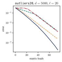
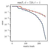
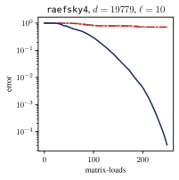
Figure 2: Error versus matrix-loads for block-CG (), CG (), and Nyström PCG with $s=1$ () and $s=3$ () on several test problems.

4.3 Bounds for augmented block-CG

We can now state our main convergence guarantee for augmented block-CG. This result is a simple consequence of our condition number bound Theorem 4.4 and the error guarantee Corollary 2.3 for PCG.

Theorem 4.5.

Let $\mathbf{\Omega}\in\mathbb{R}^{d\times(r+p)q}$, where $q\geq\log(1/\delta)/\log(100)$, be a random Gaussian matrix. Suppose that $p\geq 2$,

$$s\geq\frac{5}{2}+\frac{1}{4}\log\left(4+\frac{4r}{p-1}\sum_{i>r}\frac{\lambda_{i}^{2}}{\lambda_{r+1}^{2}}\right),$$

and

$$\varepsilon_{t}(\mu):=2\exp\left(-\frac{t-s}{\sqrt{(\lambda_{r+1}+\mu)/(\lambda_{d}+\mu)}}\right).$$

Then, the block-CG iterate $\mathsf{bcg}_{t}^{(1)}(\mu)$ satisfies, with probability at least $1-\delta$,

$$\Bigg{\{}\forall\mu:\frac{\|\mathbf{A}_{\mu}^{-1}\mathbf{b}-\mathsf{bcg}_{t}^{(1)}(\mu)\|_{\mathbf{A}_{\mu}}}{\|\mathbf{A}_{\mu}^{-1}\mathbf{b}\|_{\mathbf{A}_{\mu}}}\leq\varepsilon_{t}(\mu)\Bigg{\}}.$$

Proof of Corollary 3.4.

Set $p=2$ and $s\geq 3+\log(d)$. By Equation 22 we can instantiate Theorem 4.5. ∎

4.4 Can increasing the Nyström depth parameter help?

As noted in Remark 3.3, our main result Theorem 3.2 allows us to compare augmented block-CG to Nyström PCG for a range of low-rank approximation depths $s$. Unfortuantely, standard bounds for randomized KSMs for low-rank approximation are for “large-block” methods which use a block size $\ell$ comparable to the target rank $r$ (Halko et al., 2011; Musco & Musco, 2015; Tropp & Webber, 2023). As a result, our bounds for Nyström preconditioning (e.g. Theorems 4.4 and 4.5) do not improve substantially as $s$ increases, and so there is no benefit in “optimizing” over $s$.

Note that $\mathbf{A}\langle\mathbf{K}_{s}\rangle$ as defined in Equation 11 can have rank as large as $\ell s$. Therefore, we might hope that it is competitive with the best rank-$\ell s$ approximation to $\mathbf{A}$; i.e. that

$$\|\mathbf{A}-\mathbf{A}\langle\mathbf{K}_{s}\rangle\|\approx\lambda_{\ell s+1}.$$ (23)

While this is not always possible (e.g. if $\mathbf{A}$ had many repeated top eigenvalues), recent work (Meyer et al., 2024) proves that for rank-$r$ approximation, certain “small-block” KSMs (e.g. with $\ell=O(1)$) can perform nearly as well as “large-block” KSMs (e.g. with $\ell=O(r)$) in terms of matrix-products under mild assumptions on eigenvalue gaps. Extending the ideas of (Meyer et al., 2024) to the Nyström approximation Equation 11 would immediately provide better results for Nyström PCG and hence our augmented block-CG.

5 Numerical experiments

We use the block-Lanczos algorithm with full-reorthogonalization in order to implement block-CG and the block-Lanczos square root iterates. Implementation details are described in Appendix A. The $s$ matrix-loads required to build the Nyström preconditioner are accounted for in the plots. We use the same random Gaussian matrix $\mathbf{\Omega}\in\mathbb{R}^{d\times\ell}$ for Nyström PCG and block-CG. More numerical experiments, including without full-reorthogonalization, are included in Appendix E.

5.1 Convergence

We begin by comparing the convergence of the methods discussed in this paper on several test problems. The results of this experiment are illustrated in Figure 2, and as expected, our augmented block-CG method outperforms the other methods, often by orders-of-magnitude. We also observe that Nyström PCG benefits from using $s>1$; i.e. from performing more than one passes over $\mathbf{A}$ when building the preconditioner.

As discussed in Section 1.1, throughout this paper we assume that matrix-loads (iterations) are the dominant cost. For reference, we have also show convergence as a function of matrix-vector products in Figure 9.

5.2 Regularization parameter

In Figure 3 we plot the error after a fixed number of matrix loads as a function of $\mu$. As expected, this plot indicates that our augmented block-CG outperforms the other methods for each value of $\mu$.

Perhaps more importantly, our block-CG method can efficiently compute the solution to Equation 1 for many values of $\mu$, without the need for additional matrix-load (see Theorem 3.7). This is in contrast to Nyström PCG which requires a new run for each value of $\mu$. For tasks such as ridge regression, this is of note.

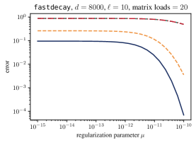
Figure 3: Error after a fixed number of matrix-loads as a function of the regularization parameter $\mu$ for block-CG (), CG (), and Nyström PCG with $s=1$ () and $s=3$ ().

6 Gaussian sampling

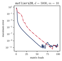
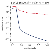
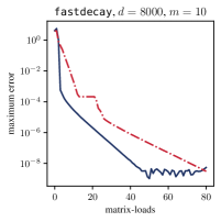
Figure 4: Maximum sample error versus matrix-loads for Lanczos square root () and block-Lanczos square root ().

Several applications in data science and statistics require sampling Gaussians with a given mean and covariance (Thompson, 1933; Besag et al., 1991; Bardsley, 2012; Wang & Jegelka, 2017). A standard approach is to transform an isotropic Gaussian vector. Indeed, suppose $\mathbf{b}\sim\mathcal{N}(\mathbf{0},\mathbf{I})$ (i.e. that entries of $\mathbf{b}$ are independent standard Gaussians). Then, for positive definite $\mathbf{A}$,

$$\bm{\mu}+\mathbf{A}^{1/2}\mathbf{b}\sim\mathcal{N}(\bm{\mu},\mathbf{A}).$$ (24)

In other words, in order to sample Gaussian vectors with covariance $\mathbf{A}$, it suffices to apply the matrix-square root of $\mathbf{A}$ to a standard Gaussian vector and then shift this result by $\bm{\mu}$. The most computationally difficult part of this is applying the square root of $\mathbf{A}$ to $\mathbf{b}$.

Recall the expression Equation 4:

$$\mathbf{A}^{1/2}\mathbf{b}=\frac{2}{\pi}\int_{0}^{\infty}\mathbf{A}(\mathbf{A}+z^{2}\mathbf{I})^{-1}\mathbf{b}\,\mathrm{d}z.$$ Equation 4

When $t$ is sufficiently large, we might hope that $\mathsf{cg}_{t}(z^{2})\approx(\mathbf{A}+z^{2}\mathbf{I})^{-1}\mathbf{b}$. This motivates the following definition.

Definition 6.1.

The $t$-th Lanczos square root iteration is defined as

$$\mathsf{sq}_{t}:=\frac{2}{\pi}\int_{0}^{\infty}\mathbf{A}\mathsf{cg}_{t}(z^{2})\,\mathrm{d}z.$$

This and closely related methods appear throughout the literature (Chow & Saad, 2014; Pleiss et al., 2020; Chen, 2024).

Often we wish to sample multiple vectors from $\mathcal{N}(\bm{\mu},\mathbf{A})$, and so we might use a block-variant of Definition 6.1.

Definition 6.2.

Let $\mathbf{B}=[\mathbf{b}^{(1)}~\cdots~\mathbf{b}^{(m)}]$. The $t$-th block-Lanczos square root iterate is defined as

$$\mathsf{bsq}_{t}^{(i)}:=\frac{2}{\pi}\int_{0}^{\infty}\mathbf{A}\mathsf{bcg}_{t}^{(i)}(z^{2})\,\mathrm{d}z.$$

Both algorithms can be efficiently implemented using the (block)-Lanczos algorithms; see Section C.3.

Using our analysis of augmented block-CG we are able to prove the following convergence guarantee.

Theorem 6.3.

Let $\mathbf{b}^{(1)},\ldots,\mathbf{b}^{(m)}\in\mathbb{R}^{d}$ be independent standard Gaussian random vectors. Suppose

$$r\leq(m-1)\left\lceil\frac{\log(m/\delta)}{\log(100)}\right\rceil^{-1}-2,$$

$C=\log(16\lambda_{1}/\lambda_{d})$, and

$$\varepsilon_{t}:=C\exp\left(-\frac{t-(3+\log(d))}{3\sqrt{(\lambda_{r+1}+\mu)/(\lambda_{d}+\mu)}}\right)$$

Then, with probability at least $1-\delta$,

$$\Bigg{\{}\forall i:\frac{\|\mathbf{A}^{1/2}\mathbf{b}^{(i)}-\mathsf{bsq}_{t}^{(i)}\|}{\|\mathbf{A}^{1/2}\|\|\mathbf{b}^{(i)}\|}\leq\varepsilon_{t}\Bigg{\}}.$$

The proof is contained in Appendix C and basically amounts to integrating Corollary 3.4. In particular, when sampling $m$ Gaussians, $\mathbf{b}^{(1)},\ldots,\mathbf{b}^{(m)}$ are independent isotropic Gaussian vectors. Therefore, $[\mathbf{b}^{(2)},\ldots,\mathbf{b}^{(m)}]$ is a Gaussian matrix independent of $\mathbf{b}^{(1)}$, and hence $\mathsf{bcg}_{t}^{(1)}(z^{2})$ will enjoy the benefits of augmented block-CG described in this paper. Thus, we expect $\mathsf{bsq}_{t}^{(1)}(z^{2})$ to converges more quickly the larger $m$ is. Critically, since $\mathsf{bsq}_{t}^{(i)}(z^{2})$ are identically distributed, this acceleration is also enjoyed by $\mathsf{bsq}_{t}^{(i)}(z^{2})$ for all $i$, without the need to generate any new random vectors!

Thus, block-Lanczos square root method allows us to sample $m$ Gaussians with roughly

$$m\Big{(}\log(d)+\sqrt{\lambda_{r+1}/\lambda_{d}}\log\big{(}\log(\lambda_{1}/\lambda_{d})/\varepsilon\big{)}\Big{)}$$ (25)

matrix-vector products, where $r=O(m/\log(m))$. In contrast, existing bounds for methods like the single-vector Lanczos square root method Definition 6.1 (Chen et al., 2022; Pleiss et al., 2020) sample a single Gaussian vector with roughly $\sqrt{\lambda_{1}/\lambda_{d}}\log(1/\varepsilon)$ matrix-vector products. Therefore, when $\lambda_{r+1}\ll\lambda_{1}$, the total number of matrix-vector products is reduced significantly by using the block method in Definition 6.2.

6.1 Numerical experiments

We perform an experiment comparing the block-Lanczos square root iterate to the standard Lanczos square root iterate. In particular, in Figure 4, we compare the maximum error in approximating $\mathbf{A}^{1/2}\mathbf{b}^{(i)}$, $i=1,\ldots,m$ for the two methods. All runs of the single-vector method are done in parallel so that the number of matrix-loads is independent of $m$. The block method outperforms the single-vector method, and the performance gains are often significant.

7 Outlook

We have introduced a variant of the block-CG method which outperforms Nyström PCG, both in theory and in practice. Our work is perhaps the first to provide theoretical evidence of the virtues of block Krylov subspace methods for solving a single linear system of equations and sampling Gaussian vectors. There is significant potential to derive better theory and algorithms for such methods, particularly by developing a better understanding of randomized low-rank approximation (Meyer et al., 2024).

In order to derive our theoretical bounds we describe new variants of Nyström PCG that use a block-Krylov Nyström approximation and prove theoretical guarantees for these variants. Our theory and numerical experiments suggest that these methods perform better than the simple Nyström approximation suggested in (Frangella et al., 2023).

Finally, it would be interesting to understand the extend to which similar ideas can be extended to other tasks involving matrix-functions, such as estimating the trace of matrix-functions. Existing algorithms often involve applying matrix-functions to many Gaussian vectors (Ubaru et al., 2017; Epperly et al., 2024; Meyer et al., 2024), so it seems likely that using block-Krylov methods may be advantageous to using single-vector methods. However, existing theory does not reflect this.

Impact Statement

This paper presents work whose goal is to advance the field of Machine Learning. There are many potential societal consequences of our work, none which we feel must be specifically highlighted here.

Disclaimer

This paper was prepared for informational purposes by the Global Technology Applied Research center of JPMorgan Chase & Co. This paper is not a merchandisable/sellable product of the Research Department of JPMorgan Chase & Co. or its affiliates. Neither JPMorgan Chase & Co. nor any of its affiliates makes any explicit or implied representation or warranty and none of them accept any liability in connection with this paper, including, without limitation, with respect to the completeness, accuracy, or reliability of the information contained herein and the potential legal, compliance, tax, or accounting effects thereof. This document is not intended as investment research or investment advice, or as a recommendation, offer, or solicitation for the purchase or sale of any security, financial instrument, financial product or service, or to be used in any way for evaluating the merits of participating in any transaction.

Appendix A Implementation and pseudocode

We describe an implementation of Definition 3.1 based on the block-Lanczos algorithm, which produces a matrix $\mathbf{Q}_{t}$ whose columns form an orthonormal basis for $\mathcal{K}_{t}(\mathbf{A},\mathbf{B})$. A basic version of the block Lanczos algorithm is described in Algorithm 1.

Algorithm 1 Block Lanczos

1: Input: $\mathbf{A}$, $\mathbf{B}$, $t$

2: $\hat{\mathbf{Q}}_{0},\hat{\mathbf{B}}_{-1}=\textsc{QR}(\mathbf{B})$, $\hat{\mathbf{Q}}_{-1}=\mathbf{0}$

3: for $n=0,1,\ldots,t-1$ do

4:  $\mathbf{Y}_{n+1}=\mathbf{A}\hat{\mathbf{Q}}_{n}-\mathbf{Q}_{n-1}\hat{\mathbf{B}}_{n-1}^{\mathsf{T}}$

5:  $\hat{\mathbf{A}}_{n}=\hat{\mathbf{Q}}_{n}^{\mathsf{T}}\mathbf{Y}_{n+1}$

6:  $\mathbf{Z}_{n+1}=\mathbf{Y}_{n+1}-\hat{\mathbf{Q}}_{n}\mathbf{A}_{n}$

7:  for $j=0,1,\ldots,n$ do

8:   $\mathbf{Z}_{n+1}=\mathbf{Z}_{n+1}-\hat{\mathbf{Q}}_{j}(\hat{\mathbf{Q}}_{j}^{\mathsf{T}}\mathbf{Z}_{n+1})$

9:  end for

10:  $\hat{\mathbf{Q}}_{n+1},\hat{\mathbf{B}}_{n}=\textsc{QR}(\mathbf{Z}_{n+1})$

11: end for

12: Output: $\{\hat{\mathbf{Q}}_{n}\}$, $\{\hat{\mathbf{A}}_{n}\}$, $\{\hat{\mathbf{B}}_{n}\}$

Note that in line 10 the QR factorization may require deflation if $\mathbf{Z}_{n+1}$ is rank-deficient.

Assuming the algorithm terminates successfully, the output satisfies a symmetric three term recurrence

$$\mathbf{A}\hat{\mathbf{Q}}_{n}=\hat{\mathbf{Q}}_{n-1}\hat{\mathbf{B}}_{n-1}^{\mathsf{T}}+\hat{\mathbf{Q}}_{n}\hat{\mathbf{A}}_{n}+\hat{\mathbf{Q}}_{n+1}\hat{\mathbf{B}}_{n}.$$ (26)

We obtain the matrix $\mathbf{Q}_{t}$ by assembling the Lanczos basis matrices

$$\mathbf{Q}_{t}:=\begin{bmatrix}|&|&&|\\ \hat{\mathbf{Q}}_{0}&\hat{\mathbf{Q}}_{1}&\cdots&\hat{\mathbf{Q}}_{t-1}\\ |&|&&|\\ \end{bmatrix}.$$ (27)

Similarly, we obtain a matrix $\mathbf{T}_{t}$ by

$$\mathbf{T}_{t}:=\begin{bmatrix}\hat{\mathbf{A}}_{0}&\hat{\mathbf{B}}_{0}^{\mathsf{T}}\\ \hat{\mathbf{B}}_{0}&\hat{\mathbf{A}}_{1}&\ddots&\phantom{\ddots}\\ &\ddots&\ddots&\hat{\mathbf{B}}_{t-2}^{\mathsf{T}}\\ &&\hat{\mathbf{B}}_{t-2}&\hat{\mathbf{A}}_{t-1}\\ \end{bmatrix}.$$ (28)

Here the $\hat{\mathbf{B}}_{n}$ are upper triangular, so $\mathbf{T}_{t}$ has total bandwidth $2m+1$.

The Krylov basis $\mathbf{Q}_{t}$ and the coefficient matrix $\mathbf{T}_{t}$ are related by Equation 26 which can be written as

$$\mathbf{A}\mathbf{Q}_{t}=\mathbf{Q}_{t}\mathbf{T}_{t}+\hat{\mathbf{Q}}_{t}\hat{\mathbf{B}}_{t-1}\mathbf{E}_{t}^{\mathsf{T}},$$ (29)

where $\mathbf{E}_{t}$ is the $(mt)\times m$ matrix with the $m\times m$ identity in the last $m$ rows and zeros elsewhere.

The output of the block-Lanczos algorithm can be used to efficiently compute the block-CG iterates.

Theorem A.1.

Let $\mathsf{bcg}_{t}(\mu):=[\mathsf{bcg}_{t}^{(1)}(\mu)~\cdots~\mathsf{bcg}_{t}^{(m)}(\mu)]$. Then

$$\mathsf{bcg}_{t}(\mu)=\mathbf{Q}_{t}(\mathbf{T}_{t}+\mu\mathbf{I})^{-1}\mathbf{E}_{1}\hat{\mathbf{B}}_{-1},$$ (30)

where $\mathbf{E}_{1}$ is the $(mt)\times m$ matrix with the $m\times m$ identity in the first $m$ rows and zeros elsewhere.

Proof.

For any matrix $\mathbf{K}$,

$$\mathbf{K}(\mathbf{K}^{\mathsf{T}}\mathbf{A}_{\mu}\mathbf{K})^{-1}\mathbf{K}^{\mathsf{T}}\mathbf{b}=\operatornamewithlimits{argmin}_{\mathbf{x}\in\operatorname{range}(\mathbf{K})}\|\mathbf{A}_{\mu}^{-1}\mathbf{b}-\mathbf{x}\|_{\mathbf{A}_{\mu}}.$$ (31)

Indeed, observe that any $\mathbf{x}\operatorname{range}(\mathbf{K})$ has the form $\mathbf{x}=\mathbf{K}\mathbf{c}$. By direct computation,

$$\hskip-10.00002pt\operatornamewithlimits{argmin}_{\mathbf{c}}\|\mathbf{A}_{\mu}^{-1}\mathbf{b}-\mathbf{K}\mathbf{c}\|_{\mathbf{A}_{\mu}}$$ (32)

$$=\operatornamewithlimits{argmin}_{\mathbf{c}}\|\mathbf{A}_{\mu}^{-1/2}\mathbf{b}-\mathbf{A}_{\mu}^{1/2}\mathbf{K}\mathbf{c}\|_{2}$$ (33)

$$=((\mathbf{A}_{\mu}^{1/2}\mathbf{K})^{\mathsf{T}}(\mathbf{A}_{\mu}^{1/2}\mathbf{K}))^{-1}(\mathbf{A}_{\mu}^{1/2}\mathbf{K})^{\mathsf{T}}(\mathbf{A}_{\mu}^{-1/2}\mathbf{b})$$ (34)

$$=(\mathbf{K}^{\mathsf{T}}\mathbf{A}_{\mu}\mathbf{K})^{-1}\mathbf{K}^{\mathsf{T}}\mathbf{b}.$$ (35)

This proves Equation 31.

Therefore, by Equation 17, we see that

$$\mathsf{bcg}_{t}(\mu)=\mathbf{Q}_{t}(\mathbf{T}_{t}+\mu\mathbf{I})^{-1}\mathbf{Q}_{t}^{\mathsf{T}}\mathbf{B}.$$ (36)

We get the final result by noting that $\mathbf{B}=\hat{\mathbf{Q}}_{0}\hat{\mathbf{B}}_{-1}$ and $\mathbf{Q}_{t}^{\mathsf{T}}\hat{\mathbf{Q}}_{0}=\mathbf{E}_{1}$. ∎

The special case in Equation 18 is a consequence of the fact that $\hat{\mathbf{B}}_{-1}$ is obtained as the “R” factor of the QR factorization of $\mathbf{B}$. In particular, the first column is zero except the top entry of $\hat{\mathbf{B}}_{-1}$ which is $\|\mathbf{b}\|$.

Proof of Theorem 3.7.

At each iteration the block-Lanczos algorithm (Algorithm 1) performs one matrix-load ($m$ parallel matrix products) and lower-order arithmetic dominated by the reorthogonalization costs, in which $\mathbf{Z}_{n+1}$ is orthgonalized against all of the previous $\hat{\mathbf{Q}}_{j}$. Each product $\hat{\mathbf{Q}}_{j}(\hat{\mathbf{Q}}_{j}^{\mathsf{T}}\mathbf{Z}_{n+1})$ costs $O(dm^{2})$ operations, and there are $n$ total products. This is done for iterations $n=0,\ldots,t-1$, resulting in a total arithmetic cost $O(dm^{2}t^{2})$.

Since $\mathbf{T}_{t}$ (and hence $\mathbf{T}_{t}+\mu\mathbf{I}$) are $(mt)\times(mt)$ matrices of bandwidth $O(m)$, the linear system $(\mathbf{T}_{t}+\mu\mathbf{I})\mathbf{z}=\mathbf{e}_{1}$ can be solved in $O((mt)m^{2})=O(m^{3}t)$ time. Subsequently, since $\mathbf{Q}_{t}$ is a $d\times(mt)$ matrix, $\mathbf{Q}_{t}\mathbf{z}$ can be computed in $O(dmt)$ time. ∎

In exact arithmetic, it is in fact possible to reduce the floating point cost to $O(dmtL+m^{3}tL)$ and the storage to $O(dm+dL)$, where $L$ is the number of values of $\mu$ at which one wishes to evaluate $\mathsf{bcg}_{t}^{(1)}(\mu)$ (O’Leary, 1980). However, there are several caveats to such an implementation. First, such methods require knowing the values of $\mu$ at which one wishes to evaluate $\mathsf{bcg}_{t}^{(1)}(\mu)$ ahead of time. Second, the finite-precision behavior of such methods can differ greatly from the exact arithmetic behavior. We discuss the impacts of finite precision arithmetic in Section A.1, and in Appendix E we perform some numerical experiments that indicate that reorthogonalization may be unnecessary in some situations.

A.1 Finite precision arithmetic

It is well-known that the behavior of KSMs in finite precision arithmetic may be very different from exact arithmetic (Greenbaum, 1997; Meurant, 2006).

In exact arithmetic, lines 7 and 8 of Algorithm 1 are unnecessary as $\mathbf{Z}_{n+1}$ will already be orthogonal to the existing Krylov subspace. Omitting these lines reduces the arithmetic costs, and also allows the previous columns of the block Krylov subspace to be processed and discarded as they are generated, thereby reducing storage costs as well. In finite precision arithmetic, omitting reorthogonalization can have a major impact. In particular, the columns of $\mathbf{Q}_{t}$ can lose orthogonality (and even linear independence).

For methods based on the standard Lanczos algorithm (Algorithm 1 with block size one), there is quite a bit of theory which guarantees that such methods can still work, even without orthogonalization (Paige, 1971, 1976; Druskin & Knizhnerman, 1991; Greenbaum, 1989; Musco et al., 2018; Chen, 2024).

Unfortunately, much less theory is known about the block-Lanczos algorithm in finite precision arithmetic. In fact, even with reorthogonalization, the behavior of the block-Lanczos algorithm is more much more complicated than the standard Lanczos algorithm. For instance, the QR factorization in line 10 must do some sort of deflation if $\mathbf{Z}_{n+1}$ is (numerically) rank-deficient.

Without reorthogonalization, we observe that in many cases the block-CG method fails to converge at all, while in other cases it does converge for some time; see Appendix E. Understanding this behavior is well beyond the scope of the current work.

Appendix B Omitted proofs

In this section, we provide proofs that were omitted in the main text.

B.1 Nestendness

We begin by proving that the Krylov subspace used by PCG, for certain types of preconditioners, is contained in a certain block-Krylov subspace.

Proof of Theorem 4.1.

Since (block) Krylov subspaces are shift invariant, without loss of generality it suffices to consider the case $\mu=0$. For notational simplicity we will denote $\mathbf{P}_{\mu}$ by $\mathbf{P}$.

We proceed by induction, beginning with the base case $t=1$. Observe that,

$$\mathcal{K}_{1}(\mathbf{P}^{-1}\mathbf{A},\mathbf{P}^{-1}\mathbf{b}) =\operatorname{span}(\mathbf{P}^{-1}\mathbf{b})$$ (37)

$$=\operatorname{span}((\mathbf{I}+\mathbf{X})\mathbf{b})$$ (38)

$$=\operatorname{span}(\mathbf{b}+\mathbf{X}\mathbf{b}).$$ (39)

Clearly $\mathbf{b}\in\mathcal{K}_{1}(\mathbf{A},\mathbf{b})$ and $\mathbf{X}\mathbf{b}\in\operatorname{range}(\mathbf{X})\subseteq\mathcal{K}_{s+1}(\mathbf{A},\mathbf{\Omega})$, so $\mathbf{\mathbf{b}+\mathbf{X}\mathbf{b}}\subseteq\mathcal{K}_{1}(\mathbf{A},\mathbf{b})+\mathcal{K}_{s+t}(\mathbf{A},\mathbf{\Omega})$ as desired.

Now, assume that

$$\mathcal{K}_{t-1}(\mathbf{P}^{-1}\mathbf{A},\mathbf{P}^{-1}\mathbf{b}) \subseteq\mathcal{K}_{t-1}(\mathbf{A},\mathbf{b})+\mathcal{K}_{(t-1)+s}(\mathbf{A},\mathbf{\Omega}).$$

Now we consider the order $t$ subspace

$$\mathcal{K}_{t}(\mathbf{P}^{-1}\mathbf{A},\mathbf{P}^{-1}\mathbf{b})=\operatorname{span}\{\mathbf{P}^{-1}\mathbf{b},(\mathbf{P}^{-1}\mathbf{A})\mathbf{P}^{-1}\mathbf{b},\ldots,$$

$$\hskip 50.00008pt(\mathbf{P}^{-1}\mathbf{A})^{t-2}\mathbf{P}^{-1}\mathbf{b},(\mathbf{P}^{-1}\mathbf{A})^{t-1}\mathbf{P}^{-1}\mathbf{b}\}$$ (40)

From the inductive hypothesis, we know that for all $j=0,...,t-2$,

$$(\mathbf{P}^{-1}\mathbf{A})^{j}\mathbf{P}^{-1}\mathbf{b} \in\mathcal{K}_{t-1}(\mathbf{P}^{-1}\mathbf{A},\mathbf{P}^{-1}\mathbf{b})$$ (41)

$$\subseteq\mathcal{K}_{t-1}(\mathbf{A},\mathbf{b})+\mathcal{K}_{t+s-1}(\mathbf{A},\mathbf{\Omega})$$ (42)

$$\subseteq\mathcal{K}_{t}(\mathbf{A},\mathbf{b})+\mathcal{K}_{t+s}(\mathbf{A},\mathbf{\Omega}),$$ (43)

where the last inclusion follows from the nested property of Krylov subspaces.

Thus, it remains to show that $(\mathbf{P}^{-1}\mathbf{A})^{t-1}\mathbf{P}^{-1}\mathbf{b}\in\mathcal{K}_{t}(\mathbf{A},\mathbf{b})+\mathcal{K}_{t+s}(\mathbf{A},\mathbf{\Omega})$. Towards this end, let $\mathbf{v}=(\mathbf{P}^{-1}\mathbf{A})^{t-2}\mathbf{P}^{-1}\mathbf{b}$ and observe that

$$(\mathbf{P}^{-1}\mathbf{A})^{t-1}\mathbf{P}^{-1}\mathbf{b} =(\mathbf{P}^{-1}\mathbf{A})\mathbf{v}$$ (44)

$$=(\mathbf{I}+\mathbf{X})\mathbf{A}\mathbf{v}$$ (45)

$$=\mathbf{A}\mathbf{v}+\mathbf{X}\mathbf{A}\mathbf{v}.$$ (46)

Clearly $\mathbf{X}\mathbf{A}\mathbf{v}\subset\operatorname{range}(\mathbf{X})\subseteq\mathbf{K}_{s+1}(\mathbf{A},\mathbf{\Omega})$. Moreover, as noted above, $\mathbf{v}\in\mathcal{K}_{t-1}(\mathbf{A},\mathbf{b})+\mathcal{K}_{t+s-1}(\mathbf{A},\mathbf{\Omega})$ and so

$$\mathbf{A}\mathbf{v} \in\mathbf{A}\mathcal{K}_{t-1}(\mathbf{A},\mathbf{b})+\mathbf{A}\mathcal{K}_{t+s-1}(\mathbf{A},\mathbf{\Omega})$$ (47)

$$=\mathcal{K}_{t}(\mathbf{A},\mathbf{b})+\mathcal{K}_{t+s}(\mathbf{A},\mathbf{\Omega}).$$ (48)

This proves the result. ∎

B.2 Nystrom PCG

Proof of Theorem 4.3.

Let $\mathbf{A}\langle\mathbf{K}\rangle$ have rank-$r$ eigendecomposition $\mathbf{U}\mathbf{D}\mathbf{U}^{\mathsf{T}}$ and define

$$\mathbf{E}=\mathbf{A}-\mathbf{A}\langle\mathbf{K}\rangle,\quad\widehat{\mathbf{A}}_{\mu}=\mathbf{A}\langle\mathbf{K}\rangle+\mu\mathbf{I}.$$ (49)

Note that

$$\mathbf{P}_{\mu}^{-1}=(\theta+\mu)\mathbf{U}(\mathbf{D}+\mu\mathbf{I})^{-1}\mathbf{U}^{\mathsf{T}}+(\mathbf{I}-\mathbf{U}\mathbf{U}^{\mathsf{T}}),$$ (50)

and observe that

$$\widehat{\mathbf{A}}_{\mu}=\mathbf{U}\mathbf{D}\mathbf{U}^{\mathsf{T}}+\mu\mathbf{I}=\mathbf{U}(\mathbf{D}+\mu\mathbf{I})\mathbf{U}^{\mathsf{T}}+\mu(\mathbf{I}-\mathbf{U}\mathbf{U}^{\mathsf{T}}).$$ (51)

We begin with an upper bound on the eigenvalues of $\mathbf{P}_{\mu}^{-1/2}\mathbf{A}_{\mu}\mathbf{P}_{\mu}^{-1/2}$. Using the definition of $\mathbf{E}$ and the triangle inequality,

$$\hskip-30.00005pt\|\mathbf{P}_{\mu}^{-1/2}\mathbf{A}_{\mu}\mathbf{P}_{\mu}^{-1/2}\|$$

$$\leq\|\mathbf{P}_{\mu}^{-1/2}\widehat{\mathbf{A}}_{\mu}\mathbf{P}_{\mu}^{-1/2}\|+\|\mathbf{P}_{\mu}^{-1/2}\mathbf{E}\mathbf{P}_{\mu}^{-1/2}\|.$$ (52)

Using that $\mathbf{U}$ has orthonormal columns,

$$\mathbf{P}_{\mu}^{-1/2}\widehat{\mathbf{A}}_{\mu}\mathbf{P}_{\mu}^{-1/2}=(\theta+\mu)\mathbf{U}\mathbf{U}^{\mathsf{T}}+\mu(\mathbf{I}-\mathbf{U}\mathbf{U}^{\mathsf{T}}),$$ (53)

and hence, since $\theta>0$, $\|\mathbf{P}_{\mu}^{-1/2}\widehat{\mathbf{A}}_{\mu}\mathbf{P}_{\mu}^{-1/2}\|=\theta+\mu$. Again using that $\theta>0$, we note that $\|\mathbf{P}^{-1/2}\|\leq 1$ and hence $\|\mathbf{P}_{\mu}^{-1/2}\mathbf{E}\mathbf{P}_{\mu}^{-1/2}\|\leq\|\mathbf{E}\|$. Therefore, we find that

$$\|\mathbf{P}_{\mu}^{-1/2}\mathbf{A}_{\mu}\mathbf{P}_{\mu}^{-1/2}\|\leq\theta+\mu+\|\mathbf{E}\|.$$ (54)

We now derive a lower bound for the eigevnalues of $\mathbf{P}_{\mu}^{-1/2}\mathbf{A}_{\mu}\mathbf{P}_{\mu}^{-1/2}$. Observe that

$$\hskip-30.00005pt\|(\mathbf{P}_{\mu}^{-1/2}\mathbf{A}_{\mu}\mathbf{P}_{\mu}^{-1/2})^{-1}\|$$ (55)

$$=\|\mathbf{A}_{\mu}^{-1/2}\mathbf{P}_{\mu}\mathbf{A}_{\mu}^{-1/2}\|$$ (56)

$$=\Big{\|}\mathbf{A}_{\mu}^{-1/2}\Big{(}\frac{1}{\theta+\mu}\mathbf{U}(\mathbf{D}+\mu\mathbf{I})\mathbf{U}^{\mathsf{T}}$$

$$\hskip 70.0001pt+(\mathbf{I}-\mathbf{U}\mathbf{U}^{\mathsf{T}})\Big{)}\mathbf{A}_{\mu}^{-1/2}\Big{\|}$$ (57)

$$\leq\frac{1}{\theta+\mu}\|\mathbf{A}_{\mu}^{-1/2}\mathbf{U}(\mathbf{D}+\mu\mathbf{I})\mathbf{U}^{\mathsf{T}}\mathbf{A}_{\mu}^{-1/2}\|$$

$$\hskip 50.00008pt+\|\mathbf{A}_{\mu}^{-1/2}(\mathbf{I}-\mathbf{U}\mathbf{U}^{\mathsf{T}})\mathbf{A}_{\mu}^{-1/2}\|.$$ (58)

Since $\mathbf{U}\mathbf{D}\mathbf{U}^{\mathsf{T}}$ is from a Nyström approximation to $\mathbf{A}$, $\mathbf{U}\mathbf{D}\mathbf{U}^{\mathsf{T}}\preceq\mathbf{A}$. Therefore $\mathbf{U}(\mathbf{D}+\mu\mathbf{I})\mathbf{U}^{\mathsf{T}}\preceq\mathbf{A}+\mu\mathbf{I}$ and hence

$$\|\mathbf{A}_{\mu}^{-1/2}\mathbf{U}(\mathbf{D}+\mu\mathbf{I})\mathbf{U}^{\mathsf{T}}\mathbf{A}_{\mu}^{-1/2}\|\leq 1.$$ (59)

Likewise, since $\mathbf{I}-\mathbf{U}\mathbf{U}^{\mathsf{T}}\preceq 1$,

$$\|\mathbf{A}_{\mu}^{-1/2}(\mathbf{I}-\mathbf{U}\mathbf{U}^{\mathsf{T}})\mathbf{A}_{\mu}^{-1/2}\|\leq\|\mathbf{A}_{\mu}^{-1}\|=\frac{1}{\lambda_{n}+\mu}.$$ (60)

$$\|\mathbf{A}_{\mu}^{-1/2}\mathbf{P}_{\mu}\mathbf{A}_{\mu}^{-1/2}\|\leq\frac{1}{\theta+\mu}+\frac{1}{\lambda_{n}+\mu}.$$ (61)

Therefore,

$$\|(\mathbf{P}_{\mu}^{-1/2}\mathbf{A}_{\mu}\mathbf{P}_{\mu}^{-1/2})^{-1}\|\leq\frac{1}{\theta+\mu}+\frac{1}{\lambda_{n}+\mu}.$$ (62)

Combining Equations 54 and 62 gives the result. ∎

The proof of Theorem 4.4 is a simple consequence of Theorems 4.2 and 4.3.

Proof of Theorem 4.4.

We begin by bounding $\|\mathbf{A}-\mathbf{A}\langle\mathbf{K}\rangle\|$. If $p\geq 2$ and

$$s\geq\frac{3}{2}+\frac{1}{2}\log\left(4+\frac{4r}{p-1}\sum_{i>r}\frac{\lambda_{i}^{2}}{\lambda_{r+1}^{2}}\right),$$ (63)

then Theorem 4.2 guarantees that

$$\operatorname{\mathbb{E}}\Bigl{[}\|\mathbf{A}-\mathbf{A}\langle\mathbf{K}\rangle\|^{2}\Bigr{]}\leq\mathrm{e}^{1/2}\cdot\lambda_{r+1}^{2}.$$ (64)

Applying Markov’s inequality, we therefore have that

$$\operatorname{\mathbb{P}}\Bigl{[}\|\mathbf{A}-\mathbf{A}\langle\mathbf{K}\rangle\|^{2}\geq 100\cdot\mathrm{e}^{1/2}\lambda_{r+1}^{2}\Bigr{]}\leq\frac{1}{100}.$$ (65)

Condition on the event that $\{\|\mathbf{A}-\mathbf{A}\langle\mathbf{K}\rangle\|\leq 10\mathrm{e}^{1/4}\lambda_{r+1}\}$. Since $\theta\leq\lambda_{r+1}(\mathbf{A})$ and $\mu\geq 0$,

$$\theta+\mu+\|\mathbf{E}\|\leq(1+10\mathrm{e}^{1/4})(\lambda_{r+1}+\mu).$$ (66)

Next, since $\theta\geq\lambda_{d}$,

$$\left(\frac{1}{\theta+\mu}+\frac{1}{\lambda_{d}+\mu}\right)\leq\frac{2}{\lambda_{d}+\mu}.$$ (67)

The result follows by combining the above equations and using that $2(1+10\mathrm{e}^{1/4})<28$. ∎

Proof of Theorem 4.5.

We first analyze the case $q=1$ (i.e. $\delta=1/100$). By Theorem 4.4, we are guaranteed that with probability at least $99/100$,

$$\bigg{\{}\forall\mu:\kappa(\mathbf{P}_{\mu}^{-1/2}\mathbf{A}_{\mu}\mathbf{P}_{\mu}^{-1/2})\leq 28\frac{\lambda_{k+1}(\mathbf{A})+\mu}{\lambda_{d}+\mu}\bigg{\}}.$$ (68)

When the event in Equation 68 holds, Corollary 2.3 guarantees that,

$$\Bigg{\{}\forall\mu:\frac{\|\mathbf{A}^{-1}\mathbf{b}-\mathsf{pcg}_{t^{\prime}}(\mu)\|_{\mathbf{A}_{\mu}}}{\|\mathbf{A}^{-1}\mathbf{b}\|_{\mathbf{A}_{\mu}}}\leq\varepsilon_{t}^{\prime}(\mu)\Bigg{\}},$$ (69)

where

$$\varepsilon_{t}^{\prime}(\mu):=2\exp\left(-\frac{2t}{\sqrt{28~(\lambda_{r+1}+\mu)/(\lambda_{d}+\mu)}}\right).$$ (70)

The result follows from Theorem 3.2 and that $\sqrt{28}/2<3$.

We now analyze the case for arbitrary $q\geq 1$. Partition $\mathbf{\Omega}=[\mathbf{\Omega}_{1}~\cdots~\mathbf{\Omega}_{q}]\in\mathbb{R}^{d\times(r+2)q}$. Then, for $i=1,\ldots,q$, $\mathbf{\Omega}_{i}\in\mathbb{R}^{d\times(r+2)}$ are independent Gaussian matrices. By our analysis of the $q=1$ case, block-CG with starting block $[\mathbf{b}~\mathbf{\Omega}_{i}]$ fails to reach the specified accuracy within $t$ iterations with probability at most $1/100$. The probability that each of these $q$ (independent) instances fail to reach this accuracy is therefore at most $(1/100)^{q}\leq\delta$. Finally, since

$$\mathcal{K}_{t}(\mathbf{A},[\mathbf{b}~\mathbf{\Omega}_{i}])\subseteq\mathcal{K}_{t}(\mathbf{A},\mathbf{\Omega})$$ (71)

block-CG with starting block $[\mathbf{b}~\mathbf{\Omega}]$ performs no worse than block-CG with starting block $[\mathbf{b}~\mathbf{\Omega}_{i}]$ (for any $i$), and hence fails to reach the stated accuracy within $t$ iterations with probability at most $\delta$. ∎

Appendix C More on sampling Gaussians

C.1 Proofs

Proof of Theorem 6.3.

Our proof is optimized for simplicity rather than sharpness.

For notational convenience, let $\mathbf{b}=\mathbf{b}^{(1)}$ and $\mathbf{\Omega}=[\mathbf{b}^{(2)},\ldots,\mathbf{b}^{(m)}]$. As noted in Section 6, $\mathbf{\Omega}\in\mathbb{R}^{d\times(m-1)}$ is independent of $\mathbf{b}$.

Our choice of $r$ ensures that $m-1\geq(r+2)q$ for $q=\lceil\log(m/\delta)/\log(100)\rceil$. Therefore, Corollary 3.4 guarantees that, with probability at least $1-\delta/m$, it holds that

$$\Bigg{\{}\forall\mu:\frac{\|\mathbf{A}_{\mu}^{-1}\mathbf{b}-\mathsf{bcg}_{t}^{(1)}(\mu)\|_{\mathbf{A}_{\mu}}}{\|\mathbf{A}_{\mu}^{-1}\mathbf{b}\|_{\mathbf{A}_{\mu}}}\leq\varepsilon_{t}^{\prime}(\mu)\Bigg{\}},$$ (72)

where

$$\varepsilon_{t}^{\prime}(\mu)=2\exp\left(-\frac{t-(3+\log(d))}{3\sqrt{(\lambda_{r+1}+\mu)/(\lambda_{d}+\mu)}}\right).$$ (73)

From this point on we condition on Equation 72.

Applying standard norm inequalities we obtain a bound

$$\hskip-20.00003pt\|\mathbf{A}\mathbf{A}_{\mu}^{-1}\mathbf{b}-\mathbf{A}\mathsf{bcg}_{t}^{(1)}(\mu)\|$$ (74)

$$=\|\mathbf{A}\mathbf{A}_{\mu}^{-1/2}\mathbf{A}_{\mu}^{1/2}(\mathbf{A}_{\mu}^{-1}\mathbf{b}-\mathsf{bcg}_{t}^{(1)}(\mu))\|$$ (75)

$$\leq\|\mathbf{A}\mathbf{A}_{\mu}^{-1/2}\|\|\mathbf{A}_{\mu}^{-1}\mathbf{b}-\mathsf{bcg}_{t}^{(1)}(\mu)\|_{\mathbf{A}_{\mu}}.$$ (76)

Under the assumption the event in Equation 72 holds, we bound

$$\|\mathbf{A}_{\mu}^{-1}\mathbf{b}-\mathsf{bcg}_{t}^{(1)}(\mu)\|_{\mathbf{A}_{\mu}} \leq\varepsilon_{t}(\mu)\|\mathbf{A}_{\mu}^{-1}\mathbf{b}\|_{\mathbf{A}_{\mu}}$$ (77)

$$\leq\varepsilon_{t}(\mu)\|\mathbf{A}_{\mu}^{-1/2}\|\|\mathbf{b}\|.$$ (78)

We observe that

$$\|\mathbf{A}\mathbf{A}_{\mu}^{-1/2}\|=\max_{i}\frac{\lambda_{i}}{\sqrt{\lambda_{i}+\mu}}=\frac{\lambda_{1}}{\sqrt{\lambda_{1}+\mu}}$$ (79)

and similarly

$$\|\mathbf{A}_{\mu}^{-1/2}\|=\max_{i}\frac{1}{\sqrt{\lambda_{i}+\mu}}=\frac{1}{\sqrt{\lambda_{d}+\mu}}.$$ (80)

Therefore, since $\varepsilon_{t}^{\prime}(\mu)\leq\varepsilon_{t}^{\prime}(0)$

$$\|\mathbf{A}\mathbf{A}_{\mu}^{-1}\mathbf{b}-\mathbf{A}\mathsf{bcg}_{t}^{(1)}(\mu)\|\leq\frac{\lambda_{1}\varepsilon_{t}^{\prime}(0)\|\mathbf{b}\|}{\sqrt{(\lambda_{1}+\mu)(\lambda_{d}+\mu)}}.$$ (81)

Therefore, applying the triangle inequality for integrals and Equation 81 we compute a bound

$$\hskip-10.00002pt\|\mathbf{A}^{1/2}\mathbf{b}-\mathsf{bsq}_{t}^{(1)}\|$$ (82)

$$=\frac{2}{\pi}\biggl{\|}\int_{0}^{\infty}\mathbf{A}(\mathbf{A}+z^{2}\mathbf{I})^{-1}\mathbf{b}-\mathbf{A}\mathsf{bcg}_{t}^{(1)}(z^{2})\mathrm{d}{z}\biggr{\|}$$ (83)

$$\leq\frac{2}{\pi}\int_{0}^{\infty}\|\mathbf{A}(\mathbf{A}+z^{2}\mathbf{I})^{-1}\mathbf{b}-\mathbf{A}\mathsf{bcg}_{t}^{(1)}(z^{2})\|\mathrm{d}{z}$$ (84)

$$\leq\frac{2}{\pi}\int_{0}^{\infty}\frac{\lambda_{1}\varepsilon_{t}^{\prime}(0)\|\mathbf{b}\|}{\sqrt{(\lambda_{1}+z^{2})(\lambda_{d}+z^{2})}}\mathrm{d}{z}.$$ (85)

A direct computation reveals

$$\int_{0}^{\infty}\frac{1}{\sqrt{(\lambda_{1}+z^{2})(\lambda_{d}+z^{2})}}\mathrm{d}{z}=\frac{K(1-\lambda_{1}/\lambda_{d})}{\sqrt{\lambda_{d}}},$$ (86)

where $K(m):=\int_{0}^{\pi/2}(1-m\sin^{2}(z))^{-1/2}\mathrm{d}{z}$ is the complete elliptic integral of the first kind. Standard bounds on elliptic integrals (see Lemma C.1) guarantee that, for all $x>1$,

$$\frac{2}{\pi}\sqrt{x}K(1-x)\leq\frac{5}{4\pi}\log(16x)\leq\frac{1}{2}\log(16x).$$ (87)

Therefore, applying Equation 87 with $x=\lambda_{1}/\lambda_{d}$ to Equations 85 and 86 we get a bound

$$\|\mathbf{A}^{1/2}\mathbf{b}-\mathsf{bsq}_{t}^{(1)}\|\leq\frac{\sqrt{\lambda_{1}}}{2}\log\left(16\frac{\lambda_{1}}{\lambda_{d}}\right)\varepsilon_{t}^{\prime}(0)\|\mathbf{b}\|.$$ (88)

Since $\sqrt{\lambda_{1}}=\|\mathbf{A}^{1/2}\|$, this is the desired result for $\mathbf{b}^{(1)}$.

To obtain the final result, we observe that $\mathbf{b}^{(1)},\ldots,\mathbf{b}^{(m)}$ and $\mathsf{bsq}_{t}^{(1)},\ldots,\mathsf{bsq}_{t}^{(m)}$ are permutation invariant in distribution. Thus, the above result in fact applies to each $\mathbf{b}^{(i)}$ and $\mathsf{bsq}_{t}^{(i)}$ pair with probability at least $1-\delta/m$. Applying a union bound gives the main result. ∎

Lemma C.1.

For $m<1$, define

$$K(m):=\int_{0}^{\pi/2}(1-m\sin^{2}(z))^{-1/2}\mathrm{d}{z}.$$

Then, for all $x>1$,

$$\sqrt{x}K(1-x)\leq\frac{5}{8}\log(16x).$$

Proof.

Theorem 1.3 in (Qiu & Vamanamurthy, 1996) asserts that if $m\in(0,1)$, then

$$K(m)\leq\log\left(\frac{4}{\sqrt{1-m}}\right)\left(1+\frac{1-m}{4}\right).$$ (89)

It’s well-known that $K(m)$ satisfies

$$K(m)=\frac{1}{\sqrt{1-m}}K\left(\frac{-m}{1-m}\right),$$ (90)

and hence

$$K(1-x)\leq\frac{1}{\sqrt{x}}K\left(\frac{x-1}{x}\right).$$ (91)

Rearranging we find that

$$\sqrt{x}K(1-x)\leq K\left(1-\frac{1}{x}\right),$$ (92)

and if $x>1$ then $1-1/x\in(0,1)$ so we can apply Equation 89 to obtain the bound

$$\sqrt{x}K(1-x)\leq\log\left(\frac{4}{\sqrt{1/x}}\right)\left(1+\frac{1/x}{4}\right).$$ (93)

The result follows by noting that $(1+1/(4x))/2\leq 5/8$. ∎

C.2 A posteriori bounds

A similar technique as in the proof of Theorem 6.3 can be used to obtain a posteriori error estimates. In particular, we can replace $\varepsilon_{t}^{\prime}(0)$ with an a posteriori estimate for the block-CG error in solving $\mathbf{A}\mathbf{x}=\mathbf{b}$; see Remark 3.6.

Somewhat better bounds could be obtained by integrating the error estimates for $\mathbf{A}_{z^{2}}\mathbf{x}=\mathbf{b}$; see (Chen et al., 2022; Xu & Chen, 2024) and the references within.

C.3 Implementation

We can implement the block-Lanczos square root iterate using the block-Lanczos algorithm.

Let $\mathsf{bcg}_{t}(\mu):=[\mathsf{bcg}_{t}^{(1)}(\mu)~\cdots~\mathsf{bcg}_{t}^{(m)}(\mu)]$ and $\mathsf{bsq}_{t}(\mu):=[\mathsf{bsq}_{t}^{(1)}(\mu)~\cdots~\mathsf{bsq}_{t}^{(m)}(\mu)]$. Recall that

$$\mathsf{bcg}_{t}(\mu)=\mathbf{Q}_{t}(\mathbf{T}_{t}+\mu\mathbf{I})^{-1}\mathbf{E}_{1}\hat{\mathbf{B}}_{-1}.$$ (94)

Therefore,

$$\mathsf{bsq}_{t}(\mu) =\frac{2}{\pi}\int_{0}^{\infty}\mathbf{A}\mathsf{bcg}_{t}(z^{-2})\mathrm{d}{z}$$ (95)

$$=\frac{2}{\pi}\mathbf{A}\int_{0}^{\infty}\mathbf{Q}_{t}(\mathbf{T}_{t}+z^{2})^{-1}\mathbf{E}_{1}\hat{\mathbf{B}}_{-1}$$ (96)

$$=\mathbf{A}\mathbf{Q}_{t}(\mathbf{T}_{t})^{-1/2}\mathbf{E}_{1}\hat{\mathbf{B}}_{-1}.$$ (97)

Next, note that

$$\mathbf{A}\mathbf{Q}_{t}=\mathbf{Q}_{t}\mathbf{T}_{t}+\hat{\mathbf{Q}}_{t}\hat{\mathbf{B}}_{t-1}\mathbf{E}_{t}^{\mathsf{T}},$$ (98)

so in fact we do not need to perform any additional products with $\mathbf{A}$.

C.4 Nyström preconditioning

In Appendix D of (Pleiss et al., 2020) techniques for preconditing Lanczos-based methods for sampling Gaussians are described. In particular, observe that

$$\mathbf{R}:=\mathbf{A}\mathbf{P}^{-1/2}(\mathbf{P}^{-1/2}\mathbf{A}\mathbf{P}^{-1/2})^{-1/2}$$

The right hand side can be approximated by first applying $\mathbf{P}^{1/4}$ to $\mathbf{b}$, then using a Lanczos-based method to approximate $(\mathbf{P}^{-1/2}\mathbf{A}\mathbf{P}^{-1/2})^{1/2}(\mathbf{P}^{1/4}\mathbf{b})$ and then finally applying $\mathbf{P}^{1/4}$ to this output. The convergence of the algorithm can then be bounded in terms of the condition number of $\mathbf{P}^{-1/2}\mathbf{A}\mathbf{P}^{-1/2}$.

If $\mathbf{P}$ corresponds to the Nyström approximation Equation 11 with $s=O(\log(d))$, then Theorem 4.4 gurantees that $\kappa(\mathbf{P}^{-1/2}\mathbf{A}\mathbf{P}^{-1/2})=O(\lambda_{r+1}/\lambda_{d})$ and we get an overall matvec and iteration cost similar to Equation 25. Of course, our block-Lanczos based approach enjoys the same advantages described for regularized linear systems; namely it performs better than the best possible preconditioner from a class of preconditioners, and often outperforms Theorem 6.3 due to optimizing over a much larger space; see the discussion in Section 4.4.

C.5 Sampling with the inverse covariance

Computing $\mathbf{A}^{-1/2}\mathbf{b}$ is used to move to a “whitened” coordinate space, and has found use in a number of data-science applications (Kuss & Rasmussen, 2005; Pleiss et al., 2020).

We can define an approximation for applying inverse square roots similar to the block-Lanczos square root iterate (Definition 6.2).

Definition C.2.

Let $\mathbf{B}=[\mathbf{b}^{(1)}~\cdots~\mathbf{b}^{(m)}]$. The $t$-th block-Lanczos inverse square root iteration is defined as

$$\mathsf{bisq}_{t}^{(i)}:=\frac{2}{\pi}\int_{0}^{\infty}\mathsf{bcg}_{t}^{(i)}(z^{2})\,\mathrm{d}z.$$

Note that

$$\mathsf{bisq}_{t}{i}=\mathbf{A}^{-1}\mathsf{bsq}_{t}{i}.$$ (99)

Therefore, Theorem 6.3 immediately gives a bound for Definition C.2 since

$$\|\mathbf{A}^{-1}\mathbf{B}-\mathsf{bisq}_{t}\| =\|\mathbf{A}^{-1/2}\mathbf{B}-\mathbf{A}^{-1}\mathsf{bsq}_{t}\|$$ (100)

$$=\|\mathbf{A}^{-1}(\mathbf{A}^{1/2}\mathbf{B}-\mathsf{bsq}_{t})\|$$ (101)

$$\leq\|\mathbf{A}^{-1}\|\|\mathbf{A}^{1/2}\mathbf{B}-\mathsf{bsq}_{t}\|.$$ (102)

Appendix D Further discussion on Nyström PCG/CG

Current theory for Nyström PCG and CG raises some interesting questions about the efficacy of Nyström PCG if costs are measured in terms of matrix-vector products. In particular, the bounds for Nyström PCG do not really guarantee that the algorithm uses any fewer matrix-vector products than CG. In this section we provide a discussion with the aim of raising some considerations about Nyström PCG that are likely of importance to practitioners and may be interesting directions for future work.

D.1 Bounds for CG in terms of the deflated condition number

In Theorem 4.4 we show that if $s=O(\log(d))$, then $\kappa(\mathbf{P}_{\mu}^{-1/2}\mathbf{A}_{\mu}\mathbf{P}_{\mu}^{-1/2})=O(\lambda_{r+1}/\lambda_{d})$.

It is informative to see bounds for CG in terms of $\lambda_{r+1}/\lambda_{d}$ as well as in terms of the effective dimension. Towards this end, we recall a standard bound for CG (Greenbaum, 1997).

Theorem D.1.

For any $r\geq 0$ let

$$\varepsilon_{t}(\mu):=2\exp\left(-\frac{2(t-r)}{\sqrt{(\lambda_{r+1}+\mu)/(\lambda_{d}+\mu)}}\right)$$

Then, the CG iterate satisfies

$$\|\mathbf{A}_{\mu}^{-1}\mathbf{b}-\mathsf{cg}_{t}(\mu)\|_{\mathbf{A}_{\mu}}\leq\varepsilon_{t}(\mu)\cdot\|\mathbf{A}_{\mu}^{-1}\mathbf{b}\|_{\mathbf{A}_{\mu}},$$

Theorem D.1 guarantees that CG converges at a rate of $\sqrt{\lambda_{r+1}/\lambda_{d}}$ after a burn-in period of $r$ iterations. This is reminiscent of the bounds for Nyström PCG presented in this paper, which guarantee convergence at this rate after a preconditioner build time of roughly $O(r)$ matrix-products.

D.2 Bounds in terms of the effective dimension

The main theoretical bounds for Nyström PCG from (Frangella et al., 2023) are in terms of the effective dimension

$$d_{\textup{eff}}(\mu):=\operatorname{tr}\bigl{(}\mathbf{A}\mathbf{A}_{\mu}^{-1}\bigr{)}=\sum_{i=1}^{d}\frac{\lambda_{i}}{\lambda_{i}+\mu}.$$ (103)

The main result is a guarantee on the the condition number of the Nyström preconditioned system.

Theorem D.2 (Theorem 1.1 in (Frangella et al., 2023)).

Let $\mathbf{\Omega}\in\mathbb{R}^{d\times\ell}$ be a matrix of independent standard normal random variables for some $\ell\geq 2\lceil 1.5d_{\textup{eff}}(\mu)\rceil+1$. Then, with $\theta=\lambda_{\ell}(\mathbf{A}\langle\mathbf{\Omega}\rangle)$, the Nyström preconditioned system satisfies

$$\operatorname{\mathbb{E}}\Bigl{[}\kappa(\mathbf{P}_{\mu}^{-1/2}\mathbf{A}_{\mu}\mathbf{P}_{\mu}^{-1/2})\Bigr{]}<28.$$ (104)

When $\kappa(\mathbf{P}_{\mu}^{-1/2}\mathbf{A}_{\mu}\mathbf{P}_{\mu}^{-1/2})$ is bounded by a constant, preconditioned CG will converge to a constant accuracy (e.g. $10^{-4}$ or $10^{-16}$) in a number of iterations independent of the condition number or spectral properties of $\mathbf{A}$.

We can convert Theorem D.1 to a bound in terms of the effective dimension by noting that all but the first $O(d_{\textup{eff}})$ eigenvalues of $\mathbf{A}$ are bounded by $\mu$. In particular, Lemma 5.4 of (Frangella et al., 2023) implies

$$r>2d_{\textup{eff}}(\mu)\quad\Longrightarrow\quad\lambda_{r+1}\leq\mu.$$ (105)

Together, Theorems D.1 and 105 give a bound for CG in terms of the effective dimension.

Corollary D.3.

Let

$$\varepsilon_{t}(\mu):=2\exp\left(-\sqrt{2}(t-2d_{\textup{eff}}(\mu))\right).$$ (106)

Then the CG iterate satisfies

$$\|\mathbf{A}_{\mu}^{-1}\mathbf{b}-\mathsf{cg}_{t}\|_{\mathbf{A}_{\mu}}\leq\varepsilon_{t}(\mu)\cdot\|\mathbf{A}_{\mu}^{-1}\mathbf{b}-\mathsf{cg}_{0}\|_{\mathbf{A}_{\mu}}.$$

Corollary D.3 asserts that after a burn in of $2d_{\textup{eff}}(\mu)$ iterations, CG converges in $O(\log(1/\varepsilon))$ iterations. Thus, the theory in (Frangella et al., 2023) does not guarantee Nyström PCG has any major benefits over CG in terms of matrix-vector products.

D.3 Is Nyström PCG a good idea?

The existence of a bound like Theorem D.1 seems damning; CG automatically satisfies bounds similar to those of of Nyström PCG, without the need to construct and store a preconditioner. However, as we now discuss, the full story is much more subtle, and we believe Nyström PCG is still a viable method in many instances.

First, Nyström PCG is able to parallelize matrix-vector products used to build the preconditioner. Thus, the number of matrix-loads can be considerably less than required by CG. This is reflected in our experiments in Figure 2.

However, these same plots indicated that in terms of matrix-products, CG significantly outperforms Nyström PCG (the $s\ell$ matrix-products to build the Nyström preconditioner require only one matrix-load). On the other hand, in apparent contradiction to our experiments, the experiments in (Frangella et al., 2023) indicate that Nyström PCG consistently and significantly outperforms CG.

Recall that the experiments in Section 5 are done using full-reorthogonalization (so that exact arithmetic theory is still appilcable). On the other hand, the in (Frangella et al., 2023) appear to be done without reorthogonalzation. It’s well-known that Theorem D.1 does not hold finite precision arithmetic without reorthogonalization for any $r>0$. On the other hand, Corollary 2.3 can be expected to hold to close degree (Greenbaum, 1989; Meurant, 2006). Since Nyström PCG works by explicitly decreasing the condition number of $\kappa(\mathbf{P}_{\mu}^{-1/2}\mathbf{A}_{\mu}\mathbf{P}_{\mu}^{-1/2})$, the convergence of Nyström PCG in finite precision arithmetic is still more-or-less described by the theory for Nyström PCG.

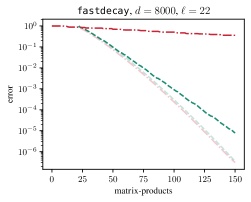
Figure 5: Error as a function of matrix products for CG () and Nyström PCG with $s=1$ () without any reorthgonalization. Light curves show convergence with full-reorthgonalization.

We illustrate this point of comparison explicitly in Figure 5. We run CG and Nyström PCG on the fastdecay problem (for which $\lambda_{1}/\lambda_{d}\gg\lambda_{20}/\lambda_{d}$).

As expected, CG with reorthogonalization burns in for roughly 20 iterations, and then begins converging much more rapidly at a rate depending on $\lambda_{21}/\lambda_{d}$, outperforming Nyström PCG with reorthogonalization ($s=1,\ell=22$), which uses 22 matrix-vector products to build the preconditioner, at which point also converges at a rate depending on $\lambda_{21}/\lambda_{d}$.

However, if reorthogonalization is not used, CG converges at a much slower rate depending on $\lambda_{1}/\lambda_{d}$ while Nyström PCG still converges at the faster rate depending on $\lambda_{21}/\lambda_{d}$.

D.4 What if CG uses some reorthogonalizatoin?

Comparing vanilla CG with Nyström PCG as in Figure 5 is perhaps a bit unfair to CG, since Nyström PCG incurs costs in building, storing, and applying the preconditioner. To put the algorithms on more equal footing, we might allow CG to use a similar amount of storage and arithmetic operations to do some form of reorthogonalization. While there are many complicated schemes based on detailed analyses of the Lanczos algorithm in finite precision arithmetic (Parlet & Scott, 1979; Simon, 1984), a simple scheme is to perform re-orthogonlization only for the first $s\ell$ iterations, and then to continue orthogonalize against these vectors in subsequent iterations. In this case the cost of reorthogonalization during the first $s\ell$ iterations will be $O(ds^{2}\ell^{2})$ operations (the same as the cost to build the the Nyström preconditioner) and subsequently orthogonalizing against these vectors will require $O(ds\ell)$ operations per iteration, the same as the cost to apply the Nyström preconditioner to a vector.

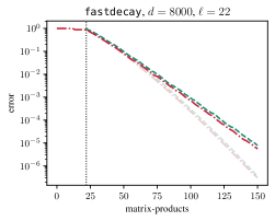
Figure 6: Error as a function of matrix products for CG () with reorthogonalization for $22$ iterations and Nyström PCG with $s=1$ () without any reorthgonalization. Light curves show convergence with full-reorthgonalization.

In Figure 6 we show the behavior of CG with full-reorthogonalization for the first 30 iterations and then orthogonalizing subsequent Krylov basis vectors against these first thirty vectors. Compared to Figure 5, we observe that CG now converges as rapidly as Nyström PCG.

D.5 So what?

A concrete question to address is the following: Under what conditions does CG satisfy a bound like Theorem D.1 in finite precision arithmetic? In particular, does it suffice to orthogonalize the first $O(r)$ vectors to guarantee convergence depending on $\lambda_{r+1}/\lambda_{1}$?

Appendix E More numerical experiments

In this section we provide additional numerical experiments which provide additional insight into the behavior of our augmented block-CG as well as Nyström PCG.

E.1 Convergence

We provide more test problems comparing the convergence of block-CG with Nyström PCG and CG as described in Section 5.1. As observed in Figure 2, block-CG outperforms the other methods in terms of matrix-loads, and often significantly so.

Note that on the outliers20 problem we now append $\ell=22$ Gaussian vectors (rather than $\ell=20$ as shown in Figure 2). This problem has 20 large eigenvalues, and the small amount of oversampling significantly improves the convergence of Nyström PCG with $s=1$.

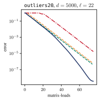
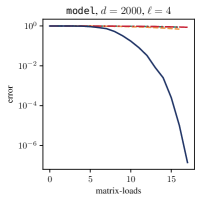
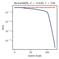
Figure 7: Error versus matrix-loads for block-CG (), CG (), and Nyström PCG with $s=1$ () and $s=3$ () on several test problems; see also Figure 2.

E.2 Impact of finite precision arithmetic

In Section D.3 we discuss why, if no reorthogonalization is used, Nyström PCG may perform better than block-CG or CG. However, as we discuss in Section D.4, a fairer comparison would allow block-CG and CG use some reorthogonalization so that the total number of vectors orthogonalized/stored is equal to the number of vectors used to build the Nyström preconditioner.

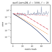
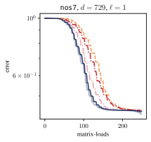
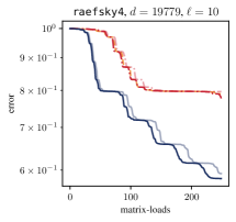
Figure 8: Error versus matrix-loads for block-CG () with reorthogonalization for 3 iterations, CG () with reorthogonalization for $3\ell$ iterations, and Nyström PCG with $s=3$ () without any reorthgonalization. Light curves show convergence of block-CG and CG with no reorthgonalization. The test problems are the same as Figure 2.

In Figure 2 we compare the performance of these methods when we do not use full-reorthogonalzation. In particular, we run Nyström PCG with $s=3$ without any reorthogonalization. Building the preconditioner requires orthogonalizing $s\ell$ vectors. For block-CG and CG use full reorthogonalization until we have a set of $3\ell$ vectors and then continue to orthogonalize only against these vectors. For reference, we also display the convergence of block-CG and CG if no reorthogonalization is used at all.

E.3 Matrix-vector cost

In Figure 9 we show convergence as a function of matrix-vector products on the same test problems as in Figure 2. Here our block-CG underperforms the other methods. This does not conflict with any of our theory, which is in terms of matrix-loads. However, it serves as a reminder that our method may not be suitable in all computational settings; see Section 1.1.

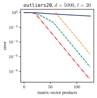
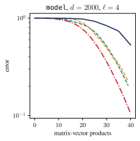
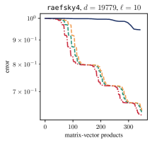
Figure 9: Error versus matrix-products for block-CG (), CG (), and Nyström PCG with $s=1$ () and $s=3$ () on the same test problems as Figure 2.

E.4 Block size

As noted in Section 4.4, we might hope that the accuracy of low-rank approximations to $\mathbf{A}$ built from the information in the block Krylov subspace $\mathcal{K}_{t}(\mathbf{A},\mathbf{\Omega}_{b})$ depends on $bk$, regardless of the individual value of $b$ and $k$. For instance, (Meyer et al., 2024) argues that this is the case for a closely related low-rank approximation algorithm, at least up to logarithmic factors in certain spectral parameters.

In Figure 10, we show the error (after a fixed number of matrix-loads) as a function of the block size, and in Figure 11 we show the condition number of $\mathbf{P}_{\mu}^{-1/2}\mathbf{A}_{\mu}\mathbf{P}_{\mu}^{-1/2}$ as a function of the block size. In some cases Nyström PCG with depth $s=3$ behaves similarly to Nyström PCG with depth $s=1$ when the same number of matrix-vector products are used. For instance, on the outliers20 problem, both methods have a significant drop in the error (due to a significant drop in the condition number) when dimension of the Krylov subspace is roughly equal to $20$, the number of outlying eigenvalues.

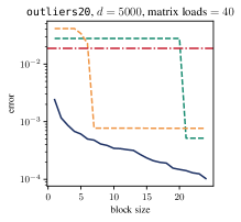
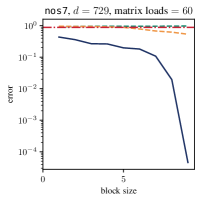
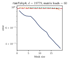
Figure 10: Error versus the Nyström starting block size $\ell$ (number of columns in $\mathbf{\Omega}$) for block-CG (), CG (), and Nyström PCG with $s=1$ () and $s=3$ () on several test problems.

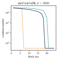
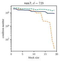
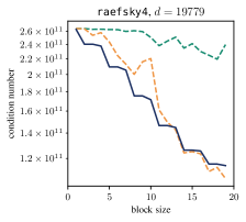
Figure 11: Condition number $\kappa(\mathbf{P}_{\mu}^{-1/2}\mathbf{A}_{\mu}\mathbf{P}_{\mu}^{-1/2})$ of the Nyström preconditioner for $s=1$ () and $s=3$ () as a function of the block size $\ell$ (number of columns in $\mathbf{\Omega}$). For reference, we also show $(\lambda_{\ell+1}+\mu)/(\lambda_{d}+\mu)$ ().

E.5 Test problems

In Figure 12 we show the spectrums of the test problems we used.

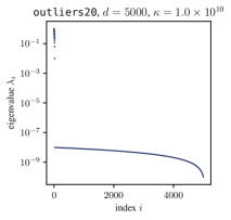
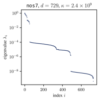
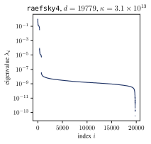
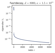
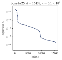
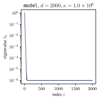
Figure 12: Spectrum of test problems used in this paper.

References

- Bardsley (2012) Bardsley, J. M. Mcmc-based image reconstruction with uncertainty quantification. SIAM Journal on Scientific Computing, 34(3):A1316–A1332, January 2012. ISSN 1095-7197. doi: 10.1137/11085760x.
- Besag et al. (1991) Besag, J., York, J., and Mollié, A. Bayesian image restoration, with two applications in spatial statistics. Annals of the Institute of Statistical Mathematics, 43(1):1–20, March 1991. ISSN 1572-9052. doi: 10.1007/bf00116466.
- Birk & Frommer (2013) Birk, S. and Frommer, A. A deflated conjugate gradient method for multiple right hand sides and multiple shifts. Numerical Algorithms, 67(3):507–529, November 2013. ISSN 1572-9265. doi: 10.1007/s11075-013-9805-9.
- Carson & Daužickaitė (2024) Carson, E. and Daužickaitė, I. Single-pass nyström approximation in mixed precision. SIAM Journal on Matrix Analysis and Applications, 45(3):1361–1391, July 2024. ISSN 1095-7162. doi: 10.1137/22m154079x.
- Chen (2024) Chen, T. The Lanczos algorithm for matrix functions: a handbook for scientists, 2024.
- Chen & Hallman (2023) Chen, T. and Hallman, E. Krylov-aware stochastic trace estimation. SIAM Journal on Matrix Analysis and Applications, 44(3):1218–1244, August 2023. ISSN 1095-7162. doi: 10.1137/22m1494257.
- Chen et al. (2022) Chen, T., Greenbaum, A., Musco, C., and Musco, C. Error bounds for Lanczos-based matrix function approximation. SIAM Journal on Matrix Analysis and Applications, 43(2):787–811, May 2022. ISSN 1095-7162. doi: 10.1137/21m1427784.
- Chow & Saad (2014) Chow, E. and Saad, Y. Preconditioned krylov subspace methods for sampling multivariate gaussian distributions. SIAM Journal on Scientific Computing, 36(2):A588–A608, January 2014. ISSN 1095-7197. doi: 10.1137/130920587.
- Dereziński et al. (2025) Dereziński, M., Musco, C., and Yang, J. Faster linear systems and matrix norm approximation via multi-level sketched preconditioning, January 2025.
- Druskin & Knizhnerman (1991) Druskin, V. L. and Knizhnerman, L. A. Error bounds in the simple Lanczos procedure for computing functions of symmetric matrices and eigenvalues. Comput. Math. Math. Phys., 31(7):20–30, 7 1991. ISSN 0965-5425.
- Díaz et al. (2023) Díaz, M., Epperly, E. N., Frangella, Z., Tropp, J. A., and Webber, R. J. Robust, randomized preconditioning for kernel ridge regression, 2023.
- Epperly et al. (2024) Epperly, E. N., Tropp, J. A., and Webber, R. J. Xtrace: Making the most of every sample in stochastic trace estimation. SIAM Journal on Matrix Analysis and Applications, 45(1):1–23, January 2024. ISSN 1095-7162. doi: 10.1137/23m1548323.
- Feng et al. (1995) Feng, Y., Owen, D., and Perić, D. A block conjugate gradient method applied to linear systems with multiple right-hand sides. Computer Methods in Applied Mechanics and Engineering, 127(1–4):203–215, November 1995. ISSN 0045-7825. doi: 10.1016/0045-7825(95)00832-2.
- Frangella et al. (2023) Frangella, Z., Tropp, J. A., and Udell, M. Randomized nyström preconditioning. SIAM Journal on Matrix Analysis and Applications, 44(2):718–752, May 2023. ISSN 1095-7162. doi: 10.1137/21m1466244.
- Frank & Vuik (2001) Frank, J. and Vuik, C. On the construction of deflation-based preconditioners. SIAM Journal on Scientific Computing, 23(2):442–462, January 2001. ISSN 1095-7197. doi: 10.1137/s1064827500373231.
- Greenbaum (1989) Greenbaum, A. Behavior of slightly perturbed Lanczos and conjugate-gradient recurrences. Linear Algebra and its Applications, 113:7 – 63, 1989. ISSN 0024-3795. doi: 10.1016/0024-3795(89)90285-1.
- Greenbaum (1997) Greenbaum, A. Iterative Methods for Solving Linear Systems. Society for Industrial and Applied Mathematics, Philadelphia, PA, USA, 1997. ISBN 0-89871-396-X.
- Gutknecht (2012) Gutknecht, M. H. Spectral deflation in krylov solvers: a theory of coordinate space based methods. Electron. Trans. Numer. Anal., 39:156–185, 2012.
- Halko et al. (2011) Halko, N., Martinsson, P. G., and Tropp, J. A. Finding structure with randomness: Probabilistic algorithms for constructing approximate matrix decompositions. SIAM Review, 53(2):217–288, January 2011. ISSN 1095-7200. doi: 10.1137/090771806.
- Hestenes & Stiefel (1952) Hestenes, M. R. and Stiefel, E. Methods of conjugate gradients for solving linear systems, volume 49. NBS Washington, DC, 1952.
- Kuss & Rasmussen (2005) Kuss, M. and Rasmussen, C. E. Assessing approximate inference for binary gaussian process classification. Journal of Machine Learning Research, 6(57):1679–1704, 2005.
- Li et al. (2017) Li, H., Linderman, G. C., Szlam, A., Stanton, K. P., Kluger, Y., and Tygert, M. Algorithm 971: An implementation of a randomized algorithm for principal component analysis. ACM Transactions on Mathematical Software, 43(3):1–14, January 2017. ISSN 1557-7295. doi: 10.1145/3004053.
- Martinsson & Tropp (2020) Martinsson, P.-G. and Tropp, J. A. Randomized numerical linear algebra: Foundations and algorithms. Acta Numerica, 29:403–572, May 2020. ISSN 1474-0508. doi: 10.1017/s0962492920000021.
- Meurant (1984) Meurant, G. The block preconditioned conjugate gradient method on vector computers. BIT, 24(4):623–633, December 1984. ISSN 1572-9125. doi: 10.1007/bf01934919.
- Meurant (2006) Meurant, G. The Lanczos and Conjugate Gradient Algorithms. Society for Industrial and Applied Mathematics, 2006. doi: 10.1137/1.9780898718140.
- Meurant & Tichý (2024) Meurant, G. and Tichý, P. Error Norm Estimation in the Conjugate Gradient Algorithm. Society for Industrial and Applied Mathematics, January 2024. ISBN 9781611977868. doi: 10.1137/1.9781611977868.
- Meyer et al. (2024) Meyer, R., Musco, C., and Musco, C. On the Unreasonable Effectiveness of Single Vector Krylov Methods for Low-Rank Approximation, pp. 811–845. Society for Industrial and Applied Mathematics, January 2024. ISBN 9781611977912. doi: 10.1137/1.9781611977912.32.
- Musco & Musco (2015) Musco, C. and Musco, C. Randomized block Krylov methods for stronger and faster approximate singular value decomposition. In Proceedings of the 29th International Conference on Neural Information Processing Systems - Volume 1, volume 28, 2015.
- Musco et al. (2018) Musco, C., Musco, C., and Sidford, A. Stability of the Lanczos method for matrix function approximation. pp. 1605–1624. Society for Industrial and Applied Mathematics, Jan 2018. doi: 10.1137/1.9781611975031.105.
- O’Leary (1980) O’Leary, D. P. The block conjugate gradient algorithm and related methods. Linear Algebra and its Applications, 29:293–322, February 1980. ISSN 0024-3795. doi: 10.1016/0024-3795(80)90247-5.
- Paige (1971) Paige, C. C. The computation of eigenvalues and eigenvectors of very large sparse matrices. PhD thesis, University of London, 1971.
- Paige (1976) Paige, C. C. Error Analysis of the Lanczos Algorithm for Tridiagonalizing a Symmetric Matrix. IMA Journal of Applied Mathematics, 18(3):341–349, 12 1976. ISSN 0272-4960. doi: 10.1093/imamat/18.3.341.
- Parlet & Scott (1979) Parlet, B. N. and Scott, D. S. C. The Lanczos algorithm with selective orthogonalization. Mathematics of Computation, 33(145):217–238, 1 1979. doi: 10.1090/s0025-5718-1979-0514820-3.
- Pleiss et al. (2020) Pleiss, G., Jankowiak, M., Eriksson, D., Damle, A., and Gardner, J. Fast matrix square roots with applications to gaussian processes and bayesian optimization. In Larochelle, H., Ranzato, M., Hadsell, R., Balcan, M., and Lin, H. (eds.), Advances in Neural Information Processing Systems, volume 33, pp. 22268–22281. Curran Associates, Inc., 2020.
- Qiu & Vamanamurthy (1996) Qiu, S.-L. and Vamanamurthy, M. K. Sharp estimates for complete elliptic integrals. SIAM Journal on Mathematical Analysis, 27(3):823–834, May 1996. ISSN 1095-7154. doi: 10.1137/0527044.
- Saad (2003) Saad, Y. Iterative Methods for Sparse Linear Systems. Society for Industrial and Applied Mathematics, January 2003. ISBN 9780898718003. doi: 10.1137/1.9780898718003.
- Simon (1984) Simon, H. D. The lanczos algorithm with partial reorthogonalization. Mathematics of Computation, 42(165):115–142, 1984. ISSN 1088-6842. doi: 10.1090/s0025-5718-1984-0725988-x.
- Thompson (1933) Thompson, W. R. On the likelihood that one unknown probability exceeds another in view of the evidence of two samples. Biometrika, 25(3–4):285–294, December 1933. ISSN 1464-3510. doi: 10.1093/biomet/25.3-4.285.
- Tropp & Webber (2023) Tropp, J. A. and Webber, R. J. Randomized algorithms for low-rank matrix approximation: Design, analysis, and applications, 2023.
- Ubaru et al. (2017) Ubaru, S., Chen, J., and Saad, Y. Fast estimation of via stochastic lanczos quadrature. SIAM Journal on Matrix Analysis and Applications, 38(4):1075–1099, January 2017. ISSN 1095-7162. doi: 10.1137/16m1104974.
- Wang & Jegelka (2017) Wang, Z. and Jegelka, S. Max-value entropy search for efficient bayesian optimization. In Proceedings of the 34th International Conference on Machine Learning - Volume 70, ICML’17, pp. 3627–3635. JMLR.org, 2017.
- Xu & Chen (2024) Xu, Q. and Chen, T. A posteriori error bounds for the block-lanczos method for matrix function approximation. Numerical Algorithms, April 2024. ISSN 1572-9265. doi: 10.1007/s11075-024-01819-7.
- Zhao et al. (2024) Zhao, S., Xu, T., Huang, H., Chow, E., and Xi, Y. An adaptive factorized nyström preconditioner for regularized kernel matrices. SIAM Journal on Scientific Computing, 46(4):A2351–A2376, July 2024. ISSN 1095-7197. doi: 10.1137/23m1565139.
Acknowledgements
We thank Ethan Epperly for useful discussions and feedback.