chebgreen—: Learning and Interpolating Continuous Empirical Green’s Functions from Data

Abstract

In this work, we present a mesh-independent, data-driven library, chebgreen, to mathematically model one-dimensional systems, possessing an associated control parameter, and whose governing partial differential equation is unknown. The proposed method learns an Empirical Green’s Function for the associated, but hidden, boundary value problem, in the form of a Rational Neural Network from which we subsequently construct a bivariate representation in a Chebyshev basis. We uncover the Green’s function, at an unseen control parameter value, by interpolating the left and right singular functions within a suitable library, expressed as points on a manifold of Quasimatrices, while the associated singular values are interpolated with Lagrange polynomials.

1 Introduction

Partial differential Equations (PDEs) have always had a pivotal role in succinctly describing natural phenomena. They allow us to mathematically express the governing fundamental laws, as rate forms [1]. Researchers have worked on data-driven approaches and deep learning techniques to solve PDEs for various systems [2, 3, 4, 5, 6, 7]. Although they hold significant practical importance, the exact PDEs governing many important phenomena remain unknown across fields, including physics, chemistry, biology, and materials science. Thus, there also has been significant work in discovering [8, 9, 10, 11, 12, 13, 14, 15, 16] the underlying PDEs from observational data. Operator Learning represents another significant research avenue; aiming to approximate the solution operator associated with a hidden partial differential equation [17]. Notable contributions in this field include, but are not limited to, Deep Operator Networks [18], Fourier Neural Operators [19], Graph Neural Operator [20], Multipole Graph Neural Operator [21], and Geometry-informed Neural Operator [22]. A detailed overview of the topic can be found in the guide on operator learning [17].

In this paper, our focus is on approximating the Green’s function corresponding to some unknown governing differential equations for a given system of practical interest [23]. There has been recent theoretical work on elucidating learning rates, etc. for Green’s functions learned from data [24, 25, 26], as pertains to systems governed by elliptic or parabolic PDEs. Researchers have also utilized Deep Neural Networks to learn the Green’s function in cases where the underlying operators are weakly non-linear. This approach involves employing a dual auto-encoder architecture to uncover latent spaces where lifting the response data somewhat linearizes the problem, thereby making it more tractable for Green’s function discovery [27]. The field has also advanced through the development of Rational Neural Networks [28], which have been applied to uncover Green’s functions, offering mechanistic insights into the underlying system [29].

The work on learning Empirical Green’s Functions [30] introduces a method for using observational data to learn Green’s functions, in self-adjoint contexts, without relying on machine learning techniques. The approach described in that work proposes learning Empirical Green’s function (EGF) from data in a discrete form,

$$\bm{G} =\bm{U}\bm{\Sigma}\bm{U}^{\top},$$ (1)

$$\bm{G}\in\mathbb{R}^{N_{\text{sensors}}\times N_{\text{sensors}}} \text{, }\bm{U}\in\mathbb{R}^{N_{\text{sensors}}\times K},\bm{\Sigma}\in\mathbb{R}^{K\times K}$$

That same work also proposes a methodology for interpolating these discrete EGF in a principled manner using a manifold interpolation scheme, which derives from the interpolating method for Reduced-order models [31].

In the present work, we utilize the deep learning library, greenlearning, to learn Green’s functions from data [29], and chebfun, the open-source package for computing with functions to high accuracy, in order to improve the work on interpolating Empirical Green’s Functions [30] for 1D linear operators by:

• Extending to non-self adjoint solution operator contexts.

• Reducing the data requirements to learn a Green’s function.

• Introducing a completely mesh-independent formulation for representing the Green’s function.

• Extending the interpolation method to interpolate the continuous representation of the Green’s function.

With greenlearning, we learn the green’s function for a given problem using a synthetic dataset which consists of pairs of forcing functions and the system responses corresponding to those forcing functions. We learn a Neural network, $\mathcal{N}(x,y)$, which approximates the Green’s function $G(x,y)$, $\forall x,y\in\Omega\subset\mathbb{R}$ . We propose creating a low-rank approximation for the neural network, $\mathcal{N}(x,y)$, using our Python implementation of chebfun2 (chebfun in two dimensions [32]), which approximates bivariate functions using Chebyshev polynomials. chebfun2 allows us to construct a Singular Value Expansion (SVE) for the learned Neural network approximating the Green’s function in the form:

$$\mathcal{G}(x,y)=\mathcal{U}_{\infty\times K}\Sigma_{K\times K}\mathcal{V}_{\infty\times K}^{*}$$ (2)

Note that $\mathcal{U}$ and $\mathcal{V}$ are Quasimatrices (a “matrix” in which one of the dimensions is discrete but the other is continuous), and $(\quad)^{*}$ denotes the adjoint of the Quasimatrix. Using this SVE, we interpolate the learned Green’s function using an analogue of our interpolation algorithm from the previous work [30]. This representation, combined with the proposed algorithm, enables interpolation of the Green’s function without discretizing the space, a requirement in previous work [30]. Additionally, it allows storing the Green’s function in a form suitable for high-precision computing [33]. All of this is implemented as a Python package, called chebgreen. Fig. 1 provides a brief overview of the proposed method.

\begin{overpic}[width=433.62pt]{schematic.pdf} \end{overpic}

Figure 1: Schematic of the method for approximating Green’s functions with chebgreen—: First, we approximate the Green’s function from data using greenlearning— [29]; In the second step, our Python— implementation of chebfun— is used to compute a Singular Value Expansion for the learned Green’s function.

In Section 2, we provide a brief introduction to Green’s functions, outline the process of generating our datasets, and present the proposed methods for learning and interpolating Green’s functions. Section 3 features various numerical benchmarks for the method in one dimension, both in the presence and absence of noise. Lastly, concluding remarks are presented in Section 4.

2 Methodology

Consider a linear differential operator, $\mathcal{L}_{\bm{\theta}}$, specified with a set $\bm{\theta}=(\theta_{1},\ldots,\theta_{N_{\text{params}}})\in\mathbb{R}^{N_{\text{params}}}$ of modeling parameters, and defined on a bounded and connected domain $\Omega\subset\mathbb{R}$ in one dimension, assumed to govern a physical system in the form of a boundary value problem:

$$\mathcal{L}_{\bm{\theta}}u =f, \text{on }\Omega,$$ (3)

$$\mathcal{B}u =g, \text{in }\partial\Omega,$$

where, $\mathcal{B}$ is a linear differential operator specifying the boundary conditions of the problem ($g$ being the constraint on the problem boundary, $\partial\Omega$), $f$ is a forcing (or source) term, and $u$ is the unknown system response. It is pointed out that, while only a single boundary condition is shown in Eq. 3, in an actual problem setting there would be a sufficient number of such conditions to ensure well-posedness. Under suitable conditions on the operator, there exists a Green’s function $G_{\bm{\theta}}:\Omega\times\Omega\to\mathbb{R}$ associated with $\mathcal{L}_{\bm{\theta}}$ that is the impulse response of the linear differential operator and defined [23] as:

$$\mathcal{L}_{\bm{\theta}}G_{\bm{\theta}}(x,s)=\delta(s-x),\quad x,s\in\Omega,$$

where, $\mathcal{L}$ acts on the first variable and $\delta$ is the Dirac delta function. Then with homogeneous Dirichlet boundary conditions, i.e., $\mathcal{B}u=0$ on the boundary of the domain, the solution to Eq. 3, for a forcing, $f$, can be expressed using the Green’s function within a Fredholm integral equation of the first-kind:

$$\tilde{u}(x)=\int_{\Omega}G_{\bm{\theta}}(x,s)f(s)ds,\qquad x,s\in\Omega.$$

Now, if we consider the homogeneous solution to Eq. 3, $u_{\text{hom}}$, which can be found by solving the following boundary value problem:

$$\mathcal{L}_{\bm{\theta}}u_{\text{hom}} =0,$$

$$\mathcal{B}u =g.$$

we can use superposition, to construct solutions, $u$, to Eq. 3 as $u=\tilde{u}+u_{\text{hom}}$,

$$u(x)=\int_{\Omega}G_{\bm{\theta}}(x,s)f(s)ds+u_{\text{hom}},\qquad x,s\in\Omega$$ (4)

In this work, we only consider examples where $\bm{\theta}=\theta\in\mathbb{R}$, or $N_{\text{param}}=1$, but all the proofs and methods can be trivially extended to work for $N_{\text{param}}\geq 2$. We begin with a description of the data (in our case synthetic data generated from simulations) which we use to learn the Green’s functions.

2.1 Generating the dataset

The datasets used to learn Green’s functions consist of $N_{\text{samples}}\geq 1$ forcing terms, $\{f_{j}\}_{j=1}^{N_{\text{samples}}}$, and the corresponding system’s responses, $\{u_{j}\}_{j=1}^{N_{\text{samples}}}$, satisfying Eq. 3. In the present work, our systems (3) are forced with random functions, sampled from a Gaussian process (GP), $\mathcal{GP}(0,K)$, with a covariance kernel, $K$, as motivated by recent theoretical results [24]. More specifically, the forcing terms are drawn from a GP, with mean zero and squared-exponential covariance kernel, $K_{\text{SE}}$, defined as:

$$K_{\text{SE}}(x,s)=\exp\left(-\dfrac{|x-s|^{2}}{2l^{2}}\right),\quad x,s\in\Omega,$$

where, $\Omega=[a,b]\subset\mathbb{R}$ is the one-dimensional problem domain and $l>0$ is the length scale hyperparameter that sets the correlation length for this kernel. Similar to greenlearning [29], we define a normalized length scale parameter, $\sigma=l/(b-a)$, in order to remove the dependence on the length of the domain. This parameter, $\sigma$ is chosen to be larger than the spatial discretization at which we are numerically evaluating the forcing terms; to ensure that the random functions are resolved properly within the discrete representation employed. Additionally, $\sigma$ is specified to possess a suitable magnitude in order to ensure that the set of forcing terms is of full numerical rank. Note that other types of covariance kernels used in recent deep learning studies [34], such as Green’s functions related to Helmholtz equations, are likely to produce improved approximation results, as they inherently contain some information about the singular vectors of the operator, $\mathcal{L}_{\theta}$. This is reflected in the theoretical bounds for the randomized SVD with arbitrary covariance kernels, which show that one may obtain higher accuracy by incorporating knowledge of the leading singular vectors of the differential operator into the covariance kernel [25]. In the present work, we employ a generic squared-exponential kernel as one may not have prior information about the governing operator, $\mathcal{L}_{\theta}$, in real applications. In the case of problems with a periodic boundary conditions we draw the forcing functions from the periodic kernel:

$$K_{\text{Periodic}}(x,s)=\exp\left(-\dfrac{2\sin^{2}(\pi|x-s|/p)}{l^{2}}\right),\quad x,s\in\Omega,$$

where $p$ is the desired period of the functions.

We are interested in applications where one can only measure the responses at a finite number of locations, $\bm{x}=\{x_{1},\ldots,x_{N_{x}}\}$, where ${x}_{i}\in\Omega$ and $N_{x}\geq 1$ is the number of measurements taken within the domain, $\Omega$. Similarly, we sample the forcing terms at $\bm{s}=\{s_{1},\ldots,s_{N_{s}}\}$, where ${s}_{i}\in\Omega$ and $N_{s}\geq 1$ to assemble the following column vectors:

$$f_{i}=f_{i}(\bm{s})\coloneqq\begin{bmatrix}f_{i}(s_{1})&\cdots&f_{i}(s_{N_{s}})\end{bmatrix}^{\top},\quad u_{i}=u_{i}(\bm{x};\theta)\coloneqq\begin{bmatrix}u_{i}(x_{1})&\cdots&u_{i}(x_{N_{x}})\end{bmatrix}^{\top},$$

The notation $u_{i}(\bm{x};\theta)$ highlights the dependence of the responses on the parameter $\theta$, and $\top$ denotes the matrix transpose. We collect these as $N_{\text{samples}}$ number of input-output pairs as $\{f_{i},u_{i}\}$. In order to gauge fidelity of the learned Green’s function to the true underlying Green’s function, during training, we leave out a part of our dataset ($\sim 5\%$) to serve as a validation dataset and don’t use this during our learning process.

$$\{f_{i},u_{i}\}_{i=1}^{N_{\text{samples}}}=\{f_{i},u_{i}\}_{i=1}^{N_{\text{train}}}+\{f_{i},u_{i}\}_{i=1}^{N_{\text{validation}}}$$

2.2 Low-rank approximation of the Green’s function

We want to compute a low-rank approximation for the Green’s function $G_{\theta}$ associated with the linear differential operator, $\mathcal{L}_{\theta}$, by employing a singular value expansion (SVE) :

$$\mathcal{G}_{\theta}(x,y)=\sum_{k=1}^{K}\sigma_{k}\phi_{k}(y)\psi_{k}(x),$$ (5)

where, $\sigma_{1}\geq\dots\geq\sigma_{K}\geq 0$ are the singular values, $\{\phi_{k}\}_{k=1}^{K}$ are the left singular functions, and $\{\psi_{k}\}_{k=1}^{K}$ are the right singular functions. Here, each term $\sigma_{k}\psi_{k}(y)\psi_{k}(x)$ is a rank 1 approximation which can be thought of as an “outer product” of two univariate functions.

2.3 Approximating Green’s functions with Neural Networks

In order to compute an efficient approximation for the Green’s function, $\mathcal{G}_{\theta}(x,y)$, we use the method developed by Boullé et al. [29]. The main idea is to train two Rational Neural Networks [28]: $\mathcal{N}_{\text{G}}(x,s)$ which approximates the Green’s function associated with the underlying linear differential, $\mathcal{L}_{\theta}$; and $\mathcal{N}_{\text{hom}}(x)$ which corresponds to the homogeneous solution associated with the boundary conditions, by minimizing the following loss over our training dataset $\{f_{i},u_{i}\}_{i=1}^{N_{\text{train}}}$:

$$\text{Loss}=\frac{1}{N_{\text{train}}}\sum_{i=1}^{N_{\text{train}}}\frac{1}{\|u_{i}\|_{L^{2}(\Omega)}^{2}}\int_{\Omega}\left(u_{i}(x)-\mathcal{N}_{\text{hom}}(x)-\int_{\Omega}\mathcal{N}_{\text{G}}(x,s)f_{i}(s)ds\right)^{2}dx$$ (6)

We propose a slight modification to the loss function for problems where we know that the boundary conditions are Dirichlet. In these case, the Green’s function is zero on the boundaries. More explicitly, if the problem is defined on the domain $\Omega=[a,b]\subset\mathbb{R}$, and the boundary conditions are Dirichlet,

$$G_{\theta}(a,s)=G_{\theta}(b,s)=G_{\theta}(x,a)=G_{\theta}(x,b)=0,\quad x,s\in\Omega.$$

Incorporating this information in the loss function improves the fidelity of the computed left and right singular functions (described in Section 2.5) near the boundaries of the domain. We utilize Approximate Distance Functions [35] to enforce this by changing the loss function slightly to

$$\text{Loss}=\frac{1}{N_{\text{train}}}\sum_{i=1}^{N_{\text{train}}}\frac{1}{\|u_{i}\|_{L^{2}(\Omega)}^{2}}\int_{\Omega}\left(u_{i}(x)-\mathcal{N}_{\text{hom}}(x)-\int_{\Omega}\alpha(x,s)\mathcal{N}_{\text{G}}(x,s)f_{i}(s)ds\right)^{2}dx,$$ (7)

where, $\alpha(x,s)$ is the Approximate Distance Function for a rectangular domain. To construct this, we start from the approximate distance function for a line segment [36] that joins $\bm{x}_{1}\equiv(x_{1},s_{1})$ and $\bm{x}_{2}\equiv(x_{2},s_{2})$, with a center $\bm{x}_{c}\equiv(\bm{x}_{1}+\bm{x}_{2})/2$ and length $L=\|\bm{x}_{1}-\bm{x}_{2}\|$:

$$\beta\equiv\beta(\bm{x})=\sqrt{h^{2}+\left(\dfrac{\varphi-t}{2}\right)^{2}},\quad\varphi=\sqrt{t^{2}+h^{4}},$$

where,

$$h\equiv h(\bm{x}) =\dfrac{(x-x_{1})(s_{2}-s_{1})-(s-s_{1})(x_{2}-x_{1})}{L},$$

$$t\equiv t(\bm{x}) =\dfrac{1}{L}\left[\left(\dfrac{L}{2}\right)^{2}-\|\bm{x}-\bm{x}_{c}\|^{2}\right].$$

\begin{overpic}[width=303.53267pt]{adf.pdf} \end{overpic}

Figure 2: Example of the approximate distance function for a domain $[-4,2]\times[-4,2]$.

We then combine the approximate distance functions for the four segments, $\{\beta_{1},\beta_{2},\beta_{3},\beta_{4}\}$ with an R-equivalence solution that preserves normalization up to order $m=1$ of the distance function at all regular points, given by [37]:

$$\alpha(x,s)=\beta(\beta_{1},\beta_{2},\beta_{3},\beta_{4})=\dfrac{1}{\sqrt[m]{\dfrac{1}{\beta_{1}^{m}}+\dfrac{1}{\beta_{2}^{m}}+\dfrac{1}{\beta_{3}^{m}}+\dfrac{1}{\beta_{4}^{m}}}}$$

An example of the approximate distance function is shown in Fig. 2. In the cases where the problem does not have a Dirichlet boundary condition or the boundary conditions are unknown, we set $\alpha(x,s)\equiv 1$.

To compute the loss function described in (7), the integrals are discretized using a trapezoidal rule [38] over the measurement locations for the forcing terms $\{s_{i}\}_{i=1}^{N_{s}}$ and the system responses $\{x_{i}\}_{i=1}^{N_{x}}$. This gives us a bivariate function as a product of Rational Neural Network with a fixed function (which is defined purely in terms of the domain boundaries), $g(x,s)=\alpha(x,s)\mathcal{N}_{\text{G}}(x,s)$, which approximates the Green’s function associated with our problem. Now we would like to construct a singular value expansion (SVE) for this bivariate function. To do so, we implemented the necessary parts of the chebfun MATLAB library [33] in Python as chebpy2, using the 1D implementation, chebpy [39]. In the next two subsections, we describe the basic details of how chebfun constructs a SVE for bivariate functions using polynomial interpolants in a Chebyshev basis.

2.4 Approximating a bivariate function, $g(x,y)$, with chebfun2

A chebfun is a polynomial interpolant of a smooth function $f:[-1,1]\to\mathbb{R}$ evaluated at $n+1$ Chebyshev points, and furnished with:

$$x_{i}=\cos\left(\frac{i\pi}{N}\right),\quad 0\leq i\leq N$$

After adaptively choosing a polynomial degree, $N$, to approximate $f$ to machine precision, a chebfun stores these $N+1$ values $(f(x_{i}))_{0\leq i\leq N}$ as a vector, whose entries are the coefficients for a Lagrange basis,

$$f(x)\approx\sum_{i=0}^{N}f(x_{i})l_{i}(x),\quad l_{i}(x)=\frac{\prod_{j=0,j\neq i}^{N}(x-x_{j})}{\prod_{j=0,j\neq i}^{N}(x_{i}-x_{j})}$$

Approximating a function with a chebfun allows for constructing infinite-dimensional analogues of matrices, which are called Quasimatrices. A column Quasimatrix can be thought of as $\infty\times K$ matrices. In other words, they have finitely many columns, each column being represented by a square-integrable function, in this case a chebfun.

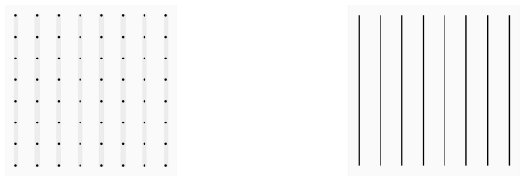
Figure 3: Entries in the column, represented by dots, of a matrix (left) can be replaced by a chebfun—, represented by a solid line, in a Quasimatrix (right)

Consider a $\infty\times K$ column Quasimatrix $\mathcal{A}$, where $\{\mathcal{A}_{k}\}_{k=1}^{K}$ are chebfun-s on some domain $\Omega\subset\mathbb{R}$.

$$\mathcal{A}:=\left[\begin{array}[]{ccc}\mathcal{A}_{1}&\dots&\mathcal{A}_{K}\end{array}\right]$$ (8)

We may also view this Quasimatrix $\mathcal{A}$ as an element of the vector space $(L^{2}(\Omega))^{K}$. This is a natural space to look for low-rank approximations to a Hilbert-Schmidt integral operator such as those associated with certain Green’s functions, as they are compact operators on the Hilbert space $L^{2}(\Omega)$. We start by defining a few operations on the Quasimatrix. For some scalar $c$,

$$c\mathcal{A}=\mathcal{A}c:=\left[\begin{array}[]{ccc}c\mathcal{A}_{1}&\dots&c\mathcal{A}_{K}\end{array}\right]$$

For a $K\times K$ matrix $C$, we can define its product with a Quasimatrix as:

$$\mathcal{A}C:=\left[\begin{array}[]{ccccc}\sum_{j=1}^{K}C_{j1}\mathcal{A}_{j}&\dots&\sum_{j=1}^{K}C_{jk}\mathcal{A}_{j}&\dots&\sum_{j=1}^{K}C_{jK}\mathcal{A}_{j}\end{array}\right]$$

Similarly, for a row Quasimatrix $\mathcal{B}:=\left[\begin{array}[]{ccc}\mathcal{B}_{1}&\dots&\mathcal{B}_{K}\end{array}\right]^{\top}$, which can be thought of as a $K\times\infty$ matrix, such that each row is a chebfun, one can define:

$$C\mathcal{B}:=\left[\begin{array}[]{c}\sum_{j=1}^{K}\mathcal{B}_{j}C_{1j}\\ \vdots\\ \sum_{j=1}^{K}\mathcal{B}_{j}C_{kj}\\ \dots\\ \sum_{j=1}^{K}\mathcal{B}_{j}C_{Kj}\end{array}\right]$$

In this paper, we will denote the adjoint of a column Quasimatrix $\mathcal{A}$ as $\mathcal{A}^{*}$, and note that, given another column Quasimatrix $\mathcal{C}$, the inner product between two quasimatrices (an outer product on the space $(L^{2}(\Omega))^{K}$) is given by [40]:

$$\mathcal{A}^{*}\mathcal{C}:=\left[\begin{array}[]{ccc}\left(\mathcal{A}_{1},\mathcal{C}_{1}\right)_{L^{2}(\Omega)}&\cdots&\left(\mathcal{A}_{1},\mathcal{C}_{K}\right)_{L^{2}(\Omega)}\\ \vdots&\ddots&\vdots\\ \left(\mathcal{A}_{K},\mathcal{C}_{1}\right)_{L^{2}(\Omega)}&\cdots&\left(\mathcal{A}_{K},\mathcal{C}_{K}\right)_{L^{2}(\Omega)}\end{array}\right]\in\mathbb{R}^{K\times K}$$ (9)

Although we are not considering the case of Quasimatrices with complex-valued functions as columns, we use the notation $\mathcal{A}^{*}$ rather than $\mathcal{A}^{\top}$ in order to distinguish from the usual matrix transpose, as both of these operations show up in the proofs in the Appendix.

The idea of employing a polynomial approximation of a univariate function on a Chebyshev grid can be extended to approximate bivariate functions. chebfun2 [32] constructs approximate $g(x,y)\approx C(y)DR(x)$. It constructs a rank $K$ approximant as follows:

$$g(x,y)\approx g_{k}(x,y)=\sum_{k=1}^{K}D_{k}C_{k}(y)R_{k}(x)$$ (10)

Here, each $C_{k},R_{k}$ is a chebfun and $D_{k}\in\mathbb{R}$ is a pivot value. The $Chebfun$-s $C_{k}$ are collected into one quasimatrix $C(y)=[C_{1}(y),C_{2}(y),\dots,C_{K}(y)]$, and $R_{k}$ into another quasimatrix $R(x)=[R_{1}(x),R_{2}(x),\dots,R_{K}(x)]$.

While constructing the approximation, chebfun2 chooses pivot, $(x_{k},y_{k})$ on the domain of the bivariate function and constructs a column chebfun $C_{k}(y)$ to approximate $G(x_{k},y)$ and a row chebfun $R_{k}(x)$ to approximate $G(x,y_{k})$.

Figure 4: Example of pivot locations on a grid

The pivots are chosen at the locations where the absolute error between the current approximant and the bivariate function $G(x,y)$ is maximum. Repeating this procedure iteratively for $K$ steps, chebfun2 constructs an approximation for $g(x,y)$. A more detailed overview of the workings of chebfun2 can be found in the original work [32].

2.5 Constructing a singular value expansion of $g(x,y)$

Note that the end-goal of using chebfun2 is to construct a singular value expansion for $G(x,y)$ as follow:

$$g(x,y)=\mathcal{U}_{\infty\times K}(y)\Sigma_{K\times K}\mathcal{V}_{\infty\times K}^{*}(x)$$

Constructing this Singular Value Expansion thus requires computing a QR decomposition of a Quasimatrix. The details of the same can be found in Trefethen’s work on Householder triangularization of a Quasimatrix [41]. The main details are summarized here.

Let’s assume we want to find a QR decomposition for a $\infty\times n$ Quasimatrix $\bm{A}$, the columns of which are functions of $x\in[a,b]$ ($\bm{A}$ is a linear map from $\mathbb{C}^{n}$ to $L^{2}[a,b]$). Let the notation $\bm{v}^{*}\bm{w}$ denote the inner product and $\|\cdot\|$ be the $L^{2}$ norm on $[a,b]$. We would like to decompose this Quasimatrix as $\bm{A}=\bm{Q}\bm{R}$, such that $\bm{Q}$ is an orthonormal Quasimatrix and $\bm{R}$ is an upper triangular matrix. The aim is to compute this by the numerically more stable method of Householder reflections. This is done by applying a self-adjoint operator, $\bm{H}$, so that one can get the form as shown in Fig. 5. Here, the vertical lines denote that the column is a chebfun.

Figure 5: Householder triangularization of a Quasimatrix

$\bm{E}$ will be an $\infty\times n$ quasimatrix , fixed in advanced, with orthonormal columns $\{e_{j}\}$, and $\bm{S}$ is an $n\times n$ sign matrix, so as to ensure the diagonal of $\bm{R}$ is real and non-negative. In practice, $e_{j}$ is taken to be a multiple of the $(j-1)$th Legendre polynomial $P_{j-1}(x)$, scaled to $[a,b]$. The Householder reflector $\bm{H}_{k}$ is a self-adjoint operator acting on $L^{2}[a,b]$, chosen so as to map a certain function to another function of equal norm in the space spanned by $e_{1},\dots,e_{k}$.

The precise formulas to compute these components corresponding for each column $k\in 1,\dots,n$ are as follows:

$$\bm{x}=\bm{A}[:,k],\quad\bm{R}_{kk}=\|\bm{x}\|,\quad\bm{S}_{k}=-\text{sign}(e^{*}_{k}\bm{x}),$$

$$\bm{y}=\bm{S}_{k}\bm{R}_{kk}e_{k},\quad\bm{v}=\frac{\bm{y}-\bm{x}}{\|\bm{y}-\bm{x}\|},\quad\bm{H}_{k}=\bm{I}-2\bm{v}\bm{v}^{*},$$

$$\bm{A}[:,j]=\bm{H}_{k}\bm{A}[:,j],\quad\bm{R}_{kj}=e^{*}_{k}\bm{A}[:,j],\quad\bm{A}[:,j]=\bm{A}[:,j]-\bm{R}_{kj}e_{k},\quad k+1\leq j\leq n.$$

Here, the outer product notation $\bm{v}\bm{v}^{*}$ denotes the operator that maps a function $\bm{w}$ to $\bm{v}(\bm{v}^{*}\bm{w})$. Since $\bm{H}_{1}\cdots\bm{H}_{n}$ is the adjoint of $\bm{H}$ in $L^{2}[a,b]$, $\bm{Q}=\bm{H}_{1}\cdots\bm{H}_{n}\bm{E}\bm{S}$. This gives us our QR decomposition.

The process of constructing an SVE with chebfun2 [32] is outlined in Algorithm 1.

Algorithm 1 SVE using chebfun2—

Input: A chebfun $G(x,y)\approx C(y)DR(x)$

Output: Quasimatrices with orthonormal columns $\mathcal{U}_{G}$ and $\mathcal{V}_{G}$, and a diagonal matrix $\Sigma_{G}$

1. Householder triangularization: $C(y)=Q_{C}(y)R_{C}$, $R(x)^{*}=Q_{R}(x)R_{R}$.

2. Compute: $A=R_{C}DR_{R}^{*}$.

3. Matrix SVD: $A=U_{A}S_{A}V_{A}^{*}$.

4. Compute: $\mathcal{U}_{G}=Q_{C}(y)U_{A}$, $\mathcal{V}_{G}=Q_{R}(x)V_{A}$, and $\Sigma_{G}=S_{A}$.

This gives us the singular value expansion we desire:

$$g(x,y)\approx\mathcal{U}_{g}(y)\Sigma_{g}\mathcal{V}^{*}_{g}(x)$$

2.6 chebgreen—: Combining greenlearning— and chebfun—

With these two key components, we can efficiently learn and store a singular value expansion for a Green’s function, starting from data in the form of input (forcing functions) - output (system responses) pairs, for the “unknown” underlying linear differential equation:

• Learn two Rational Neural networks, $\mathcal{N}_{\text{G}}(x,s)$ and $\mathcal{N}_{\text{hom}}(x)$, from the training data, $\{f_{i},u_{i}\}_{i=1}^{N_{\text{train}}}$ to approximate the Green’s functions as $g(x,y)=\alpha(x,s)\mathcal{N}_{G}(x,s)$ along with the homogeneous solution, $u_{\text{hom}}=\mathcal{N}_{\text{hom}}(x)$.

• Use our Python implementation of the chebfun library to represent these approximations in a Chebyshev basis:

  • We store the Green’s function as a singular value expansion of a chebfun2:

    $$g(x,s;\theta) =\alpha(x,s)\mathcal{N}_{G}(x,s;\theta),$$

    $$\mathcal{G}_{\theta}(x,s) \equiv\mathcal{U}(y;\theta)\Sigma(\theta)\mathcal{V}^{*}(x;\theta)=\mathcal{U}_{g}(y)\Sigma_{g}\mathcal{V}^{*}_{g}(x)=g(x,s;\theta).$$

  • The homogeneous solution is stored as a chebfun:

    $$\mathcal{H}(x)\equiv\mathcal{N}_{\text{hom}}(x).$$

2.7 Interpolating the solution on a manifold

The algorithm proposed by Praveen et al.[30] relies on the method of interpolating in a tangent space of the compact Stiefel manifold. The compact $k-$Stiefel manifold of $\mathbb{R}^{m}$ is defined to be the manifold of equivalence classes of $m\times k$ matrices with orthonormal columns, where $U$ and $U^{\prime}$ are consiedered equivalent when their columns span the same subspace of $\mathbb{R}^{m}$ [42]. In other words, we may think of it as

$$S_{k}(\mathbb{R}^{m})=\{{U\in\mathbb{R}^{m\times k}\colon U^{T}U=I_{k}}\}.$$ (11)

Their previous algorithm takes the SVDs of known Green’s functions, $G_{i}=\Phi_{i}\Sigma_{i}\Phi_{i}^{T}$, at parameters $\theta_{i}$, chooses an index $j$ that is closest to the unseen parameter, $\theta^{*},$ and lets $\Phi_{j}=\hat{\Phi}$ be the reference basis (base point) for the interpolation. The other known orthonormal matrices, $\Phi_{i}$, represented as elements on the Stiefel manifold, are then mapped to the tangent space at $\hat{\Phi}$ via an approximation to the logarithmic map [43]. These points in the tangent space are then interpolated via Lagrange polynomial interpolation, and the matrix, $\Phi^{*}$, for the unseen parameter, $\theta^{*}$, is obtained by mapping the interpolated point back to the Stiefel manifold from the tangent space using an exponential mapping [43].

We wish to generalize this method to the case where the orthonormal matrices $\Phi$ are instead rank $k$ operators represented by a quasimatrix whose $k$ columns are $L^{2}(\Omega)$ functions, where $\Omega$ is a suitable domain. In other words, whereas in the finite dimensional problem we were interested in $m\times k$ real matrices, here we are interested in the space $H=(L^{2}(\Omega))^{k},$ which may also be thought of as $\mathcal{L}(\mathbb{R}^{k},L^{2}(\Omega)),$ the space of linear transformations from $\mathbb{R}^{k}$ to $L^{2}(\Omega).$

In order to generalize the manifold interpolation, we first need to find a space analogous to the finite-dimensional Stiefel manifold, and to identify its tangent space [40]. We write elements, $\Phi$, of $H$ in row-vector notation as $\Phi=(\Phi_{1},...,\Phi_{k}),$ so that we can multiply quasimatrices (viewed here as vectors in $H$) on the right by a $k\times k$ matrix to get another vector in $H.$ The space $H$ admits an outer product [40]

$$\Phi^{*}\Psi:=\left[\begin{array}[]{ccc}\left(\Phi_{1},\Psi_{1}\right)_{L^{2}(\Omega)}&\cdots&\left(\Phi_{1},\Psi_{k}\right)_{L^{2}(\Omega)}\\ \vdots&\ddots&\vdots\\ \left(\Phi_{k},\Psi_{1}\right)_{L^{2}(\Omega)}&\cdots&\left(\Phi_{k},\Psi_{k}\right)_{L^{2}(\Omega)}\end{array}\right]\in\mathbb{R}^{k\times k}$$ (12)

as well as an inner product

$$(\Phi,\Psi)_{H}:=\sum_{j=1}^{k}\left(\Phi_{j},\Psi_{j}\right)_{L^{2}(\Omega)}=\operatorname{tr}(\Phi^{*}\Psi).$$ (13)

Here, we use the suggestive notation $\Phi^{*}\Psi$ for the outer product on $H$ to emphasize that this is both distinct from, and analogous with, the matrix transpose [44]. We then define

$$S_{K}(H)=\{{\Phi\in H\colon\Phi^{*}\Phi=I_{K}}\}.$$ (14)

The inner product on $H$ induces a Riemannian metric, and turns $S_{k}(H)$ into a Riemannian submanifold of $H$ which we will call the Stiefel manifold, and will denote from here on simply by $S_{k}$ [40]. It can be shown that its tangent space at a point $\Phi$ is

$$T_{\Phi}S_{K}=\{{\Psi\in H\colon\Psi^{*}\Phi=-\Phi^{*}\Psi\}}$$ (15)

which is analogous to the identification of the tangent space for the finite dimensional Stiefel manifold.

The next step towards extending the manifold interpolation algorithm to the Quasimatrix case is to find an orthogonal projection mapping from $H$ to $T_{\Phi}S_{k},$ the tangent space of the Stiefel manifold at $\Phi.$ We established the following result, which we will prove in the appendix of this paper:

Theorem 1.

The map $P_{\Phi}\colon H\rightarrow T_{\Phi}S_{K}$ given by $\Psi\mapsto\Psi-\Phi\operatorname{sym}(\Phi^{*}\Psi)$, where $\operatorname{sym}(\Phi^{*}\Psi)\coloneq\frac{1}{2}(\Phi^{*}\Psi+\Psi^{*}\Phi)$, is the orthogonal projection onto the tangent space of the Stiefel manifold $S_{K}$ at $\Phi.$

This projection mapping is our infinite dimensional analogue to Step 4 Part 1 of the previous algorithm [30].

In order to extend the third part of Step 4 of that same algorithm to the Quasimatrix generalization, we need to establish a valid approximation to the exponential map so that we can map interpolated points in the tangent space back to the Stiefel manifold. The key concept is that of a retraction on a manifold, which may be thought of as a first order approximation to the exponential map. In their previous algorithm Praveen et al.[30] use QR factorization as their approximation to the exponential map, as it is retraction on the finite dimensional Stiefel manifold. Altman et al. [40] show that Quasimatrix QR factorization is a retraction on our infinite dimensional Stiefel manifold $S_{k}$, so it follows that we may simply use the Quasimatrix version of QR factorization as our approximation to the exponential map in our updated algorithm.

Algorithm 2 Interpolation of continuous EGFs to unseen modeled parameters

Input: A set of singular functions and values, $\{[\mathcal{U}(s;\theta_{j}),\Sigma(\theta_{j}),\mathcal{V}(x;\theta_{j}),\theta_{j}]\}_{j=1}^{N_{\text{models}}}$ to be interpolated for a new parameter instance, $\theta_{*}$.

Step 1: From among the $\theta_{j}$’s, identify a $\theta_{0}$, as being closest to $\theta_{*}$, and use the associated left singular functions, $\mathcal{U}(s;\theta_{0})$, as the reference basis for the interpolation. Similarly, $\mathcal{V}(x;\theta_{0})$ is the reference basis for interpolating the right singular functions.

Step 2: Correct sign flips and shuffling of both left and right singular functions according to the left singular functions, $\mathcal{U}(s;\theta_{0}))$.

Step 3: Perform the interpolation:

1. Lift the left and right singular functions to the tangent spaces $\mathcal{T}_{\mathcal{U}_{0}}S_{K}$ and $\mathcal{T}_{\mathcal{V}_{0}}S_{K}$ respectively, by using the following map,

   $$\Gamma^{\mathcal{U}_{0}}_{j} =\mathcal{U}(s;\theta_{j}))-\mathcal{U}(s;\theta_{0}))\ \text{sym}\left(\mathcal{U}^{*}(s;\theta_{0}))\mathcal{U}(s;\theta_{j}))\right),$$

   $$\Gamma^{\mathcal{V}_{0}}_{j} =\mathcal{V}(x;\theta_{j}))-\mathcal{V}(x;\theta_{0}))\ \text{sym}\left(\mathcal{V}^{*}(x;\theta_{0}))\mathcal{V}(x;\theta_{j}))\right),\quad\text{sym}\left(Y\right)\coloneqq(Y+Y^{*})/2.$$

2. Using Lagrange polynomials, compute the interpolated tangent quasimatrices, $\Gamma^{\mathcal{U}}_{*}$ and $\Gamma^{\mathcal{V}}_{*}$, using $\{[\Gamma^{\mathcal{U}}_{j},\Gamma^{\mathcal{U}}_{j}]\}_{j=1}^{N_{models}}$. Interpolate the coefficients, $\{\tilde{\Sigma}(\theta_{j})\}_{j=1}^{N_{models}}$, with the same scheme, to obtain $\Sigma(\theta_{*})$.

3. Compute the interpolated left and right singular functions, $\mathcal{U}(s;\theta_{*}),\mathcal{V}(x;\theta_{*})$, by mapping $\bm{\Gamma}_{*}$ back to $\mathcal{S}_{K}$ using the exponential map,

   $$\mathcal{U}(s;\theta_{*})=\text{qf}(\mathcal{U}(s;\theta_{0})+\Gamma^{\mathcal{U}}_{*}),$$

   $$\mathcal{V}(x;\theta_{*})=\text{qf}(\mathcal{V}(x;\theta_{0})+\Gamma^{\mathcal{V}}_{*}),$$

   where $\text{qf}(A)$ denotes the $Q$ factor of the QR decomposition of $A\in\mathbb{R}^{\infty\times r}$.

Step 4: Order the singular functions and values to match the left singular functions at the initial parameter instance, $\theta_{0}$.

Output: Interpolated left singular functions, $\mathcal{U}(s;\theta_{*})$, right singular functions, $\mathcal{V}(x;\theta_{*})$ and singular values $\Sigma(\theta_{*})$ at parameter $\theta_{*}$.

Fig. 6 depicts a schematic of the described interpolation method from Algorithm 2.

\begin{overpic}[width=325.215pt]{interpolation.pdf} \end{overpic}

Figure 6: The points on the “Stiefel” manifold (represented by the orthonormal quasimatrices $\mathcal{U}_{j}$) are projected onto the flat tangent space $\smash{\mathcal{T}_{\mathcal{U}_{0}}S_{K}}$ at the reference basis $\smash{\mathcal{U}_{0}=\mathcal{U}(s;\theta_{0})}$, where they are interpolated and then returned to the compact Stiefel manifold as $\mathcal{U}_{*}$.

2.7.1 Correcting eigenmodes sign and order

The approximation for the Green’s function, $\mathcal{G}_{\theta}(x,s)\equiv\mathcal{U}(y;\theta)\Sigma(\theta)\mathcal{V}^{*}(x;\theta)$, constructed in Section 2.6, is stored as a singular value expansion within a library of other such expansions, one each for the collection of model parameters, $\theta$, considered. As singular value expansion orders the singular functions according to the magnitude of the singular values by construction, the singular functions may swap their order as the parameter $\theta$ varies. If we consider the one-dimensional Helmholtz equation with frequency $\theta\geq 0$ and homogeneous boundary conditions:

$$\frac{d^{2}u}{dx^{2}}+\theta^{2}u=f,\quad x\in[0,1],\quad\text{or}\quad\mathcal{L}_{\theta}=\frac{d^{2}}{dx^{2}}+\theta^{2}.$$

We observe that the first two singular functions swap at some critical value of $\theta$. The $k^{\text{th}}$ singular value for the Green’s functions of the operator $\mathcal{L}_{\theta}$ are given by $\sigma_{k}=1/(\theta^{2}-(k\pi)^{2})$. If we compare the first two modes, they satisfy $|\sigma_{1}|>|\sigma_{2}|$, when $\theta<\sqrt{5/2}\pi$, and $|\sigma_{1}|\leq|\sigma_{2}|$ otherwise. This implies that the first two eigenmodes are swapped when $\theta>\sqrt{5/2}\pi$, as illustrated by Fig. 7, and that the manifold interpolation technique will perform poorly in such cases. The same phenomena occurs for the higher eigenmodes at larger values of $\theta$. We propose to reorder the singular functions and the associated singular values of the discovered basis at the given interpolation parameter to match the ones at the origin point $\theta_{0}$, where we lift to the tangent space of the infinite-dimensional analogue for Stiefel manifold. For a given parameter, $\theta_{j}$, and mode number, $1\leq k\leq K$, we select the $k^{\text{th}}$ left singular function at $\theta_{j}$ to be the one with minimal angle with the $k^{\text{th}}$ left singular function at parameter $\theta_{0}$, i.e.,

$$\mathcal{U}_{k}(y;\theta_{j})=\mathcal{U}_{\ell^{\prime}}(y;\theta_{j}),\quad\text{where}\quad\ell^{\prime}=\text{match}(k),$$

$$\text{match}(k)= \operatorname*{arg\,max}_{1\leq\ell\leq K,\ell\neq\text{match}(k^{\prime})\forall 1\leq k^{\prime}<k}|\langle\mathcal{U}_{\ell}(y;\theta_{j}),\mathcal{U}_{k}(y;\theta_{0})\rangle|,\quad 1\leq k\leq K.$$

where $\langle\cdot,\cdot\rangle$ denotes the inner product in the continuous $L^{2}$ sense. Note that the reordering is done by matching the left singular functions, starting from the left singular function with the highest singular value, without replacement. When the order of the left singular functions has been changed by this procedure, we also re-order the corresponding singular values and right singular functions to preserve the value of the Green’s function.

\begin{overpic}[width=433.62pt]{mode_swap.pdf} \end{overpic}

Figure 7: (A) Magnitude of the first two eigenvalues of the Green’s function associated with the one-dimensional Helmholtz equation. The first two corresponding eigenmodes are swapped when the frequency, $\theta$, increases beyond the critical value of $\theta_{\text{crit}}=\sqrt{5/2}\pi\approx 5$, as displayed in (B) and (C).

Another potential issue arises because singular functions are unique only up to a sign flip. Thus, learning approximations to Green’s functions at two different parameters close to each other, $\theta_{1}$ and $\theta_{2}$ say, might lead to singular functions associated with the $k^{\text{th}}$ singular value being very “dissimilar” between the Green’s functions learned at the respective parameter value, $\theta$. In order to best align the singular functions before interpolation, we account for these sign flip by comparing the the left and right singular functions of the learned approximations with an inner product. Consider the left singular functions at the origin of the manifold, $\mathcal{U}_{k}(s;\theta_{0}))$ (implying the $k^{\text{th}}$ left singular function), around which we form the tangent space. We compute an inner product between the left singular functions of the other interpolants, $\mathcal{U}_{k}(s;\theta_{j}))$, and the corresponding left singular functions at the origin, $\mathcal{U}_{k}(s;\theta_{0})$, in order to correct the signs for the left and right singular functions of the interpolant, as follows:

$$\mathcal{U}_{k}(s;\theta_{j}),\mathcal{V}_{k}(x;\theta_{j})\equiv\begin{cases}-\mathcal{U}_{k}(s;\theta_{j}),-\mathcal{V}_{k}(x;\theta_{j})&\text{if}\ \langle\mathcal{U}_{k}(s;\theta_{j}),\mathcal{U}_{k}(s;\theta_{0})\rangle<0,\\ \mathcal{U}_{k}(s;\theta_{j}),\mathcal{V}_{k}(x;\theta_{j})&\text{otherwise}.\end{cases}$$

Note that the reshuffling of the singular functions is performed before correcting for the sign flips as we are making the assumption that the singular functions associated with the $k^{\text{th}}$ singular value across models are somewhat correlated.

3 Numerical results

In this section, we exemplify the use of our methods on a number of synthetic problems. Unless specified otherwise, the hyperparameters involved in generating the dataset, learning and storing the Green’s function, and interpolating the same are as follows:

• Generating the dataset: The length scale of the squared exponential covariance kernel in the Gaussian Process from which the forcing terms are sampled is set to $\sigma=10^{-2}$. The forcing terms and system responses are measured on a uniform 1D grid at $N_{\text{x}}=N_{\text{s}}=500$ equally spaced points. It is crucial that the density of sampling points is chosen so that functions are sufficiently resolved on the grid, i.e., and the discrete vector of values at the sampling locations are free from spatial aliasing. In our case, since the forcing terms and responses are sampled from a continuous representation in a Chebyshev basis (using chebfun), we use the number of Chebyshev points used to represent these functions as a proxy for the number of samples needed on a uniform grid. Note that equispaced points suffer from Runge Phenomenon [45] so a uniform grid is not optimal for representing these functions but data are generally collected at uniform grids in experiments; thus we chose to test our methods in a such a setting. Finally, the number of input-output pairs is set to $N_{\text{samples}}=250$, out of which only $~95\%$ are used during training.

• Greenlearning: Each of the neural network used to learn the Green’s function and the homogeneous solution are $4$-layer Rational Neural Networks having $50$ neurons within each layer. They are trained for $2000$ epochs using the Adam optimizer with a learning rate of $10^{-2}$, and the learning rate decaying exponentially to $10^{-3}$ over the $2000$ epochs.

• chebpy2: When learning polynomial approximations for one and two-dimensional functions using chebpy2, we specify the accuracy of the functions that need to be resolved in the domain as $\varepsilon^{\text{cheb}}\approx 2.22\times 10^{-16}$. In case of two dimensions, we specify this value for each of the independent variable within the domain, $\varepsilon^{\text{cheb}}_{x}$ and $\varepsilon^{\text{cheb}}_{s}$ for $G(x,s)$. These are both set to $\varepsilon^{\text{cheb}}_{x}=\varepsilon^{\text{cheb}}_{s}\approx 2.22\times 10^{-16}$. We choose the value of $\approx 2.22\times 10^{-16}$, which is the eps - the difference between $1.0$ and the next smallest representable floating point number larger than $1.0$ for single floating point precision, in a direction for all experiments as our neural networks are trained with float64 (double floating point) precision. In the cases where there is noise in the collected data, as is the case when data are collected from experiments, this number can be set close to the noise floor so that the model does not overfit to noise. However, in our numerical experiments with noise, we do not change this number, so as to demonstrate the robustness of our method to noise.

For doing experiments with noisy dataset, we artificially pollute the system responses, $u_{i}$, with additive, white Gaussian noise as:

$$u^{\text{noisy}}_{i}(x_{j})=u_{i}(x_{j})+\zeta c_{i,j}\overline{|u_{i}|},\quad 1\leq i\leq N_{\text{sensors}},$$

where $\overline{|u_{i}|}$ is the average of the absolute value of the $i$th system’s response and the $c_{i,j}\sim\mathcal{N}(0,1)$ are independent and identically distributed. The noise level is controlled by the parameter $\zeta$ which we have set to $\zeta=0.5$, which corresponds to $50\%$ noise in the output.

In the cases, where we know the analytical Green’s function for our numerical experiments, we can assess the learned Green’s function in an $L^{2}$-sense, we define the “relative error” as:

$$\epsilon=\dfrac{\|\mathcal{G}(x,s)-G_{\text{exact}}(x,s)\|_{L^{2}(\Omega\times\Omega)}}{\|G_{\text{exact}}(x,s)\|_{L^{2}(\Omega\times\Omega)}}$$ (16)

where, $\mathcal{G}(x,s)$ is the chebgreen model of the Green’s function and $G_{\text{exact}}(x,s)$ is the closed-form Green’s function of the underlying operator. However, this is not possible in all cases since the closed-form for the Green’s function is not known in all cases. In these cases, we propose that one can compute a “test error” by reconstructing the system responses for unseen data (the $5\%$ of the dataset we leave out for validation during training). For this paper, we generate a testing dataset with $N_{\text{test}}=100$ pairs of forcing functions and system responses, $\{f_{i},u_{i}\}_{i=1}^{N_{\text{test}}}$ and compute the test error as:

$$\epsilon_{\text{test}}=\dfrac{1}{N_{\text{test}}}\sum_{i=1}^{N_{\text{test}}}\dfrac{\|\tilde{u}_{i}-u_{i}\|_{L^{2}(\Omega)}}{\|u_{i}\|_{L^{2}(\Omega)}}\times 100\%,\quad\tilde{u}_{i}=\int_{\Omega}\mathcal{G}(x,s)f_{i}(s)ds+\mathcal{H}(x).$$ (17)

In the next part of this section, we limit discussion to cases where the homogeneous solution, $\mathcal{H}(x)$, lives within a sub-space to the given problem’s solution space (e.g. homogeneous Dirichlet and periodic cases).

3.1 Poisson problem

Before we demonstrate our method’s efficacy for interpolation, we will approximate the Green’s function, and it’s singular value expansion, for a one-dimensional Laplacian operator. Assume we have a Poisson problem with homogeneous boundary conditions defined as follows:

$$-\frac{d^{2}}{dx^{2}}u(x)=f(x),\quad x\in[0,1],\quad u(0)=u(1)=0.$$ (18)

For this is a canonical problem, the closed-form solution for the associated Green’s function is known and is given by:

$$G_{\text{exact}}=\begin{cases}x(1-s),\quad\text{if }x\leq s,\\ s(1-x),\quad\text{if }x>x,\end{cases}$$

where $x,s\in[0,1]$.

Using chebgreen, we learn the Green’s function for the underlying Laplacian operator using noise-free data, as shown in Fig. 8. On visual inspection, the Green’s function learned by chebgreen (Fig. 8A) matches closely with the analytical Green’s function for Eq. 18 (Fig. 8B). In Fig. 8C, we plot the relative error between the learned and analytical Green’s function,

$$\epsilon_{G}=\dfrac{|\mathcal{G}(x,s)-G_{\text{analytical}}(x,s)|}{\|G_{\text{analytical}}(x,s)\|_{L^{2}([0,1]\times[0,1])}}$$

as an error contour. The relative error $\epsilon=0.36\%$ indicates satisfactory the fidelity of our learned Green’s function to the analytical solution. Finally, we observe that the first five learned left (Fig. 8D) and right (Fig. 8F) singular functions are indistinguishable from the left and right singular functions of the analytical solution of the Green’s function. In Fig. 8E, we plot the first 100 learned singular values for the Green’s function against the analytical values of the singular values, $1/(\pi^{2}k^{2})$. There is an exponential decay for the smallest singular values in case of the learned Green’s function. We use Rational NN to approximate the Green’s function which is a smooth approximation to the exact Green’s function; thus, this fast decay is expected. The key point is that the largest learned singular values are in close agreement with analytical solution. Therefore, our method constructs a high-fidelity low-rank approximation of the Green’s function associated with Laplacian operator.

\begin{overpic}[width=433.62pt]{images/laplace.pdf} \end{overpic}

Figure 8: (A) Approximation of the Green’s functions learned by chebgreen—, (B) Analytical solution of the Green’s function associated with the Laplacian operator, (C) Relative error contour between the learned model and analytical solution, (D) First 5 Left Singular Functions of the learned Green’s function, (E) Comparison of the learned singular values against the analytical singular values for the Green’s function, and (F) First 5 Right Singular Functions of the learned Green’s function.

Fig. 9A shows how the relative error for the learned Green’s function, $\epsilon$, changes as a function of the noise level, $\zeta$, for the system responses in the training dataset. Note that we only consider the effect of output noise in this case. An instance of a possible sample from the dataset with $\zeta=0.6$ ($60\%$ noise) is shown in Fig. 9: B is the forcing function used to perturb the system, and C is the corresponding clean system response (blue) along with the artificially polluted system response (red). Finally, the error contour of the Green’s function learned with a dataset with noise level $\zeta=0.6$ against the analytical Green’s function is shown in Fig. 9D. The relative error is $\epsilon=1.38\%$. Thus, even when the system responses barely resemble the underlying function (because of noise), our method seems to works well; learning a reasonably accurate approximation to the underlying Green’s function.

\begin{overpic}[width=433.62pt]{images/laplace_noise_study.pdf} \end{overpic}

Figure 9: (A) Relative error at different noise level, $\zeta$, for the Laplacian operator, (B) Instance of a forcing function, (C) Instance of a system response with and without white Gaussian noise at level $\zeta=0.6$ ($60\%$ noise), and (D) Contours for relative error between the learned model with a noisy dataset at $\zeta=0.6$ and analytical solution for the Laplacian operator.

3.2 Advection-Diffusion

As the next problem, we learn and interpolate the Green’s function associated with the operator in a parameterized Advection-Diffusion case, described by the following boundary value problem:

$$\frac{d^{2}}{dx^{2}}u(x)+\theta\frac{d}{dx} u(x)=f(x),\quad x\in[-1,1],$$

$$u(-1)=u(1)=0.$$

Thus, the operator for which we would like to find a Green’s functions (in the domain $x\in[-1,1]$) is:

$$\mathcal{L}_{\theta}=\frac{d^{2}}{dx^{2}}+\theta\frac{d}{dx}$$

\begin{overpic}[width=433.62pt]{images/advection_diffusion.pdf} \end{overpic}

Figure 10: (A-C) Approximation of the Green’s functions associated with the Advection-Diffusion problem at $\theta=1,2,3$ used by the interpolation scheme. (D) Interpolated Green’s function at $\theta_{*}=2.5$. (E) The target Green’s function approximated by chebgreen—.

We learn approximations to the Green’s functions for the associated non self-adjoint linear operator at the parameter values $\theta_{1}=1.0$, $\theta_{2}=2.0$, and $\theta_{3}=3.0$. The test error for the approximations is less than $0.29\%$; computed using our small training set with $N_{\text{train}}=237$ input-output pairs for each $\theta$.

Using these three interpolants, we compute an interpolated model at $\theta_{*}=2.5$. We also compute a target model (ground truth), or a model compute with data generated at $\theta_{*}=2.5$ for comparison. As we can see in Fig. 10, the interpolated and the target Green’s functions are in close agreement, on visual inspection. The test error for the interpolated Green’s function at $\theta_{*}$ is equal to $\epsilon_{\text{test}}=0.54\%$. In this case, we can also compare the interpolated Green’s function against the analytical solution by computing the relative error, which is $\epsilon=0.26\%$. This demonstrates that our model can approximate Green’s functions for non self-adjoint linear operators extremely well with a small amount of data as well as the manifold interpolation technique provides a great framework to interpolate these learned models based on some parameter value.

3.3 Airy Problem

After establishing the fidelity of the Green’s function learned and interpolated by our method to the analytical expression for the same in cases where these were available, we now demonstrate chebgreen on problems where the analytical form of the Green’s function is not known. To this end, we parameterize the Airy equation in the following way:

$$\frac{d^{2}u}{dx^{2}}-\theta^{2}xu=f,\quad x\in[0,1],$$

In this case, we demonstrate both interpolation and extrapolation capabilities of chebgreen:

3.3.1 Interpolation

For the interpolation case, we compute the three approximations to the Green’s functions for the parameterized operator at $\theta_{1}=1.0$, $\theta_{2}=5.0$, and $\theta_{3}=10.0$ (we call these the ”interpolant” cases). The left and right singular functions for this problem vary significantly as we change the value of $\theta$ as seen in Fig. 11, which makes it a useful test for our interpolation method.

\begin{overpic}[width=433.62pt]{images/airy_modes.pdf} \end{overpic}

Figure 11: (A) First and (B) Second learned Left Singular Function for the airy problem at $\theta_{1}=1.0$, $\theta_{2}=5.0$, and $\theta_{3}=10.0$

Note that since the values of the parameter $\theta$ are much further apart compared to the Advection-Diffusion case, and $\theta$ appear as a squared quantities in the operator, we expect the differences in the learned Green’s function to be much more drastic. This is evident from the learned Green’s function shown in Fig. 12A-C. The interpolated Green’s function at $\theta_{*}$ has a test error of $\epsilon_{\text{test}}=2.76\%$. This is larger than the test errors for the interpolant cases (less than $0.69\%$). Although given we are interpolating using only three points on an non-linear manifold, our method seems to perform reasonably well.

\begin{overpic}[width=433.62pt]{images/airy_interpolation.pdf} \end{overpic}

Figure 12: (A-C) Approximation of the Green’s functions associated with the Airy problem at $\theta=1,5,10$ used by the interpolation scheme. (D) Interpolated Green’s function at $\theta_{*}=7$. (E) The target Green’s function approximated by chebgreen—.

3.3.2 Extrapolation

In order to demonstrate the ability of our method to generalize out of the neighborhood of the approximated Green’s functions, we compute chebgreen approximations at $\theta_{1}=6.0$, $\theta_{2}=7.0$, and $\theta_{3}=8.0$ and extrapolate to $\theta_{*}=9.0$. This satisfactory performance is due to our having learned a suitable solution operator (i.e., Green’s function). A visual comparison between the extrapolated model and a target model constructed with data at $\theta_{*}=9.0$ is shown in Fig. 13.

\begin{overpic}[width=346.89731pt]{images/airy_extrapolation.pdf} \end{overpic}

Figure 13: (A) Extrapolated Green’s function. (B) The target Green’s function approximated by chebgreen— at $\theta_{*}=9$.

3.4 Fractional Laplacian

As a final example, we consider a non-local operator in the form of a one-dimensional fractional Laplacian having periodic boundary conditions:

$$(-\Delta)^{\theta}u=f,\quad u\left(-\dfrac{\pi}{2}\right)=u\left(-\dfrac{\pi}{2}\right),\quad x\in\left[-\dfrac{\pi}{2},\dfrac{\pi}{2}\right]$$ (19)

where $0<\theta<1$ is the fractional order. To generate the dataset for this problem, we use a Fourier spectral collocation to solve Eq. 19. The forcing and system responses are sampled at a slightly smaller uniform 1D grid, with $N_{x}=N_{s}=600$ samples. For chebfun, we set $\varepsilon_{x}^{\text{cheb}}=\varepsilon_{s}^{\text{cheb}}=1\times 10^{-9}$ as the Green’s function tends to be non-differentiable throughout the domain which makes it difficult to resolve this to float64 precision.

We follow the same procedure of approximating three Green’s functions at parameter values $\theta_{1}=0.8$, $\theta_{2}=0.9$, and $\theta_{3}=0.95$ and interpolating to $\theta_{*}=0.9$. The test error for the interpolated model is equal to $\epsilon_{\text{test}}=0.99\%$ which is comparable to the test error for the interpolant cases (less than $0.95\%$). A visual comparison of the interpolated model against the target model is shown in Fig. 14C-D.

\begin{overpic}[width=433.62pt]{images/fractional_laplacian.pdf} \end{overpic}

Figure 14: (A-C) Approximation of the Green’s functions associated with the Fractional Laplacian problem at $\theta=0.8,0.9,0.95$ used by the interpolation scheme. (D) Interpolated Green’s function at $\theta_{*}=0.85$. (E) The target Green’s function approximated by chebgreen—.

3.5 Summary of errors for all problems

The test errors for all the interpolant, interpolated, and target Green’s functions are summarized in Table 1. We also compute the test errors when the dataset has $50\%$ output noise (noise level $\zeta=0.5$). Note that here we learn the Green’s function with the noisy dataset but we test with a clean dataset; to demonstrate that we indeed learn the underlying solution operator. The test error on the noisy dataset for these cases are available in Table 2.

Problem	$\theta_{1}$	$\theta_{2}$	$\theta_{3}$	Interpolated	Target
Airy	0.38 (1.87)	0.69 (1.91)	0.62 (2.02)	2.76 (3.28)	0.76 (1.84)
Fractional Laplacian	0.51 (2.38)	0.95 (2.81)	0.65 (1.87)	0.99 (2.94)	0.41 (2.21)
Advection Diffusion	0.24 (1.57)	0.26 (1.49)	0.29 (1.49)	0.54 (1.61)	0.3 (1.54)

Table 1: Summary of the test error for the Airy, Fractional Laplacian, and Advection-Diffusion problems. The error for experiments with noisy dataset are shown in parenthesis.

4 Conclusions

In this work, we propose an extension of the previous work [30] on learning and interpolating Green’s function from data. Some notable improvements include the inclusion of greenlearning [29] to learn an approximation of Green’s function in form of a continuous, bivariate function and the use of our python implementation of chebfun library [33], chebpy, to learn a Singular Value Expansion instead of Singular Value Decomposition, in the previous work [30]. This allows the new method to learn a representation which is not tied to a particular discretization of the domain, making it truly mesh-independent. Finally, the novel generalization of the previous interpolation algorithm for orthonormal matrices on Stiefel manifold to the interpolation of Quasimatrices on the infinite dimensional analogue of Stiefel manifold, provides a way to seamlessly use the machinery we have created in order learn the solution operator for 1D parametric linear partial differential equations. We present multiple examples in order to demonstrate that the method learns high-fidelity approximations to the underlying Green’s function of a linear operator with an order of magnitude lower data requirement compared to the previous work. We also demonstrate that the proposed method is robust against large amounts of noise in the dataset. This, along with the easy to use library which is available online makes it a useful tool for use in discovering the solution operators in realistic experimental settings.

Data availability

The code used to produce the numerical results is publicly available on GitHub at https://github.com/hsharsh/chebgreen for reproducibility purposes.

Appendix A Proof for interpolating quasimatrices on tangent space of $H=(L^{2}(\Omega))^{K}$ space

Theorem 1.

The map $P_{\Phi}\colon H\rightarrow T_{\Phi}S_{K}(H)$ given by $\Psi\mapsto\Psi-\Phi\operatorname{sym}(\Phi^{*}\Psi)$ is the orthogonal projection onto the tangent space of the Stiefel manifold $S_{K}(H)$ at $\Phi,$ where $\operatorname{sym}(\Phi^{*}\Psi)\coloneq\frac{1}{2}(\Phi^{*}\Psi+\Psi^{*}\Phi).$

Proof.

Let $A=\Phi^{*}\Psi$ and $B=\Psi^{*}\Phi.$ First we show that $P_{\Phi}$ is a projection operator, i.e. that $P_{\Phi}\circ P_{\Phi}=P_{\Phi}.$ For $\Psi\in H,$ we have

$$P_{\Phi}(P_{\Phi}(\Psi))=\Psi-\frac{1}{2}\Phi(A+B)-\frac{1}{2}\Phi\left([\Psi-\frac{1}{2}\Phi(A+B)]^{*}\Phi+\Phi^{*}[\Psi-\frac{1}{2}\Phi(A+B)]\right)$$

$$=\Psi-\frac{1}{2}\Phi(A+B)-\frac{1}{2}\Phi\left(\Psi^{*}\Phi-[\frac{1}{2}\Phi(A+B)]^{*}\Phi+\Phi^{*}\Psi-\Phi^{*}[\frac{1}{2}\Phi(A+B)]\right)$$

$$=\Psi-\frac{1}{2}\Phi(A+B)-\frac{1}{2}\Phi\left(A-\frac{(A+B)}{2}\Phi^{*}\Phi+B-\Phi^{*}\Phi\frac{(A+B)}{2}\right)$$

Since $\Phi$ is an element of the Stiefel manifold, it satisfies $\Phi^{*}\Phi=I_{K}.$ So all of the terms in the last line to the right of $\Psi-\frac{1}{2}\Phi(A+B)$ cancel out, and it follows that $P_{\Phi}P_{\Phi}=P_{\Phi}$ as desired.

Next, we must show that $P_{\Phi}$ is self-adjoint in order to establish that it is an orthogonal projection. For any $\Psi,\Gamma\in H,$ we have

$$\operatorname{tr}\left(P_{\Phi}(\Psi)^{*}\Gamma\right)=\operatorname{tr}\left(\Psi^{*}\Gamma-\frac{1}{2}\left[\Phi(\Phi^{*}\Psi+\Psi^{*}\Phi)\right]^{*}\Gamma\right),$$

and

$$\operatorname{tr}\left(\Psi^{*}P_{\Phi}(\Gamma)\right)=\operatorname{tr}\left(\Psi^{*}\Gamma-\frac{1}{2}\Psi^{*}\left[\Phi(\Phi^{*}\Gamma+\Gamma^{*}\Phi)\right]\right).$$

So it suffices to show that

$$\operatorname{tr}\left(\left[\Phi(\Phi^{*}\Psi+\Psi^{*}\Phi)\right]^{*}\Gamma\right)=\operatorname{tr}\left(\Psi^{*}\left[\Phi(\Phi^{*}\Gamma+\Gamma^{*}\Phi)\right]\right).$$ (20)

To see that left side of Eq. (A.1) satisfies

$$\operatorname{tr}\left(\left[\Phi(\Phi^{*}\Psi+\Psi^{*}\Phi)\right]^{*}\Gamma\right)=\operatorname{tr}\left((\Phi^{*}\Psi+\Psi^{*}\Phi)(\Phi^{*}\Gamma)\right)$$ (21)

consider the left side of Eq. (A.2),

$$\operatorname{tr}\left([\Phi(\Phi^{*}\Psi+\Psi^{*}\Phi)]^{*}\Gamma\right)=\operatorname{tr}\left([\Phi(\Phi^{*}\Psi)]^{*}\Gamma+[\Phi(\Psi^{*}\Phi)]^{*}\Gamma\right),$$

note that computing the term in the left of trace argument, $[\Phi(\Phi^{*}\Psi)]^{*}\Gamma,$ gives a $k\times k$ matrix $C$ such that

$$C_{ij}=\left(\sum_{i=1}^{k}\Phi_{i}(\Phi_{j},\Psi_{k})_{L^{2}(\Omega)},\Gamma_{j}\right)_{L^{2}(\Omega)}.$$

Expanding right side of Eq. (A.2),

$$\operatorname{tr}\left((\Phi^{*}\Psi+\Psi^{*}\Phi)(\Phi^{*}\Gamma)\right)=\operatorname{tr}\left((\Phi^{*}\Psi)(\Phi^{*}\Gamma)+(\Psi^{*}\Phi)(\Phi^{*}\Gamma)\right)$$

and multiplying out the term $(\Phi^{*}\Psi)(\Phi^{*}\Gamma)$, we find that this is equal to $C=[\Phi(\Phi^{*}\Psi)]^{*}\Gamma.$ Doing the same computation for the other term, we conclude that Eq. (A.2) holds.

Similarly, the right side of Eq. (A.1) gives

$$\operatorname{tr}\left(\Psi^{*}\left[\Phi(\Phi^{*}\Gamma+\Gamma^{*}\Phi)\right]\right)=\operatorname{tr}\left((\Psi^{*}\Phi)(\Phi^{*}\Gamma+\Gamma^{*}\Phi)\right)$$

Using the fact that $(\Xi^{*}\Omega)^{T}=\Omega^{*}\Xi$ for any $\Xi,\Omega\in H,$ which comes from the definition of the outer product on $H$ in Eq. (8), it follows that Eq. (A.1) holds. Hence $P_{\Phi}$ is an orthogonal projection.

Finally, to see that the image of $P_{\Phi}$ is all of $T_{\Phi}S_{K}(V),$ consider the operator $P^{\perp}_{\Phi}$ defined by the mapping $\Psi\mapsto\Phi\operatorname{sym}(\Phi^{*}\Psi).$ The normal space may be characterized as the set of all elements of $H$ of the form $\Phi M$ where $M$ is a symmetric matrix. Clearly any element of the normal space is the image of some $\Psi$ under this mapping. Since we have $\Psi=P_{\Phi}(\Psi)+P^{\perp}_{\Phi}(\Psi)$ for any $\Psi\in H,$ it follows that $P_{\Phi}$ is the orthogonal projection onto $T_{\Phi}S_{K}(H).$ ∎

Appendix B Test error for interpolation cases with noisy dataset

Problem	$\theta_{1}$	$\theta_{2}$	$\theta_{3}$	Interpolated	Target
Airy	6.74	6.76	6.83	7.46	6.78
Fractional Laplacian	7.52	7.55	7.48	7.58	7.49
Advection Diffusion	6.63	6.61	6.69	6.65	6.66

Table 2: Summary of the empirical error for the Airy, Fractional Laplacian, and Advection-Diffusion problems, in the case where the models are learned and tested on a noisy dataset.

References

- [1] R. P. Feynman, The Character of Physical Laws, M.I.T. Press, 1967.
- [2] M. Raissi, Deep hidden physics models: Deep learning of nonlinear partial differential equations, J. Mach. Learn. Res. 19 (1) (2018) 932–955.
- [3] M. Raissi, G. E. Karniadakis, Hidden physics models: Machine learning of nonlinear partial differential equations, J. Comput. Phys. 357 (2018) 125–141.
- [4] J. Berg, K. Nyström, Neural network augmented inverse problems for PDEs, arXiv preprint arXiv:1712.09685 (2017).
- [5] L. Lu, X. Meng, Z. Mao, G. E. Karniadakis, Deepxde: A deep learning library for solving differential equations, SIAM Review 63 (2021) 208–228.
- [6] J. Sirignano, K. Spiliopoulos, Dgm: A deep learning algorithm for solving partial differential equations, Journal of Computational Physics 375 (2018) 1339–1364. doi:10.1016/J.JCP.2018.08.029.
- [7] E. Weinan, B. Yu, The deep ritz method: A deep learning-based numerical algorithm for solving variational problems, Communications in Mathematics and Statistics 6 (2018) 1–12.
- [8] M. Raissi, P. Perdikaris, G. E. Karniadakis, Physics-informed neural networks: A deep learning framework for solving forward and inverse problems involving nonlinear partial differential equations, J. Comput. Phys. 378 (2019) 686–707.
- [9] H. Schaeffer, Learning partial differential equations via data discovery and sparse optimization, Proc. R. Soc. A 473 (2197) (2017) 20160446.
- [10] S. L. Brunton, J. L. Proctor, J. N. Kutz, Discovering governing equations from data by sparse identification of nonlinear dynamical systems, Proc. Natl. Acad. Sci. U.S.A. 113 (15) (2016) 3932–3937.
- [11] K. Champion, B. Lusch, J. N. Kutz, S. L. Brunton, Data-driven discovery of coordinates and governing equations, Proceedings of the National Academy of Sciences of the United States of America 116 (2019) 22445–22451.
- [12] S. H. Rudy, S. L. Brunton, J. L. Proctor, J. N. Kutz, Data-driven discovery of partial differential equations, Sci. Adv. 3 (4) (2017) e1602614.
- [13] C. Bonneville, C. Earls, Bayesian deep learning for partial differential equation parameter discovery with sparse and noisy data, J. Comput. Phys.: X 16 (2022) 100115.
- [14] R. Stephany, C. Earls, PDE-READ: Human-readable partial differential equation discovery using deep learning, Neural Netw. 154 (2022) 360–382.
- [15] R. Stephany, C. Earls, Pde-learn: Using deep learning to discover partial differential equations from noisy, limited data, Neural Networks 174 (2024) 106242.
- [16] R. Stephany, C. Earls, Weak-pde-learn: A weak form based approach to discovering pdes from noisy, limited data, Journal of Computational Physics 506 (6 2024).
- [17] N. Boullé, A. Townsend, A mathematical guide to operator learning, Handbook of Numerical Analysis 25 (2024) 83–125. doi:10.1016/BS.HNA.2024.05.003.
- [18] L. Lu, P. Jin, G. Pang, Z. Zhang, G. E. Karniadakis, Learning nonlinear operators via deeponet based on the universal approximation theorem of operators, Nature Machine Intelligence 3 (2021) 218–229.
- [19] Z. Li, N. Kovachki, K. Azizzadenesheli, B. Liu, K. Bhattacharya, A. Stuart, A. Anandkumar, Fourier neural operator for parametric partial differential equations, Advances in Neural Information Processing Systems 33 (2020) 6755–6766.
- [20] Z. Li, N. Kovachki, K. Azizzadenesheli, B. Liu, K. Bhattacharya, A. Stuart, A. Anandkumar, Neural operator: Graph kernel network for partial differential equations, arXiv preprint arXiv:2003.03485 (3 2020).
- [21] Z. Li, N. Kovachki, K. Azizzadenesheli, B. Liu, K. Bhattacharya, A. Stuart, A. Anandkumar, Multipole graph neural operator for parametric partial differential equations, Proceedings of the 34th International Conference on Neural Information Processing Systems (2020).
- [22] Z. Li, N. Kovachki, C. Choy, Boyi, J. Kossaifi, S. P. Otta, M. A. Nabian, M. Stadler, C. Hundt, , K. Azizzadenesheli, A. Stuart, A. Anandkumar, Geometry-informed neural operator for large-scale 3d pdes, Proceedings of the 37th International Conference on Neural Information Processing Systems (2023) 35836 – 35854.
- [23] L. Evans, Partial differential equations, 2nd Edition, American Mathematical Society, 2010.
- [24] N. Boullé, A. Townsend, Learning elliptic partial differential equations with randomized linear algebra, Found. Comput. Math. (2022) 1–31.
- [25] N. Boulle, A. Townsend, A generalization of the randomized singular value decomposition, in: International Conference on Learning Representations, 2022.
- [26] N. Boullé, S. Kim, T. Shi, A. Townsend, Learning green’s functions associated with time-dependent partial differential equations, The Journal of Machine Learning Research 23 (2022) 1–34. doi:10.5555/3586589.3586807.
- [27] C. R. Gin, D. E. Shea, S. L. Brunton, J. N. Kutz, DeepGreen: Deep learning of Green’s functions for nonlinear boundary value problems, Sci. Rep. 11 (1) (2021) 1–14.
- [28] N. Boulle, Y. Nakatsukasa, A. Townsend, Rational neural networks, Advances in Neural Information Processing Systems 33 (2020) 14243–14253.
- [29] N. Boullé, C. J. Earls, A. Townsend, Data-driven discovery of Green’s functions with human-understandable deep learning, Sci. Rep 12 (1) (2022) 1–9.
- [30] H. Praveen, N. Boullé, C. Earls, Principled interpolation of green’s functions learned from data, Computer Methods in Applied Mechanics and Engineering 409 (2023) 115971. doi:10.1016/J.CMA.2023.115971.
-
[31]
D. Amsallem, C. Farhat, Interpolation method for adapting reduced-order models and application to aeroelasticity, AIAA Journal 46 (2008) 1803–1813.
doi:10.2514/1.35374.
URL https://arc.aiaa.org/doi/abs/10.2514/1.35374 - [32] A. Townsend, L. N. Trefethen, An extension of chebfun to two dimensions, SIAM Journal on Scientific Computing 35 (12 2013). doi:10.1137/130908002.
- [33] T. A. Driscoll, N. Hale, L. N. Trefethen, Chebfun Guide, Pafnuty Publications, 2014.
- [34] Z. Li, N. B. Kovachki, K. Azizzadenesheli, B. liu, K. Bhattacharya, A. Stuart, A. Anandkumar, Fourier neural operator for parametric partial differential equations, in: International Conference on Learning Representations, 2021.
- [35] N. Sukumar, A. Srivastava, Exact imposition of boundary conditions with distance functions in physics-informed deep neural networks, Computer Methods in Applied Mechanics and Engineering 389 (2022) 114333. doi:10.1016/J.CMA.2021.114333.
- [36] V. L. Rvachev, T. I. Sheiko, V. Shapiro, I. Tsukanov, Transfinite interpolation over implicitly defined sets, Computer Aided Geometric Design 18 (2001) 195–220. doi:10.1016/S0167-8396(01)00015-2.
- [37] A. Biswas, V. Shapiro, Approximate distance fields with non-vanishing gradients, Graphical Models 66 (2004) 133–159. doi:10.1016/J.GMOD.2004.01.003.
- [38] E. Süli, D. F. Mayers, An introduction to numerical analysis, An Introduction to Numerical Analysis (8 2003). doi:10.1017/CBO9780511801181.
-
[39]
M. Richardson, Chebpy - a python implementation of chebfun.
URL https://github.com/chebpy/chebpy - [40] R. Altmann, D. Peterseim, T. Stykel, Energy-adaptive riemannian optimization on the stiefel manifold (2022). arXiv:2108.09831.
- [41] L. N. Trefethen, Householder triangularization of a quasimatrix, IMA Journal of Numerical Analysis 30 (2010) 887–897. doi:10.1093/IMANUM/DRP018.
- [42] P.-A. Absil, R. Mahony, R. Sepulchre, Optimization Algorithms on Matrix Manifolds, Princeton University Press, Princeton, NJ, 2008.
- [43] R. Sternfels, C. J. Earls, Reduced-order model tracking and interpolation to solve pde-based bayesian inverse problems, Inverse Problems 29 (7) (2013) 075014.
- [44] P. Harms, A. C. Mennucci, Geodesics in infinite dimensional stiefel and grassmann manifolds, Comptes Rendus Mathematique 350 (15–16) (2012) 773–776. doi:10.1016/j.crma.2012.08.010.
- [45] L. N. Trefethen, Chapter 13. Equispaced Points, Runge Phenomenon, SIAM, 2019, pp. 95–102. doi:10.1137/1.9781611975949.ch13.