Comparison of lubrication theory and Stokes flow models in step bearings with flow separation

Abstract

The Reynolds equation from lubrication theory and the Stokes equations for low Reynolds number flows are distinct models for an incompressible fluid with negligible inertia. Here we investigate the sensitivity of the Reynolds equation to large gradients in the surface geometry. We present an analytic solution to the Reynolds equation in a piecewise-linear domain alongside a more general finite difference solution. For the Stokes equations, we use a finite difference solution for the biharmonic stream-velocity formulation. We compare the fluid velocity, pressure, and resistance for various step bearing geometries in the lubrication and Stokes limits. We find that the solutions to the Reynolds equation do not capture flow separation resulting from large cross-film pressure gradients. Flow separation and corner flow recirculation in step bearings are explored further; we consider the effect of smoothing large gradients in the surface geometry in order to recover limits under which the lubrication and Stokes approximations converge.

1 Introduction

In hydrodynamic theory, the lubrication assumptions of a long, thin domain and a small scaled Reynolds number are used to justify neglecting the inertial velocity and cross-film pressure gradient terms in the classical Navier-Stokes equations. The resulting Reynolds equation is a linear elliptic partial differential equation for the fluid pressure, and is a dramatic simplification from the governing equations. Given the similarities to the Stokes approximation, in which the inertial non-linearities also vanish in the zero Reynolds number limit, it is interesting to contrast the behaviors of lubrication and Stokes flows. In particular, comparing these two models provides insights into the connections between different limiting regimes of the Navier-Stokes equations.

Previous research comparing the flows modeled by the Reynolds equation and the Stokes equations has been directed towards geometries which satisfy the thin film condition of lubrication theory while featuring surface texturing of a smaller scale. Several general conclusions can be drawn from the literature: [1], [8], [7], [16], [17]. In particular, discrepancies between the solutions of the Reynolds and Stokes equations grow with increasing magnitude and frequency of gradients in the surface. The overall pressure drop from the Reynolds equation may be underestimated due to pressure losses at points of sudden expansion that are not accurately modeled. As a result, notable flow features including regions of corner flow recirculation may not be captured under the lubrication assumptions.

For a steady, two-dimensional flow, corner recirculation at low Reynolds numbers is revealed in analysis of the Stokes equations $\nabla^{4}\psi=0$, where $\psi$ is the stream function. In terms of polar coordinates $(r,\theta)$, solutions of the form $\psi(r,\theta)=r^{\lambda}f_{\lambda}(\theta)$ to flow between rigid boundaries intersecting at an angle $\theta\in[-\alpha,\alpha]$ have complex exponent $\lambda$ whenever $2\alpha\leq 146^{\circ}$ [6]. Such solutions reveal a sequence of eddies, known as Moffatt eddies, receding into the corner [13]. The Reynolds equation is able to capture some degree of flow recirculation [5]; however, corner eddies are not observed.

The backward facing step (BFS) is a foundational example in lubrication theory and exhibits clear discrepancies between the Stokes and Reynolds solutions. In the Stokes solutions, flow separation occurs downstream of the step, causing flow to recirculate in the lower corner [12], [19], [2]. A sequence of eddies is observed, and the total recirculation region approaches a constant size in the Stokes limit [3]. Moreover, numerical Navier-Stokes solutions to the BFS confirm that the cross-film pressure gradient is significant in the vicinity of the step [10]. The Reynolds equation on the other hand does not capture this flow recirculation, and by construction has no cross-film pressure gradient at the step. The BFS example showcases how neglecting the cross-film pressure gradient in the lubrication approximation yields solutions without the patterns of flow separation and corner recirculation observed in the Stokes approximation.

We consider solutions to the Reynolds and Stokes equations for three classes of textured bearings. First, we examine the classical BFS; then two further variations of step textured bearings. The first variation focuses on smoothing the corner recirculation region in the BFS; the second variation focuses on smoothing the slope of sudden expansion at the step. The Reynolds and Stokes solutions for pressure and velocity are compared. The pressure and velocity profiles from the two models often vary significantly. Error is characterized across each class of examples while varying geometric parameters. The fluid resistance describes the scaled pressure drop through the channel. Through analyzing the percent error in fluid resistance we assess the sensitivity of the lubrication assumptions to various geometries.

2 The Reynolds equation

The lubrication assumptions of a long and thin domain,

(1) $$\frac{L_{y}}{L_{x}}\to 0,$$

and a low scaled Reynolds number,

(2) $$\overset{*}{Re}=Re\frac{L_{y}}{L_{x}}=\frac{U_{*}L_{y}^{2}}{\nu L_{x}}\to 0,$$

allow for the simplification of the incompressible Navier-Stokes equations Eqs. 25 and 26 to the momentum transport equations of lubrication theory:

(3) $$\frac{\partial p}{\partial x} =\frac{\partial^{2}u}{\partial y^{2}},$$

(4) $$\frac{\partial p}{\partial y} =0,$$

subject to the incompressibility condition,

(5) $$\frac{\partial u}{\partial x}+\frac{\partial v}{\partial y}=0.$$

The fluid velocity is $(u,v)$ and $p$ is the fluid pressure. The variables $(L_{x},L_{y})$ are the characteristic length scales in $x$ and $y$. The constants $(U_{*},V_{*})$ are the maximum fluid velocities in $x$ and $y$; from incompressibility, $V_{*}\simeq U_{*}(L_{y}/L_{x})$. The constant kinematic viscosity is $\nu=\eta/\rho$, where $\eta$ is the bulk viscosity and $\rho$ is the density.

The Reynolds equation,

(6) $$\frac{d}{dx}\Bigg{[}\frac{dp}{dx}\Big{[}h(x)\Big{]}^{3}\Bigg{]}=6\eta\,\mathcal{U}\frac{dh}{dx},$$

is derived from Eqs. 3, 4 and 5. The function $h(x)>0$ describes the film height, and $\mathcal{U}$ is the constant relative boundary velocity (in the $x$ direction) between the upper and lower surfaces enclosing the fluid film.

2.1 Boundary conditions

We consider solutions to Reynolds equation in the domain $[x_{0},x_{L}]\times[y_{h}(x),y_{H}]$ subject to the no-slip fluid boundary condition. The film height is $h(x)=y_{H}-y_{h}(x)>0$. We assume, without loss of generality, that the relative velocity $\mathcal{U}$ is imposed at the upper surface $y=y_{H}$ and the lower surface $y=y_{h}(x)$ is stationary,

(7) $$u(x,y_{h}(x))=0 u(x,y_{H})=\mathcal{U},$$

(8) $$v(x,y_{h}(x))=0 v(x,y_{H})=0.$$

The inlet and outlet boundary pressures are fixed,

(9) $$p(x_{0},y)=\mathcal{P}_{0} p(x_{L},y)=\mathcal{P}_{N}.$$

The flux and velocity are determined by the solution to Reynolds equation. The flux $\mathcal{Q}$ is expressed through integration of Eq. 3,

(10) $$\mathcal{Q}=\int_{y_{h}(x)}^{y_{H}}u(x,y)\,dy=\frac{-1}{12\eta}\Bigg{(}\Big{[}h(x)\Big{]}^{3}\frac{dp}{dx}-6\eta\mathcal{U}h(x)\Bigg{)}.$$

The velocity $(u,v)$ is determined through integration of Eq. 5,

(11) $$u(x,y) =\big{(}h(x)+y-y_{H}\big{)}\Bigg{(}\frac{\mathcal{U}\big{(}h(x)+3(y-y_{H})\big{)}}{\big{[}h(x)\big{]}^{2}}-\frac{6\mathcal{Q}(y-y_{H})}{\big{[}h(x)\big{]}^{3}}\Bigg{)},$$

(12) $$v(x,y) =-2(y-y_{H})^{2}\big{(}h(x)+y-y_{H}\big{)}\frac{dh}{dx}\Bigg{(}\frac{\mathcal{U}}{\big{[}h(x)\big{]}^{3}}-\frac{3\mathcal{Q}}{\big{[}h(x)\big{]}^{4}}\bigg{)}.$$

2.2 Solution methods

The following two sections present distinct methods of solution to the Reynolds equation. First, we present a numerical finite difference solution; second, we present an analytic solution for piecewise-linear height functions. The piecewise-linear analytic method is preferable in our case as the computational complexity scales with the number of piecewise-linear regions, rather than with the mesh size as in the finite difference method. Both methods are implemented in Python and the code is available at github.com/sarah-dennis/Stokes-Reynolds. Convergence of the finite difference method to the analytic method is demonstrated in Section A.1.

2.2.1 Finite difference solution

Define a uniform discretisation of $[x_{0},x_{L}]$,

(13) $$\{x_{i}\}_{i=0}^{N} x_{i}=x_{0}+i\Delta x \Delta x=\tfrac{|x_{L}-x_{0}|}{N}.$$

A second-order accurate central difference approximation for the Reynolds equation Eq. 6 is, denoting $h_{i}=h(x_{i})=y_{H}-y_{h}(x_{i})$ and $p_{i}=p(x_{i})$,

(14) $$\frac{1}{\Delta x^{2}}\Bigg{[}\Big{(}h_{i+1}^{3}+h_{i}^{3}\Big{)}p_{i+1}-\Big{(}h_{i+1}^{3}+2h_{i}^{3}+h_{i-1}^{3}\Big{)}p_{i}+\Big{(}h_{i}^{3}+h_{i-1}^{3}\Big{)}p_{i-1}\Bigg{]}\\ =6\eta U\frac{h_{i+1}-h_{i-1}}{\Delta x}.$$

The linear system for $\{p(x_{i})\}_{i=1}^{N}$ is solved using numpy.linalg.solve.

2.2.2 Analytic solution

In the case of linear film height $h(x)$, the Reynolds equation Eq. 6 can be integrated to solve for the pressure $p(x)$ exactly. When $h(x)$ is piecewise-linear, we consider a coupling of solutions across each piecewise-linear region. A similar method of solution is taken by Rahmani et al. [14].

Integrating the Reynolds equation Eq. 6 once recovers $\frac{dp}{dx}$,

(15) $$\Big{[}h(x)\Big{]}^{3}\frac{dp}{dx}-6\eta\,\mathcal{U}h(x)=\mathcal{C}_{Q}.$$

Integrating a second time gives an expression for $p(x)$,

(16) $$p(x)=\begin{cases}\frac{-1}{G}\Bigg{(}\tfrac{1}{2}\mathcal{C}_{Q}\Big{[}h(x)\Big{]}^{-2}+6\eta\mathcal{U}\Big{[}h(x)\Big{]}^{-1}\Bigg{)}+\mathcal{C}_{P}&G\neq 0\\ \Bigg{(}\mathcal{C}_{Q}\Big{[}h(x)\Big{]}^{-3}+6\eta\,\mathcal{U}\Big{[}h(x)\Big{]}^{-2}\Bigg{)}(x-x_{0})+\mathcal{C}_{P}&G=0\end{cases},$$

where $G=\frac{dh}{dx}$ is the constant surface gradient. Comparing equations Eq. 10 and Eq. 15, the flux $\mathcal{Q}$ is proportional to the first integration constant, $\mathcal{C}_{Q}=-12\eta\mathcal{Q}$. The second integration constant $\mathcal{C}_{P}$ is determined by the pressure boundary condition.

Now consider the case of piecewise-linear $h(x)$,

(17) $$h(x)=\begin{cases}h_{0}+G_{0}\big{(}x-x_{0}\big{)}&x\in[x_{0},x_{1})\\ \vdots&\vdots\\ h_{k^{+}}+G_{k}\big{(}x-x_{k}\big{)}&x\in[x_{k},x_{k+1})\\ \vdots&\vdots\\ h_{N-1^{+}}+G_{N-1}\big{(}x-x_{N-1}\big{)}&x\in[x_{N-1},x_{N}]\end{cases},$$

where $\big{\{}G_{k}\big{\}}_{k=0}^{N-1}$ are the slopes for $h(x)$ on each piecewise-linear region,

(18) $$G_{k}=\frac{h_{(k+1)^{-}}-h_{k^{+}}}{x_{k+1}-x_{k}}=\lim_{x\to x_{k}^{+}}\frac{dh}{dx},$$

and $\{h_{k^{\pm}}\}_{k=0}^{N}$ denote the left and right limits in each grid cell,

(19) $$h_{k^{\pm}}=\lim_{x\to x_{k}^{\pm}}h(x).$$

Assume $p(x)$ is continuous. The left and right limits for $p(x)$ at $\{x_{k}\}_{k=0}^{N}$ are ,

(20) $$\lim_{x\to x_{k}^{-}}p(x) =\begin{cases}\frac{-1}{G_{k-1}}\Big{(}\frac{1}{2}\mathcal{C}_{Q}h_{k^{-}}^{-2}+6\eta\mathcal{U}h_{k^{-}}^{-1}\Big{)}+\mathcal{C}_{P_{k-1}}&G_{k-1}\neq 0\\ (x_{k}-x_{k-1})\Big{(}\mathcal{C}_{Q}h_{k^{-}}^{-3}+6\eta\mathcal{U}h_{k^{-}}^{-2}\Big{)}+\mathcal{C}_{P_{k-1}}&G_{k-1}=0\end{cases},$$

(21) $$\lim_{x\to x_{k}^{+}}p(x) =\begin{cases}\frac{-1}{G_{k}}\Big{(}\frac{1}{2}\mathcal{C}_{Q}h_{k^{+}}^{-2}+6\eta\mathcal{U}h_{k^{+}}^{-1}\Big{)}+\mathcal{C}_{P_{k}}&G_{k}\neq 0\\ \mathcal{C}_{P_{k}}&G_{k}=0\end{cases}.$$

Thus $\{\mathcal{C}_{P_{k}}\}_{k=1}^{N-2}$ and $C_{Q}$ satisfy,

(22) $$\begin{cases}\mathcal{C}_{P_{k}}-\mathcal{C}_{P_{k-1}}-\mathcal{C}_{Q}\Big{(}\frac{1}{2G_{k}}h_{k^{+}}^{-2}-\frac{1}{2G_{k-1}}h_{k^{-}}^{-2}\Big{)}\\ \hskip 40.00006pt=6\eta\mathcal{U}\Big{(}\frac{1}{G_{k}}h_{k^{+}}^{-1}-\frac{1}{G_{k-1}}h_{k^{-}}^{-1}\Big{)}&G_{k}\neq 0,G_{k-1}\neq 0\\ \mathcal{C}_{P_{k}}-\mathcal{C}_{P_{k-1}}-\mathcal{C}_{Q}\Big{(}(x_{k}-x_{k-1})h_{k^{-}}^{-3}+\frac{1}{2G_{k}}h_{k^{+}}^{-2}\Big{)}\\ \hskip 40.00006pt=6\eta\mathcal{U}\Big{(}(x_{k}-x_{k-1})h_{k^{-}}^{-2}+\frac{1}{G_{k}}h_{k^{+}}^{-1}\Big{)}&G_{k}\neq 0,G_{k-1}=0\\ \mathcal{C}_{P_{k}}-\mathcal{C}_{P_{k-1}}+\mathcal{C}_{Q}\frac{1}{2G_{k-1}}h_{k^{-}}^{-2}\\ \hskip 40.00006pt=-6\eta\mathcal{U}\frac{1}{G_{k-1}}h_{k^{-}}^{-1}&G_{k}=0,G_{k-1}\neq 0\\ \mathcal{C}_{P_{k}}-\mathcal{C}_{P_{k-1}}-\mathcal{C}_{Q}(x_{k}-x_{k-1})h_{k^{-}}^{-3}\\ \hskip 40.00006pt=6\eta\mathcal{U}(x_{k}-x_{k-1})h_{k^{-}}^{-2}&G_{k}=0,G_{k-1}=0\end{cases}.$$

The boundary terms $\mathcal{C}_{P_{0}}$ and $\mathcal{C}_{P_{N-1}}$ are set using the boundary pressures,

(23) $$\mathcal{P}_{0}=\begin{cases}\mathcal{C}_{P_{0}}-\mathcal{C}_{Q}\frac{1}{2G_{0}}h_{0}^{-2}-6\eta\mathcal{U}\frac{1}{G_{0}}h_{0}^{-1}&G_{0}\neq 0\\ \mathcal{C}_{P_{0}}&G_{0}=0\end{cases},$$

(24) $$\mathcal{P}_{N}=\begin{cases}\mathcal{C}_{P_{N-1}}-\mathcal{C}_{Q}\frac{1}{2G_{N-1}}h_{N}^{-2}-6\eta\mathcal{U}\frac{1}{G_{N-1}}h_{N}^{-1}&G_{N-1}\neq 0\\ \mathcal{C}_{P_{N-1}}+(x_{N}-x_{N-1})\Big{(}\mathcal{C}_{Q}h_{N}^{-3}+6\eta\mathcal{U}h_{N}^{-2}\Big{)}&G_{N-1}=0\end{cases}.$$

The linear system for $\big{\{}\mathcal{C}_{Q},\{\mathcal{C}_{P_{k}}\}_{k=0}^{N-1}\big{\}}$ is implemented in Python and solved using scipy.sparse.gmres with rtol $10^{-12}$. We consider examples that have a small number of piecewise-linear regions, hence the dimension is small and the solution converges after a few iterations.

3 The biharmonic Navier-Stokes equation

The stream-velocity formulation of the incompressible Navier-Stokes equations is a method of solution for low to moderate Reynolds number flows [19], [9], [18], [11], [15], [4].

The Navier-Stokes equations in pressure-velocity form,

(25) $$\frac{\partial p}{\partial x} =\nu\Big{(}\frac{\partial^{2}u}{\partial x^{2}}+\frac{\partial^{2}u}{\partial y^{2}}\Big{)}-\Big{(}u\frac{\partial u}{\partial x}+v\frac{\partial u}{\partial y}\Big{)},$$

(26) $$\frac{\partial p}{\partial y} =\nu\Big{(}\frac{\partial^{2}v}{\partial x^{2}}+\frac{\partial^{2}v}{\partial y^{2}}\Big{)}-\Big{(}u\frac{\partial v}{\partial x}+v\frac{\partial v}{\partial y}\Big{)},$$

are expressed in stream-velocity form,

(27) $$\nabla^{4}\psi=Re\big{(}v\nabla^{2}u-u\nabla^{2}v),$$

where $\psi(x,y)$ is the stream function,

(28) $$u=\frac{\partial\psi}{\partial y}\hskip 30.00005ptv=-\frac{\partial\psi}{\partial x}.$$

The Reynolds number $Re=\mathcal{U}L_{y}/\nu$ controls the inertial terms. When $Re=0$, the stream-velocity formulation Eq. 27 reduces to the biharmonic Stokes equation $\nabla^{4}\psi=0$.

3.1 Boundary conditions

We consider solutions in the domain $[x_{0},x_{L}]\times[y_{h}(x),y_{H}]$, where $h(x)=y_{H}-y_{h}(x)>0$. The no-slip boundary condition is imposed at the upper and lower surfaces. The surface boundary velocities are prescribed,

(29) $$u(x,y_{h}(x)) =0 u(x,y_{H})=\mathcal{U},$$

(30) $$v(x,y_{h}(x)) =0 v(x,y_{H})=0.$$

At the inlet and outlet, the pressure and velocity correspond to a fully developed laminar flow with flux $\mathcal{Q}$. In terms of the pressure,

(31) $$\frac{\partial p}{\partial x}\Big{|}_{(x_{0},y)}=\Phi(x_{0}) p(x_{L},y)=\mathcal{P}_{N},$$

where $\Phi$ corresponds to the one dimensional pressure gradient,

(32) $$\Phi(x)=\frac{-12\eta}{\big{[}h(x)\big{]}^{3}}\Big{(}\mathcal{Q}-\frac{\mathcal{U}}{2}h(x)\Big{)}.$$

And for velocity,

(33) $$u(x_{0},y) =\Upsilon(x_{0},y) \frac{\partial u}{\partial x}\Big{|}_{x_{L},y}=0,$$

(34) $$v(x_{0},y) =0 v(x_{L},y)=0,$$

where $\Upsilon$ is the fully developed velocity profile,

(35) $$\Upsilon(x,y) =\Bigg{(}\frac{\mathcal{U}}{h(x)}+\frac{1}{2}\big{(}y-y_{H}\big{)}\Phi(x)\Bigg{)}\Big{(}h(x)+y-y_{H}\Big{)}.$$

Note that Eqs. 32 and 35 describe a fluid under the lubrication assumptions and are equivalent to Eqs. 10 and 11 respectively. We have observed that to prevent blow up in numerical solutions to the biharmonic equation with these boundary conditions, surface variation should be located well within the interior of the domain. This allows any large pressure and velocity gradients to disseminate before the laminar flow conditions prescribed at the inlet and outlet.

The boundary conditions on pressure and velocity determine the boundary conditions for the stream function,

(36) $$\psi(x_{0},y) =\Psi(x_{0},y) \frac{\partial\psi}{\partial x}\Big{|}_{x_{L},y}=0,$$

(37) $$\psi(x,y_{h}(x)) =0 \psi(x,y_{H})=\mathcal{Q},$$

where,

(38) $$\Psi(x,y) =\int_{y_{H}}^{y}\Upsilon(x,\hat{y})d\hat{y}+\mathcal{Q}$$

(39) $$=\frac{\mathcal{U}}{h(x)}\Bigg{(}\frac{1}{2}\big{(}y^{2}-y_{H}^{2}\big{)}-(h(x)-y_{H})\big{(}y-y_{H}\big{)}\Bigg{)}$$

(40) $$\hskip 20.0pt+\frac{1}{12}\Phi(x)\Big{(}y-y_{H}\Big{)}^{2}\Big{(}3h(x)+2(y-y_{H})\big{)}+\mathcal{Q}.$$

3.2 Finite difference iterative solution

A second-order accurate finite difference scheme for the biharmonic Navier-Stokes equation is presented as in Gupta-Kalita [9], and Biswas-Kalita [4].

Define the uniform discretisation of the domain $[x_{0},x_{L}]\times[\min y_{h}(x),y_{H}]$,

(41) $$\{x_{i}\}_{i=0}^{N} x_{i}=x_{0}+i\Delta x N=\mathcal{N}|x_{L}-x_{0}|,$$

(42) $$\{y_{j}\}_{i=0}^{M} y_{j}=y_{0}+j\Delta y M=\mathcal{N}|y_{H}-\min y_{h}(x)|,$$

where $\mathcal{N}$ is the number of grid points per unit length, $\mathcal{N}=1/\Delta x=1/\Delta y$. The geometry is chosen so as to ensure an integer number of grid points in either direction.

The biharmonic Navier-Stokes equation Eq. 27 is discretised as,

(43) $$28\psi_{i,j}-8\Big{(}\psi_{i-1,j}+\psi_{i+1,j}+\psi_{i,j-1}+\psi_{i,j+1}\Big{)}\\ +\Big{(}\psi_{i-1,j-1}+\psi_{i-1,j+1}+\psi_{i+1,j-1}+\psi_{i+1,j+1}\Big{)}\\ =\tfrac{1}{2}\Delta x^{2}Re\Big{[}v_{i,j}\big{(}u_{i-i,j}+u_{i+1,j}+u_{i,j-1}+u_{i,j+1}\big{)}\\ -u_{i,j}\big{(}v_{i-1,j}+v_{i+1,j}+v_{i,j-1}+v_{i,j+1}\big{)}\Big{]}\\ +3\Delta x\big{(}u_{i,j-1}-u_{i,j+1}+v_{i+1,j}-v_{i-1,j}\big{)}.$$

The stream-velocity definition Eq. 28 is discretised as,

(44) $$u_{i,j} =\frac{-3}{4\Delta x}\big{(}\psi_{i,j-1}-\psi_{i,j+1}\big{)}-\frac{1}{4}\big{(}u_{i,j-1}+u_{i,j+1}\big{)},$$

(45) $$v_{i,j} =\frac{3}{4\Delta x}\big{(}\psi_{i-1,j}-\psi_{i+1,j}\big{)}-\frac{1}{4}\big{(}v_{i-1,j}+v_{i+1,j}\big{)}.$$

The equations Eqs. 43, 44 and 45 are evaluated iteratively. The biharmonic equation Eq. 43 is solved for $\psi$, then the stream-velocity relationship Eqs. 44 and 45 updates $u$ and $v$. The initial values for $\psi$, $u$ and $v$ satisfy the boundary conditions and are otherwise zero. The iterative process is terminated when the maximum absolute error in $\psi$ between subsequent iterations falls below $10^{-8}$. This cut off point for convergence is taken in the literature [9], [4]. If the bulk flow has $\psi$ of unit magnitude, regions of $|\psi|\leq 10^{-8}$ are found very close to the corner [13], and are not distinguishable by grid resolutions at our disposal. As a consequence, although in principle there is an infinite sequence of Moffatt eddies to be found in corner geometries, the convergence cut off point and the grid resolution set a limit on the number of eddies that are actually resolved in practice.

The coefficient matrix corresponding to the left hand side of Eq. 43 is a diagonal matrix with bandwidth nine. Only the right hand side of Eq. 43 changes each iteration, hence the LU factorization of the coefficient matrix may be precomputed. We implement this method of solution in Python. The sparse LU factorization is computed and evaluated using scipy.sparse.linalg.splu. The code is available at github.com/sarah-dennis/Stokes-Reynolds. We address the convergence of this method in Section A.2.

3.3 Pressure from velocity

Once the velocity and stream functions have sufficiently converged through the iterative method described above, the pressure partial derivatives are determined using a second-order accurate finite difference discretisation of the Navier-Stokes equations Eq. 25 and Eq. 26:

(46) $$\frac{\partial p}{\partial x}\Big{|}_{i,j}=\frac{\nu}{\Delta x^{2}}\Big{(}u_{i-1,j}+u_{i+1,j}-4u_{i,j}+u_{i,j-1}+u_{i,j+1}\Big{)}\\ -\frac{1}{2\Delta x}\Big{(}u_{i,j}(u_{i+1,j}-u_{i-1,j})+v_{i,j}(u_{i,j+1}-u_{i,j-1})\Big{)},$$

(47) $$\frac{\partial p}{\partial y}\Big{|}_{i,j}=\frac{\nu}{\Delta x^{2}}\Big{(}v_{i-1,j}+v_{i+1,j}-4v_{i,j}+v_{i,j-1}+v_{i,j+1}\Big{)}\\ -\frac{1}{2\Delta x}\Big{(}u_{i,j}(v_{i+1,j}-v_{i-1,j})+v_{i,j}(v_{i,j+1}-v_{i,j-1})\Big{)}.$$

The pressure is then determined by a path integral from the outlet. We expect path independence for a stream-velocity solution that has sufficiently converged. For convenience, the contour is taken first from outlet to inlet along the upper surface,

(48) $$p(x_{i},y_{M})=p(x_{i+1},y_{M})-\Delta x\frac{\partial p}{\partial x}\Big{|}_{i+1,M},$$

and then from upper surface to lower surface at each $x_{i}$,

(49) $$p(x_{i},y_{j})=p(x_{i},y_{j+1})-\Delta y\frac{\partial p}{\partial y}\Big{|}_{i,j+1}.$$

This approach assumes the boundary $y_{h}(x)$ is not multi-valued, except possibly at discontinuities $x_{i}$ where ${y_{h}}_{i^{+}}$ and ${y_{h}}_{i^{-}}$ are connected by a vertical line segment. For example, an S-shaped lower boundary would require a more complicated path with additional components.

3.4 Boundary approximation

The discretisations Eqs. 43, 44, 45, 46 and 47 use standard nine or five point finite difference stencils on the uniform grid $\{(x_{i},y_{j})\}_{i=0,j=0}^{N,M}$. If $(x_{i},y_{j})$ is interior and its neighbor $(x_{s},y_{t})$ is exterior, it is necessary to approximate the boundary between grid points. The approximation is dependent on the geometry at $(x_{i},y_{j})$, hence the same procedure applies for all of $u$, $v$, and $\psi$. This approximation assumes the boundary is linear between adjacent grid points.

Suppose an interior grid point $(x_{i},y_{j})$ references an exterior grid point $(x_{s},y_{t})$. We wish to determine the non-grid-aligned point $(x_{p},y_{q})$ where the boundary crosses the stencil axis from $(x_{i},y_{j})$ to $(x_{s},y_{t})$. Assume $(i_{0},j_{0})$ maps to $(x_{0},\min y_{h}(x))$ in the lower left corner of the domain. We assume the upper surface $y_{H}$ is constant; hence if $(x_{i},y_{j})$ is interior, then the neighbor $(x_{i},y_{j+1})$ is interior or on the boundary. For the remaining cases, consider which axis of the finite difference stencil is crossed by the boundary $y_{h}(x)$; this axis exactly connects $(x_{i},y_{j})$ interior to $(x_{s},y_{t})$ exterior.

The intersection point $(x_{p},y_{q})$ of the boundary $y_{h}$ with the stencil axis is,

(50) $$(x_{p},y_{q})=\begin{cases}\big{(}x_{i},y_{h_{i}}\big{)}&(s,t)=(i,j-1)\\ \Big{(}x_{i}+\cfrac{y_{j}-y_{h_{i}^{\mp}}}{G_{s,i}},y_{j}\Big{)}&(s,t)=(i\pm 1,j)\\ \Big{(}x_{i}+\cfrac{y_{j}-y_{h_{i}^{\mp}}}{G_{s,i}-1},y_{j}+x_{p}-x_{i}\Big{)}&(s,t)=(i\pm 1,j\pm 1)\\ \Big{(}x_{i}+\cfrac{y_{j}-y_{h_{i}^{\mp}}}{G_{s,i}+1},y_{j}-x_{p}+x_{i}\Big{)}&(s,t)=(i\pm 1,j\mp 1)\end{cases},$$

where $G_{s,i}$ is the constant gradient of the boundary on the interval from $x_{s}$ to $x_{i}$,

(51) $$G_{s,i}=\begin{cases}\cfrac{y_{h_{s}^{+}}-y_{h_{i}^{-}}}{x_{s}-x_{i}}&s=i-1\\ \cfrac{y_{h_{s}^{-}}-y_{h_{i}^{+}}}{x_{s}-x_{i}}&s=i+1\end{cases},$$

and $y_{h_{i}^{\pm}}=\lim_{x\to x_{i}^{\pm}}y_{h}(x)$ are the known boundary values. Note that if $G_{s,i}=0$ then the boundary is grid aligned. Furthermore, if $G_{s,i}=1$ and $(x_{i},y_{j})$ is interior, then $(x_{i\pm 1},y_{j\pm 1})$ are not exterior; likewise if $G_{s,i}=-1$ and $(x_{i},y_{j})$ is interior, then $(x_{i\pm 1},y_{j\mp 1})$ are not exterior. Hence Eq. 50 is well defined.

Let $\phi$ denote any of $u$, $v$, or $\psi$. When solving for $\phi_{i,j}$, any references to $\phi_{s,t}$ when $(x_{s},y_{t})$ is exterior are determined by linear interpolation,

(52) $$\phi_{s,t}=\phi_{p,q}+(\phi_{p,q}-\phi_{\overline{s,t}})\frac{||(x_{s},y_{t})-(x_{p},y_{q})||_{2}}{||(x_{\overline{s}},y_{\overline{t}})-(x_{p},y_{q})||_{2}},$$

where $\phi_{p,q}$ is the boundary value, and $(x_{\overline{s}},y_{\overline{t}})$ is the ‘opposite’ grid point to $(x_{s},y_{t})$ in the stencil at $(x_{i},y_{j})$ such that the three points are collinear.

For $(x_{i},y_{j})$ which are not near changes in surface gradient, if $(x_{s},y_{t})$ is exterior then $(x_{\overline{s}},y_{\overline{t}})$ is interior and the value $\phi_{\overline{s,t}}$ is known from a previous iteration. If $(x_{s},y_{t})$ and $(x_{\overline{s}},y_{\overline{t}})$ are both exterior, then the slope of the boundary must have changed sign at $x_{i}$. In particular, $(x_{i},y_{j})$ is in an acute corner on the surface and very few surrounding points are interior, so assume $\phi_{i,j}=\phi_{p,q}$. This approach smooths the inner corner with the boundary value at a constant number of grid points as the grid resolution $\mathcal{N}$ increases.

4 Comparing the Reynolds and Stokes solutions

In the following sections we discuss the differences in the solutions to the Reynolds and Stokes equations for several variations of step bearings. To consistently compare solutions for a particular geometry, we prescribe the same flux $\mathcal{Q}=2$, relative surface velocity $\mathcal{U}=0$, and ambient outlet pressure $p(x_{L},y)=0$ in all cases.

The flow patterns predicted by the lubrication approximation and the Stokes approximation often vary significantly. Recall, the Stokes equations is exactly the Navier-Stokes equations at $Re=0$, while the Reynolds equation relies on the additional lubrication assumptions of $L_{y}/L_{x}\to 0$ and $\overset{*}{Re}\to 0$. Discrepancies between the Reynolds and Stokes solutions are intrinsically related to the geometry. One should expect exact agreement between the two models only when the film height is constant. We consider varying magnitudes of surface gradients in step textured bearings to analyze the error between the Reynolds and Stokes solutions.

In addition to characterizing the discrepancies in velocity and pressure for the Reynolds and Stokes solutions, we consider differences in the fluid resistance,

(53) $$\mathcal{R}=\frac{\Delta\mathcal{P}}{-\mathcal{Q}}=\frac{p(x_{L},y)-p(x_{0},y)}{\int_{y_{h}}^{y_{H}}\psi(x,y)\,dy}.$$

The resistance expresses the overall pressure drop scaled by the bulk velocity or flux. Analyzing this quantity allows for meaningful comparisons between the solutions from the Reynolds and Stokes equations.

4.1 The backward facing step

The backward facing step (BFS), shown in Fig. 1, is characterized by the expansion ratio $\mathcal{H}=H_{\text{out}}/H_{\text{in}}$ to quantify the magnitude of the step. The height of the fluid film is,

(54) $$h(x)=\begin{cases}H_{\text{in}}&\hskip 20.00003pt0\leq x\leq L_{\text{in}}\\ H_{\text{out}}&\hskip 20.00003ptL_{\text{in}}\leq x\leq L\end{cases},$$

where $L=L_{\text{in}}+L_{\text{out}}$ is the domain length.

We compare the Reynolds and Stokes solutions to the BFS for varying expansion ratios $\mathcal{H}$. Results are presented for fixed $H_{\text{in}}=1$, $L_{\text{in}}=1$ and $L=4$. We restrict to $1\leq\mathcal{H}\ll L$ to stay within the limits of the thin film approximation.

Figure 1: Schematic of the backward facing step with expansion ratio $\mathcal{H}=H_{\text{out}}/H_{\text{in}}$.

The velocity streamlines for the Reynolds and Stokes solutions to the BFS are shown in Fig. 2. According to the Stokes solutions, the sudden expansion following the step induces flow separation on the vertical wall; the flow subsequently reattaches to the lower surface leaving a region of separated flow in the corner. This phenomenon of corner recirculation is not observed in the lubrication approximation. In particular, the velocity streamlines in the Reynolds solutions to the BFS are everywhere flat, and are not parallel to the vertical boundary at the step.

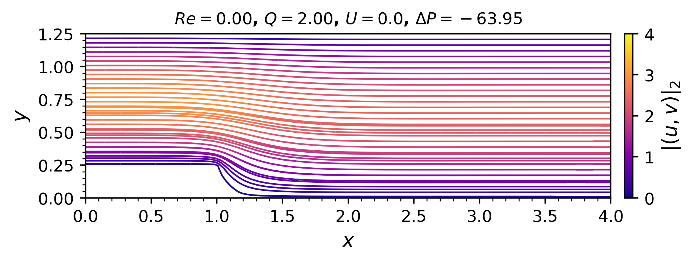
(a) Stokes $\mathcal{H}=1.25$

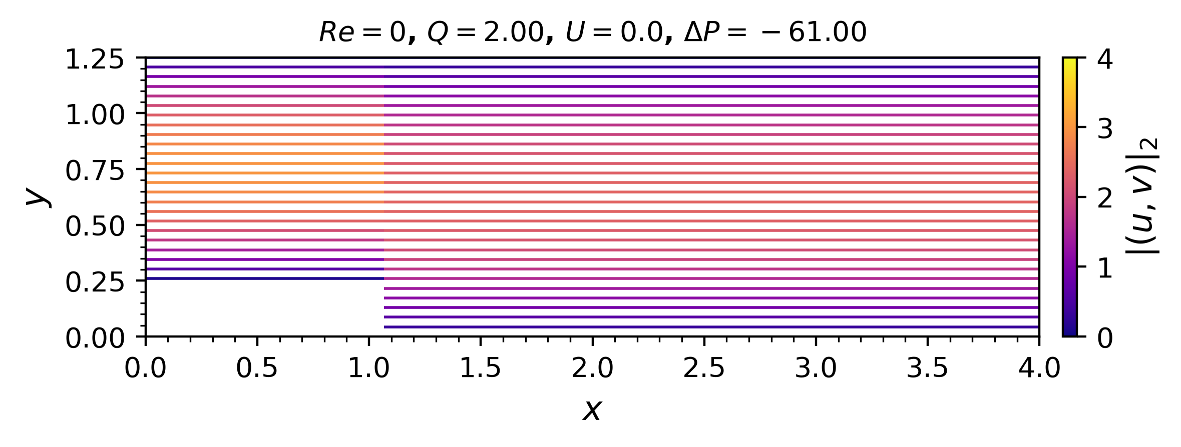
(b) Reynolds $\mathcal{H}=1.25$

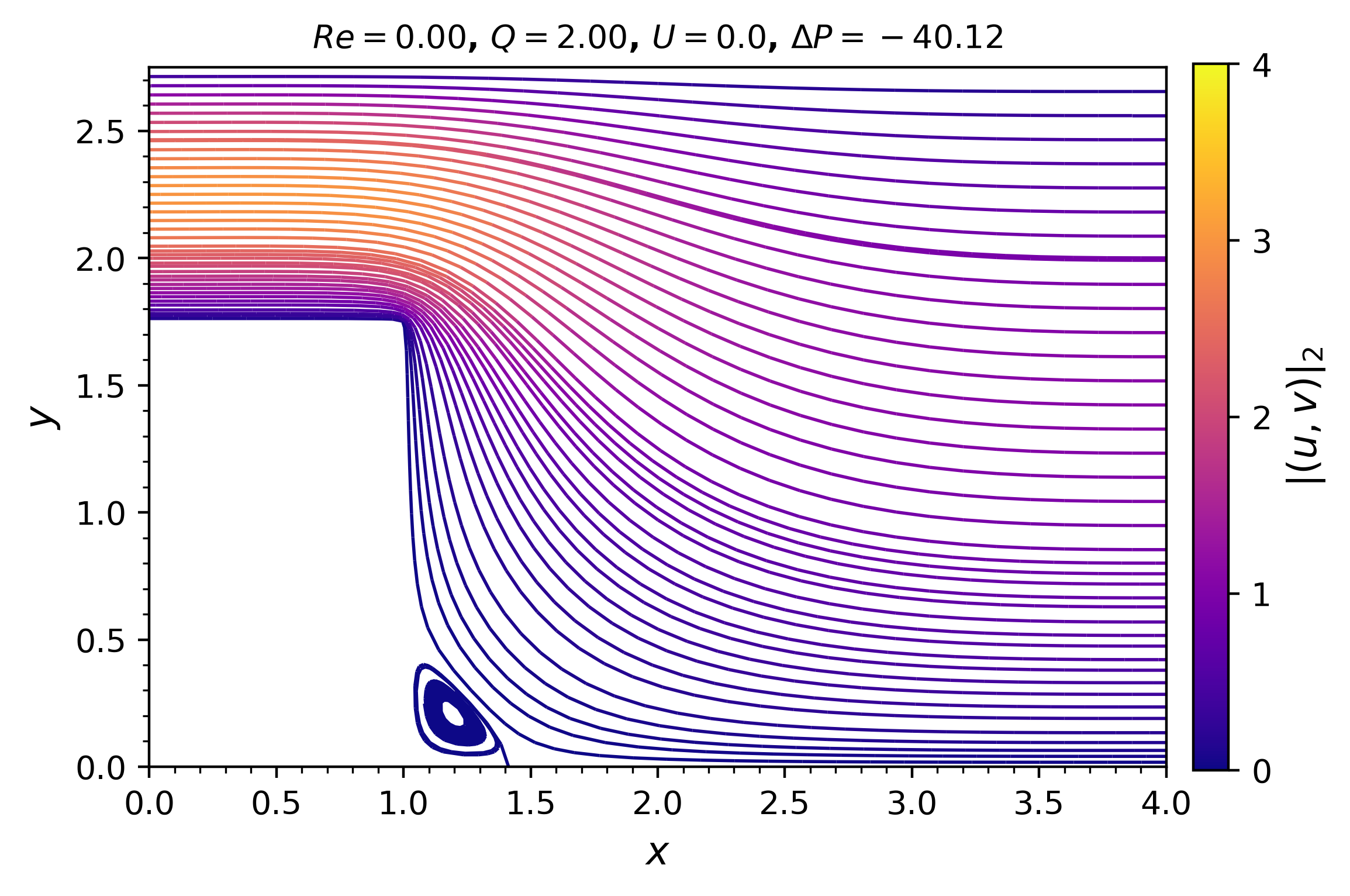
(c) Stokes $\mathcal{H}=2.75$

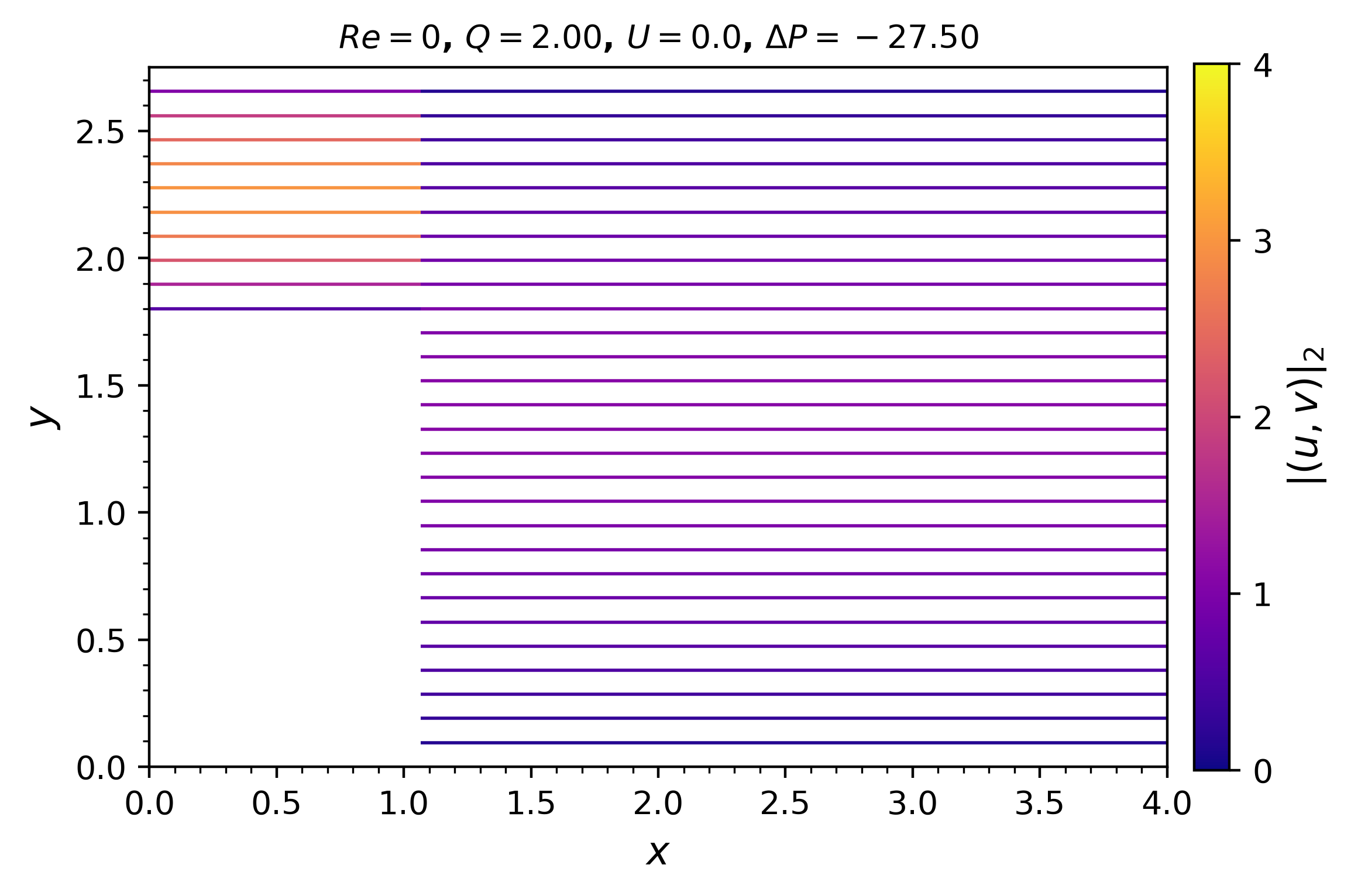
(d) Reynolds $\mathcal{H}=2.75$

Figure 2: Velocity streamlines for the BFS. Stokes solutions capture regions of corner recirculation, increasing in size with expansion ratio $\mathcal{H}$.

Flow separation in the BFS is assessed for various expansion ratios $\mathcal{H}$. The corner separated region is characterized by the separation point $(L_{\text{in}},y_{r})$ and the reattachment point $(L_{\text{in}}+x_{r},0)$. As shown in Fig. 3, the separation and reattachment lengths $y_{r}$ and $x_{r}$ increase steadily with increasing expansion ratio. Close-up views of the corner recirculation in the BFS are shown in Fig. 4. Secondary recirculation zones are captured on zooming closer in to the corner. The size and intensity of each sequential eddy decreases rapidly on approach to the corner.

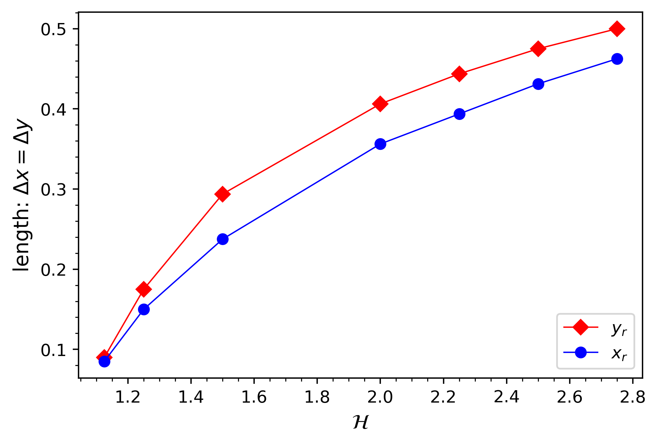
Figure 3: Points of flow separation $(L_{\text{in}},y_{r})$ and reattachment $(L_{\text{in}}+x_{r},0)$ in the BFS, Stokes solutions. The corner recirculation region increases with expansion ratio $\mathcal{H}$.

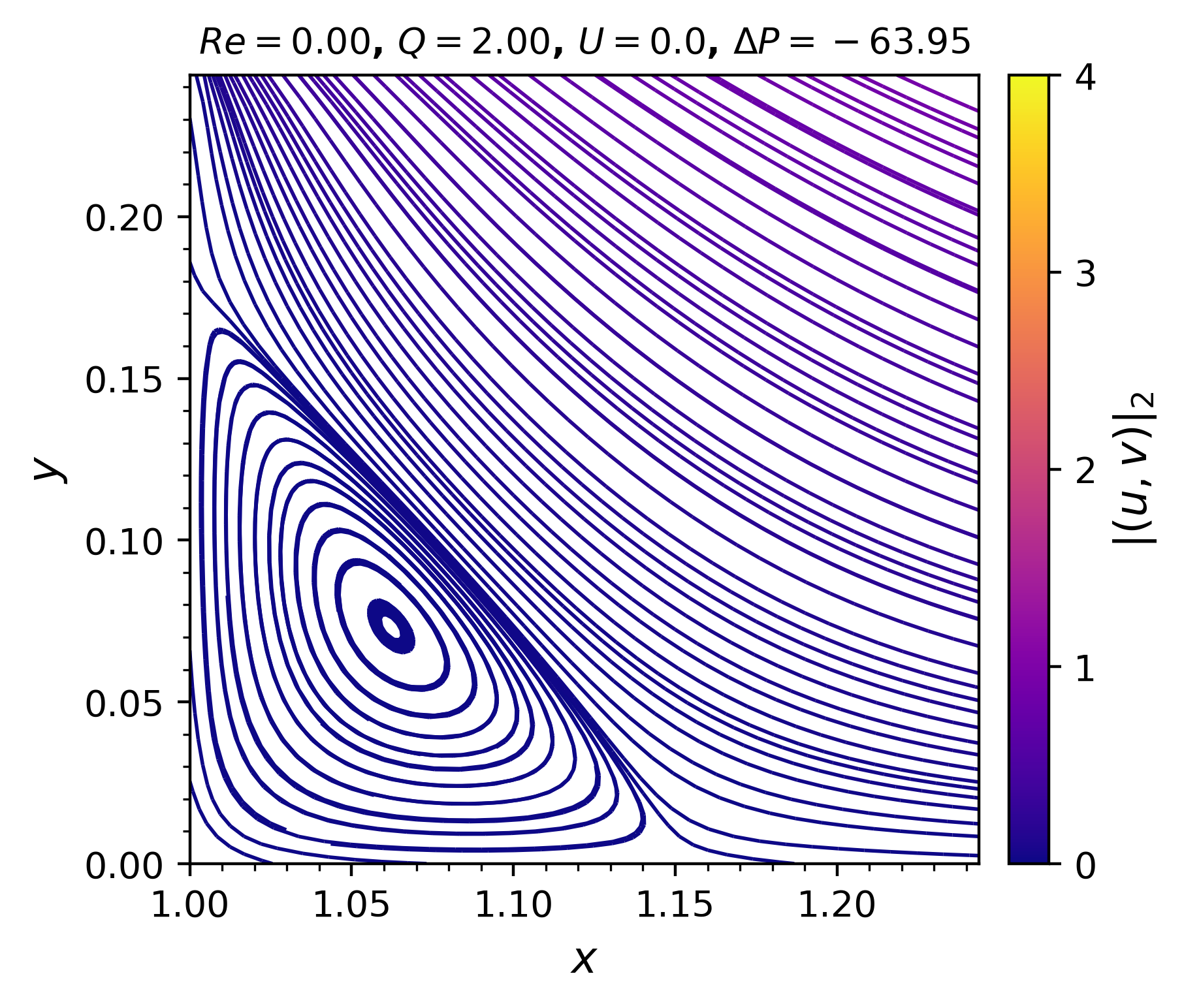
(a) $\mathcal{H}=1.25$

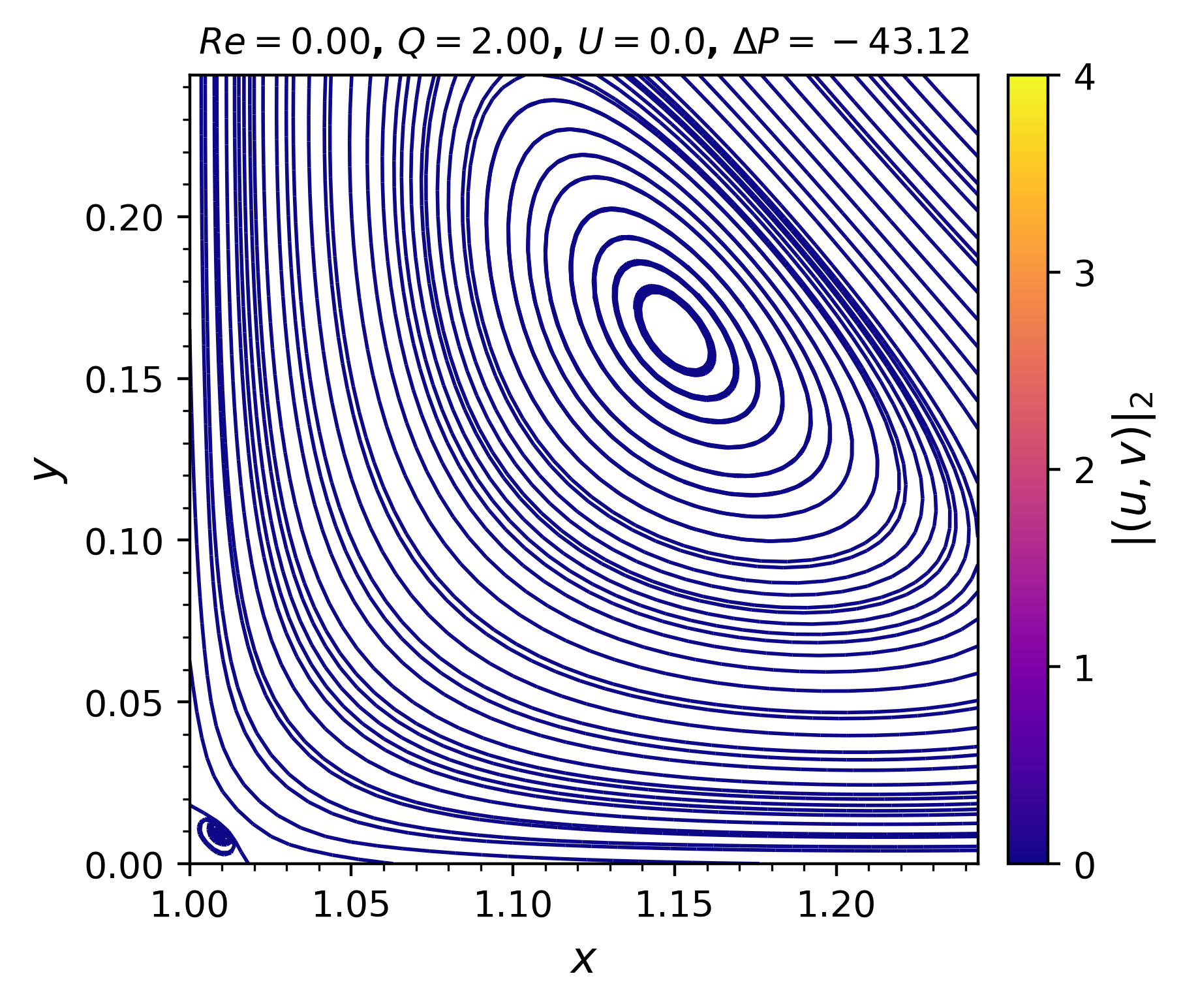
(b) $\mathcal{H}=2$

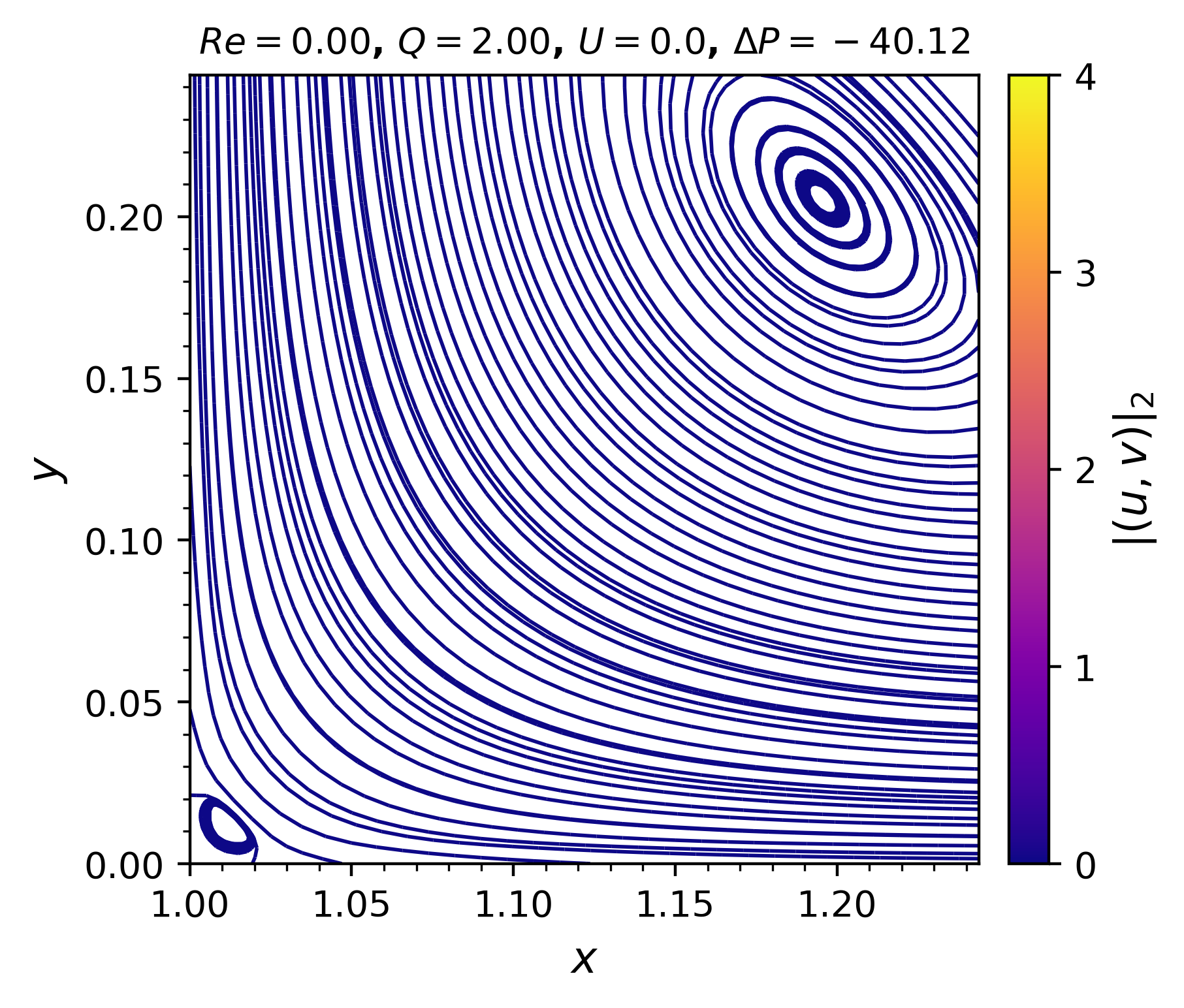
(c) $\mathcal{H}=2.75$

Figure 4: Velocity streamlines for the BFS, observing the lower corner, Stokes solutions. Secondary recirculation is observed at larger expansion ratios $\mathcal{H}$.

The pressure contours for the Reynolds and Stokes solutions to the BFS are shown in Fig. 5. As the expansion ratio $\mathcal{H}$ increases, the pressure drop $\Delta\mathcal{P}$ is less extreme. The pressure contours in the vicinity of the step tip with Stokes solution are shown in Fig. 6; in this region the pressures from the Reynolds and Stokes solutions vary significantly. In the Stokes solutions, the minimum pressure occurs at or immediately after the step tip; the corresponding Reynolds solutions all achieve their minimum pressure at the outlet. The spiraling pressure contours in the Stokes solutions indicate that pressure gradients $\frac{\partial p}{\partial y}$ and $\frac{\partial p}{\partial x}$ are of proportional magnitude in the vicinity of the step.

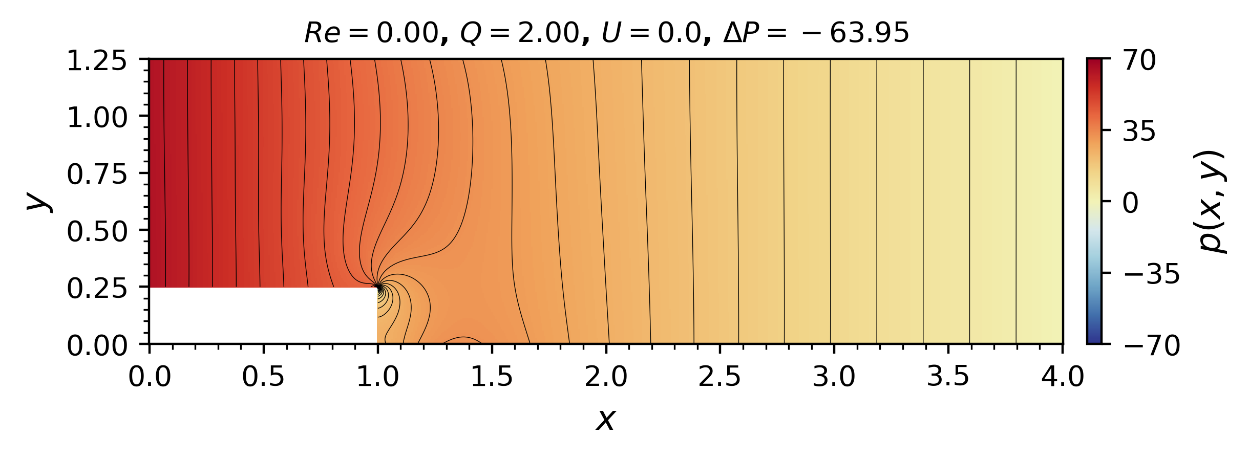
(a) Stokes $\mathcal{H}=1.25$

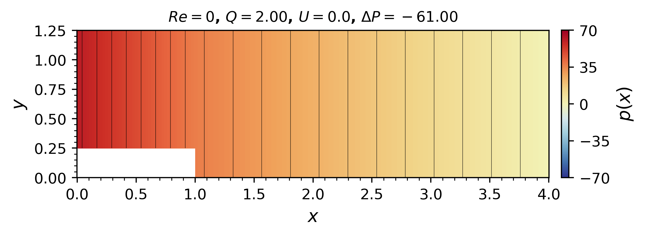
(b) Reynolds $\mathcal{H}=1.25$

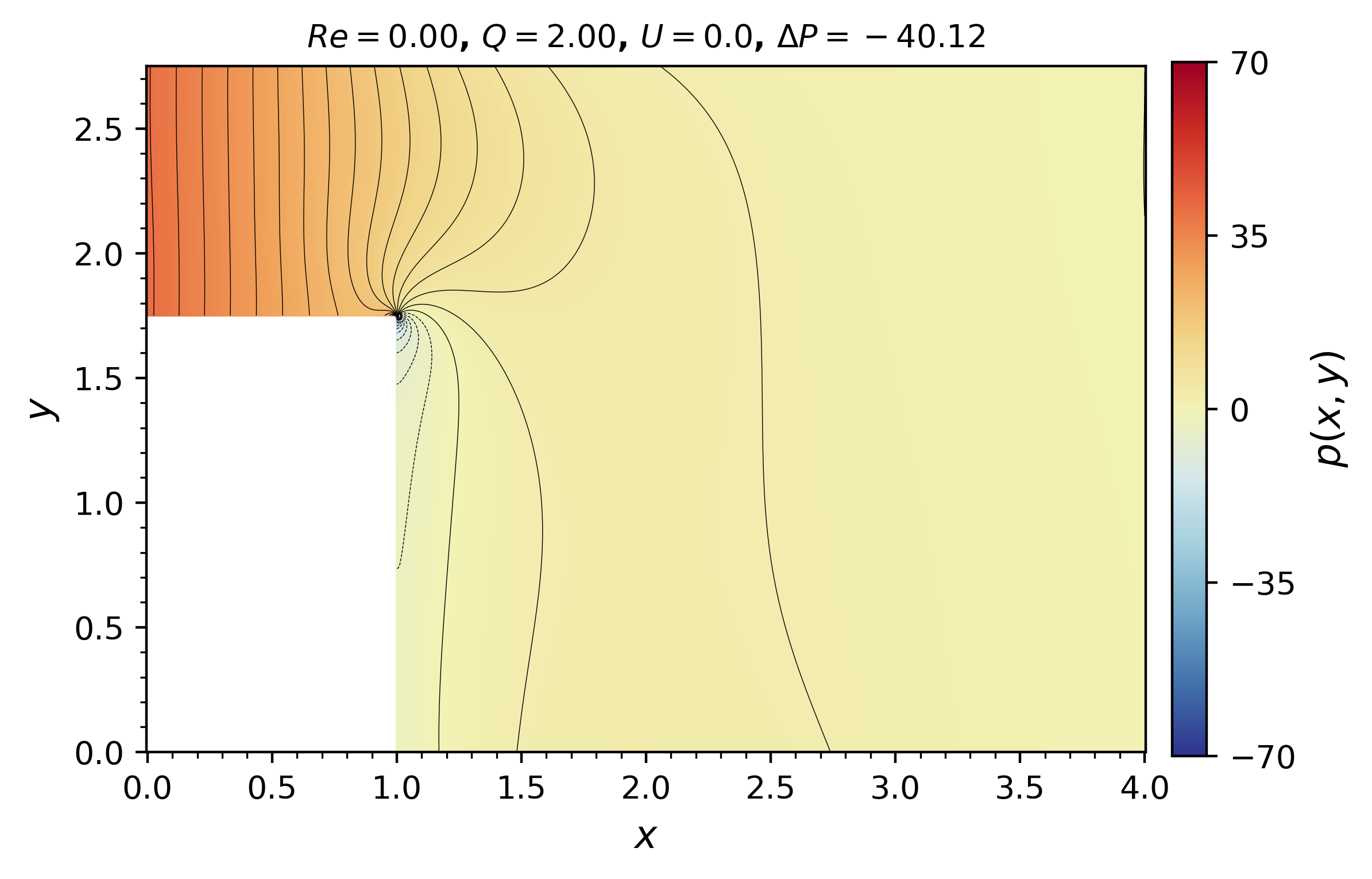
(c) Stokes $\mathcal{H}=2.75$

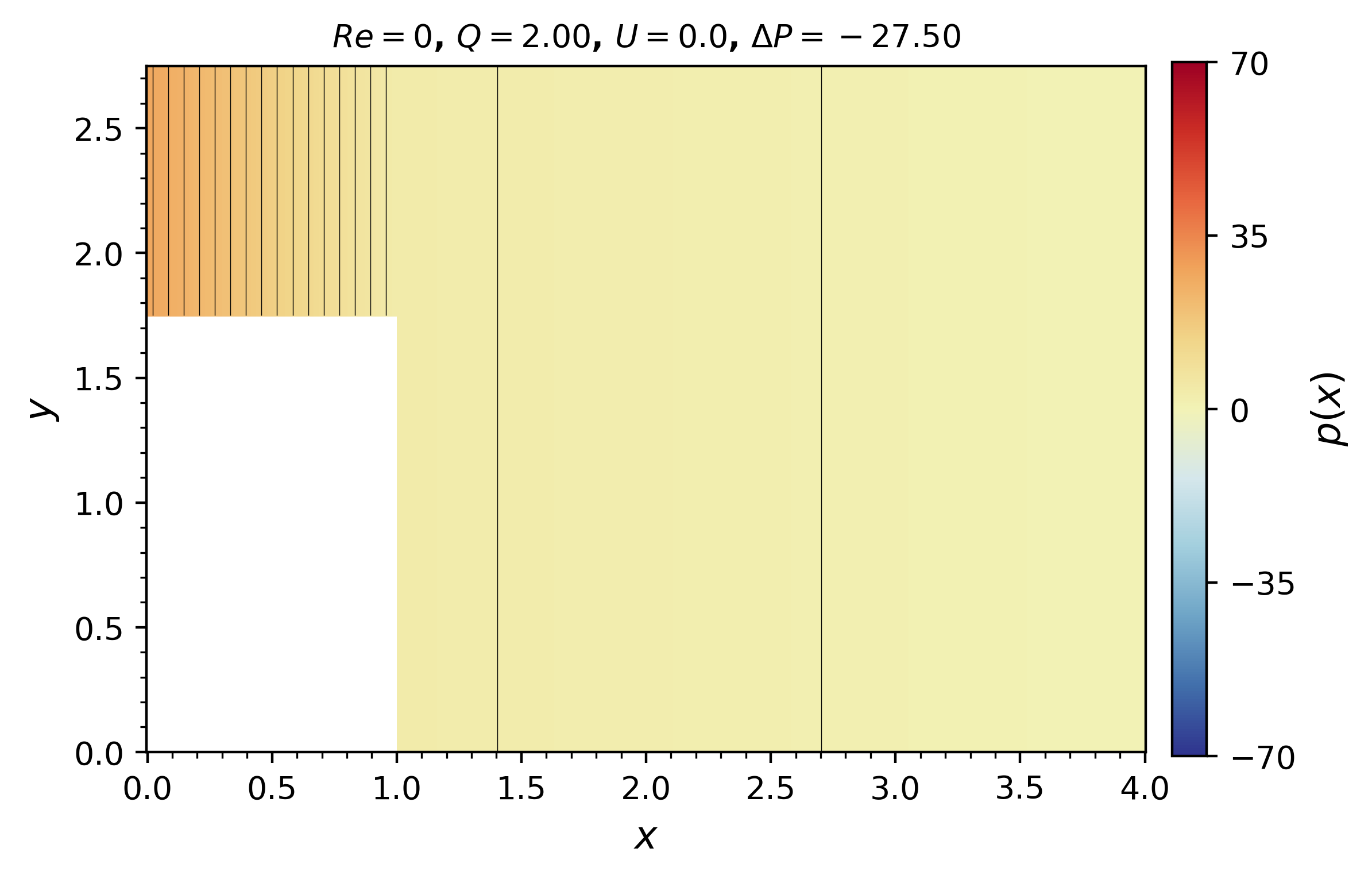
(d) Reynolds $\mathcal{H}=2.75$

Figure 5: Pressure contours for the BFS. Curved contours in the Stokes solutions indicate significant pressure gradients at the step. The pressure drop $\Delta\mathcal{P}$ is more extreme at smaller expansion ratios $\mathcal{H}$. For a particular $\mathcal{H}$, $\Delta P$ is less extreme in the Reynolds solution versus the Stokes solution.

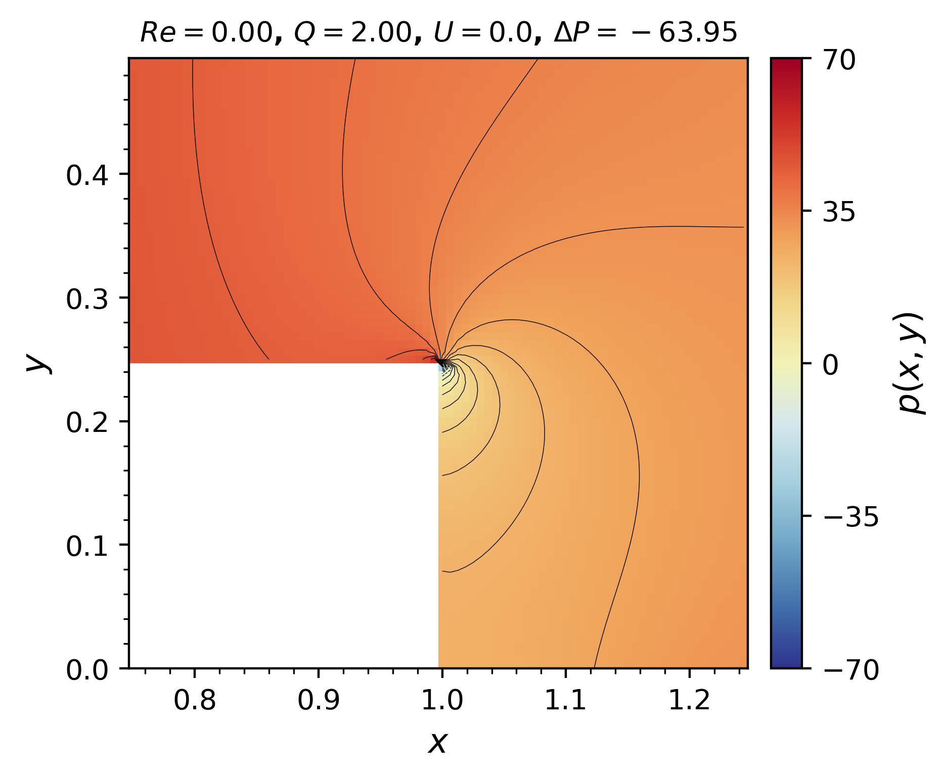
(a) $\mathcal{H}=1.25$

(b) $\mathcal{H}=2$

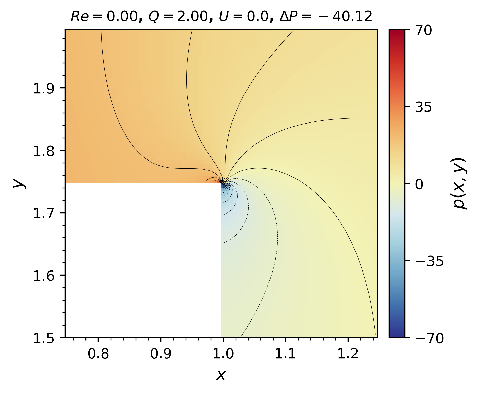
(c) $\mathcal{H}=2.75$

Figure 6: Pressure contours for the BFS, observing the step tip, Stokes solutions. Maximum and minimum pressure occur on the lower surface before and after the step.

The resistance $\mathcal{R}=-\Delta\mathcal{P}/\mathcal{Q}$ for the BFS decreases with increasing expansion ratio $\mathcal{H}$, see Fig. 7. The Reynolds solutions consistently report a lower resistance than the Stokes solutions: the Reynolds solutions do not accurately account for pressure losses at the step, leading to a less extreme pressure drop $\Delta\mathcal{P}$ for the same flux $\mathcal{Q}$. Moreover, the relative error in resistance between the Reynolds and Stokes solutions $|\mathcal{R}_{\text{Reyn.}}-\mathcal{R}_{\text{Stokes}}|/|\mathcal{R}_{\text{Stokes}}|$ increases with increasing expansion ratio. At $\mathcal{H}=1.5$, the relative error has surpassed 10 percent. As the expansion ratio increases relative to the domain length $L$, the step discontinuity has a more significant impact.

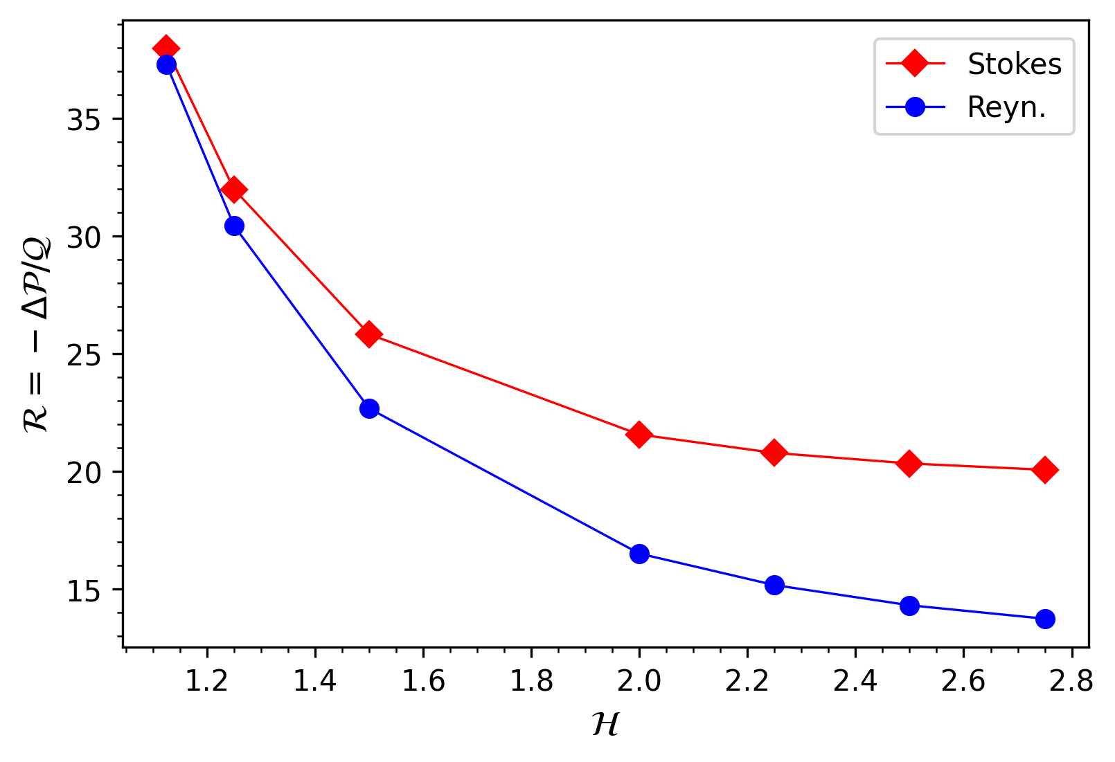
(a) Resistance

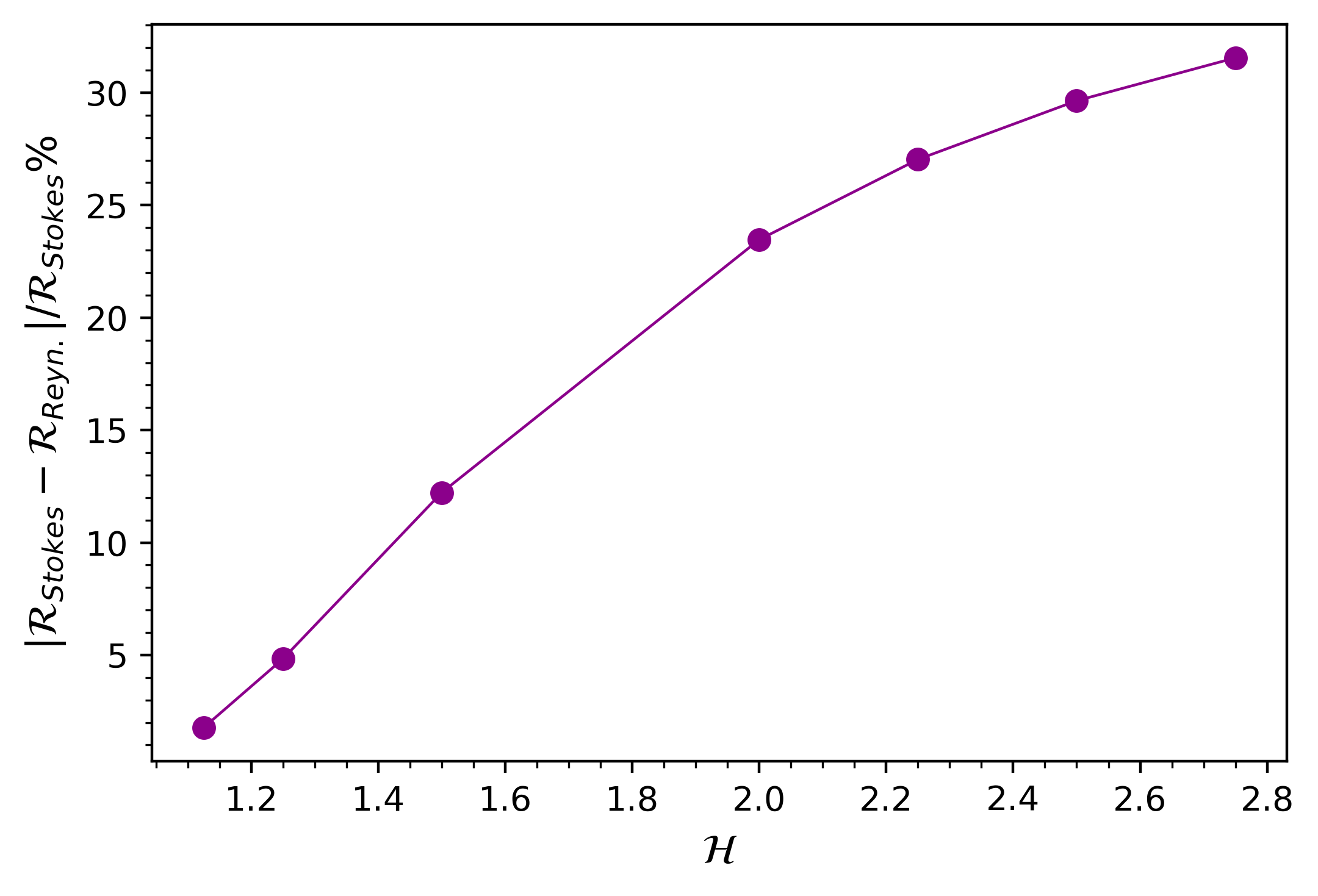
(b) Resistance $\%$-error

Figure 7: In the BFS, the fluid resistance $\mathcal{R}$ for the Reynolds and Stokes solutions decreases with increasing expansion ratio $\mathcal{H}$. The Reynolds solutions underestimate $\mathcal{R}$, the relative error in $\mathcal{R}$ increases with increasing $\mathcal{H}$.

4.2 Recirculation in wedged corners

This section presents a variation of the BFS, inspired by our investigation of corner recirculation. We similarly consider an expansion ratio $\mathcal{H}=H_{\text{out}}/H_{\text{in}}$ for the step; now the lower corner downstream of the step is smoothed by a wedge to occlude the recirculation zone that occurs in the standard BFS. The film height is given by,

(55) $$h(x)=\begin{cases}H_{\text{in}}&0\leq x\leq L_{\text{in}}\\ H_{\text{out}}-\frac{\delta_{y}}{\delta_{x}}(L_{\text{in}}+\delta_{x}-x)&L_{\text{in}}\leq x\leq L_{\text{in}}+\delta_{x}\\ H_{\text{out}}&L_{\text{in}}+\delta_{x}\leq x\leq L\end{cases},$$

a schematic is shown in Fig. 8. We compare the Reynolds and Stokes solutions to the wedged corner BFS and standard BFS for varying expansion ratios $1<\mathcal{H}\ll L$, and corner wedges of height $0\leq\delta_{y}<H_{\text{out}}-H_{\text{in}}$ and length $0\leq\delta_{x}\ll L$. Results are presented for various $H_{\text{out}}$ with $H_{\text{in}}=1$, $L_{\text{in}}=1$ and $L=4$.

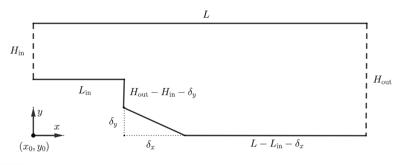
Figure 8: Schematic of the wedged corner BFS with expansion ratio $\mathcal{H}=H_{\text{out}}/H_{\text{in}}$, wedge height $\delta_{y}$ and length $\delta_{x}$.

First, we consider the wedge height $\delta_{y}=y_{r}$ and length $\delta_{x}=x_{r}$ equal to the flow separation and reattachment points determined through results of Section 4.1. With this construction, we observe the effect of smoothing the corner recirculation.

The Stokes solutions of pressure and velocity for the wedged corner BFS at $\mathcal{H}=2$, $\delta_{y}=y_{r}=0.41$, and $\delta_{x}=x_{r}=0.35$ are presented in Fig. 9 alongside the standard BFS solution for $\mathcal{H}=2$. In each standard BFS example, we observe that the solutions of velocity and pressure are very close to those in the wedged corner counterpart example. The maximum percent relative error in $\Delta\mathcal{P}$ we encounter is 0.125% for $\mathcal{H}=2.75$, which is the extremal expansion ratio we consider for $L=4$. Likewise, the percent error in resistance between the Reynolds and Stokes solutions do not change significantly for the wedged corner BFS versus the standard BFS.

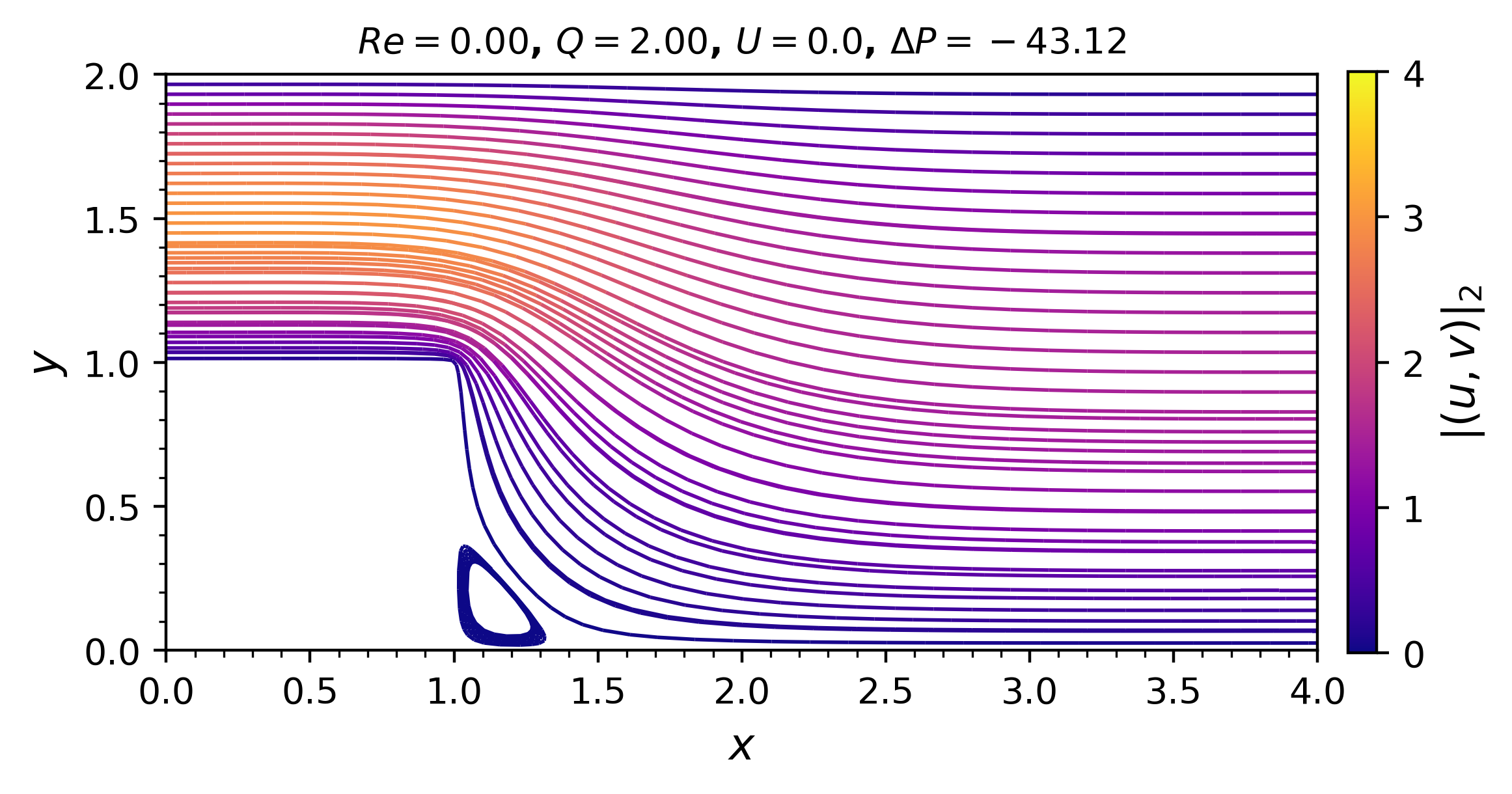
(a) BFS velocity

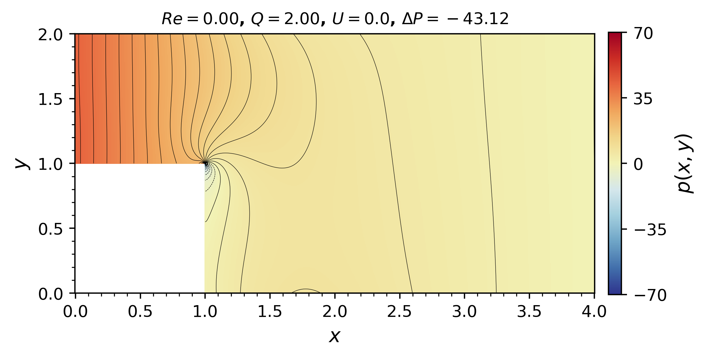
(b) BFS pressure

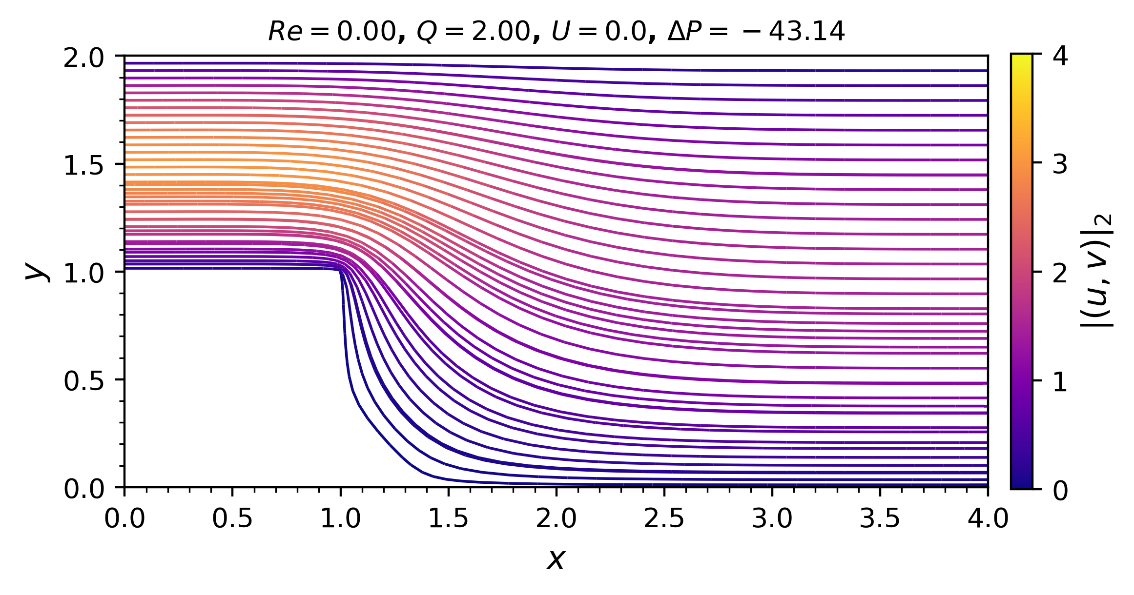
(c) Wedged corner BFS velocity

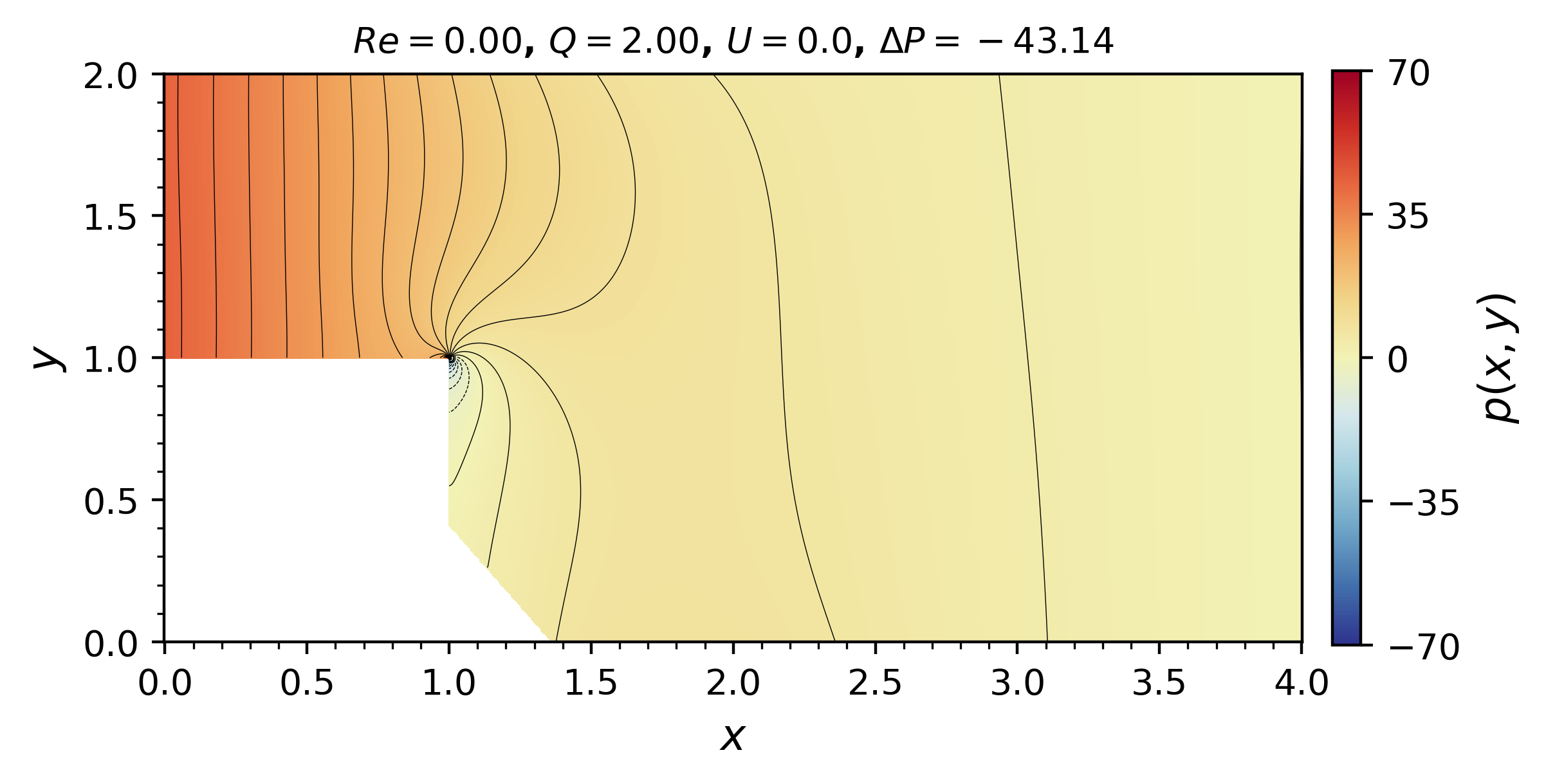
(d) Wedged corner BFS pressure

Figure 9: BFS and wedged corner BFS, Stokes solutions, $\mathcal{H}=2$, $\delta_{x}=x_{r}=0.36$, $\delta_{y}=y_{r}=0.41$. The velocity and pressure profiles are very similar with and without the wedged corner.

Now we analyze the effect of resizing the corner wedge. For each expansion ratio $\mathcal{H}$ with separation and reattachment lengths $y_{r}$ and $x_{r}$, consider the class of examples with wedge length $\delta_{x}\to 0$ and fixed wedge slope $\delta_{y}/\delta_{x}=y_{r}/x_{r}$. Fig. 10 depicts the velocity in the vicinity of the wedged corner for various $\delta_{x}$ with $\mathcal{H}=2$ and $y_{r}/x_{r}\simeq 1.17$. We observe that the flow separation and reattachment points remain stable as the wedge shrinks. The primary flow retains its structure and recirculation fills the space between the corner wedge and the bulk. The pressure drop $\Delta\mathcal{P}$ in all three cases of Fig. 10 are very close. Furthermore, we observe that many wedge variations $0\leq\delta_{x}\leq x_{r}$ and $0\leq\delta_{y}\leq y_{r}$ exhibit the same pressure drop and resistance for a given expansion ratio. In other words, occluding the recirculation zone in the standard BFS appears to lead to a family of geometries having the same fluid resistance, and in which only the local recirculation region is disturbed.

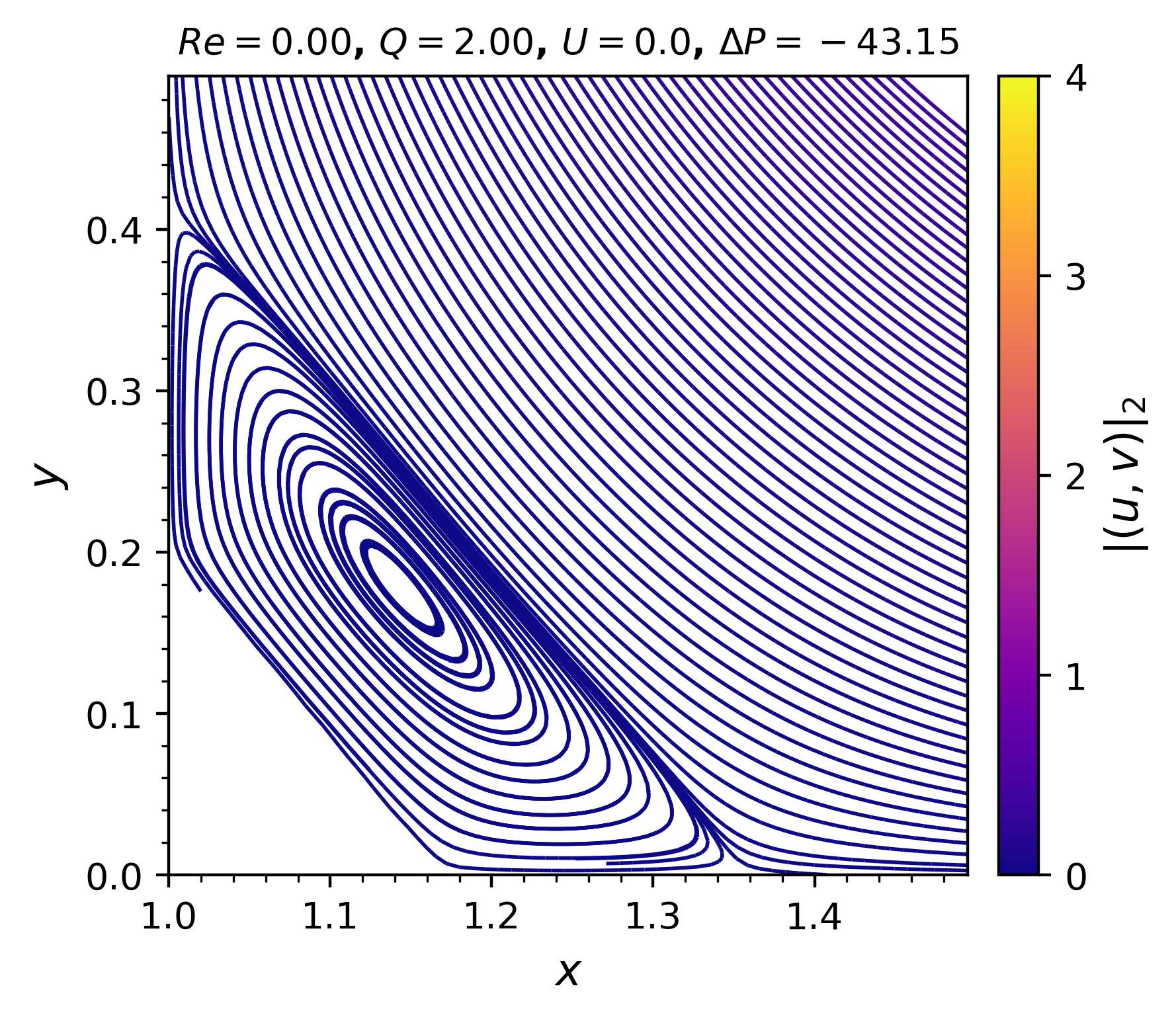
(a) $\delta_{x}=0.15$

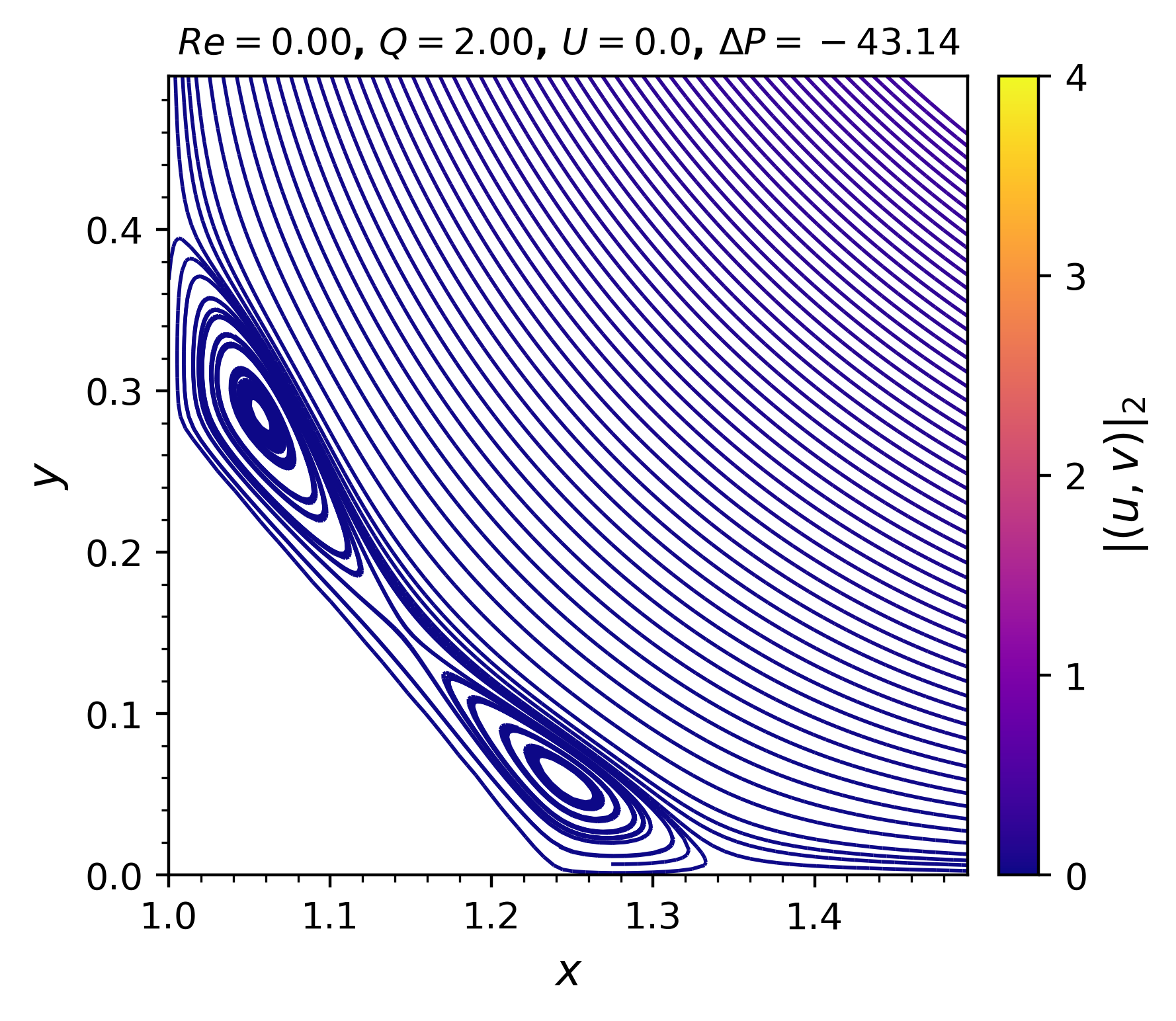
(b) $\delta_{x}=0.25$

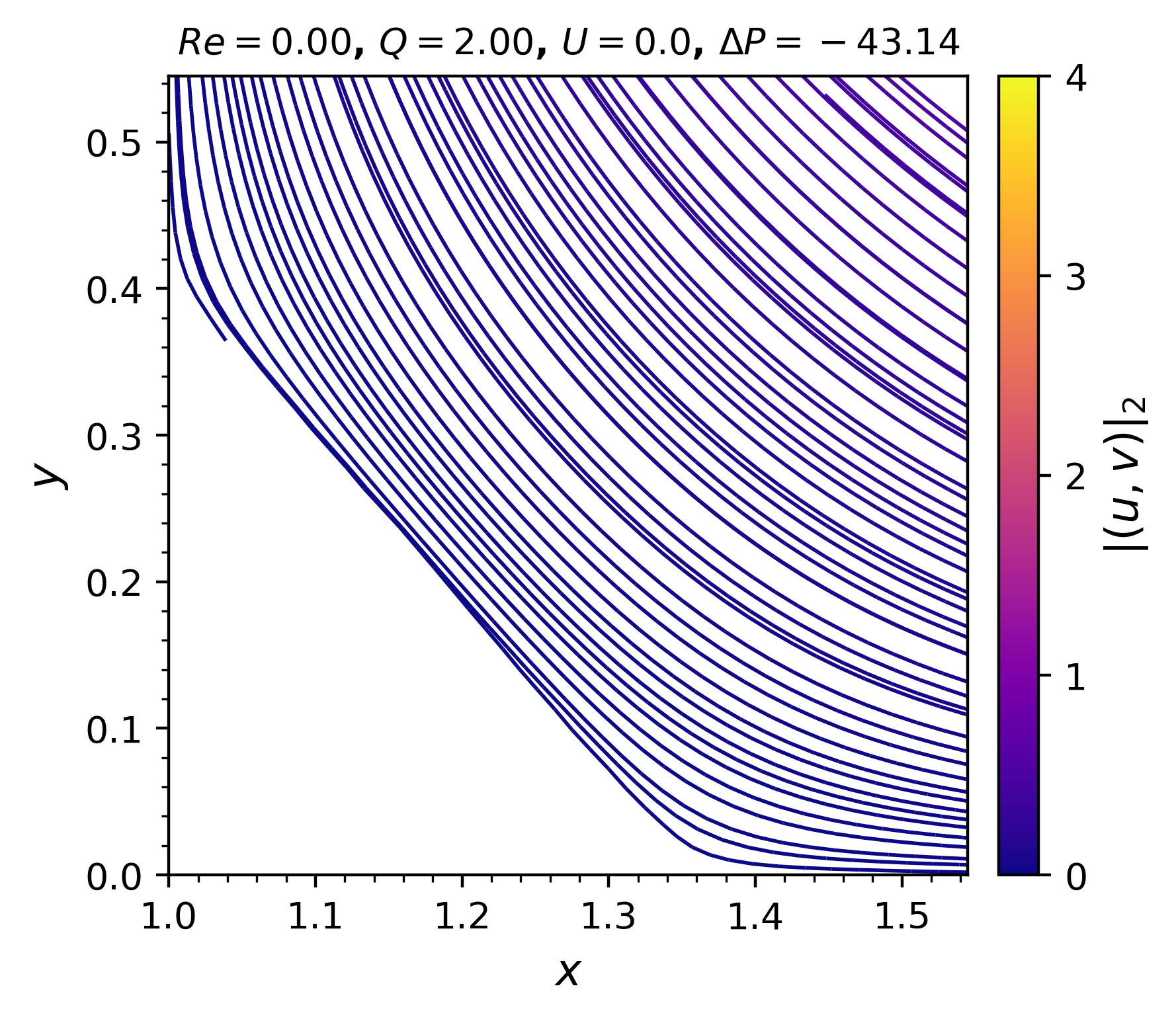
(c) $\delta_{x}=x_{r}=0.36$

Figure 10: Velocity streamlines in the vicinity of the wedged corner, Stokes solutions, $\mathcal{H}=2$, $\delta_{y}/\delta_{x}\simeq 1.17$. Points of flow separation and reattachment are stable as the wedge is retracted, and are consistent with the BFS example of the same $H$.

4.3 A smoothed step bearing

The following section considers a further variation of the BFS. Similar to the BFS and wedge corner variation above, this textured bearing is described by expansion ratio $\mathcal{H}=H_{\text{out}}/H_{\text{in}}$ in a channel of length $L$. Now we additionally smooth the jump in film height ($H_{\text{in}}$ to $H_{\text{out}}$) by a line segment of various slopes, parametrized by the slope reciprocal $\delta$. A schematic of the smoothed step bearing is shown in Fig. 11. The film height is given by,

(56) $$h(x)=\begin{cases}H_{\text{in}}&\hskip 20.00003pt0\leq x\leq\frac{L}{2}-\delta\\ \frac{H_{\text{out}}-H_{\text{in}}}{2}-\frac{H_{\text{out}}-H_{\text{in}}}{\delta}\Big{(}\frac{L}{2}-x\Big{)}&\hskip 20.00003pt\frac{L}{2}-\delta\leq x\leq\frac{L}{2}+\delta\\ H_{\text{out}}&\hskip 20.00003pt\frac{L}{2}+\delta\leq x\leq L\end{cases}.$$

Observe that the limit $\delta\to 0$ achieves a step texture centered at $L/2$.

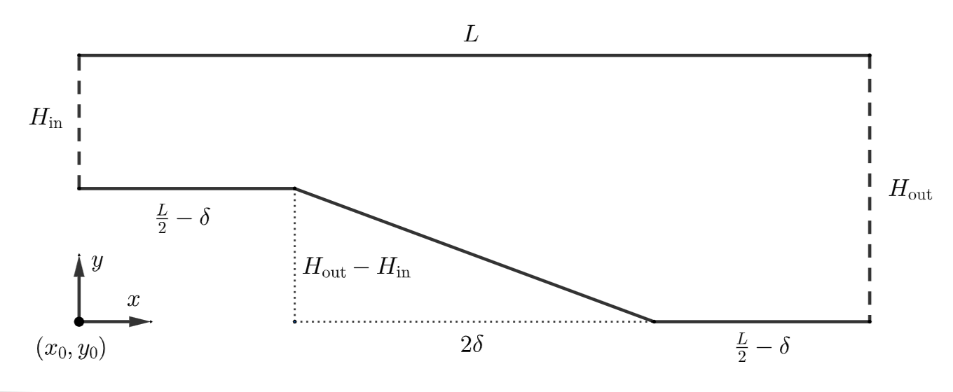
Figure 11: Schematic of the smoothed step bearing with expansion ratio $\mathcal{H}=H_{\text{out}}/H_{\text{in}}$ and slope reciprocal $0\leq\delta\ll\tfrac{L}{2}$.

The Reynolds and Stokes solutions for the smoothed step bearing are evaluated for varying $0\leq\delta\ll L/2$, and a range of expansion ratios $1<\mathcal{H}\ll L$. Results are presented for various $H_{\text{out}}$ and constant $H_{\text{in}}=1$, $L_{\text{in}}=1$, $L=4$. We analyze the error in fluid resistance $\mathcal{R}$ for the Reynolds and Stokes solutions relative to the slope reciprocal $\delta$ and the expansion ratio $\mathcal{H}$.

The velocity streamlines for the Reynolds and Stokes equations are presented in Fig. 12. For sufficiently steep slopes, the Stokes solutions yield flow recirculation in the lower corner whereas the Reynolds solutions do not. Close-up views of the corner recirculation at the base of the slope are shown in Fig. 13. For $\mathcal{H}=2$, flow recirculation is observed for approximately $\delta\leq 0.25$ on grid sizes $\Delta x\sim 0.005$. At all expansion ratios, the size of the recirculation zone increases as $\delta\to 0^{+}$ and the geometry approaches the standard BFS. Notably, at $\delta=0$ the separation and reattachment lengths $y_{r}$ and $x_{r}$ are consistent with those in the BFS examples of the same expansion ratio, despite the inlet and outlet lengths being different.

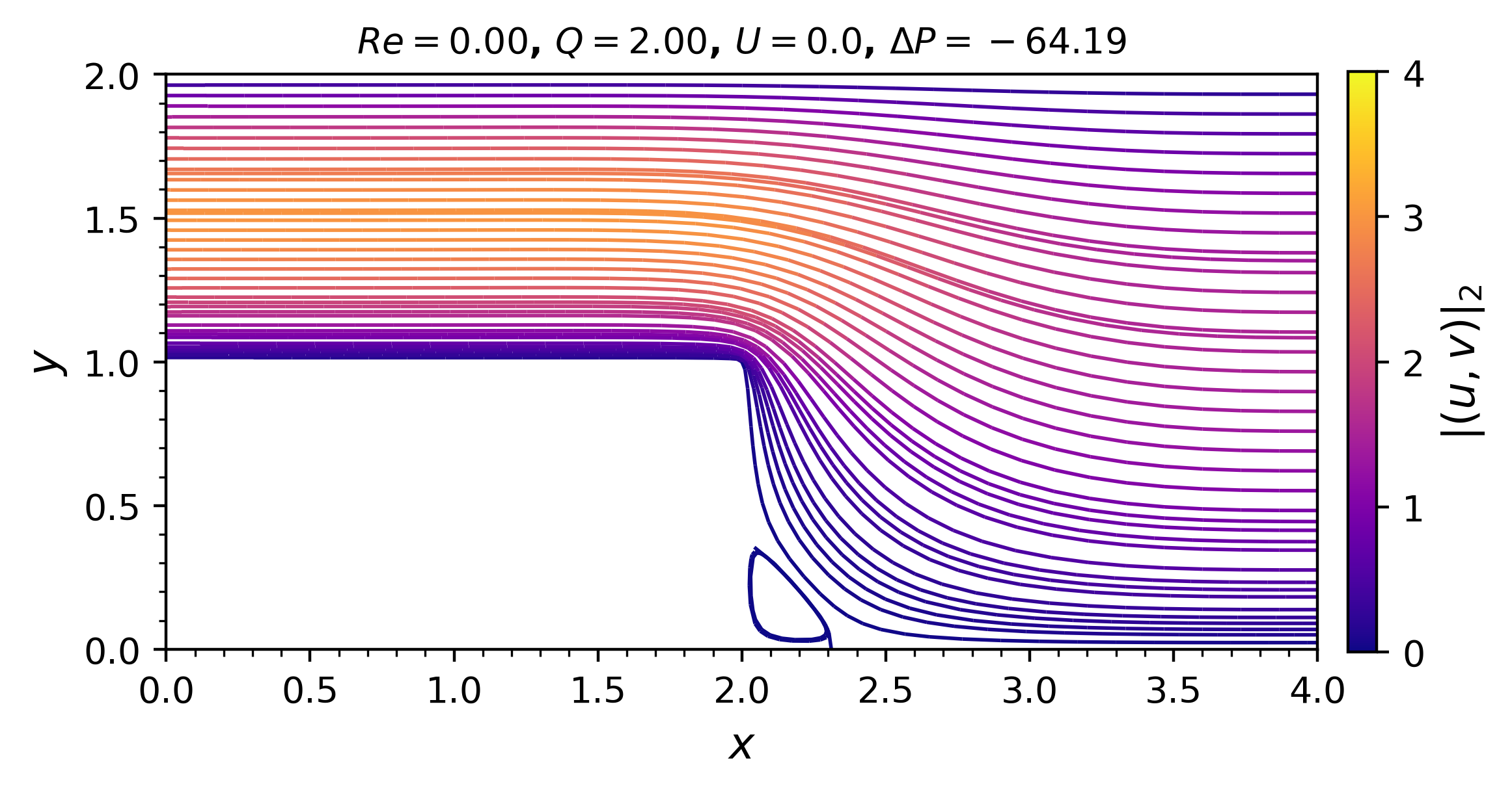
(a) Stokes $\delta=0$

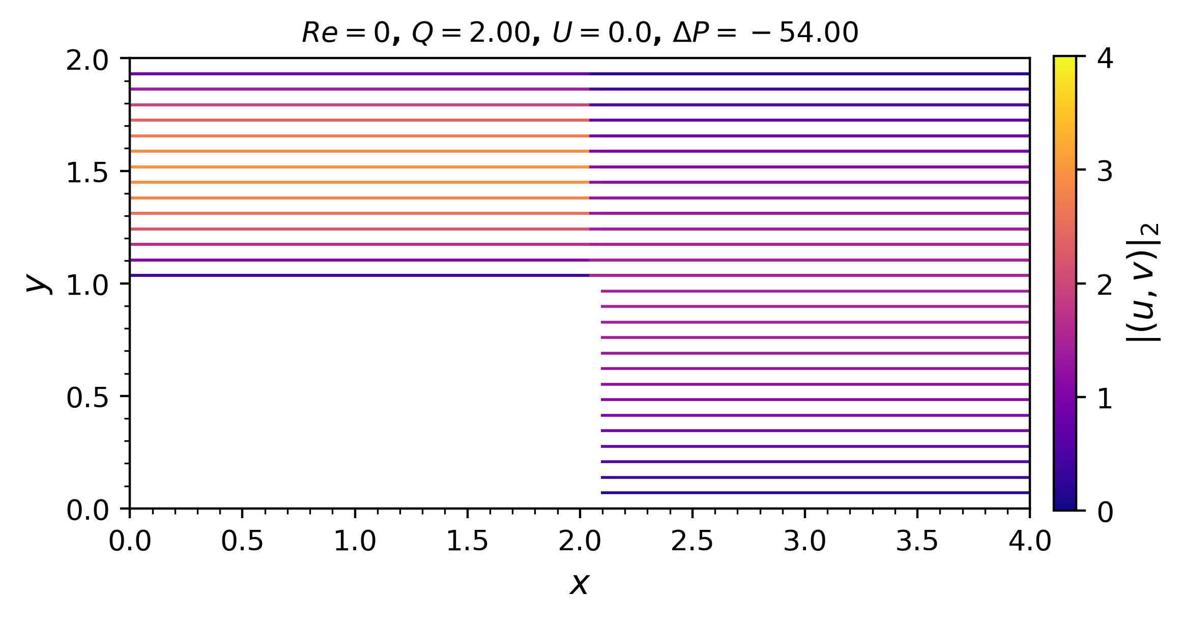
(b) Reynolds $\delta=0$

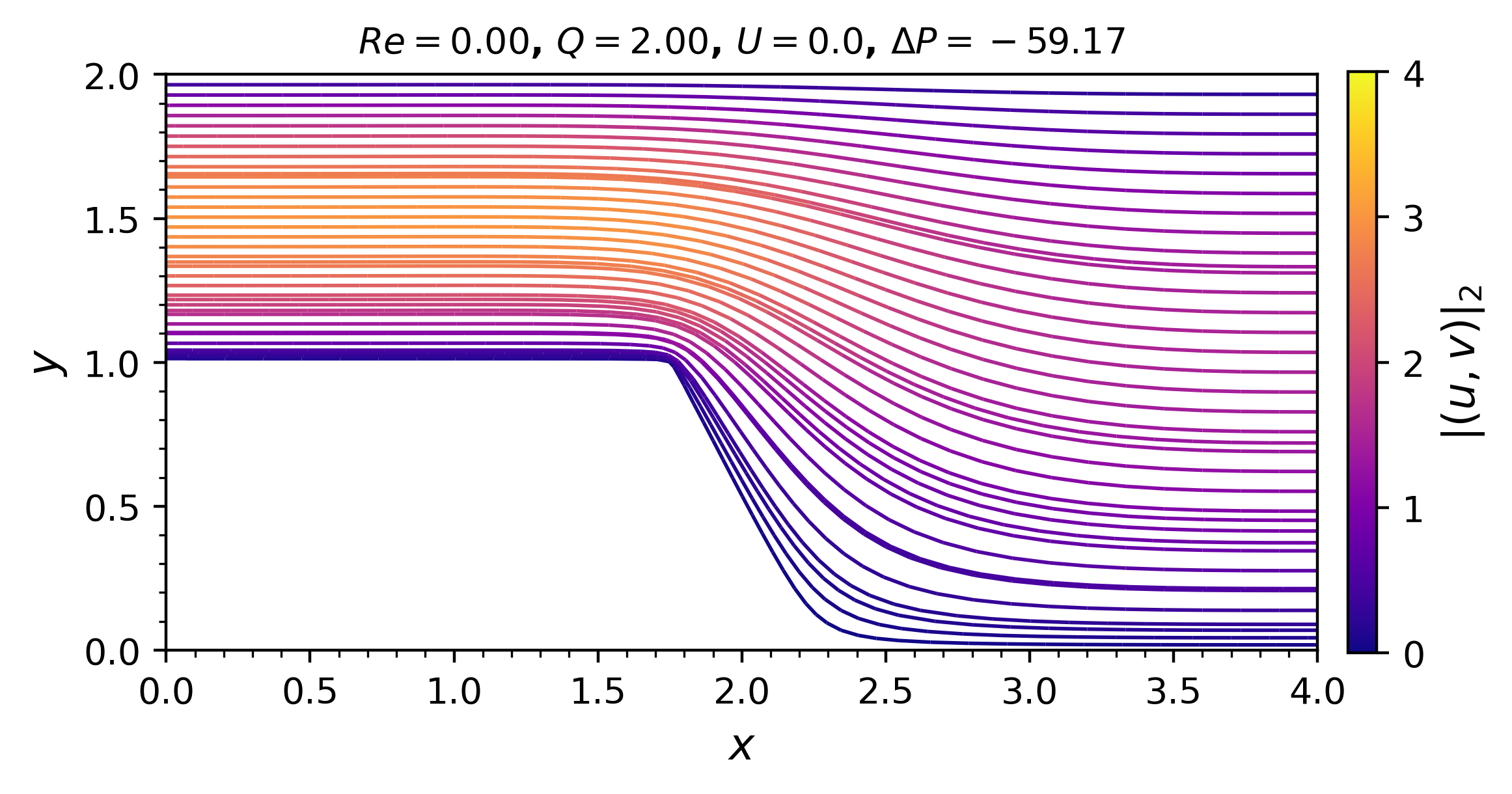
(c) Stokes $\delta=0.25$

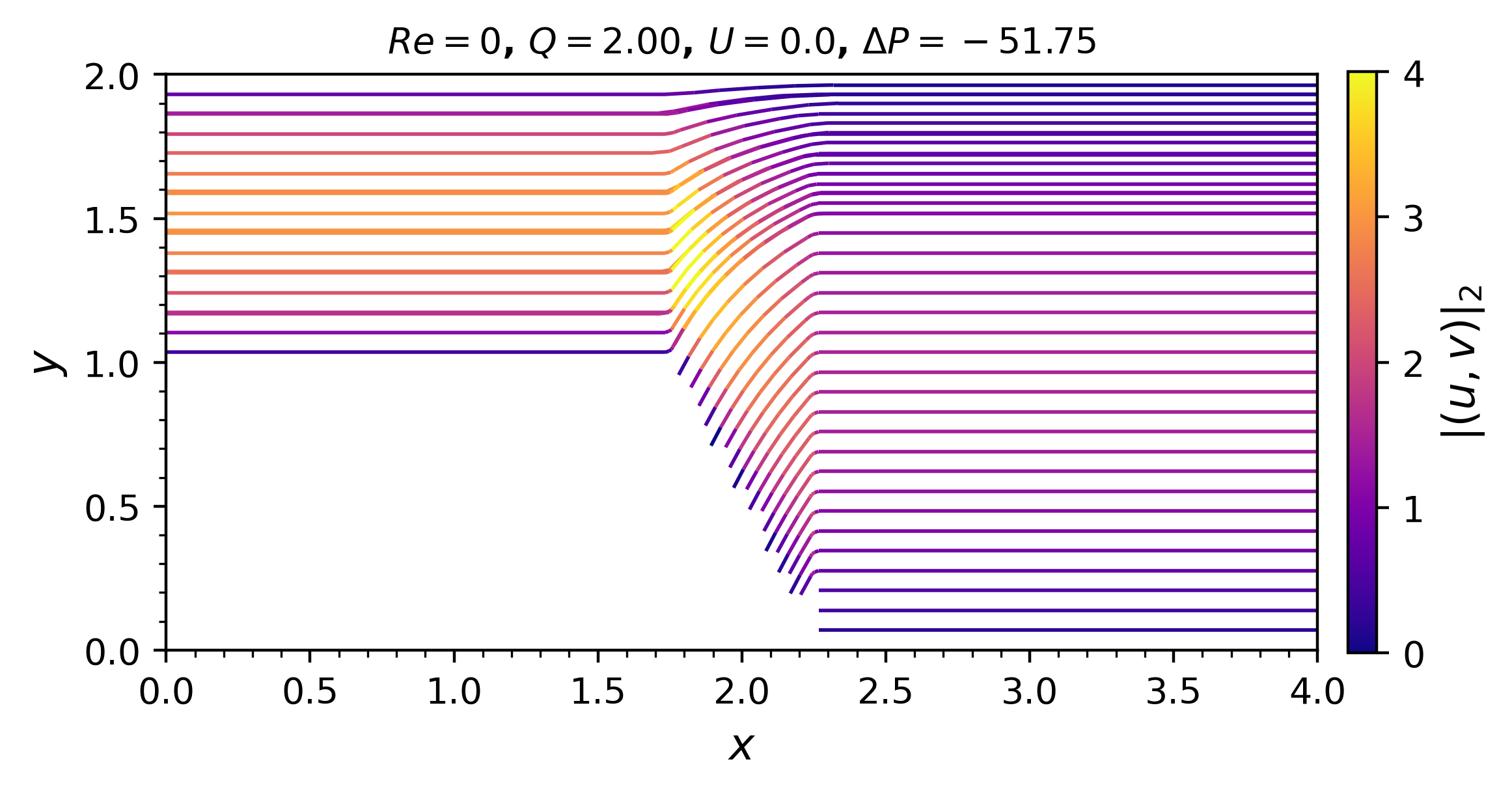
(d) Reynolds $\delta=0.25$

Figure 12: Velocity streamlines for smoothed step bearing, $\mathcal{H}=2$. In the Stokes solutions, recirculation increases as $\delta\to 0^{+}$. In the Reynolds solutions, the magnitude of velocity down the slope is larger than in the corresponding Stokes solution

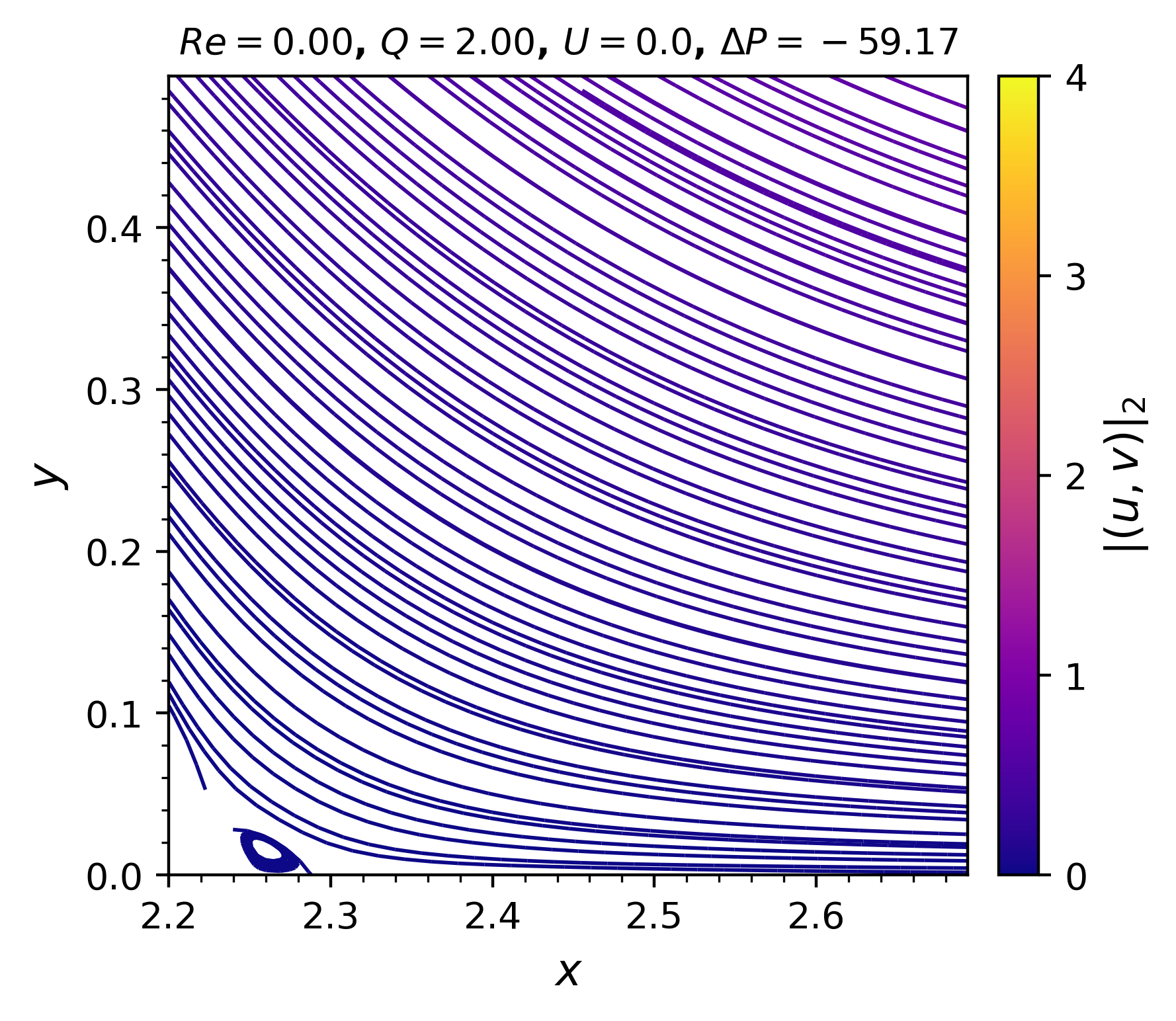
(a) $\delta=0.25$

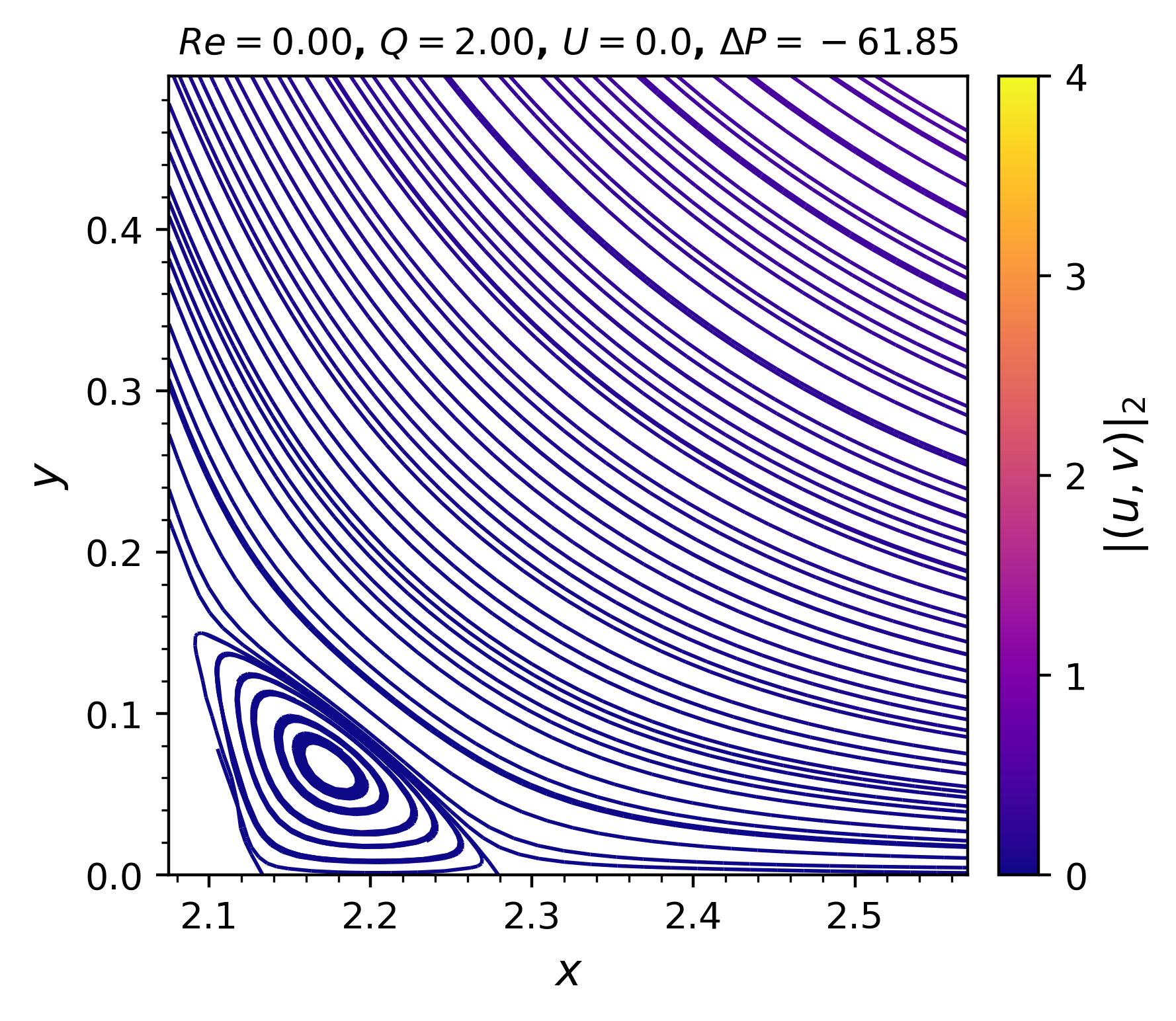
(b) $\delta=0.125$

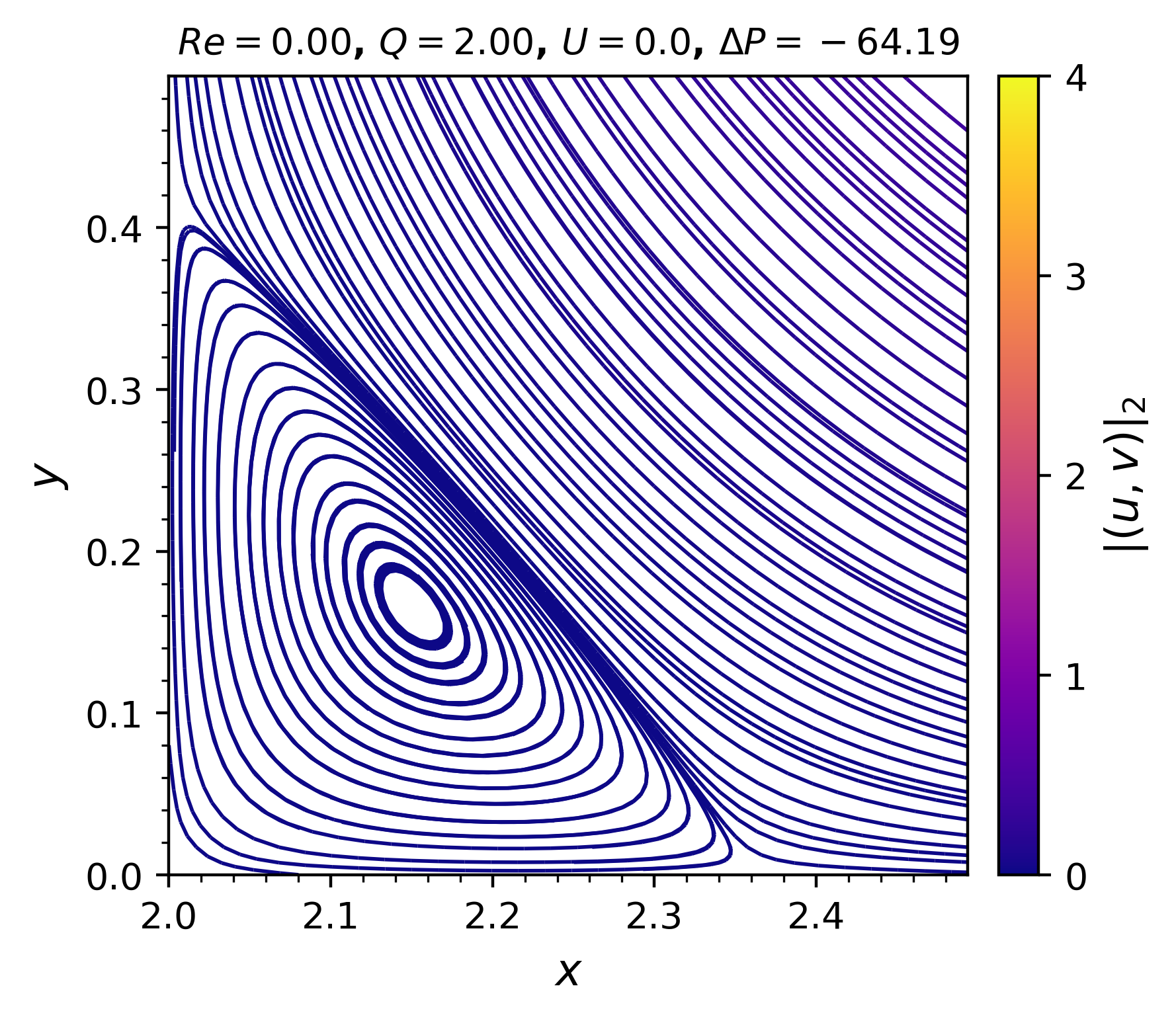
(c) $\delta=0$

Figure 13: Velocity streamlines for the smoothed step bearing observing the base of the slope, $\mathcal{H}=2$, Stokes solutions. Recirculation increases in the step limit $\delta\to 0^{+}$.

The pressure contours for the Reynolds and Stokes solutions are shown in Fig. 14. In the step limit of $\delta\to 0^{+}$, the pressure drop $\Delta P$ is more extreme. For larger $\delta$, approximately $\delta\geq 0.5$ at $\mathcal{H}=2$, the minimum pressure of both the Reynolds and Stokes solutions occur at the outlet. For smaller $\delta$, the Stokes solutions change and obtain their minimum pressure at the step. These observations are consistent with results for the BFS in that both $\frac{\partial p}{\partial y}$ and $\frac{\partial p}{\partial x}$ are significant in the vicinity of the large surface gradient.

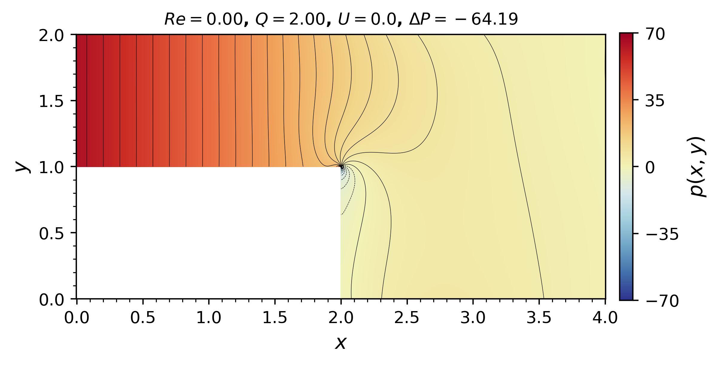
(a) Stokes $\delta=0$

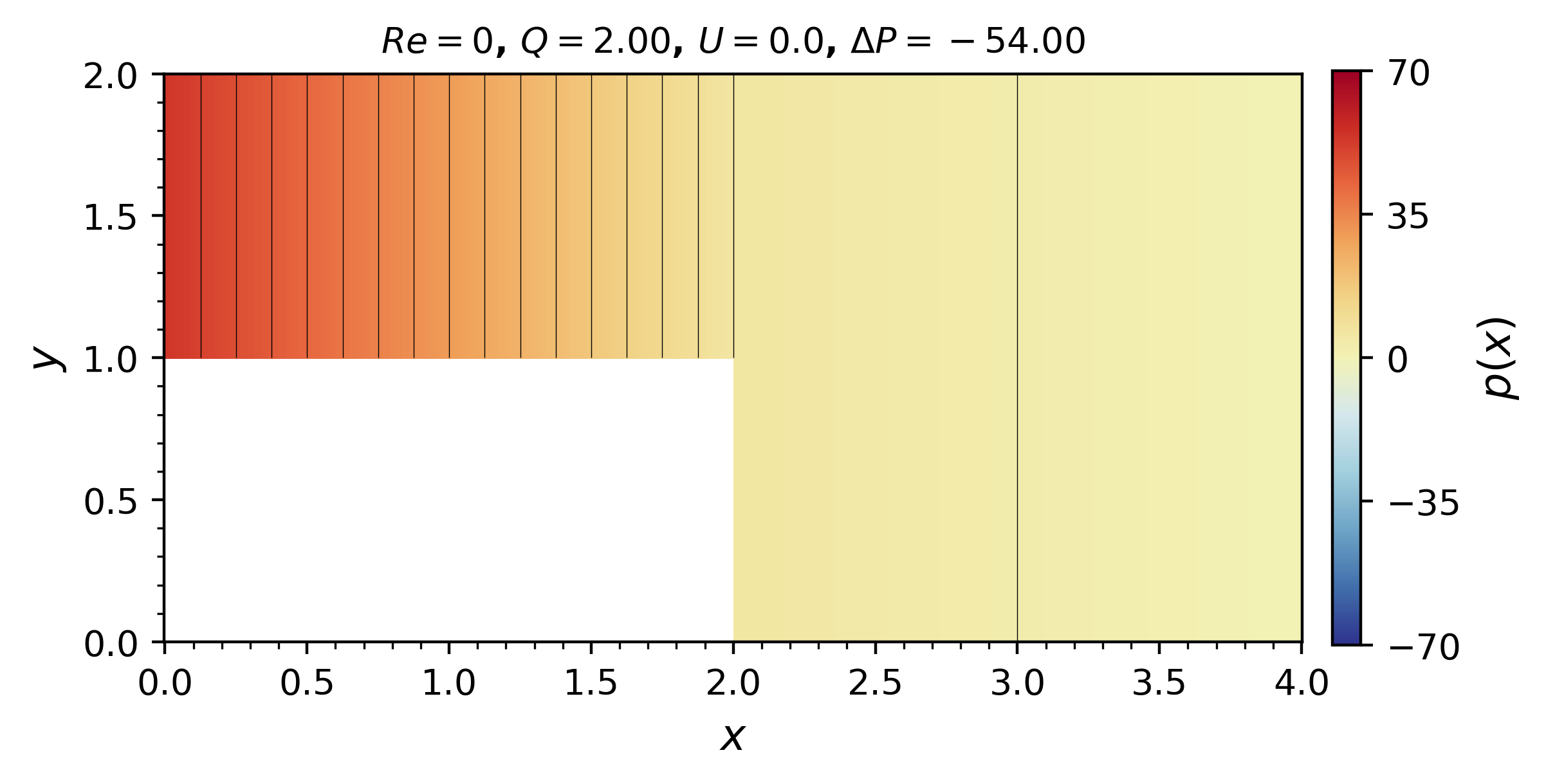
(b) Reynolds $\delta=0$

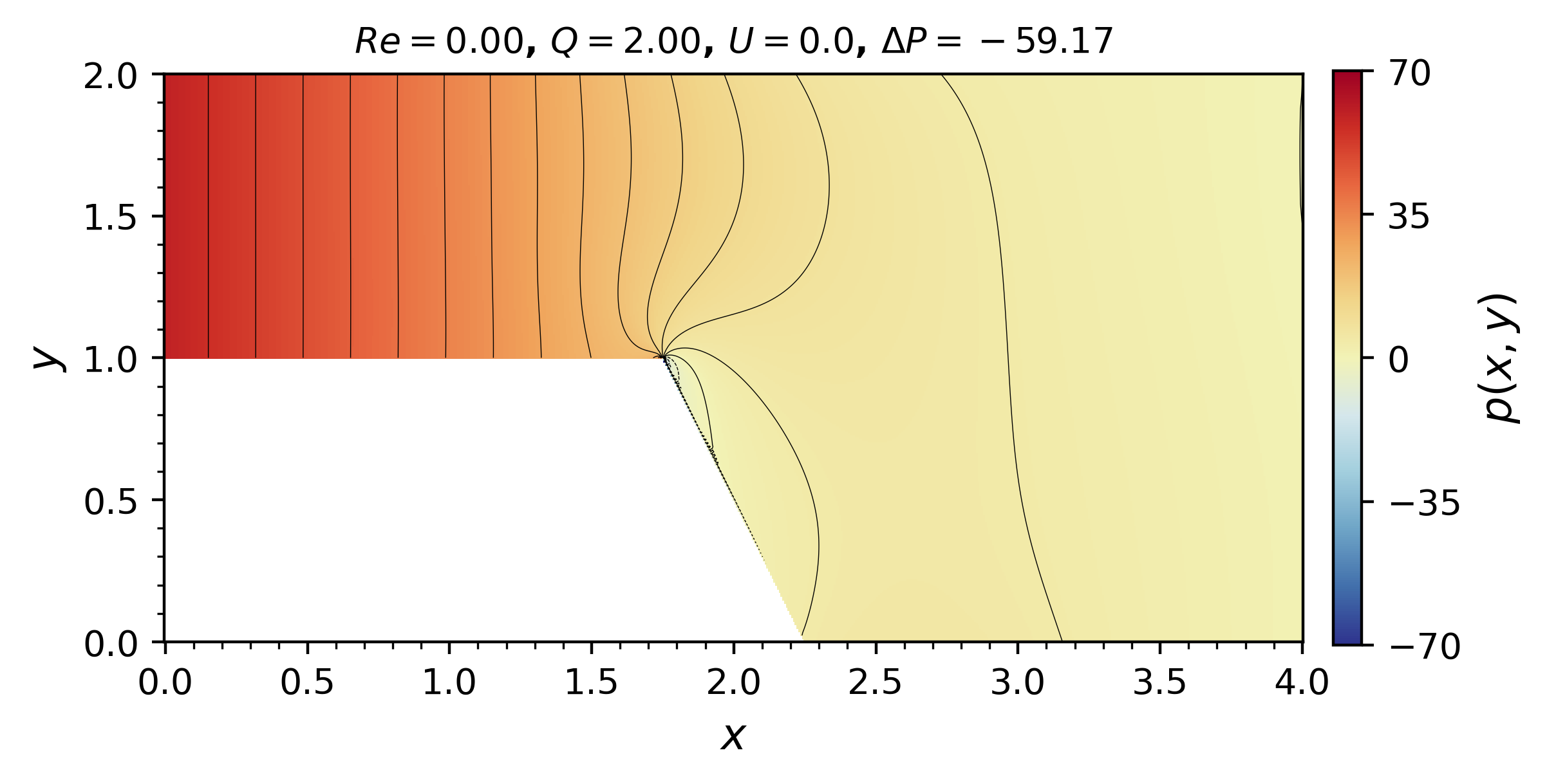
(c) Stokes $\delta=0.25$

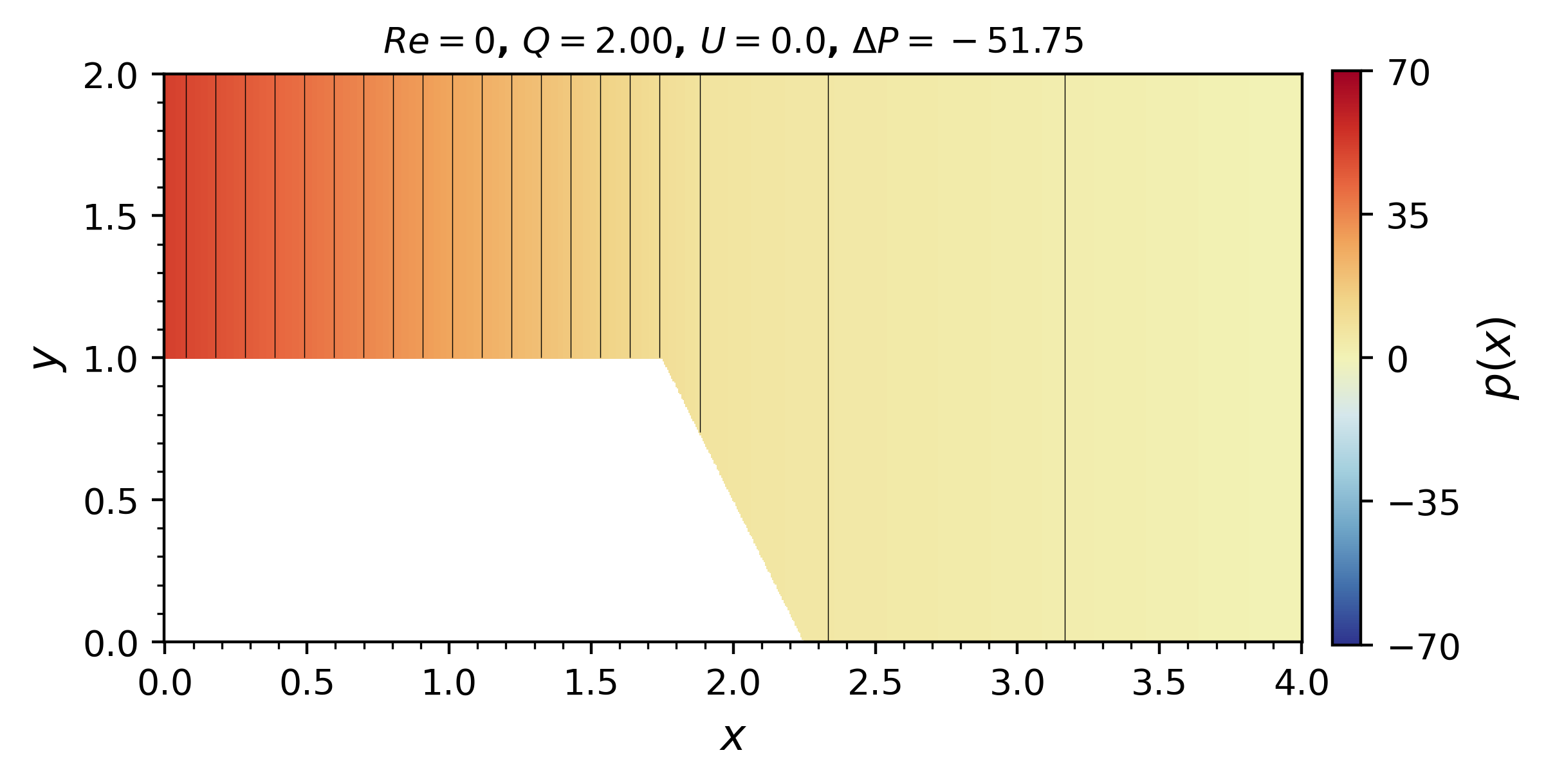
(d) Reynolds $\delta=0.25$

Figure 14: Pressure contours for the smoothed step bearing, $\mathcal{H}=2$. Contours from the Stokes solutions show significant pressure variation at the point of expansion in the film height.

The fluid resistance $\mathcal{R}$ for the Reynolds and Stokes solutions to the smoothed step bearing examples are shown in Fig. 15a as a function of $\delta$. The corresponding percent errors in resistance are shown in Fig. 15b. In the pipe flow limit of maximum $\delta$, the Reynolds and Stokes solutions have minimal error in resistance. Percent error in resistance increases as $\delta\to 0^{+}$, and the step geometry exhibits the largest error between the models.

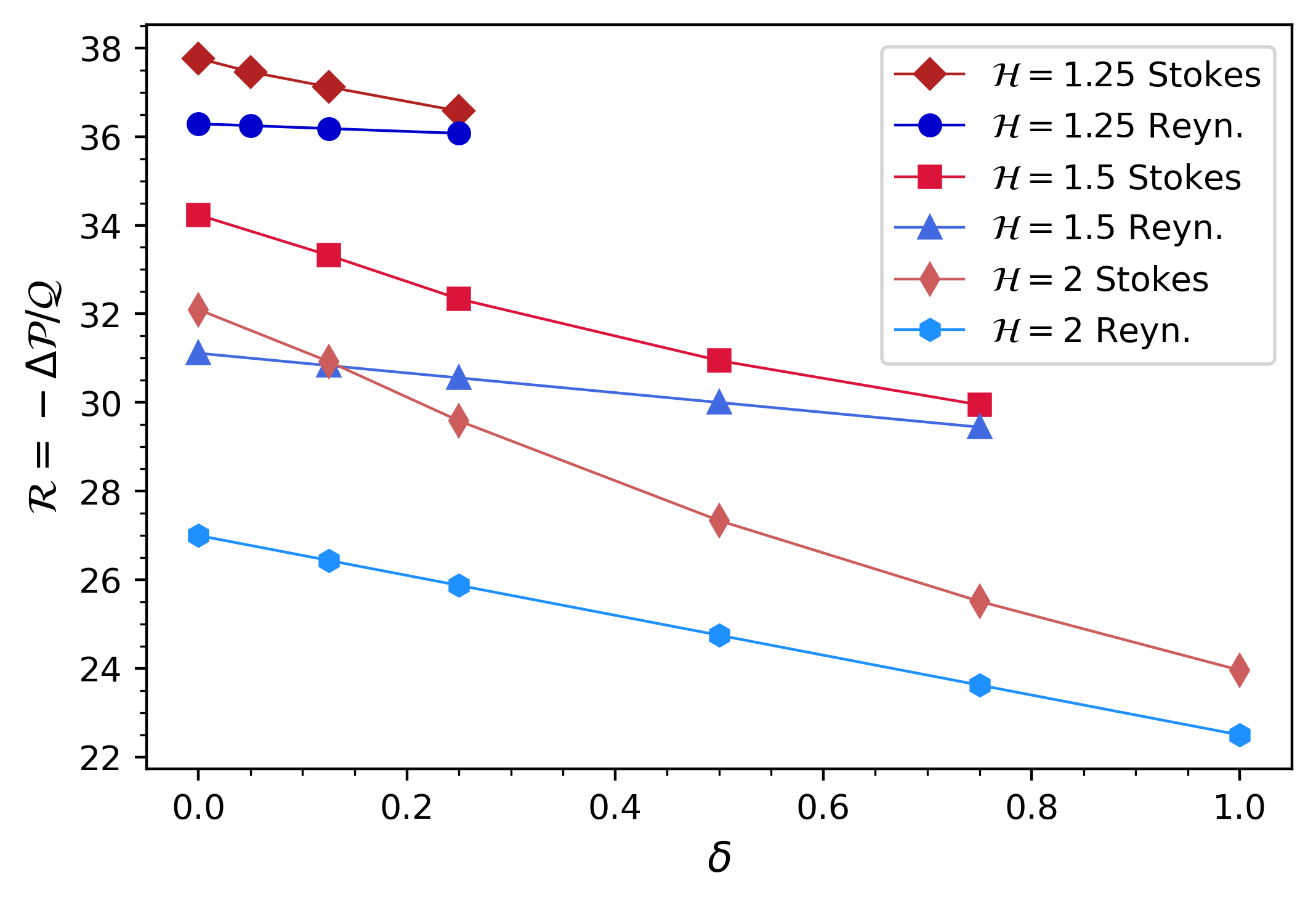
(a) Resistance

(b) $\%$-error in resistance

Figure 15: Resistance $\mathcal{R}$ for the smoothed step bearing, Stokes and Reynolds solutions. The step texturing limit $\delta\to 0^{+}$ has maximal percent error between the models.

5 Conclusions

Various examples of step bearings were observed with the Reynolds and Stokes equations. We considered two methods of solution to the Reynolds equation, Section 2. For textured bearings which are piecewise-linear by nature, an analytic solution is available in addition to the more general numerical finite difference method. The Stokes equations were solved using an iterative finite difference method for the biharmonic stream-velocity formulation, Section 3. The discrepancies observed between solutions to the Reynolds and Stokes equations characterize the extent to which the lubrication assumptions are applicable for each geometry.

In the BFS example, Section 4.1, increasing the expansion ratio increased the error in the resistance between the Reynolds and Stokes solutions. The sudden expansion at the step induced non-negligible cross-film pressure gradients not preserved in the lubrication approximation. Hence the pressure drop from the Stokes solutions is more extreme, likewise the resistance is higher than from the Reynolds solutions. Moreover, the region of corner flow recirculation in the BFS increases with increasing expansion ratio. Flow separation may be regarded as a response to significant pressure gradients upstream, and hence this phenomena is not observed in the lubrication approximation.

We then considered the Stokes solutions to the wedged corner variation of the BFS, Section 4.2. The $90^{\circ}$ angle downstream of the step was replaced by a triangular wedge. The bulk flow structure and channel resistance from the Stokes solutions were consistent with and without the wedge. Furthermore, the flow separation and reattachment points remained stable as the wedge was retracted and in the BFS limit. At low Reynolds numbers, regions of corner flow recirculation are very slow relative to the bulk flow; it may be desirable in applications to minimize such regions where fluid is stagnant.

Finally in the smoothed step bearing example, Section 4.3, we observed the effects of the expansion ratio and the slope of expansion on error between the Stokes and Reynolds solutions. The resistance decreased with increasing expansion ratio; the error in resistance increased with increasing expansion ratio. This is consistent with observations of the BFS. Furthermore, the error in resistance between the Reynolds and Stokes solutions increased with increasing slope of expansion. The models showed good agreement in the pipe flow limit, while step texturing exhibited maximal error for all expansion ratios.

In the analytic solution to the Reynolds equation, Section 2.2.2, we used the assumption that the pressure was continuous at the transition between piecewise-linear regions of the fluid film. Now having compared to the Stokes solutions, we see this assumption is a primary contributor to inaccuracy in the Reynolds equation. In all of the Stokes solutions to the BFS, wedged corner BFS, and smoothed step bearing examples, the cross-film pressure gradient was significant at points of sudden expansion, and increased in magnitude with increasing expansion ratio. A consequence of this work is that for a one dimensional approximation of pressure as in the Reynolds equation, one should carefully scrutinize the assumption of continuous pressure, particularly near singularities in the film height.

In conclusion, we find that large gradients in the surface geometry contribute to error between the Reynolds and Stokes solutions. Moreover, the solutions to the Reynolds equation do not capture corner flow recirculation. In future work, the performance of the lubrication assumptions may be evaluated for various other textured bearings; angular surface texturings in particular induce interesting patterns of flow recirculation according to the theory of Moffatt [13]. Furthermore, it is not well understood how the lubrication assumptions perform for a sequence of texturings, particularly when we consider that successive textures share the length scale. It may be that the geometry is long and thin, yet local surface discontinuities are not accurately modeled under the lubrication assumptions, and thus contribute to significant errors in the lubrication model.

Appendix A Convergence

A.1 The Reynolds finite difference and analytic solutions

The convergence of the Reynolds equation finite difference solution to the piecewise-linear analytic solution is shown in Fig. 16. Convergence for the BFS example with $\mathcal{H}=2$ is shown in Fig. 16a, and convergence for the smoothed step example with $\delta=0.25$, $\mathcal{H}=2$ is shown in Fig. 16b. The schematics of these examples are shown in Fig. 1 and Fig. 11 respectively. In the case of a continuous film height, like the smoothed step example, the error in $L_{\infty}$ norm converges at $\mathcal{O}(\Delta x^{2})$ as expected. In examples with a discontinuous height, like the BFS, the error in $L_{\infty}$ norm converges at $\mathcal{O}(\Delta x)$. This is not surprising: a finite difference approximation of a discontinuous height $h(x)$ will incur an error, while the piecewise-linear analytic method does not attempt to approximate $\frac{dh}{dx}$ near the discontinuity, and instead evaluates conditions on continuity of pressure and flux.

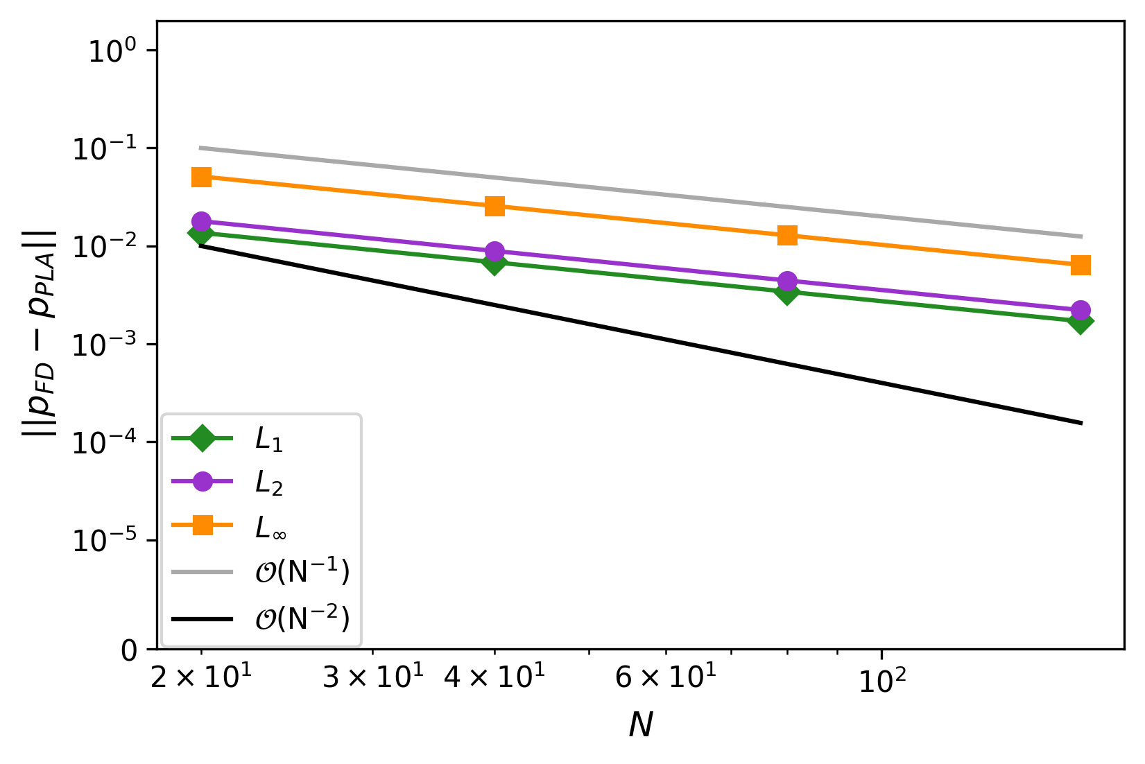
(a) BFS

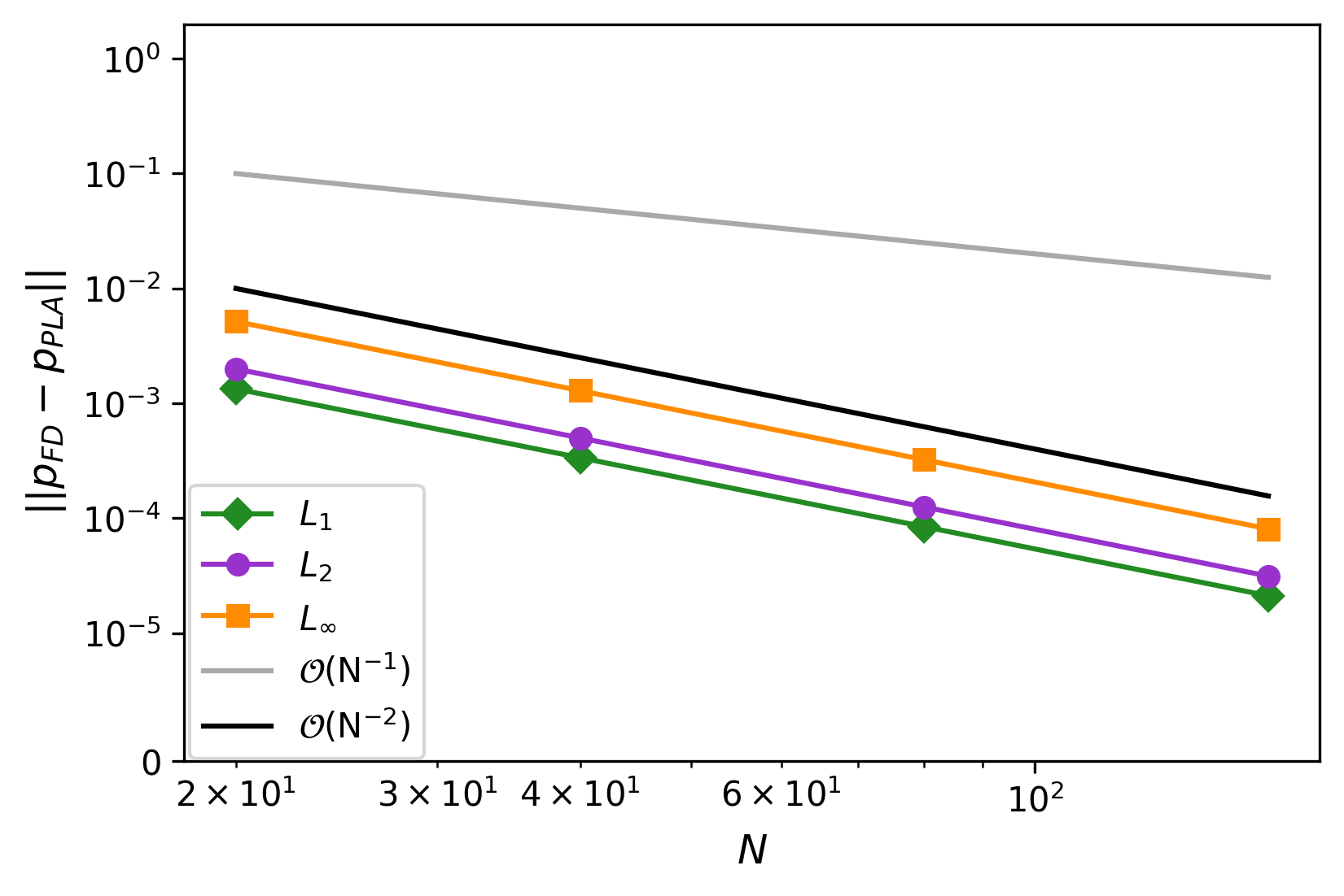
(b) Smoothed step bearing

Figure 16: Convergence of the pressure $p(x)$ from the Reynolds finite difference solution to the piecewise-linear analytic solution. For continuous film heights $h(x)$, convergence in is $\mathcal{O}(\Delta x^{2})$ in $L_{\infty}$ norm; otherwise, convergence is $\mathcal{O}(\Delta x)$ in $L_{\infty}$ norm.

A.2 The Stokes iterative finite difference solution

In the absence of an analytic solution to the Stokes equations, the convergence of the numerical solution is approximated by comparing to the solution with the finest available grid spacing ($\mathcal{N}=1/\Delta x=1/\Delta y$). Convergence plots for the stream function $\psi$ are shown in Fig. 17. Error is measured relative to $\mathcal{N}=320$, in $L_{1}$, $L_{2}$, and $L_{\infty}$ norms.

The convergence for the BFS example with $\mathcal{H}=2$ is shown in Fig. 17a, and convergence for the smoothed step example with $\delta=0.25$, $\mathcal{H}=1.5$ is shown in Fig. 17b. The schematics of these examples are shown in Fig. 1 and Fig. 11 respectively. For boundaries which are normal to the grid, like the BFS, convergence is $\mathcal{O}(\Delta x^{2})$ in $L_{\infty}$ norm. For boundaries which are non-rectilinear, like the smoothed step bearing, convergence is between $\mathcal{O}(\Delta x)$ and $\mathcal{O}(\Delta x^{2})$ in $L_{\infty}$ norm.

To increase this order of accuracy, it may be necessary to include more grid points in the interpolation Eq. 52. Equation Eq. 50 is accurate in the location of the boundary, however equation Eq. 52 might be updated based on five known values and not three. The limitation is that for grid points in acute corners, there may not be five points from the standard nine point stencil that fall interior to the domain.

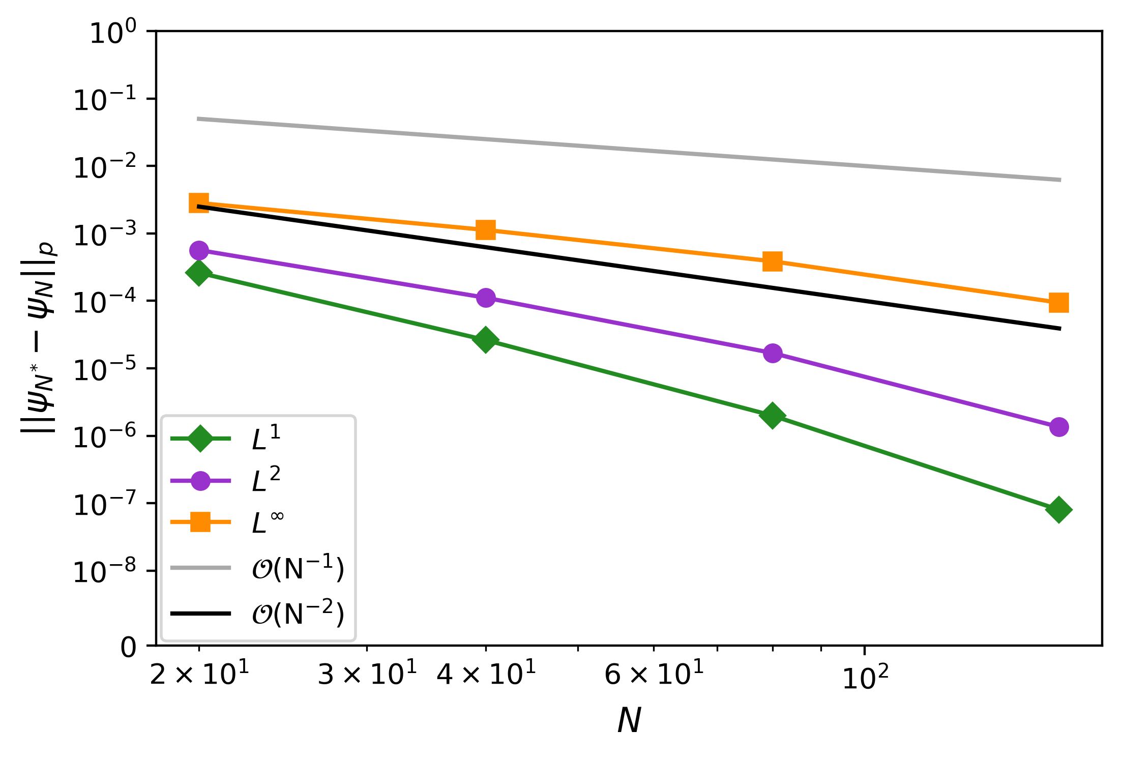
(a) BFS

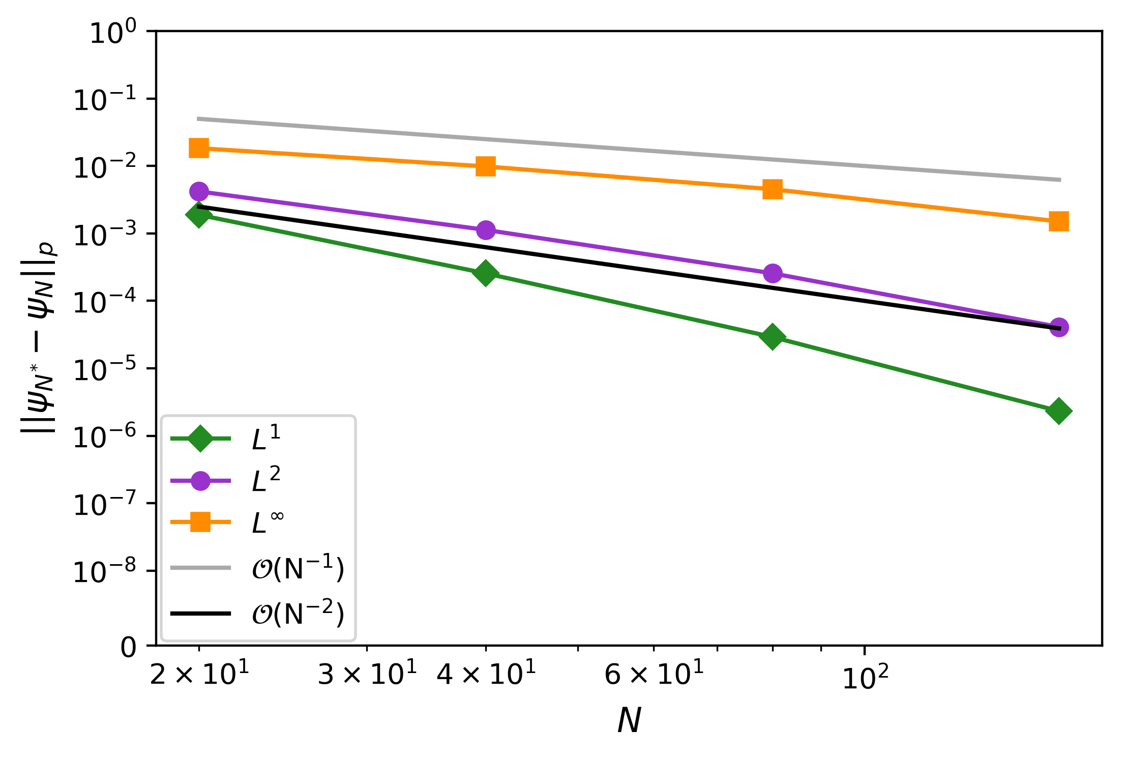
(b) Smoothed step bearing

Figure 17: Convergence of the stream function $\psi(x,y)$ from iterative Stokes finite difference solution. For examples with a grid aligned boundary, convergence is $\mathcal{O}(\Delta x^{2})$ in $L_{\infty}$ norm. Otherwise, convergence is between $\mathcal{O}(\Delta x)$ and $\mathcal{O}(\Delta x^{2})$ in $L_{\infty}$ norm.

References

- [1] M. Arghir, N. Roucou, M. Hélène, and J. Frene, Theoretical Analysis of the Incompressible Laminar Flow in a Macro-Roughness Cell, Journal of Tribology-Transactions of The Asme, 125 (2003), pp. 309–318, https://doi.org/10.1115/1.1506328.
- [2] B. F. Armaly, F. Durst, J. C. F. Pereira, and B. Schönung, Experimental and theoretical investigation of backward-facing step flow, Journal of Fluid Mechanics, 127 (1983), p. 473, https://doi.org/10.1017/S0022112083002839.
- [3] G. Biswas, M. Breuer, and F. Durst, Backward-Facing Step Flows for Various Expansion Ratios at Low and Moderate Reynolds Numbers, Journal of Fluids Engineering-Transactions of the Asme, 126 (2004), pp. 362–374, https://doi.org/10.1115/1.1760532.
- [4] S. Biswas and J. Kalita, HOC simulation of Moffatt eddies and its flow topology in the triangular cavity flow, Oct. 2017.
- [5] R. S. Brown, H. W. Stockman, and S. J. Reeves, Applicability of the Reynolds equation for modeling fluid flow between rough surfaces, Geophysical Research Letters, 22 (1995), pp. 2537–2540, https://doi.org/10.1029/95GL02666.
- [6] W. R. Dean and P. E. Montagnon, On the steady motion of viscous liquid in a corner, Mathematical Proceedings of the Cambridge Philosophical Society, 45 (1949), pp. 389–394, https://doi.org/10.1017/S0305004100025019.
- [7] M. Dobrica and M. Fillon, About the validity of Reynolds equation and inertia effects in textured sliders of infinite width, ARCHIVE Proceedings of the Institution of Mechanical Engineers Part J Journal of Engineering Tribology 1994-1996 (vols 208-210), 223 (2009), pp. 69–78, https://doi.org/10.1243/13506501JET433.
- [8] Y. Feldman, Y. Kligerman, I. Etsion, and S. Haber, The Validity of the Reynolds Equation in Modeling Hydrostatic Effects in Gas Lubricated Textured Parallel Surfaces, Journal of Tribology, 128 (2006), pp. 345–350.
- [9] M. Gupta and J. Kalita, A new paradigm for solving Navier–Stokes equations: streamfunction–velocity formulation, Journal of Computational Physics, 207 (2005), pp. 52–68, https://doi.org/10.1016/j.jcp.2005.01.002.
- [10] J. Julian, R. Anggara, and F. Wahyuni, The Influence of Fillet Step on Backward-Facing Step Flow Characteristics, Infotekmesin, 14 (2023), pp. 318–326, https://doi.org/10.35970/infotekmesin.v14i2.1919.
- [11] F. Marner, P. Gaskell, and M. Scholle, On a potential-velocity formulation of Navier-Stokes equations, Physical Mesomechanics, 17 (2014), pp. 124–130, https://doi.org/10.1134/S1029959914040110.
- [12] T. Matsui, M. Hiramatsu, and M. Hanaki, Separation of Low Reynolds Number Flows Around a Corner, Symposia on Turbulence in Liquids, 30 (1975), pp. 283–288.
- [13] H. K. Moffatt, Viscous and resistive eddies near a sharp corner, Journal of Fluid Mechanics, 18 (1964), pp. 1–18, https://doi.org/10.1017/S0022112064000015.
- [14] R. Rahmani, I. Mirzaee, A. Shirvani, and H. Shirvani, An analytical approach for analysis and optimisation of slider bearings with infinite width parallel textures, Tribology International, 43 (2010), pp. 1551–1565, https://doi.org/10.1016/j.triboint.2010.02.016.
- [15] S. Sen and J. C. Kalita, A 4OEC scheme for the biharmonic steady Navier–Stokes equations in non-rectangular domains, Computer Physics Communications, 196 (2015), pp. 113–133, https://doi.org/10.1016/j.cpc.2015.05.024.
- [16] F. Shen, C.-J. Yan, J.-F. Dai, and Z.-M. Liu, Recirculation Flow and Pressure Distributions in a Rayleigh Step Bearing, Advances in Tribology, 2018 (2018), pp. 1–8, https://doi.org/10.1155/2018/9480636.
- [17] S.-H. Shyu and W.-C. Hsu, A numerical study on the negligibility of cross-film pressure variation in infinitely wide plane slider bearing, Rayleigh step bearing and micro-grooved parallel slider bearing, Mechanical Sciences, 137 (2018), pp. 315–323, https://doi.org/10.1016/j.ijmecsci.2018.01.031.
- [18] Z. F. Tian and P. X. Yu, An efficient compact difference scheme for solving the streamfunction formulation of the incompressible Navier–Stokes equations, Journal of Computational Physics, 230 (2011), pp. 6404–6419, https://doi.org/10.1016/j.jcp.2010.12.031.
- [19] S. Uchida and M. Endo, On Some Numerical Solutions of the Flow Through a Back-Step channel., Memoirs of the Faculty of Engineering, Nagoya University, 21 (1975), pp. 152–161.