QNN-QRL: Quantum Neural Network Integrated with Quantum Reinforcement Learning for Quantum Key Distribution

Abstract

Quantum key distribution (QKD) has emerged as a critical component of secure communication in the quantum era, ensuring information-theoretic security. Despite its potential, there are issues in optimizing key generation rates, enhancing security, and incorporating QKD into practical implementations. This research introduces a unique framework for incorporating quantum machine learning (QML) algorithms, notably quantum reinforcement learning (QRL) and quantum neural networks (QNN), into QKD protocols to improve key generation performance. Here, we present two novel QRL-based algorithms, QRL-V.1 and QRL-V.2, and propose the standard BB84 and B92 protocols by integrating QNN algorithms to form QNN-BB84 and QNN-B92. Furthermore, we combine QNN with the above QRL-based algorithms to produce QNN-QRL-V.1 and QNN-QRL-V.2. These unique algorithms and established protocols are compared using evaluation metrics such as accuracy, precision, recall, F1 score, confusion matrices, and ROC curves. The results from the QNN-based proposed algorithms show considerable improvements in key generation quality. The existing and proposed models are investigated in the presence of different noisy channels to check their robustness. The proposed integration of QML algorithms into QKD protocols and their noisy analysis create a new paradigm for efficient key generation, which advances the practical implementation of QKD systems.

I Introduction

Quantum key distribution (QKD) is a promising technology to realize secure networks in quantum communication [1]. It has been used in the application of IoT-enabled medical devices to decrease power consumption [2]. Device-independent quantum key distribution (DI-QKD) offers the ultimate standard for secure key exchange that mitigates many quantum hacking risks that threaten non-DI QKD systems [3]. This systematically investigates security loopholes in commercial QKD devices, offering insights into current weaknesses and initiatives to strengthen secure key exchange over insecure channels [4]. This review discusses the use of QKD for secure key exchange, focusing on the BB84 protocol’s simulation, performance improvements, and its application potentials [5]. This survey presents the key challenges such as key rate, distance, cost, and practical security issues for commercial adoption of QKD and current solutions to them [6]. Quantum cryptography uses quantum mechanics for secure cryptographic tasks beyond QKD, such as quantum money [7], quantum cheque [8], randomness generations [9], and secure and delegated computations [10].

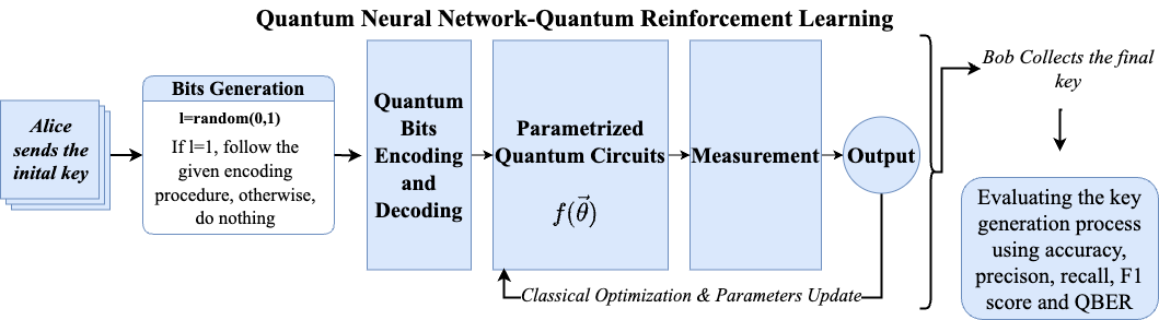
Figure 1: Schematic diagram showing the workings of the proposed QNN-QRL algorithm.

QKD faces numerous challenges, including limited key generation rates, restricted communication distances, practical implementation complexities, and security vulnerabilities arising from imperfect devices, all of which hinder its widespread adoption in quantum-safe communications [11]. Hacker attacks, the need for wireless implementations, and integration with existing telecommunications infrastructure add to these issues [12, 13]. Key protocols like BB84, B92, SARG04, and E91 have been developed to address these concerns by ensuring secure key transmission over long distances, maintaining high generation rates, and mitigating environmental and device deficiencies [14]. Despite the potential of one-time pad encoding for secure communication, global scalability remains a challenge, as demonstrated by advances in metropolitan, backbone optical fiber, and satellite-based free-space QKD networks [15]. Efforts to miniaturize continuous-variable systems for practical applications aim to overcome limitations in operational distance and key generation rates [16]. Rigorous metrology and robust classical authentication are crucial to mitigate vulnerabilities like side-channel attacks and ensure information-theoretic security over insecure channels [17, 18]. Current implementations often rely on computational security, necessitating integration with post-quantum cryptography for practical applications [19]. Addressing routing complexities, dependency on trusted nodes, and scalability issues are vital for extending secure QKD communication over longer distances [20]. Future research focuses on improving speed, range, and resilience while ensuring seamless integration into existing infrastructures and effective management of complexity and key consumption in real-world deployments [21].

Quantum machine learning (QML) approaches, such as quantum reinforcement learning (QRL) and quantum neural network (QNN) learning algorithms, offer promising solutions to the problem of QKD. QRL can improve resource allocation and routing protocols in QKD networks, enabling efficient key generation and secure communication over long distances while decreasing vulnerabilities associated with trusted relay nodes [22, 20]. QNNs can detect and prevent side-channel attacks and device faults by learning intricate patterns in noisy quantum signals and forecasting probable vulnerabilities [17, 21]. QRL-based frameworks may react dynamically to ambient conditions and device failures, improving scalability and robustness [19]. Integrating QNNs into authentication systems for conventional post-processing can improve resilience against denial-of-service attacks and reduce key consumption [18]. QML methods use quantum computing for real-time optimization and prediction, overcoming QKD’s limits in speed, scalability, and integration with existing networks [16]. These enhancements demonstrate QML’s transformative potential in overcoming QKD restrictions and paving the way for quantum-safe communication systems.

I-A Related Works

This work integrates machine learning (ML) with cascade error correction protocol that predicts the quantum bit error correction and final key length efficiently [23]. This uses deep learning models to detect and mitigate eavesdropping attacks [24]. They also use reinforcement learning (RL) to adaptively alter system settings in real-time to account for the noise profiles of different quantum channels. This introduces QKD networks enabled by software-defined networking (SDN) as a promising technology [25]. This explores the integration of IoT-enabled medical devices with QKD to enhance data security and energy efficiency in healthcare systems, particularly during pandemics like COVID-19 [2]. Three QKD protocols are demonstrated using IBM Q platforms [26]. This reviews recent developments, in-field deployments, and standardization advancements of QKD networks, highlighting their potential and challenges for large-scale commercialization [27]. This introduces the principles and requirements of QKD in practical scenarios and applications while highlighting advancements in its technical and architectural domains [28].

This shows that RL can efficiently allocate resources in QKD networks [29]. This study investigates QKD as a use case for QML, enhancing eavesdropping attacks on the BB84 protocol, developing a unique cloning mechanism for noisy environments, and building a collective attack utilizing QKD post-processing [30]. This study uses a Markov decision process and deep reinforcement learning (DRL) to optimize memory cutoff strategies for entanglement distribution over multi-segment repeater chains [31]. This proposes a DRL-based routing and resource assignment (RRA) scheme for QKD-secured optical networks (QKD-ONs), which outperforms traditional methods like deep Q-network (DQN), first-fit (FF), and random-fit (RF) across national science foundation network (NSFNET) and US backbone network (UBN24) [32]. This framework combines QKD, Multi-Objective Optimization (MOO), and RL to ensure safe and efficient data transmission in Smart Grid Advanced Metering Infrastructure (SGAMI) [33]. This demonstrates how RL optimizes resource allocation for efficient key distribution in QKD networks [34].

I-B Novelty and Contribution

Fig. 1 represents the schematic of the overall proposed quantum algorithms for the quantum key generation process. Though there are previous works on the key generation process, however, QML algorithms like QRL and QNN have not been integrated into them to investigate the quality of the key generation process. In this work, for the first time, QRL-based QKD protocols are proposed. Furthermore, QNN has been integrated into the existing BB84 and B92 protocols, along with the proposed QRL-based algorithms, to propose novel quantum algorithms for the quantum key generation process. They are named as QRL-V.1., QRL-V.2, QNN-BB84, QNN-B92, QNN-QRL-V.1, and QNN-QRL-V.2. Both the existing and proposed algorithms are run against six different noise channels to evaluate their performances. The following contributions are summarized point-wise.

• Two new QRL-based algorithms named, QRL-V.1, and QRL-V.2 are proposed for the quantum key generation process.

• QNN is integrated with the existing BB84, B92, and the proposed QRL-V.1. and QRL-V.2. algorithms to propose novel QNN-BB84, QNN-B92, QNN-QRL-V.1, and QNN-QRL-V.2 algorithms.

• A comparative analysis between the existing BB84, B92, and the above QRL-based and QNN-based algorithms is performed, and the results are evaluated in terms of evaluation metrics such as accuracy, precision, recall, and F1 score, confusion matrices and ROC curves.

• An extensive noise model analysis for the existing and proposed algorithms is made.

I-C Organization

The rest of the paper is organized as follows: Section II briefly discusses BB84, B92, QRL, and QNN algorithms. Section III presents the overall problem formulation and the proposed algorithms in detail. Then, in Section IV, the settings, datasets, preprocessing, hyperparameters, and overall results are presented. Finally, in Section V, the results are concluded.

II Background

II-A BB84 Protocol

The BB84 protocol, a cornerstone of QKD leverages the principles of quantum mechanics to securely share a cryptographic key between two parties, traditionally called Alice (sender) and Bob (receiver), even in the presence of an eavesdropper, Eve [35]. The BB84 protocol exploits two fundamental properties of quantum mechanics, such as superposition and measurement, and the no-cloning theorem: Alice selects a random sequence of bits, $b=\{b_{1},b_{2},\dots,b_{n}\}$, and a random sequence of bases, $r=\{r_{1},r_{2},\dots,r_{n}\}$, for encoding:

• Rectilinear basis ($+$): $\ket{0},\ket{1}$

• Diagonal basis ($\times$): $\ket{+}=\frac{1}{\sqrt{2}}(\ket{0}+\ket{1}),\;\ket{-}=\frac{1}{\sqrt{2}}(\ket{0}-\ket{1})$

For each bit $b_{i}$ and basis $r_{i}$:

• If $r_{i}=+$: encode $b_{i}=0$ as $\ket{0}$, $b_{i}=1$ as $\ket{1}$.

• If $r_{i}=\times$: encode $b_{i}=0$ as $\ket{+}$, $b_{i}=1$ as $\ket{-}$.

Alice transmits the encoded qubits through a quantum channel to Bob. Bob randomly selects bases $r^{\prime}=\{r^{\prime}_{1},r^{\prime}_{2},\dots,r^{\prime}_{n}\}$ to measure the incoming qubits:

• If $r^{\prime}_{i}=r_{i}$: Bob obtains the correct bit value $b_{i}$.

• If $r^{\prime}_{i}\neq r_{i}$: Bob’s measurement results are random.

Alice and Bob publicly announce their bases $r$ and $r^{\prime}$ (but not the bit values $b$) over a classical channel. They discard measurements where $r_{i}\neq r^{\prime}_{i}$. The rest of the bits shared between Alice and Bob form the sifted key. Alice and Bob reveal a subset of their sifted key to estimate the quantum bit error rate (QBER):

$$\text{QBER}=\frac{\text{Number of mismatched bits}}{\text{Total number of checked bits}}$$ (1)

If QBER exceeds a predefined threshold (e.g., $11\%$), they abort the protocol, suspecting eavesdropping. Alice and Bob apply error correction and privacy amplification to derive the final shared key. If Bob measures in the same basis as Alice:

$$P(\text{correct})=1$$ (2)

If Bob measures in a different basis:

$$P(\text{correct})=\frac{1}{2},\quad P(\text{incorrect})=\frac{1}{2}$$ (3)

If Eve intercepts and measures the qubits, she introduces errors due to the no-cloning theorem:

$$\text{Probability of introducing an error per qubit: }\frac{1}{4}.$$ (4)

II-B B92 Protocol

The B92 protocol, proposed by Bennett in 1992, is a simplified version of the BB84 QKD protocol [36]. Unlike BB84, which uses two orthogonal bases, the B92 protocol uses two non-orthogonal quantum states to encode a secret key. This simplification reduces the complexity of the protocol while retaining the security advantages of quantum mechanics. The B92 protocol leverages two primary quantum mechanical principles, such as non-orthogonal states and the no-cloning theorem: Alice chooses a random binary sequence $b=\{b_{1},b_{2},\dots,b_{n}\}$, where $b_{i}\in\{0,1\}$. She encodes these bits using two non-orthogonal states:

• $b_{i}=0$: $\ket{\psi_{0}}=\ket{0}$

• $b_{i}=1$: $\ket{\psi_{1}}=\ket{+}=\frac{1}{\sqrt{2}}(\ket{0}+\ket{1})$

These states are chosen such that:

$$\braket{\psi_{0}|\psi_{1}}=\frac{1}{\sqrt{2}},$$ (5)

indicating that they are not orthogonal. Alice sends the encoded quantum states $\ket{\psi_{i}}$ to Bob over a quantum channel, who randomly measures each received qubit in one of two bases:

• Rectilinear basis ($+$): $\{\ket{0},\ket{1}\}$

• Diagonal basis ($\times$): $\{\ket{+},\ket{-}\}$

If Bob’s measurement yields a conclusive result (i.e., $\ket{0}$ or $\ket{-}$), he assigns a corresponding bit value:

• Measurement outcome $\ket{0}$ corresponds to $b=0$.

• Measurement outcome $\ket{-}$ corresponds to $b=1$.

If Bob’s measurement is inconclusive, he discards the result. Bob communicates with Alice over a classical channel to confirm which measurements were conclusive. They discard bits corresponding to inconclusive measurements. Alice and Bob reveal a subset of their sifted key to estimate the QBER. If the QBER is within an acceptable range, they apply error correction and privacy amplification to generate the final secret key. In the B92 protocol, the overlap between the two non-orthogonal states determines the security of the protocol:

$$\braket{\psi_{0}|\psi_{1}}=\frac{1}{\sqrt{2}},$$ (6)

implying that the states cannot be perfectly distinguished. If Bob measures in the wrong basis, the probability of obtaining an inconclusive result is non-zero:

$$P(\text{inconclusive})=\left|\braket{\psi_{0}|\psi_{1}}\right|^{2}=\frac{1}{2}.$$ (7)

If Eve intercepts the qubits, she must guess the state, introducing errors with a probability proportional to the state overlap:

$$P(\text{error introduced})=1-\left|\braket{\psi_{0}|\psi_{1}}\right|^{2}=\frac{1}{2}.$$ (8)

II-C Quantum Reinforcement Learning

QRL integrates quantum computing with RL to enhance decision-making and optimize learning tasks in dynamic environments. In classical RL, agents interact with environments, performing actions $a_{t}$, observing states $s_{t}$, and receiving rewards $r_{t}$ to maximize cumulative returns $G_{t}$:

$$G_{t}=\sum_{k=0}^{\infty}\gamma^{k}r_{t+k},$$ (9)

where $\gamma$ is the discount factor. The optimal policy $\pi^{*}(s)$ maps states to actions, maximizing the expected return. QRL introduces quantum states $|\psi_{t}\rangle$, represented as:

$$|\psi_{t}\rangle=\sum_{i}c_{i}|i\rangle,$$ (10)

where $|i\rangle$ and $c_{i}$ are computational basis states and complex coefficients, respectively. Actions correspond to quantum operations, and rewards are encoded as quantum observables $\hat{R}$, with the goal of maximizing:

$$\langle\hat{R}\rangle=\langle\psi_{t}|\hat{R}|\psi_{t}\rangle.$$ (11)

The quantum value function $V(s)$, encoding the expected cumulative reward, can be optimized using quantum algorithms, while the quantum Bellman equation relates value functions to expected rewards:

$$V(s_{t})=\mathbb{E}\left[r_{t}+\gamma\langle\psi_{t+1}|\hat{H}|\psi_{t+1}\rangle\right],$$ (12)

where $\hat{H}$ is the system’s Hamiltonian at time $t+1$.

II-D Quantum Neural Network Algorithm

QNNs integrate quantum computing and machine learning, utilizing quantum mechanics to enhance neural network architectures. They leverage quantum properties such as superposition, entanglement, and interference to address problems infeasible for classical networks. This section outlines their structure, mathematical foundation, and advantages. QNNs consist of quantum gates and circuits, similar to layers in classical neural networks. Input data $x$ is encoded into a quantum state $|x\rangle$ via an embedding circuit, processed through parameterized quantum gates, and measured to generate predictions. The core operation is the parameterized quantum circuit $U(x,\theta)$, expressed mathematically as:

$$|\psi_{\text{output}}\rangle=U(x,\theta)|x\rangle,$$ (13)

where $|\psi_{\text{output}}\rangle$ is the quantum state post-processing. QNNs employ rotation gates and entangling gates. Single-qubit rotation gates are:

$$R_{x}(\theta)=e^{-i\frac{\theta}{2}X},R_{y}(\theta)=e^{-i\frac{\theta}{2}Y},R_{z}(\theta)=e^{-i\frac{\theta}{2}Z},$$ (14)

with $X,Y,Z$ being Pauli matrices and $\theta$ the rotation angle. Entangling gates like the controlled-NOT (CNOT) gate create quantum correlations:

$$\text{CNOT}=|0\rangle\langle 0|\otimes I+|1\rangle\langle 1|\otimes X.$$ (15)

II-E Training a QNN

Training involves iteratively optimizing parameters $\theta$ to minimize a loss function:

1. Encode input $x$ into $|x\rangle$.

2. Process $U(x,\theta)$ to compute the quantum state.

3. Measure the state for predictions $y_{\text{predicted}}$.

4. Compute the loss function:

   $$L(\theta)=\frac{1}{N}\sum_{i=1}^{N}\left(y_{\text{predicted},i}-y_{\text{true},i}\right)^{2},$$ (16)

   where $N$ is the number of samples.

5. Update $\theta$ using gradient descent:

   $$\theta\leftarrow\theta-\eta\nabla_{\theta}L(\theta),$$ (17)

   with $\eta$ as the learning rate.

QNNs offer unique benefits:

• Exponential Hilbert Space: Efficiently process high-dimensional data.

• Quantum Parallelism: Evaluate multiple states simultaneously.

• Entanglement: Model complex feature correlations.

QNNs merge quantum computation with neural network design, creating a powerful tool for optimization, data science, and AI. With advancing quantum hardware, they hold the potential to solve challenging problems across various domains.

III Methodology

III-A Problem Overview

The objective is to develop a QRL-based QKD algorithm, integrate the QNN model into the existing and QRL-based algorithms, and propose novel algorithms that can outperform the existing algorithms for the QKD process. A key is generated between two parties, Alice and Bob, where they follow different strategies to achieve this task. Here, a key is taken as $\{k_{1},k_{2},...,k_{n}\}$, which is generated by Alice, and sent to Bob over a channel. Bob then performs some measurements on those keys and forms a set of received keys $\{l_{1},l_{2},...l_{n}\}$. Accuracy, precision, recall, and F1 score are calculated from these two sets of keys. Furthermore, QBER is calculated, which is the amount of unmatching bits. The goal of the algorithm is to maximize the evaluation metrics, whereas to minimize the QBER.

$$\text{Evaluation metrics}=\text{max}\{\text{accuracy},\text{precision},\text{recall},\text{F1 score}\}$$ (18)

$$\text{Error rate}=\text{min}\{\text{QBER}\}$$ (19)

III-B QRL-V.1.

This proposed algorithm has the following steps:

• Alice randomly prepares 0 and 1, and encodes them using Hadamard and phase gate of arbitrary angle, $\theta_{1}$.

• Bob receives the encoded qubits and decodes them by using the QRL algorithm, where he determines the decoding angle $\theta_{2}$ from the algorithm, followed by another Hadamard operation.

• This requires no classical channel for making the final key. The algorithm learns the quantum circuit itself and decides the angle and chooses the closest value such that Alice’s bit can be predicted to finally prepare the key.

The following calculations from the quantum circuit (Fig. 3(a)) can be given as,

$$H\ket{0}=\frac{1}{\sqrt{2}}(\ket{0}+\ket{1})$$

$$\xrightarrow[P(-\theta_{2})]{P(\theta_{1})}\frac{1}{\sqrt{2}}(\ket{0}+e^{i\Delta\theta}\ket{1})$$

$$\xrightarrow[]{H}\frac{1+e^{i\Delta\theta}}{2}\ket{0}+\frac{1-e^{i\Delta\theta}}{2}\ket{1}$$ (20)

where, $\Delta\theta=\theta_{1}-\theta_{2}$, and $P0_{\ket{0}}$ and $P1_{\ket{0}}$ are the probabilities of 0 and 1, respectively after the measurement, and they can be calculated as follows,

$$P0_{\ket{0}}=\frac{1+\cos{\Delta\theta}}{2}=f1,\ P1_{\ket{0}}=\frac{1-\cos{\Delta\theta}}{2}=f2$$ (21)

The same calculation can be shown by taking the initial state as $\ket{1}$, and the probabilities of 0 and 1 ($P0_{\ket{1}}$ and $P1_{\ket{1}}$) are given as,

$$P0_{\ket{1}}=\frac{1-\cos{\Delta\theta}}{2}=f2,\ P1_{\ket{1}}=\frac{1+\cos{\Delta\theta}}{2}=f1$$ (22)

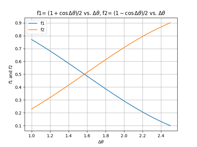
(a)

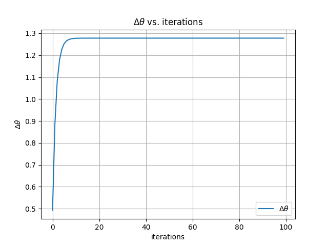
(b)

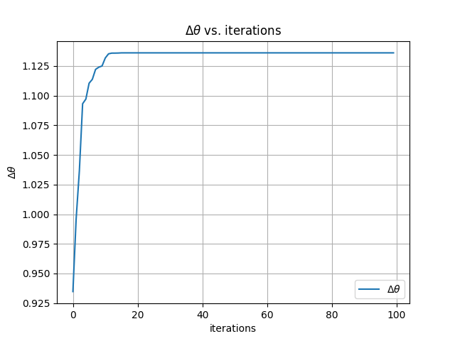
(c)

Figure 2: (a) Function plots versus angle. $\Delta\theta$ vs. number of iterations for (b) QRL-V.1., and (c) QRL-V.2.

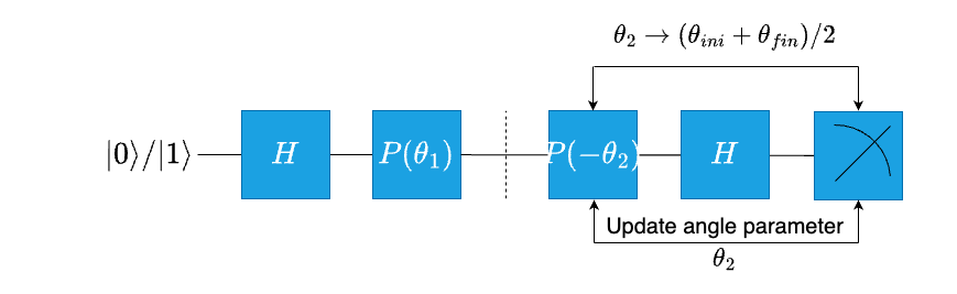
(a)

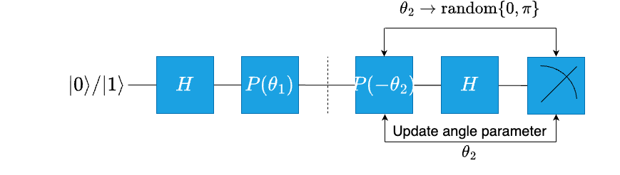
(b)

Figure 3: Quantum circuits representing (a) QRL-V.1 and (b) QRL-V.2 algorithms.

Input: Number of key bits $N$

Output: Final key $F_{k}$

1for $i=1$ to $N$ do

2    Sample a random bit $k_{i}\in\{0,1\}$

3    Sample a random angle $l_{i}\in[0,\pi]$

4   Initialize search intervals: $n_{1}^{i}=0$, $n_{2}^{i}=\pi/2$, $n_{3}^{i}=\pi$ for $j=1$ to $1000$ do

5       if $k_{i}=0$ then

6          Prepare qubit in $|0\rangle$ state

7      else

8          Prepare qubit in $|1\rangle$ state

9      

10      Apply Hadamard gate

11       Apply phase rotation gate with angle $l_{i}$

12      

13      Calculate midpoints: $m_{1}^{i}=(n_{1}^{i}+n_{2}^{i})/2$, $m_{2}^{i}=(n_{2}^{i}+n_{3}^{i})/2$

14      

15      Apply controlled-Z gate with phase $m_{1}^{i}$

16       Apply Hadamard gate

17      

18      Measure the qubit

19       Update search intervals based on measurement outcome and angle differences

20      

21   

22   Prepare qubit based on $k_{i}$

23    Apply Hadamard gate

24    Apply phase rotation gate with angle $l_{i}$

25    Apply controlled-Z gate with phase $(n_{1}^{i}+n_{3}^{i})/2$

26    Apply Hadamard gate

27    Measure the qubit

28    Add the measurement result to $K_{m}$

29   

Compare $K_{b}$ and $K_{m}$ to form the final key $F_{k}$

Algorithm 1 Quantum Key Generation: QRL-V.1.

Input: Number of key bits $N$

Output: Final key $F_{k}$

1for $i=1$ to $N$ do

2    Sample a random bit $k_{i}\in\{0,1\}$

3    Sample a random angle $l_{i}\in[0,\pi]$

4    Initialize search intervals: $n_{1}^{i}=0$, $n_{2}^{i}=\text{random}(0,\pi)$, $n_{3}^{i}=\pi$

5   

6   for $j=1$ to $100$ do

7       if $k_{i}=0$ then

8          Prepare qubit in $|0\rangle$ state

9      else

10          Prepare qubit in $|1\rangle$ state

11      

12      Apply Hadamard gate

13       Apply phase rotation gate with angle $l_{i}$

14      

15      Sample random midpoints: $m_{1}^{i}=\text{random}(0,n_{2}^{i})$, $m_{2}^{i}=n_{2}^{i}+\text{random}(0,n_{3}^{i}-n_{2}^{i})$

16      

17      Apply controlled-Z gate with phase $m_{1}^{i}$

18       Apply Hadamard gate

19      

20      Measure the qubit

21       Update search intervals based on measurement outcome and angle differences

22   

23   Prepare qubit based on $k_{i}$

24    Apply Hadamard gate

25    Apply phase rotation gate with angle $l_{i}$

26    Apply controlled-Z gate with phase $(n_{1}^{i}+n_{3}^{i})/2$

27    Apply Hadamard gate

28    Measure the qubit

29    Add the measurement result to $K_{m}$

Compare $K_{b}$ and $K_{m}$ to form the final key $F_{k}$

Algorithm 2 Quantum Key Generation: QRL-V.2.

(a)

(b)

Figure 4: Quantum circuits representing (a) QNN-BB84 and (b) QNN-B92 algorithms.

Input: Parameters $\theta$, Number of samples $S$, Number of key bits $N$

Output: Metrics: Accuracy, Precision, Recall, F1-Score, QBER

1

2for $s=1$ to $S$ do

3    Initialize empty lists: $K_{b}$, $K_{m}$, $F_{k}$

4   

5   for $i=1$ to $N$ do

6       Sample a random bit $k\in\{0,1\}$

7       if $k=1$ then

8          Prepare qubit in state $|1\rangle$ using $X$ gate

9      else

10          Prepare qubit in state $|0\rangle$

11      Append $k$ to $K_{b}$

12      

13      Sample a random basis $l\in\{0,1\}$

14       if $l=1$ then

15          Apply Hadamard gate to encode the basis

16      

17      Sample a random measurement basis $m\in\{0,1\}$

18       if $m=1$ then

19          Apply Hadamard gate to decode the basis

20      

21      Apply a customized parameterized circuit with $\theta$

22       Measure the qubit and retrieve result $p$

23       Append $p$ to $K_{m}$

24      

25      if $l=m$ then

26          Append $p$ to $F_{k}$

27      

28   

29   Compute metrics: Accuracy, Precision, Recall, F1-Score using $K_{b}$ and $K_{m}$

30    Compute QBER as $\text{QBER}=\frac{|F_{k}-K_{b}|}{|K_{b}|}$

31   

32Compute averages and standard deviations for all metrics

33 Print “QNN-BB84 Protocol” and metrics

Algorithm 3 Key Generation Process: QNN-BB84 Protocol

Input: Parameters $\theta$, Number of samples $S$, Number of key bits $N$

Output: Metrics: Accuracy, Precision, Recall, F1-Score, QBER

1

2for $s=1$ to $S$ do

3    Initialize empty lists: $K_{b}$, $K_{m}$, $F_{k}$

4   

5   for $i=1$ to $N$ do

6       Sample a random bit $k\in\{0,1\}$

7       if $k=1$ then

8          Prepare qubit in state $|+\rangle$ using Hadamard gate

9      else

10          Prepare qubit in state $|0\rangle$

11      Append $k$ to $K_{b}$

12      

13      Sample a random measurement basis $m\in\{0,1\}$

14       if $m=1$ then

15          Apply Hadamard gate to decode the basis

16      

17      Apply a customized parameterized circuit with $\theta$

18       Measure the qubit and retrieve result $p$

19       Append $p$ to $K_{m}$

20      

21      if $k=m$ then

22          Append $p$ to $F_{k}$

23      

24   

25   Compute metrics: Accuracy, Precision, Recall, F1-Score using $K_{b}$ and $K_{m}$

26    Compute QBER as $\text{QBER}=\frac{|F_{k}-K_{b}|}{|K_{b}|}\cdot 100$

27   

28Compute averages and standard deviations for all metrics

29 Print “QNN-B92 Protocol” and metrics

Algorithm 4 Key Generation Process: QNN-B92 Protocol

(a)

(b)

Figure 5: Quantum circuits representing (a) QNN-QRL-V.1 and (b) QNN-QRL-V.2 algorithms.

Input: Parameters $\theta$, Number of samples $S$, Number of key bits $N$, Number of iterations $I$

Output: Metrics: Accuracy, Precision, Recall, F1-Score, QBER

1

2for $s=1$ to $S$ do

3    Initialize empty lists: $K_{b}$, $K_{m}$, $F_{k}$

4   

5   for $i=1$ to $N$ do

6       Sample a random bit $k\in\{0,1\}$

7       Append $k$ to $K_{b}$

8      

9      Sample a random encoding phase $l\in[0,\pi]$

10      

11      Initialize decoding phases: $n_{1}=0$, $n_{2}=\pi/2$, $n_{3}=\pi$

12      

13      for $j=1$ to $I$ do

14          if $k=0$ then

15             Prepare qc0 as $|0\rangle$

16             Prepare qc1 as $|0\rangle$

17            

18         else

19             Prepare qc0 with $X$ gate applied to qubit $0$

20             Prepare qc1 with $X$ gate applied to qubit $0$

21            

22         

23         Apply Hadamard gate $H$, phase gate $P(l)$ to qc0 and qc1

24          Compute intermediate decoding phases $m_{1}=(n_{1}+n_{2})/2$, $m_{2}=(n_{2}+n_{3})/2$

25          Apply phase corrections $P(-m_{1})$ and $P(-m_{2})$

26          Apply customized parameterized circuit with $\theta$

27          Measure circuits qc0 and qc1

28         

29         Retrieve measurement results and compute probabilities $p_{0c0}$, $p_{0c1}$

30          Update decoding phase bounds $n_{1},n_{2},n_{3}$ based on $\Delta\theta_{1},\Delta\theta_{2}$

31         

32      

33      Compute final decoding phase $m=(n_{1}+n_{3})/2$

34       Prepare qc3 with corresponding $k$ state

35       Apply $H$, $P(l)$, and $P(-m)$ gates

36       Apply customized parameterized circuit with $\theta$

37       Measure qc3 and append result $p$ to $K_{m}$

38      

39   

40   Compare $K_{b}$ and $K_{m}$ to compute $F_{k}$

41    Compute metrics: Accuracy, Precision, Recall, F1-Score using $K_{b}$ and $K_{m}$

42    Compute QBER as $\text{QBER}=\frac{|F_{k}-K_{b}|}{|K_{b}|}\cdot 100$

43   

44

45Compute averages and standard deviations for all metrics

46 Print “QNN-QRL-V.1 Protocol” and metrics

Algorithm 5 Key Generation Process: QNN-QRL-V.1 Protocol

Input: Parameters $\theta$, Number of samples $S$, Number of key bits $N$, Number of iterations $I$

Output: Metrics: Accuracy, Precision, Recall, F1-Score, QBER

1

2for $s=1$ to $S$ do

3    Initialize empty lists: $K_{b}$, $K_{m}$, $F_{k}$

4   

5   for $i=1$ to $N$ do

6       Sample a random bit $k\in\{0,1\}$

7       Append $k$ to $K_{b}$

8      

9      Sample a random encoding phase $l\in[0,\pi]$

10      

11      Initialize decoding phases: $n_{1}=0$, $n_{2}\in[0,\pi]$, $n_{3}=\pi$

12      

13      for $j=1$ to $I$ do

14          if $k=0$ then

15             Prepare qc0 and qc1 in state $|0\rangle$

16            

17         else

18             Apply $X$ gate to qubit $0$ of qc0 and qc1

19            

20         

21         Apply $H$ gate and $P(l)$ gate to qc0 and qc1

22          Compute intermediate decoding phases:

23          $m_{1}=n_{1}+\texttt{rand}\cdot(n_{2}-n_{1})$,

24          $m_{2}=n_{2}+\texttt{rand}\cdot(n_{3}-n_{2})$

25          Apply $P(-m_{1})$ to qc0 and $P(-m_{2})$ to qc1

26          Apply $H$ gate to qc0 and qc1

27          Apply customized parameterized circuit with $\theta$

28          Measure qc0 and qc1

29         

30         Retrieve measurement results and compute probabilities $p_{0c0}$, $p_{0c1}$

31          Update decoding phase bounds $n_{1},n_{2},n_{3}$ based on $\Delta\theta_{1},\Delta\theta_{2}$

32         

33      

34      Compute final decoding phase $m=(n_{1}+n_{3})/2$

35       Prepare qc3 in state corresponding to $k$

36       Apply $H$, $P(l)$, and $P(-m)$ gates to qc3

37       Apply customized parameterized circuit with $\theta$

38       Measure qc3 and append the result $p$ to $K_{m}$

39      

40   

41   Compare $K_{b}$ and $K_{m}$ to compute $F_{k}$

42    Compute metrics: Accuracy, Precision, Recall, F1-Score using $K_{b}$ and $K_{m}$

43    Compute QBER as $\text{QBER}=\frac{|F_{k}-K_{b}|}{|K_{b}|}\cdot 100$

44   

45Compute averages and standard deviations for all metrics

46 Print “QNN-QRL-V.2 Protocol” and metrics

Algorithm 6 Quantum Key Generation Process: QNN-QRL-V.2 Protocol

Here are the following strategies followed for the quantum reinforcement learning algorithm. $P0_{\ket{0}}$, $P1_{\ket{0}}$, $P0_{\ket{1}}$, and $P1_{\ket{1}}$ are plotted against $\Delta\theta$, where it is found that when Alice sends 0, $P0_{\ket{0}}>P1_{\ket{0}}$ (let us say around the value of 1.2), and when Alice sends 1, $P0_{\ket{1}}<P1_{\ket{1}}$ around the same value. So, there is a clear distinction for extracting information about what Alice sends. The plots shown in Fig. 2(a) clearly represent the above strategy. So, two strategies are developed for choosing $\theta_{2}$ such that, $\Delta\theta$ converges around 1.2. In this case, two angles are chosen, one is the initial value of the range ($n1$), and the second value is the final value of the range ($n3$). In the first iteration of the algorithm, the angle value ($n2$) is the summation of $n1$ and $n2$ divided by 2. $n2$ creates two ranges, where the algorithm learns the function value such that in the next iteration, the range is decided, and accordingly, $n1$, $n2$, and $n3$ are updated. This process is repeated until $\Delta\theta$ reaches to 1.2. This strategy is explained in Algorithm 1. The quantum circuit of the overall algorithm is shown in Fig. 3(a). From the circuit, it can be observed that Alice prepares $\ket{0}/\ket{1}$, after which the application of Hadamard operations, followed by phase gates with an angle $\theta_{1}$. Bob then receives the qubit and applies angle $\theta_{2}$ in the reverse order, followed by Hadamard operations. Now, the QRL algorithm learns Bob’s angle parameter, such that, $\Delta\theta$ reaches a particular value, and the final bit is declared. From the graph 2(b), it is clear that, after a number of iterations, $\Delta\theta$ reaches a value around 1.2, where, $f1(\Delta\theta)$ is greater than $f2(\Delta\theta)$, which will help in deciding the bit sent by Alice.

III-C QRL-V.2.

In this procedure, the above same process is repeated, with the only difference being the selection of $\theta$ values. In this scenario, the next $\theta$ is picked randomly rather than dividing the entire range by 2, so that $\Delta\theta$ converges around 1.2. The initial two ranges are also determined by randomly selecting an angle from the original range. The functions are calculated in both ranges, and the next range is carried forward. A random angle value chosen and the process is repeated until $\Delta\theta$ hits 1.2. This is the only difference from the QRL-V.1 algorithm. QRL-V.2 is another version of QRL-V.1, thus we refer to it as such. Algorithm 2 provides a step-by-step process. Figure 3(b) depicts the quantum circuit for the entire algorithm. This technique uses the same quantum circuit as the previous QRL-V.1 algorithm; however, the learning strategy changes, involving the random selection of Bob’s angle parameter, which ultimately determines the final bit received by Bob. The graph 2(c) shows that using this technique, after a number of iterations, $\Delta\theta$ reaches a value around 1.2, where $f1(\Delta\theta)$ bigger than $f2(\Delta\theta)$, which will help in choosing the bit transmitted by Alice.

III-D QNN-BB84

This is an integrated method of QNN and BB84 protocol. Mainly, in the BB84 protocol, the QNN algorithm has been integrated to improve its efficiency. The schematic diagram representing the algorithm is depicted in Fig. 4(a). From the circuit, it is clear that Alice prepares $\ket{0}/\ket{1}$ states and randomly encodes them using Identity (I) or Hadamard (H) operations and sends them to Bob. After receiving the qubit, Bob randomly performs I or H operations. This completes the BB84 protocol, which follows for multiple number of sequences of bits. Now, the QNN algorithm is integrated, where a parametrized quantum circuit (PQC) is used, denoted by $\vec{\theta}$. This is the learning vector parameter in the quantum circuit that learns to maximize the accuracy of the overall algorithm, that is to collect the final key with the least QBER and the maximum matching with the initial key sent by Alice. The step-by-step process is given in Algorithm 3.

III-E QNN-B92

This approach combines QNN and the B92 protocol. Specifically, the QNN algorithm has been implemented into the B92 protocol to improve its efficiency. Fig. 4(b) shows a schematic illustration of the algorithm. The quantum circuit displays Alice preparing $\ket{0}/\ket{1}$ states and randomly encoding them using the Identity (I) operation before sending them to Bob. After obtaining the qubit, Bob randomly performs I or H operations. This completes the B92 protocol, which is used for a multiple number of bit sequences. The QNN method is integrated using a PQC represented by $\vec{\theta}$. This is the learning vector parameter in the quantum circuit that learns to maximize the overall algorithm’s accuracy, i.e., collect the final key with the lowest QBER and the closest match to Alice’s generated key. Algorithm 4 provides a step-by-step method.

III-F QNN-QRL-V.1.

This is an integrated method of QNN and QRL-V.1. protocol. Mainly, in the QRL-V.1 protocol, the QNN algorithm has been integrated to improve its efficiency. The schematic diagram representing the algorithm is depicted in Fig. 5(a). In this case, the initial part of the quantum circuit is the same as that of the QRL-V.1. At the end of the circuit, the PQC is added to integrate the QNN algorithm with this method. The learning angle vector $\vec{\theta}$ learns the whole algorithm to find the optimal parameter such that the angle parameter $\theta_{2}$ gets the appropriate value, along with maximizing the overall accuracy of the whole algorithm. It is worth noticing that the algorithm learns the $\theta_{2}$ parameter of Bob (which comes from the QRL algorithm) and angle vector $\vec{\theta}$ (that comes from the QNN algorithm), hence integrating both QRL-V.1 and QNN algorithms into one protocol, leading to the QNN-QRL-V.1 algorithm. The strategy of choosing $\theta_{2}$ follows the QRL-V.1 algorithm, and the strategy for finding $\vec{\theta}$ follows optimizing the objective function that maximizes the accuracy of the overall algorithm. The step-by-step process is given in Algorithm 5.

III-G QNN-QRL-V.2.

This is an integrated approach of QNN and QRL-V.2. protocol. Specifically, the QRL-V.2 protocol incorporates the QNN algorithm to boost its efficiency. Fig. 5(b) shows a schematic illustration of the algorithm. In this scenario, the quantum circuit’s initial component is identical to that of the QRL-V.2. The difference is that at the end of the circuit, a PQC is introduced to integrate the QNN algorithm into this technique. The learning angle vector $\vec{\theta}$ learns the whole algorithm to find the optimal parameter so that the angle parameter $\theta_{2}$ gets the appropriate value, while also maximizing the overall accuracy of the algorithm. The algorithm learns Bob’s $\theta_{2}$ parameter (from the QRL algorithm) and angle vector $\vec{\theta}$ (from the QNN algorithm), combining the QRL-V.2 and QNN algorithms into a single protocol, resulting in the QNN-QRL-V.2 algorithm. The approach for selecting $\theta_{2}$ is based on the QRL-V.2 algorithm, which randomly selects a value from a specific interval with each iteration. The strategy for determining $\vec{\theta}$ is based on maximizing the objective function to optimize the algorithm’s accuracy. Algorithm 6 provides a step-by-step process.

Protocols	Accuracy	Precision	Recall	F1 Score	QBER
BB84	0.720 $\pm$ 0.108	0.674 $\pm$ 0.157	0.790 $\pm$ 0.203	0.704 $\pm$ 0.118	0.580 $\pm$ 0.116
B92	0.530 $\pm$ 0.135	0.550 $\pm$ 0.275	0.361 $\pm$ 0.165	0.421 $\pm$ 0.185	0.480 $\pm$ 0.188
QRL-QKD-V.1	0.567 $\pm$ 0.196	0.541 $\pm$ 0.211	0.651 $\pm$ 0.245	0.568 $\pm$ 0.191	0.500 $\pm$ 0.161
QRL-QKD-V.2	0.542 $\pm$ 0.183	0.544 $\pm$ 0.209	0.576 $\pm$ 0.241	0.532 $\pm$ 0.177	0.580 $\pm$ 0.140
QNN-BB84	1.000 $\pm$ 0.000	1.000 $\pm$ 0.000	1.000 $\pm$ 0.000	1.000 $\pm$ 0.000	0.420 $\pm$ 0.117
QNN-B92	0.610 $\pm$ 0.094	0.573 $\pm$ 0.107	0.673 $\pm$ 0.231	0.588 $\pm$ 0.094	0.490 $\pm$ 0.144
QNN-QRL-V.1	1.000 $\pm$ 0.000	1.000 $\pm$ 0.000	1.000 $\pm$ 0.000	1.000 $\pm$ 0.000	0.000 $\pm$ 0.000
QNN-QRL-V.2	1.000 $\pm$ 0.000	1.000 $\pm$ 0.000	1.000 $\pm$ 0.000	1.000 $\pm$ 0.000	0.000 $\pm$ 0.000

TABLE I: Evaluation metrics for the existing and proposed algorithms

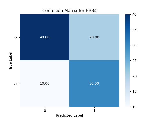
(a)

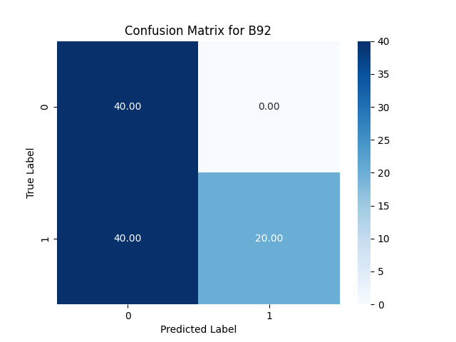
(b)

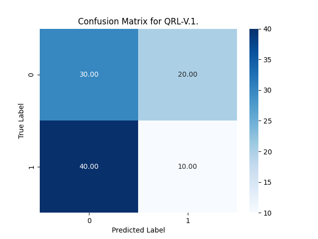
(c)

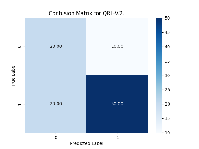
(d)

Figure 6: Confusion matrices for the algorithms BB84, B92, QRL-V.1., and QRL-V.2.

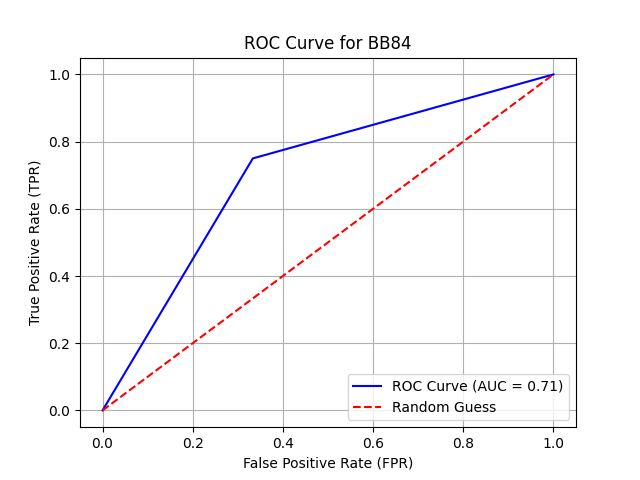
(a)

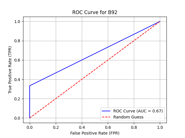
(b)

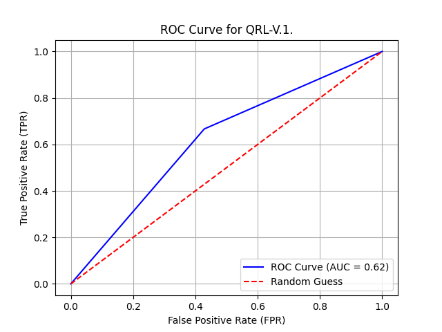
(c)

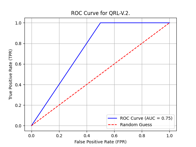
(d)

Figure 7: ROC curves for the algorithms BB84, B92, QRL-V.1., and QRL-V.2.

(a)

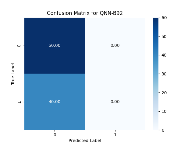
(b)

(c)

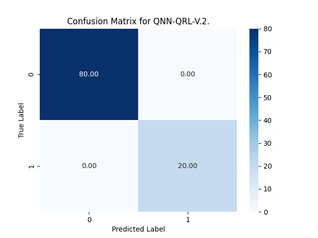
(d)

Figure 8: Confusion matrices for the QNN integrated algorithms BB84, B92, QRL-V.1., and QRL-V.2.

(a)

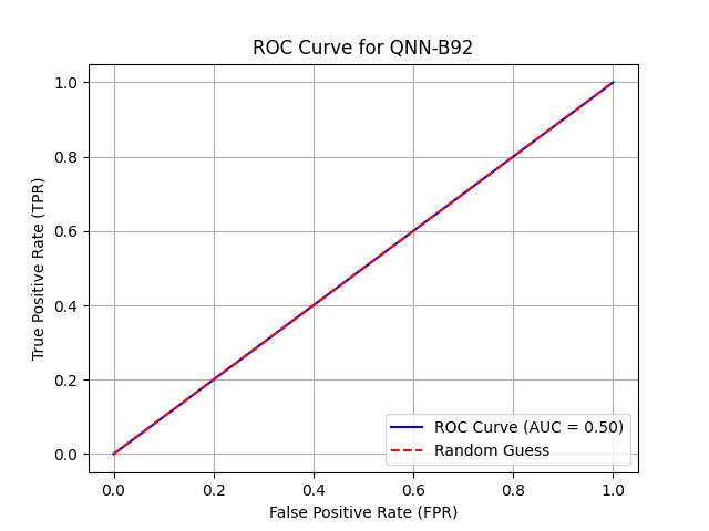
(b)

(c)

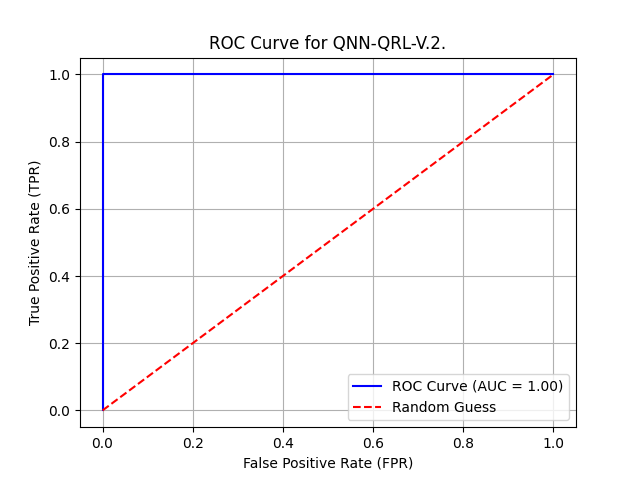
(d)

Figure 9: ROC curves for the QNN integrated algorithms BB84, B92, QRL-V.1., and QRL-V.2.

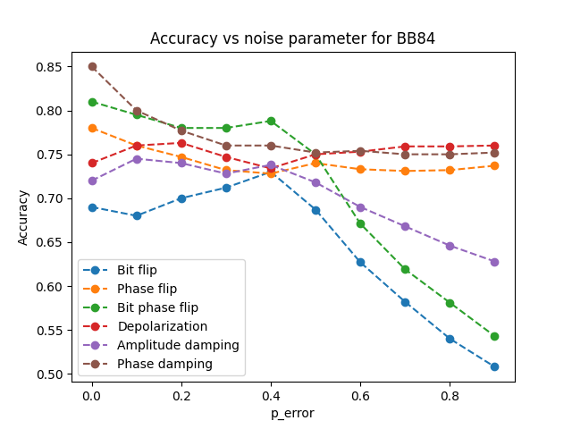
(a)

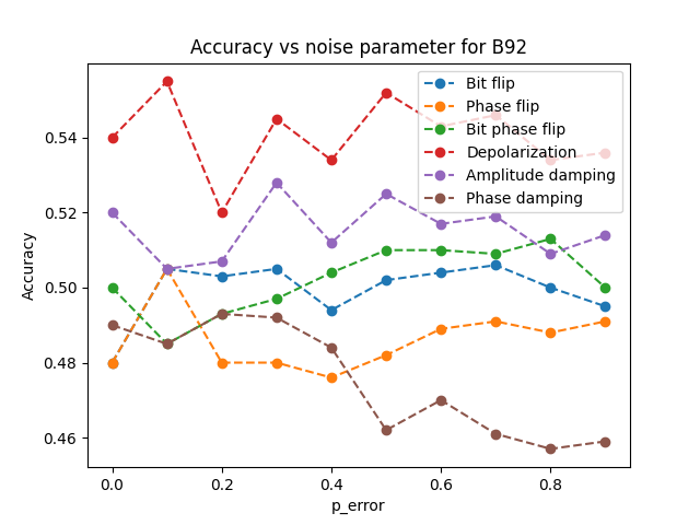
(b)

(c)

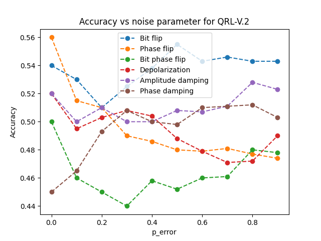
(d)

Figure 10: Noise plots for a) BB84, b) B92, c) QRL-V.1 and d) QRL-V.2.

(a)

(b)

(c)

(d)

Figure 11: Noise plots for a) QNN-BB84, b) QNN-B92, c) QNN-QRL-V.1 and d) QNN-QRL-V.2.

IV Experimental Results

IV-A Datasets, Preprocessing and Hyperparameters

The dataset mainly involves the key generation process which is performed using random generation of bits by Alice and sent to Bob for further processing. The algorithm supports the generation keys of length 100 to 1000-bit strings for collecting faster results. There are no preprocessing steps involved however, the key generation process uses a random value between 0 and 1, and accordingly decides the quantum operations for encoding and decoding in the quantum circuit involved in the respective protocols. The QISKit platform is used for the experiment, where an ‘automatic’ simulator is used with 1024 numbers of shots. For the optimization of the circuit parameters, a Cobyla optimizer is used. The number of iterations taken for QNN integrated algorithms is 5, however, in the first iteration itself, the best results are achieved.

IV-B Noise Models

Investigating various noise models, including bit flip, phase flip, bit-phase flip, depolarizing, amplitude damping, and phase damping, is crucial for understanding the robustness and dependability of quantum algorithms in real-world circumstances [37]. These noise models depict different types of quantum errors caused by interactions with the environment. For example, bit flip errors change the state of a qubit, whereas phase flip errors affect the phase of the quantum state. Depolarizing noise causes random mistakes, whereas amplitude damping simulates energy loss, a major problem with superconducting qubits. Phase damping describes the loss of quantum coherence without requiring energy dissipation.

IV-C Results

From Table I, it is observed that BB84 has achieved an accuracy of 0.720 $\pm$ 0.108, while B92 has achieved an accuracy of 0.530 $\pm$ 0.135. Hence, the accuracy of the BB84 protocol is higher than that of B92. Additionally, BB84’s other evaluation metrics also have higher values as compared to the B92 protocol. However, the BB84’s QBER value is 0.580 $\pm$ 0.116, which is higher than that of B92. Hence, even if the BB84’s accuracy and other evaluation metric values are higher, the QBER is also higher as compared to B92. The QRL-based algorithms such as QRL-QKD-V.1 and QRL-QKD-V.2 have performed similar accuracies compared to the B92 protocol. However, their precision, recall, and F1 score are better than the B92 protocol. The QBERs of QRL-based protocols are a little higher than that of B92. Both the QRL-based protocols have similar metric values. It can be noted that QNN-integrated algorithms show significant improvement over the traditional and QRL-based algorithms. QNN-BB84 has performed the best evaluation metrics values of 1.000 $\pm$ 0.000, for accuracy, precision, recall and F1 score, while it has the lower QBER value, i.e., 0.420 $\pm$ 0.117 as compared to BB84 protocol. Similarly, QNN-QRL-V.1 and QNN-QRL-V.2 have the best accuracy, precision, recall and F1 score of $1.000\pm 0.000$, while their QBER is $0.000\pm 0.000$ which is the lowest among all the algorithms. QNN-B92 has an accuracy of $0.610\pm 0.094$, which is higher than the B92 protocol, and its QBER is $0.490\pm 0.144$ which is near the value of B92.

The confusion matrices for the algorithms BB84, B92, QRL-V.1, and QRL-V.2 are given in Fig. 6. It can be observed that the amount of true classification is 70%, 60%, 40%, and 70% for the BB84, B92, QRL-V.1, and QRL-V.2 algorithms respectively. BB84 and QRL-V.2. are the best performers among them, while QRL-V.2 is the worst performer among them. This suggests the amount of misclassification of keys is the highest in the case of QRL-V.1 as compared to the other algorithms, leading to 60%. It can be noted that the amount of misclassification of one of the classes for B92 is completely zero. In Fig. 7, the ROC curves of the above algorithms are shown. The AUC scores of BB84, B92, QRL-V.1, and QRL-V.2 are 0.71, 0.67, 0.62, and 0.75. It can be noted that the AUC score of QRL-V.2 is the best among the above algorithms, which is followed by BB84, and B92, while QRL-V.1 has the lowest AUC score. This means the true positive rate in the case of QRL-V.2 is the highest leading to one of the most feasible and best methods among these algorithms. In other words, the QRL-V.2 has outperformed the other algorithm in terms of AUC score.

Fig. 8 illustrates the confusion matrices for all QNN integrated algorithms, including QNN-BB84, QNN-B92, QNN-QRL-V.1, and QNN-QRL-V.2. The QNN-BB84, QNN-B92, QNN-QRL-V.1, and QNN-QRL-V.2 algorithms achieve 100%, 60%, 100%, and 100% true classification, respectively. QNN-BB84, QNN-QRL-V.1, and QRL-V.2 outperform them all, with QNN-B92 placing the worst. QNN-B92 has the largest rate of key misclassification compared to other algorithms, resulting in 40%. It should be emphasized that the other algorithms generate no misclassification. Fig. 9 depicts the ROC curves for the above algorithms. The AUC values for QNN-BB84, QNN-B92, QNN-QRL-V.1, and QNN-QRL-V.2 are respectively 1.0, 0.5, 1.0, and 1.0. It is worth noting that QNN-BB84, QNN-QRL-V.1, and QNN-QRL-V.2 have the highest AUC scores among the algorithms mentioned above, while QNN-B92 has the lowest. This suggests that QNN-BB84, QNN-QRL-V.1, and QNN-QRL-V.2 have the highest true positive rates, making them one of the most viable and effective approaches among all proposed and current algorithms.

IV-D Noisy Results

From Fig. 10(a), it can be observed that the accuracy performance is greatly impacted by the bit-flip noise model, where the accuracy has dropped from 0.7 to 0.5. It is interesting to note that, around the noise parameter of near 0.4 value, the accuracy increases to a height of near 0.75. Then, next, it is impacted by the bitphaseflip noise model, where the accuracy drops from 0.8 to 0.55 showing a similar peak around near 0.4 noise parameter value. Next, amplitude damping noise affects the most, whereas the rest of the models fluctuate in a similar range throughout noise parameters. Hence, the BB84 protocol shows robustness against the other rest noise models. From Fig. 10(b), it can be observed that there is no significant decrease in the accuracy of the B92 protocol for all noise models. So in a sense, it can be said that the B92 protocol is the most effective against all noise models. It can be mentioned that some of the noise models show an increase in accuracy with an increase in noise parameters, specifically bit flip, phase flip, and bit phase flip, showing a consistent increase in accuracy with an increase in noise parameters, while some others show some increment in accuracy then dropping the accuracy, such as depolarizing, amplitude damping, and phase damping. From Fig. 10(c), it can be observed that for noise models such as bit flip, phase flip, bit phase flip, and amplitude damping, the accuracy fluctuates between 0.5 and 0.56. On the other hand, for depolarizing and phase damping, the accuracy fluctuates between 0.44 and 0.5. It is worth noting that both the depolarizing and phase-damping accuracies are increasing with the increase of noise parameters. From Fig. 10(d), it can be observed that all the noise models vary between 0.44 and 0.56. In the phase flip and phase damping noise models, the accuracies are steadily decreasing and increasing, respectively.

In Fig. 11, the accuracies for QNN integrated models against different noisy channels are presented. From Fig. 11(a), it is observed that the accuracy of QNN-BB84 against phase flip, depolarizing, and phase damping noise remains almost constant and not greatly impacted by the noise parameters. Whereas, the accuracies for bit flip, bit phase flip, and amplitude damping are greatly impacted by the noise parameters reaching around 0.55 for bit flip and bit phase flip, whereas the accuracy for amplitude damping is reaching near 0.7. From Fig. 11(b), it is clear that all the noise models’ accuracies are saturating around 0.5 irrespective of their starting points. It is worth noting that phase damping and depolarizing accuracies are increasing from the starting point, whereas the rest are decreasing till they saturate. From Fig. 11(c), it can be seen that the phase flip, depolarizing, and phase damping accuracies stay constant throughout the noise parameter range, while bit flip, bit phase flip, and amplitude damping are declining after a certain noise parameter. For example, bit flip and bit phase flip accuracies decline after 0.4 noise parameters and reach 0.5 accuracy, whereas the accuracy for amplitude damping declines after 0.2 noise parameters and reaches around 0.7. In Fig. 11(d), the phase flip, bit phase flip, and depolarizing behave similarly to the previous one, while the bit flip, bit phase flip, and amplitude damping have a little different behaviour. The bit flip and bit phase flip accuracies decline after 0.4 and reach 0 accuracy after 0.6 noise parameter. The amplitude damping accuracy declines after 0.2 and then after 0.4, again increasing the accuracy to 0.4 at the maximum noise.

IV-E Discussion

The reported results demonstrate the comparative performance of classical QKD protocols, QRL-based algorithms, and QNN-integrated protocols in terms of the quantum key generation process. The investigation shows that classical protocols, such as BB84, outperform B92 in accuracy and evaluation measures, but have higher QBER values, indicating a trade-off between performance metrics and error rates. BB84 achieves a commendable balance, with an AUC score of 0.71, proving its viability in actual applications. However, the QBER ($0.580\pm 0.116)$ indicates potential for improvement in terms of error minimization. QRL-based protocols, specifically QRL-QKD-V.1 and QRL-QKD-V.2, achieve equivalent accuracy to B92 while outperforming it in precision, recall, and F1 scores, demonstrating its efficiency in increasing classification quality. Notably, QRL-V.2 has the highest AUC score (0.75) among non-QNN algorithms, showing higher true positive rates and highlighting its potential as a viable alternative to classic QKD procedures. However, the somewhat higher QBER values for QRL-based protocols indicate that additional optimization is required to reduce errors in key generation.

The QNN-integrated algorithms indicate a significant boost in performance, outperforming all evaluation metrics. QNN-BB84, QNN-QRL-V.1, and QNN-QRL-V.2 achieve flawless accuracy ($1.000\pm 0.000$), precision, recall, and F1 scores, and have the lowest QBER values among all examined algorithms. These findings show that QNN integration improves the resilience and reliability of key generation processes, effectively eliminating misclassification errors, as demonstrated by the confusion matrices. Furthermore, the AUC ratings of 1.0 for these algorithms demonstrate their extraordinary ability to maximize true positive rates while minimizing false negatives. However, QNN-B92 performs worse than other QNN-integrated protocols, with an AUC score of 0.5 and a 40% misclassification rate. This shows that integrating QNN may not increase performance uniformly across all classical protocols, emphasizing the necessity for more research into QNN compatibility with specific QKD implementations.

V Conclusion

This paper addresses critical difficulties in QKD by using QML methods to enhance the key generation process. We proposed two QRL-based algorithms, QRL-V.1 and QRL-V.2, and improved the existing BB84 and B92 protocols with QNN integration, yielding four new algorithms: QNN-BB84, QNN-B92, QNN-QRL-V.1, and QNN-QRL-V.2. Comparative tests show that the proposed algorithms outperform in terms of metrics, including accuracy, precision, recall, and F1 score, as well as results displayed using confusion matrices and ROC curves. The incorporation of QRL and QNN into QKD protocols not only increases key generation rates but also reduces the QBER. The robustness of the above models is investigated against six different noisy channels, and a detailed analysis is presented. Hence, by comparing algorithms to these models, we can find weaknesses and develop effective quantum error correction or mitigation approaches to improve their performance in real-world, noisy quantum systems. This assures that the algorithms are not only theoretically correct but also practically feasible. These contributions open the way for more resilient and efficient QKD systems, closing the gap between theoretical advances and actual applications in quantum-secure communications. Future research will investigate the suggested algorithms’ scalability and adaptability in different and dynamic quantum communication contexts. Overall, integrating QML algorithms, particularly QNN, into QKD protocols has transformative potential since it improves the accuracy, security, and feasibility of key generation processes. These findings highlight the need to use sophisticated quantum learning approaches to address the limitations of traditional and QRL-based quantum key distribution systems, opening the way for next-generation quantum-secure communication frameworks. Future research could focus on optimizing the proposed algorithms and investigating more QML techniques to develop and scale QKD systems for a variety of practical applications.

References

- [1] P. Sharma, A. Agrawal, V. Bhatia, S. Prakash, and A. K. Mishra, “Quantum key distribution secured optical networks: A survey,” IEEE Open Journal of the Communications Society, vol. 2, pp. 2049 – 2083, 2021. [Online]. Available: https://ieeexplore.ieee.org/document/9520678
- [2] S. Das and T. D. Thakur, “Lightweight quantum key distribution for secure iomt communication,” EasyChair, 2024. [Online]. Available: https://easychair.org/publications/preprint/rtQv
- [3] V. Zapatero, T. van Leent, R. Arnon-Friedman, W.-Z. Liu, Q. Zhang, H. Weinfurter, and M. Curty, “Advances in device-independent quantum key distribution,” npj Quantum Information, vol. 9, no. 10, 2023. [Online]. Available: https://www.nature.com/articles/s41534-023-00684-x
- [4] A. Brazaola-Vicario, A. Ruiz, O. Lage, E. Jacob, and J. Astorga, “Quantum key distribution: a survey on current vulnerability trends and potential implementation risks,” Optics Continuum, vol. 3, no. 8, pp. 1438–1460, 2024. [Online]. Available: https://doi.org/10.1364/OPTCON.530352
- [5] O. K. Jasim, S. Abbas, E.-S. M. El-Horbaty, and A.-B. M. Salem, “Quantum key distribution: Simulation and characterizations,” Procedia Computer Science, vol. 65, no. 8, pp. 701–710, 2015. [Online]. Available: https://www.sciencedirect.com/science/article/pii/S1877050915028446
- [6] E. Diamanti, H.-K. Lo, B. Qi, and Z. Yuan, “Practical challenges in quantum key distribution,” npj Quantum Information, vol. 2, no. 16025, 2016. [Online]. Available: https://www.nature.com/articles/npjqi201625
- [7] S. Aaronson, E. Farhi, D. Gosset, A. Hassidim, J. Kelner, and A. Lutomirski, “Quantum money,” Communications of the ACM, vol. 55, no. 8, 2012. [Online]. Available: https://math.mit.edu/~kelner/publications/QMCACM.pdf
- [8] B. K. Behera, A. Banerjee, and P. K. Panigrahi, “Experimental realization of quantum cheque using a five-qubit quantum computer,” Quantum Information Processing, vol. 16, p. 312, 2017. [Online]. Available: https://link.springer.com/article/10.1007/s11128-017-1762-0
- [9] X. Ma, X. Yuan, Z. Cao, B. Qi, and Z. Zhang, “Quantum random number generation,” npj Quantum Information, vol. 2, p. 16021, 2016. [Online]. Available: https://www.nature.com/articles/npjqi201621
- [10] A. Broadbent and C. Schaffner, “Quantum cryptography beyond quantum key distribution,” Designs, Codes and Cryptography, vol. 78, no. 1, pp. 351–382, 2016. [Online]. Available: https://doi.org/10.1007/s10623-015-0157-4
- [11] V. Lovic, “Quantum key distribution: Advantages, challenges and policy,” Cambridge Journal of Science and Policy, vol. 1, 2020. [Online]. Available: https://doi.org/10.17863/CAM.58622
- [12] A. Grzywak and G. Pilch-Kowalczyk, “Quantum cryptography: Opportunities and challenges,” In: Tkacz, E., Kapczynski, A. (eds) Internet – Technical Development and Applications. Advances in Intelligent and Soft Computing, vol. 64, pp. 195–215, 2009. [Online]. Available: https://doi.org/10.1007/978-3-642-05019-0_22
- [13] K. W. Hong, O.-M. Foong, and T. J. Low, “Challenges in quantum key distribution: A review,” ICINS ’16: Proceedings of the 4th International Conference on Information and Network Security, pp. 29–33, 2016. [Online]. Available: https://dl.acm.org/doi/10.1145/3026724.3026738
- [14] K. Hong, O.-M. Foong, and T. Low, “Challenges in quantum key distribution: A review,” In: UNSPECIFIED, 2016. [Online]. Available: http://scholars.utp.edu.my/id/eprint/30447/
- [15] Q. Zhang, F. Xu, Y.-A. Chen, C.-Z. Peng, and J.-W. Pan, “Large scale quantum key distribution: challenges and solutions,” Optics Express, vol. 26, no. 18, pp. 24 260–24 273, 2018. [Online]. Available: https://doi.org/10.1364/OE.26.024260
- [16] E. Diamanti, “Addressing practical challenges in quantum cryptography,” 45th European Conference on Optical Communication (ECOC 2019), 2019. [Online]. Available: https://ieeexplore.ieee.org/document/9125471
- [17] Y. Gui, D. Unnikrishnan, M. Stanley, and I. Fatadin, “Metrology challenges in quantum key distribution,” J. Phys.: Conf. Ser., vol. 2416, p. 012005, 2022. [Online]. Available: https://iopscience.iop.org/article/10.1088/1742-6596/2416/1/012005
- [18] G. Fregona, C. D. Lazzari, D. Giani, F. Chirici, F. Stocco, E. Signorini, G. Morgari, T. Occhipinti, A. Zavatta, and D. Bacco, “Authentication methods for quantum key distribution: Challenges and perspectives,” In: UNSPECIFIED. [Online]. Available: https://ebooks.iospress.nl/volumearticle/67305
- [19] E. Lella and G. Schmid, “On the security of quantum key distribution networks,” Cryptography, vol. 7, no. 4, p. 53, 2023. [Online]. Available: https://doi.org/10.3390/cryptography7040053
- [20] P.-Y. Kong, “Challenges of routing in quantum key distribution networks with trusted nodes for key relaying,” IEEE Communications Magazine, vol. 62, no. 7, 2024. [Online]. Available: https://ieeexplore.ieee.org/document/10255419
- [21] N. Sharma, P. Singh, A. Anand, S. Chawla, A. K. Jain, and V. Kukreja, “A review on quantum key distribution protocols, challenges, and its applications,” In: Roy, N.R., Tanwar, S., Batra, U. (eds) Cyber Security and Digital Forensics. REDCYSEC 2023. Lecture Notes in Networks and Systems, vol. 896, pp. 541–550, 2024. [Online]. Available: https://doi.org/10.1007/978-981-99-9811-1_43
- [22] C.-W. Tsai, C.-W. Yang, J. Lin, Y.-C. Chang, and R.-S. Chang, “Quantum key distribution networks: Challenges and future research issues in security,” Appl. Sci., vol. 11, no. 9, p. 3767, 2021. [Online]. Available: https://doi.org/10.3390/app11093767
- [23] H. A. Al-Mohammed, S. Al-Kuwari, H. Kuniyil, and A. Farouk, “Towards scalable quantum key distribution: A machine learning-based cascade protocol approach,” arXiv:2409.08038v1, 2024. [Online]. Available: https://arxiv.org/pdf/2409.08038
- [24] B. R.M, M. Nalini, N. Vijayaraj, and A. M. J. Kinol, “Enhancing quantum key distribution protocols with machine learning techniques,” 2023 Intelligent Computing and Control for Engineering and Business Systems (ICCEBS), 2024. [Online]. Available: https://ieeexplore.ieee.org/document/10448811
- [25] H. Wang, Y. Zhao, and A. Nag, “Quantum-key-distribution (qkd) networks enabled by software-defined networks (sdn),” Appl. Sci., vol. 9, no. 10, 2019. [Online]. Available: https://doi.org/10.3390/app9102081
- [26] A. Warke, B. K. Behera, and P. K. Panigrahi, “Experimental realization of three quantum key distribution protocols,” Quantum Inf Process, vol. 19, p. 407, 2020. [Online]. Available: https://doi.org/10.1007/s11128-020-02914-z
- [27] M. Stanley, Y. Gui, D. Unnikrishnan, S. Hall, and I. Fatadin, “Recent progress in quantum key distribution network deployments and standards,” Journal of Physics: Conference Series, vol. 2416, no. 012001, 2022. [Online]. Available: https://iopscience.iop.org/article/10.1088/1742-6596/2416/1/012001/meta
- [28] C. Marquardt, “Recent developments in quantum key distribution,” Optical Fiber Communication Conference (OFC) 2024, Technical Digest Series (Optica Publishing Group, 2024), 2024. [Online]. Available: https://opg.optica.org/abstract.cfm?URI=OFC-2024-M4H.5
- [29] Y. Zuo, Y. Zhao, Y. Xiaosong, A. Nag, and J. Zhang, “Reinforcement learning-based resource allocation in quantum key distribution networks,” 2020 Asia Communications and Photonics Conference (ACP) and International Conference on Information Photonics and Optical Communications (IPOC), 2020. [Online]. Available: https://ieeexplore.ieee.org/document/9365541
- [30] T. Decker, M. Gallezot, S. F. Kerstan, A. Paesano, A. Ginter, and W. Wormsbecher, “Qkd as a quantum machine learning task,” arXiv:2410.01904, 2024. [Online]. Available: https://arxiv.org/abs/2410.01904
- [31] S. D. Reiß and P. van Loock, “Deep reinforcement learning for key distribution based on quantum repeaters,” Physical Review A, vol. 108, p. 012406, 2023. [Online]. Available: https://journals.aps.org/pra/abstract/10.1103/PhysRevA.108.012406
- [32] P. Sharma, S. Gupta, V. Bhatia, and S. Prakash, “Deep reinforcement learning-based routing and resource assignment in quantum key distribution-secured optical networks,” IET Quantum Communication, 2023. [Online]. Available: https://doi.org/10.1049/qtc2.12063
- [33] G. S. Beula and S. W. Franklin, “Incorporating quantum key distribution and reinforcement learning for secure and efficient smart grid advanced metering infrastructure,” Optical and Quantum Electronics, vol. 56, no. 932, 2024. [Online]. Available: https://link.springer.com/article/10.1007/s11082-024-06600-7
- [34] Y. Zuo, Y. Zhao, X. Yu, A. Nag, and J. Zhang, “Reinforcement learning-based resource allocation in quantum key distribution networks,” Asia Communications and Photonics Conference/International Conference on Information Photonics and Optical Communications 2020 (ACP/IPOC), 2020. [Online]. Available: https://doi.org/10.1364/ACPC.2020.T3C.6
- [35] C. H. Bennett and G. Brassard, “Quantum cryptography: Public key distribution and coin tossing,” Theoretical Computer Science, vol. 560, pp. 7–11, 2014. [Online]. Available: https://doi.org/10.1016/j.tcs.2014.05.025
- [36] C. H. Bennett, G. Brassard, and N. D. Mermin, “Quantum cryptography without bell’s theorem,” Phys. Rev. Lett., vol. 68, p. 557, 1992. [Online]. Available: https://doi.org/10.1103/PhysRevLett.68.557
- [37] S. K. Satpathy, V. Vibhu, B. K. Behera, S. Al-Kuwari, S. Mumtaz, and A. Farouk, “Analysis of quantum machine learning algorithms in noisy channels for classification tasks in the iot extreme environment,” IEEE Internet of Things Journal, pp. 1–1, 2023. [Online]. Available: https://ieeexplore.ieee.org/abstract/document/10198241