In-Context Learning of Polynomial Kernel Regression
in Transformers with GLU Layers

Abstract

Transformer-based models have demonstrated remarkable ability in in-context learning (ICL), where they can adapt to unseen tasks from a prompt with a few examples, without requiring parameter updates. Recent research has provided insight into how linear Transformers can perform ICL by implementing gradient descent estimators. In particular, it has been shown that the optimal linear self-attention (LSA) mechanism can implement one step of gradient descent with respect to a linear least-squares objective when trained on random linear regression tasks.

However, the theoretical understanding of ICL for nonlinear function classes remains limited. In this work, we address this gap by first showing that LSA is inherently restricted to solving linear least-squares objectives and thus, the solutions in prior works cannot readily extend to nonlinear ICL tasks. To overcome this limitation, drawing inspiration from modern architectures, we study a mechanism that combines LSA with GLU-like feed-forward layers and show that this allows the model to perform one step of gradient descent on a polynomial kernel regression. Further, we characterize the scaling behavior of the resulting Transformer model, highlighting the necessary model size to effectively handle quadratic ICL tasks. Our findings highlight the distinct roles of attention and feed-forward layers in nonlinear ICL and identify key challenges when extending ICL to nonlinear function classes.

1 Introduction

In recent years, large language models (LLM) based on the Transformer architecture (Vaswani et al., 2017) have achieved great success in numerous domains such as computer vision (Dosovitskiy et al., 2021), speech recognition (Radford et al., 2023), multi-modal data processing (Yang et al., 2023), and even human reasoning tasks (OpenAI, 2023). Beyond these practical achievements, large-scale Transformers have also demonstrated the remarkable ability to perform in-context learning (ICL) (Brown et al., 2020; Wei et al., 2022b; Min et al., 2022), where a model adapts to different tasks by leveraging a prompt containing a short sequence of examples without requiring updates to its parameters.

The study of in-context learning has attracted significant attention in recent literature. Formally, a Transformer model is provided with a prompt consisting of input-label pairs and a query: $(x_{1},f(x_{1}),x_{2},f(x_{2}),\dots,x_{n},f(x_{n}),x_{\textsf{query}})$. Then the Transformer model is said to learn a function class $\mathcal{F}$ in-context if it can accurately predict $f(x_{\mathsf{query}})$ for unknown target functions $f\in\mathcal{F}$. An empirical study by Garg et al. (2022) demonstrated that Transformers are capable of in-context learning for a range of function classes such as linear function, decision trees, and ReLU neural networks.

Building on this, Akyürek et al. (2023) and Von Oswald et al. (2023) showed that Transformers can learn linear functions in context by implementing gradient descent over the examples in the prompt, providing a construction that facilitates such mechanism. Subsequent works by Ahn et al. (2024b); Zhang et al. (2024a); Mahankali et al. (2024) showed that under suitably defined distributions over the prompts, the optimal single-layer linear attention mechanism can effectively implement one step of gradient descent.

Despite these advancements, the theoretical understanding of ICL for nonlinear function classes remains under-developed. Many of the proposed solutions primarily focus on the attention layers of Transformers, while the role of the feed-forward layers of Transformers in ICL tasks has been underexplored. In particular, the recent usage of the gated linear unit (GLU) as the feed-forward layers in Transformers has proven effective in large-scale LLMs (Shazeer, 2020). At a high level, a GLU layer performs an element-wise product of two linear projections. In this work, we leverage this structure to advance the theoretical understanding of ICL for nonlinear functions.

Our contributions.

In this work, we investigate how Transformer models, specifically those incorporating alternating self-attention and GLU-like feed-forward layers, can effectively learn nonlinear target functions in context. Our focus is on quadratic functions, which serve as a representative example of nonlinear tasks. We argue that the key to learning such functions lies in the integration of feed-forward layers, which have been underutilized in previous work on ICL. The contributions of our paper are as follows:

• We first highlight the crucial role of feed-forward layers in enabling in-context learning of nonlinear target functions. In Section 3.1, we show that no deep linear self-attention (LSA) network can achieve lower in-context learning loss than a linear least-square predictor, even for nonlinear target functions. Further, in Section 3.2, we draw inspiration from modern Transformer architectures and show that a Transformer block, consisting of one GLU-like feed-forward layer and one LSA layer, can implement one step of preconditioned gradient descent with respect to a quadratic kernel.

• We then demonstrate a challenge in the ability of Transformers to handle quadratic ICL tasks. Specifically, in Section 4.1, we show that for a single Transformer block to effectively learn quadratic target functions in context, it must have an embedding dimension that scales quadratically with the input dimension. In Section 4.2, we extend our analysis and show that a deep Transformer can overcome this limitation, achieving linear scaling in the embedding dimension. We show that the deep Transformer implements a block-coordinate descent with respect to a polynomial kernel.

• Furthermore, our analysis in Section 4.3 reveals that the ICL performance of a Transformer deteriorates when applied to a non-Gaussian data distribution. Because the kernel function implemented by a Transformer produces highly non-Gaussian data, this finding explains the challenges faced in nonlinear ICL, and that longer prompts may be required to overcome these difficulties.

• Finally, in Section 5, we validate our theoretical contributions through a series of numerical experiments. Notably, we provide an example where a deep linear Transformer with bilinear feed-forward layers learns a higher-order polynomial target function in context.

1.1 Related work

Motivated by the successes of the Transformer architecture, there has been tremendous progress in understanding its algorithmic power. Independent of the studies on ICL, many works sought to characterize the expressivity of Transformers from an approximation-theoretic perspective. These studies established that Transformers can effectively approximate a wide range of functions and algorithms (e.g., Pérez et al. (2021); Wei et al. (2022a); Giannou et al. (2023); Olsson et al. (2022); Bai et al. (2024); Edelman et al. (2022)).

In the context of ICL, numerous empirical studies have examined the Transformer’s capabilities to learn a variety of tasks and settings in context, including linear regression (Garg et al., 2022), discrete boolean functions (Bhattamishra et al., 2024), representation learning (Guo et al., 2024), and reinforcement learning (Lin et al., 2024). To explain these observations, Akyürek et al. (2023); Dai et al. (2023); Li et al. (2023) proposed that Transformers can learn in context by implementing learning algorithms. In particular, for linear regression, Von Oswald et al. (2023) proposed that Transformers implement gradient descent with zero initialization and provided a simple construction for a single-layer linear attention model. Subsequently, Ahn et al. (2024a); Mahankali et al. (2024); Zhang et al. (2024a); Wu et al. (2024) showed that the optimal single-layer linear attention with respect to some suitably chosen in-context learning loss closely corresponds to the construction proposed by Von Oswald et al. (2023).

Our paper is closely related to this body of research and we draw several inspirations from it. We highlight some of these ideas and how our work differs as follows:

• Section 5 of Mahankali et al. (2024) showed that even for nonlinear target functions, the optimal one-layer LSA minimizing the in-context learning loss still corresponds to solving a linear least-square problem. Our result in Section 3.1 extends this conclusion to an arbitrary number of LSA layers. Additionally, we propose a solution to this limitation by incorporating feed-forward layers.

• Proposition 2 in Von Oswald et al. (2023) suggested a similar idea to ours that the feed-forward layers in a transformer implement a kernel trick, but did not prove the optimality of this construction, nor did it provide examples beyond a one-dimensional input. In contrast, we prove the optimality of this approach in Section 3.2 and offer a detailed analysis in Section 4 on how scaling the Transformer (in both width and depth) enables it to learn nonlinear functions in-context.

Additionally, while prior work has focused on the attention layers, the role of feed-forward layers has been largely overlooked. Independent of our goals, Zhang et al. (2024b) showed that incorporating an MLP feed-forward layer allows for implementing gradient descent with learnable nonzero initialization.

Finally, theoretical progress in analyzing in-context learning for nonlinear function classes has been limited. Cheng et al. (2024) showed that attention endowed with certain nonlinear activation functions can implement gradient descent on a function space induced by this nonlinearity. While this result allows for learning a range of nonlinear functions, it requires non-standard attention implementation. Also, Yang et al. (2024b) showed that multi-head softmax attention can learn target functions that are represented by some fixed nonlinear features. Neither of these works consider the role of feed-forward layers.

2 Problem setting

2.1 In-context learning

We are interested in the in-context learning problem, where a prompt consists of a sequence of input-output pairs $\{(x_{i},y_{i})\}_{i=1}^{N}$ along with a query $x_{\textsf{query}}$, where $y_{i}=f(x_{i})$ for an unknown target function $f:\mathbb{R}^{d}\to\mathbb{R}$. Given this prompt, our goal is to make a prediction $\hat{y}$ so that $\hat{y}\approx y_{\textsf{query}}=f(x_{\textsf{query}})$. In this paper, the prompt is represented as a matrix $Z\in\mathbb{R}^{(\bar{d}+1)\times(n+1)}$:

$$Z=\begin{bmatrix}1&1&\cdots&1&1\\ x_{1}&x_{1}&\cdots&x_{1}&x_{n+1}:=x_{\textsf{query}}\\ \mathbf{0}&\mathbf{0}&\cdots&\mathbf{0}&\mathbf{0}\\ y_{1}&y_{2}&\cdots&y_{n}&0\end{bmatrix},$$ (1)

where the zeros have dimension $\bar{d}-d-1$ and the bottommost zero hides the unknown quantity $y_{\textsf{query}}$ that we aim to predict. In contrast to prior works (e.g. Ahn et al. (2024a); Zhang et al. (2024a); Mahankali et al. (2024)), we include a row of ones to accommodate potential inhomogeneity in the nonlinear target function $f$. Also, we introduce rows of zeros to embed the input in a higher-dimensional space.

We sample the prompts by first drawing i.i.d. Gaussian inputs $x_{1},\dots,x_{n+1}\sim\mathcal{N}(0,\Sigma)$ with covariance matrix $\Sigma$. In this work, we consider random quadratic target functions of the form:

$$f(x)=w_{0}+\sum_{i=1}^{d}w_{i}x_{i}+\sum_{1\leq i\leq j\leq d}w_{ij}x_{i}x_{j},\quad\text{where }w_{i},w_{ij}\overset{i.i.d.}{\sim}\mathcal{N}(0,1).$$

For a symmetric matrix $M$, we define $\mathrm{svec}(M)$ as the operation that flattens $M$ but which does not repeat the off-diagonal entries and scales them by a factor of 2, and let $\mathrm{smat}(\cdot)$ be the inverse of this operation. Then, in compact notation, we equivalently write:

$$f(x)=\begin{bmatrix}1&x\end{bmatrix}W\begin{bmatrix}1\\ x\end{bmatrix},\quad\text{for }\mathrm{svec}(W)\sim\mathcal{N}(0,I),$$

where $W$ is a $(d+1)\times(d+1)$ random matrix and $\mathrm{svec}(W)$ has length $\binom{d+1}{2}+(d+1)=\binom{d+2}{2}$. Given this class of target functions, we set $y_{i}=f(x_{i})$. Then, prompts $Z$ are sampled based on the randomness in the inputs $x_{i}$ and the coefficients $w$ of the target quadratic function.

2.2 Transformer architecture

Given a prompt $Z\in\mathbb{R}^{D\times N}:=\mathbb{R}^{(\bar{d}+1)\times(n+1)}$, the Transformer model is a sequence-to-sequence mapping $\mathbb{R}^{D\times N}\mapsto\mathbb{R}^{D\times N}$ that consists of self-attention and feed-forward layers:

• Attention Layer: The most crucial component of Transformers is the self-attention mechanism (Bahdanau et al., 2015), which can be written as

  $$\mathsf{Self}\text{-}\mathsf{Attention}(Z)=Z+\frac{1}{n}\mathbf{W_{V}}ZM\;\mathsf{softmax}\bigg{(}(\mathbf{W_{K}}Z)^{\top}(\mathbf{W_{Q}}Z)\bigg{)},\quad M=\begin{bmatrix}I_{n}&0\\ 0&0\end{bmatrix}$$

  Here, $\mathbf{W_{Q}},\mathbf{W_{K}},\mathbf{W_{V}}\in\mathbb{R}^{D\times D}$ are learnable matrix parameters, and mask matrix $M$ erases the attention score with the last column, which contains $x_{\textsf{query}}$, due to the asymmetry that $y_{\textsf{query}}$ is not part of the prompt.

  Following the conventions established by Von Oswald et al. (2023), we consider a variant called linear self-attention (LSA), which omits the softmax activation and reparameterizes the weights as $\mathbf{P}:=\mathbf{W_{V}},\mathbf{Q}:=\mathbf{W_{V}}^{\top}\mathbf{W_{Q}}$:

  $$\mathsf{attn}(Z)=Z+\frac{1}{n}\mathbf{P}ZM\,\bigg{(}Z^{\top}\mathbf{Q}Z\bigg{)}.$$ (2)

  We note that LSA is practically very relevant — Ahn et al. (2024b) found that the optimization landscape of LSA closely mirrors that of full Transformers. Furthermore, there has been a recent line of work on adapting linear attention for more efficient LLMs (Dao and Gu, 2024; Yang et al., 2024a).

• Feed-forward Layer: The original Transformer model (Vaswani et al., 2017) employs a multi-layer perceptron (MLP) for the feed-forward layer. However, recent studies have shown that variants of the gated linear unit (GLU) offer improved performance in large language models (Shazeer, 2020). A GLU is the element-wise product of two linear projections and was first proposed in Dauphin et al. (2017). A commonly used variant is the SwiGLU layer, where one of the projections passes through a swish nonlinearity. In this paper, we consider the simplest GLU variant without nonlinear activations, which is is referred to as a “bilinear” layer (Mnih and Hinton, 2007). For matrix parameters $\mathbf{W_{1}},\mathbf{W_{2}}\in\mathbb{R}^{\bar{d}\times\bar{d}}$, we define

  $$\mathsf{bilin}(Z)=Z+\left(\begin{bmatrix}\mathbf{W_{1}}&0\\ 0&0\end{bmatrix}Z\right)\odot\left(\begin{bmatrix}\mathbf{W_{2}}&0\\ 0&0\end{bmatrix}Z\right),$$ (3)

  where $\odot$ denotes the Hadamard product. And for computing this layer, we mask the last row because of the asymmetry that the final label $y_{\mathsf{query}}$ is absent from the prompt. For the rest of the paper, we refer to (3) as the bilinear feed-forward layer to avoid any ambiguity.

For a Transformer $\mathsf{TF}$, let $Z^{(\ell)}_{\mathsf{TF}}$ (or simply $Z^{(\ell)}$ when the Transformer is clear from the context) denote the output of its $\ell$th layer. In this paper, we examine two types of Transformers.

• A linear Transformer consists solely of LSA layers. A linear Transformer $\mathsf{TF_{lin}}$ with $L$ layers is defined as:

  $$Z^{(0)}_{\textsf{lin}}=Z,\quad Z^{(\ell+1)}_{\textsf{lin}}=\mathsf{attn}(Z^{(\ell)}_{\textsf{lin}}),\quad\ell=0,\dots,L-1.$$

• A bilinear Transformer consists of alternating LSA and bilinear feed-forward layers. A bilinear Transformer $\mathsf{TF_{bilin}}$ with $2L$ layers follows the forward rule:

  $$Z^{(0)}_{\textsf{bilin}}=Z,\;\;Z^{(2\ell+1)}_{\textsf{bilin}}=\mathsf{bilin}(Z^{(2\ell)}_{\textsf{bilin}}),\;\;Z^{(2\ell+2)}_{\textsf{bilin}}=\mathsf{attn}(Z^{(2\ell+1)}_{\textsf{bilin}}),\quad\ell=0,\dots,L-1.$$

  We note that this differs slightly from the canonical definition of Transformers in that we have swapped the order of the attention and feed-forward layers. This choice is to simplify the exposition of our construction in Section 3.2 and does not affect the expressive power of the Transformer.

2.3 In-context learning objective

Finally, we define the objective of the in-context learning problem. Given an $L$-layer Transformer $\mathsf{TF}$, we let its prediction $\hat{y}_{\mathsf{TF}}$ be the $(\bar{d}+1,n+1)$th entry of its final layer, i.e. $\hat{y}_{\mathsf{TF}}=Z_{\mathsf{TF}}^{(L)}[\bar{d}+1,n+1]$. Then, its in-context learning loss is the expected squared error with respect to the distribution of the prompts $Z$:

$$\mathcal{L}(\mathsf{TF})=\mathbb{E}_{Z}[(\hat{y}_{\mathsf{TF}}+y_{\textsf{query}})^{2}].$$ (4)

So that the Transformer’s prediction $\hat{y}_{\mathsf{TF}}$ approximates $-y_{\textsf{query}}$. Our objective is to find Transformers that minimize this loss $\mathcal{L}$.

3 Solving quadratic in-context learning

Recent literature has explored the ability of linear self-attention (LSA) mechanisms to learn linear function classes in context. In this section, we demonstrate that LSA is inherently limited when it comes to nonlinear in-context learning (ICL). To address this limitation, inspired by modern Transformer architectures, we study a mechanism that combines LSA with bilinear feed-forward layers, enabling the model to solve quadratic ICL through kernel regression. Our analysis is quite general, and as we show in Section 5.2, it can be extended to handle ICL of higher-degree polynomials.

3.1 Limitations of linear self-attention in nonlinear in-context learning

Prior works (Mahankali et al., 2024; Ahn et al., 2024a; Zhang et al., 2024a) have shown that a single layer of linear self-attention (LSA) can learn linear functions in context by implementing one step of gradient descent with respect to a linear least-squares objective. Formally, for an optimal one-layer LSA model, its prediction given prompt $Z$ can be expressed as

$$\hat{y}=\frac{1}{n}\sum_{i=1}^{n}x_{\textsf{query}}^{\top}\Gamma x_{i}y_{i},$$

where $\Gamma$ is a preconditioner associated with the LSA’s parameters. This is equivalent to the prediction obtained after one step of preconditioned gradient descent with zero initialization and a loss function $L(w)=\frac{1}{2n}\sum_{i}(w^{\top}x_{i}+y_{i})^{2}$.

A natural question arises: can stacking multiple LSA layers provide enough expressive power to learn nonlinear functions in context? The following proposition answers this question by showing that, even with multiple layers, a linear Transformer cannot effectively predict a nonlinear target function.

Proposition 1.

Consider any fixed target function $f$ and inputs $x^{(1)},\dots,x^{(n+1)}\overset{i.i.d.}{\sim}\mathcal{N}(0,\Sigma)$. The in-context learning prompts are sampled according to the form as described in (1). Then, for any linear Transformer $\mathsf{TF_{lin}}$ (regardless of the number of layers), its expected prediction loss satisfies

$$\mathbb{E}_{x}[(\hat{y}_{\mathsf{TF}_{\mathsf{lin}}}+y_{\textsf{query}})^{2}]\geq\min_{\alpha,\beta}\mathbb{E}_{x}[(\left\langle x_{\textsf{query}},\beta\right\rangle+\alpha+y_{\textsf{query}})^{2}].$$

This result reveals the limitation that the prediction made by a linear Transformer is at best comparable to solving for a linear regression objective, even if the target function is nonlinear. Therefore, the best prediction a linear Transformer can make is bounded by the performance of linear regression, and it cannot effectively learn a nonlinear target function in context. For a complete proof of this result, please see Appendix A.

3.2 Incorporating bilinear feed-forward layers for quadratic in-context learning

To overcome the limitation of LSA in handling nonlinear functions, drawing inspiration from modern Transformers, we study a mechanism that augments the linear Transformer architecture with bilinear feed-forward layers. In particular, we consider two layers in a bilinear Transformer and define a bilinear Transformer block $\mathsf{BTFB}$ as the composition of a bilinear feed-forward layer followed by a linear self-attention layer, i.e.,

$$\mathsf{BTFB}(Z):=\mathsf{attn}\circ\mathsf{bilin}(Z).$$

In a $2L$-layer bilinear Transformer $\mathsf{TF_{bilin}}$ there are $L$ bilinear Transformer blocks. We claim that for sufficiently large embedding dimension $\bar{d}$ and context length $n$, a single bilinear Transformer block can learn quadratic target functions in context.

Theorem 2.

Given the quadratic function in-context learning problem as described in Section 2.1 and embedding dimension $\bar{d}\geq\binom{d+2}{2}$, there exists a bilinear Transformer block $\mathsf{BTFB}$ such that

$$\mathcal{L}(\mathsf{BTFB})=O(1/n).$$

The construction that achieves this bound consists of two parts. First, The bilinear feed-forward layer computes quadratic features, expanding the input space to capture the quadratic terms in the target function. Let $\bar{Z}$ denote the output of the bilinear layer, and let $\bar{x}_{i}$ be the $i$-th column of $\bar{Z}$ (excluding the last row). Then, $\bar{x}_{i}$ contains every quadratic monomial involving the entries of $x_{i}$. Specifically:

$$\bar{x}_{i}=(1,x_{i}[1],\dots,x_{i}[d],x_{i}[1]^{2},\dots,x_{i}[1]x_{i}[d],x_{i}[2]^{2},\dots,x_{i}[2]x_{i}[d],\dots,x_{i}[d]^{2}).$$ (5)

Then, the label $y_{i}$ is linear in $\bar{x}_{i}$, and the LSA layer used for linear ICL tasks can be reused here.

The bilinear layer achieves the quadratic feature expansion in (5) by taking the element-wise product of two linear projections of its input, so that entries of its output are quadratic in its input. To illustrate how this works, we consider an example where $d=2$ and $\bar{d}=5$. The original columns of the prompt have the form $(1,x_{i}[1],x_{i}[2],0,0,y_{i})$. Let

$$\mathbf{W_{1}}=\begin{bmatrix}0&0&0&0&0\\ 0&0&0&0&0\\ 0&0&0&0&0\\ 0&1&0&0&0\\ 0&1&0&0&0\end{bmatrix},\mathbf{W_{2}}=\begin{bmatrix}0&0&0&0&0\\ 0&0&0&0&0\\ 0&0&0&0&0\\ 0&1&0&0&0\\ 0&0&1&0&0\end{bmatrix}.$$

Then, under definition (3), the $i$-th column of the output from this bilinear layer has the form $(1,x_{i}[1],x_{i}[2],x_{i}[1]^{2},x_{i}[1]x_{i}[2],y_{i})$. Here, $\mathbf{W_{1}}$ and $\mathbf{W_{2}}$ are 0-1 valued matrices that mark the locations of quadratic monomials, while the linear terms are preserved via the residual connection. This construction can be extended to generate all quadratic terms. For more details, please refer to the full proof in Appendix B and numerical verification in Appendix B.2.

Finally, we note that this bilinear Transformer block construction implements gradient descent on a kernel regression. Because the LSA layer effectively implements one step of gradient descent for linear regression on pairs $(\bar{x}_{i},y_{i})$, the bilinear Transformer block’s prediction can be written as

$$\hat{y}=\frac{1}{n}\sum_{i=1}^{n}\bar{x}_{\textsf{query}}^{\top}\Gamma\bar{x}_{i}y_{i}.$$

Then, $\kappa(x_{\textsf{query}},x_{i})=\bar{x}_{\textsf{query}}^{\top}\Gamma\bar{x}_{i}$ represents the kernel function. We note that the bilinear layer enables the model to express this kernel space, effectively implementing gradient descent on kernel regression.

4 Nonlinear in-context learning requires larger scales

While our result in Section 3.2 presents a compelling approach for solving ICL for quadratic functions, it faces several difficulties. First, the construction outlined in Theorem 2 involves a two-layer Transformer with an excessively wide embedding with dimension on the order of $\Theta(d^{2})$. In Section 4.1, we show that a Transformer block with a narrower design provably cannot learn quadratic functions in context. To address this, we extend our previous ideas and introduce a deep bilinear Transformer, which only requires an embedding dimension linear in $d$. This construction achieves its goal by performing block-coordinate descent on a quadratic kernel regression. Notably, this approach can be easily generalized to higher-degree polynomial function classes, which we will discuss further in Section 5.2.

Additionally, while Theorem 2 indicates that the in-context learning loss decreases as the prompt length $n$ increases, it does not specify the exact values of $n$ needed for effective ICL of quadratic functions. In Section 4.3, we discuss why learning nonlinear functions in-context may require longer prompts compared to linear ones. Specifically, we show that a Transformer’s ICL performance is sensitive to the input data distribution, and it can degrade when applied to non-Gaussian distributions. We note that the kernel function computed by the Transformer can introduce non-Gaussian data, and our analysis sheds light on the inherent challenges of learning nonlinear function classes.

4.1 Lower bound on the embedding dimension for quadratic in-context learning

In Section 3.2, we showed that a bilinear Transformer block with embedding dimension on the order of $\Theta(d^{2})$ can effectively learn quadratic target functions in-context. In the following result, we investigate whether a bilinear Transformer block with a smaller embedding dimension can still achieve quadratic ICL.

Theorem 3.

Consider inputs $x^{(1)},\dots,x^{(n+1)}\overset{i.i.d.}{\sim}\mathcal{N}(0,I)$ and quadratic target functions as described in Section 2.1. If the embedding dimension satisfies $\bar{d}<\binom{d+1}{2}$, then for any choice of bilinear Transformer block $\mathsf{BTFB}$ and context length $n$, we have that the in-context learning loss is lower bounded by

$$\mathcal{L}(\mathsf{BTFB})\geq\binom{d+1}{2}-\bar{d}.$$

The central idea behind this result involves defining an inner product space of random variables, where $\left\langle u,v\right\rangle=\mathbb{E}[uv]$. From this, we derive a lower bound on the in-context learning loss through a dimension argument. The full proof of this statement can be found in Appendix C.

Remark 1.

Our proof technique is general and applies to any choice of feed-forward network. Therefore, the lower bound above is another fundamental limitation of the self-attention mechanism.

4.2 Deep bilinear Transformers as block-coordinate descent solvers

An important takeaway of Theorem 3 is that to effectively learn a quadratic target function in context, there is no more efficient way than explicitly write out every possible monomial of the quadratic function (or another set of generators). To achieve this within a single Transformer block, the embedding dimension would need to scale with $\Theta(d^{2})$ to accommodate the full kernel. However, this results in a prohibitively wide Transformer network. In this section, we address this limitation by considering a deeper Transformer network. In particular, we show how a deep bilinear Transformer can simulate block-coordinate descent, performing updates on specific subsets of quadratic terms across its layers.

Recall from Section 3.2 that a single Transformer block corresponds to one step of preconditioned gradient descent with respect to a quadratic kernel. In particular, for the weights $w\in\mathbb{R}^{\binom{d+2}{2}}$, we define the quadratic function

$$f(x;w)=\begin{bmatrix}1&x\end{bmatrix}\mathrm{smat}(w)\begin{bmatrix}1\\ x\end{bmatrix}.$$

Then, given the prompt’s examples $(x_{1},y_{1}),\dots,(x_{n},y_{n})$, the Transformer’s prediction corresponds to a gradient descent step with some preconditioner $\Gamma$ so that

$$\hat{y}=f(x^{\textsf{query}};w^{+}),\quad w^{+}=\Gamma\nabla_{w}[L(w)]_{w=0},\quad L(w)=\frac{1}{2n}\sum_{i=1}^{n}(f(x_{i};w)+y_{i})^{2}.$$

This equivalence requires the bilinear layer to output all quadratic monomials. If the embedding dimension is insufficient to fit all of them, we instead try constructing bilinear layers that output a subset (block) of these monomials. Then, the subsequent attention layer selectively solves kernel regression over subsets of quadratic monomials — essentially implementing block-coordinate descent step by step.

Specifically, we define a block-coordinate descent update, where for blocks $b_{\ell}\subseteq\{1,\dots,\binom{d+2}{2}\}$, we perform gradient updates only along the coordinates indexed by $b_{\ell}$.

$$w^{(\ell)}_{j}=\begin{cases}w^{(\ell-1)}_{j}-\eta^{(\ell)}\partial_{w_{j}}[L(w)]_{w=w^{(\ell-1)}}&\text{if }j\in b_{\ell},\\ w^{(\ell-1)}_{j}&\text{if }j\not\in b_{\ell}.\end{cases}$$ (6)

In our problem, the $\ell$-th block $b_{\ell}$ corresponds to the quadratic terms contained in the columns of the $\ell$-th bilinear layer’s output.

Theorem 4.

For the quadratic ICL problem as described in Section 2.1, there exists a $\mathsf{TF_{bilin}}$ with $\bar{d}=2d+1$ implementing block-coordinate descent over a quadratic regression in the sense that for $\hat{y}^{(\ell)}:=Z_{\mathsf{TF_{bilin}}}^{(2\ell)}[\bar{d}+1,n+1]$, we have

$$\hat{y}^{(\ell)}=\begin{bmatrix}1&x_{\mathsf{query}}\end{bmatrix}W^{(\ell)}\begin{bmatrix}1\\ x_{\mathsf{query}}\end{bmatrix},$$

where $W^{(\ell)}$ are iterates of a block-coordinate descent update (6).

Note that there are many possible choices for the blocks, as long as every index is visited, i.e., $\bigcup_{\ell}b_{\ell}=\{1,\dots,\binom{d+2}{2}\}$. In the proof of this Theorem in Appendix D, we choose the blocks to be

$$b_{\ell}:=(1,x_{i}[1],\dots,x_{i}[d],x_{i}[1]x_{i}[\ell],\dots,x_{i}[d]x_{i}[\ell]),$$ (7)

for $\ell=1,\dots,d$, and repeat this cycle thereafter.

To illustrate this dynamic of implementing block-coordinate descent updates with a bilinear Transformer, please refer to our experiments in Section 5.1. Further, we can easily extend our construction to learn higher-degree polynomials in context, and we will briefly discuss this idea in Section 5.2.

4.3 Impact of non-Gaussian data on context length of nonlinear in-context learning

In Sections 3.2 and 4.2, we introduced a setting where the incoming data distribution to each attention layer is not Gaussian, but rather a product of two Gaussian random variables. This departure from the Gaussian assumption (as seen in previous works like Ahn et al. (2024a)) has important implications for the difficulty of in-context learning (ICL), particularly when learning quadratic target functions.

To illustrate this, we consider a prompt $Z$ where $\bar{d}=d$ (without the first row of 1’s), and the input vectors $x_{i}$ are generated as follows:

$$\begin{cases}v_{i}[1],\dots v_{i}[d]\overset{i.i.d.}{\sim}\mathcal{N}(0,1),\\ x_{i}[j]=v_{i}[1]v_{i}[j].\end{cases}$$ (8)

This input data distribution corresponds to the quadratic terms produced by one bilinear layer, per our choice of blocks (7). The labels $y_{i}$’s are then linear in the inputs, i.e. $f(x)=w^{\top}x,w\sim\mathcal{N}(0,I_{d})$.

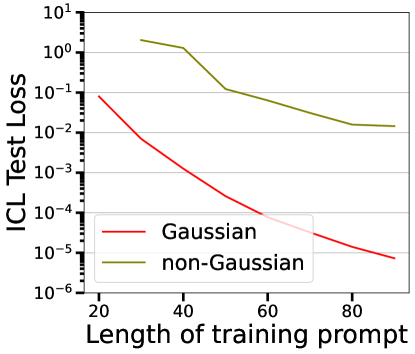
Figure 1: ICL loss of a 3-layer linear Transformer network trained under different context lengths. For each data point, the loss is computed with a test prompt from the same distribution as the training prompts. When the data distribution follows a non-Gaussian distribution (8), the learned linear Transformers are worse at learning linear target functions in context.

As illustrated by Figure 1, a key observation is that this non-Gaussian data distribution is more challenging for in-context learning compared to a Gaussian one. To understand why, the following result analyzes the optimization landscape.

Proposition 5.

Consider the distribution (8) as prescribed above, then for a one-layer linear Transformer $\mathsf{TF_{lin}}$, the self-attention weights that minimize the in-context learning loss $\mathcal{L}(\mathsf{TF_{lin}})$ satisfies

$$\mathbf{P}=\begin{bmatrix}0_{d\times d}&0\\ 0&1\end{bmatrix},\mathbf{Q}=-\begin{bmatrix}\Gamma&0\\ 0&0\end{bmatrix},$$

where $\Gamma$ is a $d\times d$ diagonal matrix whose entries are

$$\Gamma_{11}=\frac{n}{3(n-1)+5d+30},\;\;\Gamma_{jj}=\frac{n}{(n-1)+3d+18},\;\;j=2,\dots,d.$$ (9)

This can be viewed as a non-Gaussian counterpart to Theorem 1 in Ahn et al. (2024a), and the proof of this result can be found in Appendix E.

Remark 2.

In the limit as $n\to\infty$, the entries of $\Gamma$ converges to $(1/3,1,\dots,1)$, which is equal to the inverse of the second moment $\mathbb{E}[xx^{\top}]^{-1}$. Therefore, in the infinite data regime where the context length $n$ is very large, the optimal self-attention layer converges to solving an ordinary least squares.

In contrast, for a Gaussian distribution $x_{i}[1],\dots,x_{i}[d]\overset{i.i.d.}{\sim}\mathcal{N}(0,1)$, the work by Ahn et al. (2024b) shows that the optimal value of $\Gamma$ is given by $\Gamma=\mathrm{diag}(\frac{n}{(n-1)+d+2},\dots)$, which exhibits a much smaller dependence on the target function dimension $d$ compared to the non-Gaussian case. This means that, for the Gaussian case, the optimal $\Gamma$ converges to $\mathbb{E}[xx^{\top}]^{-1}$ much more quickly as $n$ increases. Under both distributions, as $n\to\infty$, the optimal linear Transformer approaches a least-square estimator, which would result in zero ICL loss. But our observations from both Proposition 5 and Figure 1 suggest that such convergence is much slower when the data distribution is non-Gaussian.

Because the output of the feed-forward layer in a bilinear Transformer would be non-Gaussian, the optimization landscape for quadratic functions (and nonlinear functions in general) is more complex than linear ones even for the same prompt distribution. This suggests that to effectively learn quadratic target functions in context, we require a longer context length $n$ relative to the problem dimension $d$.

5 Numerical experiments

5.1 Illustration of block-coordinate descent dynamics

To illustrate the block-coordinate descent update dynamics that we proposed in Section 4.2, we conduct a numerical experiment with a 12-layer bilinear Transformer, which, as previously shown, can perform up to 6 steps of block-coordinate descent updates. We set the parameters to $n=200$, $d=4$, and $\bar{d}=12$, resulting in $\binom{6}{2}=15$ distinct monomials for the quadratic function. The prompts are drawn according to a quadratic target function as described in Section 2.1. This setup implies that the embedding space is insufficient to compute the entire quadratic kernel with just one bilinear feed-forward layer.

In Figure 2, we analyze the in-context learning (ICL) performance of various sub-networks within the bilinear Transformer, where the first $2\ell$ layers correspond to $\ell$ steps of block-coordinate descent. We plot the ICL loss of the bilinear Transformer over 20000 training iterations. We observe that the ICL loss decreases significantly as the number of steps increases, which aligns with the behavior of a gradient-descent-based estimator. Additionally, we note that the ICL prediction after 2 steps is notably poor, indicating that the blocks selected by the trained Transformer have not yet covered all quadratic monomials after passing through two bilinear feed-forward layers. This outcome is expected given that our choice of $\bar{d}<\binom{d+2}{2}$ necessitates multiple steps to compute the full quadratic kernel.

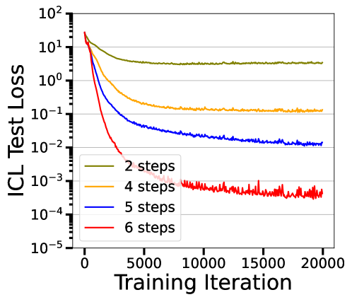
Figure 2: We evaluate the quadratic-function ICL performance of a 12-layer bilinear Transformer network, which can implement 6 steps of block-coordinate descent updates. The test losses of the trained Transformer are plotted over 20000 training iterations. Test loss is computed using a test prompt sampled independently of the training prompts. We compare the predictions from sub-networks that implement different numbers of update steps, so that the first $2\ell$ layers of the network implement $\ell$ steps of update.

5.2 Learning higher-degree polynomials in-context

The deep bilinear Transformer construction we discussed in Section 4.2 can also be used to generate higher-degree polynomial kernels. After passing through the first bilinear feed-forward layer, the intermediate prompt contains entries that are quadratic in the original prompt. The subsequent bilinear layer can then multiply these quadratic terms, yielding terms up to degree 4.

To illustrate this idea, we consider an example with $d=2,\bar{d}=6$. Suppose that, after passing through the first bilinear feed-forward layer, the columns of the prompt take the form $(1,x_{i}[1],x_{i}[2],x_{i}[1]x_{i}[2],0,0,y_{i})$. Let

$$\mathbf{W_{1}}=\begin{bmatrix}0&0&0&0&0&0\\ 0&0&0&0&0&0\\ 0&0&0&0&0&0\\ 0&0&0&0&0&0\\ 0&1&0&0&0&0\\ 0&0&0&1&0&0\end{bmatrix},\mathbf{W_{2}}=\begin{bmatrix}0&0&0&0&0&0\\ 0&0&0&0&0&0\\ 0&0&0&0&0&0\\ 0&0&0&0&0&0\\ 0&0&0&1&0&0\\ 0&0&0&1&0&0\end{bmatrix}.$$

Then, according to definition (3), the $i$-th column of the output from this bilinear layer takes the form $(1,x_{i}[1],x_{i}[2],x_{i}[1]x_{i}[2],x_{i}[1]^{2}x_{i}[2],x_{i}[1]^{2}x_{i}[2]^{2},y_{i})$, which includes both cubic and quartic terms. Since a deep bilinear Transformer contains multiple bilinear feed-forward layers, it can compute a higher-order polynomial kernel over multiple layers. Combining this idea with the construction used in Theorem 4 results in a Transformer that mimics block-coordinate descent updates over a higher-order polynomial kernel regression.

To illustrate this idea, we conduct an experiment where the target function is a cubic over 4 variables:

$$f(x;w)=w_{0}+\sum_{i=1}^{4}w_{i}x[i]+w_{12}x[1]x[2]+w_{23}x[2]x[3]+w_{34}x[3]x[4]$$

$$+w_{123}x[1]x[2]x[3]+w_{234}x[2]x[3]x[4],$$

where all of the coefficient $w$’s are drawn i.i.d. from $\mathcal{N}(0,1)$. We consider a 10-layer bilinear Transformer, which can perform up to 5 steps of block-coordinate descent updates. We set the parameters to $n=100$, $d=4$, and $\bar{d}=15$, noting that there are 35 distinct monomials in the cubic function class of 4 variables.

To demonstrate that the bilinear feed-forward layers compute the cubic terms, we also consider a “sparse” bilinear layer, whose parameters take the form

$$\mathbf{W_{i}}=\begin{bmatrix}0&0\\ \mathbf{\widetilde{W}_{i}}&0\end{bmatrix},\mathbf{\widetilde{W}_{i}}\in\mathbb{R}^{(\bar{d}-d-1)\times(d+1)}.$$ (10)

In this sparse form, the later bilinear feed-forward layers cannot reuse the nonlinear terms computed by the earlier bilinear layers.

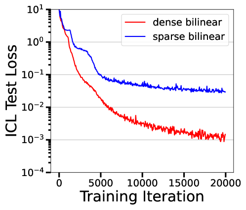
Figure 3: We evaluate the cubic-function ICL performance of two 10-layer bilinear Transformer networks, which can implement 5 steps of block-coordinate descent updates. The test losses of the trained Transformers are plotted over 20000 training iterations. Test loss is computed using a test prompt sampled independently of the training prompts. We compare predictions from a Transformer with standard dense bilinear layers (3) against one with sparse bilinear layer parameters (10). The sparse Transformer is specifically designed to avoid computing any cubic kernel features. The performance gap between the two models highlights that the standard bilinear Transformer is able to effectively implement cubic kernel regression.

Figure 3 shows the performance of a Transformer with the standard dense bilinear layer (3) and one with sparse bilinear parameters (10) after 20000 training iterations. We observe that the sparse bilinear Transformer performs significantly worse at learning this cubic function in-context. This suggests that the standard bilinear Transformer is indeed solving a higher-degree polynomial kernel regression.

6 Conclusion and future work

In this paper, we investigated the expressive power of Transformers to learn nonlinear target functions in-context. We first showed that previous works on linear Transformer architectures are insufficient for in-context learning (ICL) of nonlinear function classes. To overcome this challenge, we considered a deep bilinear Transformer, which alternates between self-attention and feed-forward layers — similar to recent Transformer designs in practice. Using quadratic function class as an example, we showed that a bilinear Transformer can perform nonlinear ICL by mimicking gradient-descent estimators on a kernel regression. Moreover, we discussed how our approach can be generalized to polynomial function classes. Finally, we highlighted challenges in applying bilinear Transformers to quadratic ICL and concluded that larger-scale Transformers are needed to learn nonlinear functions in-context, compared to linear ones.

Several directions for future research emerge from this study. First, we focused on single-head self-attention mechanisms, leaving the role of multiple attention heads in nonlinear ICL as an open question. Also, we found that Transformer’s ICL performance is highly sensitive to data distribution, which complicates nonlinear ICL tasks. We speculate that adding layer normalization could help address this issue.

Appendix A Proof of Proposition 1

We shall prove a more general statement. Recall that, in (1), the prompts are written as a matrix $Z\in\mathbb{R}^{(\bar{d}+1)\times(n+1)}$:

$$Z=\begin{bmatrix}1&1&\cdots&1&1\\ x_{1}&x_{2}&\cdots&x_{n}&x_{n+1}:=x_{\textsf{query}}\\ \mathbf{0}&\mathbf{0}&\cdots&\mathbf{0}&\mathbf{0}\\ y_{1}&y_{2}&\cdots&y_{n}&0\end{bmatrix},$$

where, for the purpose of this proposition, $x_{1},\dots,x_{n+1}\overset{i.i.d.}{\sim}\mathcal{N}(0,\Sigma)$ and $y_{i}=f(x_{i})$ for some fixed target function $f:\mathbb{R}^{d}\to\mathbb{R}$.

We note that, by defining

$$u_{i} =[1\;\;x_{i}\;\;\mathbf{0}],$$

$$g(u) =g(1,x_{i},\mathbf{0})=f(x),$$

the prompt (1) is a special case of the form

$$\zeta=\begin{bmatrix}u_{1}&u_{2}&\cdots&u_{n}&u_{n+1}:=u_{\mathsf{query}}\\ v_{1}&v_{2}&\cdots&v_{n}&0\end{bmatrix},$$ (11)

where, $u_{1},\dots,u_{n+1}\overset{i.i.d.}{\sim}\mathcal{D_{U}}$ for a distribution $\mathcal{D_{U}}$ over $\mathbb{R}^{\bar{d}}$ and $v_{i}=g(u_{i})$ for some fixed target function $g:\mathbb{R}^{\bar{d}}\to\mathbb{R}$.

Let $\hat{v}_{\mathsf{TF}}$ be the prediction of a Transformer $\mathsf{TF}$ with input $\zeta$. Then, Proposition 1 is simply a special case of showing that $\hat{v}_{\mathsf{TF}}$ is no better than the linear model over $u$.

Proposition 6.

Consider inputs $u_{1},\dots,u_{n+1}\overset{i.i.d.}{\sim}\mathcal{D_{U}}$ and any fixed target function $v_{i}=g(u_{i})$. The in-context learning prompts are sampled according to the form as described in (11). Then, for any linear Transformer $\mathsf{TF_{lin}}$ (of any number of layers), its expected prediction loss satisfies:

$$\mathbb{E}_{\mathcal{D_{U}}}[(\hat{v}_{\mathsf{TF}_{\mathsf{lin}}}+v_{\textsf{query}})^{2}]\geq\min_{\beta}\mathbb{E}_{\mathcal{D_{U}}}[(\left\langle u_{\textsf{query}},\beta\right\rangle+v_{\textsf{query}})^{2}].$$

Proof of Proposition 6.

Let the weights of the $\ell$th layer attention be

$$\mathbf{Q}^{(\ell)}=\begin{bmatrix}Q^{(\ell)}_{11}&Q^{(\ell)}_{12}\\ Q^{(\ell)}_{21}&Q^{(\ell)}_{22}\end{bmatrix},\mathbf{P}^{(\ell)}=\begin{bmatrix}P^{(\ell)}_{11}&P^{(\ell)}_{12}\\ P^{(\ell)}_{21}&P^{(\ell)}_{22}\end{bmatrix},$$

where $Q_{11}^{(\ell)}\in\mathbb{R}^{\bar{d}\times\bar{d}},Q_{12}^{\ell}\in\mathbb{R}^{\bar{d}},Q_{21}^{(\ell)}\in\mathbb{R}^{1\times\bar{d}}$ and $Q_{22}^{(\ell)}\in\mathbb{R}$, and similarly for $\mathbf{P}^{(\ell)}$.

Consider an input matrix

$$\zeta^{(0)}=\begin{bmatrix}u_{1}&u_{2}&\cdots&u_{n}&u_{n+1}:=u_{\mathsf{query}}\\ v_{1}&v_{2}&\cdots&v_{n}&0\end{bmatrix}:=\begin{bmatrix}U^{(0)}&u_{q}^{(0)}\\ {V^{(0)}}&v_{q}^{(0)}\end{bmatrix},$$

where the $U^{(0)}\in\mathbb{R}^{\bar{d}\times n},V^{(0)}\in\mathbb{R}^{1\times n},u_{q}^{(0)}\in\mathbb{R}^{\bar{d}}$ and $v_{q}^{(0)}\in\mathbb{R}$. And let $\zeta^{(\ell)}=\begin{bmatrix}U^{(\ell)}&u_{q}^{(\ell)}\\ {V^{(\ell)}}&v_{q}^{(\ell)}\end{bmatrix}$ be the output of the $\ell$th layer.

We shall use induction to show that:

• $U^{(\ell)}$ and $Y^{(\ell)}$ are independent of $u_{n+1}$.

• $u_{q}^{(\ell)}$ can be written as $A^{(\ell)}u_{n+1}$, where the matrix $A^{(\ell)}$ is independent of $u_{n+1}$.

• $v_{q}^{(\ell)}$ can be written as $\left\langle u_{n+1},b^{(\ell)}\right\rangle$, where $b^{(\ell)}$ is independent of $u_{n+1}$.

The base case when $\ell=0$ holds due to the independence of the columns. As for the inductive step, we compute the attention update directly. And for convenience, we shall drop superscripts $(\ell)$ and $(\ell-1)$ when they are clear from the context.

$$\zeta^{(\ell)} =\zeta^{(\ell-1)}+\frac{1}{n}(\mathbf{P}^{(\ell)}\zeta^{(\ell-1)})\begin{bmatrix}I_{n}&0\\ 0&0\end{bmatrix}({\zeta^{(\ell-1)}}^{\top}\mathbf{Q}^{(\ell)}{\zeta^{(\ell-1)}})$$

$$=\zeta^{(\ell-1)}+\frac{1}{n}\left(\begin{bmatrix}P_{11}^{(\ell)}&P_{12}^{(\ell)}\\ P_{21}^{(\ell)}&P_{22}^{(\ell)}\end{bmatrix}\begin{bmatrix}U^{(\ell-1)}&u_{q}^{(\ell-1)}\\ V^{(\ell-1)}&v_{q}^{(\ell-1)}\end{bmatrix}\right)\begin{bmatrix}I_{n}&0\\ 0&0\end{bmatrix}$$

$$\hskip 100.00015pt\left(\begin{bmatrix}{U^{(\ell-1)}}^{\top}&{V^{(\ell-1)}}^{\top}\\ {u_{q}^{(\ell-1)}}^{\top}&v_{q}^{(\ell-1)}\end{bmatrix}\begin{bmatrix}Q_{11}^{(\ell)}&Q_{12}^{(\ell)}\\ Q_{21}^{(\ell)}&Q_{22}^{(\ell)}\end{bmatrix}\begin{bmatrix}U^{(\ell-1)}&u_{q}^{(\ell-1)}\\ V^{(\ell-1)}&v_{q}^{(\ell-1)}\end{bmatrix}\right)$$

$$=\zeta+\frac{1}{n}\begin{bmatrix}P_{11}U+P_{21}V&P_{11}u_{q}+P_{12}v_{q}\\ P_{21}U+P_{22}V&P_{21}u_{q}+P_{22}y_{q}\end{bmatrix}\begin{bmatrix}I_{n}&0\\ 0&0\end{bmatrix}$$

$$\hskip 100.00015pt\left(\begin{bmatrix}U^{\top}Q_{11}+V^{\top}Q_{21}&U^{\top}Q_{12}+V^{\top}Q_{22}\\ u_{q}^{\top}Q_{11}+v_{q}Q_{21}&u_{q}^{\top}Q_{12}+v_{q}Q_{22}\end{bmatrix}\begin{bmatrix}U&u_{q}\\ V&v_{q}\end{bmatrix}\right)$$

$$=\zeta+\frac{1}{n}\begin{bmatrix}P_{11}U+P_{21}V&P_{11}u_{q}+P_{12}v_{q}\\ P_{21}U+P_{22}V&P_{21}u_{q}+P_{22}y_{q}\end{bmatrix}\begin{bmatrix}c_{1}&c_{2}\\ 0&0\end{bmatrix},$$

where

$$c_{1} =U^{\top}Q_{11}U+V^{\top}Q_{21}U+U^{\top}Q_{12}V+V^{\top}Q_{22}V$$

$$c_{2} =U^{\top}Q_{11}u_{q}+V^{\top}Q_{21}u_{q}+U^{\top}Q_{12}v_{q}+V^{\top}Q_{22}v_{q}.$$

Therefore, we have

$$U^{(\ell)} =U+\frac{1}{n}\left((P_{11}U+P_{21}V)(U^{\top}Q_{11}U+V^{\top}Q_{21}U+U^{\top}Q_{12}V+V^{\top}Q_{22}V)\right),$$

$$Y^{(\ell)} =Y+\frac{1}{n}\left((P_{21}U+P_{22}V)(U^{\top}Q_{11}U+V^{\top}Q_{21}U+U^{\top}Q_{12}V+V^{\top}Q_{22}V)\right),$$

$$u_{q}^{(\ell)} =u_{q}+\frac{1}{n}\left((P_{11}U+P_{21}V)(U^{\top}Q_{11}u_{q}+V^{\top}Q_{21}u_{q}+U^{\top}Q_{12}v_{q}+V^{\top}Q_{22}v_{q})\right)$$

$$=A^{(\ell-1)}u_{n+1}+\frac{1}{n}\left((P_{11}U+P_{21}V)C_{3}\right)u_{n+1},$$

$$v_{q}^{(\ell)} =v_{q}+\frac{1}{n}\left((P_{21}U+P_{22}V)(U^{\top}Q_{11}u_{q}+V^{\top}Q_{21}u_{q}+U^{\top}Q_{12}v_{q}+V^{\top}Q_{22}v_{q})\right)$$

$$={b^{(\ell-1)}}^{\top}u_{n+1}+\frac{1}{n}\left((P_{21}U+P_{22}V)C_{3}\right)u_{n+1},$$

where

$$C_{3} =U^{\top}Q_{11}A^{(\ell-1)}+V^{\top}Q_{21}A^{(\ell-1)}+U^{\top}Q_{12}{b^{(\ell-1)}}^{\top}+V^{\top}Q_{22}{b^{(\ell-1)}}^{\top}.$$

From here, it is not difficult to observe that our claim holds due to induction.

We define $\Lambda=\mathbb{E}_{\mathcal{D_{U}}}[uu^{\top}]$. Then, we compute the best linear fit as

$$\beta^{\star} :=\mathop{\mathrm{argmin}}_{\beta}\mathbb{E}\left(\left\langle\beta,u_{n+1}\right\rangle+v_{n+1}\right)^{2}$$ (12)

$$=\mathop{\mathrm{argmin}}_{\beta}\left\{\beta^{\top}\Lambda\beta+2\beta^{\top}\mathbb{E}_{\mathcal{D_{U}}}[uv]+\mathbb{E}_{\mathcal{D_{U}}}[v^{2}]\right\}$$

$$=\mathop{\mathrm{argmin}}_{\beta}\left\lVert\Lambda^{1/2}\beta+\Lambda^{-1/2}\mathbb{E}_{\mathcal{D_{U}}}[uv]\right\rVert_{2}^{2}$$

$$=-\Lambda^{-1}\mathbb{E}_{\mathcal{D_{U}}}[uv].$$

Finally, we rewrite the expected error of the prediction $\hat{v}_{\mathsf{TF_{lin}}}$ as

$$\mathbb{E}_{\mathcal{D_{U}}}\left[(\hat{v}+v_{n+1})^{2}\right] =\mathbb{E}_{\mathcal{D_{U}}}\left(\left(v_{n+1}+\left\langle\beta^{\star},u_{n+1}\right\rangle\right)-\left(\left\langle\beta^{\star},u_{n+1}\right\rangle-\hat{v}\right)\right)^{2}$$

$$\geq\mathbb{E}_{\mathcal{D_{U}}}\left(v_{n+1}+\left\langle\beta^{\star},u_{n+1}\right\rangle\right)^{2}-2\;\mathbb{E}_{\mathcal{D_{U}}}\left(v_{n+1}+\left\langle\beta^{\star},u_{n+1}\right\rangle\right)\left(\left\langle\beta^{\star},u_{n+1}\right\rangle-\hat{v}\right)$$

$$=\mathbb{E}_{\mathcal{D_{U}}}\left(v_{n+1}+\left\langle\beta^{\star},u_{n+1}\right\rangle\right)^{2}-2\;\mathbb{E}_{\mathcal{D_{U}}}\,\mathrm{tr}\left(u_{n+1}\left(v_{n+1}+\left\langle\beta^{\star},u_{n+1}\right\rangle\right)\left(\beta^{\star}-b^{(L)}\right)^{\top}\right)$$

$$=\mathbb{E}_{\mathcal{D_{U}}}\left(v_{n+1}+\left\langle\beta^{\star},u_{n+1}\right\rangle\right)^{2}-2\;\mathrm{tr}\left(\left(\mathbb{E}_{\mathcal{D_{U}}}[uv]+\Lambda\beta^{\star}\right)\left(\beta^{\star}-\mathbb{E}_{\mathcal{D_{U}}}[b^{(L)}]\right)^{\top}\right)$$

$$=\mathbb{E}_{\mathcal{D_{U}}}\left(v_{n+1}+\left\langle\beta^{\star},u_{n+1}\right\rangle\right)^{2},$$

where we used our claim above on the 3rd and 4th line, and we used that fact that $\beta^{\star}=-\Lambda^{-1}\mathbb{E}[uv]$ on the final line. Therefore, the population loss of the attention network’s prediction cannot be better than the best linear model over the original prompt. ∎

Appendix B Proof of Theorem 2

Recall that a bilinear Transformer block $\mathsf{BTFB}$ consists of a bilinear layer and then followed by a linear attention layer. The prompt $Z\in\mathbb{R}^{(\bar{d}+1)\times(n+1)}$ is specified by (1):

$$Z=\begin{bmatrix}1&1&\cdots&1&1\\ x_{1}&x_{2}&\cdots&x_{n}&x_{n+1}:=x_{\textsf{query}}\\ \mathbf{0}&\mathbf{0}&\cdots&\mathbf{0}&\mathbf{0}\\ y_{1}&y_{2}&\cdots&y_{n}&0\end{bmatrix},$$

with $x_{i}\overset{i.i.d.}{\sim}\mathcal{N}(0,\Sigma)$ and $y_{i}=f(x_{i})$ for target function $f$ is a quadratic function sampled according to Section 2.1. Then the output of the bilinear layer can be written in terms of slightly more general than the one in (11), where we replace the target function with a joint distribution on the inputs and labels.

$$\zeta=\begin{bmatrix}u_{1}&u_{2}&\cdots&u_{n}&u_{n+1}:=u_{\mathsf{query}}\\ v_{1}&v_{2}&\cdots&v_{n}&0\end{bmatrix}=:\begin{bmatrix}U&u_{q}\\ V&0\end{bmatrix},$$ (13)

where, $(u_{1},v_{1}),\dots,(u_{n+1},v_{n+1})\overset{i.i.d.}{\sim}\mathcal{D}$ for a distribution $\mathcal{D}$ over $\mathbb{R}^{\bar{d}}\times\mathbb{R}$. The distribution $\mathcal{D}$ is determined by the target function and our choice on the bilinear feed-forward layer, which we shall specify later.

Let $\hat{v}$ be the prediction of the linear self-attention layer with input $\zeta$. We first compute the prediction loss with a fixed bilinear feed-forward layer.

Lemma 7.

Consider $(u_{1},v_{1}),\dots,(u_{n+1},v_{n+1})\overset{i.i.d.}{\sim}\mathcal{D}$. The in-context learning prompts are sampled according to the form as described in (13). Let

$$\Lambda=\mathbb{E}_{\mathcal{D}}[uu^{\top}],\Phi=\mathrm{Cov}_{\mathcal{D}}[uv],\xi=\mathbb{E}_{\mathcal{D}}[uv].$$

Then, for a single-layer linear transformer with attention weights

$$\mathbf{P}=\begin{bmatrix}0_{d\times d}&0\\ 0&1\end{bmatrix},\mathbf{Q}=\begin{bmatrix}\Gamma&0\\ 0&0\end{bmatrix},$$

the error of the prediction $\hat{v}$ satisfies

$$\mathbb{E}_{\mathcal{D}}\left[(\hat{v}+v_{n+1})^{2}\right]=\min_{\beta}\mathbb{E}\left(\left\langle\beta,u_{n+1}\right\rangle+v_{n+1}\right)^{2}+\frac{1}{n}\mathrm{tr}\left(\Gamma\Lambda\Gamma^{\top}\Phi\right)+\xi^{\top}(\Gamma^{\top}+{\Lambda^{-1}})^{\top}\Lambda(\Gamma^{\top}+\Lambda^{-1})\xi.$$

Note that, if we choose $\Gamma=-\Lambda^{-1}$, then

$$\mathbb{E}_{\mathcal{D}}\left[(\hat{v}+v_{n+1})^{2}\right]=\min_{\beta}\mathbb{E}\left(\left\langle\beta,u_{n+1}\right\rangle+v_{n+1}\right)^{2}+\frac{1}{n}\mathrm{tr}\left(\Lambda^{-1}\Phi\right).$$

So, the next step is to choose an appropriate bilinear layer so that the quantity $\min_{\beta}\mathbb{E}\left(\left\langle\beta,u_{n+1}\right\rangle+v_{n+1}\right)^{2}$ is minimized for any quadratic target function $f$.

We choose the bilinear layer weights $\mathbf{W_{1}}$ and $\mathbf{W_{2}}$ as zero-one valued matrices. Recall that we have been using 1-based indexing in this paper. For every pair $1\leq j\leq k\leq d$, we set

$$\mathbf{W_{1}}\left[jd-\frac{1}{2}(j-1)j+k+1,j+1\right]=1,\quad\mathbf{W_{2}}\left[jd-\frac{1}{2}(j-1)j+k+1,k+1\right]=1.$$

This assigns one row of the bilinear layer’s output to have the values $x_{i}[i]x_{i}[k]$. The first argument of the index is equal to the lexicographic order of the pair $(j,k)$. In particular, under this choice, we get that

$$v_{i}=y_{i},\quad u_{i}=(1,x_{i}[1],\dots,x_{i}[d],x_{i}[1]^{2},\dots,x_{i}[1]x_{i}[d],x_{i}[2]^{2},\dots,x_{i}[2]x_{i}[d],\dots,x_{i}[d]^{2}),$$

where $u_{i}$ contains every possible monomial in a quadratic function of $x_{i}$. Then, for any quadratic target function $f$,

$$\min_{\beta}\mathbb{E}\left(\left\langle\beta,u_{n+1}\right\rangle+v_{n+1}\right)^{2}=0$$

by picking $-\beta$ equal to the coefficients of $f$.

In conclusion, with our choice of the bilinear layer and attention layer weights, the resulting in-context learning loss is

$$\mathcal{L}(\mathsf{BTFB})=\mathbb{E}_{f}[\mathbb{E}_{\mathcal{D}}(\hat{v}+v_{n+1})^{2}]=\mathbb{E}_{f}\frac{1}{n}\mathrm{tr}(\Lambda^{-1}\Phi)=\frac{1}{n}\mathrm{tr}\left(\Lambda^{-1}\mathbb{E}_{f}\Phi\right),$$

where $\Lambda^{-1}$ and $\mathbb{E}_{f}\Phi$ only depend on the value of $x_{i}$’s covariance $\Sigma$. So, $\mathcal{L}(\mathsf{BTFB})=O(1/n).$

B.1 Proof of Lemma 7

Recall that from our computation in (12)

$$\beta^{\star}:=\mathop{\mathrm{argmin}}_{\beta}\mathbb{E}\left(\left\langle\beta,u_{n+1}\right\rangle+v_{n+1}\right)^{2}=-\Lambda^{-1}\xi.$$

Let $\hat{\beta}=-\Gamma^{\top}\xi$. We rewrite the expected error as

$$\mathbb{E}\left[(\hat{v}+v_{n+1})^{2}\right] =\mathbb{E}\left(\left(v_{n+1}+\left\langle\beta^{\star},u_{n+1}\right\rangle\right)+\left(\left\langle\hat{\beta},u_{n+1}\right\rangle+\hat{v}\right)-\left(\left\langle\beta^{\star},u_{n+1}\right\rangle+\left\langle\hat{\beta},u_{n+1}\right\rangle\right)\right)^{2}$$

$$=\underbrace{\mathbb{E}\left(v_{n+1}+\left\langle\beta^{\star},u_{n+1}\right\rangle\right)^{2}}_{①}+\underbrace{\mathbb{E}\left(\left\langle\hat{\beta},u_{n+1}\right\rangle+\hat{v}\right)^{2}}_{②}+\underbrace{\mathbb{E}\left(\left\langle\beta^{\star},u_{n+1}\right\rangle+\left\langle\hat{\beta},u_{n+1}\right\rangle\right)^{2}}_{③}$$

$$\quad-\underbrace{2\;\mathbb{E}\left[\left(v_{n+1}+\left\langle\beta^{\star},u_{n+1}\right\rangle\right)\left(\left\langle\beta^{\star},u^{n+1}\right\rangle+\left\langle\hat{\beta},u_{n+1}\right\rangle\right)\right]}_{④}$$

$$\quad-\underbrace{2\;\mathbb{E}\left[\left(\left\langle\hat{\beta},u_{n+1}\right\rangle+\hat{v}\right)\left(\left\langle\beta^{\star},u_{n+1}\right\rangle+\left\langle\hat{\beta},u_{n+1}\right\rangle\right)\right]}_{⑤}$$

$$\quad+\underbrace{2\;\mathbb{E}\left[\left(v_{n+1}+\left\langle\beta^{\star},u_{n+1}\right\rangle\right)\left(\left\langle\hat{\beta},u_{n+1}\right\rangle+\hat{v}\right)\right]}_{⑥}$$

To further simplify these terms, we must first derive an explicit form for $\hat{v}$. To this end, we directly expand the attention layer:

$$\zeta^{+} =\zeta+\frac{1}{n}(\mathbf{P}\zeta)\begin{bmatrix}I_{n}&0\\ 0&0\end{bmatrix}({\zeta}^{\top}\mathbf{Q}{\zeta})$$

$$=\zeta+\frac{1}{n}\begin{bmatrix}0_{d\times d}&0\\ 0&1\end{bmatrix}\begin{bmatrix}U&u_{q}\\ V&0\end{bmatrix}\begin{bmatrix}I_{n}&0\\ 0&0\end{bmatrix}\left(\begin{bmatrix}U^{\top}&V^{\top}\\ u_{q}^{\top}&0\end{bmatrix}\begin{bmatrix}\Gamma&0\\ 0&0\end{bmatrix}\begin{bmatrix}U&u_{q}\\ V&0\end{bmatrix}\right)$$

$$=\zeta+\frac{1}{n}\begin{bmatrix}0&0\\ V&0\end{bmatrix}\begin{bmatrix}I_{n}&0\\ 0&0\end{bmatrix}\begin{bmatrix}U^{\top}&V^{\top}\\ u_{q}^{\top}&0\end{bmatrix}\begin{bmatrix}\Gamma U&\Gamma u_{q}\\ 0&0\end{bmatrix}$$

$$=\zeta+\frac{1}{n}\begin{bmatrix}0&0\\ V&0\end{bmatrix}\begin{bmatrix}U^{\top}\Gamma U&U^{\top}\Gamma u_{q}\\ 0&0\end{bmatrix}$$

$$=\begin{bmatrix}U&u_{q}\\ V+\frac{1}{n}VU^{\top}\Gamma U&\frac{1}{n}VU^{\top}\Gamma u_{q}\end{bmatrix}.$$

Therefore, we have that

$$\hat{v}=\frac{1}{n}VU^{\top}\Gamma u_{q}=\frac{1}{n}\left\langle\sum_{i=1}^{n}v_{i}u_{i},\Gamma u_{n+1}\right\rangle.$$

Then, for any fixed $u$, we have

$$\mathbb{E}\left[\left\langle\hat{\beta},u_{n+1}\right\rangle+\hat{v}\mid u_{n+1}=u\right]=\mathbb{E}\left[\frac{1}{n}\sum_{i=1}^{n}\Gamma^{\top}v_{i}u_{i}+\hat{\beta}\right]^{\top}u=0.$$

Therefore, under the tower property of expectation, terms ⑤ and ⑥ are 0.

As for term ④, we have

$$\frac{1}{2}④ =\mathbb{E}\left[\mathrm{tr}\left(u_{n+1}(v_{n+1}+\left\langle\beta^{\star},u_{n+1}\right\rangle)(\beta^{\star}+\hat{\beta})^{\top}\right)\right]$$

$$=\mathrm{tr}\left((\xi+\Lambda\beta^{\star})(\beta^{\star}+\hat{\beta})^{\top}\right)=0.$$

For term ②, we have

$$② =\mathbb{E}\left[\left(\frac{1}{n}\sum_{i=1}^{n}\Gamma^{\top}v_{i}u_{i}+\hat{\beta}\right)^{\top}u_{n+1}{u_{n+1}}^{\top}\left(\frac{1}{n}\sum_{i=1}^{n}\Gamma^{\top}v_{i}u_{i}+\hat{\beta}\right)\right]$$

$$=\mathbb{E}\left[\left(\frac{1}{n}\sum_{i=1}^{n}v_{i}u_{i}-\xi\right)^{\top}\Gamma u_{n+1}{u_{n+1}}^{\top}\Gamma^{\top}\left(\frac{1}{n}\sum_{i=1}^{n}v_{i}u_{i}-\xi\right)\right]$$

$$=\frac{1}{n}\mathrm{tr}\left(\Gamma\Lambda\Gamma^{\top}\Phi\right)$$

Latsly, for term ③, we have

$$③ =\mathbb{E}\left[(\beta^{\star}+\hat{\beta})^{\top}u_{n+1}{u_{n+1}}^{\top}(\beta^{\star}+\hat{\beta})\right]$$

$$=\xi^{\top}(\Gamma^{\top}+{\Lambda^{-1}})^{\top}\Lambda(\Gamma^{\top}+\Lambda^{-1})\xi.$$

Adding up these terms yields the desirable equation.

B.2 Verification of Proposition 1

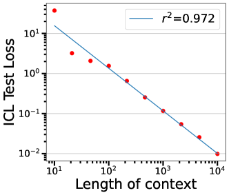
Figure 4: Quadratic ICL loss of the bilinear Transformer block construction associated with Proposition 2.

To verify Proposition 4, we apply the bilinear Transformer block construction associated with this result and compute its quadratic ICL loss at various context lengths $n$. Proposition 4 states that the ICL loss should scale inversely with $1/n$, which corresponds to a straight line on the log-log scale. This theoretical prediction is consistent with our empirical findings, shown in Figure 4, where the linear fit on the log-log scale yields an $r^{2}$ value of 0.97.

It’s important to note that our construction provides only an upper bound on the optimal ICL loss, and much smaller context lengths $n$ may suffice to achieve satisfactory performance. Additionally, multiple copies of the bilinear Transformer block can be stacked to improve ICL performance, enabling the Transformer to mimic multiple steps of gradient descent on quadratic kernel regression.

Appendix C Proof of Theorem 3

Recall that we consider inputs $x_{i}\overset{i.i.d.}{\sim}\mathcal{N}(0,I_{d})$. Let the output of the bilinear layer of $\mathsf{BTFB}$ be

$$\bar{Z}=\begin{bmatrix}\bar{x}_{1}&\bar{x}_{2}&\cdots&\bar{x}_{n}&\bar{x}_{n+1}\\ y_{1}&y_{2}&\cdots&y_{n}&0\end{bmatrix},$$

where $\bar{x}^{(i)}\in\mathbb{R}^{\bar{d}}$. Given Proposition 6, we have that

$$\mathcal{L}(\mathsf{BTFB})=\mathbb{E}_{w}\left[\mathbb{E}_{x}[(\hat{y}+y_{n+1})^{2}]\right]\geq\mathbb{E}_{w}\left[\min_{\beta}\mathbb{E}_{x}\left(y_{n+1}+\left\langle\beta,\bar{x}_{n+1}\right\rangle\right)^{2}\right].$$

Define inner product over random variables as $\left\langle u,v\right\rangle=\mathbb{E}[uv]$. Let

$$\begin{cases}v_{ij}=x_{n+1}[i]x_{n+1}[j]&\text{for }1\leq i<j\leq d,\\ v_{0j}=x_{n+1}[j]&\text{for }1\leq j\leq d.\\ \end{cases}$$

Note that $\mathbb{E}[v_{ij}^{2}]=1$ and for any $(i,j)\neq(i^{\prime},j^{\prime})$, we have that $\mathbb{E}[v_{ij}v_{i^{\prime}j^{\prime}}]=0$. Thus, $\{v_{ij}\}_{i<j}$ form an orthonormal set. Next, define the projection operator $P_{1}$ on a random variable $z$ as:

$$P_{1}(z)=\sum_{0\leq i<j\leq d}\mathbb{E}[zv_{ij}]v_{ij}.$$

Note that

$$\mathbb{E}[(z-P_{1}(z))v_{ij}]=\mathbb{E}[zv_{ij}]-\sum_{0\leq i^{\prime}<j^{\prime}\leq d}\mathbb{E}[zv_{i^{\prime}j^{\prime}}]\mathbb{E}[v_{ij}v_{i^{\prime}j^{\prime}}]=0.$$

So, we have $\mathbb{E}[(z-P_{1}(z))P_{1}(z)]=0.$ Recall that, for fixed coefficients $w$, we have

$$y_{n+1}=w_{0}+\sum_{i}w_{i}x_{n+1}[i]+\sum_{i}w_{ii}x_{n+1}[i]^{2}+\sum_{1\leq i<j\leq d}w_{ij}x_{n+1}[i]x_{n+1}[j].$$

For convenience, let $w_{0j}=w_{j}$. Then, it is not difficult to see that $P_{1}(y_{n+1})=\sum_{0\leq i<j\leq d}w_{ij}v_{ij}.$ Therefore, for any fixed $\beta$, we have that:

$$\mathbb{E}_{x}\left(y_{n+1}+\left\langle\beta,\bar{x}_{n+1}\right\rangle\right)^{2} \geq\mathbb{E}_{x}\left(P_{1}(y_{n+1})+P_{1}\left(\left\langle\beta,\bar{x}_{n+1}\right\rangle\right)\right)^{2}$$

$$=\mathbb{E}_{x}\left(\sum_{0\leq i<j\leq d}w_{ij}v_{ij}+\sum_{k=1}^{\bar{d}}\beta_{k}\sum_{0\leq i<j\leq d}\mathbb{E}\left[v_{ij}\bar{x}_{n+1}[k]\right]v_{ij}\right)^{2}$$

$$=\mathbb{E}_{x}\sum_{0\leq i<j\leq d}\left(\left(w_{ij}+\sum_{k=1}^{d}\beta_{k}\mathbb{E}\left[v_{ij}\bar{x}_{n+1}[k]\right]\right)v_{ij}\right)^{2}$$

$$=\sum_{0\leq i<j\leq d}\left(w_{ij}+\sum_{k=1}^{d}\beta_{k}\mathbb{E}\left[v_{ij}\bar{x}_{n+1}[k]\right]\right)^{2}.$$

Define a $\binom{d+1}{2}$-dimensional real vector space indexed by $\{(i,j):0\leq i<j\leq d\}$. Define vectors $\bar{w}$ and $\{u_{k}\}_{k=1}^{\bar{d}}$ on this vector space so that their are entries are:

$$\bar{w}=(w_{ij})_{i<j},u_{k}=\left(\mathbb{E}[v_{ij}\bar{x}_{n+1}[k]]\right)_{i<j}.$$

Let $P_{2}$ be the orthogonal projection onto the spanning space of $u_{k}$’s. Then, for any fixed $w$, the quantity above can be bounded by

$$\min_{\beta}\mathbb{E}_{x}\left(y_{n+1}+\left\langle\beta,\bar{x}_{n+1}\right\rangle\right)^{2}\geq\min_{\beta}\sum_{0\leq i<j\leq d}\left(w_{ij}+\sum_{k}\beta_{k}\mathbb{E}[v_{ij}\bar{x}_{n+1}[k]]\right)^{2}=\left\lVert\bar{w}-P_{2}(\bar{w})\right\rVert^{2}.$$

Now we take the expectation over $w$. Note that $\bar{w}\sim\mathcal{N}(0,I)$.

$$\mathbb{E}_{w}\left[\min_{\beta}\mathbb{E}_{x}\left(y_{n+1}+\left\langle\beta,\bar{x}_{n+1}\right\rangle\right)^{2}\right] \geq\mathbb{E}_{w}\left\lVert\bar{w}-P_{2}(\bar{w})\right\rVert^{2}$$

$$=\mathrm{tr}\left(\mathrm{Cov}[(I-P_{2})\bar{w}]\right)$$

$$=\mathrm{tr}(I-P_{2})\geq\binom{d+1}{2}-\bar{d}.$$

The last line holds because $P_{2}$ is an orthogonal projection matrix. Therefore, our claim holds.

Appendix D Proof of Theorem 4

We shall state a more complete version of Theorem 4, with the construction explicitly specified. Note that we use % to denote the remainder operator, with $a\%b$ having the range $\{1,\dots,b\}$.

Theorem 8.

For the quadratic function in-context learning problem as described in Section 2.1, we consider a $\mathsf{TF_{bilin}}$ with $2L$ layers and $\bar{d}=2d+1$. For $\ell=1,\dots,L$, we choose the $\ell$th bilinear feed-forward layer parameter as

$$\mathbf{W}_{1}^{(\ell)}=I_{d},\mathbf{W}_{2}^{(\ell)}=\begin{cases}E_{1}&\text{if }\ell=1,\\ -E_{(\ell-1)\%d}+E_{\ell\%d}&\text{otherwise},\\ \end{cases}$$

where $E_{j}$ denotes the matrix where the (in 1-based indexing) $(j+1)$st column is equal to all 1’s and 0 everywhere else. And we choose the $\ell$th self-attention layer parameters as

$$\mathbf{P}^{(2\ell)}=\begin{bmatrix}0_{d\times d}&0\\ 0&1\end{bmatrix},\mathbf{Q}^{(2\ell)}=\begin{bmatrix}\Gamma^{(\ell)}&0\\ 0&0\end{bmatrix}.$$

Then, for $\ell=1,\dots,L$, the forward pass of $\mathsf{TF_{bilin}}$ follows the form:

$$Z^{(0)} =Z=:\begin{bmatrix}1&1&\cdots&1\\ x_{1}&x_{2}&\cdots&x_{n+1}\\ 0&0&\cdots&0\\ y^{(0)}_{1}&y^{(0)}_{2}&\cdots&y^{(0)}_{n+1}\end{bmatrix},$$

$$Z^{(2\ell-1)} =\begin{bmatrix}1&1&\cdots&1\\ x_{1}&x_{2}&\cdots&x_{n+1}\\ x_{1}[\ell\%d]\cdot x_{1}&x_{2}[\ell\%d]\cdot x_{2}&\cdots&x_{n+1}[\ell\%d]\cdot x_{n+1}\\ y^{(\ell-1)}_{1}&y^{(\ell-1)}_{2}&\cdots&y^{(\ell-1)}_{n+1}\end{bmatrix},$$

$$Z^{(2\ell)} =\begin{bmatrix}1&1&\cdots&1\\ x_{1}&x_{2}&\cdots&x_{n+1}\\ x_{1}[\ell\%d]\cdot x_{1}&x_{2}[\ell\%d]\cdot x_{2}&\cdots&x_{n+1}[\ell\%d]\cdot x_{n+1}\\ y^{(\ell)}_{1}&y^{(\ell)}_{2}&\cdots&y^{(\ell)}_{n+1}\end{bmatrix}.$$

Furthermore, $\mathsf{TF_{bilin}}$ implements block-coordinate descent over a quadratic regression in the sense that

$$\hat{y}_{i}^{(\ell)}=y_{i}+\begin{bmatrix}1&x_{\mathsf{query}}\end{bmatrix}W^{(\ell)}\begin{bmatrix}1\\ x_{\mathsf{query}}\end{bmatrix},$$

where $W^{(\ell)}$ are iterates of the block-coordinate descent update (6) with initialization $W^{(0)}=0$, step sizes $\eta^{(\ell)}=-{\Gamma^{(\ell)}}^{\top}$ and blocks

$$b_{\ell}:=(1,x_{i}[1],\dots,x_{i}[d],x_{i}[1]x_{i}[\ell],\dots,x_{i}[d]x_{i}[\ell]).$$

Proof.

We shall prove the claim through induction. First, we consider the bilinear feed-forward layers. For the $\ell$-th bilinear layer, its input is $Z^{(2\ell-2)}$, and with our chosen weights, we have

$$Z^{(1)} =Z^{(0)}+\left(\begin{bmatrix}\mathbf{W_{1}}^{(1))}&0\\ 0&0\end{bmatrix}Z^{(0)}\right)\odot\left(\begin{bmatrix}\mathbf{W_{2}}^{(1)}&0\\ 0&0\end{bmatrix}Z^{(0)}\right)$$

$$=\begin{bmatrix}1&1&\cdots&1\\ x_{1}&x_{2}&\cdots&x_{n+1}\\ 0&0&\cdots&0\\ y^{(0)}_{1}&y^{(0)}_{2}&\cdots&y^{(0)}_{n+1}\end{bmatrix}+\begin{bmatrix}1&1&\cdots&1\\ x_{1}&x_{2}&\cdots&x_{n+1}\\ x_{1}[1]\cdot x_{1}&x_{2}[1]x_{2}&\cdots&x_{n+1}[1]\cdot x_{n+1}\\ y^{(0)}_{1}&y^{(0)}_{2}&\cdots&y^{(0)}_{n+1}\end{bmatrix}$$

$$=\begin{bmatrix}1&1&\cdots&1\\ x_{1}&x_{2}&\cdots&x_{n+1}\\ x_{1}[1]\cdot x_{1}&x_{2}[1]x_{2}&\cdots&x_{n+1}[1]\cdot x_{n+1}\\ y^{(0)}_{1}&y^{(0)}_{2}&\cdots&y^{(0)}_{n+1}\end{bmatrix}.$$

and for $\ell>1$,

$$Z^{(2\ell-1)} =Z^{(2\ell-2)}+\left(\begin{bmatrix}\mathbf{W_{1}}^{(\ell)}&0\\ 0&0\end{bmatrix}Z^{(2\ell-2)}\right)\odot\left(\begin{bmatrix}\mathbf{W_{2}}^{(\ell)}&0\\ 0&0\end{bmatrix}Z^{(2\ell-2)}\right)$$

$$=\begin{bmatrix}1&1&\cdots&1\\ x_{1}&x_{2}&\cdots&x_{n+1}\\ x_{1}[(\ell-1)\%d]\cdot x_{1}&x_{2}[(\ell-1)\%d]\cdot x_{2}&\cdots&x_{n+1}[(\ell-1)\%d]\cdot x_{n+1}\\ y^{(\ell-1)}_{1}&y^{(\ell-1)}_{2}&\cdots&y^{(\ell-1)}_{n+1}\end{bmatrix}$$

$$\quad+\begin{bmatrix}1&1&\cdots&1\\ x_{1}&x_{2}&\cdots&x_{n+1}\\ (x_{1}[\ell\%d]-x_{1}[(\ell-1)\%d])\cdot x_{1}&(x_{2}[\ell\%d]-x_{2}[(\ell-1)\%d])\cdot x_{2}&\cdots&(x_{n+1}[\ell\%d]-x_{n+1}[(\ell-1)\%d])\cdot x_{n+1}\\ y^{(\ell-1)}_{1}&y^{(\ell-1)}_{2}&\cdots&y^{(\ell-1)}_{n+1}\end{bmatrix}$$

$$=\begin{bmatrix}1&1&\cdots&1\\ x_{1}&x_{2}&\cdots&x_{n+1}\\ x_{1}[\ell\%d]\cdot x_{1}&x_{2}[\ell\%d]\cdot x_{2}&\cdots&x_{n+1}[\ell\%d]\cdot x_{n+1}\\ y^{(\ell-1)}_{1}&y^{(\ell-1)}_{2}&\cdots&y^{(\ell-1)}_{n+1}\end{bmatrix}.$$

Next, we turn our focus to the self-attention layers. For the $\ell$-th self-attention layer, its input is $Z^{(2\ell-1)}$. Denote

$$Z^{(2\ell-1)}=:\begin{bmatrix}X&x_{q}\\ Y&y_{q}\end{bmatrix},$$

where the $X\in\mathbb{R}^{\bar{d}\times n},Y\in\mathbb{R}^{1\times n},x_{q}\in\mathbb{R}^{\bar{d}}$ and $y_{q}\in\mathbb{R}$.

$$Z^{(2\ell)} =Z^{(2\ell-1)}+\frac{1}{n}\left(\mathbf{P}^{(\ell)}Z^{(2\ell-1)}\right)\begin{bmatrix}I_{n}&0\\ 0&0\end{bmatrix}\left({Z^{(2\ell-1)}}^{\top}\mathbf{Q}^{(\ell)}Z^{(2\ell-1)}\right)$$

$$=Z^{(2\ell-1)}+\frac{1}{n}\begin{bmatrix}0_{d\times d}&0\\ 0&1\end{bmatrix}\begin{bmatrix}X&x_{q}\\ Y&y_{q}\end{bmatrix}\begin{bmatrix}I_{n}&0\\ 0&0\end{bmatrix}\left(\begin{bmatrix}X^{\top}&Y^{\top}\\ x_{q}^{\top}&y_{q}\end{bmatrix}\begin{bmatrix}\Gamma^{(\ell)}&0\\ 0&0\end{bmatrix}\begin{bmatrix}X&x_{q}\\ Y&y_{q}\end{bmatrix}\right)$$

$$=Z^{(2\ell-1)}+\frac{1}{n}\begin{bmatrix}0&0\\ Y&y_{q}\end{bmatrix}\begin{bmatrix}I_{n}&0\\ 0&0\end{bmatrix}\begin{bmatrix}X^{\top}&V^{\top}\\ x_{q}^{\top}&y_{q}\end{bmatrix}\begin{bmatrix}\Gamma^{(\ell)}X&\Gamma^{(\ell)}x_{q}\\ 0&0\end{bmatrix}$$

$$=Z^{(2\ell-1)}+\frac{1}{n}\begin{bmatrix}0&0\\ Y&y_{q}\end{bmatrix}\begin{bmatrix}X^{\top}\Gamma X&X^{\top}\Gamma^{(\ell)}x_{q}\\ 0&0\end{bmatrix}$$

$$=\begin{bmatrix}X&x_{q}\\ Y+\frac{1}{n}YX^{\top}\Gamma^{(\ell)}X&y_{q}+\frac{1}{n}YX^{\top}\Gamma^{(\ell)}x_{q}\end{bmatrix}$$

$$=\begin{bmatrix}1&1&\cdots&1\\ x_{1}&x_{2}&\cdots&x_{n+1}\\ x_{1}[\ell\%d]\cdot x_{1}&x_{2}[\ell\%d]\cdot x_{2}&\cdots&x_{n+1}[\ell\%d]\cdot x_{n+1}\\ y^{(\ell)}_{1}&y^{(\ell)}_{2}&\cdots&y^{(\ell)}_{n+1}\end{bmatrix},$$

where

$$y_{i}^{(\ell)} =y_{i}^{(\ell-1)}+\left\langle\bar{x}_{i}^{(\ell)},\frac{1}{n}\sum_{i=1}^{n}{\Gamma^{(\ell)}}^{\top}\bar{x}_{i}^{(\ell)}y_{i}^{(\ell-1)}\right\rangle,$$

$$\bar{x}_{i}^{(\ell)} =(1,x_{i},x_{i}[\ell\%d]\cdot x_{i}).$$

Now we compare $y^{(\ell)}$ against the iterates of block coordinate descent through an induction argument. Let

$$f(x;W)=\begin{bmatrix}1&x\end{bmatrix}W\begin{bmatrix}1\\ x\end{bmatrix}.$$

Note that for any $j\in b_{\ell}$:

$$\partial w_{j}\left(\frac{1}{2n}\sum_{i=1}^{n}\left(f(x_{i},W^{(\ell-1)})+y_{i}\right)^{2}\right) =\frac{1}{n}\sum_{i=1}^{n}\left(f(x_{i},W^{(\ell-1)})+y_{i}\right)\widetilde{x}_{i}[j]$$

$$=\frac{1}{n}\sum_{i=1}^{n}y^{(\ell-1)}_{i}\widetilde{x}_{i}[j]$$

$$=\frac{1}{n}\sum_{i=1}^{n}y^{(\ell-1)}_{i}\bar{x}_{i}[j],$$

where we use $\widetilde{x}_{i}$ to denote the collection all quadratic monomials on $x_{i}$ and note that $\bar{x}_{i}=\widetilde{x}_{i}[b_{\ell}]$. Therefore,

$$y_{i}+f(x_{i},W^{(\ell)}) =y_{i}+f(x_{i},W^{(\ell-1)})-\left\langle\bar{x}_{i}^{(\ell)},\frac{1}{n}\sum_{i=1}^{n}\eta^{(\ell)}\bar{x}_{i}y^{(\ell-1)}_{i}\right\rangle,$$

which by induction is equal to $y_{i}^{(\ell)}$ if we set $\eta^{(\ell)}=-{\Gamma^{(\ell)}}^{\top}$. So we are done. ∎

Appendix E Proof of Proposition 5

Recall that we are concerned with a non-Gaussian distribution (8)

$$\begin{cases}v_{i}[1],\dots v_{i}[d]\overset{i.i.d.}{\sim}\mathcal{N}(0,1),\\ x_{i}[j]=v_{i}[1]v_{i}[j].\end{cases}$$

And the prompt takes the form

$$Z=\begin{bmatrix}x_{1}&x_{1}&\cdots&x_{1}&x_{n+1}:=x_{\textsf{query}}\\ y_{1}&y_{2}&\cdots&y_{n}&0\end{bmatrix}=:\begin{bmatrix}X&x_{q}\\ Y&0\end{bmatrix},$$

where $y_{i}=w^{\top}x_{i}$ for $w\sim\mathcal{N}(0,I_{d})$.

Let us write the attention weights as

$$\mathbf{Q}=\begin{bmatrix}Q_{11}&Q_{12}\\ Q_{21}&Q_{22}\end{bmatrix},\mathbf{P}=\begin{bmatrix}P_{11}&P_{12}\\ P_{21}&P_{22}\end{bmatrix},$$

where $Q_{11}\in\mathbb{R}^{d\times d},Q_{12}^{\ell}\in\mathbb{R}^{d},Q_{21}\in\mathbb{R}^{1\times d}$ and $Q_{22}\in\mathbb{R}$, and similarly for $\mathbf{P}$.

Then, we expand the definition of the self-attention layer:

$$\mathsf{attn}(Z) =Z+\frac{1}{n}(\mathbf{P}Z)\begin{bmatrix}I_{n}&0\\ 0&0\end{bmatrix}(Z^{\top}\mathbf{Q}Z)$$

$$=Z+\frac{1}{n}\left(\begin{bmatrix}P_{11}&P_{12}\\ P_{21}&P_{22}\end{bmatrix}\begin{bmatrix}X&x_{q}\\ Y&0\end{bmatrix}\right)\begin{bmatrix}I_{n}&0\\ 0&0\end{bmatrix}\left(\begin{bmatrix}X^{\top}&Y^{\top}\\ x_{q}^{\top}&0\end{bmatrix}\begin{bmatrix}Q_{11}&Q_{12}\\ Q_{21}&Q_{22}\end{bmatrix}\begin{bmatrix}X&x_{q}\\ Y&0\end{bmatrix}\right)$$

$$=Z+\frac{1}{n}\begin{bmatrix}P_{11}X+P_{21}Y&P_{11}x_{q}\\ P_{21}X+P_{22}Y&P_{21}x_{q}\end{bmatrix}\begin{bmatrix}I_{n}&0\\ 0&0\end{bmatrix}\left(\begin{bmatrix}X^{\top}Q_{11}+Y^{\top}Q_{21}&X^{\top}Q_{12}+Y^{\top}Q_{22}\\ x_{q}^{\top}Q_{11}&x_{q}^{\top}Q_{12}\end{bmatrix}\begin{bmatrix}X&x_{q}\\ Y&0\end{bmatrix}\right)$$

$$=Z+\frac{1}{n}\begin{bmatrix}P_{11}X+P_{21}Y&P_{11}x_{q}\\ P_{21}X+P_{22}Y&P_{21}x_{q}\end{bmatrix}\begin{bmatrix}*&X^{\top}Q_{11}x_{q}+Y^{\top}Q_{21}x_{q}\\ 0&0\end{bmatrix}.$$

So, $\hat{y}=\mathsf{attn}(Z)[d+1,n+1]=\frac{1}{n}(P_{21}X+P_{22}Y)(X^{\top}Q_{11}+Y^{\top}Q_{21})x_{q}$. If we let

$$H=\frac{1}{n}\sum_{i=1}^{n}\begin{bmatrix}x_{i}\\ y_{i}\end{bmatrix}[x_{i}^{\top}\;y_{i}],$$

$b^{\top}$ be the last row of $\mathbf{P}$, and $A$ be the first $d$ columns of $\mathbf{Q}$, we have

$$\hat{y}=b^{\top}HAx_{n+1}.$$

The ICL loss for this one-layer linear transformer $\mathsf{TF_{lin}}$ can be written as

$$\mathcal{L}(\mathsf{TF_{lin}})=:L(b,A)=\mathbb{E}_{Z}[(b^{\top}HAx_{n+1}+w^{\top}x_{n+1})^{2}].$$

And we can set every entry of $\mathbf{P},\mathbf{Q}$ outside of $b$ and $A$ as zero.

Define

$$\lambda_{j}=\mathbb{E}[x_{n+1}[j]^{2}]=\begin{cases}3&\text{if }j=1,\\ 1&\text{if }j\neq 1.\end{cases}$$

And note that $\mathbb{E}[x_{n+1}[j]x_{n+1}[j^{\prime}]]=0$ for any $j\neq j^{\prime}$. Let $A_{j}$ be the $j$th column of $A$ and denote $G_{j}=bA_{j}^{\top}$, then we can write the loss function as:

$$L(b,A)=\sum_{j=1}^{d}\lambda_{j}\mathbb{E}\left[(b^{\top}HA+w^{\top})[j]^{2}\right]=\sum_{j=1}^{d}\lambda_{j}\mathbb{E}\left[(b^{\top}HA_{j}+w_{j})^{2}\right]=\sum_{j=1}^{d}\lambda_{j}\mathbb{E}\left[(\mathrm{tr}(HG_{j}^{\top})+w_{j})^{2}\right].$$

Now, we minimize the loss $L$ with respect to $G_{j}$’s. Since $L$ is convex in $G_{j}$, it suffices to find matrices $G_{j}$’s so that

$$0=\nabla_{G_{j}}L=2\lambda_{j}\cdot\mathbb{E}[\underbrace{w_{j}H}_{①}+\underbrace{\mathrm{tr}(HG_{j}^{\top})H}_{②}].$$

Part ①:

We have

$$w_{j}H=\frac{1}{n}\sum_{i=1}^{n}\begin{bmatrix}x_{i}x_{i}^{\top}&x_{i}y_{i}\\ y_{i}x_{i}^{\top}&y_{i}^{2}\end{bmatrix}w_{j}.$$

Note that

• $\mathbb{E}[x_{i}x_{i}^{\top}w_{j}]=0$ because $\mathbb{E}[w_{j}]=0$.

• $\mathbb{E}[y_{i}^{2}w_{j}]=\mathbb{E}[\left\langle x_{i},w\right\rangle^{2}w_{j}]=0$ because $w_{j}$ is symmetric around 0.

• For $k\in\{1,\dots,d\}$,

  $$\mathbb{E}[y_{i}x_{i}[k]w_{j}]=\sum_{\ell=1}^{d}\mathbb{E}[w_{j}w_{\ell}x_{i}[\ell]x_{i}[k]]=\mathbb{E}\left[w_{j}w_{k}x_{i}[k]^{2}\right]=\lambda_{k}\cdot\mathds{1}_{\{j=k\}},$$

  where the second equality holds because $\mathbb{E}[x_{n+1}[j]x_{n+1}[j^{\prime}]]=0$ for any $j\neq j^{\prime}$ and the third equality holds because $w$ follows a standard normal distribution.

Let $e_{i,j}$ be the matrix whose $(i,j)$th entry is 1 and 0 elsewhere, then

$$\mathbb{E}[w_{j}H]=\lambda_{j}(e_{d+1,j}+e_{j,d+1}).$$

Part ②:

We compute

$$\mathbb{E}[\mathrm{tr}(He_{j,d+1})H] =\mathbb{E}\left[\frac{1}{n^{2}}\left(\sum_{i=1}^{n}y_{i}x_{i}[j]\right)\left(\sum_{i^{\prime}=1}^{n}\begin{bmatrix}x_{i^{\prime}}x_{i^{\prime}}^{\top}&x_{i^{\prime}}y_{i^{\prime}}\\ y_{i^{\prime}}x_{i^{\prime}}^{\top}&y_{i^{\prime}}^{2}\end{bmatrix}\right)\right]$$

$$=\mathbb{E}\left[\frac{1}{n^{2}}\left(\sum_{i=1}^{n}\left\langle x_{i},w\right\rangle x_{i}[j]\right)\left(\sum_{i^{\prime}=1}^{n}\begin{bmatrix}x_{i^{\prime}}x_{i^{\prime}}^{\top}&\left\langle x_{i^{\prime}},w\right\rangle x_{i^{\prime}}\\ \left\langle x_{i^{\prime}},w\right\rangle x_{i^{\prime}}^{\top}&\left\langle x_{i^{\prime}},w\right\rangle^{2}\end{bmatrix}\right)\right]$$

$$:=\begin{bmatrix}ⓐ&ⓑ\\ ⓑ^{\top}&ⓒ\end{bmatrix}.$$

Now we consider each of the submatrices:

• ⓐ = 0 because $\mathbb{E}[w]=0$.

• ⓒ = 0 because $w$ is symmetric around 0.

• Lastly,

  $$ⓑ[j^{\prime}] =\mathbb{E}\left[\frac{1}{n^{2}}\sum_{i,i^{\prime}}\left\langle w,x_{i}\right\rangle x_{i}[j]\left\langle w,x_{i^{\prime}}\right\rangle x_{i^{\prime}}[j^{\prime}]\right]$$

  $$=\mathbb{E}\left[\frac{1}{n^{2}}\sum_{i,i^{\prime}}x_{i}[j]x_{i^{\prime}}[j^{\prime}]\left(\sum_{k=1}^{d}x_{i}[d]x_{i^{\prime}}[d]\right)\right],$$

  where we first take the expectation over $w$ on the second line. Now, we do casework on the indices:

  • $i=i^{\prime},j=j^{\prime}$:

    $$\mathbb{E}\left[x_{i}[j]x_{i}[j]\left(\sum_{k=1}^{d}x_{i}[k]x_{i}[k]\right)\right] =\mathbb{E}\left[v_{i}[1]^{4}v_{i}[j]^{2}\left(\sum_{k=1}^{d}v_{i}[k]^{2}\right)\right]$$

    $$=\mathbb{E}\left[v_{i}[1]^{4}v_{i}[j]^{4}+\sum_{k\neq j}v_{i}[1]^{4}v_{i}[j]^{2}v_{i}[k]^{2}\right]$$

    $$=\begin{cases}105+15(d-1)=15d+90&\text{if }j=1,\\ 9+15+3(d-2)=3d+18&\text{if }j\neq 1.\end{cases}$$

  • $i=i^{\prime},j\neq j^{\prime}$:

    $$\mathbb{E}\left[x_{i}[j]x_{i}[j^{\prime}]\left(\sum_{k=1}^{d}x_{i}[k]x_{i}[k]\right)\right] =\mathbb{E}\left[v_{i}[1]^{4}v_{i}[j]v_{i}[j^{\prime}]\left(\sum_{k=1}^{d}v_{i}[k]^{2}\right)\right]=0.$$

  • $i\neq i^{\prime},j=j^{\prime}$:

    $$\mathbb{E}\left[x_{i}[j]x_{i^{\prime}}[j]\left(\sum_{k=1}^{d}x_{i}[k]x_{i^{\prime}}[k]\right)\right] =\mathbb{E}\left[v_{i}[1]^{2}v_{i^{\prime}}[1]^{2}v_{i}[j]v_{i^{\prime}}[j]\left(\sum_{k=1}^{d}v_{i}[k]v_{i^{\prime}}[k]\right)\right]$$

    $$=\mathbb{E}\left[v_{i}[1]^{2}v_{i^{\prime}}[1]^{2}v_{i}[j]^{2}v_{i^{\prime}}[j]^{2}\right]$$

    $$=\begin{cases}9&\text{if }j=1,\\ 1&\text{if }j\neq 1.\end{cases}.$$

  • $i\neq i^{\prime},j\neq j^{\prime}$:

    $$\mathbb{E}\left[x_{i}[j]x_{i^{\prime}}[j^{\prime}]\left(\sum_{k=1}^{d}x_{i}[k]x_{i^{\prime}}[k]\right)\right] =\mathbb{E}\left[v_{i}[1]^{2}v_{i^{\prime}}[1]^{2}v_{i}[j]v_{i^{\prime}}[j^{\prime}]\left(\sum_{k=1}^{d}v_{i}[k]v_{i^{\prime}}[k]\right)\right]$$

    $$=\sum_{k=1}^{d}\mathbb{E}\left[v_{i}[1]^{2}v_{i}[j]v_{i}[k]\right]\cdot\mathbb{E}\left[v_{i^{\prime}}[1]^{2}v_{i^{\prime}}[j^{\prime}]v_{i^{\prime}}[k]\right]=0.$$

  We used the fact that for a standard Gaussian, its 4th moment is 3, its 6th moment is 15 and its 8th moment is 105.

Therefore,

$$\mathbb{E}[\mathrm{tr}(He_{j,d+1})H] =c_{j}(e_{d+1,j}+e_{j,d+1})$$

$$\text{where }c_{j} =\begin{cases}(15d+90)n+3n(n-1)&\text{if }j=1.\\ (3d+18)n+n(n-1)&\text{if }j\neq 1.\end{cases}$$

Then, if we set $G_{j}=-\frac{\lambda_{j}}{c_{j}}e_{d+1,j}$, we have $①+②=0$. So, we found the optimal value of $G_{j}$’s.

We can achieve this choice of $G_{j}$’s if we set

$$b=\begin{bmatrix}0_{d}\\ 1\end{bmatrix},A_{j}[j]=-\frac{\lambda_{j}}{c_{j}}.$$

Therefore, the optimal self-attention parameters are

$$\mathbf{P} =\begin{bmatrix}0_{d\times d}&0\\ 0&1\end{bmatrix},\mathbf{Q}=-\begin{bmatrix}\Gamma&0\\ 0&0\end{bmatrix};$$

$$\text{where }\Gamma_{11} =\frac{n}{3(n-1)+5d+30},\quad\Gamma_{jj}=\frac{n}{(n-1)+3d+18},\quad j=2,\dots,d.$$

Appendix F Experiment Details

In our experiments, we trained our models using the Adam optimizer with a learning rate of $10^{-3}$ and no weight decay. For each iteration, we independently sample a batch of 4000 prompts.

• For the experiment in Figure 1, we solve a 10-dimensional ($d=10$) linear ICL task with a 3-layer linear Transformer. For various lengths of prompt $n$, the Transformer model is trained with either a Gaussian data distribution $x_{i}\sim\mathcal{N}(0,I)$ or a non-Gaussian distribution, as defined in (8). For each trained model, we compute its test loss by drawing a fresh in-distribution prompt with the same length $n$ and data distribution as during training.

• For the experiment in Figure 4, we directly use the bilinear Transformer block construction given in Appendix B without any training. We compute the test loss by drawing 100 prompts with $d=4,\bar{d}=15$.

• For the experiment in Figure 2, we train a single 12-layer bilinear Transformer with $n=200,d=4,\bar{d}=12$. We compute the predictions corresponding to different numbers of block-coordinate update steps by using the sub-network where the first $2\ell$ layers correspond to $\ell$ steps.

• For the experiment in Figure 3, we train two 10-layer bilinear Transformers with $n=100,d=4,\bar{d}=15$. For the model with sparse bilinear layers, we only train on the free weights as specified by (10), while the remaining entries of bilinear layer parameters are fixed to be zero.

All of the experiments were conducted on a single Nvidia V100 GPU.

References

- Ahn et al. [2024a] Kwangjun Ahn, Xiang Cheng, Hadi Daneshmand, and Suvrit Sra. Transformers learn to implement preconditioned gradient descent for in-context learning. Advances in Neural Information Processing Systems, 36, 2024a.
- Ahn et al. [2024b] Kwangjun Ahn, Xiang Cheng, Minhak Song, Chulhee Yun, Ali Jadbabaie, and Suvrit Sra. Linear attention is (maybe) all you need (to understand transformer optimization). In The Twelfth International Conference on Learning Representations, 2024b.
- Akyürek et al. [2023] Ekin Akyürek, Dale Schuurmans, Jacob Andreas, Tengyu Ma, and Denny Zhou. What learning algorithm is in-context learning? investigations with linear models. In International Conference on Learning Representations, 2023.
- Bahdanau et al. [2015] Dzmitry Bahdanau, Kyunghyun Cho, and Yoshua Bengio. Neural machine translation by jointly learning to align and translate. In International Conference on Learning Representations, 2015.
- Bai et al. [2024] Yu Bai, Fan Chen, Huan Wang, Caiming Xiong, and Song Mei. Transformers as statisticians: Provable in-context learning with in-context algorithm selection. Advances in neural information processing systems, 36, 2024.
- Bhattamishra et al. [2024] Satwik Bhattamishra, Arkil Patel, Phil Blunsom, and Varun Kanade. Understanding in-context learning in transformers and llms by learning to learn discrete functions. In International Conference on Learning Representations, 2024.
- Brown et al. [2020] Tom Brown, Benjamin Mann, Nick Ryder, Melanie Subbiah, Jared D Kaplan, et al. Language models are few-shot learners. Advances in neural information processing systems, 2020.
- Cheng et al. [2024] Xiang Cheng, Yuxin Chen, and Suvrit Sra. Transformers implement functional gradient descent to learn non-linear functions in context. In Forty-first International Conference on Machine Learning, 2024.
- Dai et al. [2023] Damai Dai, Yutao Sun, Li Dong, Yaru Hao, Shuming Ma, Zhifang Sui, and Furu Wei. Why can gpt learn in-context? language models secretly perform gradient descent as meta-optimizers. In Findings of the Association for Computational Linguistics: ACL 2023, pages 4005–4019, 2023.
- Dao and Gu [2024] Tri Dao and Albert Gu. Transformers are ssms: Generalized models and efficient algorithms through structured state space duality. In International Conference on Machine Learning, 2024.
- Dauphin et al. [2017] Yann N Dauphin, Angela Fan, Michael Auli, and David Grangier. Language modeling with gated convolutional networks. In International conference on machine learning, pages 933–941. PMLR, 2017.
- Dosovitskiy et al. [2021] Alexey Dosovitskiy, Lucas Beyer, Alexander Kolesnikov, Dirk Weissenborn, et al. An image is worth 16x16 words: Transformers for image recognition at scale. In International Conference on Learning Representations, 2021.
- Edelman et al. [2022] Benjamin L Edelman, Surbhi Goel, Sham Kakade, and Cyril Zhang. Inductive biases and variable creation in self-attention mechanisms. In International Conference on Machine Learning, pages 5793–5831. PMLR, 2022.
- Garg et al. [2022] Shivam Garg, Dimitris Tsipras, Percy S Liang, and Gregory Valiant. What can transformers learn in-context? a case study of simple function classes. Advances in Neural Information Processing Systems, 35:30583–30598, 2022.
- Giannou et al. [2023] Angeliki Giannou, Shashank Rajput, Jy-yong Sohn, Kangwook Lee, Jason D Lee, and Dimitris Papailiopoulos. Looped transformers as programmable computers. In International Conference on Machine Learning, pages 11398–11442. PMLR, 2023.
- Guo et al. [2024] Tianyu Guo, Wei Hu, Song Mei, Huan Wang, Caiming Xiong, Silvio Savarese, and Yu Bai. How do transformers learn in-context beyond simple functions? a case study on learning with representations. In The Twelfth International Conference on Learning Representations, 2024.
- Li et al. [2023] Yingcong Li, Muhammed Emrullah Ildiz, Dimitris Papailiopoulos, and Samet Oymak. Transformers as algorithms: Generalization and stability in in-context learning. In International Conference on Machine Learning, pages 19565–19594. PMLR, 2023.
- Lin et al. [2024] Licong Lin, Yu Bai, and Song Mei. Transformers as decision makers: Provable in-context reinforcement learning via supervised pretraining. In The Twelfth International Conference on Learning Representations, 2024.
- Mahankali et al. [2024] Arvind Mahankali, Tatsunori B Hashimoto, and Tengyu Ma. One step of gradient descent is provably the optimal in-context learner with one layer of linear self-attention. In International Conference on Learning Representations, 2024.
- Min et al. [2022] Sewon Min, Mike Lewis, Luke Zettlemoyer, and Hannaneh Hajishirzi. Metaicl: Learning to learn in context. In Proceedings of the 2022 Conference of the North American Chapter of the Association for Computational Linguistics: Human Language Technologies, pages 2791–2809, 2022.
- Mnih and Hinton [2007] Andriy Mnih and Geoffrey Hinton. Three new graphical models for statistical language modelling. In Proceedings of the 24th international conference on Machine learning, pages 641–648, 2007.
- Olsson et al. [2022] Catherine Olsson, Nelson Elhage, Neel Nanda, Nicholas Joseph, Nova DasSarma, Tom Henighan, et al. In-context learning and induction heads. arXiv preprint arXiv:2209.11895, 2022.
- OpenAI [2023] OpenAI. Gpt-4 technical report. arXiv preprint arXiv:2303.08774, 2023.
- Pérez et al. [2021] Jorge Pérez, Pablo Barceló, and Javier Marinkovic. Attention is turing-complete. Journal of Machine Learning Research, 22(75):1–35, 2021.
- Radford et al. [2023] Alec Radford, Jong Wook Kim, Tao Xu, Greg Brockman, Christine McLeavey, and Ilya Sutskever. Robust speech recognition via large-scale weak supervision. In International conference on machine learning, pages 28492–28518. PMLR, 2023.
- Shazeer [2020] Noam Shazeer. Glu variants improve transformer. arXiv preprint arXiv:2002.05202, 2020.
- Vaswani et al. [2017] Ashish Vaswani, Noam Shazeer, Niki Parmar, Jakob Uszkoreit, Llion Jones, et al. Attention is all you need. Advances in neural information processing systems, 30, 2017.
- Von Oswald et al. [2023] Johannes Von Oswald, Eyvind Niklasson, Ettore Randazzo, João Sacramento, et al. Transformers learn in-context by gradient descent. In International Conference on Machine Learning. PMLR, 2023.
- Wei et al. [2022a] Colin Wei, Yining Chen, and Tengyu Ma. Statistically meaningful approximation: a case study on approximating turing machines with transformers. Advances in Neural Information Processing Systems, 35:12071–12083, 2022a.
- Wei et al. [2022b] Jason Wei, Yi Tay, Rishi Bommasani, Colin Raffel, Barret Zoph, Sebastian Borgeaud, Dani Yogatama, Maarten Bosma, Denny Zhou, Donald Metzler, et al. Emergent abilities of large language models. Transactions on Machine Learning Research, 2022b.
- Wu et al. [2024] Jingfeng Wu, Difan Zou, Zixiang Chen, Vladimir Braverman, Quanquan Gu, and Peter Bartlett. How many pretraining tasks are needed for in-context learning of linear regression? In The Twelfth International Conference on Learning Representations, 2024.
- Yang et al. [2024a] Songlin Yang, Bailin Wang, Yikang Shen, Rameswar Panda, and Yoon Kim. Gated linear attention transformers with hardware-efficient training. In International Conference on Machine Learning. PMLR, 2024a.
- Yang et al. [2024b] Tong Yang, Yu Huang, Yingbin Liang, and Yuejie Chi. In-context learning with representations: Contextual generalization of trained transformers. arXiv preprint arXiv:2408.10147, 2024b.
- Yang et al. [2023] Zhengyuan Yang, Linjie Li, Kevin Lin, Jianfeng Wang, Chung-Ching Lin, Zicheng Liu, and Lijuan Wang. The dawn of lmms: Preliminary explorations with gpt-4v (ision). arXiv preprint arXiv:2309.17421, 2023.
- Zhang et al. [2024a] Ruiqi Zhang, Spencer Frei, and Peter L Bartlett. Trained transformers learn linear models in-context. Journal of Machine Learning Research, 25(49):1–55, 2024a.
- Zhang et al. [2024b] Ruiqi Zhang, Jingfeng Wu, and Peter L Bartlett. In-context learning of a linear transformer block: benefits of the mlp component and one-step gd initialization. Advances in Neural Information Processing Systems, 2024b.