Semantic Communication with Entropy-and-Channel-Adaptive Rate Control

Abstract

Although significant improvements in transmission efficiency have been achieved, existing semantic communication (SemCom) methods typically use a fixed transmission rate for varying channel conditions and transmission contents, leading to performance degradation under harsh channel conditions. To address these challenges, we propose a novel SemCom method for wireless image transmission that integrates entropy-and-channel-adaptive rate control mechanism, specifically designed for multi-user multiple-input multiple-output (MU-MIMO) fading channels. Unlike existing methods, our system dynamically adjusts transmission rates by leveraging the entropy of feature maps, channel state information (CSI), and signal-to-noise ratio (SNR), ensuring optimal communication resource usage. It incorporates feature map pruning, channel attention, spatial attention, and multi-head self-attention (MHSA) to effectively prioritize critical semantic features while minimizing unnecessary transmission overhead. Experimental results demonstrate that the proposed system outperforms separated source and channel coding and deep joint source and channel coding (deep JSCC), in terms of rate-distortion performance, flexibility, and robustness, particularly in challenging scenarios such as low SNR, imperfect CSI, and inter-user interference.

I Introduction

In recent years, semantic communication (SemCom) has garnered significant academic interest as an alternative communication paradigm with the potential to surpass the Shannon capacity limit [2, 3]. SemCom [4] enhances bandwidth efficiency by selectively extracting and transmitting only crucial information relevant to specific transmission tasks, i.e., semantic information, while disregarding non-essential content. This makes SemCom a promising solution for wireless communication applications that generate large amounts of data traffic, such as smart transportation [5], video conferencing [6], and autonomous driving [7]. Existing SemCom approaches typically leverage advanced deep learning techniques to extract semantic information from source data at the transmitter and reconstruct the source data at the receiver through end-to-end training. These approaches have demonstrated excellent performance in transmitting various data types, including text [8, 9, 10, 11], speech [12, 13, 14], images/videos [15, 16, 17, 18, 19, 20, 21], and multimodal data [22, 23, 24, 25].

However, current SemCom methods usually map source data directly into complex-valued channel input symbols, treating all symbols with equal importance when allocating communication resources. This approach fails to account for the varying significance of different transmitted symbols based on the specific transmission task. Furthermore, existing SemCom systems typically employ a fixed neural network model for encoding and decoding, resulting in a constant compression ratio. This limitation hinders the adaptability of these systems to changing channel conditions and prevents them from fully utilizing communication resources to enhance transmission performance.

Regarding the varying importance of semantic features, Guo et al. [26] considered cloud chat robot-to-human SemCom systems and exploited pre-trained language models to quantify the semantic importance of data frames and words in input sentences. They allocated the transmission power of each data frame at the physical layer based on the quantified semantic importance to minimize semantic loss. Liu et al. [27] proposed a semantic importance measurement method for an OFDM digital SemCom system, taking into account both the correlation between semantic features and tasks, and the correlation among different semantic features. They employed a greedy algorithm to allocate more reliable sub-channels for the transmission of semantic features with higher semantic importance. Gao et al. [28] proposed a metric called semantic value to measure the importance of semantic features for text transmission. This metric is defined to follow Zipf’s distribution, meaning that the importance of semantic features is related to word frequency. The transmitter ranks the semantic triples according to their semantic value and transmits only those with high semantic values. These studies consider the importance of semantic features, allowing important semantic features to be prioritized for transmission to improve communication performance. However, the high complexity of these methods in calculating the importance of semantic features results in a significant increase in latency.

Regarding the second aspect, several studies have been conducted on multi-rate SemCom systems. Kurka et al. [29] [30] considered adaptive bandwidth design for wireless image transmission SemCom systems over single-input single-output (SISO) AWGN channels and slow fading channels. They considered the scenario in which images are transmitted progressively in layers over time or frequency, incrementally improving the reconstruction performance. This approach enables a single model to transmit semantic features at several predetermined rates and to reconstruct the source image with different peak signal-to-noise ratio (PSNR) performances. Bian et al. [31] considered adaptive bandwidth design over SISO AWGN channels. They treated the channel SNR and the bandwidth ratio as channel state information, feeding them into the model, and trained the model using different channel SNRs as well as several predetermined rates. Additionally, during model training, they adjusted the weights of the reconstruction losses based on the reconstruction performance at different rates. The proposed model can adapt to different SNRs and bandwidth ratios.

Further, Yang et al. [32] developed an adaptive-rate SemCom system over SISO AWGN channels. Their proposed scheme utilizes a policy network that automatically adjusts the transmission rate based on the channel SNR and the content of the source image to an arbitrary value within a certain range. Zhang et al. [33] proposed a predictive and adaptive coding framework for SemCom systems over SISO AWGN channels. Their system can predict the performance of a single image transmission task based on channel conditions, compression ratio, and image contents, which further allows for the prediction of the optimal compression ratio. Subsequently, the system can automatically adjust the coding rate according to the channel conditions and the predicted optimal compression ratio. Gao et al. [34] proposed an adaptive modulation and retransmission scheme for SemCom systems over SISO fading channels. Their system is able to adaptively select a suitable modulation scheme based on robustness probability threshold constraints, thereby maximizing the transmission efficiency while ensuring task performance. Wang et al. [35] proposed an adaptive-rate SemCom system for video transmission over SISO AWGN channels that can allocate limited channel bandwidth to each video frame. During training, the system learns a variable-length coding method by minimizing the end-to-end transmission rate-distortion performance under given perceptual quality metrics. He et al. [36] proposed a multi-modal SemCom framework with a rate-adaptive coding mechanism over SISO AWGN channels. They defined the semantic importance of different modalities for semantic tasks based on their noise sensitivity and assigned coding rates to different modalities according to their semantic importance and the channel conditions, aiming to minimize the inference delay.

Nevertheless, existing studies on rate-adaptive SemCom exhibit several limitations. Some proposed adaptive bandwidth SemCom systems are trained using only a single channel SNR. This results in performance degradation if there is a significant difference between the actual channel SNR and the training channel SNR, and these systems are unable to automatically adjust the transmission rate according to the channel conditions (e.g., channel SNR or channel gain). Additionally, the transmission rates in the SemCom systems proposed in [29, 30, 31, 34, 35] are limited to several predetermined values, lacking rate flexibility. Furthermore, these studies primarily focus on simple SISO channels, with little research on adaptive rate control schemes for SemCom systems in multi-user MIMO (MU-MIMO) scenarios. Finally, while these studies aim to reduce the number of feature maps to be transmitted, they overlook the possibility of reducing the length of each feature map as well.

Compared to SISO systems, MIMO wireless communication [37] enables the parallel transmission of multiple data streams through spatial multiplexing, thereby significantly increasing throughput. Consequently, it is a crucial technology in modern wireless communication systems and serves as a core component of technologies such as WiFi, 4G LTE, and 5G. MIMO communication systems can be broadly categorized into two types based on whether they involve feedback of the channel state information (CSI) from the receiver: open-loop and closed-loop systems. In this paper, we focus on closed-loop MIMO systems, where the CSI is estimated at the receiver and then fed back to the transmitter.

To overcome the limitations of existing rate-adaptive SemCom approaches identified earlier, we propose a wireless image transmission semantic communication system with entropy- and channel-adaptive rate control for MU-MIMO fading channels. Our system dynamically selects the optimal transmission rates for multiple users based on feature maps and their entropies, as well as the CSI and channel SNR, thereby minimizing unnecessary transmission overhead. Specifically, we introduce two policy networks at the transmitter side that determine which feature maps to send and the ratio of those maps should be pruned. Given that attention mechanisms [38] are widely applied in fields like computer vision (CV) [39] and natural language processing (NLP) [40], and have shown promise in SemCom applications [41, 42], our system also incorporates channel attention, spatial attention [43], and multi-head self-attention (MHSA) mechanisms [44] during feature map extraction and image reconstruction. This integration enhances the system’s ability to capture critical semantic information and reconstruct source images effectively. The main contributions of this paper are as follows:

$\bullet$ Entropy-Aware Transmission: On one hand, we maximize the average entropy of the feature maps during training to increase the average amount of information carried by each transmitted symbol, thereby enhancing the transmission efficiency. On the other hand, the entropies of the feature maps are also leveraged to select the feature maps to transmit, enabling adaptive transmission rate to the semantic contents.

$\bullet$ Entropy and Channel Adaptive Rate Control: We introduce a rate-adaptive control mechanism that takes into account both the channel conditions and the entropy of feature maps. Specifically, we introduce two policy networks: one selects the feature maps to transmit according to their entropies, channel SNR, and CSI, while the other determines the pruning ratio of each feature map based on the channel conditions. This mechanism effectively improves both transmission efficiency and adaptability to various channel conditions.

$\bullet$ Feature and Channel Attention: Our method also incorporates channel attention, spatial attention, and multi-head self-attention (MHSA) mechanisms in order to capture critical semantic information and reconstruct source images effectively.

Experimental results demonstrate that the proposed SemCom method outperforms existing schemes in terms of image transmission and effectively adapts to different channel conditions with the proposed rate control mechanism. It also demonstrates the effectiveness of the entropy and attention mechanisms, the entropy and channel adaptive rate control mechanism, and the robustness of the proposed method to imperfect CSI and inter-user interference.

The rest of the paper is organized as follows. Section II introduces our system model. Section III introduces the detailed components of our proposed system. Section IV presents the experimental settings and performance evaluation. Finally, Section VI concludes our paper.

Notation: $\mathbb{R}^{n\times m}$ and $\mathbb{C}^{n\times m}$ represent sets of real and complex matrices of size $n\times m$, respectively. $\mathbb{E}(\cdot)$ denotes the expected value of a given variable. $H(\cdot)$ represents the entropy of a given variable. $\left.\textbf{x}\right.\sim\mathcal{C}\mathcal{N}\left(\mu,\sigma^{2}\right)$ means variable x follows a circularly-symmetric complex Gaussian distribution with mean $\mu$ and variance $\sigma^{2}$. $(\cdot)^{T}$, $(\cdot)^{H}$ and $(\cdot)^{-1}$ denote transposition, Hermitian, and inverse operation on a matrix, respectively.

II System Model

In this paper, we consider the semantic communication problem in a MU-MIMO uplink scenario, where there are $K$ single-antenna transmitters and a receiver equipped with $M$ antennas. Each user transmits its own image to the receiver through the MU-MIMO fading channels as shown in Fig. 1.

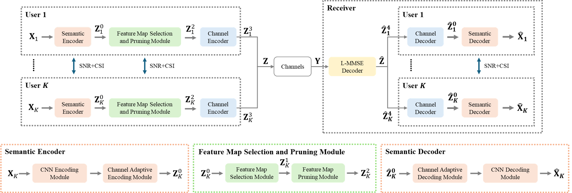
Figure 1: The overall architecture of the proposed SemCom system.

Each transmitter consists of a semantic encoder, a feature map selection and pruning module, and a channel encoder. The semantic encoder at each user extracts and encodes semantic features from the source image, denoted by

$$\textbf{Z}_{k}^{0}=f_{\mathrm{se},k}\left({\textbf{X}_{k},\hat{\textbf{h}}_{k},\hat{\mathrm{SNR}};\bm{\theta}_{k}^{\mathrm{se}}}\right),k=1\cdots K,$$ (1)

where $f_{\mathrm{se},k}(\cdot)$ represents the semantic encoder at user $k$, $\bm{\theta}_{k}^{\mathrm{se}}$ refers to its learnable parameters, $\textbf{X}_{k}$ is the image to transmit, $\hat{\textbf{h}}_{k}$ is the estimated CSI, $\hat{\mathrm{SNR}}$ is the estimated channel SNR, $\textbf{Z}_{k}^{0}$ is the corresponding output feature maps. Notably, $\hat{\textbf{h}}_{k}$ and $\hat{\mathrm{SNR}}$ can be obtained through the transmission of pilot signals. Specifically, the transmitter first sends pilot signals, after which the receiver estimates $\hat{\textbf{h}}_{k}$ and $\hat{\mathrm{SNR}}$ based on the received pilot signals and feeds these estimates back to the transmitter. The computation of $\hat{\textbf{h}}_{k}$ and $\hat{\mathrm{SNR}}$ will be discussed later.

Then the feature maps $\textbf{Z}_{k}^{0}$, together with their processed entropy $H^{\prime}(\textbf{Z}_{k}^{0})$ (to be introduced later), the estimated CSI $\hat{\textbf{h}}_{k}$, and the estimated channel SNR, are input to the feature map selection module, which selects a subset of important feature maps for transmission, denoted by

$$\textbf{Z}_{k}^{1}=f_{\mathrm{fms},k}\left(\textbf{Z}_{k}^{0},H^{\prime}\left(\textbf{Z}_{k}^{0}\right),\hat{\textbf{h}}_{k},\hat{\mathrm{SNR}};\bm{\theta}_{k}^{\mathrm{fms}}\right),$$ (2)

where $f_{\mathrm{fms},k}(\cdot)$ represents the feature map selection module at user $k$, $\bm{\theta}_{k}^{\mathrm{fms}}$ refers to its learnable parameters. The selected feature maps $\textbf{Z}_{k}^{1}$, together with $\hat{\textbf{h}}_{k}$, and the estimated channel SNR are fed into the feature map pruning module, which further prunes each feature map to generate sparse feature maps, $\textbf{Z}_{k}^{2}$, and a binary matrix $\textbf{M}_{\mathrm{p},k}$, that records the positions of the pruned pixels, denoted by

$$\textbf{Z}_{k}^{2},\textbf{M}_{\mathrm{p},k}=f_{\mathrm{fmp},k}\left(\textbf{Z}_{k}^{1},\hat{\textbf{h}}_{k},\hat{\mathrm{SNR}};\bm{\theta}_{k}^{\mathrm{fmp}}\right),$$ (3)

where $f_{\mathrm{fmp},k}(\cdot)$ represents the feature map pruning module, $\bm{\theta}_{k}^{\mathrm{fmp}}$ refers to its learnable parameters.

Both $\textbf{Z}_{k}^{2}$ and $\textbf{M}_{\mathrm{p},k}$ are subsequently fed into the channel encoder, which generates the complex-valued channel input signal $\textbf{Z}_{k}^{3}$ that meets the average power constraint, denoted as

$$\textbf{Z}_{k}^{3}=f_{\mathrm{ce},k}\left(\textbf{Z}_{k}^{2},\textbf{M}_{\mathrm{p},k}\right),$$ (4)

where $f_{\mathrm{ce},k}$ represents the channel encoder at user $k$. Next, $\textbf{Z}_{k}^{3}$ are transmitted over a MU-MIMO Rayleigh fading channel. The received signal can be given as

$$\textbf{Y}=\textbf{H}\textbf{Z}^{T}+\textbf{N},$$ (5)

where $\textbf{Z}=\left[\textbf{Z}_{1}^{3},\textbf{Z}_{2}^{3},\cdots,\textbf{Z}_{K}^{3}\right]\in\mathbb{C}^{L_{z}\times K}$ represents the transmitted signals of all users, $\textbf{H}=\left[\textbf{h}_{1},\textbf{h}_{2},\cdots,\textbf{h}_{K}\right]\in\mathbb{C}^{M\times K}$ denotes the channel matrix between the base station and users, and $L_{\mathrm{z}}$ is the length of the transmitted signal of each user. The channel coefficients follow $\left.\textbf{h}_{k}\right.\sim\mathcal{C}\mathcal{N}\left(0,\textbf{I}_{M}\right)$, where $\textbf{I}_{M}$ is the $M\times M$ identity matrix. $\textbf{N}\in\mathbb{C}^{M\times L_{z}}$ represents the additive circularly symmetric Gaussian noise, where each element follows a complex Gaussian distribution $\mathcal{C}\mathcal{N}\left(0,\sigma_{n}^{2}\right)$. The channel SNR can be calculated by the following equation

$${\mathrm{SNR}}=\frac{\sum_{k}\|{\textbf{h}}_{k}{\textbf{Z}_{k}^{3}}^{T}\|^{2}}{K\|{\textbf{h}}_{k}{\textbf{Z}_{k}^{3}}^{T}\|_{0}\sigma_{n}^{2}}.$$ (6)

However, since the SNR is required in our encoding process, we need to estimate it beforehand using the transmission of pilot signals. To achieve this, we employ the least squares (LS) algorithm to obtain the estimated channel state information (CSI) $\hat{\textbf{h}}_{k}$ based on the received pilot signals. The SNR is then estimated as

$${\hat{\mathrm{SNR}}}=\sum_{k}\|\hat{\textbf{h}}_{k}{\textbf{P}_{k}}^{T}\|^{2}/K\|\hat{\textbf{h}}_{k}{\textbf{P}_{k}}^{T}\|_{0}\sigma_{n}^{2},$$ (7)

where $\textbf{P}_{k}$, $k=1,...,K$ are the pilot signals and $\sigma_{n}^{2}$ is assumed to be known to the receiver. Then, ${\hat{\mathrm{SNR}}}$, together with the estimated CSI $\hat{\textbf{H}}=\left[\hat{\textbf{h}}_{1},\hat{\textbf{h}}_{2},\cdots,\hat{\textbf{h}}_{K}\right]\in\mathbb{C}^{M\times K}$, is sent back to the transmitter to be used in the process of the semantic encoding, feature map selection and pruning.

The receiver consists of a signal detector, $K$ channel decoders and $K$ semantic decoders. We first use a linear minimum mean square error (L-MMSE) detector to recover the transmitted signal with the estimated CSI as follows:

$$\hat{\textbf{Z}}={\hat{\textbf{H}}}^{H}\left(\hat{\textbf{H}}{\hat{\textbf{H}}}^{H}+\sigma_{n}^{2}\textbf{I}\right)^{-1}\textbf{Y}.$$ (8)

After signal detection, $\textbf{Y}^{T}=\left[\hat{\textbf{Z}}_{1},\hat{\textbf{Z}}_{2},\cdots,\hat{\textbf{Z}}_{M}\right]\in\mathbb{C}^{L_{\mathrm{z}}\times M}$ is recovered as ${\hat{\textbf{Z}}}^{T}=\left[\hat{\textbf{Z}}_{1}^{4},\hat{\textbf{Z}}_{2}^{4},\cdots,\hat{\textbf{Z}}_{K}^{4}\right]\in\mathbb{C}^{L_{z}\times K}$.

$\hat{\textbf{Z}}_{k}^{4}$ is then input to the corresponding channel decoder, which first recovers the pruned feature maps $\hat{\textbf{Z}}_{k}^{2}$ and the pruning index matrix $\hat{{\textbf{M}’}}_{\mathrm{p},k}$. It then reconstructs the structure of the original feature maps based on the pruning index matrix, denoted by

$$\hat{\textbf{Z}}_{k}^{0}=f_{\mathrm{cd},k}\left(\hat{\textbf{Z}}_{k}^{4}\right),$$ (9)

where $f_{\mathrm{cd},k}$ represents the $k$th channel decoder at the receiver. Finally, the semantic decoder generates reconstructed image $\hat{\textbf{X}}_{k}$ sent by each user, denoted by

$$\hat{\textbf{X}}_{k}=f_{\mathrm{sd}}\left(\hat{\textbf{Z}}_{k}^{0};\bm{\theta}_{k}^{\mathrm{sd}}\right),$$ (10)

where $f_{\mathrm{sd},k}$ represents the $k$th semantic decoder, $\bm{\theta}_{k}^{\mathrm{sd},k}$ refers to the learnable parameters of $f_{\mathrm{sd},k}$.

We use PSNR as the performance metric to evaluate the fidelity of the reconstructed images, which is defined as:

$$\mathrm{PSNR}=10{log}_{10}\left(\frac{{\mathrm{MAX}}^{2}}{\mathrm{MSE}}\right),$$ (11)

where $\mathrm{MAX}$ represents the maximum pixel value of the source image, which is 255 in this paper. $\mathrm{MSE}$ refers to the mean square error (MSE) between the source image and the reconstructed image. The number of real-valued channel symbols sent by each user for the transmission of its image is denoted by $S$, and the size of the source image is $3\times H\times W$. The transmission rate is then measured by the wireless channel usage per pixel (CPP), defined as :

$$\mathrm{CPP}=\frac{S}{2HW}.$$ (12)

The objective of our proposed system is to optimize image reconstruction performance while maintaining the lowest possible transmission rate.

III Proposed Method

In this section, we introduce the details of each component in the proposed SemCom system.

III-A Semantic Encoder and Semantic Decoder

Each semantic encoder takes a source image as input and generates latent feature maps, while the semantic decoder reconstructs the source image using the recovered feature maps. The semantic encoder consists of two components： the CNN encoding module, referred to as $CEM$ and the channel adaptive encoding module , referred to as $CAEM$. The semantic decoder consists of two components: the CNN decoding module, called $CDM$ and the channel adaptive decoding module, called $CADM$.

The network structure of the semantic encoder is shown in Fig. 2. The numbers below each convolutional layer and ResNet block indicate the configuration of a layer or block as $C_{\mathrm{in}}\times C_{\mathrm{out}}\times S_{\mathrm{kernel}}$, where $C_{\mathrm{in}}$ is the number of input channels, $C_{\mathrm{out}}$ is the number of output channels, and $S_{\mathrm{kernel}}$ is the size of the convolutional kernel. $CEM$ comprises three convolutional layers, which are configured as $3\times 64\times 7$, $64\times 128\times 3$ , and $128\times 256\times 3$. $CAEM$ comprises two ResNet blocks, two convolutional block attention module (CBAM)-CSI attention modules, two channel condition adaptive modules, and one convolutional layer. Each ResNet block contains two convolutional layers and a residual connection. The CBAM-CSI attention module and the channel condition adaptive module will be introduced later.

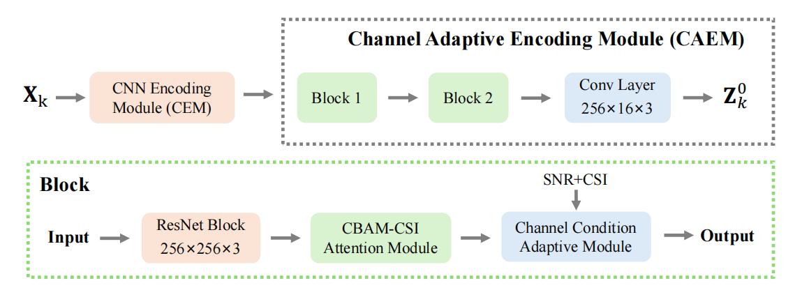
Figure 2: The structure of the semantic encoder.

The semantic decoder denoises the received semantic information and reconstructs the source image by exploiting the multi-head self-attention (MHSA) mechanism. The network structure of the semantic decoder is shown in Fig. 3, where $CADM$ comprises one MHSA module, one convolutional layer, two channel condition adaptive modules, and two ResNet blocks, and $CDM$ comprises two transposed convolutional layers and one convolutional layer, which are configured as $256\times 128\times 3$, $128\times 64\times 3$ , and $64\times 3\times 5$. Overall, the semantic decoder functions as the inverse process of the semantic encoder, progressively reconstructing the source image.

Next, we will introduce the CBAM-CSI module, the channel condition adaptation module in the semantic encoder, and the MHSA module in the semantic decoder in detail.

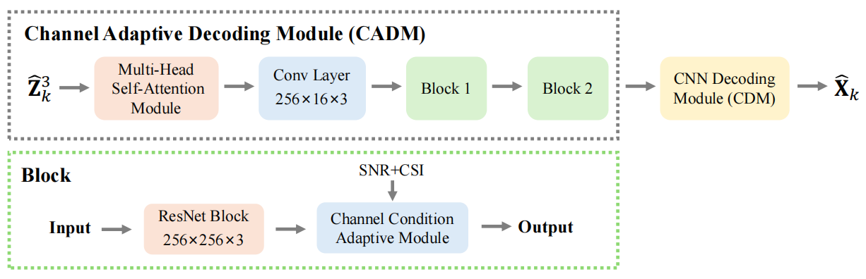
Figure 3: The structure of the semantic decoder.

III-A1 CBAM-CSI Attention Module

The CBAM-CSI attention module includes a channel attention module followed by a spatial attention module, with the feature maps, the estimated CSI, and the estimated channel SNR as inputs.

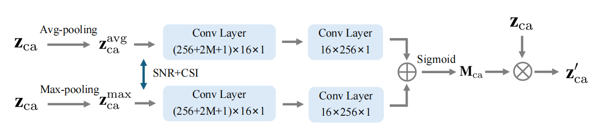
Figure 4: The structure of the channel attention module.

The structure of the channel attention module is shown in Fig. 4. The channel attention module consists of two paths, each containing two $1\times 1$ convolutional layers. These two paths share the same weights and are denoted by $CL(\cdot)$. Denote the input feature maps to this module by $\textbf{z}_{\mathrm{ca}}$. We perform average pooling and max pooling over each feature map of $\textbf{z}_{\mathrm{ca}}$ to obtain $\textbf{z}_{\mathrm{ca}}^{\mathrm{avg}}$ and $\textbf{z}_{\mathrm{ca}}^{\mathrm{max}}$, respectively. Next, $\textbf{z}_{\mathrm{ca}}^{\mathrm{avg}}$ and $\textbf{z}_{\mathrm{ca}}^{\mathrm{max}}$ are concatenated with $\hat{\textbf{{h}}}_{k}$ and $\hat{\mathrm{SNR}}$ with the two feature maps to obtain $\textbf{z}_{\mathrm{ca}}^{\mathrm{avg}^{\prime}}$ and $\textbf{z}_{\mathrm{ca}}^{\mathrm{max}^{\prime}}$, which are then passed through the two paths and added to obtain the channel attention map $\textbf{M}_{\mathrm{ca}}$, denoted by

$$\textbf{M}_{\mathrm{ca}}=\sigma\left(CL\left({\textbf{z}_{\mathrm{ca}}^{\mathrm{avg}^{\prime}}}\right)+CL\left({\textbf{z}_{\mathrm{ca}}^{\mathrm{max}^{\prime}}}\right)\right),$$ (13)

where $\sigma$ represents the sigmoid function. After obtaining $\textbf{M}_{\mathrm{ca}}$, $\textbf{z}_{\mathrm{ca}}$ is multiplied by $\textbf{M}_{\mathrm{ca}}$ to obtain the weighted feature maps $\textbf{z}_{\mathrm{ca}}^{\prime}$. The channel attention module learns to allocate greater weights to the more important channels.

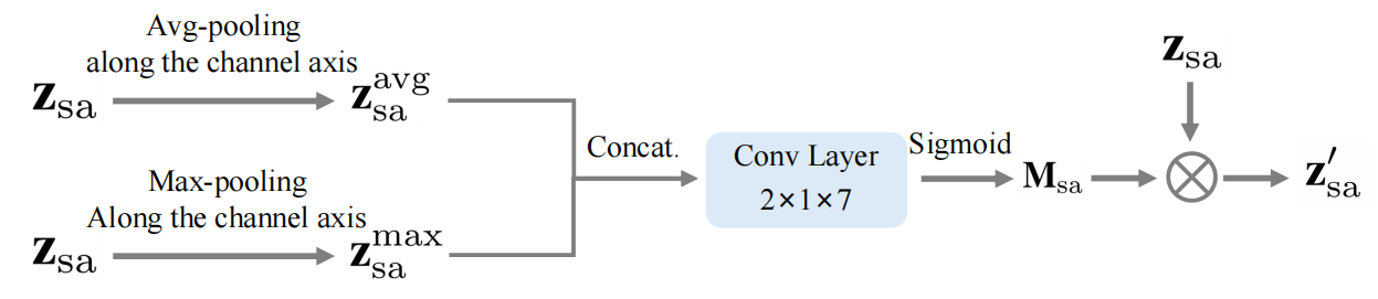
Figure 5: The structure of the spatial attention module.

The structure of the spatial attention module is shown in Fig. 5. Following the channel attention module, the weighted channel maps $\textbf{z}_{\mathrm{ca}}^{\prime}$ are input to the spatial attention module, i.e., $\textbf{z}_{\mathrm{sa}}=\textbf{z}_{\mathrm{ca}}^{\prime}$. Denote the dimensions of $\textbf{z}_{\mathrm{sa}}$ as $C_{\mathrm{sa}}\times H_{\mathrm{sa}}\times W_{\mathrm{sa}}$. We first perform average pooling and max pooling operations on $\textbf{z}_{\mathrm{sa}}$ along the channel axis to obtain two feature maps with dimensions $1\times H_{\mathrm{sa}}\times W_{\mathrm{sa}}$, denoted as $\textbf{z}_{\mathrm{sa}}^{\mathrm{avg}}$ and $\textbf{z}_{\mathrm{sa}}^{\mathrm{max}}$, respectively. These are then concatenated to obtain $\textbf{z}_{\mathrm{sa}}^{\mathrm{concat}}$. Subsequently, $\textbf{z}_{\mathrm{sa}}^{\mathrm{concat}}$ passes through a convolutional layer and a sigmoid function to generate the spatial attention map $\textbf{M}_{\mathrm{sa}}$, defined as

$$\textbf{M}_{\mathrm{sa}}=\sigma\left({Conv}_{7\times 7}\left(Concat\left(\textbf{z}_{\mathrm{sa}}^{\mathrm{avg}},\textbf{z}_{\mathrm{sa}}^{\mathrm{max}}\right)\right)\right),$$ (14)

where ${Conv}_{7\times 7}$ represents a convolution layer with a filter size of $7\times 7$. Finally, the output of the spatial attention module is $\textbf{z}_{\mathrm{sa}}$ weighted by $\textbf{M}_{\mathrm{sa}}$, i.e., $\textbf{z}_{\mathrm{sa}}^{{}^{\prime}}=\textbf{z}_{\mathrm{sa}}\textbf{M}_{\mathrm{sa}}$. The spatial attention module learns to allocate greater weights to the more important elements within each feature map.

III-A2 Channel Condition Adaptive Module

The structure of the channel condition adaptive module is shown in Fig. 6.

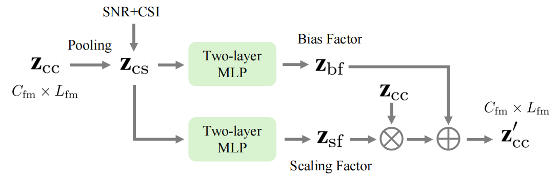
Figure 6: The structure of the channel condition adaptive module.

The input $\textbf{z}_{\mathrm{cc}}$, which initially has dimensions of $C_{\mathrm{fm}}\times L_{\mathrm{fm}}$, is first average pooled, resulting in a dimension of $C_{\mathrm{fm}}\times 1$. Here, $C_{\mathrm{fm}}$ is the number of feature maps and $L_{\mathrm{fm}}$ is the length of each feature map. It is then concatenated with the estimated CSI and channel SNR, denoted as $\textbf{z}_{\mathrm{cs}}$, which has a dimension of $(C_{\mathrm{fm}}+2M+1)\times 1$. Subsequently, $\textbf{z}_{\mathrm{cs}}$ is fed into two different multi-layer perceptrons (MLPs) to obtain a scaling factor $\textbf{z}_{\mathrm{bf}}$ and a bias factor $\textbf{z}_{\mathrm{sf}}$, respectively. Finally, $\textbf{z}_{\mathrm{cc}}$ is multiplied by $\textbf{z}_{\mathrm{bf}}$ and added with $\textbf{z}_{\mathrm{cc}}$ as the final output of the channel condition adaptive module, denoted by $\textbf{z}^{\prime}_{\mathrm{cc}}=\textbf{z}_{\mathrm{cc}}\textbf{z}_{\mathrm{bf}}+\textbf{z}_{\mathrm{cc}}$. By incorporating the estimated CSI and channel SNR into this module, the proposed system can adapt effectively to various channel conditions.

III-A3 Multi-Head Self-Attention Module

The MHSA module consists of multiple self-attention modules running in parallel. The structure of a self-attention module [44] is shown in Fig. 7, includes three learnable weight matrices, $\textbf{W}_{Q}$, $\textbf{W}_{K}$, and $\textbf{W}_{V}$.

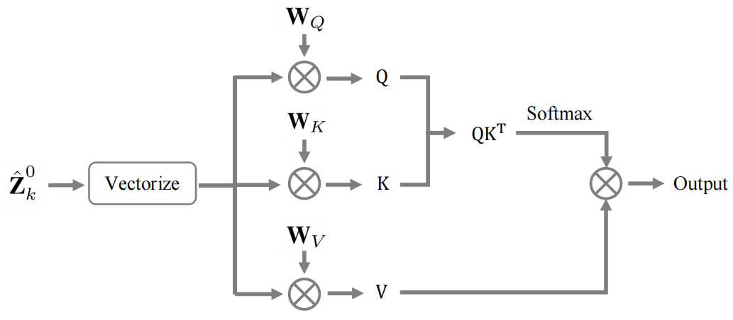
Figure 7: The structure of the self-attention module.

$\hat{\textbf{Z}}_{k}^{0}$ is input to each attention module, where it is first vectorized and then multiplied by these three learnable weight matrices:

$$\textbf{Q}=\textbf{W}_{Q}\cdot\hat{\textbf{Z}}_{k}^{0},~\textbf{K}=\textbf{W}_{K}\cdot\hat{\textbf{Z}}_{k}^{0},~\textbf{V}=\textbf{W}_{V}\cdot\hat{\textbf{Z}}_{k}^{0}.$$ (15)

The output of the self-attention module can be derived as

$$Attention\left(\hat{\textbf{Z}}_{k}^{0}\right)=softmax\left(\frac{\textbf{Q}\textbf{K}^{T}}{\sqrt{d}}\right)\textbf{V},$$ (16)

where $softmax\left(\frac{\textbf{Q}\textbf{K}^{T}}{\sqrt{d}}\right)$ represents the importance weight matrix, V is the value matrix to be scaled, and $d$ denotes the dimension of Q and K. In the MHSA module, $\hat{\textbf{Z}}_{k}^{0}$ is fed into several self-attention modules in parallel, and their outputs are then summed. To mitigate the issue of gradient vanishing, a residual connection is also incorporated into the final output. This MHSA module enables the semantic decoder to denoise semantic information by leveraging the self-attention mechanism to capture spatial relationships among elements in the feature maps.

III-B Feature Map Selection and Pruning Module

The feature map selection and pruning module selects the activated feature maps and prunes each of them to achieve feature map compression.

III-B1 Feature Map Selection Module

The structure of the feature map selection module is shown in Fig. 8.

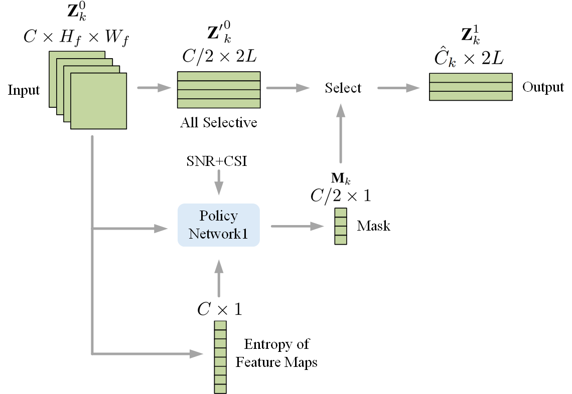
Figure 8: The structure of the feature map selection module.

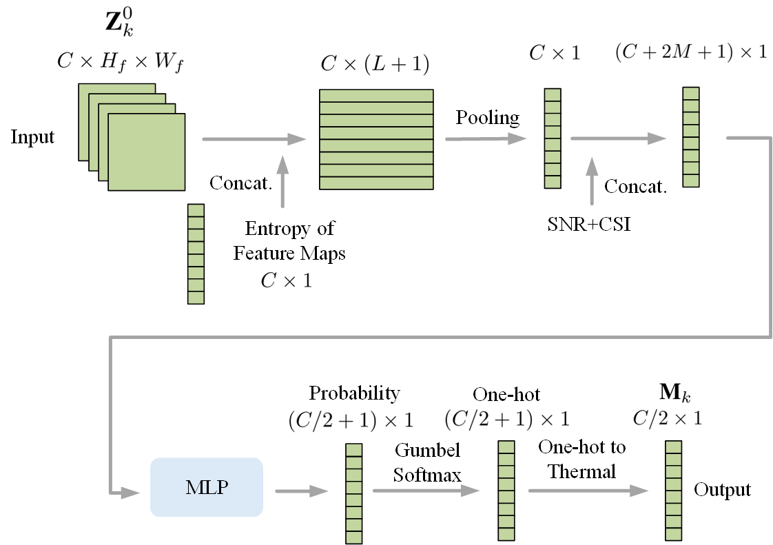
Figure 9: The structure of the policy network $P_{k,1}$.

For the $k$-th user, the input to its feature selection module is denoted by $\textbf{Z}_{k}^{0}$, which has dimensions of $C\times H_{f}\times W_{f}$, where $C$ represents the number of feature maps and $H_{f}$ and $W_{f}$ denotes the height and width of each feature map. The entropy of each feature map $\textbf{Z}_{k,i}^{0}$, denoted as $H(\textbf{Z}_{k,i}^{0})$, is computed using the 2D entropy method proposed in [45]. Specifically, in a feature map, the gray value $m$ of a pixel and the mean gray value $n$ of its neighborhood are used to construct a joint probability distribution $P_{m,n}$, given as

$$P_{m,n}=\frac{q(m,n)}{H_{f}*W_{f}},$$ (17)

where $q(m,n)$ represents the occurrence counts of the pair $(m,n)$ in the feature map. The entropy $H(\textbf{Z}_{k,i}^{0})$ is then computed as

$$H(\textbf{Z}_{k,i}^{0})=-\sum_{m,n}P_{m,n}\log_{2}P_{m,n}.$$ (18)

This computation captures both the intensity distribution and the spatial characteristics of each feature map, enabling a comprehensive quantification of its information richness. Then, in order to increase the difference between the entropy values of different feature maps, we apply the softmax function,

$$H^{\prime}\left(\textbf{Z}_{k,i}^{0}\right)=\frac{e^{H(\textbf{Z}_{k,i}^{0})}}{\sum\limits_{i=1}^{2C}e^{H(\textbf{Z}_{k,i}^{0})}},$$ (19)

to normalize $H(\textbf{Z}_{k,i}^{0})$. The overall entropy vector $H^{\prime}(\textbf{Z}_{k}^{0})$ is obtained by concatenating all $H^{\prime}(\textbf{Z}_{k,i}^{0})$. To create complex transmission symbols, one half of the feature maps is used as the real part, and the other half as the imaginary part. Consequently, every two feature maps in $\textbf{Z}_{k}^{0}$ are concatenated and vectorized to form ${\textbf{Z}^{\prime}}_{k}^{0}\in\mathbb{R}^{C/2\times 2L}$, where $L=H_{f}\cdot W_{f}$. We then determine which of these $C/2$ feature maps to select, rather than considering only half of the feature maps as done in the previous method [32]. Specifically, $\textbf{Z}_{k}^{0}$, $H^{\prime}(\textbf{Z}_{k}^{0})$, the estimated CSI and channel SNR are fed into the policy network $P_{k,1}$, which outputs a binary mask $\textbf{M}_{k}\in\left\{0,1\right\}^{C/2\times 1}$ indicating which feature maps should be sent.

The structure of the proposed policy network $P_{k,1}$, $k=1,...,K$, inspired by [32], is illustrated in Fig. 9. We first vectorize each feature map in $\textbf{Z}_{k}^{0}$, which is then concatenated with $H^{\prime}(\textbf{Z}_{k}^{0})$ to form an information matrix of dimension $C\times(L+1)$. Next, we average each row of this matrix and concatenate the resulting vector with the estimated channel SNR and CSI $\hat{\textbf{h}}_{k}$, generating a $(C+2M+1)\times 1$ vector. Here, the CSI vector contains $2M$ elements because the real and imagenery parts of each CSI value are treated as two separate elements. This vector is then fed into a two-layer MLP to produce a probability vector of length $C/2+1$，where the first $C/2$ elements represent the probabilities of selecting the $C/2$ complex feature maps, and the last element represents the probability of not selecting any feature map. Note that directly sampling the selection vector from the probability vector results in non-differentiability problem during training. Therefore, we utilize Gumbel-Softmax technique [46] to sample a one-hot vector, which is then transformed into the selection vector $\textbf{M}_{k}$. Specifically, $\textbf{M}_{k}$ is obtained by setting all subsequent elements, starting from the position of the element with a value of $1$ in the one-hot vector, to 1, a process referred to as thermometer coding. Note that if the last element in the one-hot vector is $1$, then $\textbf{M}_{k}$ is a vector of zeros.

$\textbf{M}_{k}$ is then used to select the feature maps in ${\textbf{Z}^{\prime}}_{k}^{0}$, where each “1” in $\textbf{M}_{k}$ indicates selecting the corresponding feature map, and “0” indicates discarding the corresponding feature map. We denote the total number of selected feature maps as $\hat{C_{k}}={\sum\limits_{i=1}^{C/2}M_{k(i)}}$. The transmitter then only sends the selected feature maps, while the receiver replaces the discarded feature maps with zeros.

III-B2 Feature Map Pruning Module

The structure of the feature map pruning module is illustrated in Fig. 10. In this module, the policy network $P_{k,2}$ is employed to determine the pruning ratio of the selected feature maps. The policy network takes $\textbf{Z}_{k}^{1}$ as its input. The detailed structure of the policy network $P_{k,2}$ is shown in Fig. 11.

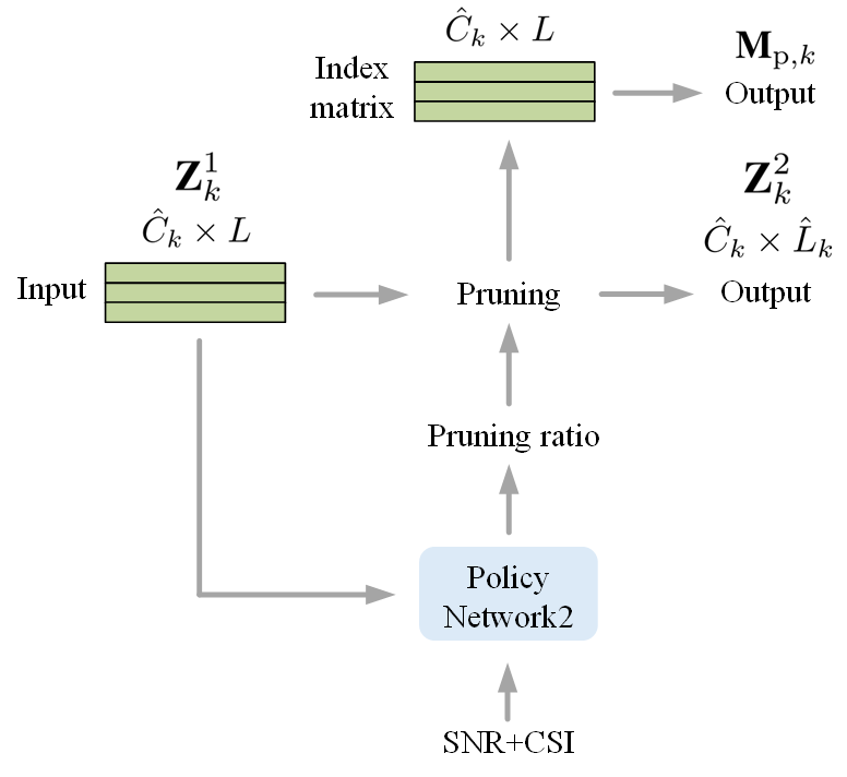
Figure 10: The structure of the feature map pruning module.

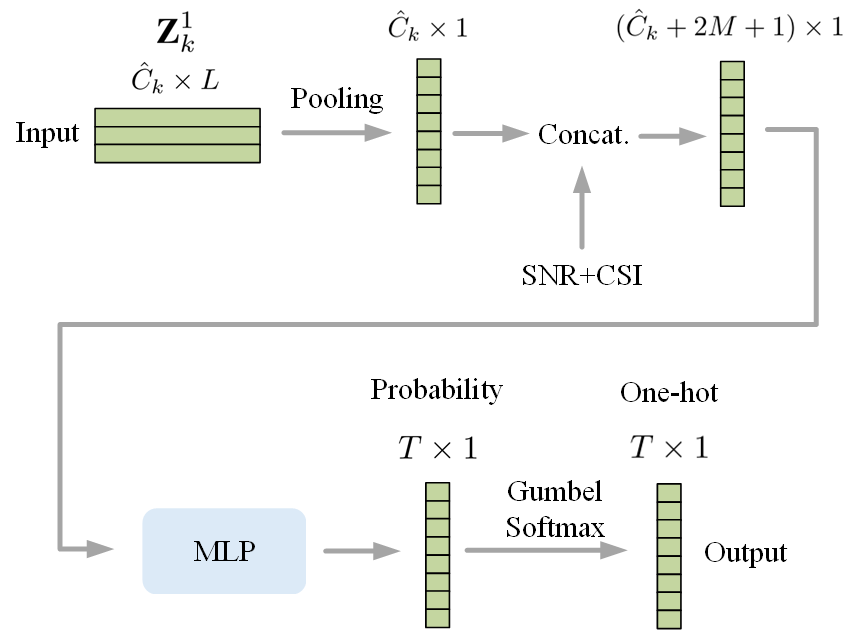
Figure 11: The structure of the policy network $P_{k,2}$.

We first apply average pooling to each row of $\textbf{Z}_{k}^{1}$ and concatenate the resulting vector with the estimated channel SNR and CSI $\hat{\textbf{h}}_{k}$. The concatenated vector is then passed through a MLP, which consists of two fully connected layers followed by a softmax function. This MLP then output a probability vector of length $T$, where $T$ is the number of predefined pruning ratios. In this paper, we set the length $T$ to 5 and define the corresponding pruning ratios as $a\in\left\{0,0.2,0.3,0.4,0.5\right\}$. By applying the Gumbel-Softmax trick to this vector, we generate a one-hot vector $\textbf{V}_{k}$. We prune $\textbf{Z}_{k}^{1}$ with the pruning ratio given by $\textbf{V}_{k}$ to obtain pruned feature maps $\textbf{Z}_{k}^{2}$. The dimension of $\textbf{Z}_{k}^{2}$ is denoted by $\hat{C}_{k}\times\hat{L}_{k}$. Specifically, inspired by the commonly used $l$1-norm based pruning rule[47], we regard pixels within each activated feature map with smaller $l$1-norm (i.e., pixels with smaller absolute numerical values) as less important. We remove pixels with smaller $l$1-norm in each activated feature map according to the pruning ratio. It is essential for the receiver to know the positions of the pruned pixels to reconstruct the original feature maps. Therefore, we also transmit the pruning index matrix $\textbf{M}_{\mathrm{p},k}\in\left\{0,1\right\}^{\hat{C}_{k}\times 2L}$, where a value of $1$ indicates that the pixel at the corresponding position has been pruned. Using the received $\textbf{M}_{\mathrm{p},k}$, the receiver can zero-pad the pruned pixels to restore the feature maps.

III-C Channel Encoder and Decoder

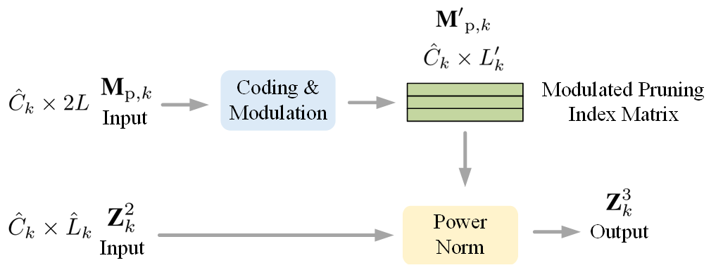
Figure 12: The structure of the channel encoder.

The structure of the channel encoder is illustrated in Fig. 12. This channel encoder at the $k$-th user performs traditional channel coding and modulation on $\textbf{M}_{\mathrm{p},k}$ to transmit the pruning indices. We denote the number of symbols required for transmitting each pruning index vector in $\textbf{M}_{\mathrm{p},k}$ by $L_{k}^{\prime}$, which depends on the employed channel coding and modulation scheme. The dimension of the modulated pruning index matrix ${\textbf{M}^{\prime}}_{\mathrm{p},k}$ is then $\hat{C}_{k}\times L_{k}^{\prime}$. The channel encoder then performs power normalization on the pruned feature maps $\textbf{Z}_{k}^{2}$ and ${\textbf{M}^{\prime}}_{\mathrm{p},k}$:

$$\textbf{Z}_{k}^{3}=PN(\textbf{Z}_{k}^{2},{\textbf{M}^{\prime}}_{\mathrm{p},k}),s.t.\frac{1}{L_{\mathrm{z}}}\mathbb{E}\left[\left\|\textbf{Z}_{k}^{3}\right\|_{2}^{2}\right]\leq P,$$ (20)

where $\textbf{Z}_{k}^{3}~\epsilon~\mathbb{C}^{L_{\mathrm{z}}\times 1}$, $L_{\mathrm{z}}=\hat{C}_{k}\times\left(\frac{\hat{L}_{k}+L_{k}^{\prime}}{2}\right)$ and $P$ is the power constraint. The transmitted signals of all users are denoted by $\textbf{Z}=\left[\textbf{Z}_{1}^{3},\textbf{Z}_{2}^{3},\cdots,\textbf{Z}_{K}^{3}\right]\in\mathbb{C}^{L_{z}\times K}$, which are sent over the MU-MIMO Rayleigh fading channels.

The receiver then receives $\textbf{Y}^{T}=\left[\hat{\textbf{Z}}_{1},\hat{\textbf{Z}}_{2},\cdots,\hat{\textbf{Z}}_{M}\right]\in\mathbb{C}^{L_{z}\times M}$, which is processed by the L-MMSE signal detector to recover the transmitted signals ${\hat{\textbf{Z}}}^{T}=\left[\hat{\textbf{Z}}_{1}^{4},\hat{\textbf{Z}}_{2}^{4},\cdots,\hat{\textbf{Z}}_{K}^{4}\right]\in\mathbb{C}^{L_{z}\times K}$. Finally, $\hat{\textbf{Z}}_{k}^{4}$ is fed into the $k$-th channel decoder, for $k=1,\ldots,K$.

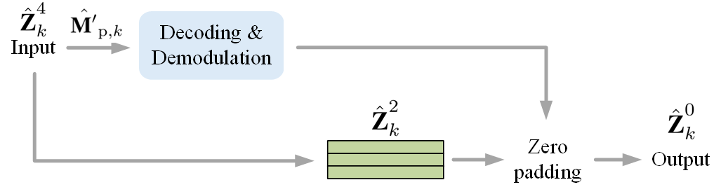
Figure 13: The structure of the channel decoder.

The structure of the channel decoder is shown in Fig. 13. $\hat{\textbf{Z}}_{k}^{4}$ consists of two parts, namely the recovered transmitted signal and the modulated pruning index matrix, denoted by $\hat{\textbf{Z}}_{k}^{2}$ and $\hat{{\textbf{M}’}}_{\mathrm{p},k}$, respectively. $\hat{{\textbf{M}’}}_{\mathrm{p},k}$ is then demodulated and decoded through the reverse operation of the channel encoder. Next, we zero-pad $\hat{\textbf{Z}}_{k}^{2}$ based on the demodulated pruning index matrix to recover the structure of the selected feature maps. Subsequently, the feature maps that were not selected by the transmitter are replaced by zero matrices. Finally all the feature maps are converted from complex values back to real values, resulting in $\hat{\textbf{Z}}_{k}^{0}$, which is the output of the channel decoder.

III-D Loss Function

To train our proposed SemCom system, we incorporate three terms into our loss function $\mathcal{L}$, which is defined as

$$\begin{split}\mathcal{L}=&\mathbb{E}\Bigg{[}\left\|{\textbf{X}_{k}-{\hat{\textbf{X}}}_{k}}\right\|_{2}^{2}+\\ &\alpha\frac{\hat{L}_{k}+L_{k}^{\prime}}{2L}{\sum_{i=1}^{C/2}M_{k(i)}}-\beta\frac{1}{C}{\sum_{i=1}^{C}e^{H(\textbf{Z}_{k(i)}^{0})}}\Bigg{]},\end{split}$$ (21)

where the expectation is taken over the entire training set across all users. The first term is the mean square error (MSE) between source images and reconstructed images, ensuring image reconstruction performance. The second term is the product of the length ratio and the number of the activated feature maps. This term represents wireless channel usage and helps reduce the necessary channel bandwidth. The third term indicates the average processed entropy of $\textbf{Z}_{k}^{0}$. During training, we maximize the average entropy of the feature maps to increase the average amount of information carried by each transmitted symbol. In order to increase the difference between the values, we instead use the exponential of the entropy of each feature map. This term is calculated by taking the average value of the processed entropy of all $C$ feature maps. We use two hyperparameters $\alpha$ and $\beta$ to govern the tradeoff between these three terms.

III-E Training Strategy

We employ the Adam optimizer [48] to train our model, where its weight decay is set to $5\times 10^{-4}$. Specifically, we first train the entire model for 150 epochs with a learning rate of $1\times 10^{-3}$. Subsequently, we decrease the learning rate to $1\times 10^{-4}$ and continue training for 100 epochs. Afterwards, we proceed to the fine-tuning phase, where the learning rate becomes $1\times 10^{-5}$. During this phase, we first freeze $CEM$ and $P_{2}$, and train the model for 150 epochs. Then, we freeze $CAEM$ and $P_{1}$, and train the model for 100 epochs.

IV Simulation Results

In this section, we comprehensively evaluate various aspects of our proposed system. We begin by presenting the experimental settings. Next, we analyze the learned image transmission strategy of our system. We then compare the performance of the proposed SemCom system with the benchmarks. Following this, we assess the robustness of our system to imperfect CSI and inter-user interference [49]. Finally, we conduct ablation studies to verify the effectiveness of each module within the proposed system.

IV-A Experimental Settings

IV-A1 Dataset

We use the CIFAR-10 dataset [50], which consists of 50,000 training images and 10,000 testing images, all of which are $32\times 32$ RGB images.

IV-A2 Experimental Settings

The training batch size is set to 512. During training, the channel SNR is uniformly sampled between 0 dB and 25 dB. The initial value of the temperature parameter, $\tau$, for the Gumbel-Softmax in the policy networks is set to 5, with an exponential decay rate of 0.01. The hyperparameter $\alpha$ takes two distinct values: $2\times 10^{-4}$ and $3\times 10^{-4}$. The value of $\beta$ is set to $1\times 10^{-5}$.

The number of filters in the last layer of the semantic encoder is $C=16$, and the length of the corresponding feature map is $L=64$. Hence, the final complex latent feature ${\textbf{Z}^{\prime}}_{k}^{0}$ for the policy networks to prune has a dimension of $\frac{C}{2}\times 2L=8\times 128$. The feature map selection vector $\textbf{M}_{k}$ is thus only 8 bits long. Note that this transmission cost is neglected when calculating the compression ratio. The binary vectors used to represent the indices of pruned elements in each pruned feature map consist of $128$ bits. We apply $\frac{3}{4}$ low-density parity-check (LDPC) codes to channel-code the pruning index matrix $\textbf{M}_{\mathrm{p},k}$, followed by modulation using 64 quadrature amplitude modulation (64-QAM) to generate $\textbf{M}^{\prime}_{\mathrm{p},k}$. We have the length of each row in $\textbf{M}^{\prime}_{\mathrm{p},k}$ $L_{k}^{\prime}=\left\lceil\frac{2L\times\frac{4}{3}}{6}\right\rceil$ if elements in feature maps are pruned; otherwise, $L_{k}^{\prime}=0$. For the $k$-th user, its CPP is calculated as $\mathrm{CPP}_{k}=\frac{\hat{C_{k}}\left(\hat{L}_{k}+L_{k}^{\prime}\right)}{2HW}$.

We consider both perfect CSI and imperfect CSI in the experimental studies. For imperfect CSI, we have $\hat{\textbf{H}}=\textbf{H}+\mathrm{\Delta}\textbf{H}$, where H denotes the perfect CSI and $\mathrm{\Delta}\textbf{H}\sim\mathcal{C}\mathcal{N}\left(0,\sigma_{e}^{2}\right)$ represents the channel estimation error. We set $\sigma_{e}^{2}=\sigma_{n}^{2}$. Results presented are based on perfect CSI unless explicitly stated otherwise.

IV-A3 The Benchmarks

We use two benchmarks for comparison. The first benchmark employs the standard deep joint source and channel coding (deep JSCC) architecture [51], which we extend to the multi-user case and train with a channel SNR of 25dB, referred to as deep JSCC. We use the encoder-decoder pair proposed in [51] as the encoder-decoder pair for each user. We set two fixed CPPs, i.e., 0.328 and 0.289. The second benchmark employs separated source and channel coding method. The source image is compressed using the BPG encoder, which is an image compression method that outperforms JPEG in terms of compression quality and compression ratio. For the channel coding method, we use LDPC. To modulate the coded bits, we use 4-QAM. During the simulation, our BPG encoder employs the JCT-VC HEVC codec [52] as the compression method. The color precision of each pixel is set to 8. The quantizer parameter Q is directly related to the compression rate and controls the image compression quality. Increasing Q leads to higher compression rates but lower CPP. For instance, when the value of Q is 45, it corresponds to a CPP of 0.322. The LDPC codes adhere to the DVB-S.2 standard with a coding rate of 1/2. We name this benchmark BPG+LDPC+4QAM.

IV-B Evaluation of adaptive rate control

TABLE I: The transmission rate under different channel SNR values with $\alpha=2\times 10^{-4}$.

SNR (dB)	Number of selected feature maps	Feature map length ratio(%)	Transmission rate (CPP)	PSNR (dB)
25	5.65	59	0.288	32.95
20	5.70	62	0.301	32.88
15	5.81	68	0.329	32.75
10	5.90	77	0.367	30.83
5	5.96	100	0.372	28.01
0	5.16	100	0.322	24.44

TABLE II: The transmission rate under different channel SNR values with $\alpha=3\times 10^{-4}$.

SNR (dB)	Number of selected feature maps	Feature map length ratio(%)	Transmission rate (CPP)	PSNR (dB)
25	4.73	56	0.232	31.27
20	4.81	59	0.245	31.27
15	4.85	72	0.287	31.29
10	4.93	79	0.313	30.05
5	4.99	100	0.311	27.35
0	4.66	100	0.291	23.91

We analyze the learned adaptive rate control under different channel conditions, which are determined by the selected number of feature maps and pruning ratios through our proposed entropy-and-channel adaptive rate control mechanism. Our system is trained under varing channel SNR from 0 dB to 25 dB, using the loss function given in (21), with $\beta=1\times 10^{-5}$, and two different $\alpha$ values, i.e., $\alpha=2\times 10^{-4}$ and $\alpha=3\times 10^{-4}$, respectively. The results, presented in Table I and Table II, are averaged over the entire testing dataset across all users. The feature map length ratio represents the percentage of unpruned pixels in the activated feature maps.

We can observe from Table I and Table II that the proposed method dynamically adjusts the transmission rate based on the channel SNR, resulting in different PSNR performances. We also note that increasing $\alpha$ reduces the CPP, meaning fewer symbols are transmitted, albeit at the cost of a slight PSNR decrease. This trade-off occurs because $\alpha$ prioritizes minimizing channel resource usage, leading the model to reduce CPP as $\alpha$ increases. From Table I and Table II, when the SNR is very low (0–5 dB), the model increases the CPP by selecting more feature maps as the SNR increases. This adjustment compensates for the substantial errors caused by channel fading at low SNRs. Conversely, when the SNR is high (10–25 dB), the model prunes the feature maps. As SNR improves, fewer feature maps are selected, and even fewer pixels within these maps are retained, resulting in lower CPP. This adaptive behavior ensures reduced transmission overhead under favorable channel conditions while maintaining high PSNR performance.

Overall, the results demonstrate that our feature map selection and pruning module effectively balances the trade-off between transmission efficiency and image quality by dynamically selecting important feature maps and removing less significant pixels based on the channel conditions. This enables our system to improve rate-distortion performance.

IV-C Performance Comparison with Benchmarks

We compare the image transmission performance of our proposed system with the benchmarks on the CIFAR-10 dataset in terms of reconstruction quality and transmission rate, as shown in Fig. 14. For a fair comparison, we tune the quantization parameter Q of BPG+LDPC+4QAM to match the CPPs of our proposed system at various SNR levels. Meanwhile, the CPP of Deep JSCC is fixed at 0.328 (Fig. 14a) and 0.289 (Fig. 14b). Our proposed system demonstrates excellent performance across all SNRs using a single model, highlighting its superior adaptability compared to the benchmarks. Our system outperforms BPG+LDPC+4QAM across the entire SNR range (0–25 dB), achieving significant improvements in PSNR with similar CPPs. Specifically, when $\alpha=2\times 10^{-4}$, our proposed system achieves more than 3.5 dB PSNR improvement compared to BPG+LDPC+4QAM at high SNRs (20–25 dB). When $\alpha=3\times 10^{-4}$, the improvement exceeds 2.5 dB under comparable conditions. At low SNRs, BPG+LDPC+4QAM exhibits substantial performance degradation, whereas our proposed system maintains strong performance due to its robust feature map selection and pruning strategy. Additionally, our proposed system achieves approximately 0.4-0.8 dB higher PSNR compared to Deep JSCC with similar CPPs, benefiting from its ability to dynamically select and prune feature maps based on channel conditions and entropy. This adaptability also ensures that our system suffers less performance degradation than Deep JSCC as SNR decreases.

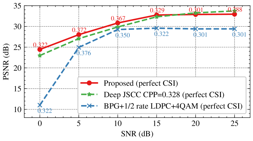
(a) $\alpha=2\times 10^{-4}$

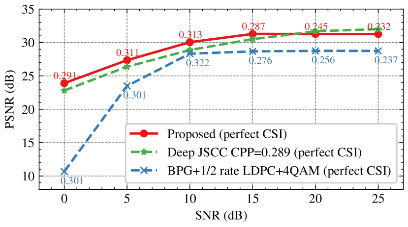
(b) $\alpha=3\times 10^{-4}$

Figure 14: Performance comparison between our proposed system and the benchmarks. The CPPs of each model are labeled next to the curve, and the CPP of Deep JSCC is fixed.

IV-D Impact of Imperfect CSI

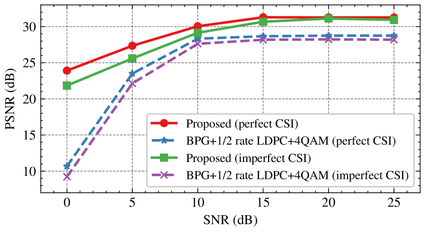
Figure 15: Performance evaluation of the proposed method and BPG+LDPC+4QAM w.r.t. perfect CSI and imperfect CSI. For the proposed system, we set $\alpha=3\times 10^{-4}$.

We analyze the performance of our proposed system and BPG+LDPC+4QAM w.r.t perfect CSI and imperfect CSI, as shown in Fig. 15. The corresponding CPPs are shown in Table. III.

TABLE III: The CPPs under different SNR values in Fig. 15.

SNR(dB)	0	5	10	15	20	25
Proposed (perfect CSI)	0.291	0.311	0.313	0.287	0.245	0.232
BPG+LDPC+4QAM (perfect CSI)	0.301	0.301	0.322	0.276	0.256	0.237
Proposed (imperfect CSI)	0.312	0.312	0.322	0.318	0.271	0.260
BPG+LDPC+4QAM (imperfect CSI)	0.301	0.301	0.322	0.322	0.276	0.256

From the results, it is observed that imperfect CSI leads to a degradation in PSNR performance and an increase in CPP. At low SNRs, the degradation in PSNR caused by imperfect CSI is more significant, as the channel estimation is less accurate under poor channel conditions. However, at high SNRs, the performance degradation is relatively minor due to improved channel estimation accuracy. Despite the degradation caused by imperfect CSI, our proposed system still outperforms BPG+LDPC+4QAM under perfect CSI across all SNRs, as well as BPG+LDPC+4QAM under imperfect CSI. This highlights the robustness of our proposed system to imperfect CSI conditions. We note that the proposed system exhibits slightly increased CPP values to compensate for imperfect CSI, resulting in smaller performance degradation, especially in the high SNR region. This adaptability makes the proposed method highly suitable for real-world scenarios where channel state information may not always be accurate.

IV-E Different Number of Users

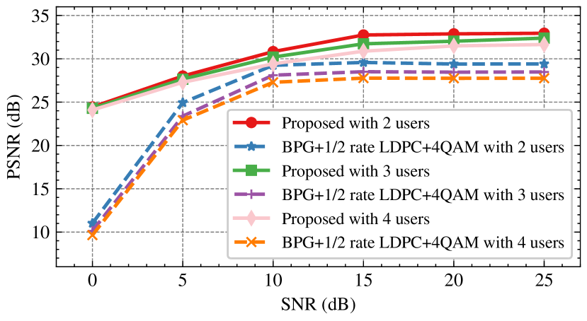
Figure 16: Performance evaluation of our proposed system and BPG+LDPC+4QAM under different number of users. For the proposed system, we set $\alpha=2\times 10^{-4}$.

We evaluate the performance of our proposed system and BPG+LDPC+4QAM under different number of users, as shown in Fig. 16. The corresponding CPPs are shown in Table. V.

TABLE IV: The CPPs under different SNR values (perfect CSI) in Fig. 16.

SNR(dB)	0	5	10	15	20	25
Proposed (2 Users)	0.322	0.372	0.367	0.329	0.301	0.288
BPG+LDPC+4QAM (2 Users)	0.322	0.376	0.350	0.322	0.301	0.301
Proposed (3 Users)	0.312	0.313	0.294	0.281	0.264	0.265
BPG+LDPC+4QAM (3 Users)	0.301	0.301	0.301	0.276	0.276	0.276
Proposed (4 Users)	0.281	0.292	0.262	0.265	0.258	0.251
BPG+LDPC+4QAM (4 Users)	0.276	0.276	0.256	0.256	0.256	0.256

From the results, we observe that both the CPP and PSNR values of the proposed method decrease with an increasing number of users, which may be due to inter-user interference. However, the rate-distortion performance is stable, highlighting the robustness of our proposed system. For BPG+LDPC+4QAM, a similar trend is observed, where both the PSNR and CPP degrade as the number of users increases. However, the degradation in BPG+LDPC+4QAM is more pronounced compared to our proposed system. It can be easily observed that our system consistently outperforms BPG+LDPC+4QAM with different number of users. Notably, even with four users, our proposed system surpasses the performance of BPG+LDPC+4QAM with only two users. This result demonstrates the superior robustness of our proposed system to inter-user interference and its ability to maintain high rate-distortion performance under challenging conditions.

IV-F Ablation Studies

In this section, we analyze the performance of the proposed system under different configurations to demonstrate the effectiveness of its design.

IV-F1 Entropy-aware and/or Attention Mechanisms

We evaluate the proposed system without the entropy-aware mechanism (abbreviated as entropy), and then without both the entropy-aware mechanism and the attention mechanisms, as shown in Table V and Table VI. We observe that the removal of attention mechanisms results in a significant decrease in PSNR performance across all SNRs. For instance, when $\alpha=3\times 10^{-4}$ and SNR = 25 dB, the PSNR decreases by 0.68 dB compared to the system with attention mechanisms. This trend holds across all other SNRs, where the system with attention mechanisms consistently demonstrates better rate-distortion performance. The entropy-aware mechanism improves PSNR by 0.09–0.20 dB across all SNRs. At low SNRs (e.g., 0–10 dB), the entropy-aware mechanism achieves the largest PSNR improvements, up to 0.20 dB, suggesting that it is particularly beneficial under poor channel conditions. At higher SNRs, the entropy-aware mechanism also improves the rate-distortion performance, although the improvement is less significant.

TABLE V: The Performance evaluation of the proposed method with and without without the entropy-aware mechanism and the attention mechanisms. Assume perfect CSI feedback and $\alpha=2\times 10^{-4}$.

SNR(dB)	0	5	10	15	20	25
Proposed (PSNR,dB)	24.44	28.01	30.83	32.75	32.88	32.95
Proposed (CPP)	0.322	0.372	0.367	0.329	0.301	0.288
Proposed w/o entropy (PSNR,dB)	24.24($\downarrow 0.20$)	27.83($\downarrow 0.18$)	30.67($\downarrow 0.16$)	32.60($\downarrow 0.15$)	32.76($\downarrow 0.12$)	32.85($\downarrow 0.10$)
Proposed w/o entropy (CPP)	0.325	0.375	0.371	0.331	0.301	0.288
Proposed w/o entropy and attention (PSNR,dB)	23.94($\downarrow 0.50$)	27.42($\downarrow 0.59$)	30.32($\downarrow 0.51$)	31.96($\downarrow 0.79$)	32.59($\downarrow 0.29$)	32.87($\downarrow 0.08$)
Proposed w/o entropy and attention (CPP)	0.309	0.343	0.347	0.342	0.325	0.321

TABLE VI: The Performance evaluation of the proposed method with and without without the entropy-aware mechanism and the attention mechanisms. Assume perfect CSI feedback and $\alpha=3\times 10^{-4}$.

SNR(dB)	0	5	10	15	20	25
Proposed (PSNR,dB)	23.91	27.35	30.05	31.29	31.27	31.27
Proposed (CPP)	0.291	0.311	0.313	0.287	0.245	0.232
Proposed w/o entropy (PSNR,dB)	23.71($\downarrow 0.20$)	27.18($\downarrow 0.17$)	29.91($\downarrow 0.14$)	31.15($\downarrow 0.14$)	31.15($\downarrow 0.12$)	31.18($\downarrow 0.09$)
Proposed w/o entropy (CPP)	0.296	0.314	0.316	0.288	0.245	0.232
Proposed w/o entropy and attention (PSNR,dB)	23.57($\downarrow 0.34$)	26.74($\downarrow 0.61$)	28.73($\downarrow 1.32$)	29.97($\downarrow 1.32$)	30.45($\downarrow 0.82$)	30.59($\downarrow 0.68$)
Proposed w/o entropy and attention (CPP)	0.276	0.280	0.245	0.246	0.236	0.229

IV-F2 CSI Feedback

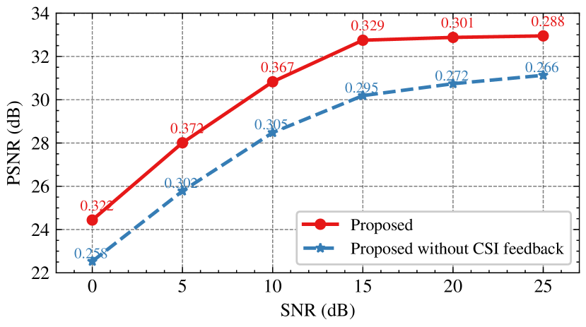
(a) $\alpha=2\times 10^{-4}$

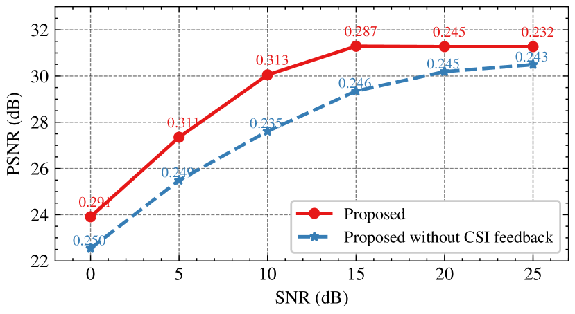
(b) $\alpha=3\times 10^{-4}$

Figure 17: Performance evaluation of our system with and without CSI feedback. The CPPs of each model are labeled next to the curve.

We evaluate the performance of the proposed system with and without CSI feedback to demonstrate its effectiveness, as illustrated in Fig. 17. It can be seen that, without CSI feedback, the system selects a lower CPP, which is not suitable for the channel conditions, resulting in significant degradation in PSNR performance across all SNR levels. For instance, when $\alpha=2\times 10^{-4}$, the PSNR at an SNR of 25 dB decreases by approximately 1.8 dB compared to that with CSI feedback. This substantial drop highlights the critical role of the CSI feedback mechanism in enabling the system to adapt to varying channel conditions. With the CSI feedback mechanism, our proposed system is capable of dynamically learning an optimal transmission strategy based on real-time channel conditions. This ensures optimal rate-distortion performance by selecting an appropriate CPP while maintaining high PSNR values.

IV-F3 Feature Map Pruning Module

We the evaluate the performance of our proposed system without the feature map pruning module (abbreviated as FMPM) to demonstrate its effectiveness, summarized in Table VII. To ensure a fair comparison, we train the model with different $\alpha$ values, which are carefully selected through multiple iterations to ensure that the CPPs of the two systems being compared are similar. As can be seen from Table VII, the PSNR performance of the proposed system with FMPM improves significantly at similar CPPs. Specifically, at $\alpha=2\times 10^{-4}$, the system with FMPM achieves a CPP of 0.288, which is close to that of the system without FMPM at $\alpha=10\times 10^{-4}$ with a CPP of 0.292, but provides a PSNR improvement of 0.66 dB. We recall that when the value of $\alpha$ is smaller, it indicates that more channel resources are available. In such scenarios, the FMPM plays a more significant role by efficiently improving rate-distortion performance. Conversely, as channel resources become scarcer (higher $\alpha$ values), the impact of the FMPM diminishes but remains positive. Overall, the feature map pruning module effectively enhances the PSNR performance of the proposed system, especially under conditions of abundant channel resources.

TABLE VII: Performance evaluation of the proposed method with and without the feature map pruning module (abbreviated as FMPM).

SNR (dB)	Model	Rate (CPP)	PSNR (dB)
25	$\alpha=2\times 10^{-4}$ (w/ FMPM)	0.288	32.95($\uparrow$0.66)
	$\alpha=10\times 10^{-4}$ (w/o FMPM)	0.292	32.29
20	$\alpha=3\times 10^{-4}$ (w/ FMPM)	0.245	31.27($\uparrow$0.22)
	$\alpha=20\times 10^{-4}$ (w/o FMPM)	0.245	31.05

V Conclusion

This paper proposed a novel SemCom system for wireless image transmission that leverages an entropy-and-channel-adaptive mechanism to achieve efficient and robust communication under MU-MIMO fading channels. Unlike traditional methods, the proposed system dynamically adjusts the transmission rate based on the entropy of feature maps, CSI, and SNR. This ensures optimal utilization of communication resources while maintaining high-quality image reconstruction. Specifically, we introduce two policy networks: one to select feature maps for transmission and another to prune elements within the feature maps, thereby reducing transmission overhead without compromising semantic fidelity. Additionally, the proposed method maximizes the entropy during training to enhance the average information carried by each transmitted symbol. Attention mechanisms, including channel attention, spatial attention, and MHSA, enable the system to focus on critical features and effectively reconstruct images, even under noisy conditions. Experimental results demonstrate that the proposed system outperforms BPG+LDPC+4QAM and deep JSCC in terms of rate-distortion performance, transmission rate flexibility, and robustness. Specifically, the system achieves superior performance in challenging scenarios, including low SNR, imperfect CSI, and inter-user interference. These results validate the effectiveness of the entropy-and-channel-adaptive mechanism in dynamic communication environments. Future work will focus on extending this framework to support multimodal data, real-time video transmission, and ultra-dense network scenarios, thereby broadening its applicability to more complex and bandwidth-intensive communication tasks.

References

- [1] W. Chen, Y. Chen, Q. Yang, C. Huang, Q. Wang, and Z. Zhang, “Deep joint source-channel coding for wireless image transmission with entropy-aware adaptive rate control,” in IEEE GLOBECOM, Kuala Lumpur, Malaysia, December 4-8, 2023, pp. 2239–2244.
- [2] X. Luo, H. Chen, and Q. Guo, “Semantic communications: Overview, open issues, and future research directions,” IEEE Wirel. Commun., vol. 29, no. 1, pp. 210–219, Jan. 2022.
- [3] J. Liu, S. Shao, W. Zhang, and H. V. Poor, “An indirect rate-distortion characterization for semantic sources: General model and the case of gaussian observation,” IEEE Trans. Commun., vol. 70, pp. 5946–5959, 2022.
- [4] K. Chi, Q. Yang, Z. Yang, Y. Duan, and Z. Zhang, “Capacity optimizing resource allocation in joint source-channel coding systems with qos constraints,” IEEE Trans. Commun., pp. 1–1, 2024.
- [5] W. Yang, Z. Q. Liew, W. Y. B. Lim, Z. Xiong, D. Niyato, X. Chi, X. Cao, and K. B. Letaief, “Semantic communication meets edge intelligence,” IEEE Wirel. Commun., vol. 29, no. 5, pp. 28–35, Oct. 2022.
- [6] P. Jiang, C. Wen, S. Jin, and G. Y. Li, “Wireless semantic communications for video conferencing,” IEEE J. Sel. Areas Commun., vol. 41, no. 1, pp. 230–244, Nov. 2023.
- [7] G. Zheng, Q. Ni, K. Navaie, H. Pervaiz, and C. C. Zarakovitis, “A distributed learning architecture for semantic communication in autonomous driving networks for task offloading,” IEEE Commun. Mag., vol. 61, no. 11, pp. 64–68, Nov. 2023.
- [8] N. Farsad, M. Rao, and A. Goldsmith, “Deep learning for joint source-channel coding of text,” in Proc. IEEE ICASSP, Calgary, AB, Canada, April 15-20, 2018, pp. 2326–2330.
- [9] H. Xie, Z. Qin, G. Y. Li, and B. Juang, “Deep learning enabled semantic communication systems,” IEEE Trans. Signal Process., vol. 69, pp. 2663–2675, Apr. 2021.
- [10] T. Han, Q. Yang, Z. Shi, S. He, and Z. Zhang, “Semantic-aware speech to text transmission with redundancy removal,” in Proc. IEEE ICC Workshops, Seoul, Korea, May 16-20, 2022, pp. 717–722.
- [11] X. Peng, Z. Qin, D. Huang, X. Tao, J. Lu, G. Liu, and C. Pan, “A robust deep learning enabled semantic communication system for text,” in Proc. IEEE GLOBECOM, Rio de Janeiro, Brazil, December 4-8, 2022, pp. 2704–2709.
- [12] Z. Weng and Z. Qin, “Semantic communication systems for speech transmission,” IEEE J. Sel. Areas Commun., vol. 39, no. 8, pp. 2434–2444, Jun. 2021.
- [13] T. Han, Q. Yang, Z. Shi, S. He, and Z. Zhang, “Semantic-preserved communication system for highly efficient speech transmission,” IEEE J. Sel. Areas Commun., vol. 41, no. 1, pp. 245–259, Nov. 2023.
- [14] Z. Weng, Z. Qin, X. Tao, C. Pan, G. Liu, and G. Y. Li, “Deep learning enabled semantic communications with speech recognition and synthesis,” IEEE Trans. Wirel. Commun., vol. 22, no. 9, pp. 6227–6240, Feb. 2023.
- [15] D. B. Kurka and D. Gündüz, “Deepjscc-f: Deep joint source-channel coding of images with feedback,” vol. 1, no. 1, Apr. 2020, pp. 178–193.
- [16] Z. Zhang, Q. Yang, S. He, M. Sun, and J. Chen, “Wireless transmission of images with the assistance of multi-level semantic information,” in Proc. 18th ISWCS 2022, Hangzhou, China, October 19-22, 2022, pp. 1–6.
- [17] K. Tonchev, I. Bozhilov, and A. Manolova, “Semantic communication system for 3d video,” in 2023 ECTI DAMT & NCON, 2023, pp. 542–547.
- [18] T. Han, J. Tang, Q. Yang, Y. Duan, Z. Zhang, and Z. Shi, “Generative model based highly efficient semantic communication approach for image transmission,” in Proc. IEEE ICASSP, Rhodes Island, Greece, June 4-10, 2023, pp. 1–5.
- [19] W. Chen, Y. Chen, Q. Yang, C. Huang, Q. Wang, and Z. Zhang, “Deep joint source-channel coding for wireless image transmission with entropy-aware adaptive rate control,” in Proc. IEEE GLOBECOM, Kuala Lumpur, Malaysia, December 4-8, 2023, pp. 2239–2244.
- [20] S. Tang, Q. Yang, L. Fan, X. Lei, A. Nallanathan, and G. K. Karagiannidis, “Contrastive learning based semantic communications,” IEEE Trans. Commun. Early Access, May. 2024.
- [21] W. Chen, S. Tang, and Q. Yang, “Enhancing image privacy in semantic communication over wiretap channels leveraging differential privacy,” arXiv preprint arXiv:2405.09234, 2024.
- [22] X. Luo, R. Gao, H.-H. Chen, S. Chen, Q. Guo, and P. N. Suganthan, “Multimodal and multiuser semantic communications for channel-level information fusion,” IEEE Wirel. Commun., vol. 31, no. 2, pp. 117–125, Oct. 2022.
- [23] A. Li, X. Wei, D. Wu, and L. Zhou, “Cross-modal semantic communications,” IEEE Wirel. Commun., vol. 29, no. 6, pp. 144–151, Sep. 2022.
- [24] H. Xie, Z. Qin, X. Tao, and K. B. Letaief, “Task-oriented multi-user semantic communications,” IEEE J. Sel. Areas Commun., vol. 40, no. 9, pp. 2584–2597, Jul. 2022.
- [25] S. Wan, Q. Yang, Z. Shi, Z. Yang, and Z. Zhang, “Cooperative task-oriented communication for multi-modal data with transmission control,” in Proc. IEEE ICC - Workshops, Rome, Italy, May 28 - June 1, 2023, pp. 1635–1640.
- [26] S. Guo, Y. Wang, S. Li, and N. Saeed, “Semantic importance-aware communications using pre-trained language models,” IEEE Commun. Lett., vol. 27, no. 9, pp. 2328–2332, Jul. 2023.
- [27] C. Liu, C. Guo, Y. Yang, W. Ni, and T. Q. Quek, “Ofdm-based digital semantic communication with importance awareness,” arXiv preprint arXiv:2401.02178, 2024.
- [28] S. Gao, X. Qin, L. Chen, Y. Chen, K. Han, and P. Zhang, “Importance of semantic information based on semantic value,” IEEE Trans. Commun. Early Access, 2024.
- [29] D. B. Kurka and D. Gündüz, “Successive refinement of images with deep joint source-channel coding,” in Proc. 20th IEEE SPAWC 2019, Cannes, France, July 2-5, 2019, pp. 1–5.
- [30] ——, “Bandwidth-agile image transmission with deep joint source-channel coding,” IEEE Trans. Wirel. Commun., vol. 20, no. 12, pp. 8081–8095, Jun. 2021.
- [31] C. Bian, Y. Shao, and D. Gündüz, “Deepjscc-1++: Robust and bandwidth-adaptive wireless image transmission,” in Proc. IEEE GLOBECOM, Kuala Lumpur, Malaysia, December 4-8, 2023, pp. 3148–3154.
- [32] M. Yang and H. Kim, “Deep joint source-channel coding for wireless image transmission with adaptive rate control,” in Proc. IEEE ICASSP 2022, Virtual and Singapore, 23-27 May 2022, pp. 5193–5197.
- [33] W. Zhang, H. Zhang, H. Ma, H. Shao, N. Wang, and V. C. M. Leung, “Predictive and adaptive deep coding for wireless image transmission in semantic communication,” IEEE Trans. Wirel. Commun., vol. 22, no. 8, pp. 5486–5501, Jan. 2023.
- [34] H. Gao, G. Yu, and Y. Cai, “Adaptive modulation and retransmission scheme for semantic communication systems,” IEEE Trans. Cogn. Commun. Netw., vol. 10, no. 1, pp. 150–163, Sep. 2023.
- [35] S. Wang, J. Dai, Z. Liang, K. Niu, Z. Si, C. Dong, X. Qin, and P. Zhang, “Wireless deep video semantic transmission,” IEEE J. Sel. Areas Commun., vol. 41, no. 1, pp. 214–229, Nov. 2022.
- [36] Y. He, G. Yu, and Y. Cai, “Rate-adaptive coding mechanism for semantic communications with multi-modal data,” IEEE Trans. Commun., vol. 72, no. 3, pp. 1385–1400, Nov. 2023.
- [37] E. Biglieri, A. R. Calderbank, A. G. Constantinides, A. Goldsmith, and A. Paulraj, MIMO Wireless Communications. Cambridge University Press, Jan. 2007.
- [38] Z. Niu, G. Zhong, and H. Yu, “A review on the attention mechanism of deep learning,” Neurocomputing, vol. 452, pp. 48–62, Sep. 2021.
- [39] M. Guo, T. Xu, J. Liu, Z. Liu, P. Jiang, T. Mu, S. Zhang, R. R. Martin, M. Cheng, and S. Hu, “Attention mechanisms in computer vision: A survey,” Comput. Vis. Media, vol. 8, no. 3, pp. 331–368, Sep. 2022.
- [40] A. Galassi, M. Lippi, and P. Torroni, “Attention in natural language processing,” IEEE Trans. Neural Networks Learn. Syst., vol. 32, no. 10, pp. 4291–4308, Sep. 2020.
- [41] W. J. Yun, B. Lim, S. Jung, Y. Ko, J. Park, J. Kim, and M. Bennis, “Attention-based reinforcement learning for real-time UAV semantic communication,” in Proc. ISWCS, Berlin, Germany, September 6-9, 2021, pp. 1–6.
- [42] Q. Zhou, R. Li, Z. Zhao, Y. Xiao, and H. Zhang, “Adaptive bit rate control in semantic communication with incremental knowledge-based HARQ,” IEEE Open J. Commun. Soc., vol. 3, pp. 1076–1089, Jul. 2022.
- [43] S. Woo, J. Park, J. Lee, and I. S. Kweon, “CBAM: convolutional block attention module,” in Proc. ECCV, Munich, Germany, September 8-14, 2018, pp. 3–19.
- [44] A. Vaswani, N. Shazeer, N. Parmar, J. Uszkoreit, L. Jones, A. N. Gomez, L. Kaiser, and I. Polosukhin, “Attention is all you need,” pp. 5998–6008.
- [45] Y. Liu, K. Fan, D. Wu, and W. Zhou, “Filter pruning by quantifying feature similarity and entropy of feature maps,” Neurocomputing, vol. 544, p. 126297, 2023.
- [46] E. Jang, S. Gu, and B. Poole, “Categorical reparameterization with gumbel-softmax,” arXiv preprint arXiv:1611.01144, 2016.
- [47] S. Han, J. Pool, J. Tran, and W. J. Dally, “Learning both weights and connections for efficient neural network,” pp. 1135–1143.
- [48] D. P. Kingma and J. Ba, “Adam: A method for stochastic optimization,” arXiv preprint arXiv:1412.6980, 2014.
- [49] H. V. Poor and S. Verdú, “Probability of error in MMSE multiuser detection,” IEEE Trans. Inf. Theory, vol. 43, no. 3, pp. 858–871, May. 1997.
- [50] A. Krizhevsky, G. Hinton et al., “Learning multiple layers of features from tiny images,” 2009.
- [51] E. Bourtsoulatze, D. B. Kurka, and D. Gündüz, “Deep joint source-channel coding for wireless image transmission,” IEEE Trans. Cogn. Commun. Netw., vol. 5, no. 3, pp. 567–579, May. 2019.
- [52] J. Lainema, F. Bossen, W. Han, J. Min, and K. Ugur, “Intra coding of the HEVC standard,” IEEE Trans. Circuits Syst. Video Technol., vol. 22, no. 12, pp. 1792–1801, Oct. 2012.