Movable Antenna-Aided Cooperative ISAC Network with Time Synchronization error and Imperfect CSI

Abstract

Cooperative-integrated sensing and communication (C-ISAC) networks have emerged as promising solutions for communication and target sensing. However, imperfect channel state information (CSI) estimation and time synchronization (TS) errors degrade performance, affecting communication and sensing accuracy. This paper addresses these challenges by employing movable antennas (MAs) to enhance C-ISAC robustness. We analyze the impact of CSI errors on achievable rates and introduce a hybrid Cramer-Rao lower bound (HCRLB) to evaluate the effect of TS errors on target localization accuracy. Based on these models, we derive the worst-case achievable rate and sensing precision under such errors. We optimize cooperative beamforming, base station (BS) selection factor and MA position to minimize power consumption while ensuring accuracy. We then propose a constrained deep reinforcement learning (C-DRL) approach to solve this non-convex optimization problem, using a modified deep deterministic policy gradient (DDPG) algorithm with a Wolpertinger architecture for efficient training under complex constraints. Simulation results show that the proposed method significantly improves system robustness against CSI and TS errors, where robustness mean reliable data transmission under poor channel conditions. These findings demonstrate the potential of MA technology to reduce power consumption in imperfect CSI and TS environments.

I Introduction

The development of sixth-generation (6G) wireless networks aims to support emerging applications like smart cities, autonomous driving, and intelligent manufacturing, requiring massive connectivity and high-precision sensing[1]. Integrated sensing and communication (ISAC) has become a key enabler for 6G, attracting significant interest from both academia and industry[2]. As wireless communication and sensing systems evolve, they are expected to operate in high-frequency broadband with increasing antennas, driving the need for efficient resource utilization[3]. Integrating communication and sensing into a unified platform allows for sharing resources like spectrum, energy, and hardware, improving efficiency and reducing costs. Thus, ISAC offers a promising solution for 6G, providing enhanced flexibility to support complex applications.

Although ISAC has improved the synergy between communication and sensing, it still faces challenges, especially in dynamic environments and large-scale networks. For instance, sensing capability of a single base station (BS) is limited and vulnerable to interference and signal blockage in complex settings. To overcome these issues, the cooperative integrated communication and sensing (C-ISAC) network has emerged. By enabling collaboration among multiple BSs and sensor nodes, C-ISAC breaks the limitations of single-base-station systems, facilitating information sharing and cooperative sensing. This approach enhances target detection accuracy, optimizes resource allocation, and reduces interference and errors. Compared to traditional ISAC, C-ISAC offers greater communication robustness and more precise sensing in complex environments, significantly improving overall system performance.

Motivation and Challenges. However, in C-ISAC networks, system design and optimization face several key challenges: (1) Power consumption. C-ISAC systems need to simultaneously support communication and sensing tasks, requiring the BSs to perform high-complexity signal processing and collaborative beamforming. In scenarios involving dynamic movable antenna adjustments and multi-target tracking, power consumption increases significantly, which is particularly critical for energy-constrained devices such as drones or IoT terminals. (2) Time synchronization error. In practical operations, clock misalignment between devices can introduce time synchronization (TS) errors. These errors degrade sensing accuracy, affect the stability of communication links, and have a significant adverse impact on overall system performance. (3) CSI estimation error. Due to the dynamic nature of wireless channels and the limited measurement capabilities, obtaining accurate channel state information (CSI) is highly challenging. CSI estimation errors lead to beamforming mismatches, reducing the signal-to-interference-plus-noise ratio (SINR) for communication and the resolution of sensing signals, thus impairing the performance of both communication and sensing in the integrated system.

To address these challenges, we propose a novel movable antenna (MA)-enabled C-ISAC system. The contributions of this paper are summarized as follows

• First, we reduce the feasible region of the communication rate constraint in the MA-aided C-ISAC system through a worst-case analysis and examine an impact of TS errors on this lower bound. We then use this lower bound to analyze the hybrid Cramér-Rao lower Bound (HCRLB) for target position estimation, considering the joint effects of TS errors and target position on accuracy. Our analysis shows that TS errors increase the HCRLB for target position estimation. Based on this, we propose a joint robust optimization strategy to minimize transmit power while ensuring the target position estimation meets the HCRLB requirements and satisfies the worst-case communication rate constraint.

• Next, we consider the problem of minimizing power while ensuring target sensing accuracy and meeting system rate constraints. Due to the highly non-convex nature of the problem, obtaining a global optimal solution is challenging.

• To address this non-convex problem, we first reformulate the objective function and constraints into a more tractable form using constraint deep reinforcement learning (CDRL) framework. Then, we use a modified deep deterministic policy gradient (DDPG) algorithm with the Wolpertinger architecture for efficient training under complex constraints.

• Simulation results indicate that CSI and TS errors significantly impact both communication and sensing performance, thereby reducing the overall system efficiency. The results also demonstrate that the proposed MA-based approach outperforms traditional methods such as FPA under various configurations. This highlights the advantages of MA technology in terms of robustness and adaptability, confirming its effectiveness in mitigating CSI and TS errors while maintaining low power consumption. The proposed design not only saves $30\%$-$40\%$ of the power compared to existing algorithms but also shows high reliability in handling TS error variance of $100$ ns and CSI error of $0.01$.

Organization: The paper is organized as follows: In Section III, we present the system model for the MA-enabled C-ISAC system. Section IV derives the worst-case communication rate constraint for CSI errors and the HCRLB for TS errors, followed by the problem formulation. In Section V, we propose a CDRL algorithm to solve the problem and analyze its computational complexity. Section VII provides simulation results that evaluate the performance of the proposed algorithm in the MA-enabled C-ISAC system. Finally, we conclude the paper in Section VI.

II LITERATURE REVIEW

II-A ISAC and C-ISAC Communication Model

The ISAC system integrates communication and sensing into a unified platform, optimizing resource utilization and enhancing performance. Transmit beamforming is crucial in these systems, as it directs signals toward the target, increasing spatial degrees of freedom (DoF) and improving both data transmission and sensing accuracy. Various studies have proposed beamforming strategies to enhance ISAC performance. For instance, [4] developed a joint beamforming scheme based on signal-to-interference-noise ratio (SINR) constraints to minimize sensing errors, while [5] focused on optimizing beamforming to maximize sensing performance under SINR requirements. However, these studies mainly address single-BS ISAC systems, which face coverage limitations due to obstacles and signal propagation losses. To overcome these challenges, C-ISAC systems, which enable multi-BS collaboration, have gained attention. C-ISAC enhances spatial diversity for communication and multi-viewpoint sensing, reducing inter-cell interference, boosting communication rates, and improving target detection accuracy and resolution. In [6], coordinated beamforming was optimized to maximize detection probability within a sensing region while meeting SINR constraints. [7] proposed joint optimization of transmit and receive beamforming to maximize sensing SINR while adhering to communication SINR requirements.

In the C-ISAC system, both CSI estimation and TS errors can significantly degrade communication and sensing performance [8]. In C-ISAC systems with multi-BS collaboration [9], CSI errors reduce beamforming gains and hinder resource allocation and coordination. From a sensing standpoint, multi-static sensing, which can be deployed without major network changes, is especially susceptible to TS errors, leading to performance degradation [10]. TS between BS clocks can cause significant deviations in sensing delay and distance estimation, resulting in ambiguities [11]. Sensing tasks demand much higher synchronization accuracy than communication; even nanosecond-level TS errors can lead to meter-level inaccuracies in distance measurements, which is critical for applications like autonomous driving and security monitoring. Therefore, accurate CSI estimation and precise TS are crucial to enhancing C-ISAC system performance.

II-B C-ISAC network with TS error and CSI error

Numerous studies have proposed optimization strategies to enhance the robustness of C-ISAC systems against CSI imperfections and TS issues [12, 13, 14]. For example, [12] introduced a resource allocation framework using variable-length snapshots to address CSI inaccuracies, while [13] proposed robust beamforming techniques to mitigate performance degradation due to inaccurate CSI. Additionally, [14] optimized performance through coordinated transmit beamforming under synchronization constraints. Despite these advancements, challenges remain in large-scale, dynamic environments. Robust optimization techniques often involve high computational overhead, affecting real-time performance, while many synchronization strategies assume minimal delays, which can have significant impacts in large networks. Furthermore, no study has yet simultaneously addressed both CSI and synchronization errors to minimize power consumption in C-ISAC systems.

II-C MA-enabled ISAC systems

Many studies have explored MA-enabled ISAC systems [15, 16, 17]. For instance, [15] introduced a sparse optimization method to optimize antenna positions and the precoding matrix in traditional ISAC systems with MA, aiming to minimize inter-user interference and transmit power. Similarly, [16] focused on improving transmission rates by optimizing antenna positions in MA-enhanced ISAC systems. In [17], a novel MA-aided ISAC communication system was proposed, where the MA position was optimized to enhance both communication capacity and sensing accuracy. Unlike traditional fixed-position antenna (FPA) multiple-input multiple-output (MIMO) systems, this approach allows flexible adjustment of transmit/receive MAs, enabling the reconfiguration of MIMO channels for higher capacity. Beyond ISAC, MA technology has been widely applied in various communication scenarios [18, 19, 20, 21].

II-D Comparison between Our Work and Related Studies

Despite extensive research on C-ISAC networks, TS and CSI errors, and the use of MA technology, no prior work has explored using MA to enhance C-ISAC performance while addressing TS and CSI errors. Integrating MA into C-ISAC systems can help mitigate these errors and improve robustness and reliability, offering a promising research direction. Our work highlights the unique contributions of MA technology: it reduces synchronization discrepancies between BSs by improving transmission and reception time alignment, enhancing both communication and sensing accuracy. Additionally, MA adapts to dynamic channel conditions by adjusting antenna positions based on real-time feedback, improving CSI estimation. This adaptability helps mitigate channel variations and timing errors, ensuring robust performance in C-ISAC networks.

III System Model and Problem Formulation

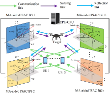
Figure 1: Illustration of the MA-enabled C-ISAC system.

Transmit signal. As shown in Fig.1, we consider a C-ISAC system that consists of $B$ dual-function radar and communication (DFRC) BSs. The set of BSs is denoted as $\mathcal{B}=\{1,\cdots,B\}$. Each BS is equipped with a uniform planar array (UPA) with $N=N_{x}\times N_{y}$ transmit MAs and $M=M_{x}\times M_{y}$ sensing receive MAs, where $N_{x}(M_{x})$ represents the number of horizontally transmit (receive sensing) MAs and the other $N_{y}(M_{y})$ represents the number of vertically transmit (receive sensing) MAs. The transmit set of MAs is represented as $\mathcal{N}=\{1,\cdots,N\}$, while the sensing receive set is defined as $\mathcal{M}=\{1,\cdots,M\}$. Each BS aims to transmit downlink signals to its associated users in the C-ISAC system. The BS collects echo signals reflected by point targets at its sensing receiver. Subsequently, all BSs forward this data to a central data processing center, where it undergoes joint target location estimation through data-level fusion. Common data-level approaches include maximum likelihood estimation (MLE) based fusion and weighted fusion techniques[22]. The integration of sensing information is crucial for multi-BS cooperative sensing[22]. Integrating sensing information is crucial for multi-BS cooperative sensing. In the C-ISAC system, the coordinates of the $b$-th BS are represented as $\boldsymbol{p}=[x_{b},y_{b},z_{b}]^{T}$. The C-ISAC system consists of $U$ single-antenna users and one sensing point target, where the set of users is denoted as $\mathcal{U}=\{1,\cdots,U\}$. We assume that the transmit signal of the $b$-th BS transmitter at time $n$ is given by

$$\boldsymbol{s}_{b}(n)=\boldsymbol{W}_{b}\boldsymbol{x}(n),b\in\mathcal{B},$$ (1)

where $\boldsymbol{W}_{b}=[\boldsymbol{w}_{b,1},\cdots,\boldsymbol{w}_{b,U}]\in\mathbb{C}^{N\times U}$ and $\boldsymbol{x}(n)=[x_{1}(n),\cdots,x_{U}(n)]^{T}\in\mathbb{C}^{U\times 1}$ denotes the communication signal from the $b$-th BS, which follows an independent normal distribution with mean $0$ and variance $1$. $\boldsymbol{W}_{b}$ represents the BS’s beamforming. $n\in(0,S]$ and $S$ denotes the duration of the interval.

MA channel. Let $\boldsymbol{h}_{b,u}(\tilde{\boldsymbol{t}}_{b})\in\mathbb{C}^{N\times 1}$ and $\boldsymbol{H}_{b^{\prime},b}(\tilde{\boldsymbol{r}}_{b^{\prime}},\tilde{\boldsymbol{t}}_{b})\in\mathbb{C}^{N\times M}$ represent the downlink communication channel and the sensing channel, respectively, where $\tilde{\boldsymbol{t}}_{b}=[\boldsymbol{t}_{b}^{1},\cdots,\boldsymbol{t}_{b}^{N}]\in\mathbb{R}^{3\times N}$, $\boldsymbol{t}_{b}^{n}=[x_{t,b}^{n},y_{t,b}^{n}]^{T}\in\mathcal{C}_{t,b}$ and $\tilde{\boldsymbol{r}}_{b}=[\boldsymbol{r}_{b}^{1},\cdots,\boldsymbol{r}_{b}^{M}]\in\mathbb{R}^{3\times N}$, $\boldsymbol{r}_{b}^{m}=[x_{r,b}^{m},y_{r,b}^{m}]\in\mathcal{C}_{r,b}$ denote the 3D coordinates of the positions of the communication transmit MA and the sensing receive MA of the $b$-th BS. $\mathcal{C}_{t,b}=[x_{t,b}^{\min},x_{t,b}^{\max}]\times[y_{t,b}^{\min},y_{t,b}^{\max}]$ and $\mathcal{C}_{r,b}=[x_{r,b}^{\min},x_{r,b}^{\max}]\times[y_{r,b}^{\min},y_{r,b}^{\max}]$. Both $\boldsymbol{h}_{b,u}(\tilde{\boldsymbol{t}}_{b})$ and $\boldsymbol{H}_{b^{\prime},b}(\tilde{\boldsymbol{r}}_{b^{\prime}},\tilde{\boldsymbol{t}}_{b})$ are assumed to be quasi-static block fading channels, with multipath components concentrated within a given region at a specific fading block located at an arbitrary position[23]. $\boldsymbol{h}_{b,u}(\tilde{\boldsymbol{t}}_{b})$ and $\boldsymbol{H}_{b^{\prime},b}(\tilde{\boldsymbol{r}}_{b^{\prime}},\tilde{\boldsymbol{t}}_{b})$ are characterized by the elevation angle and azimuth angle of departure (AoD), angle of arrival (AoAs) and MA position. Based on the field response channel model [24], $\boldsymbol{h}_{b,u}(\tilde{\boldsymbol{t}}_{b})$ and $\boldsymbol{H}_{b^{\prime},b}(\tilde{\boldsymbol{r}}_{b^{\prime}},\tilde{\boldsymbol{t}}_{b})$ are expressed as

$$\boldsymbol{h}_{b,u}(\tilde{\boldsymbol{t}}_{b})=\tilde{\boldsymbol{h}}_{b,u}^{H}\boldsymbol{A}_{b,u}(\tilde{\boldsymbol{t}}_{b}),$$

$$\boldsymbol{H}_{b^{\prime},b}(\tilde{\boldsymbol{r}}_{b^{\prime}},\tilde{\boldsymbol{t}}_{b})=\alpha_{b}\boldsymbol{a}(\tilde{\boldsymbol{r}}_{b^{\prime}})^{H}\boldsymbol{a}(\tilde{\boldsymbol{t}}_{b}),b,b^{\prime}\in\mathcal{B}.$$ (2)

Since the users are single-antenna, the field response matrix (FRM) only exists at the transmitting end of the communication channel. $\tilde{\boldsymbol{h}}_{b,u}\in\mathbb{C}^{L_{b,u}\times 1}$ is the complex channel gain, and $L_{b,u}$ represents the number of communication paths from the downlink the $b$-th BS to the $u$-th user. $\boldsymbol{A}_{b,u}(\tilde{\boldsymbol{t}}_{b})$ is the transmit FRM of the downlink channel. For the signal propagation distance difference of the $l_{b,u}$-th transmit path ($1\leq l_{b,u}\leq L_{b,u}$) between position $\tilde{\boldsymbol{t}}_{b}$ and the origin of the transmit region (i.e., $O_{b}$ in Fig.1), it can be expressed as $\rho_{l_{b,u}}^{b}(\boldsymbol{t}_{b}^{n})=x_{t,b}^{n}\cos\theta_{l_{b,u}}^{b}\cos\phi_{l_{b,u}}^{b}+y_{t,b}^{n}\cos\theta_{l_{b,u}}^{b}\sin\phi_{l_{b,u}}^{b}$, where the elevation and azimuth AoDs as $\theta_{l_{b,u}}^{b,u},\phi_{l_{b,u}}^{b,u}\in[0,\pi]$ respectively. Similarly, for the sensing signal between the target and the origin of the transmit region (i.e., $O_{b}$ in Fig.1), it can be expressed as $\rho^{b^{\prime}}(\boldsymbol{r}_{b^{\prime}}^{m})=x_{r,b}^{m}\cos\bar{\theta}^{b}\cos\bar{\phi}^{b}+y_{r,b}^{m}\cos\bar{\theta}^{b}\sin\bar{\phi}^{b}$, where the elevation and azimuth AoAs are denoted as $\bar{\theta}^{b},\bar{\phi}^{b}\in[0,\pi]$ respectively. According to the BS coordinates and target coordinates, $\rho^{b}(\boldsymbol{t}_{b}^{n})$ and $\rho^{b^{\prime}}(\boldsymbol{r}_{b^{\prime}}^{m})$ can be rewritten as (9) at the top of next page. Let $\lambda$ denote the carrier wavelength, and the phase difference of transmit MA and sensing receive MA can be calculated as $2\pi/\lambda\rho_{l_{b,u}}^{b}(\tilde{\boldsymbol{t}}_{b})$ and $2\pi/\lambda\rho^{b}(\tilde{\boldsymbol{r}}_{b})$, respectively. Therefore, the transmit and receive FRV characterizing the phase difference of $L_{b,u}$ transmit paths and sensing receive paths are expressed as

$$\boldsymbol{a}_{b,u}(\boldsymbol{t}_{b}^{n})=\left[e^{j2\pi/\lambda\rho_{1}^{b}(\boldsymbol{t}_{b}^{n})},\cdots,e^{j2\pi/\lambda\rho_{L_{b,u}}^{b}(\boldsymbol{t}_{b}^{n})}\right]^{T}\in\mathbb{C}^{L_{b,u}\times 1},$$

$$a(\boldsymbol{r}_{b}^{m})=e^{j2\pi/\lambda\rho^{b^{\prime}}(\boldsymbol{r}_{b^{\prime}}^{m})}\in\mathbb{C}^{1\times 1}.$$ (3)

Then, $\boldsymbol{A}_{b,u}(\tilde{\boldsymbol{t}}_{b})$ and $\boldsymbol{a}(\tilde{\boldsymbol{r}}_{b})$ are computed as

$$\boldsymbol{A}_{b,u}(\tilde{\boldsymbol{t}}_{b})=[\boldsymbol{a}_{b,u}(\boldsymbol{t}_{b}^{1}),\cdots,\boldsymbol{a}_{b,u}(\boldsymbol{t}_{b}^{N})]\in\mathbb{C}^{L_{b,u}\times N}$$

$$\boldsymbol{a}(\tilde{\boldsymbol{r}}_{b})=\left[e^{j2\pi/\lambda\rho_{1}^{b}(\boldsymbol{r}_{b}^{1})},\cdots,e^{j2\pi/\lambda\rho^{b^{\prime}}(\boldsymbol{r}_{b^{\prime}}^{m})}\right]^{T}\in\mathbb{C}^{M\times 1}.$$ (4)

Similarly, the transmit FRV for the sensing channel is expressed as

$$\boldsymbol{a}(\tilde{\boldsymbol{t}}_{b})=\left[e^{j2\pi/\lambda\rho_{1}^{b}(\boldsymbol{t}_{b}^{1})},\cdots,e^{j2\pi/\lambda\rho^{b}(\boldsymbol{t}_{b}^{N})}\right]^{T}\in\mathbb{C}^{M\times 1}.$$ (5)

Moreover, $\alpha_{b}$ denotes the reflection coefficient incorporating the effects of the radar cross section (RCS) from the transmit MAs at the $b$-th BS to the target to the sensing receive MAs at the $b^{\prime}$-th BS. This study investigates multi-static sensing in a C-ISAC system, where the BS ISAC transmitter and receiver are co-located. The receiver collects target reflection signals, and sends the results to the cloud server for collaborative sensing through data fusion. We focus on the stage where the BS has prior knowledge of the target parameters, obtained during detection. Using these parameters, the BS ISAC transmitter optimizes beamforming for target estimation and other sensing tasks. The cloud server also helps the BS determine its location, while the receiver reduces unwanted signals from the LoS path and clutter from static objects, assuming known NLoS paths. An LoS channel model in (2) is used to describe the BS-target link.

III-A Cooperative Communication Model

In the $n$-th time slot, the receive signal for the $u$-th user is represented as

$$y_{u}(n)=\sum\nolimits_{b=1}^{B}c_{b,u}\boldsymbol{h}_{b,u}(\tilde{\boldsymbol{t}}_{b})\boldsymbol{s}_{b}(n)+z_{u}(n),~c_{b,u}\in\{0,1\},$$ (6)

where $z_{u}(n)\sim\mathcal{CN}(0,\sigma_{u}^{2})$ represents the additive white Gaussian noise (AWGN) experienced by user $u$. Equation (6) shows that each user is influenced by interference from neighbouring BSs, highlighting the need for coordinated transmission beamforming to reduce this interference. In this context, $c_{b,u}$ serves as the selection variable. This communication link is not established if $c_{b,u}=0$ indicates the downlink from the $b$-th BS to the $u$-th user. In contrast, this communication link is established if $c_{b,u}=1$ represents the downlink from the $b$-th BS to the $u$-th user.

III-B Cooperative Sensing Model

The BS sensing receiver analyzes the receive target reflection signals and transmits the estimated results to the central processing unit (CPU). Utilizing previous target parameters and beamforming design enhances target estimation while considering the LoS channel model without considering clutter and non-target signals[25]. Thus, the receive sensing signal at the $b$-th BS during the $n$-th time slot is denoted as

$$\boldsymbol{y}_{b}(n)=\sum\nolimits_{b^{\prime}=1}^{B}\tilde{c}_{b}\boldsymbol{H}_{b^{\prime},b}(\tilde{\boldsymbol{r}}_{b^{\prime}},\tilde{\boldsymbol{t}}_{b})\boldsymbol{s}_{b}(n-\tau_{b,b^{\prime}})+\boldsymbol{z}_{b}(n),$$

$$~\tau_{b,b^{\prime}}=\left\{\begin{matrix}0,&b=b^{\prime}\\ \tau_{b,b^{\prime}},&b\neq b^{\prime}\end{matrix}\right.~b,b^{\prime}\in\mathcal{B},$$ (7)

where $t_{b^{\prime},b}$ denotes the propagation delay measurement from the $b$-th BS ISAC transmitter to the target and from the target to the $b^{\prime}$-th BS sensing receiver[25], and $\tau_{b,b^{\prime}}$ is given by

$$\tau_{b,b^{\prime}}=\hat{t}_{b,b^{\prime}}+\xi_{b,b^{\prime}}+\bar{\xi}_{b,b^{\prime}},\xi_{b,b^{\prime}}=\Delta\xi_{b}-\Delta\xi_{b^{\prime}},$$ (8)

where $\Delta\xi_{b}$ and $\Delta\xi_{b^{\prime}}$ denote the TS error between the $b$/$b^{\prime}$-th BS and the reference clock. According to [25], the TS error $\xi_{b,b^{\prime}}$ is a random variable, and it can be modeled as following a Gaussian distribution with mean $0$ and variance $\sigma^{2}_{\xi}$. $\hat{t}_{b,b^{\prime}}$ represents the transmission delay from the $b$-th BS, passing through the target and reflecting the $b^{\prime}$-th BS. $\bar{\xi}_{b,b^{\prime}}$ is the measurement noise. Finally, all mathematical symbols are defined in TABLE I.

$$\rho^{b}(\boldsymbol{t}_{b}^{n})=x_{n}^{b}\sin\underbrace{\left(\arctan\left((x_{T}-x_{b})/(x_{T}-y_{b})\right)+\pi\right)}_{\theta_{b}}\cos\underbrace{\left(\arctan\left(z_{b}/\sqrt{(x_{T}-x_{b})^{2}+(x_{T}-y_{b})^{2}}\right)+\pi\right)}_{\phi_{b}}+y_{n}^{b}\cos(\arctan((x_{T}-x_{b})/$$

$$(x_{T}-y_{b}))+\pi)\sin\left(\arctan\left(z_{b}/\sqrt{(x_{T}-x_{b})^{2}+(x_{T}-y_{b})^{2}}\right)+\pi\right),$$

$$\rho^{b^{\prime}}(\boldsymbol{r}_{b^{\prime}}^{m})=x_{m}^{b^{\prime}}\sin\underbrace{\left(\arctan\left((x_{T}-x_{b^{\prime}})/(x_{T}-y_{b^{\prime}})\right)+\pi\right)}_{\bar{\theta}_{b^{\prime}}}\cos\underbrace{\left(\arctan\left(z_{b^{\prime}}/\sqrt{(x_{T}-x_{b^{\prime}})^{2}+(x_{T}-y_{b^{\prime}})^{2}}\right)+\pi\right)}_{\bar{\phi}_{b}}+y_{m}^{b^{\prime}}\cos(\arctan((x_{T}-x_{b^{\prime}})/$$

$$(x_{T}-y_{b^{\prime}}))+\pi)\sin\left(\arctan\left(z_{b^{\prime}}/\sqrt{(x_{T}-x_{b^{\prime}})^{2}+(x_{T}-y_{b^{\prime}})^{2}}\right)+\pi\right).$$ (9)

Symbol	Description
$\mathcal{B}/\mathcal{U}$	Set of all BSs/users
$B/U$	Number of BSs/users
$\mathcal{N}/\mathcal{M}$	Set of all transmit MAs/receive MAs
$N/M$	Number of transmit MAs/receive MAs
$\boldsymbol{W}_{b}$	Beamforming of the $b$-th BS
$S$	Symbol duration
$\tilde{\boldsymbol{t}}_{b}/\tilde{\boldsymbol{r}}_{b}$	Position of transmit MAs/receive MAs
$\mathcal{C}_{t,b}/\mathcal{C}_{r,b}$	Movable region of transmit MAs/receive
	MAs
$\boldsymbol{h}_{b,u}(\tilde{\boldsymbol{t}}_{b})$	Channel BS-to-user
$\boldsymbol{H}_{b^{\prime},b}(\tilde{\boldsymbol{r}}_{b^{\prime}},\tilde{\boldsymbol{t}}_{b})$	Channel BS-to-BS
$L_{b,u}$	Number of channel paths
$\theta_{l_{b,u}}^{b,u}$/$\phi_{l_{b,u}}^{b,u}$	Elevation and azimuth AoDs of
	communication signal
$\bar{\theta}^{b}$/$\bar{\phi}^{b}$	Elevation and azimuth AoDs of sensing signal
$\theta^{b}$/$\phi^{b}$	Elevation and azimuth AoAs of sensing signal
$c_{b,u}/\tilde{c}_{b}$	Selection factor
$t_{b^{\prime},b}$	Propagation delay measurement
$\Delta\xi_{b}$/$\Delta\xi_{b^{\prime}}$	TS error

TABLE I: Summary of Notations.

IV C-ISAC with Imperfect CSI and TS error

The practical deployment of the C-ISAC system depends heavily on the availability of CSI and TS between different BSs. However, due to imperfect CSI and TS data at these BSs, both are prone to errors. This section analyzes the worst-case communication rate constraints related to CSI estimation errors and the HCRLB concerning TS errors and their impact on sensing accuracy under imperfect conditions.

IV-A Worst-case Achievable Rate with Imperfect CSI

According to [26], introducing a communication rate constraint is essential to ensure the system meets required throughput and reliability. This constraint ensures the system operates within available bandwidth and power while maintaining acceptable quality of service (QoS) for users [27]. We aim to balance power consumption and system robustness, particularly in the presence of interference and noise. This balance is the key to optimizing resource allocation and achieving desired performance in practical systems [14]. In summary, this paper introduces a communication rate constraint, which is expressed as based on the receive signal in (6)

$$R_{u}=\log_{2}\left(1+\sum\nolimits_{b=1}^{B}|c_{b,u}\boldsymbol{h}_{b,u}(\tilde{\boldsymbol{t}}_{b})\boldsymbol{w}_{b,u}|^{2}/\left(\sum\nolimits_{b=1}^{B}\sum\nolimits_{u^{\prime}=1,u^{\prime}\neq u}^{U}\right.\right.$$

$$\left.\left.|c_{b,u^{\prime}}\boldsymbol{h}_{b,u^{\prime}}(\tilde{\boldsymbol{t}}_{b})\boldsymbol{w}_{b,u^{\prime}}|^{2}\right)+\sigma_{b}^{2}\right)\geq\gamma_{u}.$$ (10)

Based on[28], the relationship between the actual CSI, the estimated CSI error, and the true CSI is expressed as

$$\boldsymbol{h}_{b,u}(\tilde{\boldsymbol{t}}_{b})=\hat{\boldsymbol{h}}_{b,u}(\tilde{\boldsymbol{t}}_{b})+\Delta\boldsymbol{h}_{b,u},\|\Delta\boldsymbol{h}_{b,u}\|\leq\epsilon_{b,u}.$$ (11)

The existing MA-based channel estimation techniques reconstruct the channel by obtaining the AoA, AoD, and channel gain[29]. Therefore, we have

$$\theta_{l_{b,u}}^{b}=\hat{\theta}_{l_{b,u}}^{b}+\Delta\theta_{l_{b,u}}^{b},\phi_{l_{b,u}}^{b}=\hat{\phi}_{l_{b,u}}^{b}+\Delta\phi_{l_{b,u}}^{b},\tilde{\boldsymbol{h}}_{b,u}=\hat{\tilde{\boldsymbol{h}}}_{b,u}+\Delta\tilde{\boldsymbol{h}}_{b,u},$$

$$|\Delta\theta_{l_{b,u}}^{b}|<\epsilon_{\theta},|\Delta\phi_{l_{b,u}}^{b}|<\epsilon_{\phi},\|\Delta\tilde{\boldsymbol{h}}_{b,u}\|\leq\bar{\epsilon}_{b,u}.$$ (12)

Although $\epsilon_{\theta}$, $\epsilon_{\phi}$ and $\bar{\epsilon}_{b,u}$ are known, due to the nonlinear relationship between the estimation errors $\epsilon_{\theta}$, $\epsilon_{\phi}$ and $\bar{\epsilon}_{b,u}$ and true channel $\boldsymbol{h}_{b,u}(\tilde{\boldsymbol{t}}_{b})$, the range of the channel estimation error $\epsilon_{b,u}$ remains uncertain. According to (11), communication rate constraint (11) is rewritten as

$$R_{u}=\log_{2}\left(1+\sum\nolimits_{b=1}^{B}|c_{b,u}(\hat{\boldsymbol{h}}_{b,u}(\tilde{\boldsymbol{t}}_{b})+\Delta\boldsymbol{h}_{b,u})^{H}\boldsymbol{w}_{b,u}|^{2}/\left(\sum\nolimits_{b=1}^{B}\right.\right.$$

$$\left.\left.\sum\nolimits_{u^{\prime}=1,u^{\prime}\neq u}^{U}|c_{b,u^{\prime}}(\hat{\boldsymbol{h}}_{b,u^{\prime}}(\tilde{\boldsymbol{t}}_{b})+\Delta\boldsymbol{h}_{b,u^{\prime}})^{H}\boldsymbol{w}_{b,u^{\prime}}|^{2}\right)+\sigma_{b}^{2}\right)\geq\gamma_{u}.$$ (13)

From the communication rate constraint in [28], we note that $\Delta\boldsymbol{h}_{b,u^{\prime}}$ appears in both the interference and signal gain terms. According to the worst-case robust optimization theory derived in[28], if the feasible region of the worst-case communication rate constraint is smaller than that of the actual communication rate constraint, then the worst-case communication rate constraint encountered during the optimization process will be more restrictive than the actual worst-case constraint. This situation leads to a more robust and feasible region for the communication rate constraint. A smaller feasible set means which reduces the sensitivity of the problem to variations or uncertainties in the input data. With fewer options, the influence of data fluctuations on the optimal solution is minimized, resulting in more consistent performance[28]. Consequently, we present the following theorem.

Theorem 1.

The communication rate constraint in (13) can be scaled as a worst-case communication rate constraint, and it is expressed as

$$\underbrace{A(\boldsymbol{w}_{b,u})/B(\boldsymbol{w}_{b,u^{\prime}})}_{C(\boldsymbol{w}_{b,u},\boldsymbol{w}_{b,u^{\prime}})}\geq(2^{\gamma_{u}}-1),$$ (14)

where $A(\boldsymbol{w}_{b,u})$ and $B(\boldsymbol{w}_{b,u^{\prime}})$ are given by

$$A(\boldsymbol{w}_{b,u})=$$

$$\sum\nolimits_{b=1}^{B}(c_{b,u}|\hat{\boldsymbol{h}}_{b,u}^{H}(\tilde{\boldsymbol{t}}_{b})\boldsymbol{w}_{b,u}|)^{2}-(c_{b,u}(N\|\hat{\tilde{\boldsymbol{h}}}_{b,u}\|^{2}+2NL_{b,u}\bar{\epsilon}_{b,u}))$$

$$|\boldsymbol{w}_{b,u}|^{2})-2c_{b,u}^{2}|\hat{\boldsymbol{h}}_{b,u}^{H}(\tilde{\boldsymbol{t}}_{b})\boldsymbol{w}_{b,u}|\sqrt{(N\|\hat{\tilde{\boldsymbol{h}}}_{b,u}\|^{2}+2NL_{b,u}\bar{\epsilon}_{b,u})\|\boldsymbol{w}_{b,u}\|^{2}}$$

$$B(\boldsymbol{w}_{b,u^{\prime}})=\left(\sum\nolimits_{b=1}^{B}\right.\sum\nolimits_{u^{\prime}=1,u^{\prime}\neq u}^{U}(c_{b,u^{\prime}}|\hat{\boldsymbol{h}}_{b,u^{\prime}}^{H}(\tilde{\boldsymbol{t}}_{b})\boldsymbol{w}_{b,u^{\prime}}|)^{2}+c_{b,u}^{2}$$

$$(N\|\hat{\tilde{\boldsymbol{h}}}_{b,u^{\prime}}\|^{2}+2NL_{b,u^{\prime}}\bar{\epsilon}_{b,u^{\prime}})\left.\left.\times\|\boldsymbol{w}_{b,u^{\prime}}\|^{2}+2c_{b,u^{\prime}}^{2}|\hat{\boldsymbol{h}}_{b,u^{\prime}}^{H}(\tilde{\boldsymbol{t}}_{b})\boldsymbol{w}_{b,u^{\prime}}|\right.\right.$$

$$\left.\left.\sqrt{(N\|\hat{\tilde{\boldsymbol{h}}}_{b,u^{\prime}}\|^{2}+2NL_{b,u^{\prime}}\bar{\epsilon}_{b,u^{\prime}})\|\boldsymbol{w}_{b,u^{\prime}}\|^{2}}\right)+\sigma_{b}^{2}\right).$$ (15)

This proof is given in Appendix A.

IV-B Sensing Accuracy with TS Errors

In the following, we focus on the target position $\boldsymbol{p}=[p_{x},p_{y}]^{T}$ as the interested parameters. The Cramér-Rao Lower Bound (CRLB) is used to quantify estimation performance as the lower bound on the variance of any unbiased estimator. Based on Section III, TS errors are inevitable and significantly affect target estimation. Therefore, we derive the CRLB with TS errors to establish tight performance bounds. Specifically, each BS sensing receiver samples the receive signal $\bar{S}$ over $S$, yielding samples ${\boldsymbol{y}_{b}(n_{1}),\cdots,\boldsymbol{y}_{b}(n_{\bar{S}})}$. Let $\mathcal{S}=\{n_{1},\cdots,n_{\bar{S}}\}$ denote the sampling times. The frequency domain signal $\boldsymbol{y}_{b}(n_{s})$ is obtained via discrete Fourier transform (DFT)[8], the frequency-domain signal of $\boldsymbol{y}_{b}(n_{s})$, $\forall t_{s}\in\mathcal{S}$ is obtained as

$$\bar{\boldsymbol{y}}_{b}(f_{s})=\sum\nolimits_{b^{\prime}=1}^{B}\bar{c}_{b}\boldsymbol{H}_{b,b^{\prime}}(\tilde{\boldsymbol{r}}_{b^{\prime}},\tilde{\boldsymbol{t}}_{b})\boldsymbol{W}_{b}e^{-jf_{s}\tau_{b,b^{\prime}}}\boldsymbol{s}_{b}(f_{s})+\bar{\boldsymbol{z}}_{b}(f_{s}).$$ (16)

Then, the signal receive by the $b$-th ISAC BS sensing receiver is expressed in the frequency domain as

$$\underbrace{\left[\begin{matrix}\bar{\boldsymbol{y}}_{b}(f_{1})\\ \vdots\\ \bar{\boldsymbol{y}}_{b}(f_{\bar{S}})\end{matrix}\right]}_{\tilde{\boldsymbol{y}}_{b}}=\underbrace{\left[\begin{matrix}\sum\nolimits_{b^{\prime}=1}^{B}\bar{c}_{b}\boldsymbol{H}_{b,b^{\prime}}(\tilde{\boldsymbol{r}}_{b^{\prime}},\tilde{\boldsymbol{t}}_{b})\boldsymbol{W}_{b}e^{-jf_{1}\tau_{b,b^{\prime}}}\boldsymbol{s}_{b}(f_{1})\\ \vdots\\ \sum\nolimits_{b^{\prime}=1}^{B}\bar{c}_{b}\boldsymbol{H}_{b,b^{\prime}}(\tilde{\boldsymbol{r}}_{b^{\prime}},\tilde{\boldsymbol{t}}_{b})\boldsymbol{W}_{b}e^{-jf_{\bar{S}}\tau_{b,b^{\prime}}}\boldsymbol{s}_{b}(f_{\bar{S}})\\ \end{matrix}\right]}_{\tilde{\boldsymbol{x}}_{b}}+\tilde{\boldsymbol{z}}_{b},$$ (17)

where $\tilde{\boldsymbol{z}}_{b}=[\bar{\boldsymbol{z}}_{b}(f_{1}),\cdots,\bar{\boldsymbol{z}}_{b}(f_{\bar{S}})]^{T}$, $\tilde{\boldsymbol{z}}_{b}\sim\mathcal{CN}(0,\sigma_{b}^{2}\boldsymbol{I})$. According to the frequency-domain sensing signal expression in (17), both the position parameter $\boldsymbol{p}_{T}$ and synchronization parameter $\boldsymbol{\xi}_{b}=[\xi_{1,b},\cdots,\xi_{B,b}]^{T}\sim\mathcal{N}(\boldsymbol{0},\sigma_{\xi}^{2}\boldsymbol{I})$ are unknown. In this case, the sensing receiver signal at the $b$-th BS is used to jointly estimate a total of $B+2$ parameters. As is well known, the HCRLB is more suitable for determining the lower bound of the estimation accuracy for multi-source parameters[30, 31]. Since the HCRLB provides a lower bound on the mean squared error (MSE) for any unbiased estimator of deterministic parameters and any estimator of stochastic parameters, deriving the HCRLB for parameters $\boldsymbol{p}_{T}$ and $\boldsymbol{\xi}_{b}$ requires first determining the MSE based on the sensing receive signal. Therefore, the MSE lower bound for the position parameter $\boldsymbol{p}_{T}$ and synchronization parameter $\boldsymbol{\xi}_{b}$, based on the sensing receive signal $\tilde{\boldsymbol{y}}_{b}$, is expressed as follows:

$$\mathrm{Cov}_{\tilde{\boldsymbol{y}}_{b}}((\hat{\boldsymbol{\zeta}}_{b}-\boldsymbol{\zeta}_{b})(\hat{\boldsymbol{\zeta}}_{b}-\boldsymbol{\zeta}_{b})^{T})\succeq\underbrace{\mathbb{E}\left\{\left(\frac{\partial\log p(\tilde{\boldsymbol{y}}_{b};\boldsymbol{\zeta}_{b})}{\partial\boldsymbol{\zeta}_{b}}\right)\right.}_{\text{hybrid Fisher information matrix}}$$

$$\underbrace{\left.\left(\frac{\partial\log p(\tilde{\boldsymbol{y}}_{b};\boldsymbol{\zeta}_{b})}{\partial\boldsymbol{\zeta}_{b}}\right)^{T}\right\}}_{\text{hybrid FIM}}.$$ (18)

The HFIM can be divided into the observed FIM (OFIM) and the prior FIM (PFIM), and the expression is given as follows:

$$\mathbb{E}\left\{\left(\frac{\partial\log p(\tilde{\boldsymbol{y}}_{b};\boldsymbol{\zeta}_{b})}{\partial\boldsymbol{\zeta}_{b}}\right)\left(\frac{\partial\log p(\tilde{\boldsymbol{y}}_{b};\boldsymbol{\zeta}_{b})}{\partial\boldsymbol{\zeta}_{b}}\right)^{T}\right\}=$$

$$\underbrace{-\mathbb{E}_{\tilde{\boldsymbol{y}}_{b}|\boldsymbol{\zeta}_{b}}\left\{\left(\frac{\partial^{2}\log p(\tilde{\boldsymbol{y}}_{b}|\boldsymbol{\zeta}_{b})}{\partial\boldsymbol{\zeta}_{b}\partial\boldsymbol{\zeta}_{b}^{T}}\right)\right\}}_{\text{OFIM}~\boldsymbol{\Xi}_{O}}\underbrace{-\mathbb{E}_{\boldsymbol{\zeta}_{b}}\left\{\left(\frac{\partial^{2}\log p(\Delta\boldsymbol{\xi}_{b})}{\partial\boldsymbol{\zeta}_{b}\partial\boldsymbol{\zeta}_{b}^{T}}\right)\right\}}_{\text{PFIM}~\boldsymbol{\Xi}_{P}},$$ (19)

in which $p(\tilde{\boldsymbol{y}}_{b};\boldsymbol{\zeta}_{b})$ and $p(\Delta\boldsymbol{\xi}_{b})$ are expressed as

$$p(\tilde{\boldsymbol{y}}_{b};\boldsymbol{\zeta}_{b})=\left(1/\left(2\pi\sigma_{b}^{2L_{r}\bar{S}}\right)^{L_{r}/2}\right)e^{-\frac{1}{2\sigma_{b}^{2}}(\tilde{\boldsymbol{y}}_{b}-\tilde{\boldsymbol{x}}_{b})^{T}(\tilde{\boldsymbol{y}}_{b}-\tilde{\boldsymbol{x}}_{b})}$$ (20)

and

$$p(\Delta\boldsymbol{\xi}_{b})=\left(1/(2\pi\sigma_{\xi}^{2M})^{M/2}\right)e^{-\sigma_{\xi}^{2}/2\Delta\boldsymbol{\xi}_{b}^{T}\Delta\boldsymbol{\xi}_{b}}.$$ (21)

Then, the HCRLB matrix corresponding to the sensing receiver at the $b$-th BS can be expressed as

$$\boldsymbol{{\mathrm{HCRLB}}}_{b}(\boldsymbol{\zeta}_{b})=[\mathrm{HFIM}_{b}(\boldsymbol{\zeta}_{b})]^{-1}.$$ (22)

Based on the analysis, the OFIM and the PFIM represent the contributions of the observed data and prior knowledge to the estimation error bounds, respectively. Therefore, compared to the CRLB, the HCRLB incorporates additional prior Fisher information, which enables a more accurate determination of the lower bound of the estimation error, thereby providing a more precise performance evaluation. To simplify the derivation of the HCRLB for estimating the target position $\boldsymbol{\xi}_{b}$, we divide the hybrid FIM used for estimating $\boldsymbol{\zeta}_{b}$ into multiple sub-blocks

$$\mathrm{HFIM}_{b}(\boldsymbol{\zeta}_{b})=\left[\begin{matrix}\frac{\partial^{2}\log p(\tilde{\boldsymbol{y}}_{b};\boldsymbol{\zeta}_{b})}{\partial\boldsymbol{p}\partial\boldsymbol{p}}&\frac{\partial^{2}\log p(\tilde{\boldsymbol{y}}_{b};\boldsymbol{\zeta}_{b})}{\partial\boldsymbol{p}\partial\Delta\boldsymbol{\xi}_{b}}\\ \left(\frac{\partial^{2}\log p(\tilde{\boldsymbol{y}}_{b};\boldsymbol{\zeta}_{b})}{\partial\boldsymbol{p}\partial\Delta\boldsymbol{\xi}_{b}}\right)^{T}&\frac{\partial^{2}\log p(\tilde{\boldsymbol{y}}_{b};\boldsymbol{\zeta}_{b})}{\partial\Delta\boldsymbol{\xi}_{b}\partial\Delta\boldsymbol{\xi}_{b}}\end{matrix}\right],$$ (23)

where the elements of $\frac{\partial^{2}\log p(\tilde{\boldsymbol{y}}_{b};\boldsymbol{\zeta}_{b})}{\partial\boldsymbol{p}\partial\boldsymbol{p}}$, $\frac{\partial^{2}\log p(\tilde{\boldsymbol{y}}_{b};\boldsymbol{\zeta}_{b})}{\partial\boldsymbol{p}\partial\Delta\boldsymbol{\xi}_{b}}$ , and $\frac{\partial^{2}\log p(\tilde{\boldsymbol{y}}_{b};\boldsymbol{\zeta}_{b})}{\partial\Delta\boldsymbol{\xi}_{b}\partial\Delta\boldsymbol{\xi}_{b}}$ are derived in the Appendix B. It is worth noting that according to the derivations in the Appendix B, each element of $\mathrm{HFIM}_{b}(\boldsymbol{\zeta}_{b})$ is a quadratic function of $\boldsymbol{w}=[\boldsymbol{w}_{1}^{H},\cdots,\boldsymbol{w}_{B}^{H}]^{H}$. Then, the HCRLB matrix of target position $\boldsymbol{p}$ corresponding to the $b$-th BS sensing receiver is calculated as

$$\boldsymbol{{\mathrm{HCRLB}}}_{b}(\boldsymbol{p})=(\underbrace{\frac{\partial^{2}\log p(\tilde{\boldsymbol{y}}_{b};\boldsymbol{\zeta}_{b})}{\partial\boldsymbol{p}\partial\boldsymbol{p}}}_{\boldsymbol{\Xi}^{b}_{\boldsymbol{p}\boldsymbol{p}}}-\underbrace{\frac{\partial^{2}\log p(\tilde{\boldsymbol{y}}_{b};\boldsymbol{\zeta}_{b})}{\partial\boldsymbol{p}\partial\Delta\boldsymbol{\xi}_{b}}}_{\boldsymbol{\Xi}^{b}_{\boldsymbol{p}\Delta\boldsymbol{\xi}_{b}}}$$

$$(\underbrace{\frac{\partial^{2}\log p(\tilde{\boldsymbol{y}}_{b};\boldsymbol{\zeta}_{b})}{\partial\Delta\boldsymbol{\xi}_{b}\partial\Delta\boldsymbol{\xi}_{b}}}_{\boldsymbol{\Xi}^{b}_{\Delta\boldsymbol{\xi}_{b}\Delta\boldsymbol{\xi}_{b}}})^{-1}(\frac{\partial^{2}\log p(\tilde{\boldsymbol{y}}_{b};\boldsymbol{\zeta}_{b})}{\partial\boldsymbol{p}\partial\Delta\boldsymbol{\xi}_{b}})^{T})^{-1}.$$ (24)

To rigorously investigate an impact of TS errors on target position estimation, we apply the matrix inversion Theorem 2[30] to expand equation (19 ) into equation (21) at the top of the next page. It is well known that the CRLB is asymptotically tight under certain conditions, which is typically achieved through maximum likelihood estimation when the signal-to-noise ratio (SNR) and/or observation time are sufficiently large. However, the HCRLB is not always asymptotically tight, even though it may approach the optimal lower bound under certain conditions. Before using the HCRLB to assess estimation performance, its asymptotic tightness must be verified, ensuring the existence of an unbiased estimator whose MSE equals the HCRLB[8]. Consequently, according to [32], the HCRLB is given in (25) at the top of the next page and the asymptotically tight is proved in [30].

$$\boldsymbol{{\mathrm{HCRLB}}}_{b}(\boldsymbol{p})=\underbrace{(\boldsymbol{\Xi}_{\boldsymbol{p}\boldsymbol{p}}^{b})^{-1}}_{\text{CRLB with target position}}+\underbrace{(\boldsymbol{\Xi}_{\boldsymbol{p}\boldsymbol{p}}^{b})^{-1}\boldsymbol{\Xi}_{\boldsymbol{p}\Delta\boldsymbol{\xi}_{b}}^{b}(\boldsymbol{\Xi}_{\Delta\boldsymbol{\xi}_{b}\Delta\boldsymbol{u}_{b}}^{b}-(\boldsymbol{\Xi}_{\boldsymbol{p}\Delta\boldsymbol{\xi}_{b}}^{b})^{T}(\boldsymbol{\Xi}_{\boldsymbol{p}\boldsymbol{p}}^{b})^{-1}\boldsymbol{F}_{\boldsymbol{p}\Delta\boldsymbol{\xi}_{b}}^{b})^{-1}(\boldsymbol{\Xi}_{\boldsymbol{p}\Delta\boldsymbol{u}_{b}}^{b})^{T}(\boldsymbol{\Xi}_{\boldsymbol{p}\boldsymbol{p}})^{-1}}_{\text{Extra component due to TS errors}}.$$ (25)

The HCRLB matrix represents the minimum variance of an unbiased estimator for a parameter, with its trace providing a lower bound on overall estimation performance. In a communication and sensing integration system, the goal is to minimize power through coordinated beamforming at the BS while accounting for TS errors. The HCRLB matrix is used to evaluate target estimation performance and as a constraint to balance sensing and communication within the power budget. The optimization problem is framed as a robust power minimization problem, where the HCRLB constraint limits sensing error and the power allocation meets the worst-case communication rate constraint. Thus, the problem is given by

$$\min_{\boldsymbol{W}_{b},\tilde{\boldsymbol{t}}_{b},\tilde{\boldsymbol{r}}_{b},c_{b},c_{b,u}} ~\sum\nolimits_{b=1}^{B}\|\boldsymbol{W}_{b}\|^{2},$$ (26a)

s.t. $$\mathrm{tr}\{\boldsymbol{{\mathrm{HCRLB}}}_{b}(\boldsymbol{p})\}\leq\gamma_{b},~\forall~b\in\mathcal{B}$$ (26b)

$$C(\boldsymbol{w}_{b,u},\boldsymbol{w}_{b,u^{\prime}})\geq(2^{\gamma_{u}}-1),$$ (26c)

$$c_{b,u}=c_{b}\in\{0,1\},\forall~b\in\mathcal{B},u\in\mathcal{U},$$ (26d)

$$\tilde{\boldsymbol{t}}_{b}\in\mathcal{C}_{t,b},\tilde{\boldsymbol{r}}_{b}\in\mathcal{C}_{r,b}$$ (26e)

$$\|\boldsymbol{t}_{b}^{n_{1}}-\boldsymbol{t}_{b}^{n_{2}}\|_{2}\geq D,$$ (26f)

$$\|\boldsymbol{r}_{b}^{m_{1}}-\boldsymbol{r}_{b}^{m_{2}}\|_{2}\geq D,$$ (26g)

where $\gamma_{b}$ is the sensing accuracy constraint of BS sensing receiver $b$. It is observed that problem (26b) is non-convex, which is difficult to tackle due to the transmit power minimization problem. Moreover, communication constraint (26c) is non-convex. (26d) is the BS selection constraint. (26e) is the movable region constraint of the MAs. (26f) and (26g) are the minimum spacing constraints for MAs.

V Proposed CDRL Algorithm

This paper models the optimization problem of the C-ISAC system as a constrained Markov decision process (CMDP), considering both communication and sensing channels. In a time slot $n$, each BS selects an action based on the observed state. After the action, the BS receives feedback in the form of a reward and a cost, and the environment transits to the next state with a certain probability. This process repeats as the BS observes a new state and makes decisions based on it. The following sections will describe the key components of the proposed CMDP model.

V-A Proposed CMDP Model

State Space: The state observed by the BS can be represented as $\boldsymbol{s}^{(n)}=\{\hat{\boldsymbol{h}}_{b,u},\boldsymbol{H}_{b^{\prime},b}|b\in\mathcal{B},u\in\mathcal{U}\}$, which includes the acquired communication and sensing channels.

Action Space: Since the environment typically does not undergo drastic changes between consecutive time slots, we set action space as $\boldsymbol{a}^{(n)}=\{\mathrm{Re}(\boldsymbol{W}_{b}),\mathrm{Im}(\boldsymbol{W}_{b}),\tilde{\boldsymbol{t}}_{b},\tilde{\boldsymbol{r}}_{b},c_{b},c_{b,u}|b\in\mathcal{B},u\in\mathcal{U}\}$.

Reward and cost functions: In order to enable all BSs to minimize transmit power while satisfying the sensing and communication rate constraints, we design the instantaneous reward and cost functions as follows:

$$r^{(n)}=-\sum\nolimits_{b=1}^{B}\|\boldsymbol{W}_{b}^{(n)}\|^{2}-\delta_{1}\sum_{b=1}^{B}\sum_{u=1}^{U}\prod_{b,u}(\text{if}~c_{b,u}=c_{b},\prod_{b,u}=1~$$

$$\text{else}\prod_{b,u}=0)-\delta_{2}\sum_{b=1}^{B}\prod_{t,b}(\text{if}~\tilde{\boldsymbol{t}}_{b}\in\mathcal{C}_{t,b},\prod_{b}=1~\text{else}~\prod_{b}=0)-$$

$$\delta_{3}\sum_{b=1}^{B}\prod_{r,b}(\text{if}~\tilde{\boldsymbol{r}}_{b}\in\mathcal{C}_{r,b}~\text{else}~\prod_{b}=0),$$

$$c^{(n)}=\mathrm{tr}\{\boldsymbol{{\mathrm{HCRLB}}}_{b}(\boldsymbol{p})\}^{(n)}-C(\boldsymbol{w}_{b,u},\boldsymbol{w}_{b,u^{\prime}})^{(n)}-\|\boldsymbol{t}_{b}^{n_{1}}-\boldsymbol{t}_{b}^{n_{2}}\|_{2}^{(n)}$$

$$-\|\boldsymbol{r}_{b}^{m_{1}}-\boldsymbol{r}_{b}^{m_{2}}\|_{2}^{(n)},$$ (27)

where $\delta_{1}$, $\delta_{2}$, and $\delta_{3}$ are weighting factors that control the influence of BS selection and movable region of MAs in the overall reward. Following the strategy parameterized by $\mu$, the long-term cumulative reward and cost starting from $n_{0}$ are

$$R(\mu)=\mathbb{E}_{\mu}\left[\sum\nolimits_{n=n_{0}}^{S}\gamma^{n-n_{0}}r^{(n)}\right],C(\mu)=\mathbb{E}_{\mu}\left[\sum\nolimits_{n=n_{0}}^{S}\gamma^{n-n_{0}}c^{(n)}\right],$$ (28)

where $\gamma$ denotes the discounting factor. The objective of the BS in this CMDP is

$$\mu^{*}=\arg\min_{\mu}R(\mu),C(\mu)\leq\Gamma_{c}=\sum\nolimits_{n=n_{0}}^{T}-\gamma^{n-n_{0}}\eta_{c},$$ (29)

where $\eta_{c}=(\gamma_{b}+2^{\gamma_{u}}-1+2D)$ is the threshold for SE in each subframe, corresponding to the constraint in (9a).

4) Reward and cost functions: In the $n$-th time slot, the state $\boldsymbol{s}^{(n+1)}=\{\boldsymbol{S}_{H}^{(n+1)}\}$ is evolved as $\boldsymbol{S}_{H}^{(n+1)}=\boldsymbol{S}_{H}^{(n)}$.

V-B Proposed Algorithm

As the number of users and BSs grows, the action space expands exponentially, making training harder[33]. Traditional algorithms like DQN struggle with high-dimensional spaces and cost constraints. To tackle this, we use an actor-critic framework with primal-dual updates and Wolpertinger-based action selection.

To address this constrained optimization problem, we design reward and cost evaluation networks parameterized by $\eta_{1}$ and $\eta_{2}$, which map from the joint state and action spaces to the corresponding rewards and costs, thus serving the purpose of action evaluation: $Q_{1}(\boldsymbol{s}^{(n)},\boldsymbol{a}^{(n)}|\eta_{1})$ and $Q_{2}(\boldsymbol{s}^{(t)},\boldsymbol{a}^{(n)}|\eta_{2})$. The actor network $\kappa$ is parameterized by $\eta_{3}$, which maps the state space to actions $\kappa(\boldsymbol{s}^{(n)}|\eta_{3})=\boldsymbol{a}^{(n)}$. To reduce fluctuations in the target values during training and accelerate convergence, we employ target networks $Q_{1}^{\prime}$, $Q_{2}^{\prime}$, and $\kappa^{\prime}$, parameterized by $\eta_{1}^{\prime}$, $\eta_{2}^{\prime}$, and $\eta_{3}^{\prime}$, respectively. To solve the CMDP presented in (30), we first apply the Lagrangian relaxation method to transform the problem in (29) into an unconstrained problem as follows:

$$\min_{\zeta\geq 0}\max_{\eta_{3}}[R(\eta_{3})-\zeta(C(\eta_{3})-\Gamma_{c})],$$ (30)

where the dual variable $\zeta$ acts as an additional parameter that is updated during the optimization process.

Action Selection: With $\kappa$ held constant, the BS aims to maximize the unconstrained objective in Eq.(30). Consequently, one action $\boldsymbol{a}^{*}$ is chosen from the set of $K$ possible actions and executed by the BS at time slot $n$, based on the current feedback from the critic networks.

$$\boldsymbol{a}^{*(t)}=\arg\max_{\boldsymbol{a}\in\hat{\mathcal{A}}}[Q_{1}(\boldsymbol{s}^{(n)},\boldsymbol{a}|\eta_{1})-\lambda(Q_{2}(\boldsymbol{s}^{(n)},\boldsymbol{a}|\eta_{2})-\Gamma_{c})].$$ (31)

The transition tuple $(\boldsymbol{s}^{(n)},\boldsymbol{a}^{(n)},r^{(n)},c^{(n)},\boldsymbol{s}^{(n+1)})$ is stored in a memory replay buffer $\mathcal{M}$ for network updating.

Primal-Dual Network Update: To facilitate the model training, we adopt a primal dual-deep deterministic policy gradient (PD-DDPG) method, where the policy parameterized by $\eta_{3}$ and the dual variable $\lambda$ are updated alternately for objective maximization while the critics $\eta_{1}$ and $\eta_{2}$ are updated for more precise policy evaluation. To be specific, a batch of Nb transition tuples are randomly sampled from $\mathcal{M}$, and the target reward $y_{i}$ and target cost $z_{i}$ are calculated as

$$y_{i}=r_{i}+\gamma Q_{1}^{\prime}(\boldsymbol{s}_{i+1},\kappa^{\prime}(\boldsymbol{s}_{i+1}|\eta_{3}^{\prime})|\eta_{1}^{\prime}),$$

$$z_{i}=c_{i}+\gamma Q_{2}^{\prime}(\boldsymbol{s}_{i+1},\kappa^{\prime}(\boldsymbol{s}_{i+1}|\eta_{3}^{\prime})|\eta_{2}^{\prime}),$$ (32)

where $i=1,\cdots,N_{b}$. Then the reward and cost critic networks are updated by minimizing the mean square error

$$f_{1}=\sum\nolimits_{i=1}^{N_{b}}(y_{i}-Q_{1}(\boldsymbol{s}_{i},\boldsymbol{a}_{i}|\eta_{1}))^{2}/N_{b},$$

$$f_{2}=\sum\nolimits_{i=1}^{N_{b}}(z_{i}-Q_{2}(\boldsymbol{s}_{i},\boldsymbol{a}_{i}|\eta_{2}))^{2}/N_{b},$$ (33)

with the learning rates $\kappa_{1}$ and $\kappa_{2}$ respectively, followed by the actor updating through the sampled policy gradient ascend as

$$\eta_{3}^{(n+1)}=\eta_{3}^{(n)}+\kappa_{3}\Delta_{\eta_{3}}[R(\eta_{3})-\kappa(C(\eta_{3})-\Gamma_{c})],$$ (34)

with the gradient being $\sum_{i}\Delta_{\eta_{1}}[Q_{1}(\boldsymbol{s}_{i},\boldsymbol{a}_{i}|\eta_{1})-\kappa Q_{2}(\boldsymbol{s}_{i},\boldsymbol{a}_{i}|\eta_{2})]|_{\boldsymbol{s}=\boldsymbol{s}_{i}}/N_{b}$ and the learning rate as $\kappa_{1}$. Next, the dual variable is updated by gradient descent as

$$\kappa^{(n+1)}=\max(\kappa^{(n)}+\rho_{\kappa}\Delta_{\kappa},0),$$ (35)

with $\Delta_{\kappa}=\sum_{i=1}^{N_{b}}[Q_{2}(\boldsymbol{s}_{i},\kappa(\boldsymbol{s}_{i}|\eta_{1}))-\Gamma_{c}]/N_{b}$ and the step size $\rho_{\kappa}$. Finally, we perform the soft updating of the target networks as[34]. The pseudo-code of the training stage of the proposed scheme is illustrated in Alg. 1. After completing the offline training, the proposed scheme applies the trained actor to perform online updates of $\{\mathrm{Re}(\boldsymbol{W}_{b}),\mathrm{Re}(\boldsymbol{W}_{b}),\tilde{\boldsymbol{t}}_{b},\tilde{\boldsymbol{r}}_{b},c_{b},c_{b,u}\}$. The framework of the CDRL is demonstrated in Fig.2.

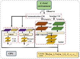
Figure 2: The proposed robust algorithm based on CDRL.

Finally, the proposed algorithm is summarized in Algorithm 1.

1 Initialize: $\kappa(\boldsymbol{s}|\eta_{1})$, $Q_{1}(\boldsymbol{s},\boldsymbol{a}|\eta_{2})$, $Q_{2}(\boldsymbol{s},\boldsymbol{a}|\eta_{2})$, $\eta_{1}^{\prime}=\eta_{1}$,$\eta_{2}^{\prime}=\eta_{2}$,$\eta_{2}^{\prime}=\eta_{2}$, $\kappa=0$, $\mathcal{M}=\emptyset$, $N_{b}=64$, $\gamma=0.5$, random Ornstein-Uhlenbeck process $\mathcal{N}$ and initial state $\boldsymbol{s}^{(0)}$.

2  Repeat: $n=n+1$.

3 $\boldsymbol{a}^{(n)}=\kappa(\boldsymbol{s}^{(n)}|\eta_{1})$.

4 $\boldsymbol{a}^{(n)}$ is selected based on (32).

5 Computing $r^{(n)}$, $c_{1}^{(n)}$ and $\boldsymbol{s}^{(n+1)}$

6 Store the transition $(\boldsymbol{s}^{(n)},\boldsymbol{a}^{(n)},r^{(n)},c^{(n)},\boldsymbol{s}^{(n+1)})$ in $\mathcal{M}$

7 Sample a random batch of $N_{b}$ transitions from$\mathcal{M}$

8 Computing (32), (33), (34) and (35).

Updating the network parameters.

Algorithm 1 Proposed CDRL algorithm for (26)

V-C Computation Complexity Analysis

Denote $N_{1}$ as the maximal number of convolutional layers, $N_{2}$ as the maximal number of input and output feature maps, and $N_{3}$ as the maximal side length of the filters in convolutional neural networks (CNN). $N_{4}$ and $N_{5}$ as the maximal number of neurons in the hidden layers and the number of hidden layers in fully-connected networks(FCN). Then the complexity in the forward pass of the actor-network in online deployment is $\mathcal{O}(N_{1}(NBU+NMB)N_{3}^{2}N_{2}^{2}+N_{5}^{2}N_{4})$[35, 36].

VI Numerical Results

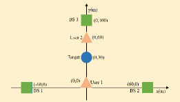
Figure 3: Simulation setup of the MA-enabled C-ISAC system.

In the simulation, the positions of the BSs, users, and targets are shown in Fig.3, where $B=3$, $U=2$, and $T=1$. Each BS is equipped with $N=8$ MAs and $M=4$ receive MAs, where $N_{x}=4$, $N_{y}=2$, $M_{x}=2$, and $M_{y}=2$. The channel path loss is modeled as $PL(d)=PL_{0}(d/d_{0})^{-\Omega}$, where $PL_{0}$ denotes the path loss factor, $d_{0}$ represents the reference distance, $d$ indicates the link distance, and $\Omega$ represents the path loss, with $PL_{0}=-30$ dB, $d_{0}=1$ m. The number of channel paths is $L_{b,u}=3$. The noise power level is $-120$ dBm. The minimum distance between MAs is set to $D=\lambda/2$. The transmission range of the MAs is $x_{t,b}^{min}=-2\lambda$, $x_{t,b}^{max}=2\lambda$, and $y_{t,b}^{min}=-2\lambda$. The range for the receive MAs is $x_{r,b}^{min}=-2\lambda$, $x_{r,b}^{max}=2\lambda$, and $y_{r,b}^{min}=-2\lambda$, $y_{r,b}^{max}=2\lambda$. The path loss exponent for the BS-user link is set to $2.8$, while the path loss exponent for the BS-target link is set to $2.2$. The target’s radar cross section (RCS) is given as $\alpha=10$. Sensing accuracy $\gamma_{b}=0.05$, and communication rate $\gamma_{b}=2$ bit/s/Hz

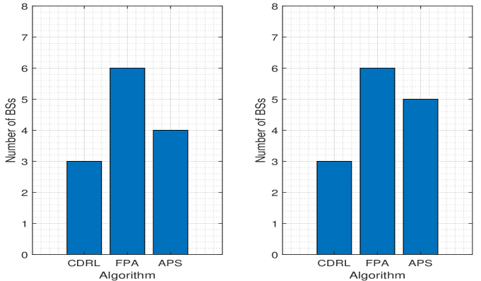
Figure 4: (a) Cumulative reward of the CDRL versus epochs. (b) Cumulative cost of the CDRL versus epochs.

We validate the proposed scheme in Fig.4 by examining the cumulative reward and cost achieved by the agent during training. In the experiment, we set the TS error to $\sigma_{\xi}=100$ ns and $\bar{\epsilon}_{b,u}=0.01$. As the training progresses, the cumulative reward increases, indicating that the agent learns to optimize its strategy to meet the system’s goals. Meanwhile, the BS adjusts its behavior to reduce the cumulative cost while satisfying both the communication rate and sensing accuracy constraints. As training continues, the agent refines its decision-making, reducing the cumulative cost below the threshold, demonstrating that the agent can find a near-optimal solution without exhaustive search. By adjusting its policy, the agent balances reward and cost, optimizing performance under the system’s constraints. As shown in Fig.4(a), despite the presence of TS and CSI errors, the reward values of the CDRL algorithm decrease slightly but remain close to those of the three alternative schemes. This indicates that, even in the intermediate stages before the policy fully converges, the algorithm can maintain a high level of stability and robustness. The reason for this lies in the robust optimization design of the CDRL algorithm, which incorporates worst-case communication rate constraints. This design enables the algorithm to perform well in the presence of environmental errors and effectively mitigates the negative impact of errors. Therefore, even when errors are present and the policy has not fully converged, the CDRL algorithm still demonstrates high robustness and stability. Additionally, Fig.4(b) shows that TS and CSI errors cause a significant increase in cumulative cost and a decrease in cumulative reward. These errors require more resources to meet the constraints, increasing the number of episodes needed for convergence.

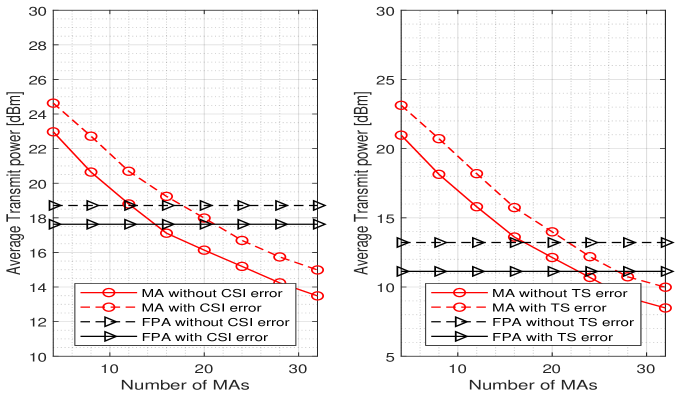
Figure 5: (a) Average transmit power versus the number of MAs with CSI error. (b) Average transmit power versus the number of MAs with TS error.

As shown in Fig.5, the simulation investigates the relationship between the number of MAs and the system’s transmit power. The results indicate that as the number of MAs increases, the system’s transmit power decreases. This is because additional MAs enhance the system’s spatial diversity performance. By increasing the number of antennas, the simulation models the signal reception process under various channel environments and finds that multiple antennas at different locations receiving signals can effectively mitigate multipath effects. By adjusting the antenna positions and utilizing beamforming techniques, the system can enhance signal directionality and suppress interference, ensuring good communication quality and target tracking accuracy under lower transmit power. The simulation results show that under the same power consumption when there is a CSI error, only $16$ MAs are required to achieve an FPA of $32$. This indicates that the number of MAs can not only reduce power consumption but also lower the BS cost. When TS errors are present, only $20$ MAs are needed to achieve an FPA of $32$, demonstrating that a small number of MAs can effectively resist TS errors. The above simulation results suggest that as the number of MAs increases, the system can meet the communication robustness requirements with lower power consumption, achieving both energy savings and resource optimization.

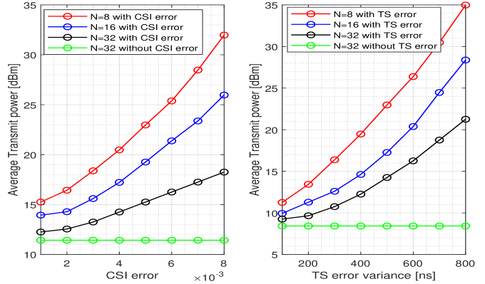
Figure 6: (a) Average transmit power versus the CSI error. (b) Average transmit power versus the TS error.

In Fig.6(a), we illustrate the relationship between the transmit power and the CSI error. It can be observed that as the CSI error increases, the transmit power of the system increases significantly. This is because CSI error reduces the accuracy of the channel state information, which in turn degrades the quality of the receive signal, leading to a decrease in SINR. To compensate for the reduction in SINR, the system must increase the transmit power to enhance the signal strength, thereby ensuring sufficient signal quality to overcome noise and interference, and maintaining the reliability of the communication link as well as the accuracy of target tracking. By increasing the transmit power, the system effectively improves SINR, reduces the estimation bias caused by CSI errors, and ensures the system can maintain high performance. In Fig.6(b), we demonstrate the relationship between the consumed power and the TS error under the same parameter settings as in Fig.6(a). Power consumption with a TS error is significantly higher than without, and the gap increases as the TS error grows. This is because TS errors force the system to consume more power to meet the HCRLB constraint, which minimizes estimation error for optimal performance. As TS error increases, uncertainty in the system’s estimation grows, requiring more power to maintain reliable and accurate tracking. The receive signal becomes more distorted, reducing the accuracy of target state estimation. To compensate for this loss in precision, the system invests additional power to boost signal strength, reducing estimation bias caused by TS errors and ensuring high performance under the HCRLB constraint. Therefore, as TS error increases, power consumption rises, reflecting the extra resources needed for high-precision tracking in the face of growing estimation errors.

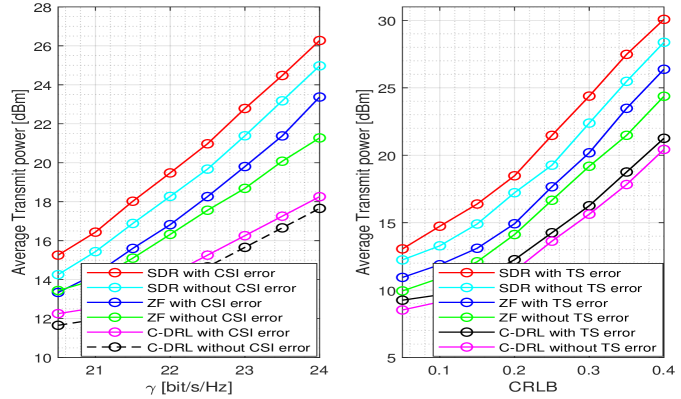
Figure 7: (a) Average transmit power versus the communication rate constraint with proposed algorithm and nonrobust algorithms. (b) Average transmit power versus the HCRLB constraint with proposed algorithm and nonrobust algorithms.

Finally, to further validate the performance of the proposed coordinated transmission beamforming algorithm under different communication rates, this section compares it with existing beamforming methods based on semidefinite relaxation (SDR) and zero-forcing (ZF). Fig.7(a) illustrates the relationship between transmit power, communication rate, and sensing accuracy under the conditions of $\sigma_{\xi}=100$ ns and $\bar{\epsilon}_{b,u}=0.01$. The simulation results show that as the communication rate increases, the system’s transmit power also increases. This is because higher communication rates require stronger signal strength to maintain a sufficient SINR that satisfies the communication demand. Additionally, the simulation results indicate that, under poor CSI conditions, the proposed robust design achieves better performance in increasing the communication rate while keeping power consumption lower compared to both the SDR and ZF-based methods. To further investigate the relationship between transmit power and HCRLB constraints, Fig.7(b) shows the correlation between transmit power and HCRLB constraints. The results indicate that as the HCRLB constraint becomes more stringent, the system’s transmit power increases significantly. This is because a stricter HCRLB constraint requires more precise target state estimation, thus demanding higher power to meet the more stringent sensing accuracy requirements. Conversely, as the HCRLB constraint is relaxed, the system’s transmit power decreases, while still being able to satisfy less strict estimation requirements with lower power. The simulation results further demonstrate that, in the presence of TS errors, the proposed robust design adapts better to different HCRLB constraints compared to the non-robust design, thereby reducing power consumption while maintaining other system performance. Furthermore, it outperforms both SDR- and ZF-based methods in terms of power efficiency and performance.

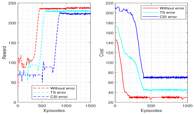
Figure 8: (a) BS selection versus the proposed algorithm and existing algorithms with $\bar{\epsilon}_{b,u}=0.01$ and $\sigma_{\xi}=100$ ns. (b) BS selection versus the proposed algorithm and existing algorithms with $\bar{\epsilon}_{b,u}=0.01$ and $\sigma_{\xi}=200$ ns.

Based on the results shown in simulation Fig. 8(a), this paper compares three schemes: the CDRL scheme, the Adaptive Portable Antenna (APS) scheme, and the FPA scheme, with a CSI error of $0.01$ in the simulation. The results show that, under a $100$ ns synchronization error, the CDRL scheme achieves the desired performance with only $3$ BSs, while the APS scheme needs $4$ BSs and the FPA scheme requires $6$ BSs. This demonstrates the CDRL scheme’s strong adaptability and lower BS requirements, achieving the same performance with fewer resources. The CDRL scheme optimizes MAs, allowing flexible adjustment of antenna positions and beamforming, improving signal diversity and mitigating errors. In contrast, the APS scheme, though using MAs, is less flexible and requires more BSs to maintain accuracy. The FPA scheme, with fixed antennas, cannot adjust dynamically and needs more BSs to ensure performance under error conditions. In Fig. 8.(b), when the synchronization error increases to $200$ ns, the CDRL scheme still only requires $3$ BSs, while the APS scheme requires $5$ BSs, and the FPA scheme still requires $6$ BSs. This confirms the superiority of the CDRL scheme, especially when synchronization errors are large. The CDRL scheme effectively mitigates the impact of these errors, keeping BS demand low. This is due to its flexibility, which leverages MAs to maintain low BS requirements under varying error conditions. In contrast, while the APS scheme also uses MAs, its error tolerance is weaker, requiring more BSs to compensate for performance loss. The FPA scheme, with its fixed antenna configuration, cannot adjust dynamically and relies on adding more BSs to maintain performance, especially under large errors. In conclusion, the CDRL scheme outperforms others by reducing BSs, cutting power consumption, and ensuring high robustness and efficiency in error-prone environments.

VII Conclusion

This paper investigates the performance of a C-ISAC network, where distributed BSs coordinate beamforming for user communication while simultaneously performing static target sensing. We have addressed the challenges introduced by imperfect CSI and TS errors, which degrade system performance. To improve robustness, we have proposed the use of MAs, which can enhance the system’s resilience to these errors. Through the analysis of CSI and TS errors, we have derived models for the worst-case achievable rate and sensing precision. To reduce power consumption, we have optimized beamforming, MA position, and BS selection, ensuring that the system meets the required performance under these errors. The optimization problem, being non-convex, has been tackled using a constrained C-DRL approach, incorporating a tailored DDPG algorithm with Wolpertinger architecture. Simulation results have shown that our proposed method significantly improves system robustness and outperforms traditional fixed-antenna systems. Future work will explore the integration of dynamic environmental factors, such as user mobility and varying interference conditions, into the optimization process. Additionally, the use of advanced machine learning algorithms to further optimize MA-aided C-ISAC systems will be investigated, aiming for even greater performance improvements in real-world scenarios.

Appendix A The proof of Theorem 1

The communication rate constraint in (13) can be rewritten as

$$\sum\nolimits_{b=1}^{B}|c_{b,u}(\hat{\boldsymbol{h}}_{b,u}(\tilde{\boldsymbol{t}}_{b})+\Delta\boldsymbol{h}_{b,u})^{H}\boldsymbol{w}_{b,u}|^{2}/\left(\sum\nolimits_{b=1}^{B}\sum\nolimits_{u^{\prime}=1,u^{\prime}\neq u}^{U}\right.$$

$$\left.\left.|c_{b,u^{\prime}}(\hat{\boldsymbol{h}}_{b,u^{\prime}}(\tilde{\boldsymbol{t}}_{b})+\Delta\boldsymbol{h}_{b,u^{\prime}})^{H}\boldsymbol{w}_{b,u^{\prime}}|^{2}\right)+\sigma_{b}^{2}\right)\geq 2^{\gamma_{u}}-1.$$ (36)

The constraint in (36) is further expressed as

$$\sum\nolimits_{b=1}^{B}|c_{b,u}(\hat{\boldsymbol{h}}_{b,u}(\tilde{\boldsymbol{t}}_{b})+\Delta\boldsymbol{h}_{b,u})^{H}\boldsymbol{w}_{b,u}|^{2}\geq(2^{\gamma_{u}}-1)\left(\sum\nolimits_{b=1}^{B}\right.$$

$$\left.\left.\sum\nolimits_{u^{\prime}=1,u^{\prime}\neq u}^{U}|c_{b,u^{\prime}}(\hat{\boldsymbol{h}}_{b,u^{\prime}}(\tilde{\boldsymbol{t}}_{b})+\Delta\boldsymbol{h}_{b,u^{\prime}})^{H}\boldsymbol{w}_{b,u^{\prime}}|^{2}\right)+\sigma_{b}^{2}\right).$$ (37)

According to the triangle inequality, we have

$$|c_{b,u}(\hat{\boldsymbol{h}}_{b,u}(\tilde{\boldsymbol{t}}_{b})+\Delta\boldsymbol{h}_{b,u})^{H}\boldsymbol{w}_{b,u}|\leq c_{b,u}|\hat{\boldsymbol{h}}_{b,u}^{H}(\tilde{\boldsymbol{t}}_{b})\boldsymbol{w}_{b,u}|+c_{b,u}|\Delta\boldsymbol{h}_{b,u}^{H}$$

$$\times\boldsymbol{w}_{b,u}|,|c_{b,u}(\hat{\boldsymbol{h}}_{b,u}(\tilde{\boldsymbol{t}}_{b})+\Delta\boldsymbol{h}_{b,u})^{H}\boldsymbol{w}_{b,u}|\geq c_{b,u}|\hat{\boldsymbol{h}}_{b,u}^{H}(\tilde{\boldsymbol{t}}_{b})\boldsymbol{w}_{b,u}|-$$

$$c_{b,u}|\Delta\boldsymbol{h}_{b,u}^{H}\boldsymbol{w}_{b,u}|,$$ (38)

Thus, based on (38), we can scale expression (37) as

$$\sum\nolimits_{b=1}^{B}(c_{b,u}|\hat{\boldsymbol{h}}_{b,u}^{H}(\tilde{\boldsymbol{t}}_{b})\boldsymbol{w}_{b,u}|-c_{b,u}|\Delta\boldsymbol{h}_{b,u}^{H}\boldsymbol{w}_{b,u}|)^{2}\geq(2^{\gamma_{u}}-1)\left(\sum\nolimits_{b=1}^{B}\right.$$

$$\left.\left.\sum\nolimits_{u^{\prime}=1,u^{\prime}\neq u}^{U}(c_{b,u^{\prime}}|\hat{\boldsymbol{h}}_{b,u^{\prime}}^{H}(\tilde{\boldsymbol{t}}_{b})\boldsymbol{w}_{b,u^{\prime}}|+c_{b,u^{\prime}}|\Delta\boldsymbol{h}_{b,u^{\prime}}^{H}\boldsymbol{w}_{b,u^{\prime}}|)^{2}\right)+\sigma_{b}^{2}\right).$$ (39)

Therefore, the left hand side of (39) is denoted as

$$\sum\nolimits_{b=1}^{B}(c_{b,u}|\hat{\boldsymbol{h}}_{b,u}^{H}(\tilde{\boldsymbol{t}}_{b})\boldsymbol{w}_{b,u}|-c_{b,u}|\Delta\boldsymbol{h}_{b,u}^{H}\boldsymbol{w}_{b,u}|)^{2}=\sum\nolimits_{b=1}^{B}(c_{b,u}\times$$

$$|\hat{\boldsymbol{h}}_{b,u}^{H}(\tilde{\boldsymbol{t}}_{b})\boldsymbol{w}_{b,u}|)^{2}+(c_{b,u}|\Delta\boldsymbol{h}_{b,u}^{H}\boldsymbol{w}_{b,u}|)^{2}-2c_{b,u}^{2}|\hat{\boldsymbol{h}}_{b,u}^{H}(\tilde{\boldsymbol{t}}_{b})\boldsymbol{w}_{b,u}||\Delta\boldsymbol{h}_{b,u}^{H}\boldsymbol{w}_{b,u}|$$

$$\geq\sum\nolimits_{b=1}^{B}(c_{b,u}|\hat{\boldsymbol{h}}_{b,u}^{H}(\tilde{\boldsymbol{t}}_{b})\boldsymbol{w}_{b,u}|)^{2}-(c_{b,u}|\Delta\boldsymbol{h}_{b,u}^{H}\boldsymbol{w}_{b,u}|)^{2}-2c_{b,u}^{2}\times$$

$$|\hat{\boldsymbol{h}}_{b,u}^{H}(\tilde{\boldsymbol{t}}_{b})\boldsymbol{w}_{b,u}||\Delta\boldsymbol{h}_{b,u}^{H}\boldsymbol{w}_{b,u}|.$$ (40)

Similarly, the right hand side of (39) is denoted as

$$(2^{\gamma_{u}}-1)\left(\sum\nolimits_{b=1}^{B}\right.\sum\nolimits_{u^{\prime}=1,u^{\prime}\neq u}^{U}(c_{b,u^{\prime}}|\hat{\boldsymbol{h}}_{b,u^{\prime}}^{H}(\tilde{\boldsymbol{t}}_{b})\boldsymbol{w}_{b,u^{\prime}}|)^{2}+(c_{b,u}\times$$

$$\left.\left.|\Delta\boldsymbol{h}_{b,u^{\prime}}^{H}\boldsymbol{w}_{b,u^{\prime}}|)^{2}+2c_{b,u^{\prime}}^{2}|\hat{\boldsymbol{h}}_{b,u^{\prime}}^{H}(\tilde{\boldsymbol{t}}_{b})\boldsymbol{w}_{b,u^{\prime}}||\Delta\boldsymbol{h}_{b,u^{\prime}}^{H}\boldsymbol{w}_{b,u^{\prime}}|\right)+\sigma_{b}^{2}\right).$$ (41)

To obtain worst-case communication rate constraint, we further rewritten (39) as (42) at the top of this page, then we use the Cauchy-Schwarz inequality to obtain the lower bound of (40) and the upper bound of (41), the constraint in (39) is finally given in (42).

$$\sum\nolimits_{b=1}^{B}(c_{b,u}|\hat{\boldsymbol{h}}_{b,u}^{H}(\tilde{\boldsymbol{t}}_{b})\boldsymbol{w}_{b,u}|)^{2}-(c_{b,u}|\Delta\boldsymbol{h}_{b,u}^{H}\boldsymbol{w}_{b,u}|)^{2}-2c_{b,u}^{2}|\hat{\boldsymbol{h}}_{b,u}^{H}(\tilde{\boldsymbol{t}}_{b})\boldsymbol{w}_{b,u}||\Delta\boldsymbol{h}_{b,u}^{H}\boldsymbol{w}_{b,u}|\geq(2^{\gamma_{u}}-1)\left(\sum\nolimits_{b=1}^{B}\right.\sum\nolimits_{u^{\prime}=1,u^{\prime}\neq u}^{U}(c_{b,u^{\prime}}|\hat{\boldsymbol{h}}_{b,u^{\prime}}^{H}(\tilde{\boldsymbol{t}}_{b})$$

$$\boldsymbol{w}_{b,u^{\prime}}|)^{2}+\left.\left.(c_{b,u}|\Delta\boldsymbol{h}_{b,u^{\prime}}^{H}\boldsymbol{w}_{b,u^{\prime}}|)^{2}+2c_{b,u^{\prime}}^{2}|\hat{\boldsymbol{h}}_{b,u^{\prime}}^{H}(\tilde{\boldsymbol{t}}_{b})\boldsymbol{w}_{b,u^{\prime}}||\Delta\boldsymbol{h}_{b,u^{\prime}}^{H}\boldsymbol{w}_{b,u^{\prime}}|\right)+\sigma_{b}^{2}\right)\xlongequal{\textrm{Cauchy-Schwarz Inequality}|\Delta\boldsymbol{h}_{b,u}^{H}\boldsymbol{w}_{b,u}|^{2}\leq\|\Delta\boldsymbol{h}_{b,u}\|^{2}\|\boldsymbol{w}_{b,u}\|^{2}}\sum\nolimits_{b=1}$$

$$(c_{b,u}|\hat{\boldsymbol{h}}_{b,u}^{H}(\tilde{\boldsymbol{t}}_{b})\boldsymbol{w}_{b,u}|)^{2}-(c_{b,u}\|\Delta\boldsymbol{h}_{b,u}\|^{2}|\boldsymbol{w}_{b,u}|^{2})-2c_{b,u}^{2}|\hat{\boldsymbol{h}}_{b,u}^{H}(\tilde{\boldsymbol{t}}_{b})\boldsymbol{w}_{b,u}|\sqrt{\|\Delta\boldsymbol{h}_{b,u}\|^{2}\|\boldsymbol{w}_{b,u}\|^{2}}\geq(2^{\gamma_{u}}-1)\left(\sum\nolimits_{b=1}^{B}\right.\sum\nolimits_{u^{\prime}=1,u^{\prime}\neq u}^{U}(c_{b,u^{\prime}}|$$

$$\hat{\boldsymbol{h}}_{b,u^{\prime}}^{H}(\tilde{\boldsymbol{t}}_{b})\boldsymbol{w}_{b,u^{\prime}}|)^{2}+c_{b,u}^{2}\|\Delta\boldsymbol{h}_{b,u^{\prime}}\|^{2}\left.\left.\times\|\boldsymbol{w}_{b,u^{\prime}}\|^{2}+2c_{b,u^{\prime}}^{2}|\hat{\boldsymbol{h}}_{b,u^{\prime}}^{H}(\tilde{\boldsymbol{t}}_{b})\boldsymbol{w}_{b,u^{\prime}}|\sqrt{\|\Delta\boldsymbol{h}_{b,u^{\prime}}\|^{2}\|\boldsymbol{w}_{b,u^{\prime}}\|^{2}}\right)+\sigma_{b}^{2}\right).$$ (42)

However, since $\epsilon_{b,u}$ is unknown, we consider how to determine $\epsilon_{b,u}$. Next, we address $\|\Delta\boldsymbol{h}_{b,u}\|$ in equation (42), and we have

$$\hat{\boldsymbol{h}}_{b,u}=\hat{\boldsymbol{A}}_{b,u}(\tilde{\boldsymbol{t}})(\hat{\tilde{\boldsymbol{h}}}_{b,u}+\Delta\tilde{\boldsymbol{h}}_{b,u})=$$

$$\left[\begin{matrix}e^{j2\pi/\lambda(x_{1}^{b}\sin(\hat{\theta}_{1}^{b}+\Delta\theta_{1}^{b})\cos(\hat{\phi}_{1}^{b}+\Delta\phi_{1}^{b})+y_{1}^{b}\cos(\hat{\theta}_{1}^{b}+\Delta\theta_{1}^{b}))}&\cdots&e^{j2\pi/\lambda(x_{1}^{b}\sin(\hat{\theta}_{L_{b,u}}^{b}+\Delta\theta_{L_{b,u}}^{b})\cos(\hat{\phi}_{L_{b,u}}^{b}+\Delta\phi_{L_{b,u}}^{b})+y_{1}^{b}\cos(\hat{\theta}_{L_{b,u}}^{b}+\Delta\theta_{L_{b,u}}^{b}))}\\ \vdots&\ddots&\vdots\\ e^{j2\pi/\lambda(x_{N}^{b}\sin(\hat{\theta}_{1}^{b}+\Delta\theta_{1}^{b})\cos(\hat{\phi}_{1}^{b}+\Delta\phi_{1}^{b})+y_{N}^{b}\cos(\hat{\theta}_{1}^{b}+\Delta\theta_{1}^{b}))}&\cdots&e^{j2\pi/\lambda(x_{N}^{b}\sin(\hat{\theta}_{L_{b,u}}^{b}+\Delta\theta_{L_{b,u}}^{b})\cos(\hat{\phi}_{L_{b,u}}^{b}+\Delta\phi_{L_{b,u}}^{b})+y_{N}^{b}\cos(\hat{\theta}_{L_{b,u}}^{b}+\Delta\theta_{L_{b,u}}^{b}))}\\ \end{matrix}\right]$$

$$\times\left[\hat{\tilde{h}}_{b,u,1}+\Delta\tilde{h}_{b,u,1},\cdots,\hat{\tilde{h}}_{b,u,L_{b,u}}+\Delta\tilde{h}_{b,u,L_{b,u}}\right]^{T}.$$ (43)

Then, $\|\Delta\boldsymbol{h}_{b,u}\|^{2}$ is rewritten as

$$|\Delta\boldsymbol{h}_{b,u}|^{2}=|\hat{\boldsymbol{h}}_{b,u}(\tilde{\boldsymbol{t}}_{b})-\boldsymbol{h}_{b,u}(\tilde{\boldsymbol{t}}_{b})|^{2}=\sum\nolimits_{n=1}^{N}|\sum\nolimits_{i=1}^{L_{b,u}}$$

$$e^{j2\pi/\lambda(x_{t,b}^{n}\sin(\hat{\theta}_{i}^{b}+\Delta\theta_{i}^{b})\cos(\hat{\phi}_{i}^{b}+\Delta\phi_{i}^{b})+y_{t,b}^{n}\cos(\hat{\theta}_{i}^{b}+\Delta\theta_{i}^{b})\sin(\hat{\phi}_{i}^{b}+\Delta\phi_{i}^{b}))}$$

$$(\hat{\tilde{h}}_{b,u,i}+\Delta\tilde{h}_{b,u,i})-e^{j2\pi/\lambda(x_{j}^{b}\sin(\hat{\theta}_{i}^{b})\cos(\hat{\phi}_{i}^{b})+y_{j}^{b}\cos(\hat{\theta}_{i}^{b})\sin(\hat{\phi}_{i}^{b}))}\hat{\tilde{h}}_{b,u,i}|^{2}.$$ (44)

Then, we can use the first order Taylor series of $\sin(\hat{\theta}_{i}^{b}+\Delta\theta_{i}^{b})=\sin(\hat{\theta}_{i}^{b})+\Delta\theta_{i}^{b}\cos(\hat{\theta}_{i}^{b})$ and $\cos(\hat{\theta}_{i}^{b}+\Delta\theta_{i}^{b})=\cos(\hat{\theta}_{i}^{b})-\Delta\theta_{i}^{b}\sin(\hat{\theta}_{i}^{b})$ to obtain

$$\sum_{j=1}^{N}|\sum\nolimits_{i=1}^{L_{b,u}}e^{j2\pi/\lambda(x_{j}^{b}(-\Delta\phi_{i}^{b}\sin(\hat{\phi}_{i}^{b})\sin(\hat{\theta}_{t}^{b})+\Delta\theta_{i}^{b}\cos(\hat{\phi}_{i}^{b})\cos(\hat{\theta}_{t}^{b}))}$$

$$e^{j2\pi/\lambda-x_{j}^{b}(\Delta\phi_{i}^{b}\Delta\theta_{i}^{b}\sin(\hat{\phi}_{i}^{b})\cos(\hat{\theta}_{i}^{b}))-y_{j}^{b}\Delta\theta_{i}^{b}\sin(\hat{\theta}_{i}^{b})))}(\hat{\tilde{h}}_{b,u,i}+\Delta\tilde{h}_{b,u,i})$$

$$+e^{j2\pi/\lambda(x_{j}^{b}\sin(\hat{\theta}_{i}^{b})\cos(\hat{\phi}_{i}^{b})+y_{j}^{b}\cos(\hat{\theta}_{i}^{b}))}\Delta\tilde{h}_{b,u,i}|^{2}.$$ (45)

Then, by applying the triangle inequality, we can further enlarge the result to obtain the upper bound of $|\Delta\boldsymbol{h}_{b,u}|^{2}$, and the upper bound is given in (46) at the top of next page.

$$\sum\nolimits_{j=1}^{N}|\sum\nolimits_{i=1}^{L_{b,u}}e^{j2\pi/\lambda(x_{j}^{b}(-\Delta\phi_{i}^{b}\sin(\hat{\phi}_{i}^{b})\sin(\hat{\theta}_{t}^{b})+\Delta\theta_{i}^{b}\cos(\hat{\phi}_{i}^{b})\cos(\hat{\theta}_{t}^{b}))}e^{j2\pi/\lambda-x_{j}^{b}(\Delta\phi_{i}^{b}\Delta\theta_{i}^{b}\sin(\hat{\phi}_{i}^{b})\cos(\hat{\theta}_{i}^{b}))-y_{j}^{b}\Delta\theta_{i}^{b}\sin(\hat{\theta}_{i}^{b})))}(\hat{\tilde{h}}_{b,u,i}+\Delta\tilde{h}_{b,u,i})|^{2}$$

$$+|\sum\nolimits_{i=1}^{L_{b,u}}e^{j2\pi/\lambda(x_{j}^{b}\sin(\hat{\theta}_{i}^{b})\cos(\hat{\phi}_{i}^{b})+y_{j}^{b}\cos(\hat{\theta}_{i}^{b}))}\Delta\tilde{h}_{b,u,i}|^{2}\leq\sum\nolimits_{j=1}^{N}|\sum\nolimits_{i=1}^{L_{b,u}}e^{j2\pi/\lambda(x_{j}^{b}(-\Delta\phi_{i}^{b}\sin(\hat{\phi}_{i}^{b})\sin(\hat{\theta}_{t}^{b})+\Delta\theta_{i}^{b}\cos(\hat{\phi}_{i}^{b})\cos(\hat{\theta}_{t}^{b}))}$$

$$e^{j2\pi/\lambda-x_{j}^{b}(\Delta\phi_{i}^{b}\Delta\theta_{i}^{b}\sin(\hat{\phi}_{i}^{b})\cos(\hat{\theta}_{i}^{b}))-y_{j}^{b}\Delta\theta_{i}^{b}\sin(\hat{\theta}_{i}^{b})))}\hat{\tilde{h}}_{b,u,i}|^{2}+2NL_{b,u}\epsilon_{b,u}=N\|\hat{\tilde{\boldsymbol{h}}}_{b,u,i}\|^{2}+2NL_{b,u}\bar{\epsilon}_{b,u}.$$ (46)

Therefore, the upper bound of $|\Delta\boldsymbol{h}_{b,u}|^{2}$ is expressed as

$$|\Delta\boldsymbol{h}_{b,u}|^{2}\leq N\|\hat{\tilde{\boldsymbol{h}}}_{b,u}\|^{2}+2NL_{b,u}\bar{\epsilon}_{b,u}.$$ (47)

Finally, by substituting the results from (47) into equation (42), we obtain the worst-case communication rate constraint, and it is given in (15). The Theorem 1 is proofed in Appendix A

Appendix B The proof of (23)

As stated in [30], the $(o_{1},o_{2})$-th entry of the OFIM and PFIM is expressed as, respectively

$$\boldsymbol{\Xi}^{o}_{b}[o_{1},o_{2}]=-\mathbb{E}\left(\frac{\partial^{2}\ln p(\tilde{\boldsymbol{y}}_{b};\boldsymbol{\zeta}_{b})}{\partial\boldsymbol{\zeta}_{b}[o_{1}]\partial\boldsymbol{\zeta}_{b}[o_{2}]}\right)$$

$$=\frac{2}{\sigma_{b}^{2}}\mathrm{Re}\left\{\frac{\partial\tilde{\boldsymbol{x}}_{b}^{H}}{\partial\boldsymbol{\zeta}_{b}[o_{1}]}\frac{\partial\tilde{\boldsymbol{x}}_{b}}{\partial\boldsymbol{\zeta}_{b}[o_{2}]}\right\}+\underbrace{\mathrm{Tr}\left(\boldsymbol{I}_{b}^{-1}\frac{\partial\boldsymbol{I}_{b}}{\partial\boldsymbol{\zeta}_{b}[o_{1}]}\boldsymbol{I}_{b}^{-1}\frac{\partial\boldsymbol{I}_{b}}{\partial\boldsymbol{\zeta}_{b}[o_{2}]}\right)}_{\boldsymbol{0}}$$

$$=\frac{2}{\sigma_{b}^{2}}\mathrm{Re}\left\{\frac{\partial\tilde{\boldsymbol{x}}_{b}^{H}}{\partial\boldsymbol{\zeta}_{b}[o_{1}]}\frac{\partial\tilde{\boldsymbol{x}}_{b}}{\partial\boldsymbol{\zeta}_{b}[o_{2}]}\right\}$$ (48)

and

$$\boldsymbol{\Xi}^{p}_{b}[o_{1},o_{2}]=-\mathbb{E}\left(\frac{\partial^{2}\ln p(\Delta\boldsymbol{\xi}_{b})}{\partial\boldsymbol{\zeta}_{b}[o_{1}]\partial\boldsymbol{\zeta}_{b}[o_{2}]}\right)$$

$$=\frac{2}{\sigma_{\xi}^{2}}\mathrm{Re}\left\{\frac{\partial\Delta\boldsymbol{\xi}_{b}^{H}}{\partial\boldsymbol{\zeta}_{b}[o_{1}]}\frac{\partial\Delta\boldsymbol{\xi}_{b}}{\partial\boldsymbol{\zeta}_{b}[o_{2}]}\right\}+\underbrace{\mathrm{Tr}\left(\boldsymbol{I}_{b}^{-1}\frac{\partial\boldsymbol{I}_{b}}{\partial\boldsymbol{\zeta}_{b}[o_{1}]}\boldsymbol{I}_{b}^{-1}\frac{\partial\boldsymbol{I}_{b}}{\partial\boldsymbol{\zeta}_{b}[o_{2}]}\right)}_{\boldsymbol{0}}$$

$$=\frac{2}{\sigma_{\xi}^{2}}\mathrm{Re}\left\{\frac{\partial\Delta\boldsymbol{\xi}_{b}^{H}}{\partial\boldsymbol{\zeta}_{b}[o_{1}]}\frac{\partial\Delta\boldsymbol{\xi}_{b}}{\partial\boldsymbol{\zeta}_{b}[o_{2}]}\right\},$$ (49)

in which $\boldsymbol{\zeta}_{b}[o_{1}]$ and $\boldsymbol{\zeta}_{b}[o_{1}]$ are the $o_{1}$-th element and $o_{2}$-th element of $\boldsymbol{\zeta}_{b}$, respectively. In (48) and (49), we observe that to determine the expressions of (48) and (49), it is necessary to compute the derivatives of $\tilde{\boldsymbol{x}}_{b}$ and $\Delta\boldsymbol{\xi}_{b}$ to the unknown parameter $\boldsymbol{\zeta}_{b}$. Specifically, based on (17), the derivatives of $\tilde{\boldsymbol{x}}_{b}$ and $\Delta\boldsymbol{\xi}_{b}$ with respect to $x_{T}$ are expressed as follows:

$$\frac{\partial\tilde{\boldsymbol{x}}_{b}}{\partial x_{T}}=\sum\nolimits_{b^{\prime}=1}^{B}\frac{\partial\mathrm{vec}(\boldsymbol{H}_{b,b^{\prime}}(\tilde{\boldsymbol{r}}_{b^{\prime}},\tilde{\boldsymbol{t}}_{b})\boldsymbol{\Omega}_{b})}{\partial x_{T}}+\frac{\partial\hat{\xi}_{b,b^{\prime}}^{p}}{\partial x_{T}}\times$$

$$\mathrm{vec}(\boldsymbol{H}_{b,b^{\prime}}(\tilde{\boldsymbol{r}}_{b^{\prime}},\tilde{\boldsymbol{t}}_{b})\bar{\boldsymbol{\Omega}}_{b}),~\frac{\partial\tilde{\boldsymbol{\xi}}_{b}}{\partial x_{T}}=\boldsymbol{0},$$ (50)

in which $\boldsymbol{\Omega}_{b}=[\bar{c}_{b}\boldsymbol{W}_{b}e^{-jf_{1}\hat{\xi}_{b,b^{\prime}}^{p}}\boldsymbol{s}_{b}(f_{1}),\cdots,\bar{c}_{b}\boldsymbol{W}_{b}e^{-jf_{\bar{S}}\hat{\xi}_{b,b^{\prime}}^{p}}\\ \boldsymbol{s}_{b}(f_{\bar{S}})]$ and $\bar{\boldsymbol{\Omega}}_{b}=[-jf_{1}\bar{c}_{b}\boldsymbol{W}_{b}e^{-jf_{1}\hat{\xi}_{b,b^{\prime}}^{p}}\boldsymbol{s}_{b}(f_{1}),\cdots,-jf_{M}\bar{c}_{b}\\ \boldsymbol{W}_{b}e^{-jf_{\bar{S}}\hat{\xi}_{b,b^{\prime}}^{p}}\boldsymbol{s}_{b}(f_{\bar{S}})]$. According to vectorization rules $\frac{\partial\mathrm{vec}(\boldsymbol{A}\boldsymbol{B})}{\partial x}=\mathrm{vec}(\frac{\partial\boldsymbol{A}}{\partial x}\boldsymbol{B})$ in[37]. Thus, we can determine the expression for A after computing the derivative of $\boldsymbol{H}_{b,b^{\prime}}(\tilde{\boldsymbol{r}}_{b^{\prime}},\tilde{\boldsymbol{t}}_{b})$ and $\tau_{b,b^{\prime}}$ with respect to $x_{T}$, i.e.,

$$\frac{\partial\boldsymbol{H}(\tilde{\boldsymbol{r}}_{b^{\prime}},\tilde{\boldsymbol{t}}_{b})}{\partial x_{T}}=\alpha_{b,b^{\prime}}\frac{\partial\boldsymbol{a}(\tilde{\boldsymbol{r}}_{b^{\prime}})}{\partial x_{T}}\boldsymbol{a}(\tilde{\boldsymbol{t}}_{b})^{H}+\alpha_{b,b^{\prime}}\boldsymbol{a}(\tilde{\boldsymbol{r}}_{b^{\prime}})\frac{\partial\boldsymbol{a}(\tilde{\boldsymbol{t}}_{b})}{\partial x_{T}}^{H}$$ (51)

$$\frac{\partial\tau_{b,b^{\prime}}}{\partial x_{T}}=1/c(x_{T}-x_{b})/v_{b}+(x_{T}-x_{b^{\prime}})/v_{b^{\prime}}).$$ (52)

According to the chain rule of differentiation[37], $\frac{\partial\boldsymbol{a}(\tilde{\boldsymbol{r}}_{b^{\prime}})}{\partial x_{T}}$ and $\frac{\partial\boldsymbol{a}(\tilde{\boldsymbol{t}}_{b})}{\partial x_{T}}$ are given by

$$\frac{\partial\boldsymbol{a}(\tilde{\boldsymbol{r}}_{b^{\prime}})}{\partial x_{T}}=\left(\frac{\partial\rho^{b^{\prime}}(\boldsymbol{r}_{b^{\prime}}^{m})}{\partial\bar{\theta}_{b}}\frac{\partial\bar{\theta}_{b}}{x_{T}}+\frac{\partial\rho^{b^{\prime}}(\boldsymbol{r}_{b^{\prime}}^{m})}{\partial\bar{\phi}_{b}}\frac{\partial\bar{\phi}_{b}}{x_{T}}\right)\bar{\boldsymbol{a}}(\tilde{\boldsymbol{r}}_{b^{\prime}})\odot\boldsymbol{a}(\tilde{\boldsymbol{r}}_{b^{\prime}})$$

$$\frac{\partial\boldsymbol{a}(\tilde{\boldsymbol{t}}_{b})}{\partial x_{T}}=\left(\frac{\partial\rho^{b}(\boldsymbol{t}_{b}^{n})}{\partial\theta_{b}}\frac{\partial\theta_{b}}{x_{T}}+\frac{\partial\rho^{b}(\boldsymbol{t}_{b}^{n})}{\partial\phi_{b}}\frac{\partial\phi_{b}}{x_{T}}\right)\bar{\boldsymbol{a}}(\tilde{\boldsymbol{t}}_{b})\odot\boldsymbol{a}(\tilde{\boldsymbol{t}}_{b}),$$ (53)

where $\bar{\boldsymbol{a}}(\tilde{\boldsymbol{r}}_{b^{\prime}})=[j2\pi/\lambda\rho_{1}(\boldsymbol{t}),\cdots,j2\pi/\lambda\rho_{N}(\boldsymbol{t})]$ and $\bar{\boldsymbol{a}}(\tilde{\boldsymbol{r}}_{b^{\prime}})=[j2\pi/\lambda\rho_{1}(\boldsymbol{t}),\cdots,j2\pi/\lambda\rho_{N}(\boldsymbol{t})]$. Moreover, $\frac{\partial\rho^{b}(\boldsymbol{t}_{b}^{n})}{\partial\theta_{b}}$, $\frac{\partial\rho^{b}(\boldsymbol{t}_{b}^{n})}{\partial\phi_{b}}$, $\frac{\partial\rho^{b^{\prime}}(\boldsymbol{r}_{b^{\prime}}^{m})}{\partial\bar{\theta}_{b}}$ and $\frac{\partial\rho^{b^{\prime}}(\boldsymbol{r}_{b^{\prime}}^{m})}{\partial\bar{\phi}_{b}}$ are expressed as

$$\frac{\partial\rho^{b}(\boldsymbol{t}_{b}^{n})}{\partial\theta_{b}}=x_{n}^{b}\cos\theta^{b}\cos\phi^{b}-y_{n}^{b}\sin\theta^{b},$$

$$\frac{\partial\rho^{b^{\prime}}(\boldsymbol{r}_{b^{\prime}}^{m})}{\partial\bar{\theta}_{b}}=x_{m}^{b}\cos\theta^{b}\cos\phi^{b}-y_{m}^{b}\sin\theta^{b},$$

$$\frac{\partial\rho^{b}(\boldsymbol{t}_{b}^{n})}{\partial\phi_{b}}=-x_{n}^{b}\sin\theta^{b}\sin\phi^{b},\frac{\partial\rho^{b^{\prime}}(\boldsymbol{r}_{b^{\prime}}^{m})}{\partial\bar{\phi}_{b}}=-x_{m}^{b}\sin\theta^{b}\sin\phi^{b},$$ (54)

$\frac{\partial\theta_{b}}{\partial x_{T}}$, $\frac{\partial\phi_{b}}{\partial x_{T}}$, $\frac{\partial\bar{\theta}_{b^{\prime}}}{\partial x_{T}}$ and $\frac{\partial\bar{\phi}_{b^{\prime}}}{\partial x_{T}}$ are given at the top of this page.

$$\frac{\partial\theta_{b}}{\partial x_{T}}=\frac{y_{b}-x_{b}}{(x_{T}-y_{b})^{2}+(x_{T}-x_{b})^{2}},~\frac{\partial\phi_{b}}{\partial x_{T}}=-\frac{z_{b}\cdot\left((x_{T}-x_{b})+(x_{T}-y_{b})\right)}{(x_{T}-x_{b})^{2}+(x_{T}-y_{b})^{2}+z_{b}^{2}\cdot((x_{T}-x_{b})^{2}+(x_{T}-y_{b})^{2})},$$

$$\frac{\partial\bar{\theta}_{b^{\prime}}}{\partial x_{T}}=\frac{y_{b}^{\prime}-x_{b}^{\prime}}{(x_{T}-y_{b}^{\prime})^{2}+(x_{T}-x_{b}^{\prime})^{2}},~\frac{\partial\bar{\phi}_{b^{\prime}}}{\partial x_{T}}=-\frac{z_{b}^{\prime}\cdot\left((x_{T}-x_{b}^{\prime})+(x_{T}-y_{b}^{\prime})\right)}{(x_{T}-x_{b}^{\prime})^{2}+(x_{T}-y_{b}^{\prime})^{2}+(z_{b}^{\prime})^{2}\cdot((x_{T}-x_{b}^{\prime})^{2}+(x_{T}-y_{b}^{\prime})^{2})},$$ (55)

Similarly, we can determine the derivative of $\boldsymbol{H}_{b,b^{\prime}}(\tilde{\boldsymbol{r}}_{b^{\prime}},\tilde{\boldsymbol{t}}_{b})$ and $\tau_{b,b^{\prime}}$ with respect to $y_{T}$. The derivative of $\tilde{\boldsymbol{x}}_{b}$ with respect to $\Delta\boldsymbol{\xi}_{b}[o_{3}]$ is expressed as

$$\frac{\partial\tilde{\boldsymbol{x}}_{b}}{\partial\Delta\boldsymbol{\xi}_{b}[o_{3}]}=\mathrm{vec}(\boldsymbol{H}_{b,b^{\prime}}\bar{\boldsymbol{\Omega}}_{b}),$$ (56)

in which $\Delta\boldsymbol{\xi}_{b}[o_{3}]$ is the $o_{3}$-th element of $\Delta\boldsymbol{\xi}_{b}$. Then, $\frac{\partial^{2}p(\tilde{\boldsymbol{y}}_{b};\boldsymbol{\zeta}_{b})}{\partial\boldsymbol{\zeta}_{b}[o_{1}]\partial\boldsymbol{\zeta}_{b}[o_{2}]}$ can be further specifically expressed as

$$\frac{\partial^{2}p(\tilde{\boldsymbol{y}}_{b};\boldsymbol{\zeta}_{b})}{\partial\boldsymbol{\zeta}_{b}[o_{1}]\partial\boldsymbol{\zeta}_{b}[o_{2}]}=\left[\begin{matrix}\frac{\partial^{2}p(\tilde{\boldsymbol{y}}_{b};\boldsymbol{\zeta}_{b})}{\partial x_{T}\partial x_{T}}&\frac{\partial^{2}p(\tilde{\boldsymbol{y}}_{b};\boldsymbol{\zeta}_{b})}{\partial x_{T}\partial y_{T}}&\frac{\partial^{2}p(\tilde{\boldsymbol{y}}_{b};\boldsymbol{\zeta}_{b})}{\partial x_{T}\partial\Delta\boldsymbol{\xi}_{b}}\\ \frac{\partial^{2}p(\tilde{\boldsymbol{y}}_{b};\boldsymbol{\zeta}_{b})}{\partial y_{T}\partial x_{T}}&\frac{\partial^{2}p(\tilde{\boldsymbol{y}}_{b};\boldsymbol{\zeta}_{b})}{\partial y_{T}\partial y_{T}}&\frac{\partial^{2}p(\tilde{\boldsymbol{y}}_{b};\boldsymbol{\zeta}_{b})}{\partial y_{T}\partial\Delta\boldsymbol{\xi}_{b}}\\ \frac{\partial^{2}p(\tilde{\boldsymbol{y}}_{b};\boldsymbol{\zeta}_{b})}{\partial x_{T}\partial\Delta\boldsymbol{\xi}_{b}}&\frac{\partial^{2}p(\tilde{\boldsymbol{y}}_{b};\boldsymbol{\zeta}_{b})}{\partial y_{T}\partial\Delta\boldsymbol{\xi}_{b}}&\frac{\partial^{2}p(\tilde{\boldsymbol{y}}_{b};\boldsymbol{\zeta}_{b})}{\partial\Delta\boldsymbol{\xi}_{b}\partial\Delta\boldsymbol{\xi}_{b}}\end{matrix}\right].$$ (57)

Based on (48) and (49), $\frac{\partial^{2}p(\tilde{\boldsymbol{y}}_{b};\boldsymbol{\zeta}_{b})}{\partial x_{T}\partial x_{T}}$ is computed as (58) at the top of next page.

$$\frac{\partial^{2}p(\tilde{\boldsymbol{y}}_{b};\boldsymbol{\zeta}_{b})}{\partial x_{T}\partial x_{T}}=\frac{2}{\sigma_{b}^{2}}\mathrm{Re}\left\{\left(\sum\nolimits_{b^{\prime}=1}^{B}\frac{\partial\mathrm{vec}(\boldsymbol{H}_{b,b^{\prime}}(\tilde{\boldsymbol{r}}_{b^{\prime}},\tilde{\boldsymbol{t}}_{b})\boldsymbol{\Omega}_{b})}{\partial x_{T}}+\frac{\partial\hat{\xi}_{b,b^{\prime}}^{p}}{\partial x_{T}}\mathrm{vec}(\boldsymbol{H}_{b,b^{\prime}}(\tilde{\boldsymbol{r}}_{b^{\prime}},\tilde{\boldsymbol{t}}_{b})\bar{\boldsymbol{\Omega}}_{b})\right)^{H}\left(\sum\nolimits_{b^{\prime}=1}^{B}\frac{\partial\mathrm{vec}(\boldsymbol{H}_{b,b^{\prime}}(\tilde{\boldsymbol{r}}_{b^{\prime}},\tilde{\boldsymbol{t}}_{b})\boldsymbol{\Omega}_{b})}{\partial x_{T}}+\right.\right.$$

$$\left.\left.\frac{\partial\hat{\xi}_{b,b^{\prime}}^{p}}{\partial x_{T}}\mathrm{vec}(\boldsymbol{H}_{b,b^{\prime}}(\tilde{\boldsymbol{r}}_{b^{\prime}},\tilde{\boldsymbol{t}}_{b})\bar{\boldsymbol{\Omega}}_{b})\right)\right\}=\frac{2}{\sigma_{b}^{2}}\mathrm{Re}\left\{\sum\nolimits_{m=1}^{M}\mathrm{Tr}\left(\sum\nolimits_{s=1}^{\bar{S}}|\boldsymbol{s}_{b}(f_{s})|^{2}\left(\frac{\partial\boldsymbol{H}(\tilde{\boldsymbol{r}}_{b^{\prime}},\tilde{\boldsymbol{t}}_{b})}{\partial x_{T}}-jf_{s}\frac{\partial\tau_{b,b^{\prime}}}{\partial x_{T}}\boldsymbol{H}(\tilde{\boldsymbol{r}}_{b^{\prime}},\tilde{\boldsymbol{t}}_{b})\right)^{H}\left(\frac{\partial\boldsymbol{H}(\tilde{\boldsymbol{r}}_{b^{\prime}},\tilde{\boldsymbol{t}}_{b})}{\partial x_{T}}-\right.\right.\right.$$

$$\left.\left.jf_{s}\frac{\partial\tau_{b,b^{\prime}}}{\partial x_{T}}\boldsymbol{H}(\tilde{\boldsymbol{r}}_{b^{\prime}},\tilde{\boldsymbol{t}}_{b}))\boldsymbol{w}\boldsymbol{w}^{H}\right)\right\}.$$ (58)

Similarly, $\frac{\partial^{2}p(\tilde{\boldsymbol{y}}_{b};\boldsymbol{\zeta}_{b})}{\partial x_{T}\partial x_{T}}$ and $\frac{\partial^{2}p(\tilde{\boldsymbol{y}}_{b};\boldsymbol{\zeta}_{b})}{\partial x_{T}\partial x_{T}}$ are denoted as (59) at the top of next page.

$$\frac{\partial^{2}p(\tilde{\boldsymbol{y}}_{b};\boldsymbol{\zeta}_{b})}{\partial x_{T}\partial y_{T}}=\frac{2}{\sigma_{b}^{2}}\mathrm{Re}\left\{\sum_{m=1}^{M}\mathrm{Tr}\left(\sum_{s=1}^{\bar{S}}|\boldsymbol{s}_{b}(f_{s})|^{2}\left(\frac{\partial\boldsymbol{H}(\tilde{\boldsymbol{r}}_{b^{\prime}},\tilde{\boldsymbol{t}}_{b})}{\partial x_{T}}-jf_{s}\frac{\partial\tau_{b,b^{\prime}}}{\partial x_{T}}\boldsymbol{H}(\tilde{\boldsymbol{r}}_{b^{\prime}},\tilde{\boldsymbol{t}}_{b})\right)^{H}\left(\frac{\partial\boldsymbol{H}(\tilde{\boldsymbol{r}}_{b^{\prime}},\tilde{\boldsymbol{t}}_{b})}{\partial y_{T}}-jf_{s}\frac{\partial\tau_{b,b^{\prime}}}{\partial y_{T}}\boldsymbol{H}(\tilde{\boldsymbol{r}}_{b^{\prime}},\tilde{\boldsymbol{t}}_{b})\right)\boldsymbol{w}\boldsymbol{w}^{H}\right)\right\},$$

$$\frac{\partial^{2}p(\tilde{\boldsymbol{y}}_{b};\boldsymbol{\zeta}_{b})}{\partial y_{T}\partial x_{T}}=\frac{2}{\sigma_{b}^{2}}\mathrm{Re}\left\{\sum_{m=1}^{M}\mathrm{Tr}\left(\sum_{s=1}^{\bar{S}}|\boldsymbol{s}_{b}(f_{s})|^{2}\left(\frac{\partial\boldsymbol{H}(\tilde{\boldsymbol{r}}_{b^{\prime}},\tilde{\boldsymbol{t}}_{b})}{\partial y_{T}}-jf_{s}\frac{\partial\tau_{b,b^{\prime}}}{\partial y_{T}}\boldsymbol{H}(\tilde{\boldsymbol{r}}_{b^{\prime}},\tilde{\boldsymbol{t}}_{b})\right)^{H}\left(\frac{\partial\boldsymbol{H}(\tilde{\boldsymbol{r}}_{b^{\prime}},\tilde{\boldsymbol{t}}_{b})}{\partial x_{T}}-jf_{s}\frac{\partial\tau_{b,b^{\prime}}}{\partial x_{T}}\boldsymbol{H}(\tilde{\boldsymbol{r}}_{b^{\prime}},\tilde{\boldsymbol{t}}_{b})\right)\boldsymbol{w}\boldsymbol{w}^{H}\right)\right\}.$$ (59)

Similarly, according to (58) and (59), $\frac{\partial^{2}p(\tilde{\boldsymbol{y}}_{b};\boldsymbol{\zeta}_{b})}{\partial x_{T}\partial\Delta\boldsymbol{\xi}_{b}}$ and $\frac{\partial^{2}p(\tilde{\boldsymbol{y}}_{b};\boldsymbol{\zeta}_{b})}{\partial x_{T}\partial\Delta\boldsymbol{\xi}_{b}}$ are given by (60) at the top of next page.

$$\frac{\partial^{2}p(\tilde{\boldsymbol{y}}_{b};\boldsymbol{\zeta}_{b})}{\partial x_{T}\partial\Delta\boldsymbol{\xi}_{b}}=\frac{2}{\sigma_{b}^{2}}\mathrm{Re}\left\{\sum_{m=1}^{M}\mathrm{Tr}\left(\sum\nolimits_{s=1}^{\bar{S}}|\boldsymbol{s}_{b}(f_{s})|^{2}\left(\frac{\partial\boldsymbol{H}(\tilde{\boldsymbol{r}}_{b^{\prime}},\tilde{\boldsymbol{t}}_{b})}{\partial x_{T}}-jf_{s}\frac{\partial\tau_{b,b^{\prime}}}{\partial x_{T}}\boldsymbol{H}(\tilde{\boldsymbol{r}}_{b^{\prime}},\tilde{\boldsymbol{t}}_{b})\right)^{H}\boldsymbol{H}(\tilde{\boldsymbol{r}}_{b^{\prime}},\tilde{\boldsymbol{t}}_{b})\boldsymbol{w}\boldsymbol{w}^{H}\right)\right\},$$

$$\frac{\partial^{2}p(\tilde{\boldsymbol{y}}_{b};\boldsymbol{\zeta}_{b})}{\partial y_{T}\partial\Delta\boldsymbol{\xi}_{b}}=\frac{2}{\sigma_{b}^{2}}\mathrm{Re}\left\{\sum_{m=1}^{M}\mathrm{Tr}\left(\sum\nolimits_{s=1}^{\bar{S}}|\boldsymbol{s}_{b}(f_{s})|^{2}\left(\frac{\partial\boldsymbol{H}(\tilde{\boldsymbol{r}}_{b^{\prime}},\tilde{\boldsymbol{t}}_{b})}{\partial y_{T}}-jf_{s}\frac{\partial\tau_{b,b^{\prime}}}{\partial y_{T}}\boldsymbol{H}(\tilde{\boldsymbol{r}}_{b^{\prime}},\tilde{\boldsymbol{t}}_{b})\right)^{H}\boldsymbol{H}(\tilde{\boldsymbol{r}}_{b^{\prime}},\tilde{\boldsymbol{t}}_{b})\boldsymbol{w}\boldsymbol{w}^{H}\right)\right\}.$$ (60)

Then, when $o_{3}\neq o_{3}^{\prime}$, $\frac{\partial^{2}p(\tilde{\boldsymbol{y}}_{b};\boldsymbol{\zeta}_{b})}{\partial\Delta\boldsymbol{\xi}_{b}[o_{3}]\partial\Delta\boldsymbol{\xi}_{b}[o_{3}]}=0$, when $o_{3}=o_{3}^{\prime}$, $\frac{\partial^{2}p(\tilde{\boldsymbol{y}}_{b};\boldsymbol{\zeta}_{b})}{\partial\Delta\boldsymbol{\xi}_{b}[o_{3}]\partial\Delta\boldsymbol{\xi}_{b}[o_{3}]}$ is expressed as

$$\frac{\partial^{2}p(\tilde{\boldsymbol{y}}_{b};\boldsymbol{\zeta}_{b})}{\partial\Delta\boldsymbol{\xi}_{b}[o_{3}]\partial\Delta\boldsymbol{\xi}_{b}[o_{3}]}=\frac{2}{\sigma_{b}^{2}}\mathrm{Re}\{\sum\nolimits_{m=1}^{M}\mathrm{Tr}(\sum\nolimits_{s=1}^{\bar{S}}f_{s}^{2}|\boldsymbol{s}_{b}(f_{s})|^{2}$$

$$\boldsymbol{H}(\tilde{\boldsymbol{r}}_{b^{\prime}},\tilde{\boldsymbol{t}}_{b})^{H}\boldsymbol{H}(\tilde{\boldsymbol{r}}_{b^{\prime}},\tilde{\boldsymbol{t}}_{b})\boldsymbol{w}\boldsymbol{w}^{H})\}.$$ (61)

Finally, we focus on $\frac{\partial^{2}p(\Delta\boldsymbol{\xi}_{b})}{\partial\boldsymbol{\zeta}_{b}\partial\boldsymbol{\zeta}_{b}}$, and the extended expression of $\frac{\partial^{2}p(\Delta\boldsymbol{\xi}_{b})}{\partial\boldsymbol{\zeta}_{b}\partial\boldsymbol{\zeta}_{b}}$ is expressed as

$$\frac{\partial^{2}p(\Delta\boldsymbol{\xi}_{b})}{\partial\boldsymbol{\zeta}_{b}\partial\boldsymbol{\zeta}_{b}}=\left[\begin{matrix}\frac{\partial^{2}p(\Delta\boldsymbol{\xi}_{b})}{\partial x_{T}\partial x_{T}}&\frac{\partial^{2}p(\Delta\boldsymbol{\xi}_{b})}{\partial x_{T}\partial x_{T}}&\frac{\partial^{2}p(\Delta\boldsymbol{\xi}_{b})}{\partial x_{T}\partial\Delta\boldsymbol{\xi}_{b}}\\ \frac{\partial^{2}p(\Delta\boldsymbol{\xi}_{b})}{\partial x_{T}\partial x_{T}}&\frac{\partial^{2}p(\Delta\boldsymbol{\xi}_{b})}{\partial x_{T}\partial x_{T}}&\frac{\partial^{2}p(\Delta\boldsymbol{\xi}_{b})}{\partial x_{T}\partial\Delta\boldsymbol{\xi}_{b}}\\ \frac{\partial^{2}p(\Delta\boldsymbol{\xi}_{b})}{\partial x_{T}\partial\Delta\boldsymbol{\xi}_{b}}&\frac{\partial^{2}p(\Delta\boldsymbol{\xi}_{b})}{\partial x_{T}\partial x_{T}}&\frac{\partial^{2}p(\Delta\boldsymbol{\xi}_{b})}{\partial\Delta\boldsymbol{\xi}_{b}\partial\Delta\boldsymbol{\xi}_{b}}\end{matrix}\right].$$ (62)

Since $p(\Delta\boldsymbol{\xi}_{b})$ and $x_{T}$ and $y_{T}$ are uncorrelated, we have

$$\frac{\partial^{2}p(\Delta\boldsymbol{\xi}_{b})}{\partial x_{T}\partial x_{T}}=0,\frac{\partial^{2}p(\Delta\boldsymbol{\xi}_{b})}{\partial y_{T}\partial y_{T}}=0,\frac{\partial^{2}p(\Delta\boldsymbol{\xi}_{b})}{\partial x_{T}\partial\Delta\boldsymbol{\xi}_{b}}=\boldsymbol{0}$$

$$\frac{\partial^{2}p(\Delta\boldsymbol{\xi}_{b})}{\partial y_{T}\partial x_{T}}=0,\frac{\partial^{2}p(\Delta\boldsymbol{\xi}_{b})}{\partial y_{T}\partial\Delta\boldsymbol{\xi}_{b}}=\boldsymbol{0}.$$ (63)

Then, $\frac{\partial^{2}p(\Delta\boldsymbol{\xi}_{b})}{\partial\Delta\boldsymbol{\xi}_{b}\partial\Delta\boldsymbol{\xi}_{b}}$ is denoted as

$$\frac{\partial^{2}p(\Delta\boldsymbol{\xi}_{b})}{\partial\Delta\boldsymbol{\xi}_{b}\partial\Delta\boldsymbol{\xi}_{b}}=\frac{1}{\sigma_{b}^{2}}\frac{\partial\Delta\boldsymbol{\xi}_{b}^{T}}{\partial\Delta\boldsymbol{\xi}_{b}}\boldsymbol{\Sigma}_{\Delta}^{-1}\frac{\partial\Delta\boldsymbol{\xi}_{b}}{\partial\Delta\boldsymbol{\xi}_{b^{\prime}}}=\boldsymbol{I}.$$ (64)

Thus, we have $\frac{\partial^{2}p(\Delta\boldsymbol{\xi}_{b})}{\partial\Delta\boldsymbol{\xi}_{b}\partial\Delta\boldsymbol{\xi}_{b}}=\boldsymbol{I}$.

References

- [1] D. C. Nguyen, M. Ding, P. N. Pathirana, A. Seneviratne, J. Li, D. Niyato, O. Dobre, and H. V. Poor, “6G internet of things: A comprehensive survey,” IEEE Internet Things J., vol. 9, no. 1, pp. 359–383, 2022.
- [2] N. Gonz´alez-Prelcic, M. Furkan Keskin, O. Kaltiokallio, M. Valkama, D. Dardari, X. Shen, Y. Shen, M. Bayraktar, and H. Wymeersch, “The integrated sensing and communication revolution for 6G: Vision, techniques, and applications,” Proc. IEEE, vol. 112, no. 7, pp. 676–723, 2024.
- [3] Y. Cui, F. Liu, X. Jing, and J. Mu, “Integrating sensing and communi- cations for ubiquitous IoT: Applications, trends, and challenges,” IEEE Network, vol. 35, no. 5, pp. 158–167, 2021.
- [4] F. Liu, Y.-F. Liu, A. Li, C. Masouros, and Y. C. Eldar, “Cram´er-rao bound optimization for joint radar-communication beamforming,” IEEE Trans. Signal Process., vol. 70, pp. 240–253, 2022.
- [5] L. Leyva, D. Castanheira, A. Silva, and A. Gameiro, “Hybrid beamform- ing design for communication-centric ISAC,” IEEE Sens. J., vol. 24, no. 13, pp. 21 179–21 190, 2024.
- [6] Z. Yu, X. Hu, C. Liu, M. Peng, and C. Zhong, “Location sensing and beamforming design for IRS-enabled multi-user ISAC systems,” IEEE Trans. Signal Process., vol. 70, pp. 5178–5193, 2022.
- [7] X. Gan, C. Huang, Z. Yang, X. Chen, J. He, Z. Zhang, C. Yuen, Y. Liang Guan, and M. Debbah, “Coverage and rate analysis for integrated sensing and communication networks,” IEEE J. Sel. Areas Commun., vol. 42, no. 9, pp. 2213–2227, 2024.
- [8] X. Yang, Z. Wei, J. Xu, Y. Fang, H. Wu, and Z. Feng, “Coordinated transmit beamforming for networked ISAC with imperfect CSI and time synchronization,” IEEE Trans. Wireless Commun., pp. 1–1, 2024.
- [9] H. Pilaram, M. Kiamari, and B. H. Khalaj, “Distributed synchronization and beamforming in uplink relay asynchronous OFDMA CoMP net- works,” IEEE Trans. Wireless Commun., vol. 14, no. 6, pp. 3471–3480, 2015.
- [10] W. Sun, E. G. Str¨om, F. Br¨annstr¨om, and M. R. Gholami, “Random broadcast based distributed consensus clock synchronization for mobile networks,” IEEE Trans. Wireless Commun., vol. 14, no. 6, pp. 3378– 3389, 2015.
- [11] R. D. Preuss and D. R. Brown, III, “Two-way synchronization for co- ordinated multicell retrodirective downlink beamforming,” IEEE Trans. Signal Process., vol. 59, no. 11, pp. 5415–5427, 2011.
- [12] D. Xu, X. Yu, D. W. K. Ng, A. Schmeink, and R. Schober, “Robust and secure resource allocation for ISAC systems: A novel optimiza- tion framework for variable-length snapshots,” IEEE Trans. Commun., vol. 70, no. 12, pp. 8196–8214, 2022.
- [13] Y. Xu, N. Cao, Y. Jin, H. Zhang, C. Huang, Q. Chen, and C. Yuen, “Robust beamforming design for integrated sensing and communication systems,” IEEE J. Sel. Areas Sensor., vol. 1, pp. 114–123, 2024.
- [14] G. Cheng, Y. Fang, J. Xu, and D. W. K. Ng, “Optimal coordinated transmit beamforming for networked integrated sensing and communi- cations,” IEEE Trans. Wireless Commun., vol. 23, no. 8, pp. 8200–8214, 2024.
- [15] L. Zhou, J. Yao, M. Jin, T. Wu, and K.-K. Wong, “Fluid antenna-assisted ISAC systems,” IEEE Wireless Commun. Lett., vol. 13, no. 12, pp. 3533– 3537, 2024.
- [16] C. Wang, G. Li, H. Zhang, K.-K. Wong, Z. Li, D. W. K. Ng, and C.-B. Chae, “Fluid antenna system liberating multiuser MIMO for ISAC via deep reinforcement learning,” IEEE Trans. Wireless Commun., vol. 23, no. 9, pp. 10 879–10 894, 2024.
- [17] H. Qin, W. Chen, Q. Wu, Z. Zhang, Z. Li, and N. Cheng, “Cram´er-rao bound minimization for movable antenna-assisted multiuser integrated sensing and communications,” IEEE Wireless Commun. Lett., vol. 13, no. 12, pp. 3404–3408, 2024.
- [18] W. Liu, X. Zhang, H. Xing, J. Ren, Y. Shen, and S. Cui, “UAV-enabled wireless networks with movable-antenna array: Flexible beamforming and trajectory design,” IEEE Wireless Commun. Lett., pp. 1–1, 2024.
- [19] Y. Xiu, Y. Zhao, R. Yang, H. Tang, L. Qu, M. Khabbaz, C. Assi, and N. Wei, “Latency minimization for movable antennas-enabled relay- aided d2d mobile edge computing communication systems,” arXiv preprint arXiv:2412.11351, 2024.
- [20] G. Hu, Q. Wu, D. Xu, K. Xu, J. Si, Y. Cai, and N. Al-Dhahir, “Movable antennas-assisted secure transmission without eavesdroppers’ instantaneous CSI,” IEEE Trans. Mob. Comput., vol. 23, no. 12, pp. 14 263–14 279, 2024.
- [21] Y. Xiu, Y. Zhao, S. Yang, M. Xu, D. Niyato, Y. Li, and N. Wei, “Delay minimization for movable antennas-enabled anti-jamming communica- tions with mobile edge computing,” arXiv preprint arXiv:2409.14418, 2024.
- [22] D. Dash and V. Jayaraman, “A probabilistic model for sensor fusion using range-only measurements in multistatic radar,” IEEE Sensors Letters, vol. 4, no. 6, pp. 1–4, 2020.
- [23] L. Zhu, W. Ma, and R. Zhang, “Movable-antenna array enhanced beam- forming: Achieving full array gain with null steering,” IEEE Commun. Lett., vol. 27, no. 12, pp. 3340–3344, Oct. 2023.
- [24] S. Yang, W. Lyu, B. Ning, Z. Zhang, and C. Yuen, “Flexible precoding for multi-user movable antenna communications,” IEEE Wireless Com- mun. Lett., vol. 13, no. 5, pp. 1404–1408, Mar. 2024.
- [25] B. Li, H. Zeng, X. Zhu, Y. Jiang, and Y. Wang, “Cooperative time syn- chronization and robust clock parameters estimation for time-sensitive cell-free massive MIMO systems,” IEEE Trans. Wireless Commun., vol. 23, no. 9, pp. 11 552–11 566, 2024.
- [26] F. Lu, G. Liu, W. Lu, Y. Gao, J. Cao, N. Zhao, and A. Nallanathan, “Resource and trajectory optimization for UAV-relay-assisted secure maritime MEC,” IEEE Trans. Commun., vol. 72, no. 3, pp. 1641–1652, Nov. 2024.
- [27] L. Zhu, W. Ma, and R. Zhang, “Modeling and performance analysis for movable antenna enabled wireless communications,” IEEE Trans. Wireless Commun., vol. 23, no. 6, pp. 6234–6250, Nov. 2024.
- [28] Y. Xiu, Y. Zhao, S. Yang, Y. Zhang, D. Niyato, H. Du, and N. Wei, “Robust beamforming design for near-field DMA-NOMA mmwave communications with imperfect position information,” IEEE Trans. Wireless Commun., pp. 1–1, 2024.
- [29] Z. Xiao, S. Cao, L. Zhu, Y. Liu, B. Ning, X.-G. Xia, and R. Zhang, “Channel estimation for movable antenna communication systems: A framework based on compressed sensing,” IEEE Trans. Wireless Com- mun., pp. 1–1, Apr. 2024.
- [30] Y. Noam and H. Messer, “Notes on the tightness of the hybrid Cramer–Rao lower bound,” IEEE Trans. Signal Process., vol. 57, no. 6, pp. 2074–2084, 2009.
- [31] M. Pardini, F. Lombardini, and F. Gini, “The hybrid Cramer–Rao bound on broadside DOA estimation of extended sources in presence of array errors,” IEEE Trans. Signal Process., vol. 56, no. 4, pp. 1726–1730, 2008.
- [32] H. Messer, “The hybrid Cramer-Rao lower bound - from practice to theory,” in Fourth IEEE Workshop on Sensor Array and Multichannel Processing, 2006., 2006, pp. 304–307.
- [33] Z. Wei, H. Liu, Z. Feng, H. Wu, F. Liu, Q. Zhang, and Y. Du, “Deep cooperation in ISAC system: Resource, node and infrastructure perspectives,” IEEE Internet Things Mag., vol. 7, no. 6, pp. 118–125, 2024.
- [34] T. Lillicrap, “Continuous control with deep reinforcement learning,” arXiv preprint arXiv:1509.02971, 2015.
- [35] Y. Gao, X. Yuan, D. Yang, Y. Hu, Y. Cao, and A. Schmeink, “UAV- assisted MEC system with mobile ground terminals: DRL-based joint terminal scheduling and UAV 3D trajectory design,” IEEE Trans. Veh. Technol., pp. 1–17, Mar. 2024.
- [36] Y. Ju, H. Wang, Y. Chen, T.-X. Zheng, Q. Pei, J. Yuan, and N. Al- Dhahir, “Deep reinforcement learning based joint beam allocation and relay selection in mmWave vehicular networks,” IEEE Trans. Commun., vol. 71, no. 4, pp. 1997–2012, 2023.
- [37] J. N. Franklin, Matrix theory. Courier Corporation, 2012.