Quasisteady Patterns in Interfaces: Folding and Faceting
Abstract.
We present a systematic derivation of the gradient flows associated to a broad class of interfacial energies, emphasizing the relation between intrinsic and extrinsic variations of the interface. We show that the intrinsic variables formulation brings the gradient flow into alignment with the traditional analysis of quasi-steady dynamical systems defined on a stationary domain. Gradient flows are derived for model systems which exhibit quasi-steady pattern formation including coarsening among faceted interfaces and nonlocal interactions that model membrane self-adhesion and self-avoidance.
1. Introduction
There is a rich literature describing quasi-steady pattern formation via reductive limits of activator-inhibitor and chemotactic reaction diffusion systems. Generically, these system have been posed on a fixed domain. Many applications in biological and chemical process are mediated by an evolving membrane. This includes fluid membranes, such as lipid bilayers, composed of thin layers of materials that diffuse relatively easily in the in-plane direction. The goal of this work is to present a minimal framework for the derivation of gradient flows of energies associated to interfaces as a tool for quasi-steady analysis of the evolving interface.
The local self-energy of an infinitely thin fluidic membrane does not depend upon deformation from a reference configuration but rather on its intrinsic local variables – the metric and curvatures as defined by the first and second fundamental forms. The iconic example is the Canham-Helfrich energy, [Canham (1970)]-[Helfrich (1973)], which models a two-dimensional interface embedded in through a simple quadratic dependence of the interfacial energy on the two membrane curvatures. Subject to various constraints, its -gradient flows give variants of a Willmore flow, [Rupp (2024)]. The complexity induced by the parameterization of an interface embedded in can inhibit model development and analysis of more complicated surface energies. Frameworks set in higher dimensional settings are available in the literature, [Barrett et al (2020)] but are generally geared towards computational implementation.
We present a minimal framework for the derivation of gradient flows of interfacial energies embedded in , casting them as dynamical systems of the intrinsic variables of the interface. We consider a general local energy incorporating terms up to second order in surface diffusion, and then extend this to incorporate two-point interaction kernels that describe membrane self-interactions at a distance. Throughout we emphasize how the tools from quasi-adiabatic reduction can be brought to bear upon these important classes of problems.
We present a systematic derivation of first and second variations of these energies with respect to the intrinsic coordinates. This is conducted within the framework of classical calculus of variations, with the conditions that the intrinsic coordinates generate a smoothly closed curve captured through an explicit set of constraints. The gradient flow is described as an evolution system for the intrinsic variables, highlighting the relation between the arc length variation of the energy and the first integral of the functional variation at an equilibrium. Reducing the scope to a family of energies that are first order in surface gradient of curvature, explicit relations for the second variation are extracted and their connection to the linearization of the gradient flow at equilibrium and quasi-equilibrium are investigated. As an application we introduce a faceting energy, essentially an Allen-Cahn energy in the interfacial curvature, emphasizing the parallels between this Allen-Cahn curvature gradient flow and that of the famous Cahn-Hilliard system on a fixed domain.
In Section 5, we present a class of two point energies that include adhesion-repulsion effects. These are modeled through interaction kernels that characterize the energetic cost of surface self-proximity through double surface integrals. These model electrostatic interaction at longer range and hard-core repulsion at short range, evocative of Lenard-Jones potentials. We derive expressions for their gradient flow and apply them to an energy combining a Canham-Helfrich curvature and a surface area penalty term. We show formally that the system stabilizes two points of a curve at closest approach at a prescribed distance. Surprisingly, the two-point energies induce a set of non-trivial curve-constraints associated to energy invariance under rigid body motions, as outlined in Section 7.3. Simulations of the associated gradient flow show a rich regime of quasi-steady folded states, similar to labyrinthine patterns. The gradient flow navigates these labyrinthine states to arrive at a final folded equilibrium state.
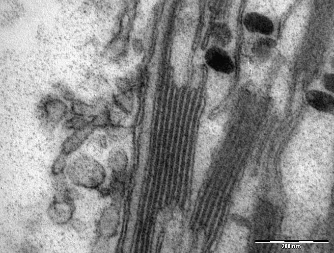
The Canham-Helfrich adhesion-repulsion energy captures stacking and folding effects commonly seen in cellular organelles, such as the Golgi apparatus [Tachikawa & Mochizuki (2017)], the endoplasmic reticulum [Shemesh et al (2014)], and thylakoid membranes that enclose the chloroplasts that conduct photosynthesis, see Figure 1 and [Austin and Staehelin (2011)]. It also has applications to folding of charged polymer chains [Tabliabue et al (2024)]. The appendix presents a discussion of the numerical scheme and technical lemmas that support the main text.
2. General Formalism for Curve Evolution
We focus on an evolving curve parameterized by a map where is the circle of unit circumference. Denoting the unit tangent vector and outward unit normal vector of the curve at the point by and respectively. We denote arc length by
| (2.1) |
In , it is natural to use the metric, defined through the first fundamental form of the surface. In using arc-length affords some simplification in the formulation, in the metric reduces to the square of the arc-length. As a minor notational point, we refer to as the arc length as a shortened version of the arc length parameterization. We normalize the gradients with arc-length as this leads to a simpler formulation, in particular surface area scales linearly with With this caveat we define the surface gradient
the Laplace-Beltrami operator
the surface measure
and the curvature
| (2.2) |
Under these definitions a circle admits a positive constant curvature. The following relations hold
| (2.3) |
The curve is uniquely defined, up to rigid body motion, by its intrinsic coordinates which maps into Here and below superscript denotes transpose of a vector in The deformation of the curve can be specified through an extrinsic vector field that establishes normal and tangential velocities, denoted . This corresponds to the evolution
| (2.4) |
The extrinsic vector field defined on induces the intrinsic vector field through the relations
| (2.5) | ||||
see [Pismen (2006)][Sec 3.4].
Denote the angle of the tangent vector to the x-axis by . It is helpful to recast the unit tangent and normal vectors and as explicit functions of :
which satisfy the trigonometric relations
| (2.6) |
where here and below denotes differentiation with respect to Since the expression for from (2.3) yields the relation
| (2.7) |
A curve is smoothly closed if its end points and tangent vectors both align at the point of periodicity of . More specifically defining the jump of a function
then a pair of -periodic curvature and arc-length corresponds to a curve with a smoothly closed images if and only if
| (2.8) | ||||
| (2.9) |
This forms the admissible class of curvature-arc length pairs that lead to smoothly closed images,
| (2.10) |
where is defined as . We set aside issues of self-intersection of the curve, these must be handled on an energy and flow dependent manner.
To understand the evolution of these jump quantities, it is instructive to take the time derivative of the first equality in (2.3). Recalling the dependence of yields
and distributing the derivatives we obtain
Taking the dot product with the normal establishes the evolution equation
| (2.11) |
Since the curvature and the velocity are -periodic it follows that
Lemma 1.
Consider a curve evolving under a prescribed -periodic extrinsic velocity If the initial curve satisfies then the jump quantities and are invariant for smooth solutions of the flow (2.5) subject to -periodic boundary conditions. In particular a curve that is initially smoothly closed will remain smoothly closed.
Proof.
From (2.11) is -periodic so that
Thus if then satisfies (2.9) for all In particular we deduce that the tangent and normal are -periodic. This allows us to integrate-by-parts in integrals involving Specifically we evaluate the time derivative of ,
Using (2.7) to replace we integrate-by-parts
The last equality follows from the identity (2.6), and the periodicity of . ∎
The first and second fundamental from evolution equations (2.5) can be written as a linear map from the extrinsic vector field to the intrinsic vector field
| (2.12) |
through the operator
| (2.13) |
Here we have introduced the surface Helmoltz operator The operator G is not strictly positive, in particular
where the pairing denote the usual inner product. The operator satisfies the identities
| (2.14) |
which allow a characterization of the kernel of
Lemma 2.
For any smooth curve the operator subject to periodic boundary conditions has a three dimensional kernel corresponding to rigid body motions of the curve,
where denote the canonical basis of
Proof.
For any fixed vector the extrinsic vector field is the infinitesimal generator of rigid translation of in the direction . The identities (2.14) and the relations (2.3) yield
The rigid body rotation of curve induced by at fixed rate about the origin induces the extrinsic velocity where J is the matrix for rotation by The G identities and the relations (2.3) again yield
However while These three vectors are linearly independent and since is a third order operator, its eigenspaces cannot be more than three dimensional, hence these vectors span the kernel. ∎
2.1. Reparameterization
The image of is denoted
The image is independent of re-parameterization of the map More specifically, let be 1-1 and continuously differentiable. Without loss of generality we may assume that , uniformly on The image of the original and reparameterized map coincide . From the chain rule
so that
In particular given an arc length it can reparameterized into a -constant via the map which solves the nonlinear ODE
subject to . The constant value of is chosen to satisfy the periodicity condition and is unique since the value increases monotonically with . This is the parameterization taken in the computations presented in Section 7.1, however in the analysis the arc length is treated generally to emphasize the structure of the systems.
Denoting then for any its reparameterized form satisfies
Similarly, under the change of variables, while the reparameterized tangent, normal and curvature satisfy the analogous forms of (2.3). In particular the energies considered in the next section are independent of parameterization. The equivalence of reparameterization and tangential extrinsic flow is established in Section 7.2 of the Appendix.
3. Critical points, Local Minima, and Gradient Flows of Local Intrinsic Energies
A local intrinsic energy depends only upon the first and second fundamental forms, specifically the curvature and arc length and their local derivatives. A generic local-intrinsic energy involving the curvature and its surface derivatives up to second order takes the form
| (3.1) |
where and is assumed to be smooth. Although the value of is independent of the choice of arc length , it appears formally in the scaling of the surface measure and of the surface differentials and in the constraints required for curve closure. We derive intrinsic and extrinsic representation for the variational derivatives of and define the associated gradient flow of subject to the closed curve constraints.
3.1. Lagrange Multiplier Formulation
The functional is defined over the admissible space comprised of smooth arc length-curvature pairs that satisfy the curve closure relations (2.8)-(2.9). Bounded energy generally does not enforce smoothness on the arc length, however the energy is invariant under reparameterization. In the time independent minimization problem for this allows one to restrict the admissible set to pairs with arc length that is constant over Nonetheless, it is instructive for the gradient flow problem to consider the perturbation problem for without imposing spatially constant arc length. We consider a general class of admissible perturbation paths
| (3.2) |
for with tangent The curve closure relations constrain these paths, so we expand both the energy and the constraint
| (3.3) | ||||
| (3.4) |
where and denote first and second -variational derivatives with respect to variations in the intrinsic coordinate . Unless otherwise indicated, all instances of correspond to its value at the perturbation point , in particular this applies to the measure associated to . Since we have and equating orders of in the expansion yields three orthogonality conditions that characterize the tangent plane
At second order in , the system places the correction term in a quadratic relation with
| (3.5) |
The function is a critical point of if and only if the coefficient of in the energy expansion is zero, equivalently for all This requires that the first variation of lies in the row space of Equivalently, critical points of satisfy the, generally elliptic, PDE
| (3.6) |
where is a Lagrange multiplier associated to the constraint. If in addition is a local minima of it is necessary that the -coefficient in the expansion be non-negative. The quadratic correction can be removed from this term via the critical point equation and the quadratic relation with That is applying first (3.6) and then (3.5) we have
| (3.7) |
The non-negativity of the coefficient of in the energy expansion is equivalent to the condition
| (3.8) |
for all We introduce the Lagrange second variational operator, associated to a critical point solving (3.6) with Lagrange multiplier ,
| (3.9) |
This corresponds to the second variation of the Lagrange multiplier energy
| (3.10) |
In the next two sections we make these calculations explicit.
3.2. Variation of the Constraints
To compute the first and second variation requires regular expansions the surface measure and surface diffusion operators. To the perturbed surface measure expands as
| (3.11) |
We introduce the differential of at with differential
| (3.12) |
so that
| (3.13) |
The inverse arc length expansion
yields the surface gradient expansion
| (3.14) |
where we introduced the operators at in differential
The first constraint condition is given in terms of the tangent angle defined through via (2.7). Its -expansion
satisfies
We introduce the operator
| (3.15) |
which inverts . From Fubini’s Theorem its adjoint takes the form
Clearly
so when acting on functions with zero mass the operator is skew adjoint Using (2.7) we match orders of in this expansion to those of . Integrating the orders of with respect to , and back substituting for , yields the relations
| (3.16) | ||||
Using the and expansions (3.11), the first closure relation admits the asymptotic form
where and . Equating orders of yields the integral conditions
| (3.17) | ||||
| (3.18) |
Replacing with its D representation and taking adjoints yields the integral condition
| (3.19) |
Using the identity the quadratic correction integral condition (3.18) takes the form
| (3.20) | ||||
We introduce the vector functions
| (3.21) | ||||
| (3.22) |
where denotes the th entry of a vector. The integral conditions can be written as projections
| (3.23) | ||||
| (3.24) |
for . Here the second variation of the constraint system is a three-tensor with entries
| (3.25) | ||||
for . For the second closure relation, expanding and the surface measure yields
Equating orders of yields the relations
| (3.26) | ||||
We introduce the vector function
| (3.27) |
and write the second closure constraint conditions as projection conditions
| (3.28) | ||||
| (3.29) |
Here the three-tensor has third entry
| (3.30) |
Proposition 3.
3.3. Variations of the Energy
Expanding the energy along the path requires expansions of , and The first two are given in (3.11) and (3.14) respectively. For the third we apply (3.14) twice
and introduce the operators
for which the surface diffusion admits the expansion
| (3.32) |
With this notation the surface diffusion of curvature admits the expansion
To illuminate the structure within this expansion we introduce the surface differential operators defined at with differential
This notation allows a compact expansion of curvature gradients
| (3.33) |
for Applying the surface differential expansions (3.33) and the surface measure expansion (3.13), to the -path energy Taylor expansion (3.3), the first variation follows from the chain rule,
| (3.34) |
Here, for , denotes the partial derivative of with respect to its dependence upon the k’th-order surface gradient . For simplicity we have used the compressed notation and for each Grouping factors of and integrating by parts yields an explicit representation for the first intrinsic variation
| (3.35) |
At a critical point the intrinsic variation is orthogonal to all To establish that a critical point is a local minimum requires non-negativity of the second variation,
The representation for the energy contribution from follows directly from the first variation (3.35), and its contribution will be replaced by the Lagrange multiplier form of the second constraint variation. The second energy variation and its quadratic dependence on is a novel quantity. It admits the expansion
| (3.36) |
where for we denote and Using (3.12) to replace and the formula (3.34) for the first variation yields
| (3.37) |
Integration by parts in the operators allows the right-hand side to be rewritten in the bilinear form presented in the left-hand side, yielding an explicit representation for the self-adjoint operator At this level of generality the exact expression is cumbersome. An explicit representation is pursued for a first-order energy in Section 3.5. At a critical point the variation satisfies (3.6) and can be replaced with the bilinear action of on the Hessian of the constraint, yielding the formal Lagrange multiplier expansion associated to (3.10)
that incorporates the impact of the curve closure constraints.
3.4. Gradient Flows
An extrinsic velocity induces an evolution in through the relation (2.12). The chain rule implies that the time derivative of the energy evaluated on the evolving satisfies the relation
| (3.38) |
where the transpose of is
and we have introduced the extrinsic variation of ,
| (3.39) |
We verify in Lemma 5 (see Section 7.2 of Appendix) that the second entry of the extrinsic variation, is zero, and the tangential velocity drops out of the energy dissipation mechanism. More specifically, denoting the th row of by we have
| (3.40) |
If is a critical point of then , and hence is independent of . This has the interpretation that the arc-length variation, , is an arc length-weighted first integral of the functional variation of and is the flip-side of the fact that tangential velocity is equivalent to reparameterization and hence does not impact the energy, see Lemma 4 in Section 7.2 of Appendix.
Remark 1.
The arc length variation can be viewed as a weighted version of the Hamiltonian that is constant along orbits corresponding to critical points of the functional variation. This structure was exploited by Alikakos and co-authors in their fixed-domain construction of heteroclinic orbits that are critical points of a multi-component Allen-Cahn energies with several global minima, [Alikakos et al (2006)], [Alikakos and Fusco (2008)]. Indeed they relate critical points of the Allen-Cahn energy to critical points of a Jacobi functional
through a geometric version of the least action principle [Giaquinta and Hildebrandt (1996)].
These calculations motivate the following definition of the gradient normal velocity of
| (3.41) |
For an arbitrary, smooth tangential velocity the gradient flow takes the form
| (3.42) |
which affords the -independent dissipation mechanism
A complete description of the gradient flow in the intrinsic coordinates requires a choice of tangential velocity. Although a tangential velocity is equivalent to a reparameterization and does not impact the system energy, it cannot be ignored within the intrinsic equation system. A common choice is the so-called “co-moving” frame, for which . A second choice is scaled arc length, for which is constant over but may not be constant in time. We remark that a constant in time and space arc-length parameterization (called fixed arc length) requires that the size of the reference domain change in time. This has the consequence that the curvature and tangential velocities are no longer -periodic, and greatly complications the formulation. Fixed arc-length is not considered here. For scaled arc-length the tangential motion satisfies
| (3.43) |
More specifically since is a spatial constant for scaled arc-length this implies that
where D is given in (3.15) and is the percentage of total curve length contained in the image of the curve restricted to From an analytical point of view the scaled arc-length tangential velocity reduces the arc length evolution to a scalar ODE, but considerably complicates the curvature evolution through the inclusion of in the right-hand side of (3.42) as a convective term. For the derivation of the linearized system we consider the co-moving gauge.
3.5. First Order Energies
We simplify the formulas for the intrinsic Hessian for a class of energies that involve surface gradients up to first order,
| (3.44) |
The representation (3.35) of the intrinsic gradient reduces to
| (3.45) |
Similarly, restricting the second variation of given in (3.36) to the first-order energy yields,
| (3.46) | ||||
Factoring out the terms with and integrating by parts we deduce that
| (3.47) |
The entry of is the linearization of with respect to , which we denote by Similarly, denoting by the linearization of with respect to , we have the self-adjoint form
| (3.48) |
Together with the expressions (3.25) and (3.30) for , the result (3.47) yields an explicit formulation for the constrained second variation defined in (3.9).
The normal velocity associated to the first-order energy of the form (3.44) takes the form
| (3.49) |
As an example, the first order energy (3.44) includes the classical Canham-Helfrich energy as a special case. The Canham-Helfrich energy has no surface diffusion term and a quadratic curvature dependence with even parity, reducing the energy density to . The associated Canham-Helfrich normal velocity recovers the classical Willmore flow with a dependent mean curvature
| (3.50) |
The gradient flow associated to (3.44) can be written in the form (3.42), however for an equilibrium analysis it is illustrative to separate out both prefactors of , writing the flow as
| (3.51) |
subject to periodic boundary conditions on At a general point the linearization of the right-hand side yields a complicated operator. However at an equilibrium the relations allow the linearization to be significantly simplified. The first simplification arises from the fact that the variation of and drop out since they act on the zero term The second simplification arises from using the equilibrium equations to rewrite the entry, which allows the and terms to be identified as adjoints of each other. The result is the anticipated linearization
| (3.52) |
with taking the equilibrium form (3.48). For a general the self-adjoint geometric prefactor takes the form
Since , with a maximal three dimensional kernel, it has a non-negative square root , with a three dimensional kernel corresponding to rigid body motions of the underlying interface. At an equilibrium the operator is a product of a non-negative, self-adjoint operator and a self-adjoint operator. This is evocative of the structure exploited in the spectral analysis of the quasi-steady states of the Cahn-Hilliard equation, [Chen 2007]. While a comprehensive analysis of the spectrum of is an open problem, the kernel of is amenable to symmetry. For an equilibrium we act with the infinitesimal generator of translations, , on the critical point equation to obtain
from which we infer the translational element of the kernel of the Hessian,
| (3.53) |
4. Application: Faceting Energy
To investigate quasi-adiabatic dynamics in a gradient flow, we consider a “faceting energy” within the first-order framework (3.44) with
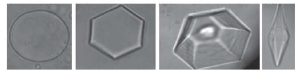
where is a double well potential with minima at and This is an Allen-Cahn energy in the curvature, different than an Allen-Cahn energy for a scalar embedded in the interface. Since has regions of concavity the surface diffusion is required to make the system well-posed. The mass of is conserved under (2.9), so a supporting line can be added to the well and there is no loss of generality in assuming that has equal depth wells. This is a simplistic model of interfaces formed by the freezing of water blended with antifreeze polymers that lower the freezing point. The polymers favor flat interfaces, or interfaces with large curvatures whose induced radius is smaller than the radius of gyration of the polymer, see Figure 2. That is, high interface curvatures exclude the antifreeze polymers. A penalty term that constrains the perimeter of the interface is added as a simple proxy for enclosed volume. This accounts for the relation between freezing temperature and polymer density within the enclosed liquid, driving the enclosed liquid volume to a value predetermined by available polymer. The combined energy takes the form
| (4.1) |
where denotes the length of the curve and is a reference length. The curve length can be written as
so that the perimeter energy can be written as
Using (3.45) it is straight-forward to incorporate the perimeter energy yielding
and the associated faceting gradient-flow normal velocity
| (4.2) |
4.1. Formal Equilibrium and Quasi-Steady Analysis
We provide a rough sketch of a construction of families of equilibrium and quasi-steady faceted states of the Faceting energy, emphasizing how fixed-domain tools can be brought to bear upon these geometric problems. The structure implied in the functional-arc length variation relation (3.40) impacts the critical point construction. Phase-plane methods allow the construction of families of equilibrium from the solutions of the -periodic system
| (4.3) |
where is a free parameter associated to the total curvature constraint. Periodic solutions can be constructed by reparameterizing to -constant arc length scaled so that the solution is -periodic. For small values of and this yields periodic -pulse solutions that take values near and the two minima of . Using as an integrating factor yields the relation
| (4.4) |
and the associated first integral of the system
for some The arc length variation satisfies
Evaluated at these special solutions the -gradient normal velocity reduces to
which for a fixed value of can be tuned to zero by adjusting either the equilibrium length or the coefficient To generate an admissible equilibrium it remains to satisfy the closure conditions (2.8)-(2.9). For this we outline a process. For a fixed value of the area condition (2.9) is a proxy for the sum of the interior angles in a regular -gon. This condition is easily met since the area integral increases as , but decreases with Adjusting the number of pulses one can make the net angle within of . The value of can be adjusted to yield an exact angle condition. The first closure relation ensures the curve terminates where it started. Exploiting periodicity, breaking the domain into equal pieces, traces out identical curves over each piece. Moreover, for the image of each piece approximates a corner of angle . Such shapes can generically be assembled in a fashion into a closed curve.
A more flexible construction yields quasi-stationary solutions by splicing together heteroclinic connections of the critical point equation on the line. Without loss of generality arc length is taken to be -constant. Let be the heteroclinic solution to (4.2) with on that connects to To satisfy the closure constraints (2.8)-(2.9) we fix and distance , modifying to given by
| (4.5) |
and is smooth and monotone for . So defined, is exponentially close, , to as for some We define the front quasi-equilibrium
where is a partition of into successive up and down heteroclinic orbits. Under the condition that the localized fronts do not overlap and has regions where it equals and where it equals zero. The function can be translated so that , verifying that it is -periodic. The closure constraints impose three restrictions on the shift locations, accounting for translational invariance leaves free parameters. Adjusting to balance the length eliminates the perimeter term and satisfies the first-integral equation up to exponentially small terms. That is, exactly, while the functional and arc length variations satisfy
where characterizes the exponentially small residuals.
 |
 |
 |
 |
 |
 |
 |
 |
 |
 |
In the limit we anticipate quasi-adiabatic dynamics in the front positions . We write and expand
where is a constant. The flow (3.51) takes the form
where the -scaled residual drives the slow dynamics of the front positions. The dominant linearity is given in (3.52). The exact linearization has corrections that arise from being a quasi-equilibrium. These can be incorporated into the residual terms. The nonlinear terms arising from the expansion about are formally lower order. This quasi-adiabatic framework has been successfully applied to rigorously capture the slow front dynamics when the parameters evolve on a slower time scale than that of the relaxation for [Promislow (2002)], [Doelman et al (2007)]. This approach requires a spectral dichotomy for the operator . The operators are taken to be piece-wise constant in time, subject to updates on time scales that are long compared to the relaxation time of the error term. Arc length can be taken to be spatially and temporally constant on the slow time scales, with spatial reparameterized at each temporal jump point setting the updated arc length to be constant over
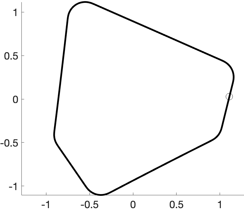
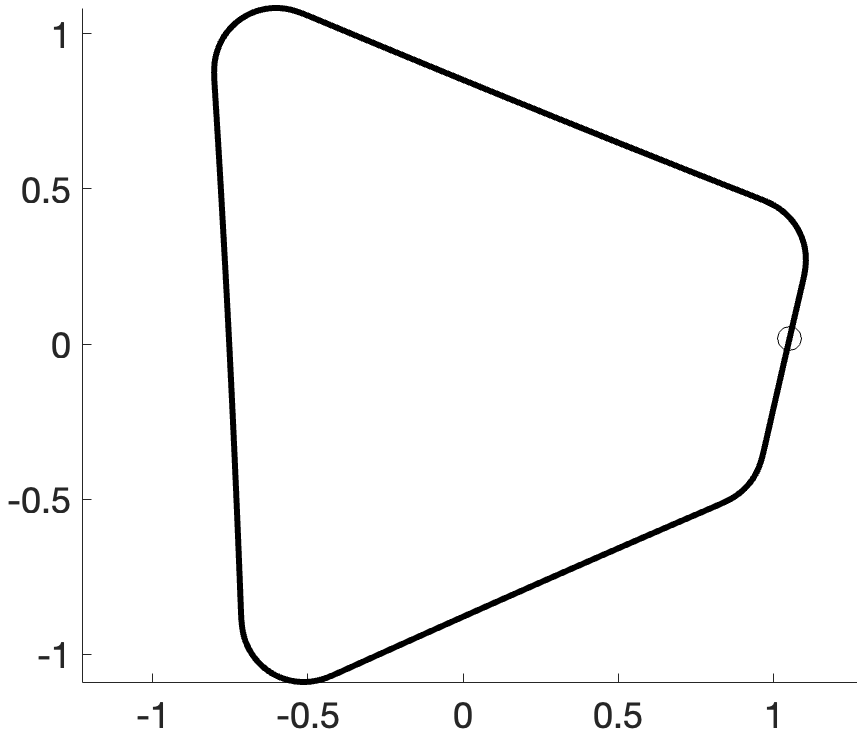
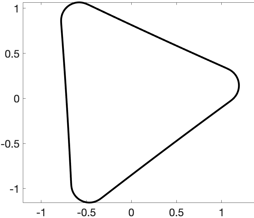
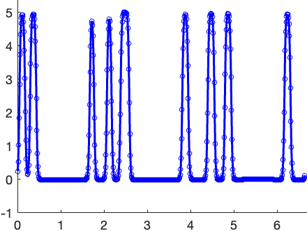
4.2. Computational Results
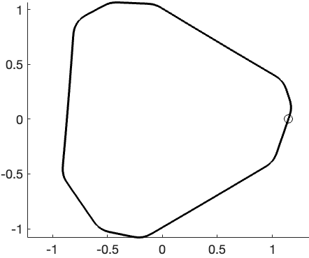
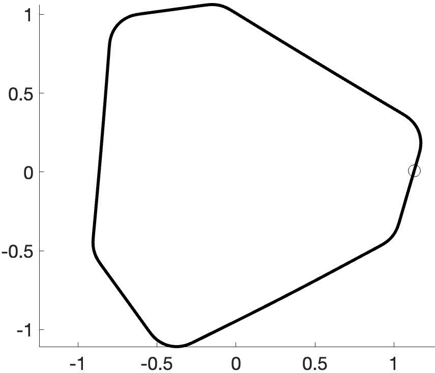
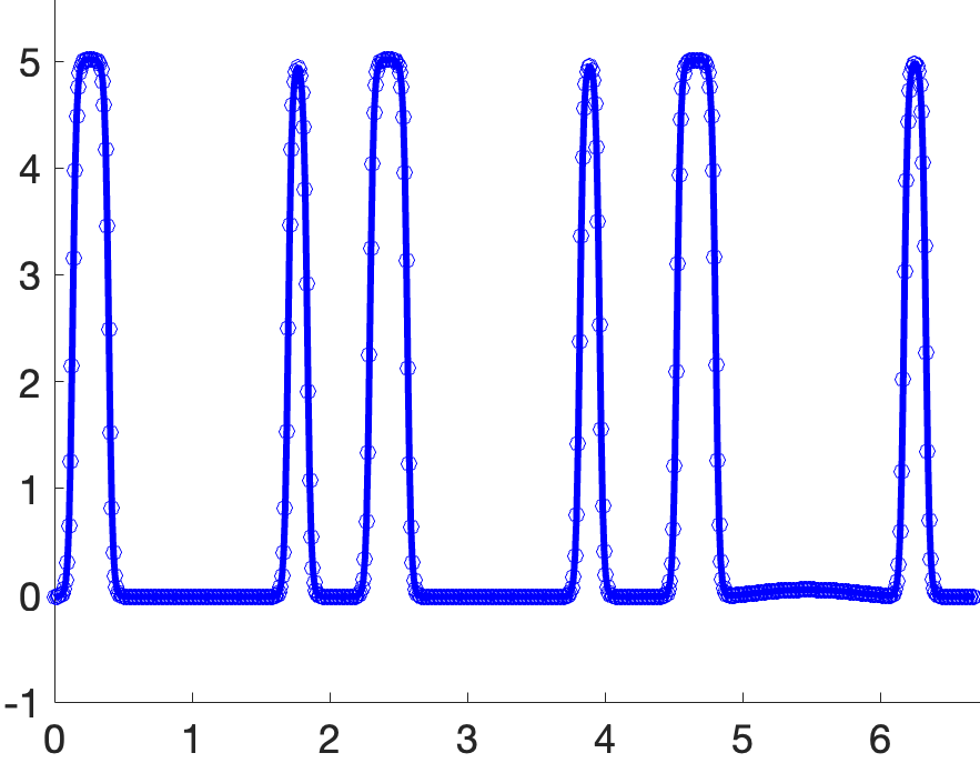
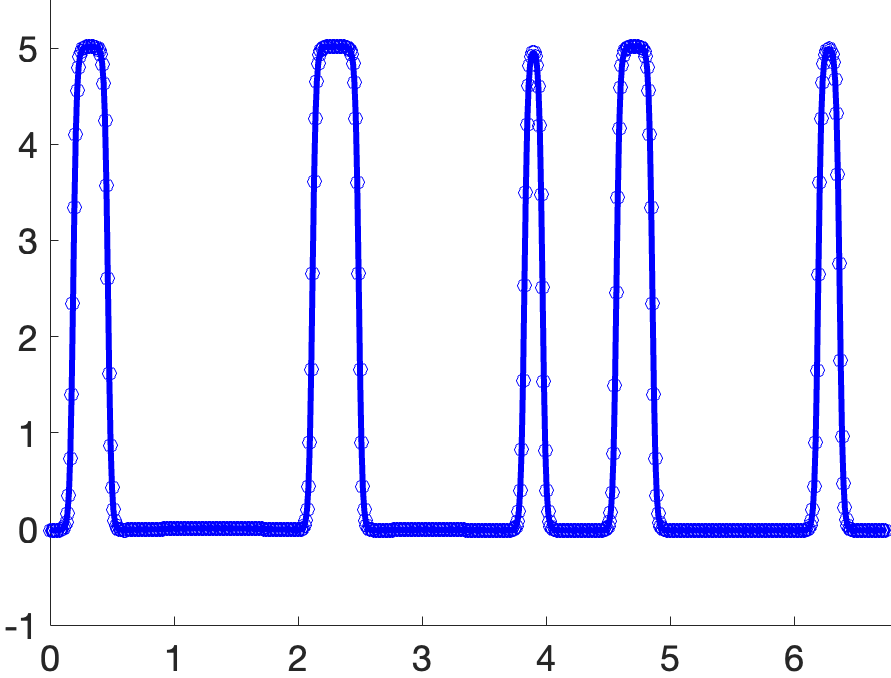
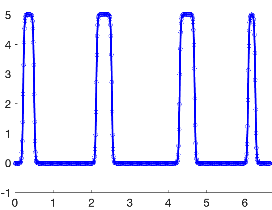
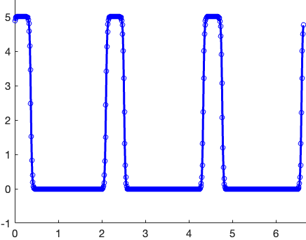
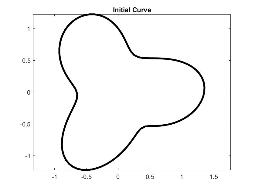
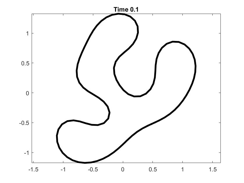
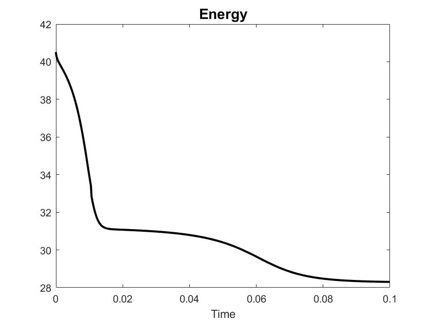
We supplement discussion of the quasi-adiabatic reduction with numerical simulations of the gradient flow (4.2) associated to the faceting energy. A description of the numerical scheme is presented Section 7.1 of the Appendix. Figure 3 gives the system parameters and the images of the interface and the associated curvature at sequence of five computational times as indicated. The initial spinodal decomposition yields 18 fronts that arrange into 9 pairs of up-down fronts that range from zero curvature to curvature near These coarsen in several events finally arriving at an equilibrium comprised of six fronts arranged symmetrically to yield an equilateral triangle with -rounded corners. Collectively this represents quasi-steady front motion converging to a symmetric equilibrium, illustrating the dynamics suggested by the approach sketched above. Figure 4 presents a semi-log plot of the system energy and functional variation residual versus time. The energy decays monotonically, with sharp stair-step drops at the coarsening events. The functional residual converges at to a value of , with six subsequent sharp excursions corresponding to the coarsening events that take the 9 pairs of fronts down to 3 pairs. The quasi-adiabatic analysis has the potential to capture the system evolution during the regimes
5. Two-Point Energies
In many applications interfaces have long range self-interactions. Generically these induce a long-range self-attraction and a short-range self-repulsion. Models of these are naturally described via a two-point self-interaction kernel that govern interactions between two points of the interface. For a rapidly decaying kernel the two-point interactions are dominated by contributions from near contact points: sections of interface that are well separated in arc length but proximal in physical space. Near contact points are not self-evident from the intrinsic coordinates of the curve. Two-point energies break the intrinsic coordinate formulation of the energy, incorporating a kernel based upon the spatial distance between two points on .
5.1. Bounded Two-Point Kernels
We introduce a two-point interaction kernel A and associated energy
| (5.1) |
where is the two-point distance vector and the subscript on the surface measure indicates the variable of integration. The two-point interaction kernel . Indeed we avoid potentials that are unbounded at partially due to numerical complications associated with infinite self-interaction energy of adjacent parts of the curve but also because self-intersection energies are indeed not infinite in physical reality.
To take variations of the energy it is convenient to parameterize the variations through the extrinsic vector field Using as a parameterization variable the path (3.2) induces a path, whose first variations satisfy
| (5.2) | ||||
The -formulation avoids the need to invert to write in terms of From these relations the variation of the adhesion energy takes the form
| (5.3) | ||||
Here acting on A denotes differentiation with respect to its single variable and all terms that are not first variations or extrinsic vector field are evaluated at The integrals over and are interchangeable up to , so the and terms can be combined with their unmarked siblings. This simplification and an integration by parts yields the reduced expression
| (5.4) | ||||
where the prefactor drops out since Introducing the two-point force
and the scalar surface energy density
the two-point energy extrinsic gradient satisfies
| (5.5) |
This motivates the definition
| (5.6) |
and the associated two-point -gradient normal velocity
| (5.7) |
The energy independence under rigid body motion implies that and resides in the range of . Surprisingly the rigid body energy independence leads to non-trivial relations, see Lemma 6 in Section 7.3 of the Appendix. This orthogonality allows us to define the associated intrinsic gradient through the inverse of
| (5.8) |
This leads to the two-point -gradient flow
| (5.9) |
At an equilibrium the linearization of the flow takes the form
which is a similarity transformation of the second extrinsic variation of the energy. Unlike the intrinsic 2nd variation, , the extrinsic 2nd variation is not generically self adjoint, and neither is Indeed it can also be expressed in the product formulation analogous to (3.51). The second variation of the two-point energy is complicated by the mixture of local and nonlocal operators and by the role of the . Simplifications can be obtained by scaling the two-point kernel to have an effective support that is small in comparison to the inverse of the norm of the curvatures of the curve. In this case the integrals over can be approximated by local contributions from near-intersection points. We pursue this scaling in the context of an adhesion-repulsion form of the two-point energy.
 |
 |
 |
 |
 |
 |
5.2. Application: Canham-Helfrich Adhesion-Repulsion Energy
A two-point adhesion repulsion energy arises from a bounded interaction kernel A with a Lenard-Jones type structure. More specifically A has a single, negative minima at a positive separation distance, a positive global maxima at zero, and tends to zero with growing separation distance. The interaction kernel drives the interface to pair disjoint sections of itself at an optimal separation distance while penalizing but not precluding self intersection. We investigate the properties of a two-point adhesion-repulsion kernel by pairing it with a weak Canham-Helfrich curvature term and a strong perimeter penalty,
| (5.10) |
Here denotes the image of the initial curve and the “precompression-factor” is the ratio of the initial curve length to the equilibrium curve length. For and this is a penalty term that models fixed densities common in biological membranes. The case corresponds to precompression induces a short transient interface lengthening and concomitant buckling motion that seeds bifurcations in subsequent long-term behavior. We take the adhesion-repulsion interaction kernel in the functional form
| (5.11) |
The potential takes is maximum value at , is negative for , has a single minima at with a negative value,
which is independent of . This Lennard-Jones type form enforces exponential decay of the interaction as is typical of electrostatic screening from a polar solvent.
The normal velocity takes the form
| (5.12) |
5.3. Formal Near-self-intersection Analysis
The short screening length regime is physically interesting for electrochemical settings. The rapid decay of interaction energy with distance simplifies the analysis. We present a heuristic characterization of the energy in a generic near self-interaction event. Assuming that absolute value of curvature is bounded by , then the arguments of a pair of close-approach points with must satisfy the “turning radius” condition . If further, the point is a local minimum of the distance function then we have and In the regime and the interaction kernel decays more quickly than the curvature can bend the curve, the interaction energy generated by a close-approach point is approximated to leading order by integrals over parallel lines a distance apart, both parameterized with constant arc length. The dominant contribution arises from . We fix , for on the same line as the contribution to since there. For the integral in over the opposite line we have
The distance while We have the expression
We assume and introduce the scaled distance The contribution from the opposing line yields
where we have introduced
Since the normal force imposes a stable equilibrium distance
between the near contact pairs. For the B term similar arguments show that the dominant contribution arises from the self-interactions of with the line containing . On this line the dominant contribution arises at
This term is lower order, scaling with , while converges to a non-zero limit for
Returning to the Canham-Helfrich Adhesion-Repulsion energy, for a curve with and curvature bounded in , the normal velocity at a near-approach point with satisfies
where is independent of and For sufficiently large value of and small value of the normal velocity will seek to stabilize the scaled optimal separation distance
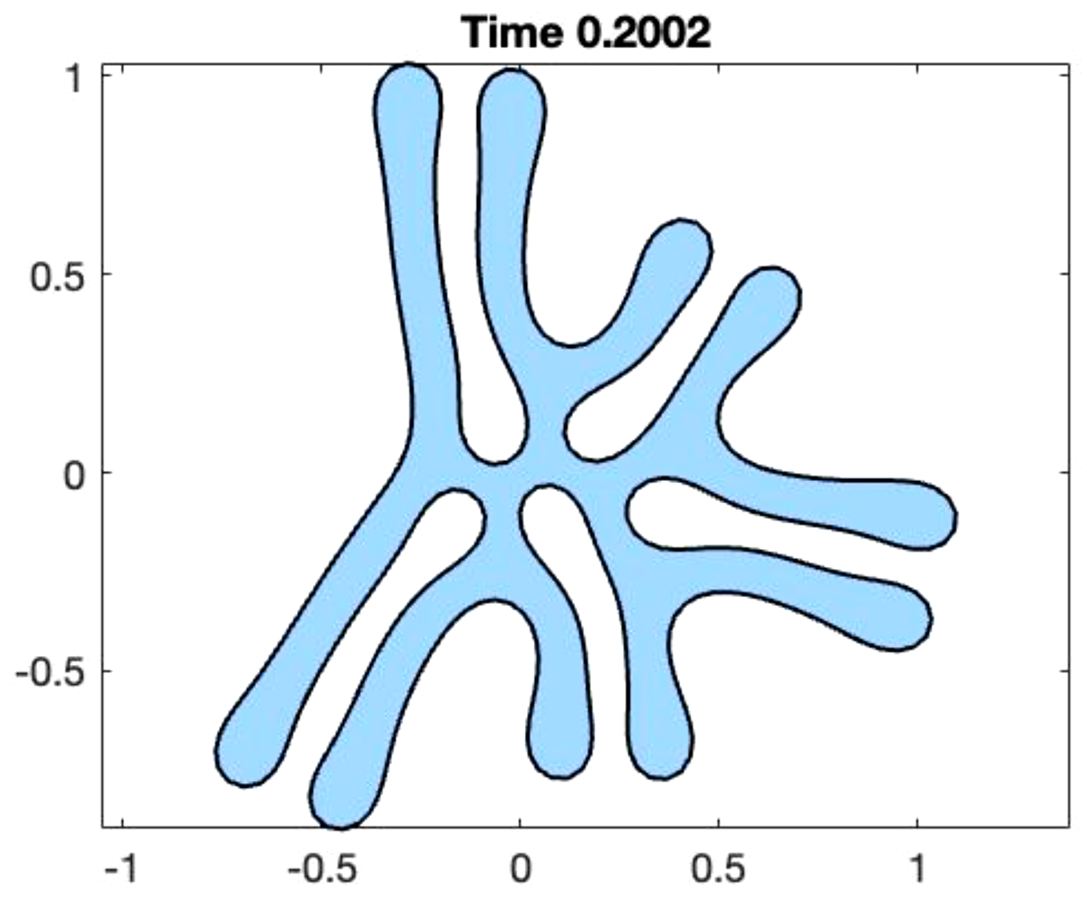
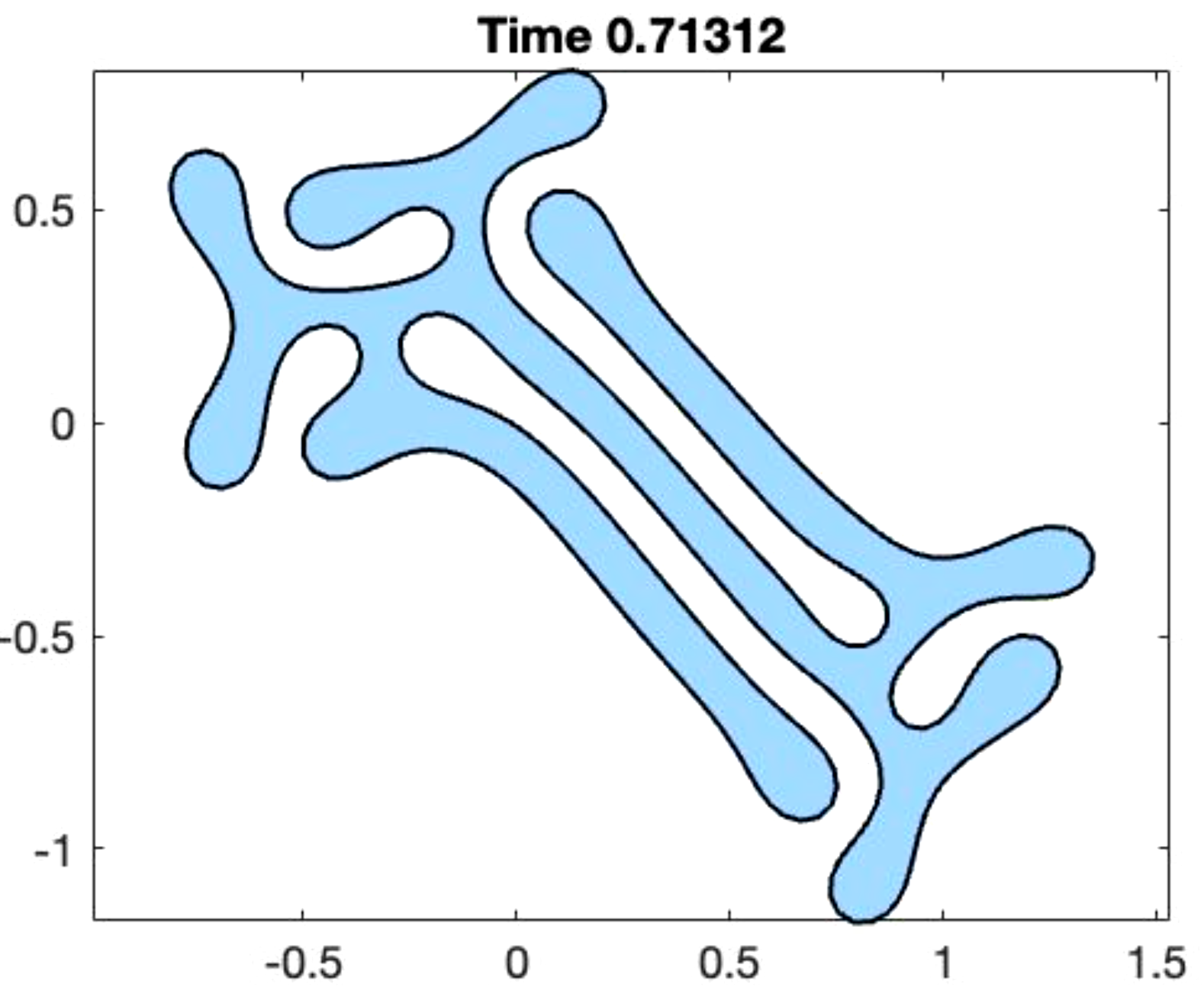
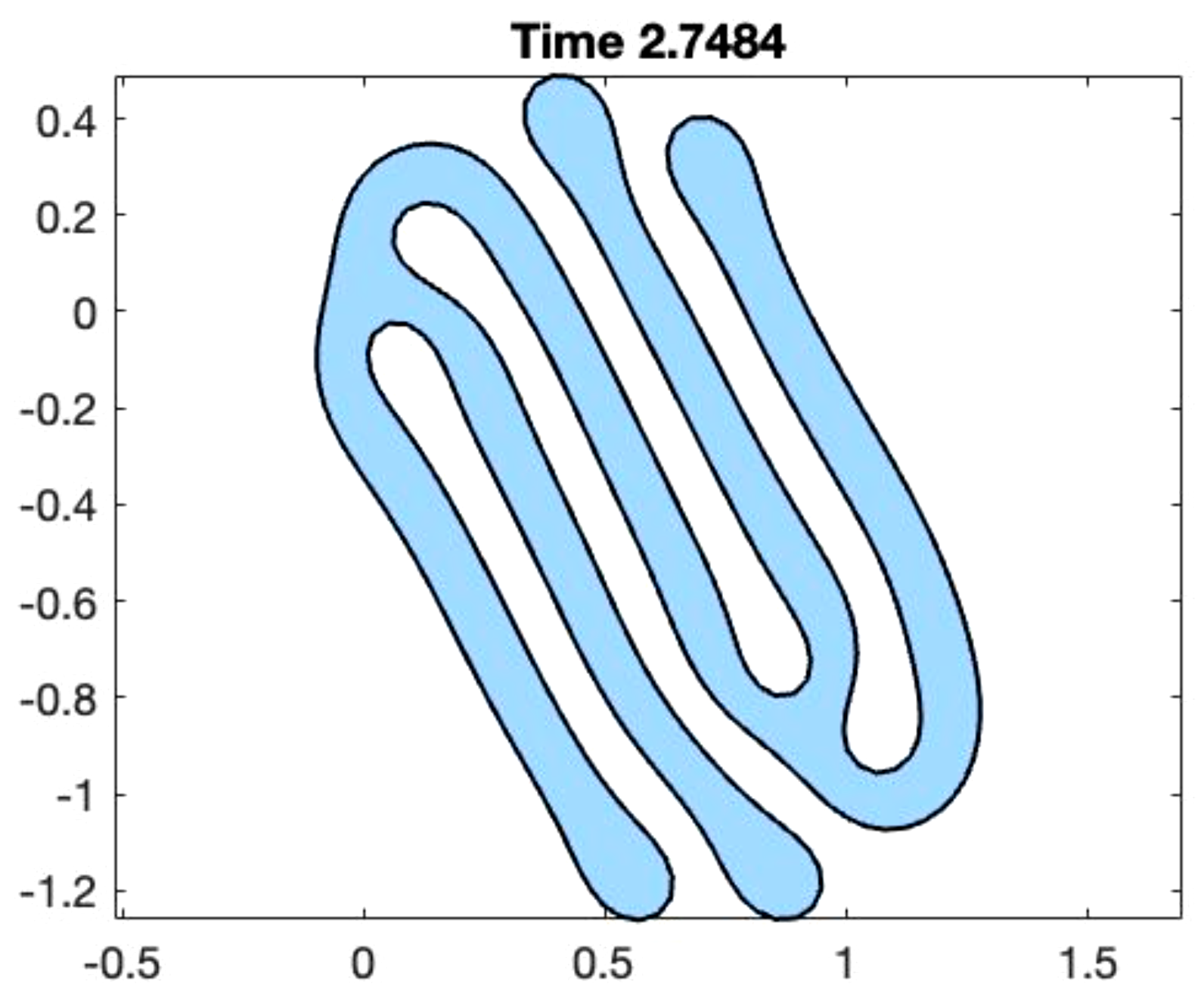
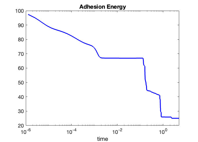
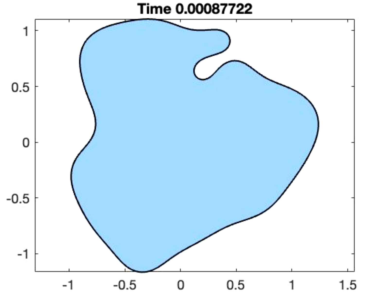
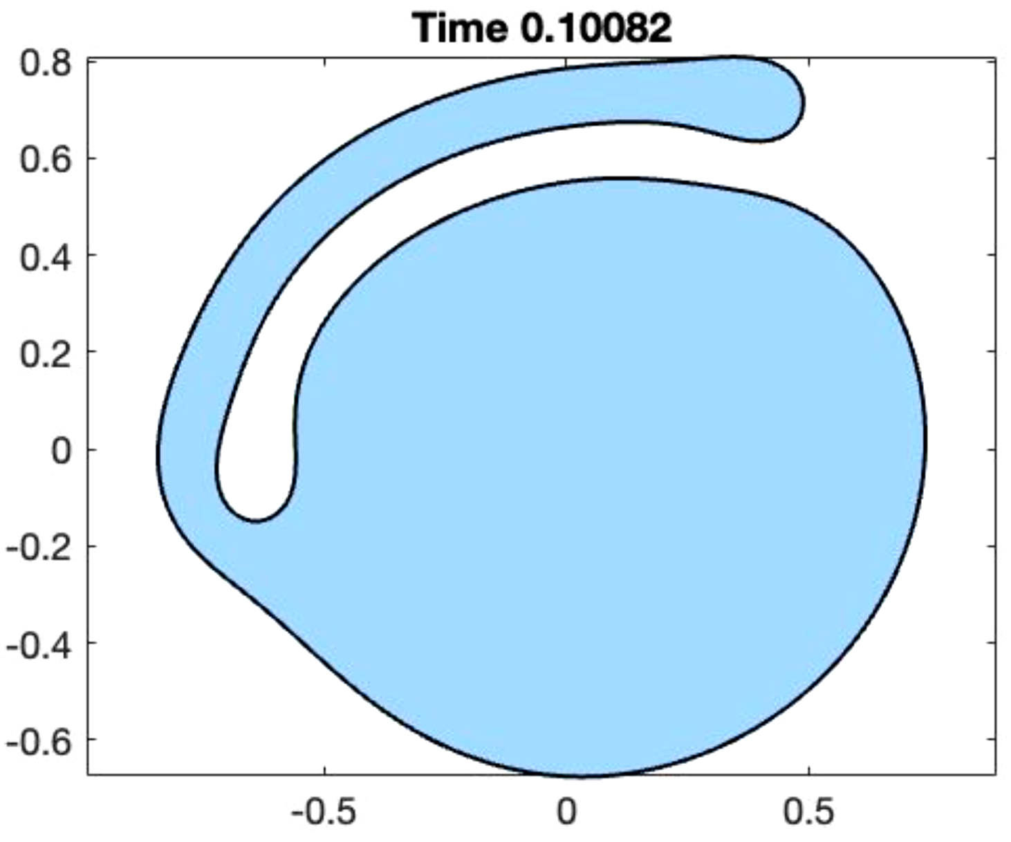
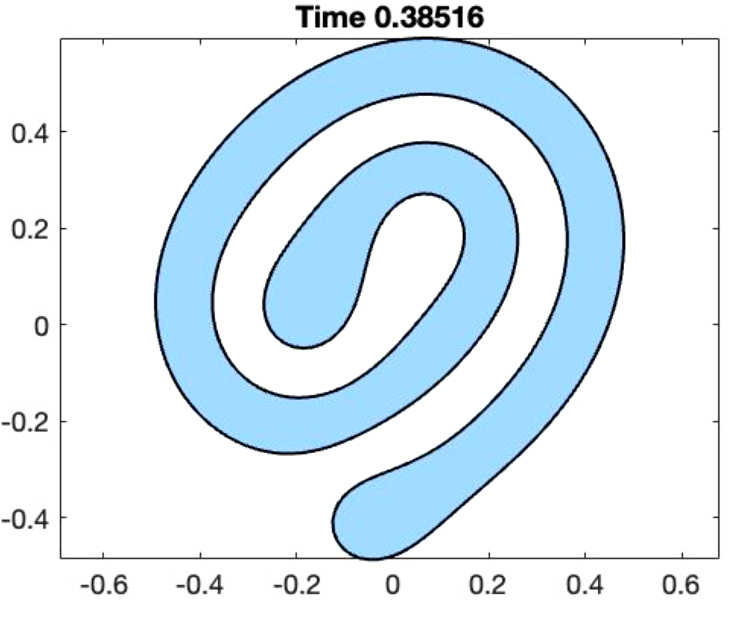
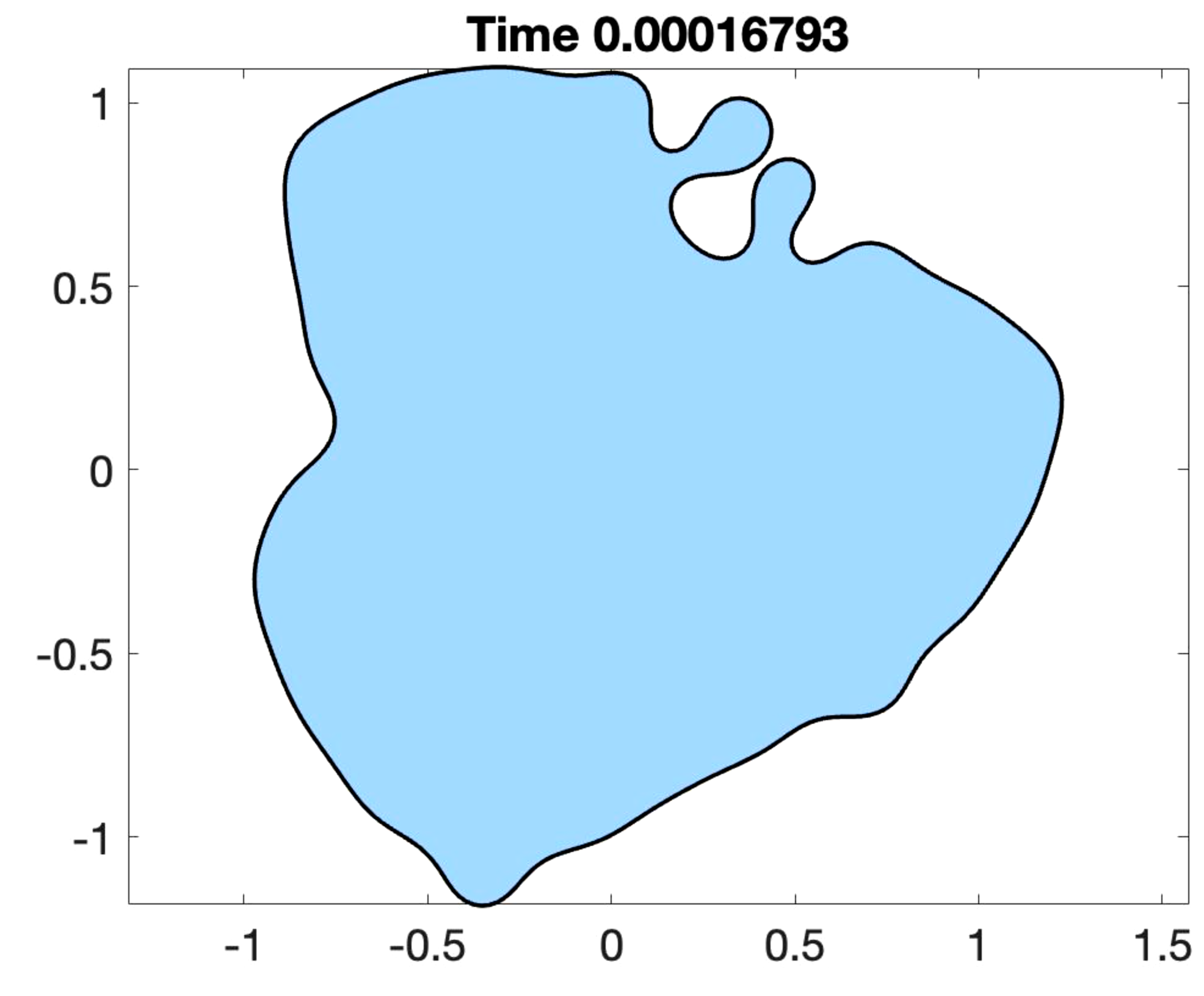
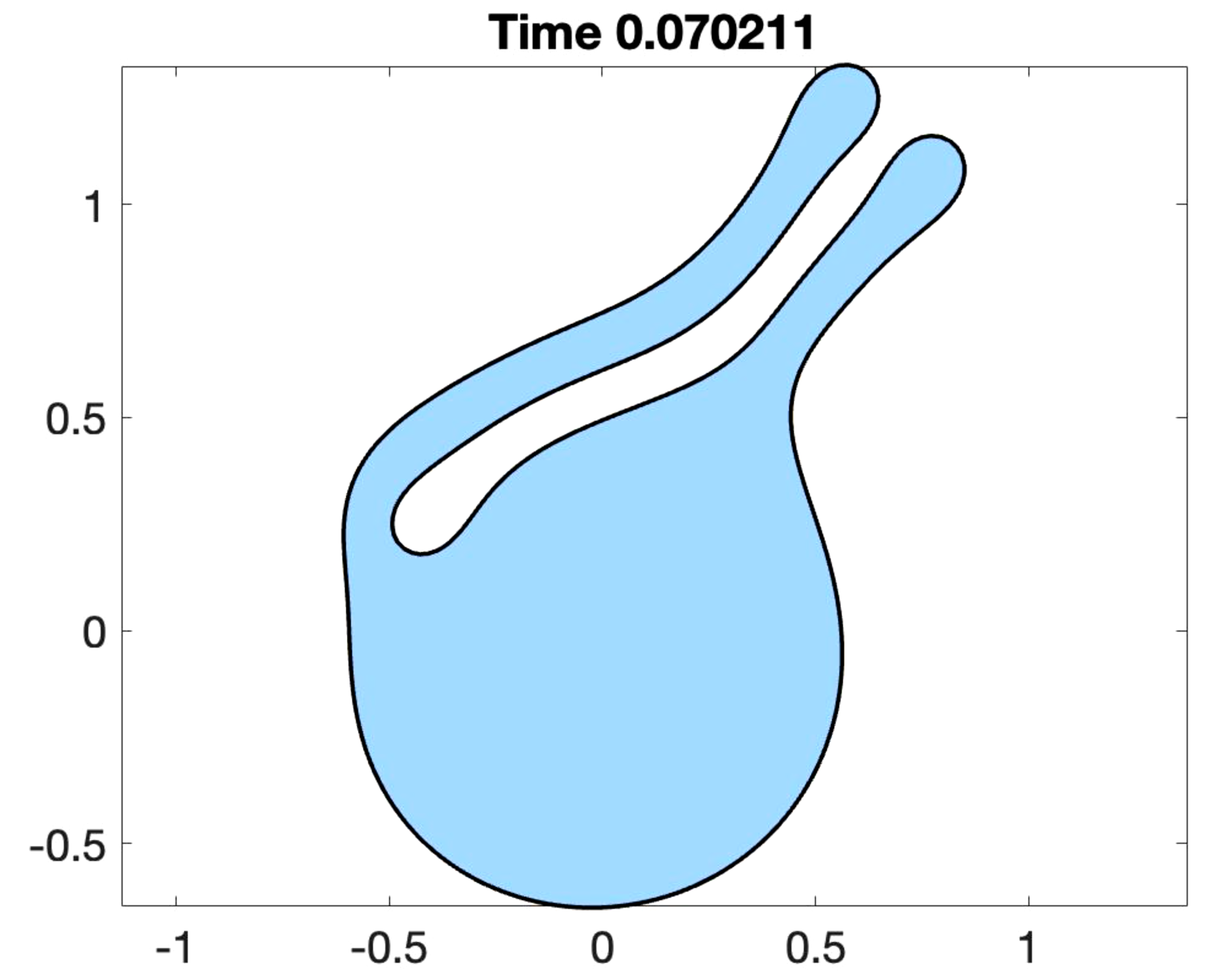
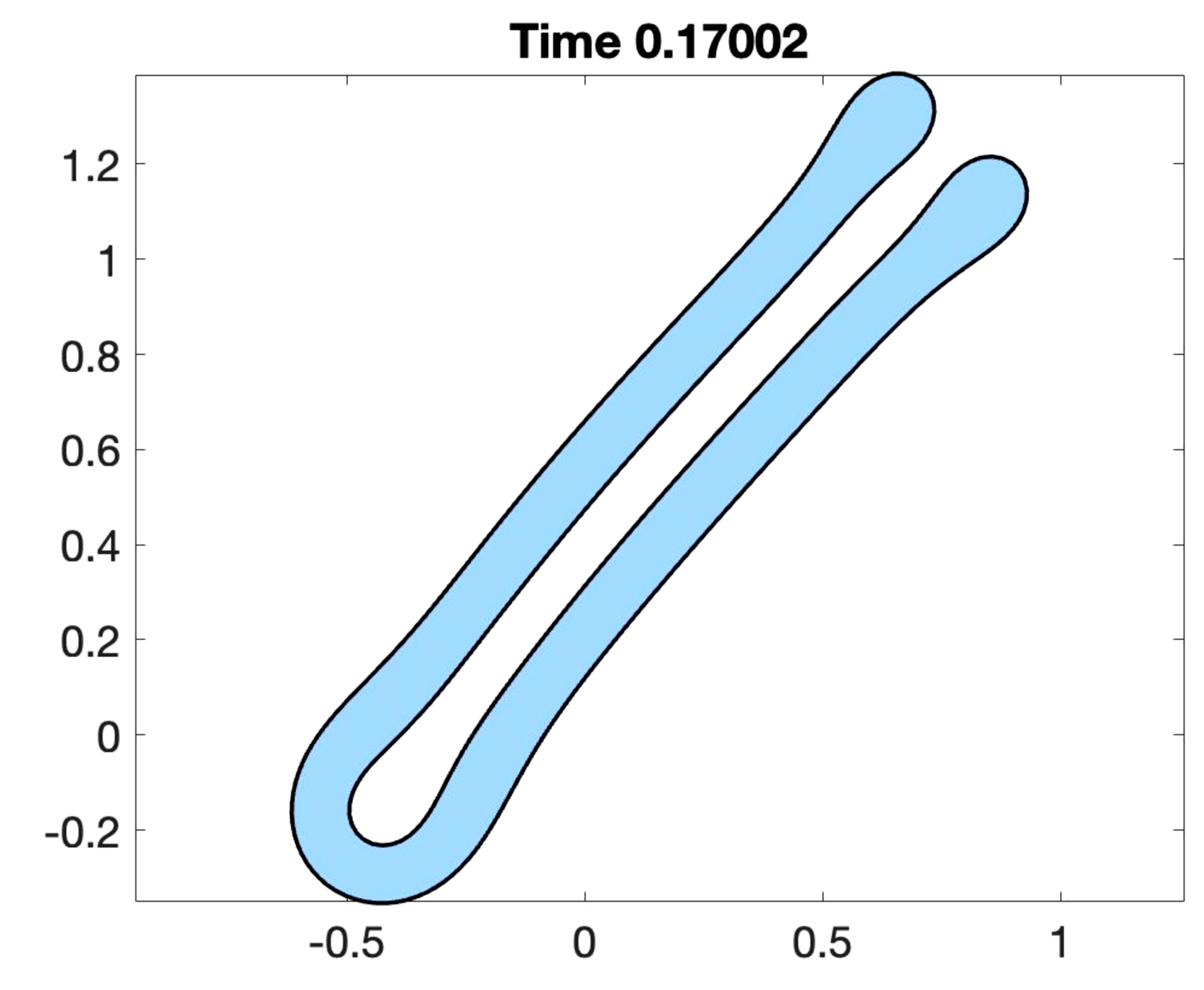
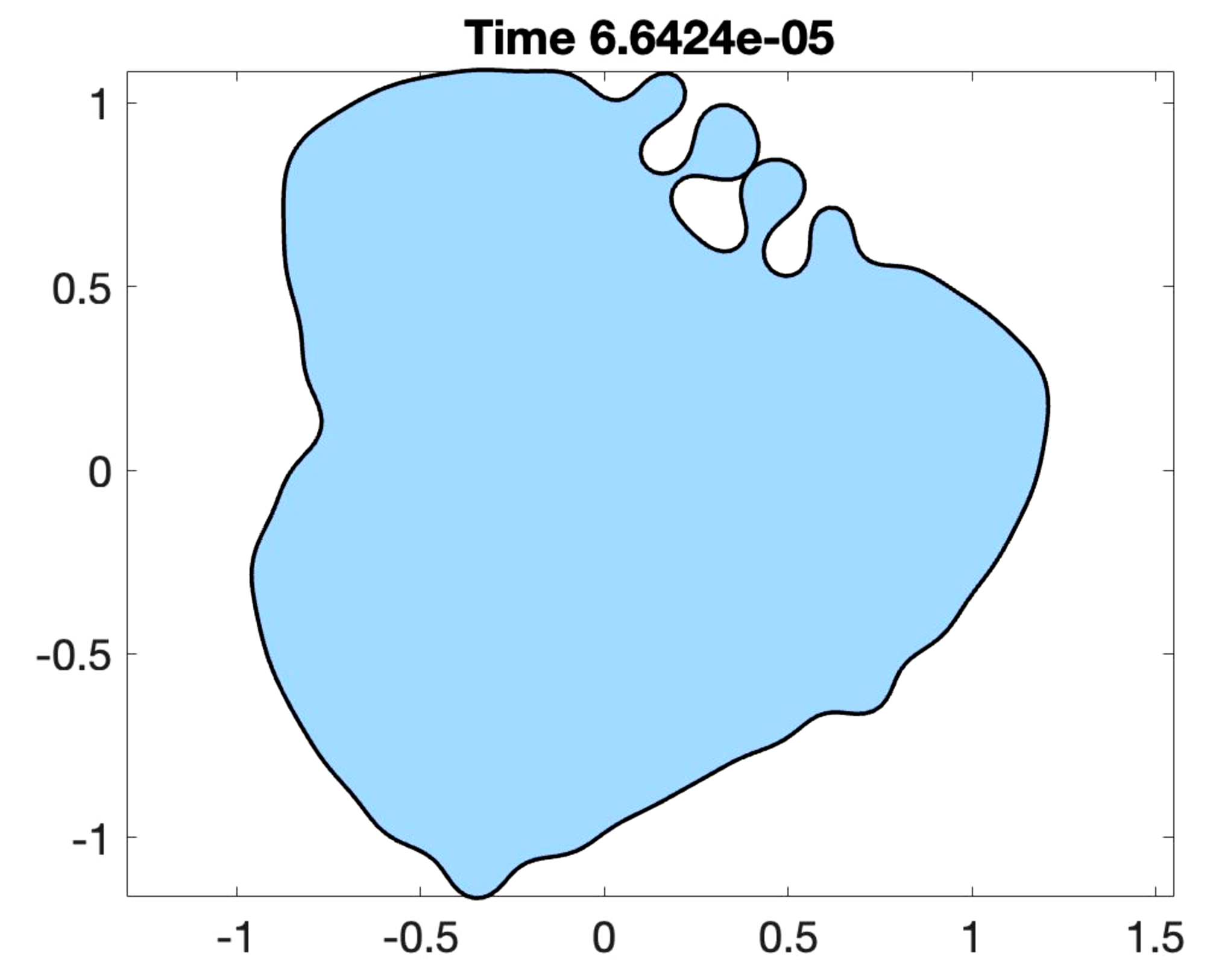
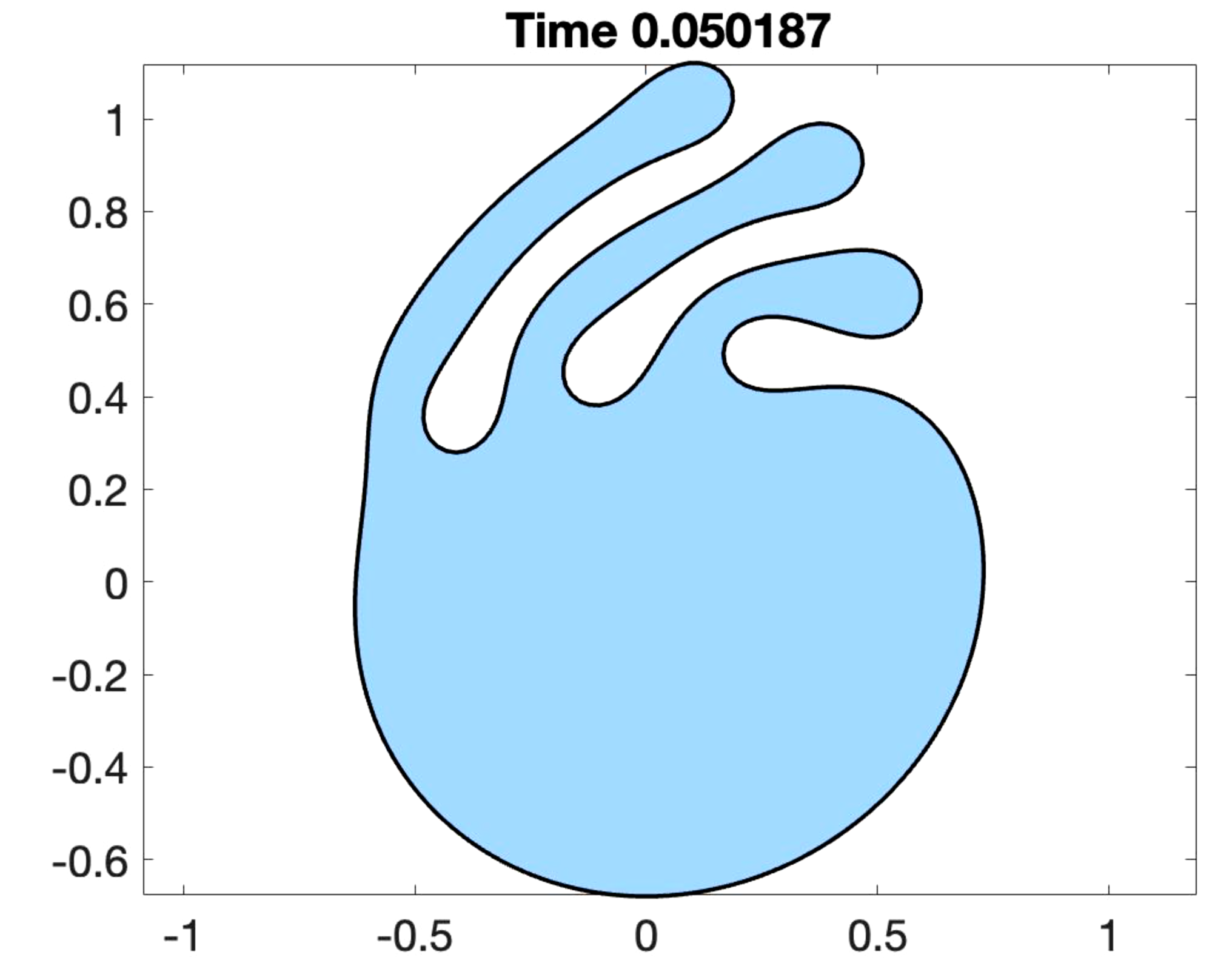
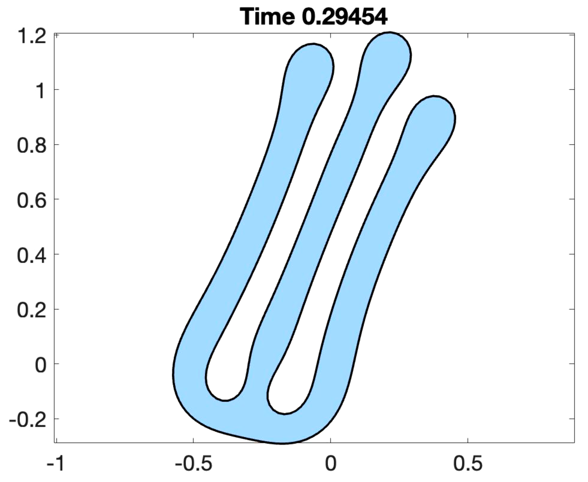
5.4. Simulation of Canham-Helfrich Adhesion-Repulsion Gradient Flow
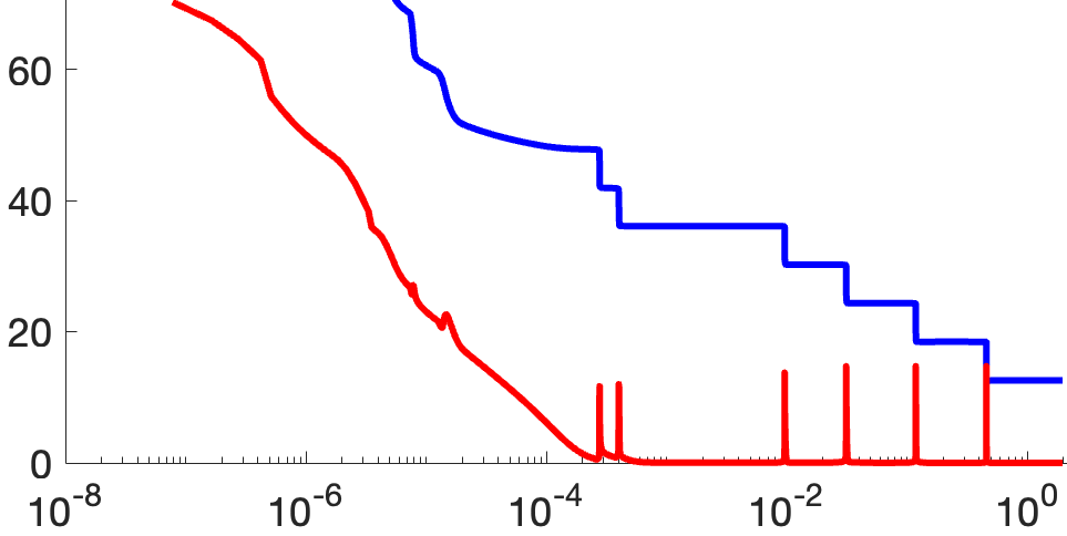
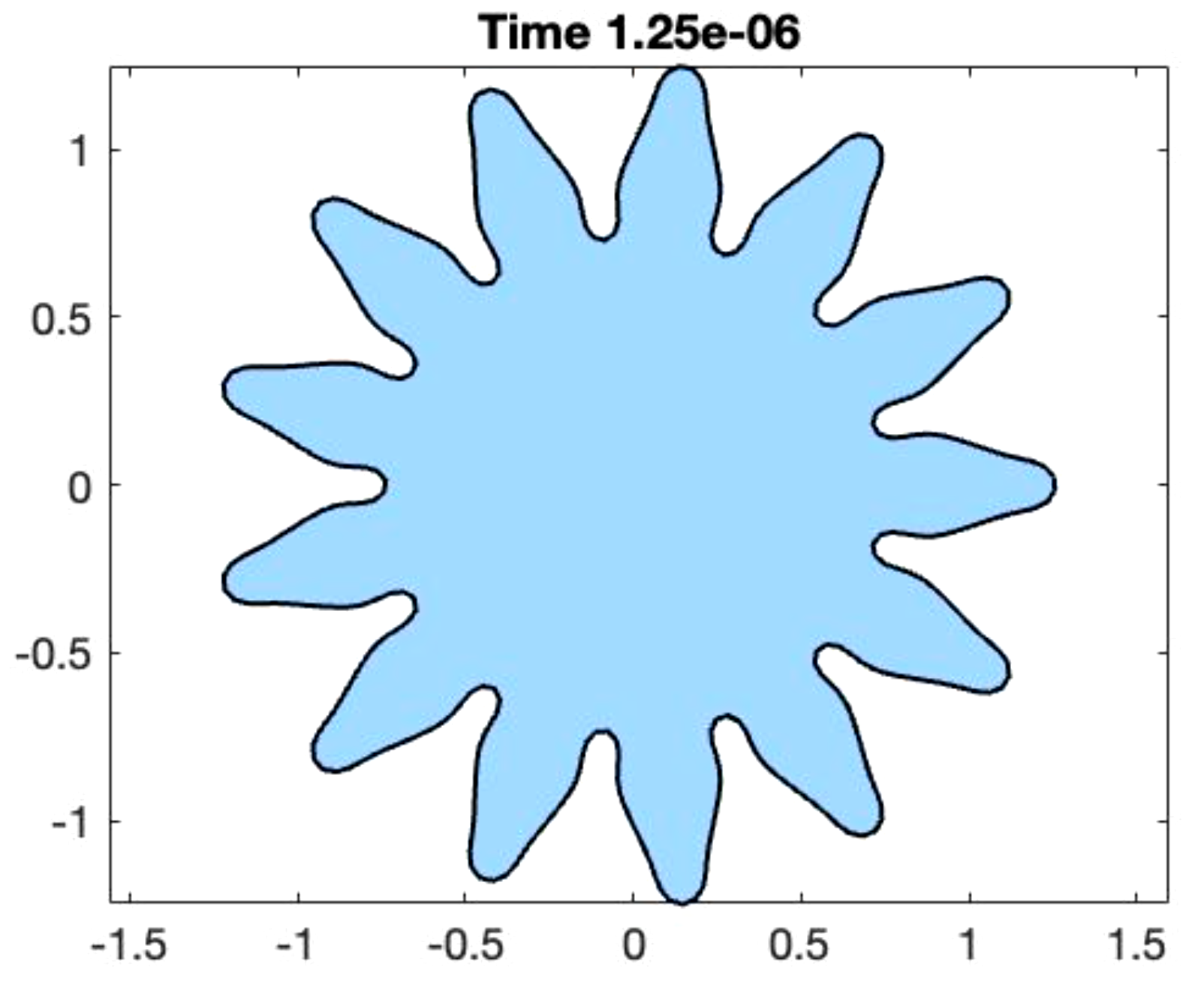
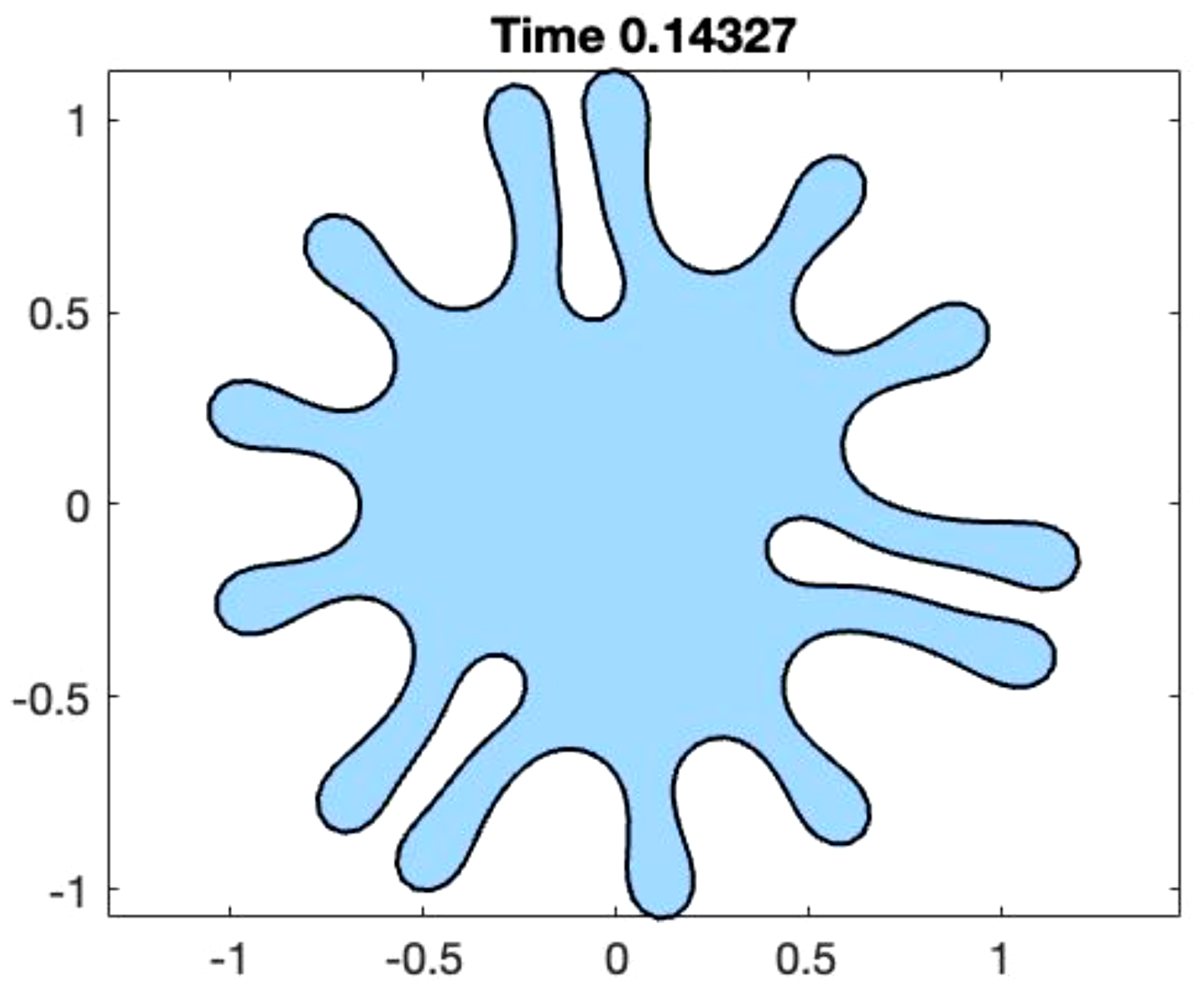
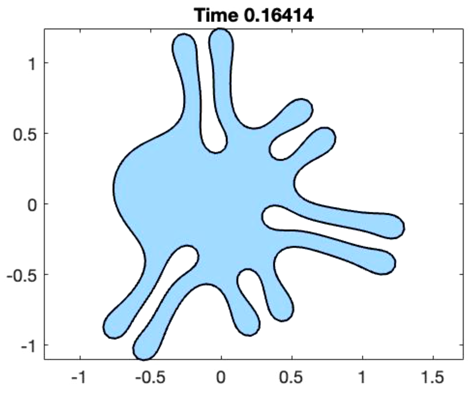
We supplement the formal arguments of the Section 5.2 with numerical simulations of the gradient flow. Figure 5 shows the time evolution of the Canham-Helfrich Adhesion-Repulsion gradient flow, (5.12) starting from a crenulated initial interface as depicted in the upper-left panel. Parameter values are given in Table 1. The simulation encounters four distinct regimes. In the first regime, the flow preserves the 13-fold symmetry of the initial data as the interface buckles to achieve its equilibrium length and energy decays at an exponential rate. In the second regime, symmetry is broken by finger pairing while energy is relatively constant. Interfaces typical of this regime are given by (top-middle, top-right) simulations at and In the third regime, the evolution is dominated by labyrinthine patterns depicted in images (middle-left, middle-center) at times and . On this time scale the interfaces rearrange through a sequence of tight packings that lead to increasingly lower energy foldings. The final regime, shows slow relaxation to a locally optimal packing. This equilibrium is a layered state evocative of the Thylakoid membranes shown in Figure 1. At equilibrium the interface recovers a -symmetry not present in intermediate states.
 |
 |
 |
 |
 |
 |
 |
 |
 |
The large values of drives the system on a fast time scale to arrive at a near equilibrium interface length. On these fast time scales the evolution is dominated by motion against curvature regularized by the Willmore flow, see [Chen and Promislow (2023)] for analysis of this motion in a related system. The buckling nature of motion against curvature generates folds within the interface. Figure 6 depicts simulations arising from identical initial data with different values of the precompression parameter Increasing generates more folds on the short time scale which has a significant impact on the final folded state. The three simulations are for precompression factors and in the top, middle, and bottom rows respectively. The initial folds evolve into fingers that initiate a traveling-wave motion. The normal velocity lengthens the fingers, pulling them into parallel sheets on an intermediate time scale depicted in the middle column. On a long time-scale the flow reaches its final folded state, depicted in the third column. Increasing increases the final surface area and the number of folds. The effect on the end state is a bifurcation from a single ’rolled-up’ sheet into a family of two- and three-stacked layers of flat sheets. Increasing beyond the value can lead to curve crossing in the fast transient. Curve crossing is inhibited but not excluded as the repulsive term, scaled by , is finite, and can be overwhelmed by motion against curvature during the buckling transient. Indeed the simulation shows a glancing self-intersection event in the short-time column.
6. Discussion
We presented a derivation of the gradient flows of local and two-point interfacial energies in a general framework. Throughout the analysis interfaces are assumed to be far from self-intersection. Self-intersection requires total negative curvature in excess of For the faceting energy, which seeks to minimize negative curvatures this assumption generically holds for quasi-equilibrium states. Energies dominated by an adhesion-repulsion two-point energy generically do introduce negative curvatures, but the repulsion core inhibits self-intersection. Rigorous non-self-intersection results for these systems are plausible given uniform bounds on curvatures. For many of the energies proposed it is straightforward to demonstrate the existence of global minimizers over function spaces on that incorporate spatially constant arc-length parameterization, the challenge is to show that any minimizer so constructed does not non-self intersection.
A foci for future work is to conduct the spectral analysis of linearization about stationary and quasi-steady patterns. The spectral analysis of spiral waves which arise as reductions of reaction-diffusion systems is well established [Sandstede and Scheel (2023)]. Bifurcations of classes of Delaunay surfaces immersed in have been conducted as an eigenvalue problem associated to energies whose critical points subject to enclosed volume or surface area constraints have constant mean curvature, [Koiso et al (2015)]. Both of these classes of results are encouraging.
The ultimate goal is to extend the analysis to study quasi-steady patterns and bifurcation in reaction diffusion systems on an evolving interface. Many problems of interest to biological membrane evolution can be formulated in terms of an energy coupling interfacial configuration to surface diffusion and reaction of active materials that are bound to the membrane, [Shemesh et al (2014), Aland et al (2014), Gera and Salac (2018)]. The recent development of computational tools for the bifurcations arising in these geometric problems should greatly increase the interest in this rich class of problems, further inspiring model development, [Meinder and Uecker (Arxiv)].
7. Appendix
This provides discussion of the numerical scheme and results that are tangential to the main issues.
7.1. Discussion of Numerical Scheme
We outline the approach to the numerical resolution of the normal velocity and present a numerical convergence study for an example problem. The approach employs the scaled arc length formulation over with The parameterization satisfies
| (7.1) |
for all where is the length of the curve. This has been used successfully in several previous works of the authors for a range of applications [Moyles and Wetton (2015), Pan and Wetton (2008)]. This choice of arc length results in simple expressions for spatial derivatives, in particular
| (7.2) | |||||
| (7.3) |
where denotes rotation by
For a convergence study we consider the Canham-Helfrich adhesion energy (5.10). We formulate the numerical approximation as a Differential Algebraic Equation (DAE) [Ascher and Petzhold (1998)] in which at each time step the vector positions , curvatures , higher derivatives , and normal velocities are approximated on an point stencil. The curve length represents one additional unknown. This yields an implicit system for the total unknowns through a second order finite difference in space in conjunction with implicit Euler time stepping. The equations are summarized below, with capital letters for the discrete variables with subscripts for spatial grid point and superscripts for time step.
- N equations:
-
With time step we have normal motion
where and is the periodic second order finite difference approximation of first derivatives
with and taken mod and .
- N equations:
-
We preserve scaled arc length at the next time step
(7.4) - N equations:
-
Relate the curvature to positions, this is a second order finite difference approximation of (7.2).
- N equations:
-
Relate the Laplacian of curvature to curvature, this is a second order finite difference approximation of (7.3).
- N equations:
- 1 equation:
-
There is an arbitrary constant in the tangential motion that needs to be fixed. This is accomplished by enforcing zero average tangential velocity:
The resulting nonlinear system for the unknowns at time level is solved using Newton’s method with hand coded Jacobian entries. Adaptive time stepping with a user-specified local error tolerance is used, with the local error for two steps with time step estimated by comparing to a computation with time step .
The discretized systems are highly nonlinear and stiff, sixth order in spatial variables for the adhesion energy models and eighth order for the faceting models. The high stiffness coupled with the DAE nature naturally suggest implicit time stepping methods. The dynamics feature a wide range of time scales which makes adaptive time stepping necessary. Accurately assessing the local error led to our use of Newton iterations for the implicit time steps. For the Newton iterations to be sparse solves, we used finite difference rather than spectral spatial approximation. Backward Euler was the simplest time stepping method to use, with the advantages of its good stability properties for stiff systems and the ease in which adaptive time stepping can be implemented. The extension of the system to include curvature, the normal velocity and other variables made hand coding the Jacobian matrix for Newton iterations practical. While level set methods [Osher and Fedkiw (2003)] can accommodate topological changes and easily extend to surfaces in 3D it would be a challenge to formulate the energetic effects considered in the models presented here.
For the convergence problem we take initial data
with . This initial parametrization is not scaled arc length, and a pre-processing step is conducted with Newton iterations to convert to scaled arc length in the approximate sense (7.4). The code includes a local smoothing strategy if these iterations do not converge, although that is not needed for this example. We take parameters in (5.10): , , and adhesion energy parameters , , . A run with grid points and local error tolerance is shown in Figure 7.
Keeping the local error tolerance fixed, we compute solutions with , 100, 200, 400, and 800 spatial grid points. We compare the maximum norm difference in position variables at common grid points between successively refined solutions in Table 2.
| ratio | ||
|---|---|---|
| 50 | 0.1909 | |
| 100 | 0.0397 | 4.8 |
| 200 | 0.0101 | 3.9 |
| 400 | 0.0024 | 4.2 |
The error decreases by approximately a factor of 4 at each doubling of grid points, confirming second order spatial convergence.
We also confirm the behavior of the adaptive time stepping by local error tolerance , , , with fixed. The computation takes 65, 180, 571, and 1811 total time steps, respectively. With each ten-fold decrease in error tolerance the number of time steps taken increases approximately by a factor of . This is consistent with a correctly identified second order local temporal error.
The MATLAB code that generated the results for the convergence study is available [Wetton (2024)]
7.2. Reparameterization and Tangential Flow
It well known that reparameterization has a direct connection to tangential motion of an interface, [Mantegazza (2011)]. For completeness we include a derivation. We consider a one-parameter family of mappings with expansion
| (7.5) |
where The reparameterization induces the interface map This reparameterization induces an extrinsic vector field characterized in the follow lemma.
Lemma 4.
Given a curve with curvature and arc length pair . The first variation of induced by the one-parameter family of reparameterization maps in (7.5) induces intrinsic perturbations that correspond to the purely tangential extrinsic vector field
Proof.
The perturbed interface map admits the expansion
Acting with yields
The perturbed arc length has the expansion
which we write as
| (7.6) |
From this we deduce the expansion
The tangent vector expands according to
Distributing the derivative and using (2.3) to replace the surface gradient of the tangent yields
| (7.7) |
We use (2.2) to expand the curvature,
where we chose the sign that aligns with We rewrite the curvature perturbation as
| (7.8) |
Combining (7.6) and (7.8), the domain variation under the mapping induces the perturbations
| (7.9) |
∎
Proof.
It is sufficient to act out the operator on the arc length variation term in (3.35) and observe that it cancels with functional variation term. We consider in cases by the type of variable dependence. In all cases the factors of cancel in arc length variation. For ,
For the case the identify reduces to
Finally for the case the identity is an immediate application of the chain-rule. ∎
7.3. Two-Point Curve Invariants.
We establish the following invariants associated to the two-point interaction kernel acting on smooth, closed, non-self-intersecting curves.
Lemma 6.
Let be a smooth map whose image is closed and non-self-intersecting. Define the distance vector via The product space admits the decomposition
in terms of the -level sets
Let denote the arc length of the parameterization of and denote the one-dimensional Hausdorff measure on Then satisfies the equalities
| (7.10) | ||||
| (7.11) |
for each and each Here denote the normal and tangent to at while a tilde superscript denotes evaluation at .
Proof.
Lemma 2 establishes that the kernel of is comprised of the infinitesimal generators of the rigid body motions of . We first consider the rotational invariant. Using the formula (5.6) and the representation of the rigid body rotation the invariance of energy under rigid rotation implies that
where we used (2.3) to rewrite Since integrating by parts on the second term yields
On the other hand so that
| (7.12) | ||||
We apply the co-area formula to rewrite the integral over to one over the level sets of . Specifically we rewrite the last integral in terms of , so that
The gradient of satisfies
where a tilde denotes evaluation at Since the co-area formula allows us to rewrite the last integral in (7.12) as
Within this derivation the two-point interaction kernel is an arbitrary smooth function. The integral over is in and is zero at where Since can take dense values in the result (7.10) follows.
Rigid translates are induced by the extrinsic vector field where is an arbitrary constant vector. We deduce that
Following the same steps yields (7.11). ∎
Remark 2.
The sets are each comprised of a finite collection of disjoint components of Under the assumption that does not self-intersect, comprises the diagonal of the product space and for small enough comprises two disjoint curves that are symmetric about the diagonal. More generally, from the implicit function theorem, for each non-degenerate level set, defined below, there are a finite collection of functions such that that satisfy the relation
subject to initial data from distinct connected components of The equation for is well defined so long as This quantity is zero when the circle of radius about intersects the image tangentially, indicating a boundary point of a component of the level set Non-degeneracy means that zeros of are transverse in for fixed
Acknowledgment
The second author recognizes support from the NSF through grant NSF-2205553. The third author recognizes support from NSERC Canada. The authors anticipate development of a freeware code library for general interfacial gradient flows described in this paper.
References
- [Aland et al (2014)] S. Aland, S. Egerer, J. Lowengrub, A. Voigt, Diffuse interface models of locally inextensible vesicles in a viscous fluid, J. Comput. Physics, 277 (2014), 32-47.
- [Alikakos and Fusco (2008)] N. Alikakos and G. Fusco, On the connection problem for potentials with several global minima, Indiana University Mathematics Journal, 57 (4) (2008), 1871-1906.
- [Alikakos et al (2006)] N. Alikakos, S. Betelu, and X. Chen, Explicit stationary solutions in multiple well dynamics and non-uniqueness of interfacial energy densities, Euro. Jnl. of Applied Mathematics, 17 (2006) 525-556.
- [Ascher and Petzhold (1998)] U. Ascher and L. Petzhold, Computer Methods for Ordinary Differential Equations and Differential-Algebraic Equations, Society for Industrial and Applied Mathematics, Philadelphia (USA), ISBN 978-0898714128.
- [Austin and Staehelin (2011)] J. Austin and A. Staehelin, Three dimensional architecture of Grana and Stroma Thylakoids of higher plants as determined by electron tomography, Plant Physiology 155 (2011) 1601-1611.
- [M’barek et al (2017)] K. M’Barek, D. Ajjaji, A. Chorlay, S. Vanni, L. Foret, A. Thaim, ER membrane phospholipids and surface tension control cellular lipid droplet formation, Developmental Cell 41 (2017) 519-604.
- [Barrett et al (2020)] J. Barrett, H. Garcke, R. Nürnberg. “Parameteric finite element approximations of curvature-driven interface evolutions”. In: Geometric Partial Differential Equations – Part I. Ed. by Andrea Bonito and Ricardo H. Nochetto, Vol.21. Handbook of Numerical Analysis. Elsevier, 2020. Chap. 4, pp 275-423, DOI 10.1016/bs.hna.2019.05.002.
- [Blanazs et al. (2009)] A. Blanazs, S.P. Armes, and A. J. Ryan, Self-assembled block copolymer aggregates: from micelles to vesicles and their biological applications, Macromolecular rapid communications, 30 (2009) 267–277.
- [Canham (1970)] P. Canham, Minimum energy of bending as a possible explanation of biconcave shape of human red blood cell, J. Theoret. Biol. 26 (1970) 61–81.
- [Helfrich (1973)] W. Helfrich, Elastic properties of lipid bilayers – theory and possible experiments, Z. Nat. Forsch. C 28 (1973) 693-703.
- [Chen 2007] Xinfu Chen, Spectrum for the Allen-Cahn, Cahn-Hilliard, and phase field equations for generic interfaces, Communications in Partial Differential Equations, 19 (7) (1994), 1371-1395.
- [Chen et al (2020)] Y. Chen, A. Doelman, K. Promislow, F. Veerman, Robust stability of multicomponent membranes: the role of glycolipids, Archives Rational Mechanics and Analysis 238 (3) (2020), 1521-1557 .
- [Chen and Promislow (2023)] Y. Chen and K. Promislow, Curve Lengthening via regularized motion against curvature from the strong FCH gradient flow, J. Dynamics and Differential Eqns., 25 (2023) 1785-1841.
- [Doelman et al (2007)] A. Doelman, T. Kaper, and K. Promislow, Nonlinear asymptotic stability of the semi-strong pulse dynamics in a regularized Gierer-Meinhardt model, SIAM J. Math. Analysis, 38 (2007) 1760-1787.
- [Gau et al (2006)] H. Gau, T. Sage, and K. Osteryoung, FZL, an FZO-like protein in plants, is a determinant of thylakoid and chloroplast morphology, Proc. National Academy Sciences, 103 (2006).
- [Gera and Salac (2018)] P. Gera and D. Salac,Modeling of multicomponent three-dimensional vesicles, Computers and Fluids 172 (2018) 362-383.
- [Giaquinta and Hildebrandt (1996)] Calculus of Variations. I, Grundlehren der Mathematischen Wissenschaften [Fundamental Principles of Mathematical Sciences], vol 310, Springer-Verlag, Berling 1996, ISBN 3-540-59625-X.
- [Gibson (2010)] M. Gibson, Slowing the growth of ice with synthetic macromolecules: beyond antifreeze(glyco) proteins, Polymer Chemistry 1 (2010) 1129-1340.
- [Koiso et al (2015)] M. Koiso, N. Palmer, and P. Piccione, Bifurcation and symmetry breaking of nodoids with fixed boundary, Adv. Calc. Var. 8 (4) (2015) 337-370.
- [Mantegazza (2011)] C. Mantegazza, Lecture Notes on Mean Curvature Flow, Progress in Mathematics, 290, Birkhäuser/Springer Basel AG, Basel (2011)
- [Meinder and Uecker (Arxiv)] A. Meinder and J. Uecker, Differential Geometric Bifurcatoin problems in pde2path – algorithms and tutorial examples, ArXiv:2309.03546v1 (2023).
- [Moyles and Wetton (2015)] I. Moyles and B. Wetton, A numerical framework for singular limits of a class of reaction diffusion problems, Journal of Computational Physics 300 (2015) 308-326.
- [Osher and Fedkiw (2003)] S. Osher and R. Fedkiw, Level Set Methods and Dynamic Implicit Surfaces, Springer, New York (USA), https://doi.org/10.1007/b98879.
- [Pan and Wetton (2008)] Z. Pan and B. Wetton, A numerical method for coupled surface and grain boundary motion, European Journal of Applied Mathematics 19 (2008) 311-327.
- [Pismen (2006)] L. M. Pismen, Patterns and interfaces in dissipative dynamics, Springer Series in Synergetics, Springer Complexity, (2006)
- [Promislow (2002)] K. Promislow, A renormalization method for modulational stability of quasi-steady patterns in dispersive systems, SIAM J. Math. Analysis, 33 (2002), 1455-1482.
- [Rupp (2024)] F. Rupp, The Willmore flow with prescribed isoperimetric ratio, Comm. PDE, 49 (2024) 148-84.
- [Sandstede and Scheel (2023)] B. Sandstede and A. Scheel, Spiral Waves: Linear and Nonlinear Theory, Memoirs of the AMS 285 (1413) (2023) 1-126.
- [Shemesh et al (2014)] T. Shemesh, R. Klemm, F. Romano, S. Wang, J. Vaughan, X. Zhuang, H. Tukachinsky, M. Kozlov, and T. Rapoport, A model for the generation and interconversion of ER morphologies, Proceedings of the National Academy of Sciences, 111 no 49 (2014) pp E5243–E5251.
- [Tachikawa & Mochizuki (2017)] M. Tachikawa and A. Mochizuki, Golgi apparatus self-organizes into the characteristic shape via postmitotic reassembly dynamics, Proc. National Academy Sciences, 114 (2017) 5177-5182.
- [Tabliabue et al (2024)] A. Tagliabue, C. Micheletti, M. Mella, Effect of Counterion Size on Knotted Polyelectrolyte Conformations, The Journal of Physical Chemistry B (2024) 128 (17), 4183-4194, DOI: 10.1021/acs.jpcb.3c07446
- [Wetton (2024)] GitHub Repository “InterfaceGradient” available at https://github.com/bwetton/InterfaceGradient (verified December 27, 2024).
-
[Wikimedia Commons]
Wikimedia Commons: https://en.wikipedia.org/wiki/
File:Chloroplast_in_leaf_of_Anemone_sp_TEM_85000x.png