Image formation theory of optical coherence tomography with optical aberrations and its application for computational aberration correction

[S-]build/supplemental-document

The computational correction of defocus and aberrations in optical coherence tomography (OCT) is a promising approach to achieve high-resolution imaging with deep imaging depth without hardware costs. However, the techniques are not well understood due to the lack of an accurate theoretical model and investigation tools. The image formation theory of optical coherence tomography (OCT) with optical aberrations is formulated. Based on the theory, a numerical simulation method is developed and computational refocusing (CR) and aberration correction (CAC) methods are designed. The newly designed CAC method is applied to the OCT images of a microparticle phantom and in vivo human retina. The results show that the CAC method can correct the optical aberrations and improve the image quality. The theoretical model-based approach is a powerful tool for understanding the OCT imaging properties and designing new processing methods.

1 Introduction

Optical coherence tomography (OCT) is a non-invasive imaging technique that provides high-resolution cross-sectional images of biological tissues and is widely applied in several fields, such as ophthalmology, cardiology, dermatology, and other fields[1, 2]. As development of medical fields, including tissue diagnostics, disease screening, evaluation of novel treatment methods, optimization of existing treatments, and drug development, there has been an increasing demand for higher resolutions to capture more detailed images of biological tissues in deeper regions, including thick in vitro tissues such as spheroids, organoids, and grafts, as well as in vivo imaging of the retina.

In OCT, the high depth-resolution is achieved by using a short temporal coherence gate. However, the lateral spatial resolution is limited in OCT imaging. This is because the high-speed OCT resolves the depth information by scanning the temporal coherence gate while the focal spot along the depth is fixed. Some techniques have been proposed to overcome this limitations, such as dynamic focus OCT[3, 4, 5]. This is, however, not compatible with high-speed Fourier-domain OCT (FD-OCT). FD-OCT obtains the signals with several temporal delay (A-line) simultaneously, hence, the moving the focus during the acquisition simply deteriorate the image quality. In this case, focus fusion[6, 7] is one another solution. However, this technique requires multiple acquisitions and hence took longer imaging time.

Moreover, the resolutions of OCT imaging are limited by the optical aberrations in some cases. The ocular aberrations is the most significant factor in the OCT high-resolution imaging of the retina. The adaptive optics (AO) technique has been proposed to correct the optical aberrations in the OCT imaging system[8, 9]. This technique shows the very high-resolution imaging of the retina, however, it costs the complexity of the system and AO devices. Moreover, the AO technique does not solve the limited depth of focus problem, hence the focus fusion is still required for achieving all-depth in-focus imaging[10].

In contrast to above hardware-based approaches, computational correction[11, 12, 13, 14, 15, 16, 17, 18] is a promising approach to overcome all above issues. Although that, the performance and the limitations of the computational correction techniques are not theoretically understood well. This is because the image formation theory of OCT with optical aberrations is not well formulated to investigate these computational method in the same framework. In addition, the image formation in OCT is complicated due to the optical aberrations. It was reported that the optical aberrations and OCT imaging properties have a complex relationship[19]. An accurate model based on rigorous image formation theory is important to understand the imaging properties and predict the new processing approaches.

In this paper, we reformulate the OCT image formation theory with optical aberrations. The utility of this theoretical framework is demonstrated by investigating the computational refocusing (CR) methods with a numerically simulated OCT signals generated by the rigorous theory. The influence of systematic aberrations is modeled and included in the formulation. As an example, a computational aberration correction (CAC) filter for point-scanning fiber-optic-based FD-OCT (PSFD-OCT) has been designed, which is new in our knowledge. Computational corrections for the OCT images of numerical simulation, a microparticle phantom, and in vivo human retina with the newly designed method is applied and compared with previous approaches. The designed CAC filter is shown to be effective in correcting the optical aberrations and improving the image quality.

2 OCT image formation theory

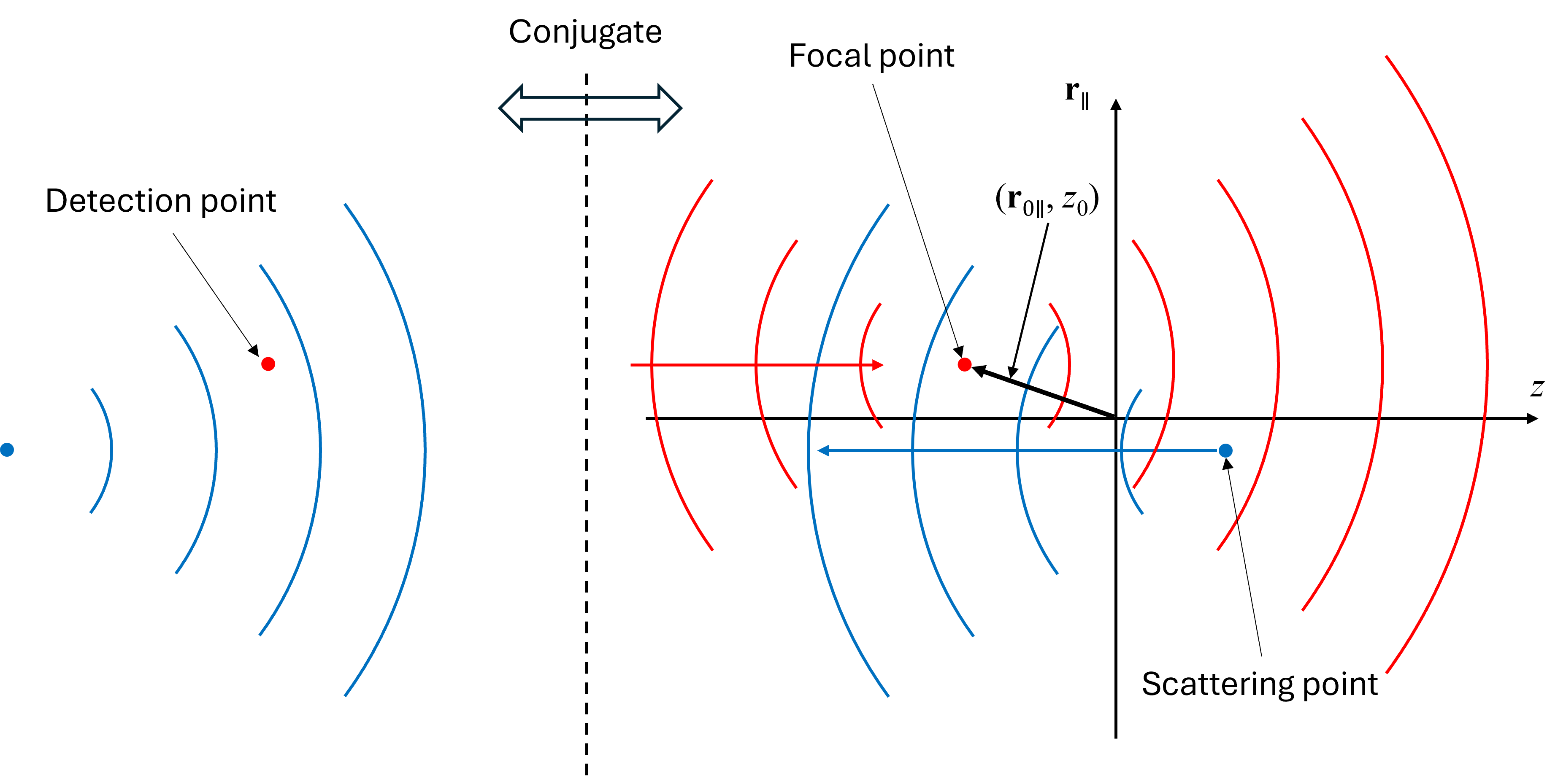
Figure 1: Schematic diagram describes the geometry of the illumination beam (red) focused at the red dot and backscattered wave (blue) from the blue dot.

Several previous works have formulated the image formation theory of OCT[20, 21, 22, 23]. Here in this paper, we reformulate the image formation theory of OCT with optical aberrations and for easy to interpret the computational method of OCT signal. We have started to formulate the imaging theory of the point-scanning FD-OCT system since it is the most common type among OCT systems. Other types of OCT systems can be obtained by modifying the illumination and collection configurations as shown in Sections LABEL:S-sec:CR_other_OCT. In the point-scanning FD-OCT (PSFD-OCT) system, the reflection confocal images interfered with the reference light are obtained at multiple optical frequencies. The detected light with 2D transversal scanning of the focused spot can be expressed as:

$$\begin{split}I(\mathbf{r}_{0\parallel},\omega;z_{0})=&\left\langle\left|\sqrt{p_{\mathrm{r}}S(\omega)}U_{\mathrm{r}}\mathrm{e}^{\mathrm{i}k_{\mathrm{r}}(\omega)l_{\mathrm{r}}}\right.\right.\\ &+\left.\left.\sqrt{pS(\omega)}\iiint h_{\mathrm{RCI}}(\mathbf{r}_{0\parallel}-\mathbf{r}_{\parallel},z_{0}-z,k_{\mathbf{s}}(\omega))\eta(\mathbf{r}_{\parallel},z,\omega)\mathrm{d}\mathbf{r}_{\parallel}\mathrm{d}z\right|^{2}\right\rangle_{D,t},\end{split}$$ (1)

where the time-dependent term $\mathrm{e}^{-\mathrm{i}\omega t}$ is omitted, and the bracket $\langle\cdot\rangle_{D,t}$ means the temporal and 2D spatial integration on the detection plane $D$, which is omitted hereafter. The unit of $I$ is [J$\cdot$Hz^-1]. $h_{\mathrm{RCI}}$ is the 3D complex point spread function (cPSF) of the reflection confocal imaging (RCI). $\eta$ is the scattering potential of the sample. $k_{\mathrm{s}}=n_{\mathrm{BG}}k$ is the wavenumber in the sample with the background refractive index $n_{\mathrm{BG}}$. The second term of the right-hand side of Eq. (1) is 3D spatial integration on $\mathbf{r}_{\parallel}$ and $z$. $\mathbf{r}_{0\parallel}=(x_{0},y_{0})$ is the transversal focal scanning location, $z_{0}$ is the axial location of the focus, $k$ is the optical wavenumber, $S$ is the spectral density of the light source [Hz^-1], and $p$, $p_{\mathrm{r}}$ are light power of the sample and reference arms, and $l_{\mathrm{r}}$ is the optical path length(OPL) of the reference arm respective to $z=0$. $U_{\mathrm{r}}$ is the monochromatic wave function of the reference light at the detector plane [m^-1]. Since both reference light and collected backscattered light are coupled into the same single-mode optical fiber, $U_{\mathrm{r}}$ is the same mode of the signal light; hence, it is a constant complex number. The wavenumber in a perfect dielectric medium $k(\omega)=\frac{\omega}{v_{\mathrm{p}}(\omega)}$ is a function of $\omega$, where $v_{\mathrm{p}}$ is the phase velocity of light. $k_{\mathrm{r}}$ is the wavenumber in the reference path. From hereafter, variable $\omega$ is dropped for simplicity. From these definitions, the cPSF $h_{\mathrm{RCI}}$ should have the unit [m^-2].

The scattering potential of the sample $\eta$ can be expressed as[24]:

$$\begin{split}\eta(\mathbf{r}_{\parallel},z,\omega)=&\frac{k^{2}(\omega)}{4\uppi}\left[n^{2}(\mathbf{r}_{\parallel},z,\omega)-n_{\mathrm{BG}}^{2}(\omega)\right]\\ =&\frac{k_{\mathrm{s}}^{2}(\omega)}{4\uppi}\chi_{\mathrm{p}}^{{}^{\prime}}(\omega)N(\mathbf{r}_{\parallel},z)-\frac{k_{\mathrm{s}}^{2}(\omega)}{4\uppi}\left[1-n_{\mathrm{BG}}^{-2}(\omega)\right],\end{split}$$ (2)

where $\chi_{\mathrm{p}}^{{}^{\prime}}=\frac{\chi_{\mathrm{p}}}{n_{\mathrm{BG}}^{2}}$, $\chi_{\mathrm{p}}$ is the molar dielectric susceptibility [m³], and $N$ is the density distribution of molecules that contribute to backscattering [m^-3]. The molar dielectric susceptibility $\chi_{\mathrm{p}}$ is related with refractive index as $n^{2}=1+\chi_{\mathrm{p}}N$. Here, the molar dielectric susceptibility $\chi_{\mathrm{p}}$ is assumed to be the same for all molecules of the scatterers. As we can see after, the spatial frequency component of the cPSF, $H_{\mathrm{RCI}}$ [Eq. (13)], is zero at 0 [m^-1]: $H_{\mathrm{RCI}}|_{\mathbf{f}=\mathbf{0}}=0$. Thus, the second term in Eq. (2), which is constant in space, can be ignored.

Here, we assume that each optical frequency channel detects a pure monochromatic wave. The interference signal is the cross-term of the right-hand side of Eq. (1) as:

$$\begin{split}I^{{}^{\prime}}(\mathbf{r}_{0\parallel},\omega;z_{0})=&\sqrt{pp_{\mathrm{r}}}S(\omega)\mathrm{e}^{-\mathrm{i}k_{\mathrm{r}}(\omega)l_{\mathrm{r}}}\\ &\times U_{\mathrm{r}}^{*}\iiint h_{\mathrm{RCI}}[\mathbf{r}_{0\parallel}-\mathbf{r}_{\parallel},z_{0}-z,k_{\mathbf{s}}(\omega)]\frac{k_{\mathrm{s}}^{2}(\omega)}{4\uppi}\chi_{\mathrm{p}}^{{}^{\prime}}(\omega)N(\mathbf{r}_{\parallel},z)\mathrm{d}\mathbf{r}_{\parallel}\mathrm{d}z\end{split}$$ (3)

Here, $I^{{}^{\prime}}$ is the complex-valued signal since its complex conjugate is ignored.

2.1 Complex point-spread function of reflection confocal imaging

The cPSF $h_{\mathrm{RCI}}$ expresses the collected light field by illuminating a point scatterer and collected by optics. The $h_{\mathrm{RCI}}$ is defined with the illumination field to the sample and collected filed mode of the backscattered field from the sample. Each step is described as follows.

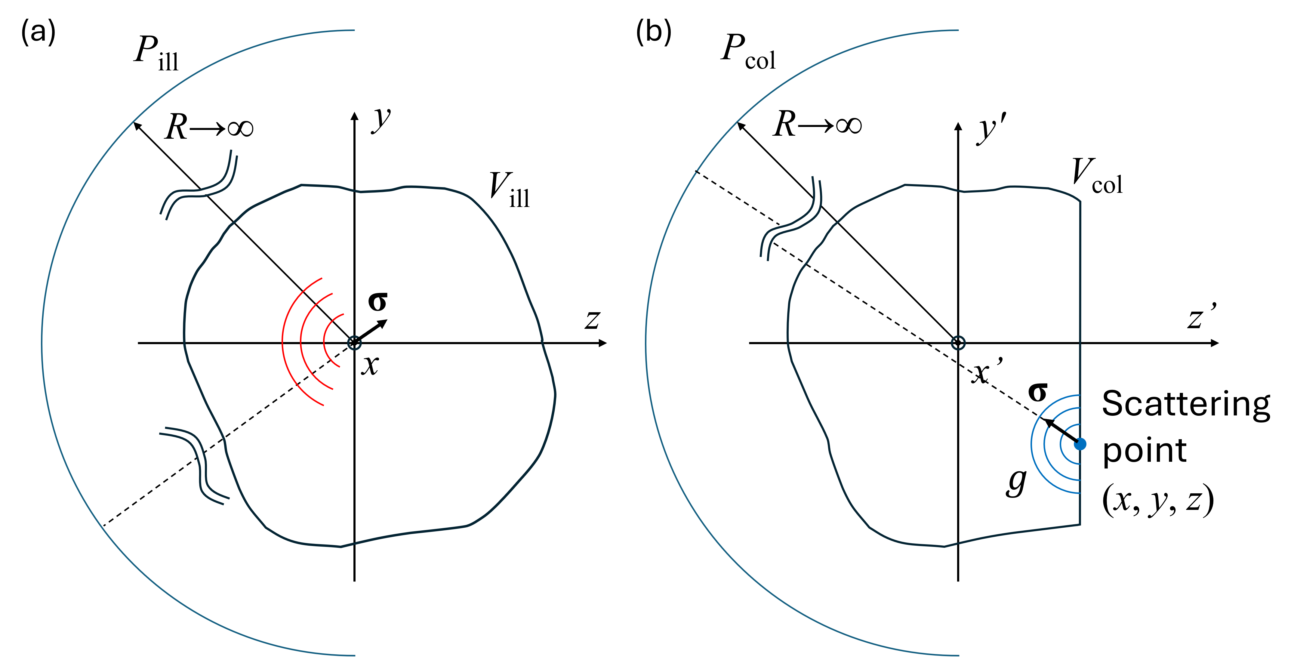
Figure 2: Definition of the space of (a) illumination and (b) collection fields.

2.1.1 Illumination field

The illumination field in the space $V_{\mathrm{ill}}$ to the sample [Figure 2(a)] can be expressed with a distribution $P_{\mathrm{ill}}$ on the sphere centered at the origin of $V_{\mathrm{ill}}$ with the Debye-Wolf integral[25] as:

$$f_{\mathrm{ill}}(\mathbf{r}_{\parallel},z,k)=\frac{\mathrm{i}k}{2\uppi}\iint P_{\mathrm{ill}}(-\bm{\upsigma}_{\parallel})\mathrm{e}^{\mathrm{i}k(\mathbf{r}_{\parallel}\cdot\bm{\upsigma}_{\parallel}+z\sigma_{z})}\mathrm{d}\Omega$$ (4)

where $\bm{\upsigma}_{\parallel}=(\sigma_{x},\sigma_{y})$, and $\sigma_{z}$ are directional cosines and $\sigma_{x}^{2}+\sigma_{y}^{2}+\sigma_{z}^{2}=1$. The unit vector $\bm{\upsigma}=(\sigma_{x},\sigma_{y},\sigma_{z})$ indicates the propagation direction of a plane wave component. Equation (4) is the summation of all plane wave components over solid angle $\Omega$ on the hemisphere with the radius $R$ [described as the blue curve in Figure 2(a)].

2.1.2 Backscattered field

The illumination filed $f_{\mathrm{ill}}$ is scattered by a scatterer located at $(\mathbf{r}_{\parallel},z)$. The scattered field at $\left(\mathbf{r}_{\parallel}^{{}^{\prime}},z^{{}^{\prime}}\right)$ can be expressed as:

$$f_{\mathrm{s}}\left(\mathbf{r}_{\parallel}^{{}^{\prime}},z^{{}^{\prime}},k\right)=g\left(\mathbf{r}_{\parallel}^{{}^{\prime}}-\mathbf{r}_{\parallel},z^{{}^{\prime}}-z,k\right)f_{\mathrm{ill}}(\mathbf{r}_{\parallel},z,k)$$ (5)

where $g(\mathbf{r})=\mathrm{e}^{\mathrm{i}k|\mathbf{r}|}/|\mathbf{r}|$ is the scalar green function [Figure 2(b)]. If we consider only backscattered, far propagation modes, the green function can be replaced with backward far field modes only[26] by using Weyl’s identity.

$$\begin{split}f_{\mathrm{bs}}\left(\mathbf{r}_{\parallel}^{{}^{\prime}},z^{{}^{\prime}},k\right)&=\frac{\mathrm{i}k}{2\uppi}\iint\mathrm{e}^{\mathrm{i}k\left[\left(\mathbf{r}_{\parallel}^{{}^{\prime}}-\mathbf{r}_{\parallel}\right)\cdot\bm{\upsigma}_{\parallel}-\left(z^{{}^{\prime}}-z\right)\sigma_{z}\right]}\mathrm{d}\Omega f_{\mathrm{ill}}(\mathbf{r}_{\parallel},z,k)\\ &=\frac{\mathrm{i}k}{2\uppi}\iint\mathrm{e}^{\mathrm{i}k\left(\mathbf{r}_{\parallel}^{{}^{\prime}}\cdot\bm{\upsigma}_{\parallel}-z^{{}^{\prime}}\sigma_{z}\right)}\mathrm{e}^{\mathrm{i}k\left(-\mathbf{r}_{\parallel}\cdot\bm{\upsigma}_{\parallel}+z\sigma_{z}\right)}\mathrm{d}\Omega f_{\mathrm{ill}}(\mathbf{r}_{\parallel},z,k),\end{split}$$ (6)

where the sign of $\sigma_{z}$ is negative because of the backward propagation.

2.1.3 Collection of backscattered field

The collected light from the single scattering point, i.e., the cPSF of RCI $h_{\mathrm{RCI}}(\mathbf{r}_{0\parallel}-\mathbf{r}_{\parallel},z_{0}-z,k)$, is the backscattered field at the location conjugated to the detection point, i.e. $\mathbf{r}^{{}^{\prime}}=\mathbf{r}_{0}$, after weighting each plane wave mode with the collection function $P_{\mathrm{col}}$. Because Eqs. (4)-(6) are defined with $\mathbf{r}_{0}=\mathbf{0}$,

$$\begin{split}h_{\mathrm{RCI}}(\mathbf{0}-\mathbf{r}_{\parallel},0-z,k)=&\frac{\mathrm{i}k}{2\uppi}\iint P_{\mathrm{col}}\left(\bm{\upsigma}_{\parallel}\right)\mathrm{e}^{\mathrm{i}k(-\mathbf{r}_{\parallel}\cdot\bm{\upsigma}_{\parallel}+z\sigma_{z})}\mathrm{d}\Omega f_{\mathrm{ill}}(\mathbf{r}_{\parallel},z,k)\end{split}$$ (7)

Hence, the collected field near the focus can also expressed with the combination of plane waves (Debye diffraction integral) as the same as the illumination field:

$$f_{\mathrm{col}}(\mathbf{r}_{\parallel},z,k)=\frac{\mathrm{i}k}{2\uppi}\iint P_{\mathrm{col}}\left(\bm{\upsigma}_{\parallel}\right)\mathrm{e}^{\mathrm{i}k(-\mathbf{r}_{\parallel}\cdot\bm{\upsigma}_{\parallel}+z\sigma_{z})}\mathrm{d}\Omega.$$ (8)

2.1.4 Interpretation of the cPSF

According to the above Eqs. (7) and (8), the cPSF $h_{\mathrm{RCI}}$ can be described as:

$$\begin{split}h_{\mathrm{RCI}}(\mathbf{r}_{\parallel},z,k)=&f_{\mathrm{col}}(-\mathbf{r}_{\parallel},-z,k)f_{\mathrm{ill}}(-\mathbf{r}_{\parallel},-z,k)\\ =&\frac{-k^{2}}{4\uppi^{2}}\iint P_{\mathrm{col}}(\bm{\upsigma}_{\parallel})\mathrm{e}^{\mathrm{i}k(\mathbf{r}_{\parallel}\cdot\bm{\upsigma}_{\parallel}-z\sigma_{z})}\mathrm{d}\Omega\\ &\times\iint P_{\mathrm{ill}}(-\bm{\upsigma}_{\parallel})\mathrm{e}^{-\mathrm{i}k(\mathbf{r}_{\parallel}\cdot\bm{\upsigma}_{\parallel}+z\sigma_{z})}\mathrm{d}\Omega\end{split}$$ (9)

Here, $P_{\mathrm{ill}}$ and $P_{\mathrm{col}}$ are illumination and collection filed distributions on a spherical plane centered at the geometrical focus according to the definition of Debye diffraction integral and assumed to be independent of optical frequency $\omega$. i.e., the angular distribution of the illumination and collection fields are the same for all optical frequencies. $P_{\mathrm{ill}/\mathrm{col}}/R$ is the amplitude of wave function for monochromatic wave. Hence, $P_{\mathrm{ill}/\mathrm{col}}$ is unitless. Thus, the unit of $h_{\mathrm{RCI}}$ is [m^-2].

Note that the Debye diffraction integral is based on the approximation that the volume of interest is small compared to the radius of the sphere, $R$. When we consider $R$ to be infinitely large, as shown in Figure 2, Eqs. (4) and (8) are probably accurate[25] in the entire object spaces of illumination $V_{\mathrm{ill}}$ and collection $V_{\mathrm{col}}$. Here, the space $V_{\mathrm{col}}$ is bounded at the axial location of each emitter to define only the backscattered field. In this case, $P_{\mathrm{ill}}$ and $P_{\mathrm{col}}$ correspond to the infinitely distant distributions. If we can consider that the objective is a thin lens and has no chromatic aberrations, $P_{\mathrm{ill}}$ and $P_{\mathrm{col}}$ might be equivalent to the illumination distribution and collection mode expressed at the front focal plane of the objective, respectively.

2.1.5 Spatial frequency representation

The diffraction integrals in [Eqs. (4) and (8)] can be treated as 2D spatial Fourier transforms (Section LABEL:S-sec:2DFT_focused_field), the illumination and collection fields can be expressed using spatial frequency and inverse Fourier transform as:

$$\begin{split}f_{\mathrm{ill}}(\mathbf{r}_{\parallel},z,k)&=\mathrm{i}\frac{2\uppi}{k}\mathcal{F}^{-1}_{\mathbf{f}_{\parallel}}\left[\frac{P_{\mathrm{ill}}\left(-\frac{2\uppi}{k}\mathbf{f}_{\parallel}\right)}{\sigma_{z}\left(\frac{2\uppi}{k}\mathbf{f}_{\parallel}\right)}\mathrm{e}^{\mathrm{i}kz\sigma_{z}\left(\frac{2\uppi}{k}\mathbf{f}_{\parallel}\right)}\right](\mathbf{r}_{\parallel})\\ &=\mathrm{i}\frac{2\uppi}{k}f_{\mathrm{ill}}^{{}^{\prime}}(\mathbf{r}_{\parallel},z,k)\\ f_{\mathrm{col}}(\mathbf{r}_{\parallel},z,k)&=\mathrm{i}\frac{2\uppi}{k}\mathcal{F}^{-1}_{\mathbf{f}_{\parallel}}\left[\frac{P_{\mathrm{col}}\left(-\frac{2\uppi}{k}\mathbf{f}_{\parallel}\right)}{\sigma_{z}\left(-\frac{2\uppi}{k}\mathbf{f}_{\parallel}\right)}\mathrm{e}^{\mathrm{i}kz\sigma_{z}\left(-\frac{2\uppi}{k}\mathbf{f}_{\parallel}\right)}\right](\mathbf{r}_{\parallel})\\ &=\mathrm{i}\frac{2\uppi}{k}f_{\mathrm{col}}^{{}^{\prime}}(\mathbf{r}_{\parallel},z,k),\end{split}$$ (10)

where $\mathcal{F}^{-1}_{x}[f](\nu)$ is the inverse Fourier transform of the function $f$ from $x$-space to $\nu$-space, and

$$\sigma_{z}(\bm{\upsigma}_{\parallel})=\sqrt{1-|\bm{\upsigma}_{\parallel}|^{2}}.$$ (11)

Hence, $\sigma_{z}(-\bm{\upsigma}_{\parallel})=\sigma_{z}(\bm{\upsigma}_{\parallel})$. The lateral spatial frequency $\mathbf{f}_{\parallel}$ is the Fourier transform pair of $\mathbf{r}_{\parallel}$.

The lateral Fourier transform of RCI’s cPSF $\tilde{h}_{\mathrm{RCI}}$ is now can be expressed as a 2D convolution in the lateral spatial frequency space by using Eq. (10) as:

$$\begin{split}\tilde{h}_{\mathrm{RCI}}(\mathbf{f}_{\parallel},z,k_{\mathrm{s}})=&\mathcal{F}_{\mathbf{r}_{\parallel}}[h_{\mathrm{RCI}}(\mathbf{r}_{\parallel},z,k_{\mathrm{s}})](\mathbf{f}_{\parallel})\\ =&-\frac{4\uppi^{2}}{k_{\mathrm{s}}^{2}}\left[\tilde{f}_{\mathrm{ill}}^{{}^{\prime}}(-\mathbf{f}_{\parallel},-z,k_{\mathrm{s}})\otimes_{\mathbf{f}_{\parallel}}^{2}\tilde{f}_{\mathrm{col}}^{{}^{\prime}}(-\mathbf{f}_{\parallel},-z,k_{\mathrm{s}})\right](\mathbf{f}_{\parallel},z,k_{\mathrm{s}}),\end{split}$$ (12)

where $[f\otimes_{\mathbf{x}}^{n}g]$ is the nD convolution operation between $f$ and $g$ with respect to $\mathbf{x}$. Then, the 1D Fourier transform along $z$ of exponentials in Eq. (12) becomes a delta function as:

$$\begin{split}H_{\mathrm{RCI}}(\mathbf{f}_{\parallel},f_{z},k_{\mathrm{s}})=&-\frac{4\uppi^{2}}{k_{\mathrm{s}}^{2}}\left[F_{\mathrm{ill}}^{{}^{\prime}}(-\mathbf{f}_{\parallel},-f_{z},k_{\mathrm{s}})\otimes_{\mathbf{f}}^{3}F_{\mathrm{col}}^{{}^{\prime}}(-\mathbf{f}_{\parallel},-f_{z},k_{\mathrm{s}})\right](\mathbf{f}_{\parallel},f_{z},k_{\mathrm{s}}),\end{split}$$ (13)

The three-dimensional spatial Fourier transform of $h_{\mathrm{RCI}}$ is called the coherent transfer function (cTF) of RCI[27, 28]. Because the cPSF $h_{\mathrm{RCI}}$ has the unit of [m^-2], cTF $H_{\mathrm{RCI}}$ has the unit of [m]. For each $k$, Eq. (13) is a 3D convolution of spherical caps. This approach for image formation is used for wide range of microscopies[27, 28, 29]. As shown in examples of previous studies, the RCI’s cTF has a thickness along the axial frequency direction $f_{z}$. This is not really optimal for 3D object structure reconstruction in PSFD-OCT since some axial frequency components of the object are already integrated within the axial thickness of the cTF during the OCT detection process. And also, this is the source of the signal loss at defocus[21]. However, in the case of a fiber-optic system, the thickness is mitigated by apodized detection[28]. Because PSFD-OCT is usually based on fiber-optic system and low NA illumination/collection, the cTF is not be thick along $f_{z}$, as shown in Figure LABEL:S-fig:Validation-sim.

2.1.6 Re-definition of cPSF

From Eq. (12), cPSF of RCI can be re-described as:

$$\begin{split}h_{\mathrm{RCI}}^{{}^{\prime}}(\mathbf{r}_{\parallel},z,k)=&-\frac{k^{2}}{4\uppi^{2}}h_{\mathrm{RCI}}(\mathbf{r}_{\parallel},z,k)\\ =&f_{\mathrm{col}}^{{}^{\prime}}(-\mathbf{r}_{\parallel},-z,k)f_{\mathrm{ill}}^{{}^{\prime}}(-\mathbf{r}_{\parallel},-z,k),\end{split}$$ (14)

Then, Eq. (3) can be re-written as:

$$\begin{split}I^{{}^{\prime}}(\mathbf{r}_{0\parallel},\omega;z_{0})=&-\sqrt{pp_{\mathrm{r}}}S(\omega)\mathrm{e}^{-\mathrm{i}k_{\mathrm{r}}(\omega)l_{\mathrm{r}}}\\ &\times\uppi U_{\mathrm{r}}^{*}\iiint h_{\mathrm{RCI}}^{{}^{\prime}}(\mathbf{r}_{0\parallel}-\mathbf{r}_{\parallel},z_{0}-z,k_{\mathrm{s}}(\omega))\chi_{\mathrm{p}}^{{}^{\prime}}(\omega)N(\mathbf{r}_{\parallel},z)\mathrm{d}\mathbf{r}_{\parallel}\mathrm{d}z.\end{split}$$ (15)

The redefined cPSF $h_{\mathrm{RCI}}^{{}^{\prime}}$ based on the spatial frequency descriptions [Eqs. (14) and (10)] is convenient because it simplifies the description of the OCT signal.

2.1.7 Represnetation of systematic aberrations

In the case of high-order systematic aberrations exists, cPSF, $h_{\mathrm{RCI}}^{{}^{\prime}}$, may be expressed by substituting $P_{\mathrm{ill}}(\bm{\upsigma}_{\parallel})\rightarrow P_{\mathrm{ill}}(\bm{\upsigma}_{\parallel})\mathrm{e}^{\mathrm{i}kW_{\mathrm{ill}}(\bm{\upsigma}_{\parallel},k)}$ and $P_{\mathrm{col}}(\bm{\upsigma}_{\parallel})\rightarrow P_{\mathrm{col}}\mathrm{e}^{\mathrm{i}kW_{\mathrm{col}}(\bm{\upsigma}_{\parallel},k)}$, where $W_{\mathrm{ill}}$ and $W_{\mathrm{col}}$ are the wavefront errors for illumination and collection at the infinitesimally distant spherical plane as the reference except the defocus.

$$W(\bm{\upsigma}_{\parallel},k)\equiv\sum_{j}w_{j}(k)Z_{j}\left(\frac{\bm{\upsigma}_{\parallel}}{\sigma_{\parallel,\mathrm{c}}}\right),$$ (16)

where $Z_{j}$ is a Zernike polynomial, $w_{j}$ is the wavefront error coefficient expanded by the Zernike polynomial, and $j$ is the index of Zernike coefficients in the single indexing scheme[30]. $\sin^{-1}\sigma_{\parallel,\mathrm{c}}$ is the cut-off angle of the illumination or collection and $n\sigma_{\parallel,\mathrm{c}}$ is the cut-off NA. With the spatial frequency $\mathbf{f}_{\parallel}$, it can be represented as

$$W(\mathbf{f}_{\parallel},k)\equiv\sum_{j}w_{j}(k)Z_{j}\left(\frac{\frac{2\uppi}{k}\mathbf{f}_{\parallel}}{\sigma_{\parallel,\mathrm{c}}}\right).$$ (17)

Rigorously, the pupil $P$ or wavefront errors $W$ will depend on the scanning location $\mathbf{r}_{0\parallel}$ according to the beam scanning method. In the case of translational beam scanning [Figure LABEL:S-fig:Interpret_Aberrations(a) Fig. 2], the displacement of the scanning beam on the physical aperture is equivalent to the displacement of the aperture of the optical system. The same plane wave component will be suffered by different wavefront aberrations. Hence, $W$ becomes a function of $\mathbf{r}_{0\parallel}$ as $W(\mathbf{r}_{0\parallel})$.

On the other hand, the fan-beam scanning [Figure LABEL:S-fig:Interpret_Aberrations(b)](Fig. 3) tilts the beam wavefront at the physical aperture. Hence, $P$ becomes a function of $\mathbf{r}_{0\parallel}$ as $P(\mathbf{r}_{0\parallel})$.

Both cases, the cTF becomes the function of $\mathbf{r}_{0\parallel}$ as $h_{\mathrm{RCI}}(\mathbf{r}_{\parallel},z,k,\mathbf{r}_{0\parallel})$. To assume that the image is constructed by convolution of object structure and $h_{\mathrm{RCI}}$, the scanning range should be small enough to regard $h_{\mathrm{RCI}}$ as constant over the scanning range. The maximum of this range may define the acceptable scanning range for CAC.

It should be noted that the ocular aberrations $W_{\mathrm{ocular}}$ are usually defined as wavefront errors at the anterior part of the eye[30]. This corresponds to the plane just before the objective. The definition differs from that of $W$, as shown in [Figure LABEL:S-fig:Interpret_Aberrations(c)]. Hence, many studies about retinal imaging methods, such as adaptive optics imaging, and aberrometers of the eye, reported the aberrations defined at this plane. The different definitions with $W$ may make it impossible to compare the aberrations estimated by CAC with PSFD-OCT and ocular aberrations reported by other studies directly.

Chromatic aberrations may be considered by introducing optical-frequency-dependent terms by substituting $\mathbf{r}_{0\parallel}(\omega)$, $z_{0}(\omega)$ with $\mathbf{r}_{0\parallel}$, $z_{0}$ in Eq. (3). They are optical-frequency-dependent spatial shifts. Hence, they can be expressed with $\omega$-dependent phase terms in pupils, and hence $\tilde{f}(\mathbf{f}_{\parallel},z-\Delta z_{\mathrm{ch}}(\omega),k)\mathrm{e}^{\mathrm{i}2\uppi\Delta\mathbf{r}_{\parallel\mathrm{ch}}(\omega)\cdot\mathbf{f}_{\parallel}}$, where $\Delta\mathbf{r}_{\parallel\mathrm{ch}}$ and $\Delta z_{\mathrm{ch}}$ are transversal and longitudinal chromatic aberrations. Since the wavelength-sweeping type FD-OCT (swept-source OCT: SS-OCT) scan the optical frequency to obtain the delay profile of OCT signal (A-line), the motion of sample during the wavelength scan can be considered as the chromatic aberrations. These results add more detailed understanding of the motion artifacts of SS-OCT[31].

2.2 Complex OCT signal reconstruction

Here, the reconstructed OCT signal, i.e., the complex OCT signal in the spatial domain, is described using the above derivations. The 1D inverse Fourier transform of Eq. (15) along $\omega$ becomes the complex OCT signal.

$$\begin{split}s(\mathbf{r}_{0\parallel},\tau;z_{0})=&\int I^{{}^{\prime}}(\mathbf{r}_{0\parallel},\omega;z_{0})\mathrm{e}^{\mathrm{i}\tau\omega}\mathrm{d}\omega\\ =&-\uppi\sqrt{pp_{\mathrm{r}}}U_{\mathrm{r}}^{*}\iiint h_{\mathrm{OCT}}(\mathbf{r}_{0\parallel}-\mathbf{r}_{\parallel},z_{0}-z,\tau)N(\mathbf{r}_{\parallel},z)\mathrm{d}\mathbf{r}_{\parallel}\mathrm{d}z\end{split}$$ (18)

where $h_{\mathrm{OCT}}$ is the cPSF of the OCT signal. This can be described with Eq. (14) as:

$$h_{\mathrm{OCT}}(\mathbf{r}_{\parallel},z,\tau)=\int\chi_{\mathrm{p}}^{{}^{\prime}}(\omega)S(\omega)\mathrm{e}^{-\mathrm{i}k_{\mathrm{r}}(\omega)l_{\mathrm{r}}}h_{\mathrm{RCI}}^{{}^{\prime}}(\mathbf{r}_{\parallel},z,k_{\mathrm{s}}(\omega))\mathrm{e}^{\mathrm{i}\tau\omega}\mathrm{d}\omega$$ (19)

2.3 Simplified model of the OCT image formation

2.3.1 Paraxial approximation

The axial frequency thickness of RCI’s cTF becomes thicker as the NAs of illumination and collection fields increase. However, it also means that the axial imaging range of PSFD-OCT (depth of focus) becomes shallow. Hence, PSFD-OCT is commonly used in low NAs. In this case, paraxial approximation $|\bm{\upsigma}_{\parallel}|\ll 1$ may be valid. Then,

$$\begin{split}\sigma_{z}\approx&1-\frac{|\bm{\upsigma}_{\parallel}|^{2}}{2}\\ =&1-\alpha(k)\left|\mathbf{f}_{\parallel}\right|^{2},\end{split}$$ (20)

where

$$\alpha(k)=\frac{1}{2}\left(\frac{2\uppi}{k}\right)^{2}.$$ (21)

And, $f_{\mathrm{ill}}^{{}^{\prime}}$ and $f_{\mathrm{col}}^{{}^{\prime}}$ in Eq. (10) can be approximated as:

$$\begin{split}f_{\mathrm{ill}}^{{}^{\prime}}(\mathbf{r}_{\parallel},z,k)\approx&\mathrm{e}^{\mathrm{i}kz}\mathcal{F}^{-1}_{\mathbf{f}_{\parallel}}\left[\frac{P_{\mathrm{ill}}(-\frac{2\uppi}{k}\mathbf{f}_{\parallel})}{1-\alpha(k)\left|\mathbf{f}_{\parallel}\right|^{2}}\mathrm{e}^{-\mathrm{i}kz\alpha(k)|\mathbf{f}_{\parallel}|^{2}}\right](\mathbf{r}_{\parallel})\\ f_{\mathrm{col}}^{{}^{\prime}}(\mathbf{r}_{\parallel},z,k)\approx&\mathrm{e}^{\mathrm{i}kz}\mathcal{F}^{-1}_{\mathbf{f}_{\parallel}}\left[\frac{P_{\mathrm{col}}(-\frac{2\uppi}{k}\mathbf{f}_{\parallel})}{1-\alpha(k)\left|\mathbf{f}_{\parallel}\right|^{2}}\mathrm{e}^{-\mathrm{i}kz\alpha(k)|\mathbf{f}_{\parallel}|^{2}}\right](\mathbf{r}_{\parallel}),\end{split}$$ (22)

The lateral Fourier transform of RCI’s cPSF $\tilde{h}_{\mathrm{RCI}}^{{}^{\prime}}$ [Eq. (14)] with paraxial approximation is now can be expressed using Eq. (22) as:

$$\tilde{h}_{\mathrm{RCI}}^{{}^{\prime}}(\mathbf{f}_{\parallel},z,k_{\mathrm{s}})\approx\mathrm{e}^{-2\mathrm{i}k_{\mathrm{s}}z}\tilde{\Gamma}(\mathbf{f}_{\parallel},z,k_{\mathrm{s}})$$ (23)

where

$$\tilde{\Gamma}(\mathbf{f}_{\parallel},z,k_{\mathrm{s}}) \equiv \left[A_{\mathrm{ill}}\mathrm{e}^{\mathrm{i}\phi_{\mathrm{ill}}}\otimes_{\mathbf{f}_{\parallel}}^{2}A_{\mathrm{col}}\mathrm{e}^{\mathrm{i}\phi_{\mathrm{col}}}\right](\mathbf{f}_{\parallel},z,k_{\mathrm{s}}),$$ (24)

$$A(\mathbf{f}_{\parallel},k_{\mathrm{s}}) \equiv \frac{P\left(\frac{2\uppi}{k_{\mathrm{s}}}\mathbf{f}_{\parallel}\right)}{1-\alpha(k_{\mathrm{s}})|\mathbf{f}_{\parallel}|^{2}}$$ (25)

$$\phi(\mathbf{f}_{\parallel},z,k_{\mathrm{s}}) \equiv k_{\mathrm{s}}z\alpha(k_{\mathrm{s}})\left|\mathbf{f}_{\parallel}\right|^{2}.$$ (26)

$A$ and $\phi$ are $A_{\mathrm{ill}}$ or $A_{\mathrm{col}}$, and $\phi_{\mathrm{ill}}$ or $\phi_{\mathrm{col}}$, respectively.

2.3.2 Paraxial 2D cTF with aberrations

The case with high-order aberrations may be expressed with Eq. (22) by substituting $P_{\mathrm{ill}}\rightarrow P_{\mathrm{ill}}\mathrm{e}^{\mathrm{i}kW_{\mathrm{ill}}}$ and $P_{\mathrm{col}}\rightarrow P_{\mathrm{col}}\mathrm{e}^{\mathrm{i}kW_{\mathrm{col}}}$, where $W_{\mathrm{ill}}$ and $W_{\mathrm{col}}$ are the wavefront errors except for the defocus. $W_{\mathrm{ill}}$ and $W_{\mathrm{col}}$ may be conjugate to the wavefront aberrations at the front focal plane of the objective. The phase term Eq. (26) will be treated as:

$$\phi(\mathbf{f}_{\parallel},z,k_{\mathrm{s}})\rightarrow k_{\mathrm{s}}z\alpha(k_{\mathrm{s}})\left|\mathbf{f}_{\parallel}\right|^{2}+k_{\mathrm{s}}W(\mathbf{f}_{\parallel},k_{\mathrm{s}}).$$ (27)

$W$ is $W_{\mathrm{ill}}$ or $W_{\mathrm{col}}$. When the illumination optics and the collection optics are identical, such as in the case of conventional fiber-optics-based PSFD-OCT, It can be regarded as $A_{\mathrm{ill}}=A_{\mathrm{col}}$ and $W_{\mathrm{ill}}=W_{\mathrm{col}}$.

2.3.3 OCT signal with paraxial and narrow-band approximations

By substituting Eq. (23) into Eq. (19), the cPSF of OCT under paraxial approximation is obtained as:

$$h_{\mathrm{OCT}}(\mathbf{r}_{\parallel},z,\tau)\approx-\uppi\int S(\omega)\chi_{p}^{{}^{\prime}}(\omega)\Gamma\left(\mathbf{r}_{\parallel},z,k_{\mathrm{s}}(\omega)\right)\mathrm{e}^{-\mathrm{i}[2zk_{\mathrm{s}}(\omega)+l_{\mathrm{r}}k_{\mathrm{r}}(\omega)]}\mathrm{e}^{\mathrm{i}\tau\omega}\mathrm{d}\omega$$ (28)

where

$$\begin{split}\Gamma(\mathbf{r}_{\parallel},z,k)=&\mathcal{F}^{-1}_{\mathbf{f}_{\parallel}}\left[\tilde{\Gamma}(\mathbf{f}_{\parallel},z,k)\right](\mathbf{r}_{\parallel})\\ =&\mathcal{F}^{-1}_{\mathbf{f}_{\parallel}}\left[A_{\mathrm{ill}}(\mathbf{f}_{\parallel},k)\mathrm{e}^{\mathrm{i}\phi_{\mathrm{ill}}(\mathbf{f}_{\parallel},z,k)}\right](\mathbf{r}_{\parallel})\times\mathcal{F}^{-1}_{\mathbf{f}_{\parallel}}\left[A_{\mathrm{col}}(\mathbf{f}_{\parallel},k)\mathrm{e}^{\mathrm{i}\phi_{\mathrm{col}}(\mathbf{f}_{\parallel},z,k)}\right](\mathbf{r}_{\parallel}).\end{split}$$ (29)

According to Eqs. (14) and (24) and that the peak magnitude of $h_{\mathrm{RCI}}$ is roughly proportional to the wavenumber fron Eq. (LABEL:S-eq:anal-ctf-hemisphere), $|h_{\mathrm{RCI}}(0,0,k)|\propto k$, the peak magnitude of $\Gamma$ is roughly proportional to $k^{3}$. If we can assume that $\chi_{p}^{{}^{\prime}}$ is independent from $\omega$ as $\chi_{p}^{{}^{\prime}}(\omega)\sim\chi_{p}^{{}^{\prime}}(\omega_{\mathrm{c}})$, and the distribution shape of $\tilde{\Gamma}$ is independent from $\omega$ as $\Gamma\left(\mathbf{f}_{\parallel},z,k(\omega)\right)\sim k^{3}(\omega)\Gamma^{\prime}\left(\mathbf{f}_{\parallel},z;k(\omega_{\mathrm{c}})\right)$ (narrow-band and no-chromatic aberration approximation), Eq. (28) becomes

$$h_{\mathrm{OCT}}(\mathbf{r}_{\parallel},z,\tau)\approx-\uppi\chi_{p}^{{}^{\prime}}(\omega_{\mathrm{c}})\Gamma^{\prime}\left(\mathbf{r}_{\parallel},z;k_{\mathrm{s}}(\omega_{\mathrm{c}})\right)\int k_{\mathrm{s}}^{3}(\omega)S(\omega)\mathrm{e}^{\mathrm{i}[\tau\omega-2zk_{\mathrm{s}}(\omega)-l_{\mathrm{r}}k_{\mathrm{r}}(\omega)]}\mathrm{d}\omega$$ (30)

Eq. (30) is the frequently used form of the OCT’s point spread function where lateral and axial (delay) resolutions are separable. This is somehow reasonable approximation when there is no strong absorption peaks of the sample over the light source’s spectrum and because the high-frequency oscillation term according to $k_{\mathrm{s}}$, $\mathrm{e}^{-2\mathrm{i}k_{\mathrm{s}}z}$, is excluded from $\tilde{\Gamma}$ [Eq. (23)].

If there is no high-order ($\geq$ 2nd order) dispersion in the medium and the reference arm, the wavenumber around the optical frequency $\omega_{\mathrm{c}}$ can be regarded as:

$$\begin{split}k_{\mathrm{s}}(\omega)=&\frac{\omega_{\mathrm{c}}}{v_{\mathrm{p,BG}}(\omega_{\mathrm{c}})}+\frac{1}{v_{\mathrm{g,BG}}(\omega_{\mathrm{c}})}(\omega-\omega_{\mathrm{c}})\\ =&\left[n_{\mathrm{BG}}(\omega_{\mathrm{c}})-n_{\mathrm{g,BG}}(\omega_{\mathrm{c}})\right]\frac{\omega_{\mathrm{c}}}{c}+n_{\mathrm{g,BG}}(\omega_{\mathrm{c}})\frac{\omega}{c},\end{split}$$ (31)

and

$$\begin{split}k_{\mathrm{r}}(\omega)=&\frac{\omega_{\mathrm{c}}}{v_{\mathrm{p,r}}(\omega_{\mathrm{c}})}+\frac{1}{v_{\mathrm{g,r}}(\omega_{\mathrm{c}})}(\omega-\omega_{\mathrm{c}})\\ =&\left[n_{\mathrm{r}}(\omega_{\mathrm{c}})-n_{\mathrm{g,r}}(\omega_{\mathrm{c}})\right]\frac{\omega_{\mathrm{c}}}{c}+n_{\mathrm{g,r}}(\omega_{\mathrm{c}})\frac{\omega}{c},\end{split}$$ (32)

where $v_{\mathrm{p}}=\frac{c}{n}$, $v_{\mathrm{g}}=\frac{1}{\partial k/\partial\omega}$, and $n_{\mathrm{g}}=\frac{c}{v_{\mathrm{g}}}$ are the phase velocity, group velocity, and group index. Then, the Fourier transform of Eq. (30) is

$$\begin{split}\int k_{\mathrm{s}}^{3}(\omega)S(\omega)\mathrm{e}^{\mathrm{i}[\tau\omega-2zk_{\mathrm{s}}(\omega)-l_{\mathrm{r}}k_{\mathrm{r}}(\omega)]}\mathrm{d}\omega=&\mathrm{e}^{-\mathrm{i}\frac{\omega_{\mathrm{c}}}{c}\left\{\left[n_{\mathrm{BG}}(\omega_{\mathrm{c}})-n_{\mathrm{g,BG}}(\omega_{\mathrm{c}})\right]2z+\left[n_{\mathrm{r}}(\omega_{\mathrm{c}})-n_{\mathrm{g,r}}(\omega_{\mathrm{c}})\right]l_{\mathrm{r}}\right\}}\\ &\times\sum_{n=0}^{3}\left\{B_{n}\gamma\left[\frac{2}{c}\left(l-n_{\mathrm{g,BG}}(\omega_{\mathrm{c}})z\right)\right]\right\}\end{split}$$ (33)

where $\gamma(\tau)\propto\mathcal{F}_{\omega}[S(\omega)](\tau)$ is the temporal coherence function, and the operator $B_{n}$ is

$$B_{n}=\binom{3}{n}\left\{-\mathrm{i}\frac{n_{\mathrm{g,BG}}(\omega_{\mathrm{c}})}{c}\right\}^{n}\left\{\left[n_{\mathrm{BG}}(\omega_{\mathrm{c}})-n_{\mathrm{g,BG}}(\omega_{\mathrm{c}})\right]\frac{\omega_{\mathrm{c}}}{c}\right\}^{(3-n)}\frac{\partial^{n}}{\partial l^{n}}.$$ (34)

The single-pass optical path length (OPL) relative to the reference arm $l=\frac{c\tau-n_{\mathrm{g,r}}(\omega_{\mathrm{c}})l_{\mathrm{r}}}{2}$ is the coordinate of axial direction in OCT images. Usually, the spread of $\Gamma$ along $z$ (confocal gate) is considerably broader than that of $\gamma$ (coherence gate). Hence, Eq. (33) can be treated as the axial point-spread function of OCT. And only here can the naive assumption be made that the lateral and axial resolutions are separable. Thus, it requires the paraxial and narrow-band approximations. Usually, $\frac{\omega_{\mathrm{c}}}{c}$ exhibits a large value, and hence, the magnitude of Eq. (33) can be assumed to be $B_{0}|\gamma|$. Since $B_{0}$ is a constant, the magnitude of the axial point-spread function of OCT is proportional to the magnitude of the temporal coherence function $|\gamma|$.

The axial point spread function is different from that of Villiger and Lasser[21], while they reported as $\mathcal{F}_{\omega}[k(\omega)S(\omega)](\tau)$. The difference may be coming from that we took into account the $\omega$-dependent cTF size while assuming $P_{\mathrm{ill}/\mathrm{col}}(\bm{\upsigma}_{\parallel})$ is $\omega$-independent. This $\omega$-dependent cTF size provides the factor of $k^{2}$ (Eq. (LABEL:S-eq:anal-ctf-hemisphere)).

3 Design of computational refocusing and aberration correction based on the image formation theory

3.1 Computational refocusing

Based on the OCT image formation theory, correction methods of defocus can be discussed. Theoretically, the computational refocusing (CR) is correcting the effect due to the shape of the cTF. From Eq. (15), the en face 2D Fourier transform of the OCT interference signal can be rewritten using the cTF $H^{\prime}$ as:

$$\begin{split}\tilde{I}^{{}^{\prime}}(\mathbf{f}_{\parallel},\omega;z_{0})=&-\uppi\sqrt{pp_{\mathrm{r}}}U_{\mathrm{r}}^{*}\chi_{\mathrm{p}}^{{}^{\prime}}(\omega)S(\omega)\mathrm{e}^{-\mathrm{i}k_{\mathrm{r}}(\omega)l_{\mathrm{r}}}\\ &\times\int H_{\mathrm{RCI}}^{{}^{\prime}}(\mathbf{f}_{\parallel},f_{z},k_{\mathrm{s}}(\omega))\tilde{N}(\mathbf{f}_{\parallel},f_{z})\mathrm{e}^{\mathrm{i}2\uppi z_{0}f_{z}}\mathrm{d}f_{z},\end{split}$$ (35)

where $H_{\mathrm{RCI}}^{{}^{\prime}}$ and $\tilde{N}$ are the 3D spatial Fourier transform of $h_{\mathrm{RCI}}^{{}^{\prime}}$ and the object structure $N$, respectively. The integration over $z$ in Eq. (15) is converted to the inverse Fourier transform from $f_{z}$ to $z_{0}$ in Eq. (35). If we assume a point scatterer at the location of $\mathbf{r}_{\mathrm{s}}=(\mathbf{r}_{\mathrm{s}\parallel},z_{\mathrm{s}})$, $N(\mathbf{r}_{\parallel},z)\rightarrow\delta(\mathbf{r}_{\parallel}-\mathbf{r}_{\mathrm{s}\parallel},z-z_{\mathrm{s}})$ and $\tilde{N}(\mathbf{f}_{\parallel},f_{z})\rightarrow\mathrm{e}^{-\mathrm{i}2\uppi\mathbf{f}_{\parallel}\cdot\mathbf{r}_{\mathrm{s}\parallel}}\mathrm{e}^{-\mathrm{i}2\uppi f_{z}z_{\mathrm{s}}}$. Then, the frequency spectrum of the complex OCT signal at the location of the point scatterer can be expressed as:

$$\begin{split}\tilde{I}^{{}^{\prime}}(\mathbf{f}_{\parallel},\omega;z_{0},\mathbf{r}_{\mathrm{s}})=&-\uppi\sqrt{pp_{\mathrm{r}}}U_{\mathrm{r}}^{*}\chi_{\mathrm{p}}^{{}^{\prime}}(\omega)S(\omega)\mathrm{e}^{-\mathrm{i}k_{\mathrm{r}}(\omega)l_{\mathrm{r}}}\\ &\times\int H_{\mathrm{RCI}}^{{}^{\prime}}(\mathbf{f}_{\parallel},f_{z},k_{\mathrm{s}}(\omega))\mathrm{e}^{-\mathrm{i}2\uppi\mathbf{f}_{\parallel}\cdot\mathbf{r}_{\mathrm{s}\parallel}}\mathrm{e}^{-\mathrm{i}2\uppi(z_{\mathrm{s}}-z_{0})f_{z}}\mathrm{d}f_{z},\end{split}$$ (36)

where $z_{\mathrm{s}}-z_{0}$ is the defocus distance at the location of the point scatterer, $\mathbf{r}_{\mathrm{s}}$. The phase errors of the OCT signal in the spatial frequency domain due to the defocus depends on the shape of the cTF.

Several methods for digital corrections of defocus have been proposed. Interferometric synthetic aperture microscopy (ISAM)[32] is a resampling of the data $\tilde{I}^{{}^{\prime}}$ in $(\mathbf{f}_{\parallel},\omega)$ space to retrieve the information in $(\mathbf{f}_{\parallel},f_{z})$ space. It is known that this requires an approximation in the case of PSFD-OCT[22]. ISAM assumes that $(\mathbf{f}_{\parallel},\omega)$ and $(\mathbf{f}_{\parallel},f_{z})$ spaces are bijective. Because the cTF of RCI is not infinitesimally thin along $f_{z}$, this is not valid, and hence, ISAM is not perfect correction rigorously. Theoretically, a low NA condition is required for ISAM to be a good approximation. Lee et al[33] show that ISAM becomes a phase-filtering method with a narrow-band approximation. Hence, under the narrow-band and paraxial approximations, ISAM becomes the forward-phase-filtering method[34].

Here we derive the forward-phase-filtering method from the image formation theory. Because the paraxial approximation and narrow-band approximation are required for the derivation, the descriptions are based on Eqs. (24)-(26).

In the case of single-mode fiber-based system, the same optical fiber is used in illumination and collection paths and limit the propagation mode. Hence, $P_{\mathrm{ill}}$ and $P_{\mathrm{col}}$ can be assumed as the same Gaussian distribution. With the low numerical apertureand the narrow-band approximation, the magnitude distributions may be assumed as a 2D Gaussian function independent from the wavenumber, $A=A_{\mathrm{ill}}=A_{\mathrm{col}}=\mathrm{e}^{-|\mathbf{f}_{\parallel}|^{2}/\Delta f^{2}}$. If there is only the defocus, the phase term $\phi(\mathbf{f}_{\parallel},z,k_{\mathrm{s}}(\omega_{\mathrm{c}}))\rightarrow\frac{2\uppi^{2}}{n_{\mathrm{BG}}k_{\mathrm{c}}}z|\mathbf{f}_{\parallel}|^{2}$, where $k_{\mathrm{c}}$ is the central wavenumber of the light source in the vacuum. 2D lateral Fourier transform of Eq. (24) becomes

$$\tilde{\Gamma}(\mathbf{f}_{\parallel},z;k_{\mathrm{s}}(\omega_{\mathrm{c}}))=\frac{\uppi}{2}\frac{A^{1/2}(\mathbf{f}_{\parallel},k_{\mathrm{s}}(\omega_{\mathrm{c}}))}{1/\Delta f^{2}-\mathrm{i}\phi_{\mathrm{def}}z}\mathrm{e}^{\mathrm{i}\frac{\phi_{\mathrm{def}}}{2}z|\mathbf{f}_{\parallel}|^{2}},$$ (37)

where

$$\phi_{\mathrm{def}}(\omega_{\mathrm{c}})=k_{\mathrm{s}}(\omega_{\mathrm{c}})\alpha(k_{\mathrm{s}}(\omega_{\mathrm{c}}))$$ (38)

is the defocus phase factor. Hence, the phase-only refocus filter is

$$\tilde{\Gamma}^{-1}_{\mathrm{CR},\mathrm{PSFD}}(\mathbf{f}_{\parallel},z;k_{\mathrm{s}}(\omega_{\mathrm{c}}))=\mathrm{e}^{-\mathrm{i}\frac{\phi_{\mathrm{def}}}{2}z_{\mathrm{s}}(l)|\mathbf{f}_{\parallel}|^{2}},$$ (39)

where $z_{\mathrm{s}}(l)\equiv\frac{l-l_{0}}{n_{\mathrm{g,BG}}}$ and $l-l_{0}\approx n_{\mathrm{g,BG}}(\omega_{\mathrm{c}})z$ is the optical path length in the sample from the focus $z=z_{0}$. This is identical to that of Ref. [34]. Furthermore, this method is equivalent to assume that the cTF is a parabola in the spatial frequency domain and independent from the wavenumber:

$$H_{\mathrm{RCI}}^{{}^{\prime}}(\mathbf{f}_{\parallel},f_{z};\omega_{\mathrm{c}})\rightarrow K(\mathbf{f}_{\parallel})\delta\left(f_{z}+\frac{k_{\mathrm{s}}(\omega_{\mathrm{c}})}{2\uppi}\left[2-\frac{\alpha(k_{\mathrm{s}}(\omega_{\mathrm{c}}))}{2}\left|\mathbf{f}_{\parallel}\right|^{2}\right]\right).$$ (40)

The discrepancy of the real cTF from this shape should be the source of correction error.

It should be noted that the phase term of $\tilde{\Gamma}$ depends on the magnitude distributions of the pupils, $P_{\mathrm{ill}}$ and $P_{\mathrm{col}}$, because of the convolution in Eq. (24). The defocus phase of Ref. [34] is based on the fact that the illumination and collection paths are identical, and $A_{\mathrm{ill}}=A_{\mathrm{col}}$ is assumed as a Gaussian distribution. When the system condition is different from this assumption, the optimal refocusing filter should be different from Eq. (39).

If the detection is through a free-space and infinitesimally small pinhole, the collection pupil may be approximated as unity $A_{\mathrm{col}}=1$. Then, Eq. (24) becomes

$$\tilde{\Gamma}(\mathbf{f}_{\parallel},z;n_{\mathrm{BG}}k_{\mathrm{c}})=\frac{\uppi\mathrm{e}^{-\frac{\Delta f_{\mathrm{ill}}^{2}\phi_{\mathrm{def}}^{2}z^{2}}{1+4\Delta f_{\mathrm{ill}}^{4}\phi_{\mathrm{def}}^{2}z^{2}}|\mathbf{f}_{\parallel}|^{2}}}{1/(\Delta f_{\mathrm{ill}}^{2})-\mathrm{i}2\phi_{\mathrm{def}}z}\mathrm{e}^{\mathrm{i}\frac{1+2\Delta f_{\mathrm{ill}}^{4}\phi_{\mathrm{def}}^{2}z^{2}}{1+4\Delta f_{\mathrm{ill}}^{4}\phi_{\mathrm{def}}^{2}z^{2}}\phi_{\mathrm{def}}z|\mathbf{f}_{\parallel}|^{2}},$$ (41)

where $A_{\mathrm{ill}}=\mathrm{e}^{-\frac{|\mathbf{f}_{\parallel}|^{2}}{\Delta f_{\mathrm{ill}}^{2}}}$ and $\Delta f_{\mathrm{ill}}=\text{NA}_{\mathrm{ill}}^{(\mathrm{e}^{-1})}/\lambda_{\mathrm{c}}$. The phase error due to the defocus is no longer linear with the amount of defocus. When $\Delta f_{\mathrm{ill}}^{4}\phi_{\mathrm{def}}^{2}z^{2}\ll 1$ $\left[|z|\ll\frac{1}{\Delta f_{\mathrm{ill}}^{2}\phi_{\mathrm{def}}}\right]$, the phase error is close to the plane wave illumination case [Eq. (LABEL:S-eq:S3)]. In the opposite case $\Delta f_{\mathrm{ill}}^{4}\phi_{\mathrm{def}}^{2}z^{2}\gg 1$ $\left[|z|\gg\frac{1}{\Delta f_{\mathrm{ill}}^{2}\phi_{\mathrm{def}}}\right]$, the phase error is approaching that of Eq. (37). It would be worth to note that the quadratic phase error is not linear with the defocus distance $z$. This is because the illumination and collection cut-off NAs are different.

The phase-only refocus filter is probably:

$$\tilde{\Gamma}^{-1}_{\mathrm{CR},\mathrm{NAp}}(\mathbf{f}_{\parallel},l;n_{\mathrm{BG}}k_{\mathrm{c}})=\mathrm{e}^{-\mathrm{i}\frac{1+2\Delta f_{\mathrm{ill}}^{4}\phi_{\mathrm{def}}^{2}z_{\mathrm{s}}^{2}(l)}{1+4\Delta f_{\mathrm{ill}}^{4}\phi_{\mathrm{def}}^{2}z_{\mathrm{s}}^{2}(l)}\phi_{\mathrm{def}}|\mathbf{f}_{\parallel}|^{2}z_{\mathrm{s}}(l)}.$$ (42)

The issue of the distribution of $P_{\mathrm{ill}}$ and $P_{\mathrm{col}}$ is not only for the phase-based method. The shape of cTF depends on these distributions, hence, the optimal resampling positions for ISAM also vary when $P_{\mathrm{ill}}$ and $P_{\mathrm{col}}$ have different distributions[35].

Other examples of the CR filters for other illumination and collection configurations are described in Section LABEL:S-sec:CR_other_OCT.

3.2 Computational aberration correction

The previously existing CAC or computational adaptive optics (CAO) methods estimate phase errors in the spatial frequency components of OCT signals[13, 36, 37, 17, 38, 39]. This is perhaps good for full-filed swept-source OCT[36, 37] because the illumination is a plane wave. Hence, Pill is a delta function, and then, $\tilde{\Gamma}(\mathbf{f}_{\parallel},z,k)$ is equivalent to the collection pupil $A_{\mathrm{col}}\mathrm{e}^{\mathrm{i}\phi_{\mathrm{col}}}$ [Eq. (37)]. The phase errors of OCT signal in the spatial frequency domain would be $\phi_{\mathrm{col}}$. Otherwise, the phase errors of OCT signal in the spatial frequency domain would be the results of the convolution between $A_{\mathrm{ill}}\mathrm{e}^{\mathrm{i}\phi_{\mathrm{ill}}}$ and $A_{\mathrm{col}}\mathrm{e}^{\mathrm{i}\phi_{\mathrm{col}}}$, and hence, cross-talk between $\phi_{\mathrm{ill}}$ and $\phi_{\mathrm{col}}$ occurred[19]. Because the second-order phase error (defocus) in $\phi_{\mathrm{ill}}$ and $\phi_{\mathrm{col}}$ depend on the depth $z$, not only the second-order, but also other oders of the phase errors of OCT signal in the spatial frequency domain would also be depth-dependent. Hence, previous CAC or CAO for PSFD-OCT require depth-wise aberration estimation for accurate correction.

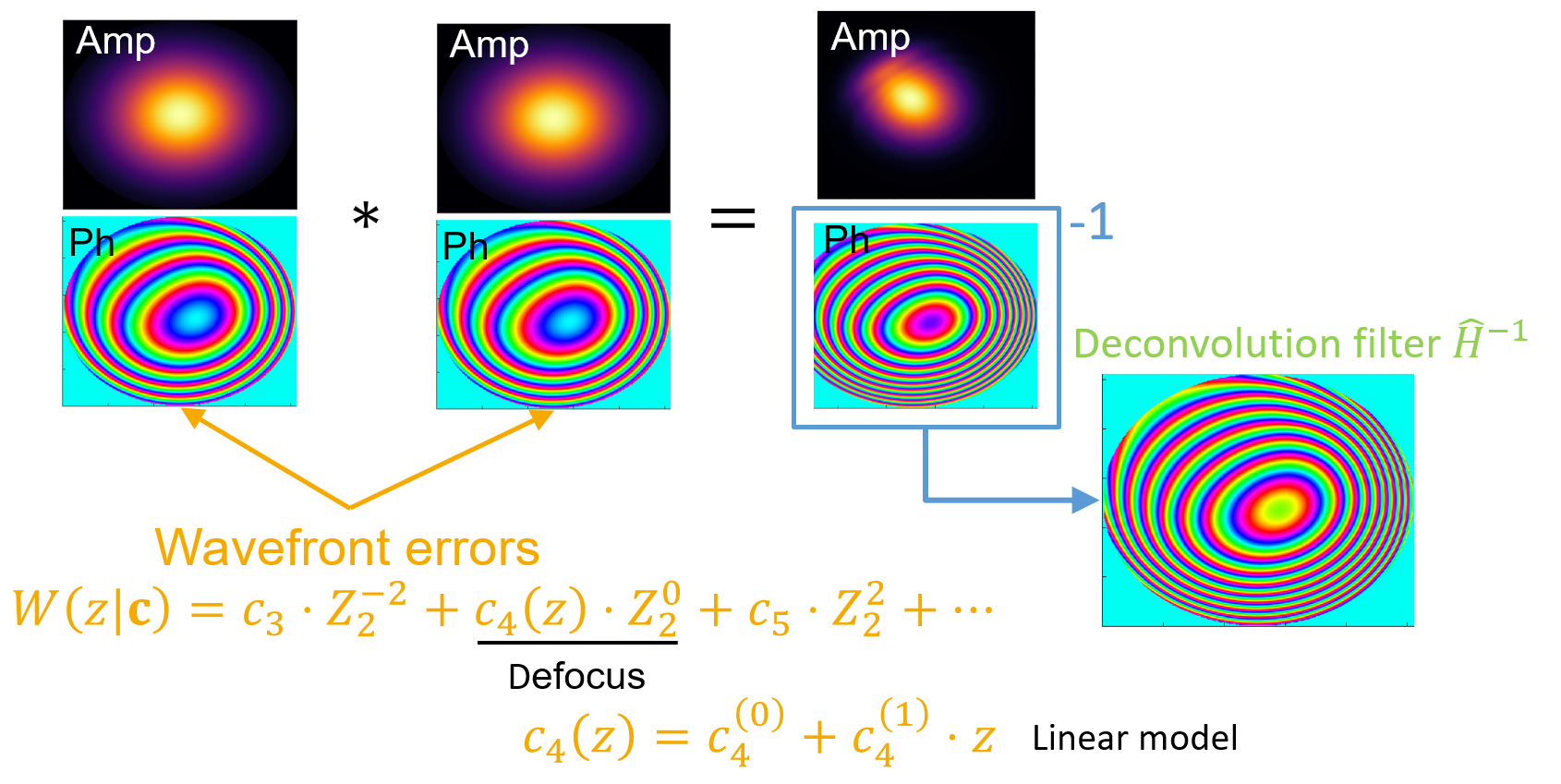
Figure 3: Schematic diagram of new CAC filter calculation.

In the case with the paraxial and narrow-band approximations, we can define the aberration correction filter based on Eq. (29). The schematic diagram to calculate the CAC filter is shown in Figure 3. The filter response in the spatial frequency domain can be defined with phase coefficients of Zernike polynomials, $\mathbf{c}={c_{j}}$, for wavefront aberrations in the pupil plane as:

$$\tilde{\Gamma}^{-1}_{\mathrm{CAC}}(\mathbf{f}_{\parallel},l,\mathbf{c})=\mathrm{e}^{-\mathrm{i}\arg[P^{\prime}\otimes_{\mathbf{f}_{\parallel}}^{2}P^{\prime}](\mathbf{f}_{\parallel};l,\mathbf{c})},$$ (43)

where

$$P^{\prime}(\mathbf{f}_{\parallel};l,\mathbf{c})=A^{\prime}(\mathbf{f}_{\parallel})\mathrm{e}^{\mathrm{i}\phi^{\prime}(\mathbf{f}_{\parallel},l,\mathbf{c})}.$$ (44)

$A^{\prime}$ and $\phi^{\prime}$ are the amplitude and phase of the expected aberrated pupil $P^{\prime}$. The inverse Fourier transform of Eq. (43), $\Gamma^{-1}$, corresponds to the inverse filter to cancel the broadening by aberrations. The pupil phase can be modeled as:

$$\phi^{\prime}(\mathbf{f}_{\parallel},l,\mathbf{c})=\sum_{j}c_{j}(l)Z_{j}\left(\frac{\mathbf{f}_{\parallel}}{f_{\mathrm{co}}/2}\right),$$ (45)

where $f_{\mathrm{co}}$ is the cut-off frequency of the OCT signal. According to Eq. (26), the coefficients $\mathbf{c}$ are expression of the wavefront aberrations with respective to the pupil plane $V$, and hence, only one coefficient of defocus $c_{4}$ will be depth-dependent. By comparing 4-th order Zernike polynomial in Eq. (45) with the defocus phase in Eq. (26),

$$c_{4}(l)Z_{4}\left(\frac{\mathbf{f}_{\parallel}}{f_{\mathrm{co}}/2}\right)=\phi_{\mathrm{def}}(\omega_{\mathrm{c}})z_{\mathrm{s}}(l)\left|\mathbf{f}_{\parallel}\right|^{2}+C(l),$$ (46)

where $C(l)$ is a constant phase in spatial frequency domain. Hence, it can be omitted. Since $Z_{4}(\bm{\rho})\equiv\sqrt{3}(2|\bm{\rho}|^{2}-1)$, we can define the $c_{4}$ as:

$$\begin{split}c_{4}(l)=&\frac{\phi_{\mathrm{def}}(\omega_{\mathrm{c}})(f_{\mathrm{co}}/2)^{2}}{2\sqrt{3}}\frac{l-l_{0}}{n_{\mathrm{g,BG}}}\\ \approx&\frac{\uppi\lambda_{0}(\omega_{\mathrm{c}})f_{\mathrm{co}}^{2}}{8\sqrt{3}n_{\mathrm{g,BG}}(\omega_{\mathrm{c}})n_{\mathrm{BG}}(\omega_{\mathrm{c}})}(l-l_{0}),\end{split}$$ (47)

where $\lambda_{0}(\omega)$ is the wavelength of the light with the frequency of $\omega$ in vacuum. Here, we assume that the optical path length is in proportion to the distance along the axial direction because of the paraxial and narrow-band approximations. This filter will be convolved with the OCT complex signal to cancel the aberration effects. The details of the implementation of this filter are described in the supplementary document.

By using this filter design, only single set of the polynomial coefficients, which describe the wavefront error with respective to the pupil plane $V$, can be used for the correction of the entire depth range.

The conventional CAC filter is based on the phase error estimation in the spatial frequency domain using Zernike polynomial directly.

$$\tilde{\Gamma}^{-1}_{\mathrm{CAC},\mathrm{conv}}(\mathbf{f}_{\parallel},l,\mathbf{a})=\mathrm{e}^{-\mathrm{i}\sum_{j}a_{j}(l)Z_{j}\left(\frac{\mathbf{f}_{\parallel}}{f_{\mathrm{co}}}\right)},$$ (48)

where $a_{j}(l)$ is the depth-dependent coefficients of Zernike polynomial. Only "de-focus" term $a_{4}(l)$ is depth-dependent, and the other terms are depth-independent.

$$\begin{split}a_{4}(l)=&\frac{k_{\mathrm{s}}(\omega_{\mathrm{c}})\alpha(k_{\mathrm{s}}(\omega_{\mathrm{c}}))f_{\mathrm{co}}^{2}}{2\times 2\sqrt{3}}z_{\mathrm{s}}(l)\\ \approx&\frac{\uppi\lambda_{0}(\omega_{\mathrm{c}})f_{\mathrm{co}}^{2}}{4\sqrt{3}n_{\mathrm{BG}}(\omega_{\mathrm{c}})n_{\mathrm{g,BG}}(\omega_{\mathrm{c}})}(l-l_{0}).\end{split}$$ (49)

This conventional method ignores the interaction of wavefront errors between the illumination and collection paths. And, simply assume that the phase error in OCT signal frequency due to HOAs is depth independent.

4 Numerical simulations

Here we show the numerical simulation results based on the image formation theory of OCT. Base on Eq. (18), the OCT signal is generated. The numerical simulation was validated b comparing with the simulated cTF and analytical obtained cTF [Figure LABEL:S-fig:Validation-sim]. Then, the CR and CAC filters are applied to the generated OCT signals.

4.1 Numerical simulation of computational refocusing

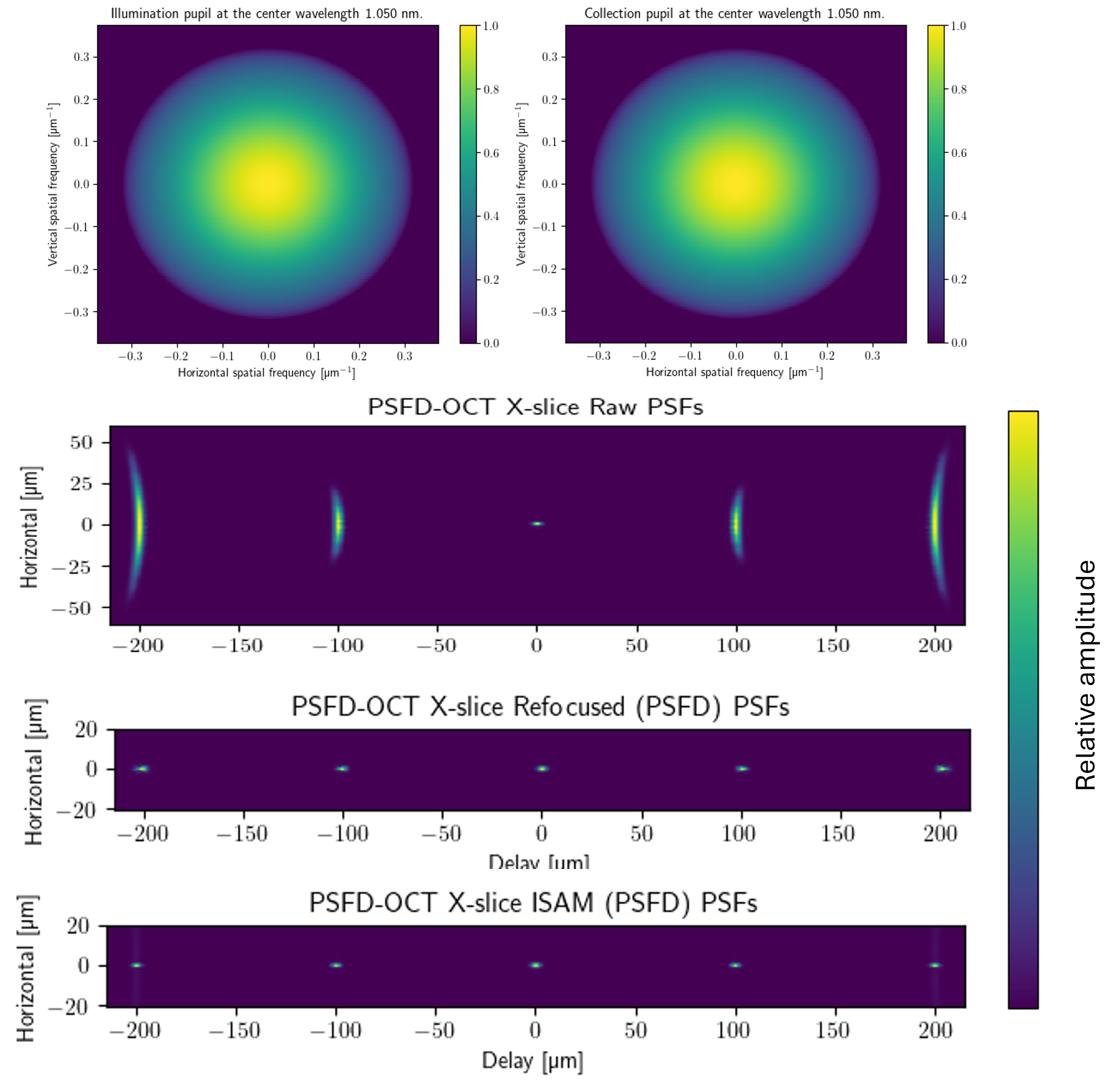
Figure 4: Numerical simulation of CR of PSFD-OCT.

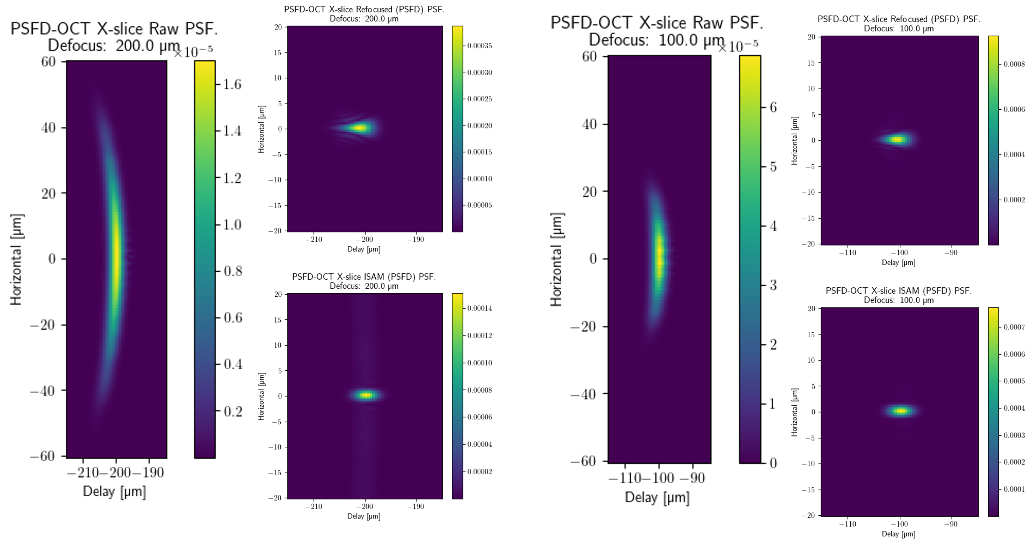
Figure 5: Numerical simulation of PSFs of PSFD-OCT with/without CR.

The simulated pupil amplitude $P_{\mathrm{ill}}$ and $P_{\mathrm{col}}$ at the central wavelength of 1,050 nm and PSFs with several defocus are shown in Figure 4, respectively. $P_{\mathrm{ill}}$ and $P_{\mathrm{col}}$ are the identical Gaussian distribution with cut-off NA of 0.25 and effective ($\mathrm{e}^{-1}$) NA of 0.2. No aberration $\mathbf{w}=\mathbf{0}$ is considered in this simulation. The CR filter [Eq. (39)] is applied to the simulated OCT signals. And ISAM[12] is also applied to the simulated OCT signals for comparison. Here, a simple implementation of ISAM [Section LABEL:S-sec:ISAM_PSFD] is used. Note that the amplitudes of PSFs are normalized to display the several defocused PSFs in the same scale. The enlarged PSFs with the defocus of 100 and 200 µm are shown in Figure 5.

With this NAs and defocus, the CR filter and ISAM can correct the defocus in similar performance in the lateral direction. In the axial direction, the CR filter cannot correct the axial elongation of the PSF because it is based on depth-by-depth correction. Hence, the slight axial elongation due to bending of PSFs with defocus is remained. On the other hand, ISAM can correct the axial elongation of the PSF because it is based on the resampling of the data in the three dimensional frequency domain $(\mathbf{f}_{\parallel},k)$. Fortunately, the axial elongation is not prominent due to low amplitudes of the PSFs at peripheral regions. In the case of the high NA, however, the axial elongation of the PSF is more prominent [Figs. LABEL:S-fig:PSFD-HighNA and LABEL:S-fig:PSFD_each-HighNA].

This numerical simulation shows that both CR filter and ISAM can correct the defocus in the PSFD-OCT with moderately high NAs well in the case of no HOAs.

4.2 Numerical comparison of computational aberration corrections

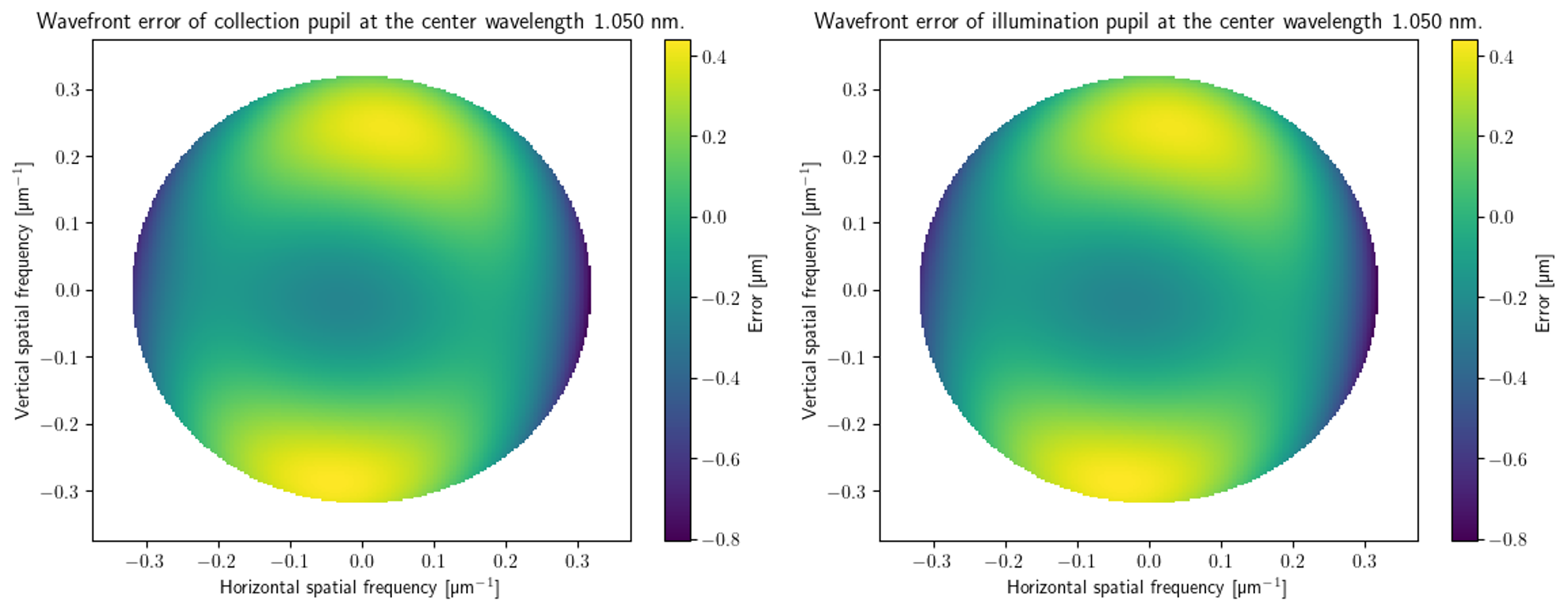
Figure 6: Numerically simulated aberrated pupil phases of PSFD-OCT. The identical aberrations for both pupils are assumed.

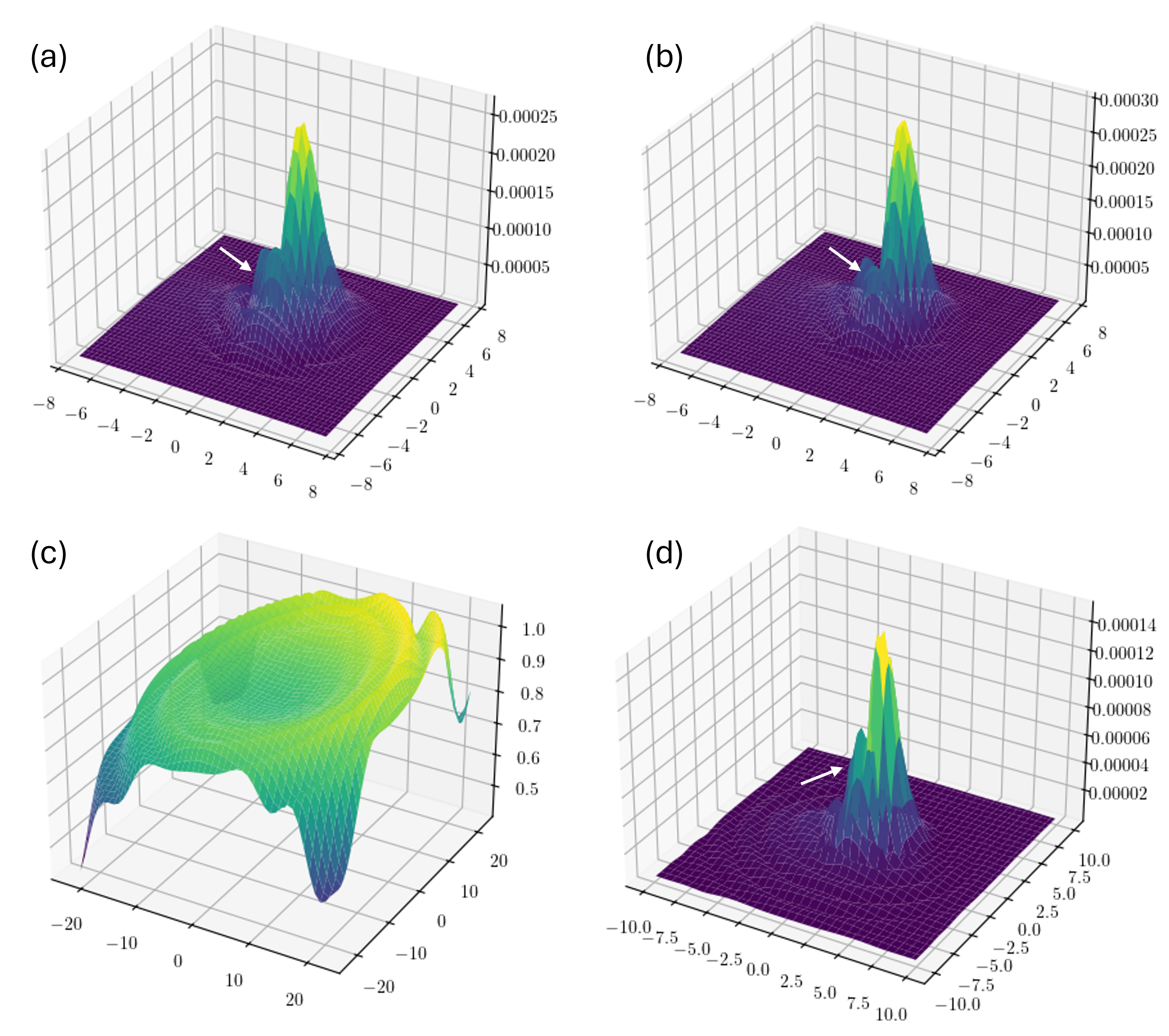
Figure 7: Numerical simulation of computational aberration correction of PSFD-OCT. PSFs aberration corrected with (a) conventional filter, (b) the designed filter, (c) without any correction, and (d) ISAM + HOPE correction are shown.

The numerical simulation of aberrated PSFD-OCT’s PSFs and corrected ones with the designed filter (Section 3.2) and conventional one are applied. The pupil size is the same to that of Section 4.1. High-order aberration (HOA) coefficients are set as, $w_{3}$: -0.05, $w_{5}$: 0.2, $w_{7}$: -0.032, $w_{8}$: 0.04, $w_{12}$: -0.1 µm. The simulated wavefront errors are shown in Figure 6.

The en face PSFs of the aberrated PSFD-OCT and corrected ones with the designed filter and conventional one are shown in Figure 7. The defocus amount is 200 µm. The designed filter [Eq. (43)] with the those setting coefficients of the defocus and HOAs at the central wavenumber of the light source has been applied. For the conventional filter [Eq. (48)], the simulated aberrated OCT PSF at in-focus is used to estimate the HOAs coefficients. The en face phase of spatial frequency of the in-focus PSF is fitted with the Zernike polynomials with the same order used in the designed filter. For comparison, the combination of ISAM and a high-order phase error (HOPE) correction [Eq. (48) with $a_{4}=0$] is also applied. This process is corresponding to the method of Ref. [13]. All filters can correct the defocus and HOAs somehow. However, the designed filter exhibits lower side lobes [Figure 7(b)] comparing to that of the conventional filter [Figure 7(a)] and ISAM + HOPE correction [Figure 7(d)]. This comparison show that the correction performance of the designed filter is slightly better than that of the conventional filter at this particular condition. Interestingly, the ISAM + HOPE correction shows poorer performance. Note that this comparison based on the perfect estimation of aberration coefficients. The iterative aberration estimate process for the real application (Section 6) is not included. Thus, this comparison does not include the adaption, i.e., fitting to signals, by optimization in iterative estimation.

5 Estimation procedure of aberration coefficients

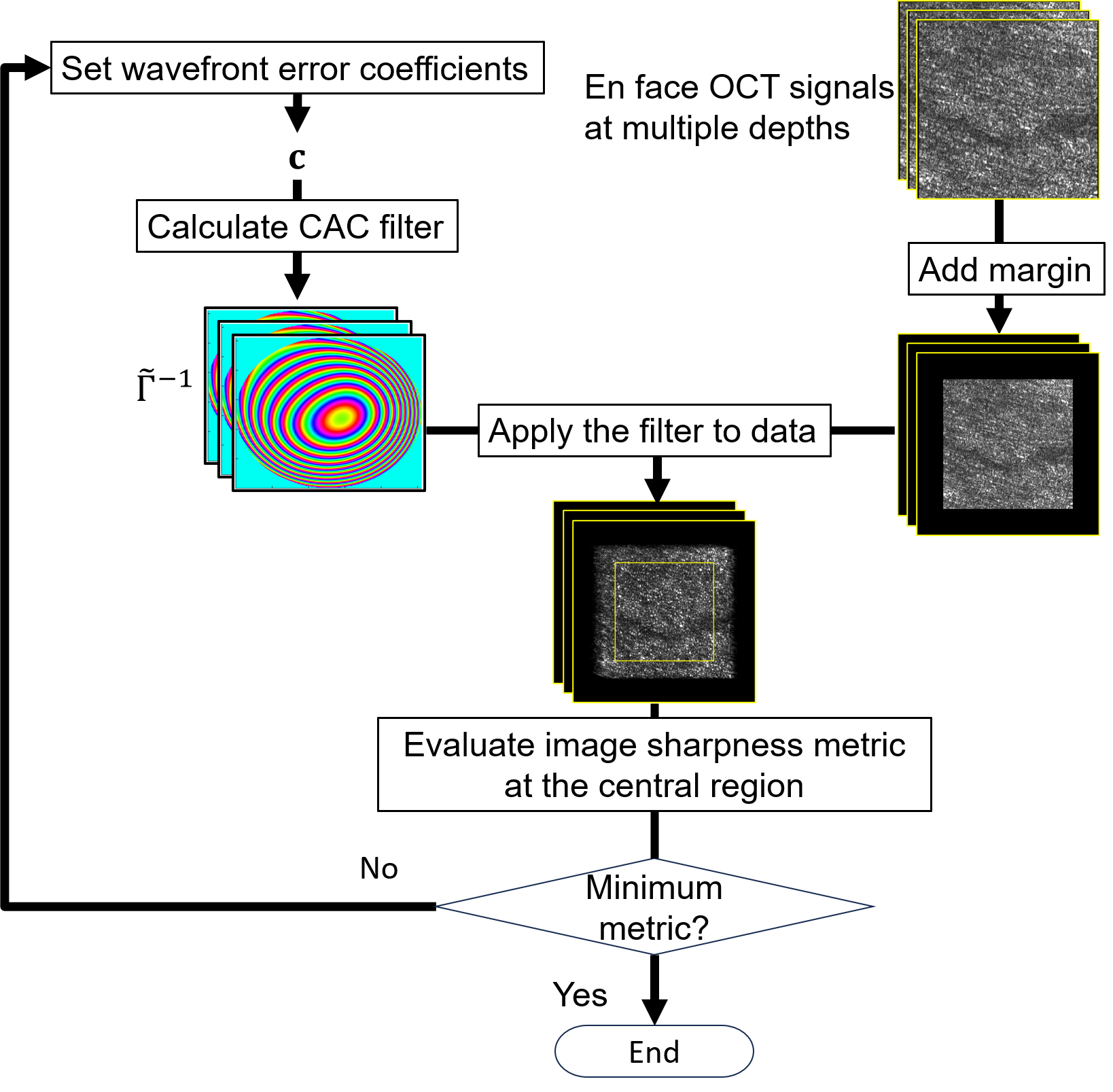
Figure 8: Schematic diagram of the procedure for estimating the wavefront error coefficients.

Before applying the CR and CAC filters to estimate or correct the OCT signals, the bulk phase shift correction for 2D en face plane phase error[40] is applied.

At first, the CR filter [Eq. (39)] is applied to estimate $l_{0}$ roughly. Then, CAC filter [Eq. (43)] is used to estimate coefficients of HOAs including $l_{0}$. The slope of $c_{4}$ along the depth is predefined using parameters $\lambda_{0}(\omega_{\mathrm{c}})$, $f_{\mathrm{co}}$, and $1/(n_{\mathrm{BG}}\times n_{\mathrm{g,BG}})=0.55$, which assuming the surrounding medium is water.

The schematic diagram of the procedure for estimating the wavefront error coefficients is shown in Figure 8. En face OCT signals at several depths are extracted from the volumetric data. The CAC filter is obtained by initial coefficients of HOAs and $l_{0}$. Then, the filter is applied to the selected en face signals and the image sharpness is assessed. The procedure is iterated to achieve the minimum metric value. The simplex algorithm (Nelder-Mead) is used for optimization. This is a robust algorithm and does not require derivatives[41]. Hence, relatively fast optimization can be achieved. However, the optimization is not stable in the case of high dimensional optimization. For the optimization including high-order aberrations, the “adaptive” option is used to improve the multi-dimensional optimization[42]. The parameters of the simplex algorithm are adapted for the dimension of problems.

The image sharpness is evaluated with the maximum-intensity-projection of OCT en face intensity images with few slices to suppress speckle patterns. The sharpness is assessed with the entropy-like metric[43]. The metric is assessed for each selected depth. Before obtaining a single value of the cost, metric values should be standardized at each depth. The optimization cost is now calculated as:

$$m^{{}^{\prime}}=\frac{1}{N}\sum_{i}^{N}\frac{m(l_{i})-m_{0}(l_{i})}{|m_{0}(l_{i})|}$$

, where $l_{i}$ is the optical path length at $i$-th extracted axial position, $m$ is the image metric value, and $m_{0}$ is the image metric value without correction.

For stable image sharpness assessment, edge margins are added to en face signals and a part of the central regions are used to calculate the sharpness metric. Since CR and CAC are signal convolution operation using Fourier transform, the boundary artifacts will occur. Zero-padding for all edges of en face images are applied[44, 45]. In addition, the performance near the edge is low because there is no signal outside the boundary that should contain part of the signal, which is necessary to recover the signal near the edge. Hence, the region of interest (ROI) for the image sharpness metric calculation was shrunk to exclude the region near the edge of image boundaries. These process are required to avoid the effects of the boundary in the image sharpness assessment.

6 Computational aberration correction of PSFD-OCT images

6.1 Phantom imaging

To confirm the aberration correction performance, a phantom experiment has conducted. The sample is a scattering phantom, where polystyrene microspheres were fixed by agar (1 µl volume of 1-µm diameter polystyrene microspheres and 6 ml of agar). We used 1.3 µm SS-OCT system[45, 46] for the phantom imaging. Briefly, it is a Jones-matrix (SS-OCT) setup at the central wavelength of 1.3-µm with a wavelength-swept light source with a 50-kHz sweeping rate. The objective is replaced with one have a short focal length (EFL=18 mm, LSM02, Thorlabs).T he effective numerical aperture (NA) is approximately 0.1. The diffraction-limited lateral resolution (1/e² diameter) at the focus is approximately 8.6 µm (in the air).

The raster scan with 300 × 300 A-lines has been applied. The scanning width was estimated with a grid pattern sample. The scanning area was approximately 643 × 579 µm. The sampling density will be 2.1 × 1.93 µm.

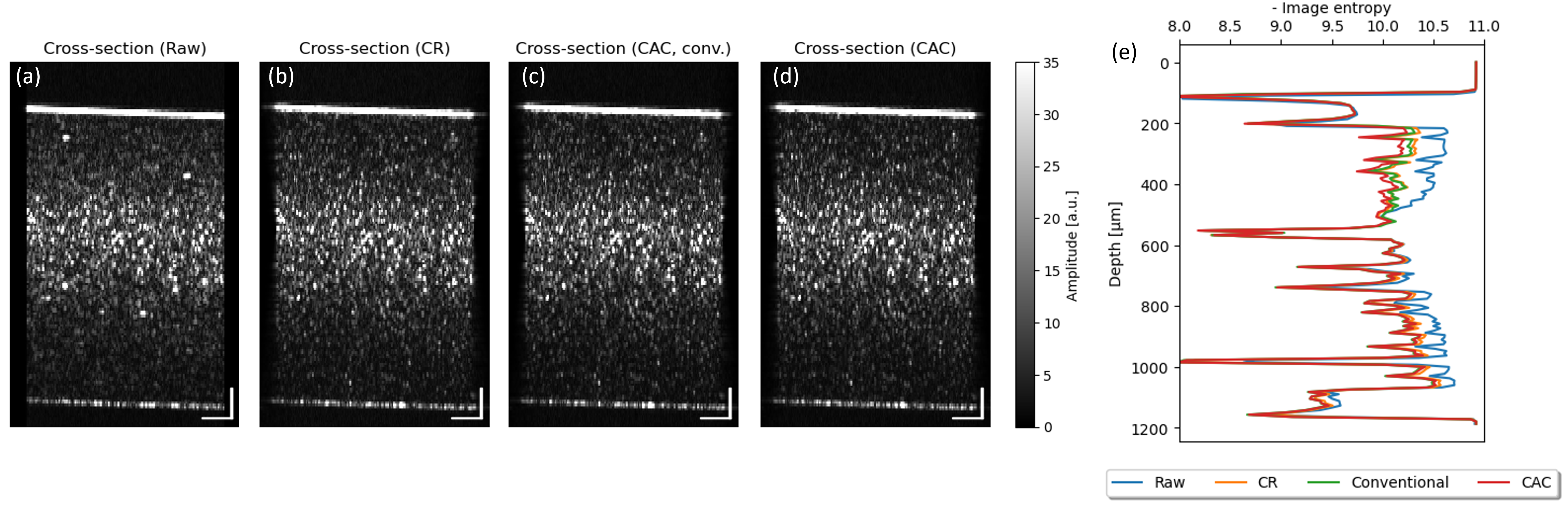
Figure 9: Microparticle phantom imaging with computational aberration correction.

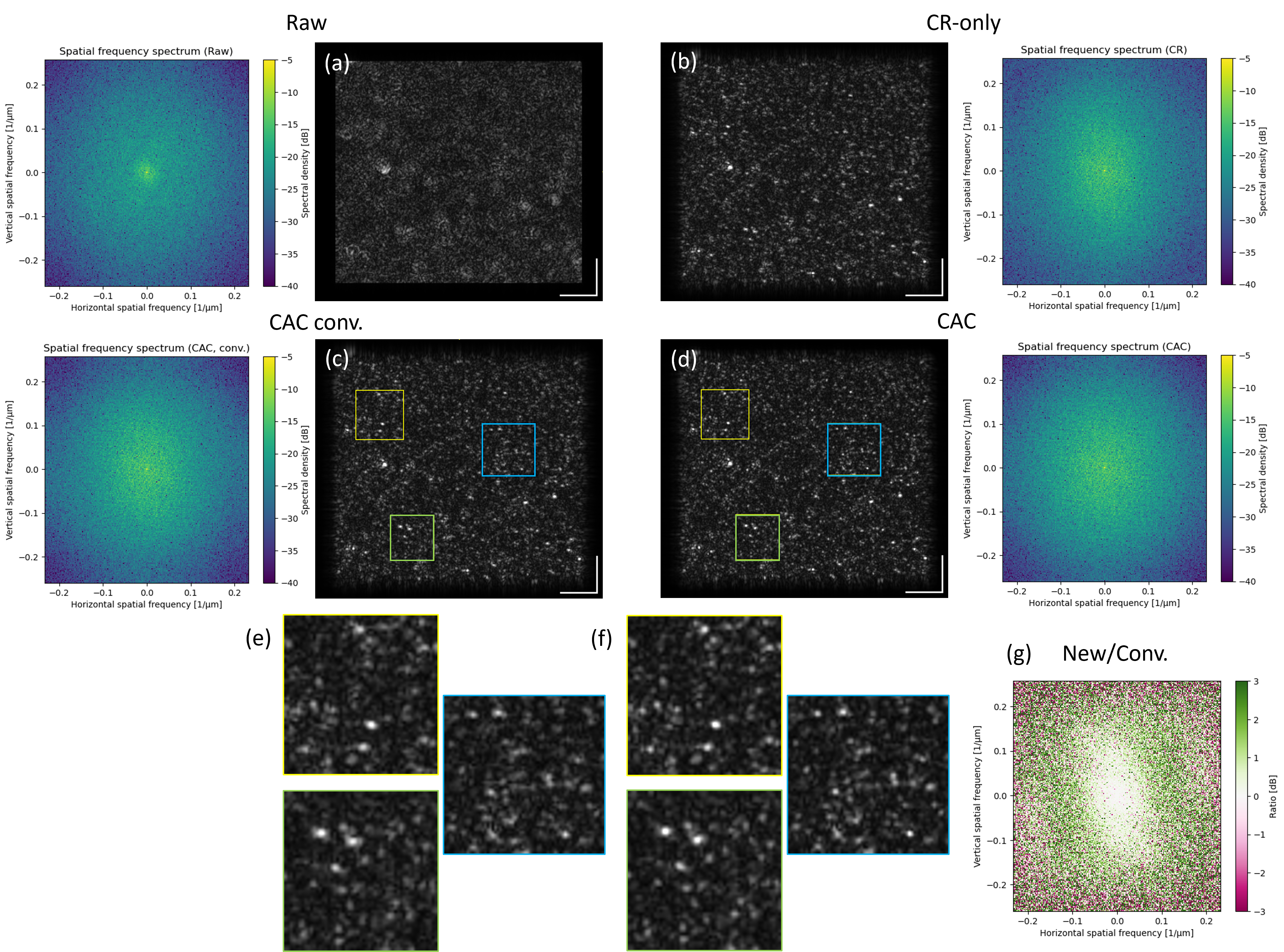
Figure 10: En face microparticle phantom images and spatial frequency spectrum with computational aberration correction.

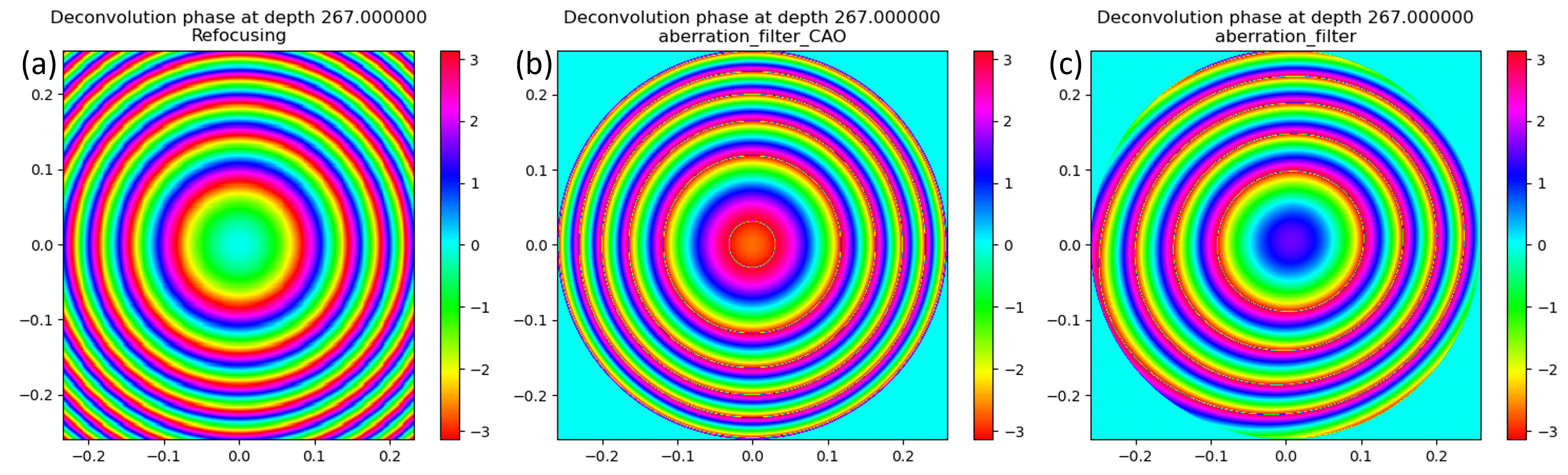
Figure 11: Correction filters used for en face microparticle phantom images (Figure 10).

The volumetric correction has been applied with both the new and conventional CAC filters. The new CAC and conventional CAC filters used the Zernike radial degree from 2 to 4, where $\mathbf{c}={c_{3},c_{4}(l),c_{5},c_{7},c_{8},c_{1}2}$ and $\mathrm{a}={a_{3},a_{4}(l),a_{5},a_{7},a_{8},a_{12}}$. Five en-face images were used for the estimation of coefficients. There are 6 (only offset for $c_{4}(l)$ and $a_{4}(l)$) coefficients in total.

The OCT intensity cross-sectional images of the microparticle phantom are shown in Figure 9. The CR-only image with the first step estimation () is also shown. The image sharpness metric of each depth is plotted in Figure 9(e). The new CAC filter shows the best performance in the image sharpness metric. Especially, the performance is better at the shallow depth. The conventional CAC filter exhibits slightly lower metric values compared to the CR filter.

The en face images of the microparticle phantom near the surface (depth: 253 µm) and their special frequency spectrum (intensity image, not complex signal) are shown in Figure 10. The en face images with the new filter (Figure 9d) exhibits slightly sharper particles compared to that with the conventional filter (Figure 9c). The enlarged panes of the en face images show the sharpness improvement clearly [Figs. 10(e) and 10(f)]. The ratio of the spatial frequency of images [Figure 10(g)] shows that the new filter has higher spatial frequency components compared to the conventional filter at peripheral frequencies. The used filters for correction at this depth (253 µm) are shown in Figure 11. The conventional CAC filter seems almost only the defocus is corrected. ($l_{0}$ = 579 [µm ], $a_{3}$ = -4.53 × 10^-5 [rad], $a_{5}$ = 1.95 × 10^-4 [rad], $c_{7}$ = -8.33 × 10^-6 [rad], $c_{8}$ = 1.38 × 10^-4 [rad], $c_{12}$ = -1.25 × 10^-4 [rad]). On the other hand, the new CAC filter have substantial HOAs coefficients. ($l_{0}$ = 546 [µm ], $c_{3}$ = -0.319 [rad], $c_{5}$ = 0.347 [rad], $c_{7}$ = -0.187 [rad], $c_{8}$ = -0.114 [rad], $c_{12}$ = -0.228 [rad]).

These suggest that the conventional filter requires depth-by-depth coefficients estimation for the best performance of CAC. On the other hand, the new filter can be performed good aberration correction of volumetric data with a single estimation. This is advantageous for the estimation time of coefficients with volumetric data.

6.2 In vivo retinal imaging

In vivo human retina has been imaged with 1-µm swept-source OCT system. Two configurations are used in this paper as mentioned following. The study was approved by the Institutional Review Boards of University of Tsukuba and adhered to the tenets of the Declaration of Helsinki. The nature of the present study and the implications of participating in this research project were explained to all study participants, and written informed consent was obtained from each participant before any study procedures or examinations were performed.

In the case of the in vivo retinal images, the retinal layer segmentation[47, 48, 49, 50] and sub-pixel registration among the B-scans are applied to flatten the volume at the retinal pigment epithelium line before applying the correction procedure described in Section 5.

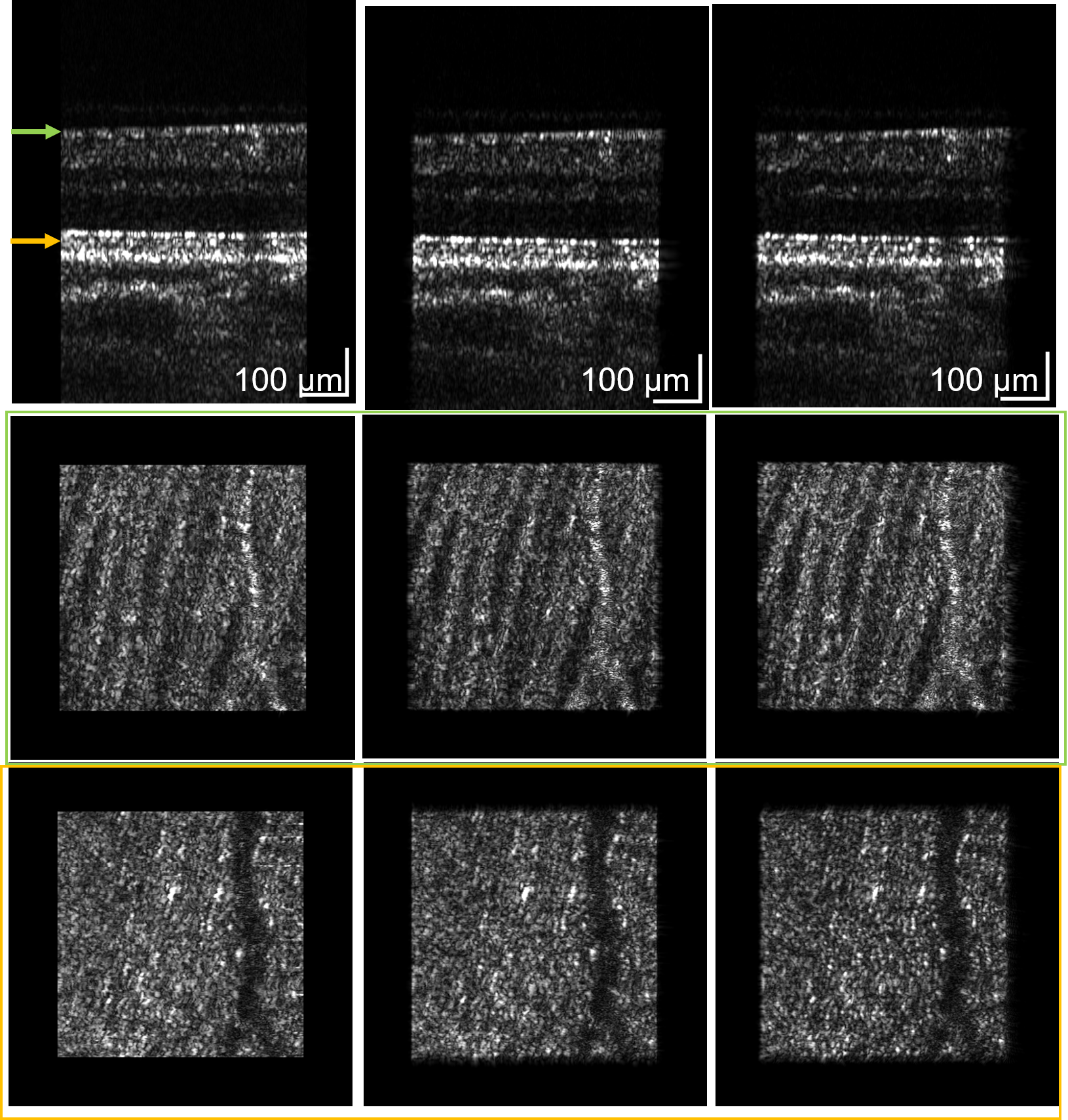
Figure 12: In vivo retinal imaging with computational aberration correction.

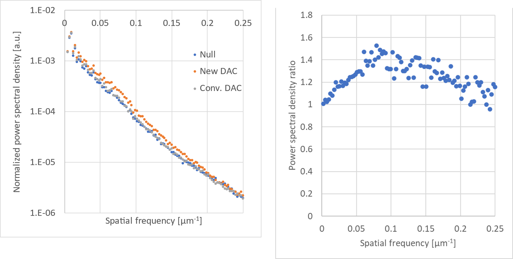
Figure 13: Spatial frequency spectrum of in vivo retinal imaging at the COST with computational aberration correction.

The scanning area is 500 µm. The CAC results of the retinal data are shown in Figure 12. The raster scan with 256 $\times$ 256 A-lines over 0.5 $\times$ 0.5 mm field of view was applied. A healthy volunteer’s right eye (43 yo) was scanned at around 4° temporal from the macula. The acquisition speed was 100 kHz, and the acquisition time was around 0.82 s. The beam diameter on the cornea was around 3.4 mm (1/e²), which corresponds to the effective numerical aperture in air of around 0.1. The illumination power is around 3.3 mW on the cornea, under the limit of the ANSI standard (Z80.36-2016). The high-order aberrations (HOA) from the 2nd to 4th radial order (12 coefficients) are taken into account. As shown in these results, the CAC shows finer structures compared to the direct estimation and correction.

The spatial frequency of the images was analyzed. En face OCT intensity images were 2D Fourier transformed, and 2D power spectra were obtained. Spectra were normalized by dividing each spectrum by the spectral density at 0 frequency. Then, the normalized spectra were averaged along the tangential direction to provide radial spatial frequency profiles. The radial spatial frequency profiles of photoreceptor en face images are shown in Figure 13. The ratio of radial frequency spectra of the new CAC over conventional CAC were calculated. Those also show that normalized spectral density at <0.2 [µm ^-1] are hight for the new CAC comparing to conventional CAC.

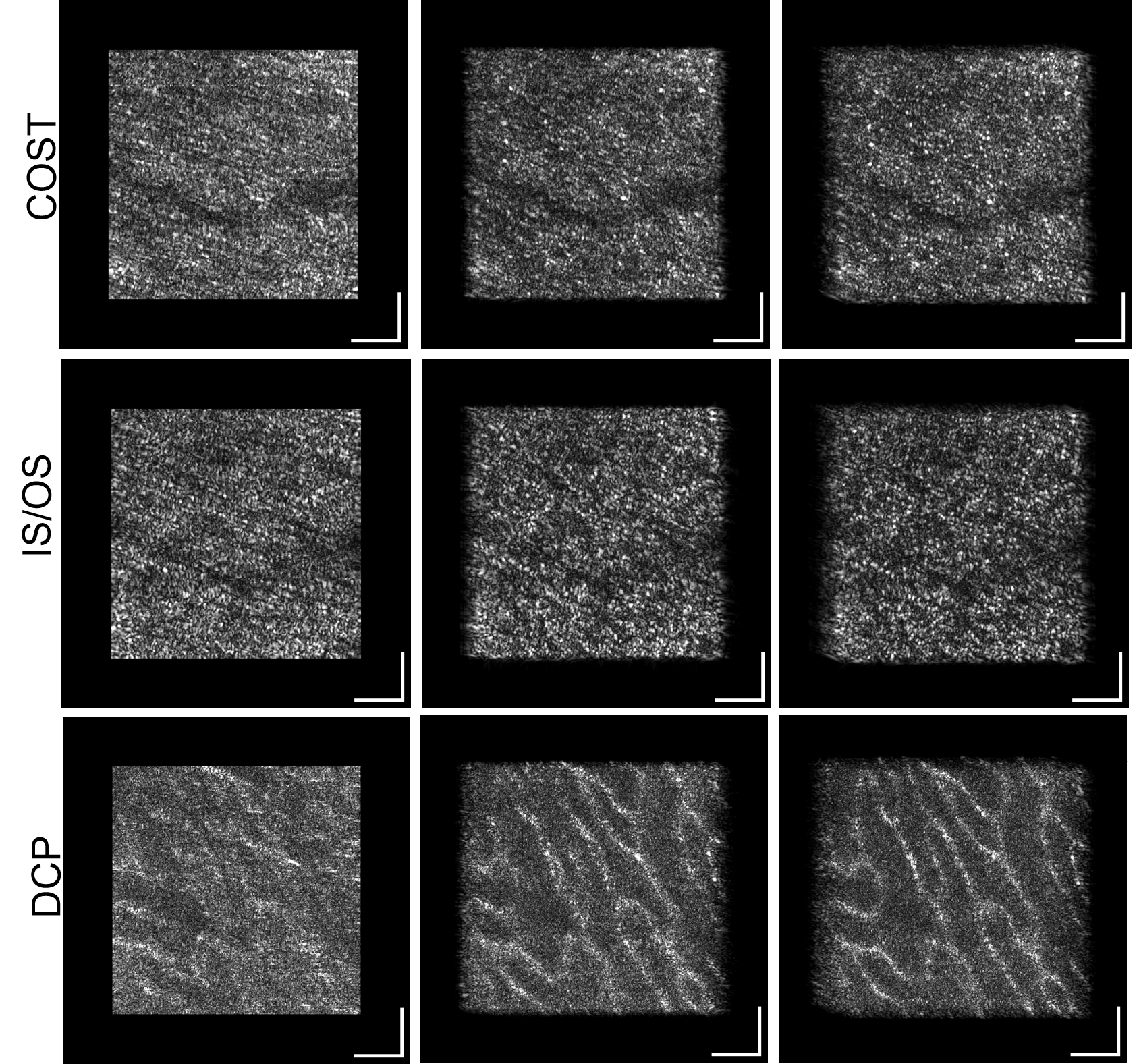
Figure 14: In vivo retinal imaging with computational aberration correction.

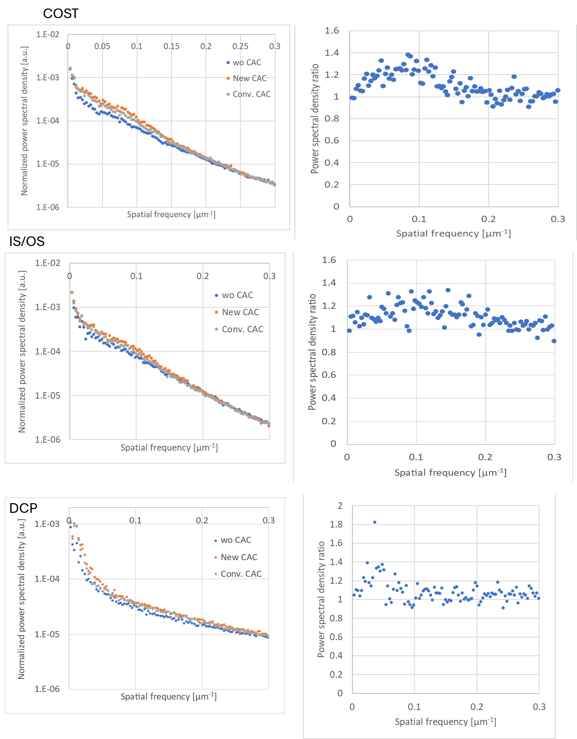
Figure 15: Spatial frequency spectrum of in vivo retinal imaging with computational aberration correction.

The other CAC results of the retinal data are shown in Figure 14. The raster scan with 300 $\times$ 300 A-lines over 0.5 $\times$ 0.5 mm field of view was applied. A healthy volunteer’s right eye (43 yo) was scanned at around 3° nasal from the macula. The acquisition speed was 200 kHz, and the acquisition time was around 0.56 s. The beam diameter on the cornea was around 5 mm (1/e²), which corresponds to the effective numerical aperture in air of around 0.15. The illumination power is around 2.2 mW on the cornea, under the limit of the ANSI standard (Z80.36-2016). The high-order aberrations (HOA) from the 2nd to 4th radial order (12 coefficients) are taken into account. As shown in these results, the CAC shows finer structures compared to the direct estimation and correction.

The spatial frequency of the images was analyzed. En face OCT intensity images were 2D Fourier transformed, and 2D power spectra were obtained. Spectra were normalized by dividing each spectrum by the spectral density at 0 frequency. Then, the normalized spectra were averaged along the tangential direction to provide radial spatial frequency profiles. The radial spatial frequency profiles of photoreceptor en face images are shown in Figure 15. The ratio of radial frequency spectra of the new CAC over conventional CAC were calculated. Those show that normalized spectral density at <0.2 [µm ^-1] are hight for the new CAC comparing to conventional CAC.

7 Discussion

7.1 Selection of computational aberration correction methods

The numerical simulation results suggest the brief guideline of the selection in the CR and CAC methods.

Although the ISAM for PSFD-OCTs is not the complete correction (Section 3.1), ISAM will works quite well with very high NAs in PSFD-OCT if there is only defocus (no HOAs) [Figs. LABEL:S-fig:PSFD-HighNA and LABEL:S-fig:PSFD_each-HighNA]. This is because the shape of the cTF is close to the ideal shape due to the Gaussian illumination and collection pupils.

The filtering method also restores the lateral resolution well in high NA cases, however, the axial resolution at out-of-focus cannot well achieved to the ideal one. This finding would be particularly important for judging the performance of CR in high NA cases. ALmost all previous CR works are assessing the lateral resolution, not axial resolution for evaluating the CR performance. If the horizontal resolution is the target of evaluation, the degradation of the axial resolution may be overlooked.

In the case of mild and low NAs ( 0.25), the filtering method works well [Figs.. 4 and 5]. Since filtering approach is rather simple and fast, it may be preferable for low-mild NA cases.

The situation is complex when there are both defocus and HOAs. They are interact with each other by the convolution of the illumination and collection pupils [Eq. (12)]. The filtering method designed in this manuscript seems to work well rather than conventional filtering method and ISAM + HOPE correction. Interaction of HOAs and defocus may cause the depth-dependent phase errors in the OCT signal. This would be the reason why the conventional filtering method for correcting all depth underscored to the designed filter. In addition, the cTF shape is also modulated irregularly by the interaction. This might be the issue in the case of using ISAM with HOAs since the ISAM is based on the shape of cTF. Furthermore, ISAM requires the knowledge of the focus depth position to remove the phase shift due to the offset of the focus [Section LABEL:S-sec:ISAM_implementation]. The focus depth estimation or iterative optimization of the ISAM respective to focus depth may be required. This becomes more difficult in cases where there are significant HOAs.

7.2 The limitation of the current computational aberration correction

The performance of the aberration correction is limited by several factors. The wavefront errors does not affect only the phase of the OCT spatial frequency signal, but also the amplitude. The convolution [Eq. (12)] of the aberrated pupils could results in the irregular shape of the spatial frequency gain of the OCT signal, $\left|\tilde{h}_{\mathrm{OCT}}\right|$, and hence, the irregular shape of the PSF. The de-convolution with modulating the amplitude of the spatial frequency components requires well-sophisticated regularization to avoid the generation of artifacts. For correction with the amplitude, it requires further development of the design of the CAC.

In addition, the amplitude of the pupils $P_{\mathrm{ill}}$ and $P_{\mathrm{col}}$ also affect the both of the amplitude and phase of the OCT spatial frequency components. In the application of CAC for PSFD-OCT (Section 6), the amplitude of the pupils are assumed to be a Gaussian distribution. If there is the discrepancy of the amplitude distributions from the Gaussian, the estimation of aberrations should have errors and the correction performance will be low. This suggests that the vignetting of the illumination and backscattered light should be avoided in order to achieve the best performance of the CAC with a priori knowledge of $P_{\mathrm{ill}}$ and $P_{\mathrm{ill}}$. This requirement might be especially important for in vivo retinal imaging.

The current design of the CAC is based on the paraxial and narrow-band approximations. The assumptions of the methods seem to be valid for the PSFD-OCT with the moderate NA such as in vivo retina case. In the case of optical coherence microscopy (OCM), the higher NA and broader spectral bandwidth will be used, and the assumptions would not be valid. However, if it is not the in vivo retinal imaging, the systematic optical aberrations could be suppressed by careful optical design or static correction optics. The current method may already be effective in correcting small residual systematic aberrations.

8 Conclusion

In this paper, we reformulated the image formation theory of OCT with systematic aberrations. The numerical investigated of computational refocusing in OCT shows that the refocusing of the PSFD-OCT works well with the CR filter up to, at least, moderately high NAs. In addition, it shows that the model-based design of CR filter by accounting the pupil amplitude distributions is important. The new CAC filter for PSFD-OCT has been designed based on the theory and it shows better aberration correction performance than the conventional CAC filter with in vivo retinal imaging. The same design approach may be used for other types of OCTs. The basic theory and the numerical simulation method will play an important role in the development of the computational aberration correction in OCTs.

Funding Core Research for Evolutional Science and Technology (JPMJCR2105); Japan Society for the Promotion of Science (21H01836, 21K09684, 22K04962).

Acknowledgments Please see https://optics.bk.tsukuba.ac.jp/COG/.

Disclosures

SM, LZ, YY: Topcon (F), Sky Technology (F), Nikon (F), Kao Corp. (F), Panasonic (F), Santec (F). NF: Nikon (E). L. Zhu is currently employed by Santec.

Data availability Data underlying the results presented in this paper are not publicly available at this time but may be obtained from the authors upon reasonable request.

Supplemental document See Supplement 1 for supporting content.

References

- [1] D. Huang, E. A. Swanson, C. P. Lin, et al., “Optical coherence tomography,” \JournalTitleScience 254, 1178–1181 (1991).
- [2] W. Drexler and J. G. Fujimoto, eds., Optical Coherence Tomography - Technology and Applications (Springer, 2015), 2nd ed.
- [3] J. M. Schmitt, S. L. Lee, and K. M. Yung, “An optical coherence microscope with enhanced resolving power in thick tissue,” \JournalTitleOpt. Commun. 142, 203–207 (1997).
- [4] F. Lexer, C. K. Hitzenberger, W. Drexler, et al., “Dynamic coherent focus OCT with depth-independent transversal resolution,” \JournalTitleJ. Mod. Opt. 46, 541–553 (1999).
- [5] M. Pircher, E. Götzinger, and C. K. Hitzenberger, “Dynamic focus in optical coherence tomography for retinal imaging,” \JournalTitleJ. Biomed. Opt. 11, 054013 (2006).
- [6] W. Drexler, U. Morgner, FX. Kartner, et al., “In Vivo ultrahigh-resolution optical coherence tomography,” \JournalTitleOpt. Lett. 24, 1221–1223 (1999).
- [7] J. P. Rolland, P. Meemon, S. Murali, et al., “Gabor-based fusion technique for Optical Coherence Microscopy,” \JournalTitleOpt. Express 18, 3632–3642 (2010).
- [8] M. Pircher and R. J. Zawadzki, “Combining adaptive optics with optical coherence tomography: Unveiling the cellular structure of the human retina in vivo,” \JournalTitleExpert Rev. Ophthalmol. 2, 1019–1035 (2007).
- [9] K. Kurokawa, Z. Liu, and D. T. Miller, “Adaptive optics optical coherence tomography angiography for morphometric analysis of choriocapillaris [Invited],” \JournalTitleBiomed. Opt. Express 8, 1803–1822 (2017).
- [10] K. Kurokawa, J. A. Crowell, N. Do, et al., “Multi-reference global registration of individual A-lines in adaptive optics optical coherence tomography retinal images,” \JournalTitleJ. Biomed. Opt. 26 (2021).
- [11] Y. Yasuno, Y. Sando, J.-i. Sugisaka, et al., “In-focus Fourier-domain Optical Coherence Tomography by Complex Numerical Method,” \JournalTitleOpt. Quant. Elect. 37, 1185–1189 (2005).
- [12] T. S. Ralston, D. L. Marks, P. S. Carney, and S. A. Boppart, “Inverse scattering for optical coherence tomography,” \JournalTitleJ. Opt. Soc. Am. A 23, 1027–1037 (2006).
- [13] S. G. Adie, B. W. Graf, A. Ahmad, et al., “Computational adaptive optics for broadband optical interferometric tomography of biological tissue,” \JournalTitleProc. Natl. Acad. Sci. U. S. A. 109, 7175–7180 (2012).
- [14] A. Kumar, W. Drexler, and R. A. Leitgeb, “Numerical focusing methods for full field OCT: A comparison based on a common signal model,” \JournalTitleOpt. Express 22, 16061–16078 (2014).
- [15] A. Kumar, W. Drexler, and R. A. Leitgeb, “Subaperture correlation based digital adaptive optics for full field optical coherence tomography,” \JournalTitleOpt. Express 21, 10850–10866 (2013).
- [16] N. D. Shemonski, F. A. South, Y.-Z. Liu, et al., “Computational high-resolution optical imaging of the living human retina,” \JournalTitleNat. Photonics 9, 440–443 (2015).
- [17] S. Ruiz-Lopera, R. Restrepo, C. Cuartas-Vélez, et al., “Computational adaptive optics in phase-unstable optical coherence tomography,” \JournalTitleOpt. Lett. 45, 5982–5985 (2020).
- [18] L. Ginner, A. Kumar, D. Fechtig, et al., “Noniterative digital aberration correction for cellular resolution retinal optical coherence tomography in vivo,” \JournalTitleOptica 4, 924–931 (2017).
- [19] F. A. South, Y.-Z. Liu, A. J. Bower, et al., “Wavefront measurement using computational adaptive optics,” \JournalTitleJ. Opt. Soc. Am. A 35, 466–473 (2018).
- [20] B. J. Davis, S. C. Schlachter, D. L. Marks, et al., “Nonparaxial vector-field modeling of optical coherence tomography and interferometric synthetic aperture microscopy,” \JournalTitleJ. Opt. Soc. Am. A 24, 2527–2542 (2007).
- [21] M. Villiger and T. Lasser, “Image formation and tomogram reconstruction in optical coherence microscopy,” \JournalTitleJ. Opt. Soc. Am. A 27, 2216–2228 (2010).
- [22] C. J. R. Sheppard, S. S. Kou, and C. Depeursinge, “Reconstruction in interferometric synthetic aperture microscopy: Comparison with optical coherence tomography and digital holographic microscopy,” \JournalTitleJ. Opt. Soc. Am. A 29, 244–250 (2012).
- [23] K. C. Zhou, R. Qian, A.-H. Dhalla, et al., “Unified k-space theory of optical coherence tomography,” \JournalTitleAdv. Opt. Photon. 13, 462–514 (2021).
- [24] Y. Sung, W. Choi, C. Fang-Yen, et al., “Optical diffraction tomography for high resolution live cell imaging,” \JournalTitleOpt. Express 17, 266–277 (2009).
- [25] J. Braat and P. Török, Imaging Optics (Cambridge University Press, Cambridge, 2019).
- [26] C. J. R. Sheppard, J. Lin, and S. S. Kou, “Rayleigh–Sommerfeld diffraction formula in k space,” \JournalTitleJ. Opt. Soc. Am. A 30, 1180–1183 (2013).
- [27] C. J. R. Sheppard, M. Gu, Y. Kawata, and S. Kawata, “Three-dimensional transfer functions for high-aperture systems,” \JournalTitleJ. Opt. Soc. Am. A 11, 593–598 (1994).
- [28] M. Gu, C. J. R. Sheppard, and X. Gan, “Image formation in a fiber-optical confocal scanning microscope,” \JournalTitleJ. Opt. Soc. Am. A 8, 1755–1761 (1991).
- [29] N. Fukutake, “A general theory of far-field optical microscopy image formation and resolution limit using double-sided Feynman diagrams,” \JournalTitleSci. Rep. 10, 17644 (2020).
- [30] L. N. Thibos, R. A. Applegate, J. T. Schwiegerling, and R. Webb, “Standards for Reporting the Optical Aberrations of Eyes,” \JournalTitleJ. Refract. Surg. 18, S652–S660 (2002).
- [31] S. H. Yun, G. J. Tearney, J. F. de Boer, and B. E. Bouma, “Motion artifacts in optical coherence tomography with frequency-domain ranging,” \JournalTitleOpt. Express 12, 2977–2998 (2004).
- [32] T. S. Ralston, D. L. Marks, P. Scott Carney, and S. A. Boppart, “Interferometric synthetic aperture microscopy,” \JournalTitleNat. Phys. 3, 129–134 (2007).
- [33] B. Lee, S. Jeong, J. Lee, et al., “Wide-Field Three-Dimensional Depth-Invariant Cellular-Resolution Imaging of the Human Retina,” \JournalTitleSmall 19, 2203357 (2023).
- [34] Y. Yasuno, J.-i. Sugisaka, Y. Sando, et al., “Non-iterative numerical method for laterally superresolving Fourier domain optical coherence tomography,” \JournalTitleOpt. Express 14, 1006–1020 (2006).
- [35] S. Coquoz, A. Bouwens, P. J. Marchand, et al., “Interferometric synthetic aperture microscopy for extended focus optical coherence microscopy,” \JournalTitleOpt. Express 25, 30807–30819 (2017).
- [36] D. Hillmann, H. Spahr, C. Hain, et al., “Aberration-free volumetric high-speed imaging of in vivo retina,” \JournalTitleSci. Rep. 6, 35209 (2016).
- [37] E. Auksorius, D. Borycki, P. Stremplewski, et al., “In Vivo imaging of the human cornea with high-speed and high-resolution Fourier-domain full-field optical coherence tomography,” \JournalTitleBiomed. Opt. Express 11, 2849–2865 (2020).
- [38] A. Kumar, L. M. Wurster, M. Salas, et al., “In-Vivo digital wavefront sensing using swept source OCT,” \JournalTitleBiomed. Opt. Express 8, 3369–3382 (2017).
- [39] A. Kumar, S. Georgiev, M. Salas, and R. A. Leitgeb, “Digital adaptive optics based on digital lateral shearing of the computed pupil field for point scanning retinal swept source OCT,” \JournalTitleBiomed. Opt. Express 12, 1577–1592 (2021).
- [40] K. Oikawa, D. Oida, S. Makita, and Y. Yasuno, “Bulk-phase-error correction for phase-sensitive signal processing of optical coherence tomography,” \JournalTitleBiomed. Opt. Express 11, 5886–5902 (2020).
- [41] J. A. Nelder and R. Mead, “A Simplex Method for Function Minimization,” \JournalTitleComput. J. 7, 308–313 (1965).
- [42] F. Gao and L. Han, “Implementing the Nelder-Mead simplex algorithm with adaptive parameters,” \JournalTitleComput Optim Appl 51, 259–277 (2012).
- [43] B. C. Flores, “Robust method for the motion compensation of ISAR imagery,” in Proc. SPIE, vol. 1607 D. P. Casasent, ed. (SPIE, Boston, MA, 1992), pp. 512–517.
- [44] M. Bertero and P. Boccacci, “A simple method for the reduction of boundary effects in the Richardson-Lucy approach to image deconvolution,” \JournalTitleA&A 437, 369–374 (2005).
- [45] L. Zhu, S. Makita, D. Oida, et al., “Computational refocusing of Jones matrix polarization-sensitive optical coherence tomography and investigation of defocus-induced polarization artifacts,” \JournalTitleBiomed. Opt. Express 13, 2975–2994 (2022).
- [46] E. Li, S. Makita, Y.-J. Hong, et al., “Three-dimensional multi-contrast imaging of in vivo human skin by Jones matrix optical coherence tomography,” \JournalTitleBiomed. Opt. Express 8, 1290–1305 (2017).
- [47] K. Li, X. Wu, D. Chen, and M. Sonka, “Optimal surface segmentation in volumetric images-A graph-theoretic approach,” \JournalTitleIEEE Trans. Pattern Anal. Mach. Intell. 28, 119–134 (2006).
- [48] M. Garvin, M. Abramoff, X. Wu, et al., “Automated 3-D intraretinal layer segmentation of macular spectral-domain optical coherence tomography images,” \JournalTitleIEEE Trans. Med. Imaging 28, 1436–1447 (2009).
- [49] M. Abramoff, M. Garvin, and M. Sonka, “Retinal Imaging and Image Analysis,” \JournalTitleIEEE Rev. Biomed. Eng. 3, 169–208 (2010).
- [50] B. Antony, M. D. Abràmoff, L. Tang, et al., “Automated 3-D method for the correction of axial artifacts in spectral-domain optical coherence tomography images,” \JournalTitleBiomed. Opt. Express 2, 2403–2416 (2011).