Binary Diffusion Probabilistic Model

Abstract

We introduce the Binary Diffusion Probabilistic Model (BDPM), a novel generative model optimized for binary data representations. While denoising diffusion probabilistic models (DDPMs) have demonstrated notable success in tasks like image synthesis and restoration, traditional DDPMs rely on continuous data representations and mean squared error (MSE) loss for training, applying Gaussian noise models that may not be optimal for discrete or binary data structures. BDPM addresses this by decomposing images into bitplanes and employing XOR-based noise transformations, with a denoising model trained using binary cross-entropy loss. This approach enables precise noise control and computationally efficient inference, significantly lowering computational costs and improving model convergence. When evaluated on image restoration tasks such as image super-resolution, inpainting, and blind image restoration, BDPM outperforms state-of-the-art methods on the FFHQ, CelebA, and CelebA-HQ datasets. Notably, BDPM requires fewer inference steps than traditional DDPM models to reach optimal results, showcasing enhanced inference efficiency.

1 Introduction

Generative models have become integral to advancements in modern machine learning, offering state-of-the-art solutions across various domains, including image synthesis, cross-modal tasks like text-to-image and text-to-video generation [33, 16]. Denoising diffusion probabilistic models (DDPMs) [37, 15] are particularly prominent within this landscape, utilizing iterative noise-based transformations to generate high-quality samples. These models predominantly employ Gaussian-based diffusion, which, while effective for continuous data, is less suited to inherently discrete or binary data representations. Despite diffusion models’ initial development for binary and categorical data [37], their adoption in these areas remains limited, leaving a gap for binary and discrete tasks in fields such as image processing and tabular data generation.

This paper introduces Binary Diffusion Probabilistic Model (BDPM), a novel approach specifically tailored to binary representation of essentially non-binary discrete data, which extends diffusion processes to better capture the characteristics of binary structures. Unlike traditional Gaussian DDPMs, that are applied to float representations of images, our BDPM model employs a bit-plane decomposition of images, representing pixel intensities as binary planes to enable a more efficient, interpretable generative process that aligns with the discrete nature of binary data. Additionally, BDPM integrates a binary cross-entropy loss function, offering a binary similarity metric that enhances training stability and model convergence.

Our contributions are as follows: (i) Novel Diffusion Generative Model: We propose BDPM, a diffusion-based generative model designed for binary data representations, optimized for the unique requirements of binary structures. (ii) State-of-the-Art Performance: BDPM demonstrates superior performance across multiple image restoration tasks, including super-resolution, inpainting, and blind image restoration, achieving competitive or improved results over existing state-of-the-art approaches, including Gaussian DDPM-based methods. (iii) Small Size Model. Our model with only 35.8M parameters, outperforms larger models, that are based often on large text-to-image models or pretrained on large-scale datasets, in terms of speed and performance. (iv) Enhanced Inference Efficiency: Our model attains high-quality results with a reduced number of sampling steps, leading to a more computationally efficient inference process compared to DDPMs.

By shifting from Gaussian to binary formulations in diffusion models, BDPM establishes a promising foundation for generative tasks where binary data representations are essential or beneficial from the computation and interpretation perspectives.

2 Related work

Traditional DDPMs. Denoising Diffusion Probabilistic Models (DDPMs) [37, 15] have become the go-to solutions in generative modeling in the last years. These models define a forward diffusion process that progressively adds scaled Gaussian noise ${\bm{\epsilon}}\sim\mathcal{N}({\bf 0},\mathbf{I})$ to data, transforming initially complex data distributions into a standard Gaussian distribution over multiple time steps. Specifically, the forward process is formulated as:

$$q(\mathbf{x}_{t}|\mathbf{x}_{t-1})=\mathcal{N}\left(\mathbf{x}_{t};\sqrt{1-\beta_{t}}\,\mathbf{x}_{t-1},\beta_{t}\,\mathbf{I}\right),$$ (1)

where $\mathbf{x}_{t}$ and $\mathbf{x}_{t-1}$ are the noisy data samples at time steps $t$ and $t-1$, respectively. $\beta_{t}$ is the variance schedule controlling the noise level at each time step $t$. Practically, $\mathbf{x}_{t}$ is computed as a mapping $\mathbf{x}_{t}=\sqrt{\bar{\alpha}_{t}}\,\mathbf{x}_{0}+\sqrt{1-\bar{\alpha}_{t}}\,\bm{\epsilon}$, where $\mathbf{x}_{0}$ is the original data sample. $\bar{\alpha}_{t}=\prod_{s=1}^{t}(1-\beta_{s})$ is the cumulative product of $(1-\beta_{s})$ up to time $t$, representing the overall scaling factor due to noise addition. $\alpha_{t}=1-\beta_{t}$ is used for notational convenience.

The reverse denoising process aims to reconstruct the data by learning the reverse conditional distributions $p_{\theta}(\mathbf{x}_{t-1}|\mathbf{x}_{t})$. This is achieved by training a neural network to predict the original noise added at each time step by minimizing the mean squared error (MSE) loss:

$$\mathcal{L}_{\bm{\epsilon}}=\mathbb{E}_{\mathbf{x}_{0},\bm{\epsilon}\sim\mathcal{N}({\bf 0},\mathbf{I}),t}\left[\left\|\bm{\epsilon}-\hat{\bm{\epsilon}}\right\|^{2}\right],$$ (2)

where $\hat{\bm{\epsilon}}=\bm{g}_{\theta}({\bf x}_{t},t)$ is the noise predicted at timestep $t$ by the denoiser network $\bm{g}_{\theta}$, parameterized by $\theta$.

DDPMs have achieved remarkable success in generating high-fidelity images and have been extended to tasks such as super-resolution, inpainting, restoration, text-to-image generation, text-to-video generation etc. [8, 33, 35, 16].

Image representation. In traditional DDPMs, a discrete image ${\bf I}_{0}\in\mathcal{I}^{h\times w\times c}$ of size $h\times w\times c$, where $h$ and $w$ denote the height and width of the image, and $c$ represents the number of color channels, is represented as continuous-valued tensors to use the Gaussian diffusion process effectively. Specifically, each image $\mathbf{I}_{0}$ is normalized to $\mathbf{x}_{0}$ so that its pixel intensities lie within a continuous range, typically $[0,1]$ or $[-1,1]$. This normalization transforms the discrete pixel values into continuous variables, allowing the model to handle the addition of Gaussian noise smoothly during the forward diffusion process. For color images, $\mathbf{x}_{0}\in[0,1]^{h\times w\times c}$ with $c=3$ for 3 color channels.

The continuous nature of the data and noise ensures that the loss function (2) provides meaningful gradients for learning. However, this approach assumes that the underlying data distribution is continuous, which is not a case for inherently discrete original data, such as images. When dealing with uint8 images, where pixel values are discrete, representing them as continuous variables can be inefficient. The mismatch between the continuous and the discrete data distribution assumptions highlights the need for alternative diffusion models that can handle discrete data representations more effectively.

Binary and Discrete DDPM. Although diffusion models were initially proposed and formalized for binary and categorical data [37], their application to such discrete data types has been relatively limited compared to their success with continuous data. Sohl-Dickstein et al. [37] formalized binomial diffusion processes for binary data, laying the groundwork for diffusion models in discrete settings.

Recent works have sought to extend diffusion models to categorical and discrete data. Hoogeboom et al. [17] introduced Argmax Flows and Multinomial Diffusion, providing methods for learning categorical distributions within the diffusion framework. Their approach adapts the diffusion process to handle multinomial distributions, making it suitable for modeling discrete data such as text and categorical images. Austin et al. [2] developed Structured Denoising Diffusion Models (SDDMs) in discrete state spaces, applying them to structured data modeling tasks like language modeling and image segmentation. They introduced a discrete diffusion process that respects the structure of the data’s state space, improving performance on tasks involving complex discrete structures.

Santos et al. [36] proposed Blackout Diffusion, a generative diffusion model for discrete state spaces that uses a masking process to handle the discrete nature of the data. Their method incrementally masks and reconstructs parts of the data, enabling effective modeling of high-dimensional discrete distributions. Luo et al. [28] presented a method for Discrete Diffusion Modeling by Estimating the Ratios of the Data Distribution, which estimates the data distribution ratios to facilitate diffusion modeling in discrete spaces. This approach allows for more accurate modeling of discrete data without relying on continuous relaxations.

To the best of our knowledge, despite recent advancements, the vast majority of diffusion model research for image restoration tasks remains concentrated on Gaussian DDPMs, which inherently rely on continuous data representations. This focus has left a substantial gap in the exploration of binary DDPMs specifically tailored to binary representations of images. The lack of development in this area underscores a significant opportunity: while Gaussian-based approaches have proven effective for continuous data, their adaptation to binary data is not straightforward and may not fully exploit the unique properties and potential advantages of binary representations. Consequently, binary DDPMs for image restoration remain largely unexplored in current literature, signaling an open and promising direction for further investigation.

2.1 Limitations of DDPMs

DDPMs have achieved remarkable success in generating high-fidelity images [8] and have been extended to tasks such as super-resolution, inpainting, restoration, text-to-image generation, etc. [35]. However, their reliance on continuous data representations and Gaussian noise limits their applicability to inherently discrete or binary data, such as for example 8-bit RGB images. Below, we present key arguments for why a binary planes of multi-bit plane representation (MBPR), along with XOR-based noise addition, is a more natural choice for modeling digital images.

Discrete Nature of Digital Images. Digital images in an 8-bit RGB format are inherently discrete, with each color channel value restricted to 256 discrete levels, represented as an 8-bit binary number. This discrete structure naturally aligns with a multi-bit plane image model. By decomposing each pixel into 8 bit-planes (for red, green, and blue channels), each plane can be represented as a binary layer, where each pixel bit is either 0 or 1. Treating these planes as binary data provides a natural and better model than representing them through a continuous pixel distribution.

Incompatibility of Gaussian Noise with Discrete Representations. Gaussian noise, as applied in traditional DDPMs, assumes a continuous data space, suitable for real-valued data but not for binary or discrete values. When Gaussian noise is applied to binary data, intermediate values are generated, which must be quantized or binarized to maintain the binary format, potentially leading to artifacts, information loss and weak convergence. This shows a fundamental mismatch between Gaussian noise and the discrete structure of digital images.

Suboptimality of MSE Loss in Discrete Space. The original formulation of DDPMs was based on MSE loss for image prediction in the denoising diffusion process. This approach assumes that image pixels are Gaussian-distributed, justifying MSE for measuring prediction discrepancies. However, real images are discrete and not Gaussian, making MSE suboptimal for directly predicting image pixels. Instead, MSE is more suitable for predicting Gaussian-distributed noise [15] rather than the images themselves. Thus, in practice, DDPMs often use MSE to train the denoising network to predict added Gaussian noise, where MSE aligns better with the Gaussian properties of noise distribution. This approach avoids direct prediction of discrete image pixels with MSE, which does not match the original discrete distribution of images.

To address this limitation, we propose a binary representation for discrete images, using a loss function such as differentiable binary cross-entropy. This metric is more suitable for capturing discrete errors in image reconstruction and aligns with the binary nature of bit plane data representation. Additionally, since both noise and images can be represented in binary form, cross-entropy loss provides a unified metric for predicting both noise and images, offering consistency and improved performance. This approach is the focus of our exploration in this paper. Ablation studies on various configurations of loss functions are presented in the Supplementary Materials.

2.2 Motivation for Binary Diffusion Probabilistic Models (BDPM)

The proposed BDPM overcomes these limitations by adapting the diffusion process to bit-plane data representation. BDPM applies noise at the bit-plane level using XOR operations, which provide a natural and reversible transformation in binary space. This preserves the binary nature of each bit plane throughout the diffusion process, eliminating the need for complex quantization and ensuring bit-level consistency.

A binary-based diffusion process has promising applications in tasks that benefit from discrete representations. By preserving the binary structure, BDPM enables loss functions that are better suited to discrete data, ultimately enhancing the model’s performance on binary-specific tasks.

In summary, while Gaussian-based DDPMs excel in image generation, their continuous nature limits their suitability for discrete 8-bit RGB data. BDPM addresses this with binary bit-plane representations and XOR-based noise, providing a solution better suited to digital image structure.

3 Proposed method

Our proposed BDPM shift the focus from continuous to bit plane data representation, specifically targeting the unique challenges posed by discrete data. Since most of the images, are represented by 8-bit color pixels, we represent them as a tensor of bit-planes instead of applying normalization and working with 32 or 16 bit float data simplifying the generative task and keeping the initial entropy of data unchanged. This approach allows for a binary similarity metric, such as binary cross-entropy, which is more aligned with the nature of binary data and can more effectively guide the training process.

3.1 Transform Domain Data Representation

To apply the BDPM model to real images, we propose an invertible lossless transformation $\mathcal{T}$, shown in the Figure 1, that converts an input image ${\bf I}_{0}\in\mathcal{I}^{h\times w\times c}$ into a binary representation ${\bf x}_{0}\in\{0,1\}^{h\times w\times cn}$, where $n$ represents the number of binary channels, i.e., ${\bf x}_{0}=\mathcal{T}({\bf I}_{0})$. The inverse transformation $\mathcal{T}^{-1}$ converts the binary representations back into their original form, i.e., ${\bf I}_{0}=\mathcal{T}^{-1}({\bf x}_{0})$.

In principle, various transformations can be chosen or may be designed to tolerate slight information loss. An illustrative analogy can be drawn with architectures like VQ-GAN [9] or dVAE [32], where an initial image is processed through a learnable network followed by a learnable vector quantizer. This setup yields representations capturing tokens that can further represent data in the considered binary forms.

In our work, however, we aim for a simple and tractable data representation, preferably one that is not learnable, to facilitate the use of straightforward operations and a simplified diffusion process. To this end, we employ the MBPR, which decomposes data across $n$ bit planes ${\bf x}_{0}(k)$ with $k=0,\cdots,n-1$ as shown in Figure 1.

Each bit plane captures unique statistical traits of the original image: the most significant bits (MSB) display stronger pixel correlations, while the least significant bits (LSB) are more independent. This layered structure allows precise noise control in the diffusion process, enhancing denoising and optimizing interpretability, computational complexity, accuracy, and efficiency. We use this multi-bit plane representation, shown in Figure 1, to streamline and improve the generative model.

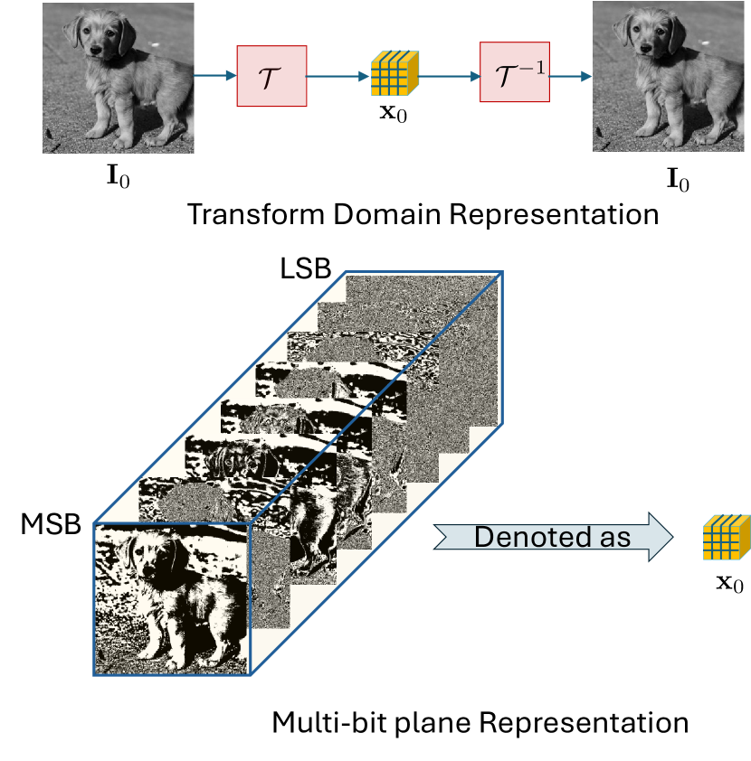
Figure 1: Multi-bit plane representation of images. An image $\mathbf{I}_{0}$ is represented by ${\bf x}_{0}$ through a bijective transform $\mathcal{T}$. In this work, $\mathcal{T}$ decomposes the input image into bitplanes, organized within the tensor ${\bf x}_{0}$, where MSB planes capture the most significant bits and LSB planes capture the least significant bits. Notably, these representations are binary, satisfying $\mathbf{I}_{0}=\sum_{k=0}^{n-1}{\bf x}_{0}(k)2^{k}$ for a gray-scale image or RGB competent of a color image. The MSB planes exhibit high pixel correlation, while the LSB planes display greater independence across pixels.

3.2 Binary Diffusion Probabilistic Model

BDPM shown in Figure 2 is a novel approach for generative modeling that leverages the simplicity of binary data representations. This method involves adding noise through XOR operation, which makes it particularly well-suited for handling binary data. Below, we describe the key aspects of the BDPM methodology in detail.

In BDPM noise is added to the data by flipping bits using the XOR operation as defined by the mapper $\mathcal{M}_{t}$ at each step $t$. The amount of noise added is quantified by the proportion of bits flipped. Let ${\bf x}_{0}(k)\in\{0,1\}^{h\times w}$ with $k=0,...,n-1$ for each color competent of the color image be the original binary bit-plane of dimension $h\times w$, and ${\bf z}_{t}(k)\in\{0,1\}^{h\times w}$ be a random binary noise plane at time step $t$. The noisy bit plane ${\bf x}_{t}(k)$ at the output of $\mathcal{M}_{t}$ is obtained as: ${\bf x}_{t}(k)={\bf x}_{0}(k)\oplus{\bf z}_{t}(k)$ , where $\oplus$ denotes the XOR operation. The noise level is defined as the fraction of bits flipped in ${\bf z}_{t}(k)$ in the mapper $\mathcal{M}_{t}$ at step $t$, with the number of bits flipped ranging within the probability range $[0,0.5]$ as a function of the timestep and potentially as a function of $k$.

The denoising network $\bm{g}_{\theta}^{B}({\bf x}_{t},t,{\bf y}_{e})$ is trained to predict both the added noise tensor of bit planes ${\bf z}_{t}$ and the clean tensor of image bit planes ${\bf x}_{0}$ from the noisy tensor ${\bf x}_{t}$. We employ binary cross-entropy (BCE) loss for each bit plane to train the denoising network. The loss function is averaged over the batch of $M$ samples:

where $\theta$ represents the parameters of the denoising network, ${\bf x}_{0}^{(m)}$ and $\hat{{\bf x}}_{0}^{(m)}$ are the $m$-th samples of the true clean tensors and the predicted clean tensors, respectively. Similarly, ${\bf z}_{t}^{(m)}$ and $\hat{{\bf z}}_{t}^{(m)}$ are the $m$-th samples of the true added noise tensors and the predicted noise tensors, respectively. ${\bf y}_{e}=\mathcal{E}_{y}({\bf I}_{y})$ denotes the encoded conditional image ${\bf I}_{y}$ that can represent the low-resolution down-sampled image, blurred image or image with removed parts that should be in-painted. The losses $\mathcal{L}_{x}$ and $\mathcal{L}_{z}$ denote BCE losses computed for each bit plane $k$ and the pixel coordinates $i\in\{1,\cdots,h\}$ and $j\in\{1,\cdots,w\}$ withing each bit plane.

In order to balance bit-planes during training of the denoiser network, we apply linear bit-plane weighting, where the weight for MSB is set to 1, weight for LSB is set to 0.1 and for others weights are linearly interpolated between 1 and 0.1. This fine-grained weighting can not be achieved with the MSE loss in a tractable form.

The output of the denoiser $\bm{g}_{\theta}^{B}({\bf x}_{t},t,{\bf y}_{e})$ is binarized via a mapper $\mathcal{Q}$ prior to applying the inverse transform ${\mathcal{T}}^{-1}$ as shown in Figure 2.

When sampling (Figure 2 right), we start from a random binary tensor ${\bf x}_{t}$ at timestep $t=T$, along with the conditioning state ${\bf I}_{y}$, encoded into ${\bf y}_{e}$. For each selected timestep in the sequence $\{T,\ldots,0\}$, denoising is applied to the tensor. The denoised tensor $\hat{{\bf x}}_{0}$ and the estimated binary noise $\hat{{\bf z}}_{t}$ are predicted by the denoising network. These predictions are then processed using a sigmoid function and binarized with a threshold in the mapper $\mathcal{Q}$. During sampling, we use the denoised tensor $\hat{{\bf x}}_{0}$ directly. Then, random noise ${\bf z}_{t}$ is generated and added to $\hat{{\bf x}}_{0}$ via the XOR operation: ${\bf x}_{t}=\hat{{\bf x}}_{0}\oplus{\bf z}_{t}$. The sampling algorithm is summarized in Algorithm 1.

Algorithm 1 Sampling algorithm.

1:${\bf x}_{t}\leftarrow$ random binary tensor

2:${\bf I}_{y}\leftarrow$ condition/label

3:${\bf y}_{e}\leftarrow\mathcal{E}_{y}({\bf I}_{y})$ apply condition encoding

4:$threshold\leftarrow$ threshold value to binarize $\triangleright$ Default 0.5

5:$\bm{g}_{\theta}^{B}({\bf x}_{t},t,{\bf y}_{e})\leftarrow$ pre-trained denoiser network

6:for $t\in\{T,\dots,0\}$ do $\triangleright$ Selected timesteps

7:  $\hat{{\bf x}}_{0},\hat{{\bf z}}_{t}\leftarrow\bm{g}_{\theta}^{B}({\bf x}_{t},t,{\bf y}_{e})$

8:  $\hat{{\bf x}}_{0}\leftarrow\sigma(\hat{{\bf x}}_{0})>threshold$ $\triangleright$ $\mathcal{Q}$: Apply sigmoid and compare to threshold

9:  ${\bf z}_{t}\leftarrow get\_binary\_noise(t)$ $\triangleright$ Generate random noise

10:  ${\bf x}_{t}\leftarrow\hat{{\bf x}}_{0}\oplus{\bf z}_{t}$ $\triangleright$ Update ${\bf x}_{t}$ using XOR with ${\bf z}_{t}$

11:end for

12:return ${\mathcal{T}}({\bf x}_{t})^{-1}$

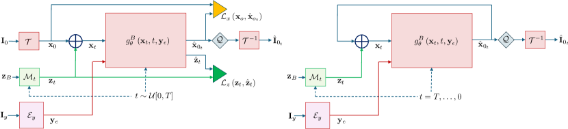
Figure 2: Binary Diffusion training (left) and sampling (right) schemes.

4 Experimental results

We evaluate the proposed method on the following tasks: 4× super-resolution task that scales images from $64\times 64$ to $256\times 256$ pixels using the FFHQ [19] and CelebA [27] datasets, medium size mask inpainting using FFHQ of the size $512\times 512$ pixels, CelebA of the size $256\times 256$ pixels, CelebA-HQ [18] of the size $512\times 512$ and blind image restoration on CelebA of the size $256\times 256$.

In all experiments, we use the same U-Net denoising model with 35.8M parameters, with 4 convolution downsampling blocks, self-attention[40] in the bottom downsampling block, and linear attention[20] in other downsampling blocks.

4.1 Datasets

We perform experiments on three datasets: CelebA [27], FFHQ [19], and CelebA-HQ[18]. CelebA contains 202,599 celebrity images at a resolution of approximatelly $178\times 218$ pixels, each annotated with 40 facial attributes, we use train split for training and test split for evaluation. FFHQ consists of 70,000 high-quality face images at $1024\times 1024$ resolution, offering diverse variations in age, ethnicity, and background. For all experiments, we split FFHQ into 60,000 images for training and 10,000 for evaluation. CelebA-HQ is a high-quality version of CelebA, comprising 30,000 images at $1024\times 1024$ resolution. For the super-resolution task, we utilize CelebA and FFHQ datasets. The inpainting task employs all three datasets: CelebA, FFHQ, and CelebA-HQ. For blind image restoration, our model is pretrained on FFHQ and evaluated on CelebA.

4.2 Metrics

We evaluate the model performance using Fréchet Inception Distance (FID) [13], Learned Perceptual Image Patch Similarity (LPIPS) [53], Peak Signal-to-Noise Ratio (PSNR), Structural Similarity Index Measure (SSIM) [45], and the number of function evaluations (NFEs), which corresponds to the number of model executions on the studied downstream tasks. Perceptual Image Defect Similarity (P-IDS), Unweighted Image Defect Similarity (U-IDS) [54] are also added to inpaiting evaluation.

4.3 Super-resolution

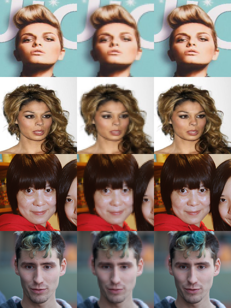
Figure 3: Super-resolution samples. First column: ground truth high-resolution samples, second column: low-resolution 4 times down-sampled samples, third column: samples reconstructed by BDPM model. First and second rows are from CelebA dataset, third and forth rows are from FFHQ dataset.

The super-resolution process downscales the original $256\times 256$ images by selecting every fourth pixel, then upsamples them back to $256\times 256$ using bilinear interpolation. This upsampled image serves as the conditioning ${\bf I}_{y}$ (see Figure 2). The images are transformed into bitplanes via $\mathcal{T}$ and concatenated with the input channels for the denoiser network. For super-resolution, we fix the diffusion steps at 30. Examples of ground truth, low-resolution inputs, and BDPM-upsampled images appear in Figure 3, with more examples and per-pixel variance shown in the Supplementary Materials.

BDPM model is compared against SOTA GAN-based: HiFaceGAN [48] and diffusion-based methods: DPS [6], DDRM [21], and DiffPIR [58] on FFHQ dataset. On the FFHQ dataset, results are sumarized in Table 1, BDPM achieves superior results in LPIPS, PSNR, and SSIM metrics compared to previous approaches. On CelebA BDPM is compared against SOTA GAN-based models: PULSE [30], diffusion-based models: ILVR [5], DDNM [44], DiffFace [22], ResShift [51], DiT-SR [4] and transformer-based models: VQFR [11], CodeFormer [56], results are sumarized in Table 2, BDPM outperforms other methods in FID, LPIPS, and PSNR metrics.

Method	FID	LPIPS	PSNR	SSIM	NFEs
HiFaceGAN [48]	5.36	-	28.65	0.816	1
DPS [6]	39.35	0.214	25.67	0.852	1000
DDRM [21]	62.15	0.294	25.36	0.835	1000
DiffPIR [58]	58.02	0.187	29.17	-	20
DiffPIR	47.8	0.174	29.52	-	100
BDPM (our)	5.71	0.151	30.05	0.864	30

Table 1: Comparsion of super-resolution approaches on FFHQ dataset. The best metrics are shown in bold and second best underscored.

Method	FID	LPIPS	PSNR	SSIM	NFEs
PULSE [30]	40.33	-	22.74	0.623	100
DDRM [21]	31.04	-	31.04	0.941	100
ILVR [5]	29.82	-	31.59	0.943	100
VQFR [11]	25.24	0.411	-	-	1
CodeFormer [56]	26.16	0.324	-	-	1
DiffFace [22]	23.21	0.338	-	-	100
DDNM [44]	22.27	-	31.63	0.945	100
ResShift [51]	17.56	0.309	-	-	4
DiT-SR [4]	19.65	0.337	-	-	4
BDPM (our)	3.5	0.116	32.01	0.91	30

Table 2: Comparsion of super-resolution approaches CelebA dataset. The best metrics are shown in bold and second best underscored. If the evaluation metric is not available in the paper, or in available public benchmark, it is marked as ‘-‘.

4.4 Inpainting

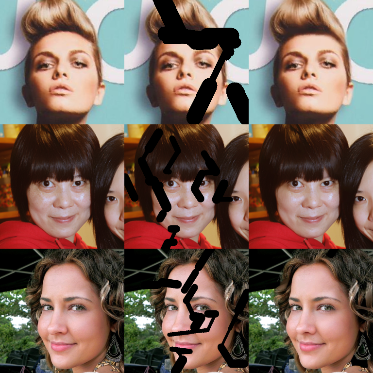
Figure 4: Inpainting samples. First column: ground truth high-resolution sample, second row: masked sample, third row: inpainted by BDPM model. First row: CelebA dataset, second row: FFHQ dataset, third row: CelebA dataset.

The inpainting problem involves reconstructing missing (masked) regions in images.

In our approach, we use medium size masks, that mask between 10% and 30% of the total image size. In our approach, the masked image ${\bf I}_{m}$ is transformed into bitplanes, and the missing pixels are replaced with random binary values $\{0,1\}$. The mask is also provided to the denoiser network, and both the masked image and the mask are concatenated along the channel dimension as input to the model, e.g., ${\bf I}_{y}=[{\bf M},{\bf I}_{m}]$, where ${\bf M}$ is inpainting mask and ${\bf I}_{m}$ is masked image. For the inpatining task, we fix the number of diffusion steps to 100. Examples of ground truth, masked images and inpainted by BDPM images are shown in Figure 4. More examples of inpainted images are presented in Supplementary material.

We compare BDPM against the state-of-the-art methods: LaMa [39], CoModGAN [54], TFill [55], and SH-GAN [47] on FFHQ, results are summarized in Table 3, BDPM outperforms consifered methods on FID, PSNR, SSIM, P-IDS and U-IDS metrics.

On the CelebA dataset, BDPM is compared against SOTA GAN-based methods: RePaint [29], EdgeConnect [31], DeepFillV2 [49], LaMa [39], diffusion-based methods: DDRM [21], DDNM [44] and transformer-based methods: ICT [41], MAT [25], results are sumarized in Table 4, BDPM achieves superior results on perceptual metrics such as FID, P-IDS, and U-IDS.

For the CelebA-HQ dataset, we use the model pretrained on FFHQ and evaluate it on 10,000 randomly selected images. BDPM is compared against SOTA GAN-based methods: EdgeConnect [31], DeepFillv2 [49], AOT GAN [52], MADF [57], LaMa [39], CoModGAN [54] and transformer-based methods: ICT [39], MAT [25], results are sumarized in Table 5, BDPM surpasses current SOTA on perceptual metrics FID and LPIPS.

Method	FID	LPIPS	PSNR	SSIM	P-IDS	U-IDS	NFEs
LaMa [39]	19.6	0.287	18.99	0.7178	-	-	1
CoModGAN [54]	3.7	0.247	18.46	0.6956	16.6	29.4	1
TFill [55]	3.5	0.053	-	-	-	-	1
SH-GAN [47]	3.4	0.245	18.43	0.6936	-	-	1
BDPM (our)	1.3	0.059	28.7	0.961	17.43	33.07	100

Table 3: Comparison of inpainting approaches FFHQ dataset. The best metrics are shown in bold and second best underscored. If the evaluation metric is not available in the paper, or in available public benchmark, it is marked as ‘-‘.

Method	FID	LPIPS	PSNR	SSIM	P-IDS	U-IDS	NFEs
RePaint [29]	14.19	-	35.2	0.981	-	-	2500
DDRM [21]	12.53	-	34.79	0.982	-	-	100
EdgeConnect [31]	12.16	-	-	-	0.84	2.31	1
DeepFillV2 [49]	13.23	-	-	-	0.84	2.62	1
ICT [41]	10.92	-	-	-	0.9	5.23	1
LaMa [39]	8.75	-	-	-	2.34	8.77	1
MAT [25]	5.16	-	-	-	13.9	25.13	1
DDNM [44]	4.54	-	35.64	0.982	-	-	100
BDPM (our)	1.96	0.08	28.3	0.928	15.04	27.01	100

Table 4: Comparsion of inpainting approaches CelebA dataset. The best metrics are shown in bold and second best underscored. If the evaluation metric is not available in the paper, or in available public benchmark, it is marked as ‘-‘.

Method	FID	LPIPS	PSNR	SSIM	P-IDS	U-IDS	NFEs
EdgeConnect [31]	10.58	0.101	-	-	4.14	12.45	1
DeepFillv2 [49]	10.11	0.117	-	-	3.11	9.52	1
AOT GAN [52]	4.65	0.074	-	-	7.92	20.45	1
MADF [57]	3.39	0.068	-	-	12.06	24.61	1
ICT [41]	6.28	0.105	-	-	2.24	9.99	1
LaMa [39]	4.05	0.075	-	-	9.72	21.57	1
CoModGAN [54]	3.26	0.073	-	-	19.95	31.41	1
MAT [25]	2.86	0.065	-	-	21.15	32.56	1
BDPM (our)	1.17	0.06	29.41	0.925	14.14	28.4	100

Table 5: Comparsion of inpainting approaches CelebA-HQ dataset. The best metrics are shown in bold and second best underscored. If the evaluation metric is not available in the paper, or in available public benchmark, it is marked as ‘-‘.

4.5 Blind image restoration

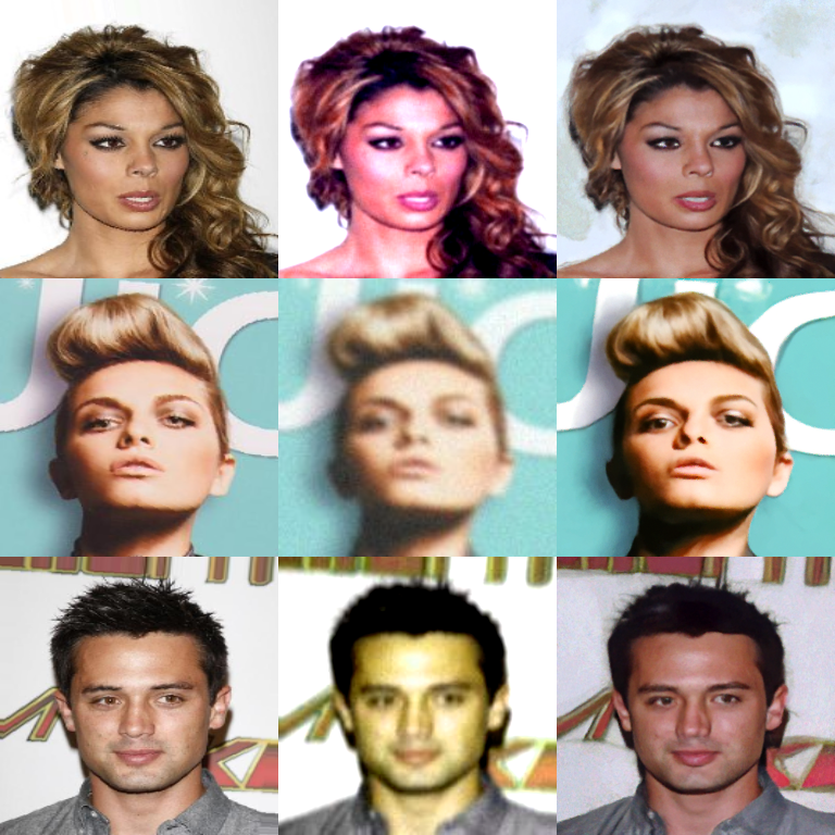
Figure 5: Blind image restoration samples from CelebA dataset. First column: ground truth high-resolution sample, second row: degraded sample, third row: restored by BDPM model.

Blind image restoration aims to recover high-quality images from degraded inputs without knowing the specific degradation. This task is challenging due to varied degradations. To address this, we pretrain our BDPM model on a synthetic blind image restoration dataset from FFHQ images at $256\times 256$ resolution, applying random combinations of perturbations. Details on these perturbations and parameters are in the Supplementary Materials, with examples of ground truth, perturbed, and restored images shown in Figure 5.

In our experiments, we fix the number of sampling steps for BDPM to 40. The BDPM model is compared against the state-of-the-art methods including CodeFormer [56], DR2 [46], BFRFormer [10], DiffBIR [26], GFP-GAN [43], BFRfusion [3], StableSR [42], and DifFace [50], results are sumarized in Table 6, BDPM achieves superior performance on metrics such as FID and SSIM.

Method	FID	LPIPS	PSNR	SSIM	NFEs
CodeFormer [56]	60.62	0.299	22.18	0.61	1
DR2 [46]	58.94	0.3979	24.44	0.6784	250
BFRFormer [10]	57.37	0.27	22.83	-	1
DiffBIR [26]	47.9	0.3786	25.6	0.6809	50
GFP-GAN [43]	42.62	0.3646	25.08	0.6777	1
BFRffusion [3]	40.74	0.3621	26.2	0.6926	50
StableSR [42]	39.73	0.3637	24.84	0.6772	200
DifFace [50]	20.29	0.461	23.44	0.67	100
BDPM (our)	12.93	0.293	24.58	0.7415	40

Table 6: Comparison of Bling Image Restoration on CelebA dataset. The best metrics are shown in bold and second best underscored. If the evaluation metric is not available in the paper, or in available public benchmark, it is marked as ‘-‘.

4.6 Comparison with Posterior Sampling Methods

BDPM is compared to posterior sampling models such as DPS [6], DDRM [21], DiffPIR [58], DDNM [44], DiffBIR [26], BFRFusion [3], and StableSR [42] (see Tables 1, 2, 3, and 6). These methods leverage large pretrained diffusion models [8, 33] and adapt them for specific tasks using posterior sampling. Details on number of parameters for each model are provided in Supplementary Materials. Although these methods do not require additional training, they often need more sampling steps and rely on larger models for inference, making them less suitable for large-scale deployment. In contrast, the proposed method requires training but is compact with 35.8 million parameters and enables fast sampling. It outperforms posterior sampling methods, making it more suitable for large-scale applications.

4.7 Comparison with Gaussian Diffusion

To compare BDPM with the classical Gaussian DDPM model, we pre-trained both models for conditional image generation on the CIFAR-10 [24] dataset, using identical architectures except that BDPM accepts 24 input channels (3 color channels split into 8 bitplanes each). Both models were pre-trained for 200,000 iterations with a batch size of 256, the Adam optimizer [23], a constant learning rate of $10^{-4}$, and EMA updates every 10 steps with a decay rate of $\beta=0.995$. Classifier-free guidance [14] was applied before binarization, with guidance scales of 3 for DDPM/DDIM [38] and 5 for BDPM. We generated 50,000 samples per model for each number of sampling steps. Figure 6 shows the relationship between sampling steps and FID for each model.

For a fair comparison, we evaluated BDPM against baseline DDPM and DDIM sampling methods. While future work will adapt samplers specifically for BDPM, this study focuses on comparing sampling trends across DDPM, DDIM, and BDPM.

Our results show that BDPM performs competitively with DDPM and DDIM in conditional image generation on the CIFAR-10 dataset, achieving convergence with fewer sampling steps under identical architectures and training conditions. Additional analysis is available in the Supplementary Materials.

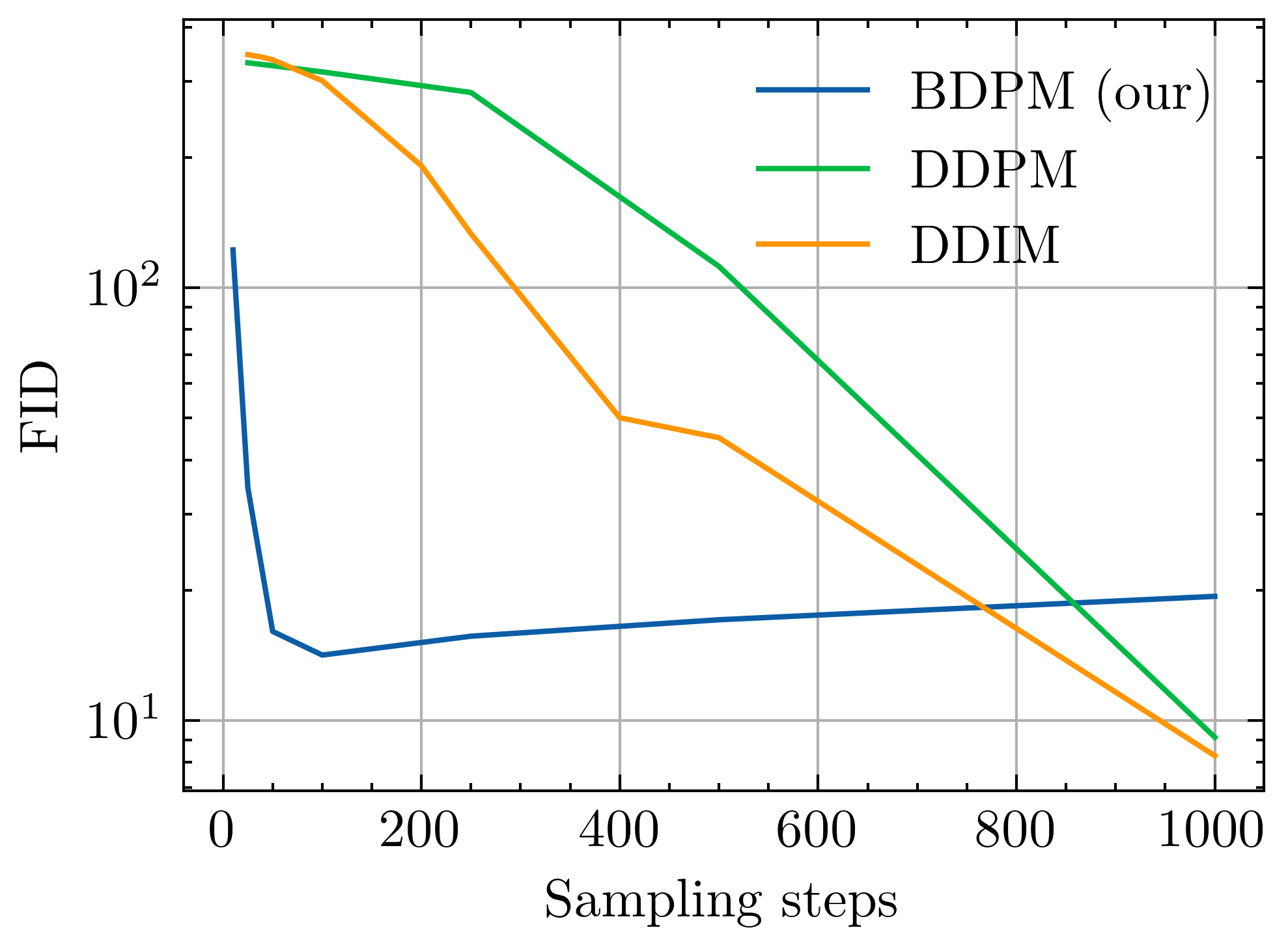
Figure 6: Relationship between the FID metric and the number of sampling steps for conditional image generation on the CIFAR-10 dataset. As shown, BDPM’s FID saturates beyond a certain point, indicating no further improvement with additional sampling steps. While DDPM and DDIM achieve better results when sampling for 1,000 steps, BDPM exhibits a distinctive trend worth noticing, where bigger number of sampling steps do not lead to better generation in terms of FID.

5 Conclusions

In this work, we introduce the BDPM, a novel diffusion-based generative framework tailored for binary data representations. Unlike traditional DDPMs, which rely on continuous representations and Gaussian noise, BDPM utilizes a binary bit-plane approach with XOR-based noise transformations and binary cross-entropy loss. The model is specifically optimized for binary data, leading to improved efficiency and effectiveness across image restoration tasks.

Our experiments show that BDPM achieves state-of-the-art performance in super-resolution, inpainting, and blind image restoration on datasets like FFHQ, CelebA, and CelebA-HQ. BDPM requires fewer inference steps than Gaussian-based models, underscoring its computational efficiency.

By using binary cross-entropy instead of traditional MSE loss, BDPM aligns better with the discrete nature of digital images, enhancing convergence and preserving binary data integrity for faster, stable training. BDPM’s compact size of 35.8M parameters also makes it well-suited for real-world applications with limited computational resources.

Supplementary Material

6 Ablation studies

We perform the ablation study on the loss function. We pretrain 3 identical BDPMs for conditional image generation task on the CIFAR-10 [24] dataset with different losses: loss on added noise estimation $\mathcal{L}_{z}(\hat{{\bf z}}_{t}^{(m)},{\bf z}_{t}^{(m)})$, loss on image estimation $\mathcal{L}_{x}(\hat{{\bf x}}_{0}^{(m)},{\bf x}_{0}^{(m)})$ and loss on both noise and image estimations $\mathcal{L}_{x}(\hat{{\bf x}}_{0}^{(m)},{\bf x}_{0}^{(m)})+\mathcal{L}_{z}(\hat{{\bf z}}_{t}^{(m)},{\bf z}_{t}^{(m)})$. Models were pre-trained for 200,000 iterations with a batch size of 256, using the Adam optimizer [23], a constant learning rate of $10^{-4}$, and exponential moving average (EMA) updates every 10 steps with a decay rate of $\beta=0.995$. During pre-training and sampling, we employed classifier-free guidance [14], applied before the binarization step. Then we sample 50000 images for each model, using 50 sampling steps and guidance 5. Models are evaluated using FID metric. Results are summarized in Table 7. The best FID is achieved when using combination of two losses for the image and added noise estimation.

Loss	FID
$\mathcal{L}_{z}(\hat{{\bf z}}_{t}^{(m)},{\bf z}_{t}^{(m)})$	17.88
$\mathcal{L}_{x}(\hat{{\bf x}}_{0}^{(m)},{\bf x}_{0}^{(m)})$	19.91
$\mathcal{L}_{x}(\hat{{\bf x}}_{0}^{(m)},{\bf x}_{0}^{(m)})+\mathcal{L}_{z}(\hat{{\bf z}}_{t}^{(m)},{\bf z}_{t}^{(m)})$	13.85

Table 7: Loss function ablation study.

7 Implementation details

Denoiser architecture and training parameters: We use PyTorch [1] and Accelerate [12] deep learning frameworks for both training and inference of the model. The U-Net denoiser network [34] is inspired by the denoiser from [8]. The U-Net denoiser consists of four convolutional downsampling blocks. The bottom downsampling block uses self-attention [40], while linear attention [20] is used in all layers except the last one. To accelerate training and inference, we incorporate FlashAttention [7] and bfloat16 precision. Our denoiser consists of 35.8 million parameters. Sinusoidal timestep conditioning [15] is integrated as biases in every block. Image conditioning (for tasks such as super-resolution, inpainting, and restoration) is appended as extra channels to the input. Vector conditioning (e.g., one-hot encoded classes) is added as biases to every layer. We use the same training setup across all tasks. Specifically, we use EMA distillation for the denoiser model, and the EMA model is then used for evaluation purposes. During training, the denoiser predicts both the clean image’s bitplanes and the binary noise associated with each bitplane. At each timestep $t\in[0,T]$, the amount of noise added to each bitplane remains constant. However, since different bitplanes hold varying levels of importance, we adopt a linearly interpolated weighting scheme for the binary cross-entropy loss. The most significant bitplane is assigned a weight of $1$, while the least significant bitplane receives a weight of $0.1$, with intermediate bitplanes assigned weights that are linearly interpolated between these values. This approach ensures that higher bitplanes, which contribute more to the image’s overall structure and quality, are prioritized during training. The weights for noise prediction are kept constant at $1$ for each bitplane. We define the noise level as the fraction of bits flipped in $\bm{z}_{t}(k)$ by the mapper $\mathcal{M}_{t}$ at step $t$, with the number of bits flipped ranging within the probability range $[0,0.5]$ as a function of the timestep $t$ and potentially as a function of $k$.

To control this noise level, we use quadratic noise scheduling for the diffusion process. The noise schedule $\beta_{t}$ at time step $t$ determines the probability of bits being flipped and is defined as:

$$\beta_{t}=\left(\sqrt{\beta_{\text{start}}}+\frac{t}{T}\left(\sqrt{\beta_{\text{end}}}-\sqrt{\beta_{\text{start}}}\right)\right)^{2},$$ (3)

where $T$ is the total number of time steps (default is $1000$), $\beta_{\text{start}}$ is the minimum value of the noise, $10^{-5}$ by default, $\beta_{\text{start}}$ is maximum value of the noise. $\beta_{t}$ controls the probability of the bit to be flipped.

The training parameters are summarized in Table 8.

Hyperparameter	Value
Optimizer	AdamW
Learning rate	$1\times 10^{-4}$
Weight decay	$1\times 10^{-6}$
Number of training steps	500,000
Gradient accumulation	No
EMA update frequency	10 steps
EMA decay	0.995
Noise schedule	Quadratic
Number of diffusion steps	1,000
Image bitplane weights	Linear
Mask bitplane weights	Constant
Precision	bfloat16
Batch size	64 for $256\times 256$ images 8 for $512\times 512$ images

Table 8: Training Hyperparameters

Super-Resolution Implementation: The conditioning is performed by concatenating the bitplanes of the bilinearly upsampled low-resolution image as extra channels. During training, we apply random cropping (ranging from 80% to 100% of the image height and width) and horizontal flipping as data augmentation techniques. For evaluation, we use the PSNR, SSIM, LPIPS, and FID metrics.

Inpainting Implementation: The conditioning is performed by concatenating the bitplanes of masked images, where masked pixels are replaced with random noise. Additionally, the mask is concatenated to the input. During training, we apply random cropping (ranging from 80% to 100% of the image height and width) and horizontal flipping as data augmentation techniques. For evaluation, we use the PSNR, SSIM, LPIPS, FID, P-IDS, and U-IDS metrics.

Blind Image Restoration Implementation: The conditioning is performed by concatenating the bitplanes of the perturbed image as extra channels. We pretrain our BDPM model on a synthetic blind image restoration dataset constructed from FFHQ images at a resolution of $256\times 256$. The degradations are simulated by randomly applying a combination of perturbations to the images, summarized in Table 9.

Perturbation	Parameters	Probability
Gaussian Blur	Kernel size: $21\times 21$ Kernel: isotropic or anisotropic $\sigma_{x},\sigma_{y}\in[0.1,7]$ Rotation angle $\in[-\pi,\pi]$	Always
Downsampling	Scale $[1,4]$	Always
Additive Gaussian Noise	Standard deviation $[0,15]/255$	Always
JPEG Compression	Quality factor $[50,100]$	Always
Color Shift	Shift per color $[-20/255,20/255]$	30%
Color Jitter	Brightness $[0.5,1.5]$ Contrast $[0.5,1.5]$ Saturation $[0,1.5]$ Hue $[-0.1,0.1]$	30%
Grayscale Conversion	—	1%

Table 9: Perturbations, Parameters, and Probabilities Used in the Degradation Process.

8 Number of parameters

The experimental part of the main section used several state-of-the-art Gaussian DDPM. Table 10 summarizes the number of parameters in these models.

Model	Parameters
DDPM [21]	554 M
DPS [6]	554 M
DiffPIR [58]	554 M
DDNM [44]	554 M
DiffBIR [26]	17.2 B
BFRffusion [3]	1.23 B
StableSR [42]	1.20 B
HiFaceGAN [48]	54 M
PULSE [30]	26.2 M
ILVR [5]	554 M
VQFR [11]	76.3 M
CodeFormer [56]	74 M
ResShift [51]	118.6 M
DiT-SR [4]	100.6 M
EdgeConnect [31]	27 M
DeepFillV2 [49]	4.1 M
AOT GAN [52]	15.2 M
MADF [57]	85M
ICT [39]	120 M
LaMa [39]	51 M
CoModGAN [54]	109 M
MAT [25]	62 M
TFill [55]	70 M
SH-GAN [47]	79.8 M
RePaint [29]	554 M
DR2 [46]	168 M
GFP-GAN [43]	56 M
DifFace [50]	176 M
BDPM (our)	35.8 M

Table 10: Number of parameters in compared models.

9 Effect of number of sampling steps

9.1 CIFAR10 generation

Figure 7 show the CIFAR10 samples, generated by the BDPM model for different number of sampling steps: ${1000,500,250,100,50,25}$. For every number of steps, we generate 10 samples for each class. We observe, that samples that are generated with larger number of sampling steps tend to be of better quality (less artifacts), but to be less diverse. For example, one can clearly see that for 1000 sampling steps in Figure 7 (a), for class airplane (first column), two samples (rows 3 and 8) look almost identical, the same can be observed for class track (last column), thress samples (rows 1, 3, 4) are almost identical. For smaller number of sampling steps, generated samples are more diverse, but they can be of lower quality (have most generated artifacts).

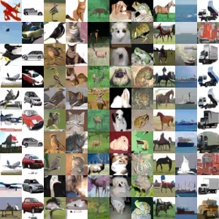
(a) 1000 sampling steps

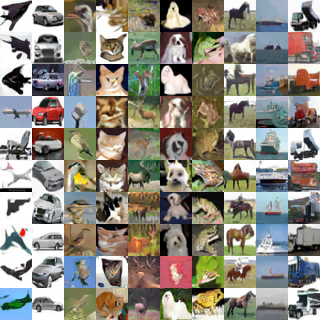
(b) 500 sampling steps

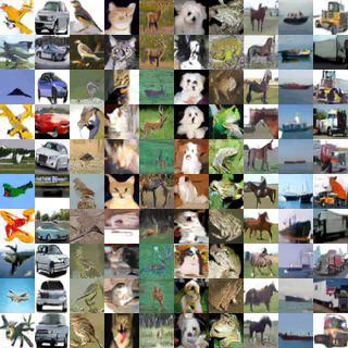
(c) 250 sampling steps

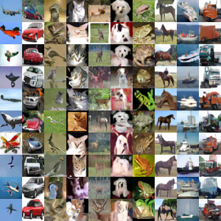
(d) 100 sampling steps

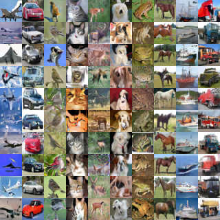
(e) 50 sampling steps

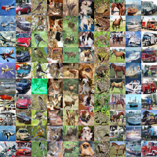
(f) 25 sampling steps

Figure 7: CIFAR10 conditional image generation with different number of sampling steps using BDPM model. Each column has samples of the same class.

9.2 Image-to-image translation

The similar trend, when BDPM with smaller number of steps achieves better results is shown with other generative tasks: super-resolution, inpainting and blind image restoration. For evaluation, we use the pretrained models on 256 $\times$ 256 FFHQ dataset. We show the relationship between number of sampling steps and evaluation metrics: FID, LPIPS, SSIM and PSNR. We evaluate model on 200 images for different number of sampling steps. The plots with relationship between the evaluation metrics and number of sampling steps are shows in the Figure 8. We select the optimal number of sampling steps, based on FID metric from evaluated 200 images for each of the tasks.

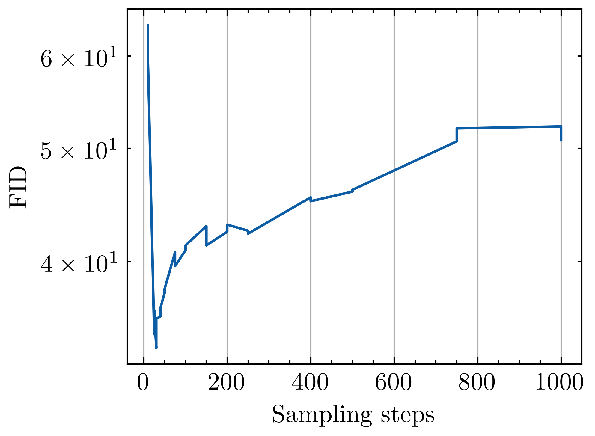
(a) FID

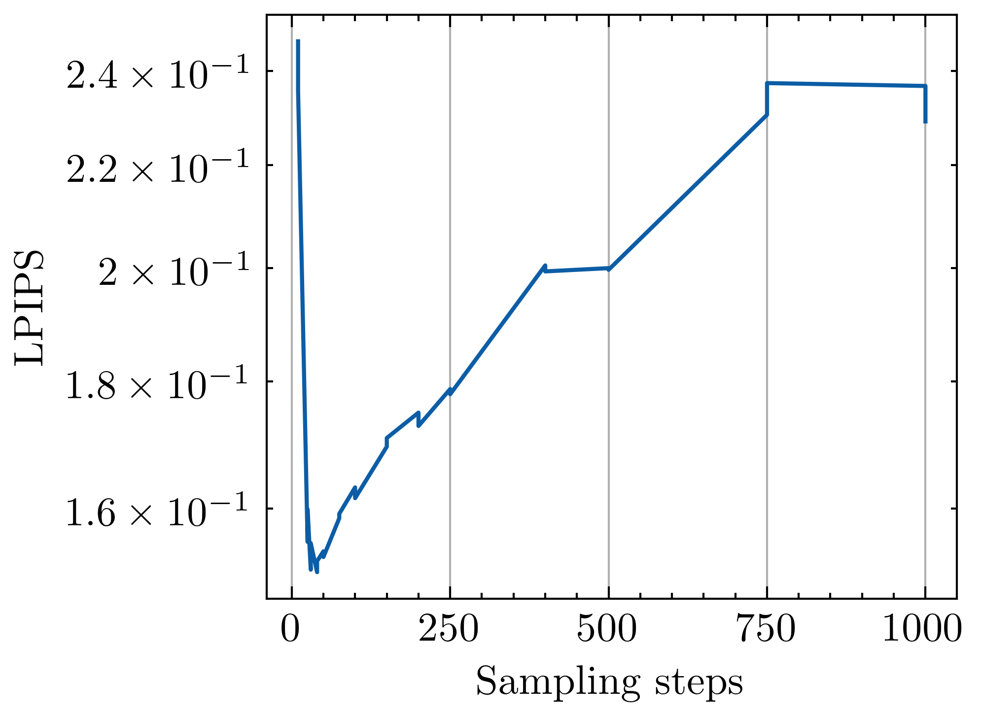
(b) LPIPS

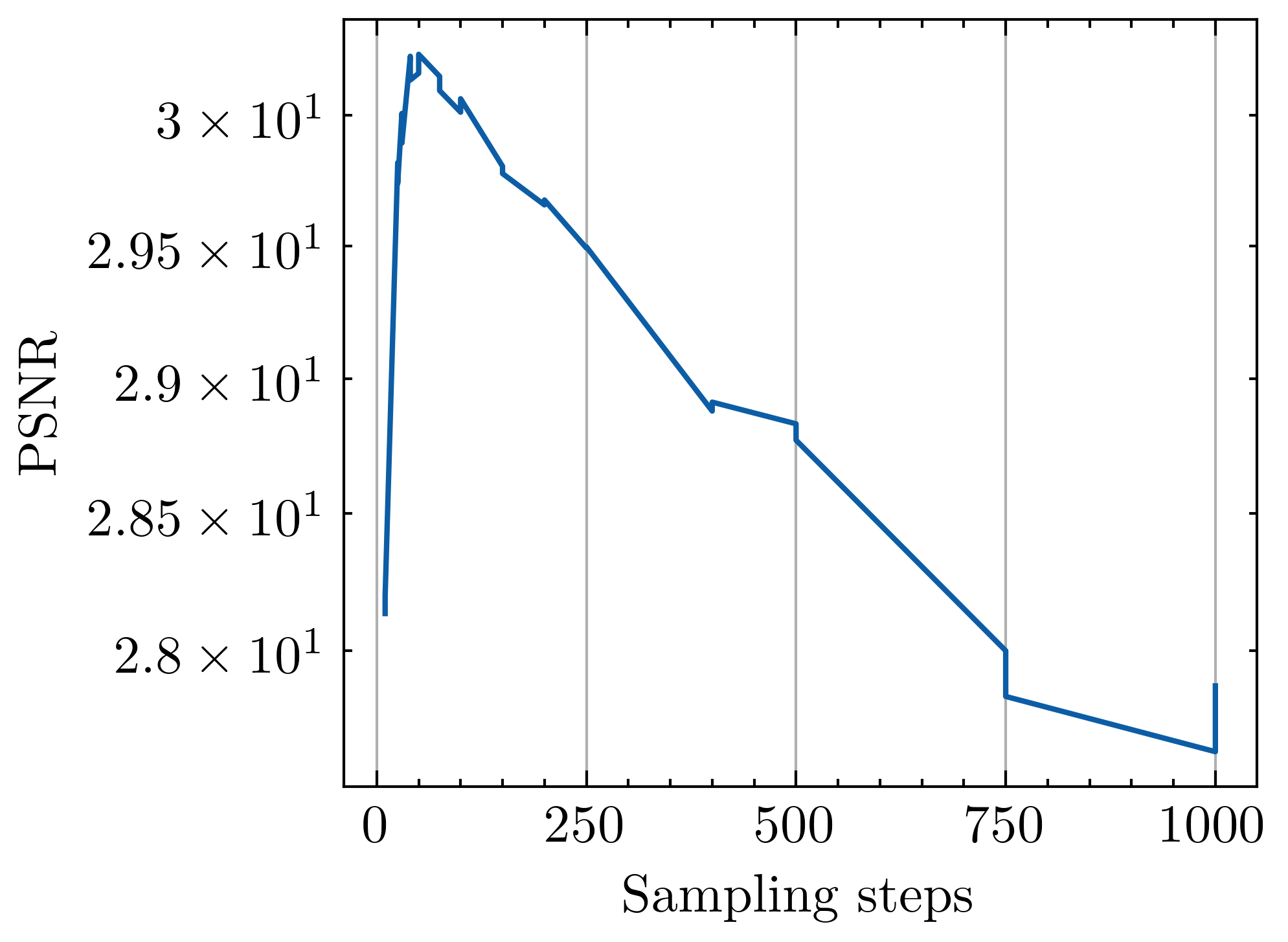
(c) PSNR

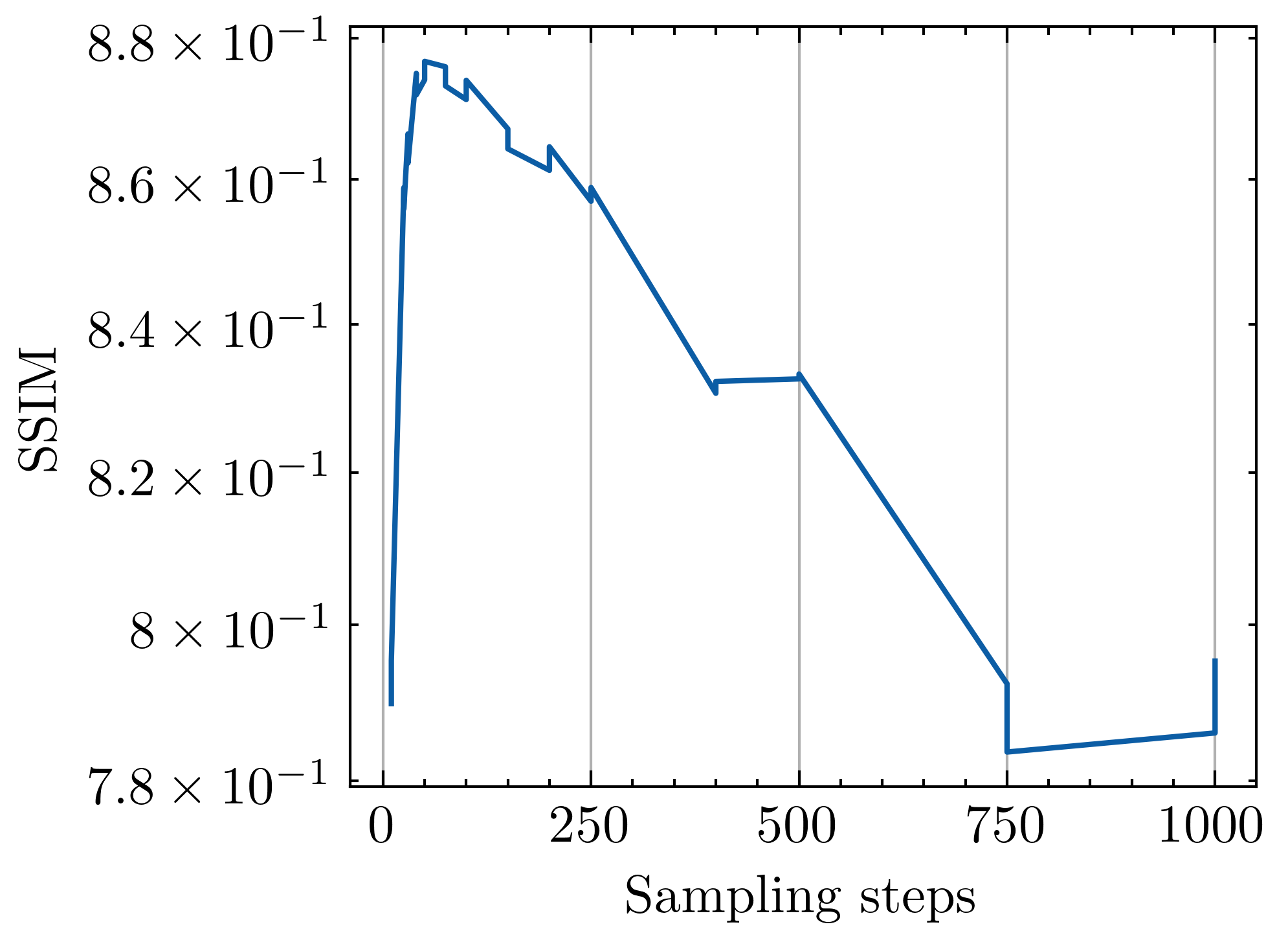
(d) SSIM

Figure 8: Relationship between the evaluation metrics and number of sampling steps on super-resolution task on FFHQ 256 $\times$ 256.

10 Results

Figures 9,10 show super-resolution samples generated using BDPM for datasets FFHQ and CelebA respectively. Ground truth images are shown in the first column, low resolution images are shown in the second columns, high-resolution image generated by BDPM, per-pixel variance over 10 high-resolution generations, per-pixel variances over 10 high-resolution generations are shown in the fourth columns.

Figures 11,12,13 show inpainting samples generated using BDPM for datasets FFHQ, CelebA and CelebA-HQ respectively. Masks are shown in the first row, ground truth images are shown in the first column, inpainting samples for each masks are shown in the columns 2 - 6.

Figure 14 shows blind image restortion results. Ground truth images are shown in the first column, perturbed images are shown in the second column, restored images are shown in columns 3 - 5.

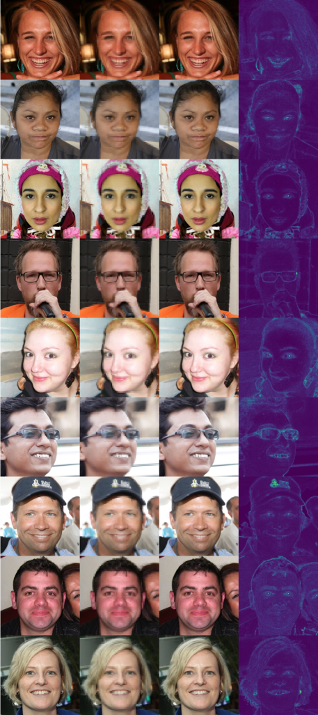
Figure 9: FFHQ superresolution 256 $\times$ 256. First column: ground truth image, second column: low resolution image, third column: high-resolution image generated by BDPM, forth column: per-pixel variance over 10 high-resolution generations.

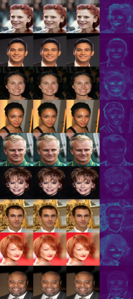
Figure 10: CelebA superresolution 256 $\times$ 256. First column: ground truth image, second column: low resolution image, third column: high-resolution image generated by BDPM, forth column: per-pixel variance over 10 high-resolution generations.

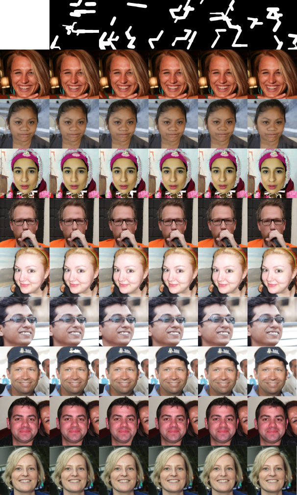
Figure 11: FFHQ inpainting 512 $\times$ 512. First row: inpainting masks, first column: ground truth images, 2-6 columns: inpainting images generated by BDPM.

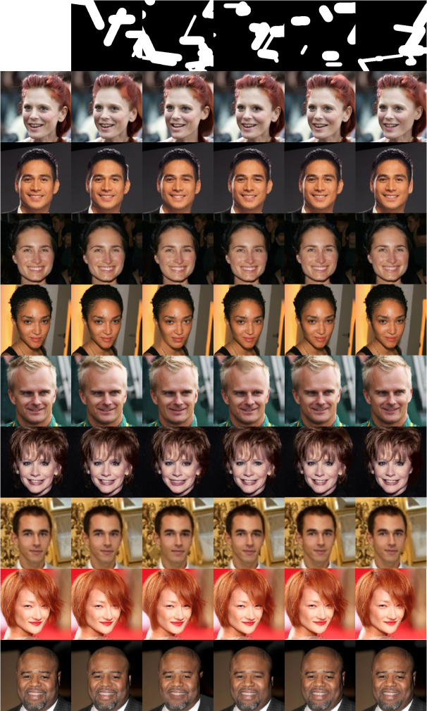
Figure 12: CelebA inpaint 256 $\times$ 256. First row: inpainting masks, first column: ground truth images, 2-6 columns: inpainting images generated by BDPM.

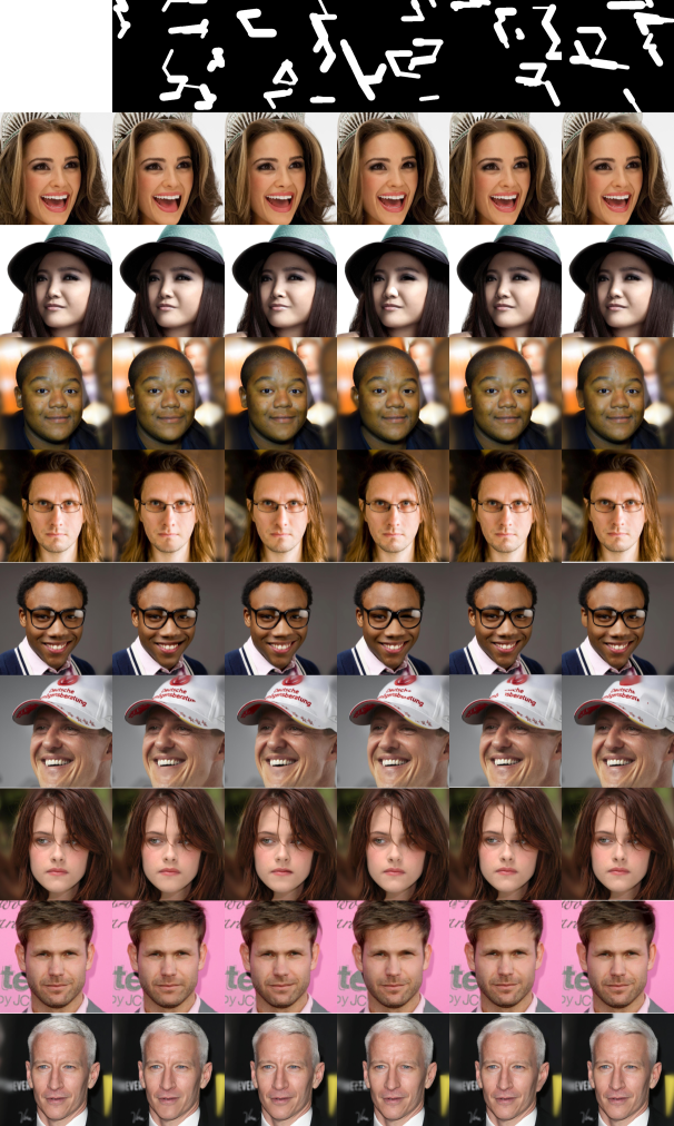
Figure 13: CelebA-HQ inpaint 512 $\times$ 512. First row: inpainting masks, first column: ground truth images, 2-6 columns: inpainting images generated by BDPM.

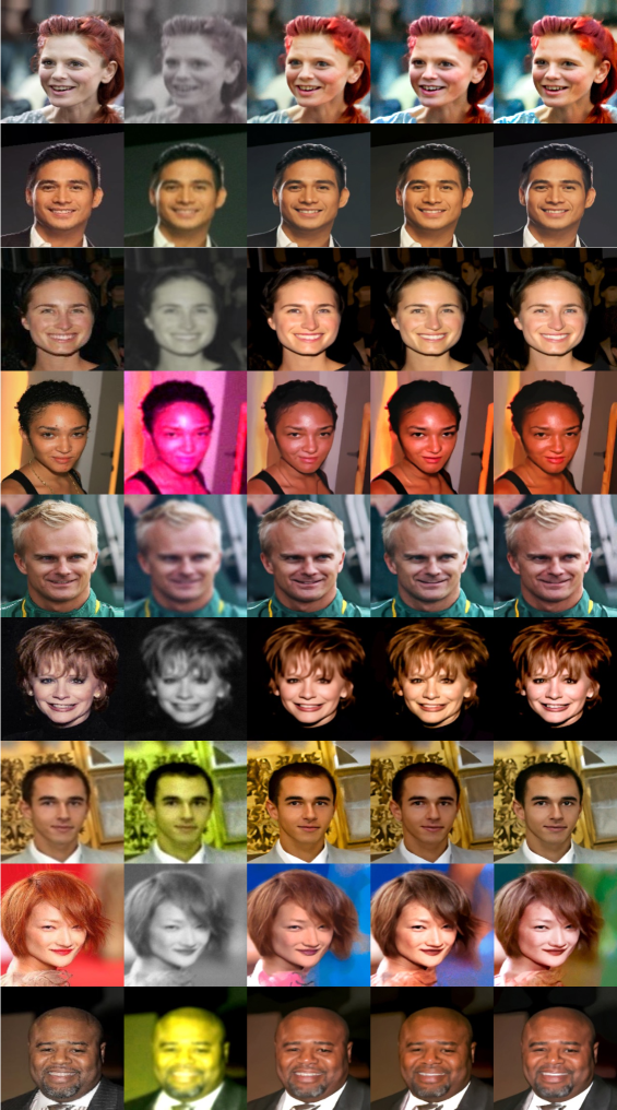
Figure 14: CelebA blind image restoration 256 $\times$ 256. First column: ground truth images, second column: distorted images, 3-5 columns: images restored by BDPM.

References

- Ansel et al. [2024] Jason Ansel, Edward Yang, Horace He, Natalia Gimelshein, Animesh Jain, Michael Voznesensky, Bin Bao, Peter Bell, David Berard, Evgeni Burovski, Geeta Chauhan, Anjali Chourdia, Will Constable, Alban Desmaison, Zachary DeVito, Elias Ellison, Will Feng, Jiong Gong, Michael Gschwind, Brian Hirsh, Sherlock Huang, Kshiteej Kalambarkar, Laurent Kirsch, Michael Lazos, Mario Lezcano, Yanbo Liang, Jason Liang, Yinghai Lu, CK Luk, Bert Maher, Yunjie Pan, Christian Puhrsch, Matthias Reso, Mark Saroufim, Marcos Yukio Siraichi, Helen Suk, Michael Suo, Phil Tillet, Eikan Wang, Xiaodong Wang, William Wen, Shunting Zhang, Xu Zhao, Keren Zhou, Richard Zou, Ajit Mathews, Gregory Chanan, Peng Wu, and Soumith Chintala. PyTorch 2: Faster Machine Learning Through Dynamic Python Bytecode Transformation and Graph Compilation. In 29th ACM International Conference on Architectural Support for Programming Languages and Operating Systems, Volume 2 (ASPLOS ’24). ACM, 2024.
- Austin et al. [2021] Jacob Austin, Daniel D Johnson, Jonathan Ho, Daniel Tarlow, and Rianne Van Den Berg. Structured denoising diffusion models in discrete state-spaces. Advances in Neural Information Processing Systems, 34:17981–17993, 2021.
- Chen et al. [2024] Xiaoxu Chen, Jingfan Tan, Tao Wang, Kaihao Zhang, Wenhan Luo, and Xiaochun Cao. Towards real-world blind face restoration with generative diffusion prior. IEEE Transactions on Circuits and Systems for Video Technology, 2024.
- Cheng et al. [2024] Kun Cheng, Lei Yu, Zhijun Tu, Xiao He, Liyu Chen, Yong Guo, Mingrui Zhu, Nannan Wang, Xinbo Gao, and Jie Hu. Effective diffusion transformer architecture for image super-resolution. arXiv preprint arXiv:2409.19589, 2024.
- Choi et al. [2021] Jooyoung Choi, Sungwon Kim, Yonghyun Jeong, Youngjune Gwon, and Sungroh Yoon. Ilvr: Conditioning method for denoising diffusion probabilistic models. in 2021 ieee. In CVF international conference on computer vision (ICCV), page 2, 2021.
- Chung et al. [2022] Hyungjin Chung, Jeongsol Kim, Michael T Mccann, Marc L Klasky, and Jong Chul Ye. Diffusion posterior sampling for general noisy inverse problems. arXiv preprint arXiv:2209.14687, 2022.
- Dao et al. [2022] Tri Dao, Dan Fu, Stefano Ermon, Atri Rudra, and Christopher Ré. Flashattention: Fast and memory-efficient exact attention with io-awareness. Advances in Neural Information Processing Systems, 35:16344–16359, 2022.
- Dhariwal and Nichol [2021] Prafulla Dhariwal and Alexander Nichol. Diffusion models beat gans on image synthesis. Advances in neural information processing systems, 34:8780–8794, 2021.
- Esser et al. [2021] Patrick Esser, Robin Rombach, and Björn Ommer. Taming transformers for high-resolution image synthesis. Proceedings of the IEEE/CVF Conference on Computer Vision and Pattern Recognition (CVPR), pages 12873–12883, 2021.
- Ge et al. [2024] Guojing Ge, Qi Song, Guibo Zhu, Yuting Zhang, Jinglu Chen, Miao Xin, Ming Tang, and Jinqiao Wang. Bfrformer: Transformer-based generator for real-world blind face restoration. In ICASSP 2024-2024 IEEE International Conference on Acoustics, Speech and Signal Processing (ICASSP), pages 3700–3704. IEEE, 2024.
- Gu et al. [2022] Yuchao Gu, Xintao Wang, Liangbin Xie, Chao Dong, Gen Li, Ying Shan, and Ming-Ming Cheng. Vqfr: Blind face restoration with vector-quantized dictionary and parallel decoder. In European Conference on Computer Vision, pages 126–143. Springer, 2022.
- Gugger et al. [2022] Sylvain Gugger, Lysandre Debut, Thomas Wolf, Philipp Schmid, Zachary Mueller, Sourab Mangrulkar, Marc Sun, and Benjamin Bossan. Accelerate: Training and inference at scale made simple, efficient and adaptable. https://github.com/huggingface/accelerate, 2022.
- Heusel et al. [2017] Martin Heusel, Hubert Ramsauer, Thomas Unterthiner, Bernhard Nessler, and Sepp Hochreiter. Gans trained by a two time-scale update rule converge to a local nash equilibrium. In Advances in Neural Information Processing Systems, 2017.
- Ho and Salimans [2022] Jonathan Ho and Tim Salimans. Classifier-free diffusion guidance. arXiv preprint arXiv:2207.12598, 2022.
- Ho et al. [2020] Jonathan Ho, Ajay Jain, and Pieter Abbeel. Denoising diffusion probabilistic models. Advances in neural information processing systems, 33:6840–6851, 2020.
- Ho et al. [2022] Jonathan Ho, William Chan, Chitwan Saharia, Jay Whang, Ruiqi Gao, Alexey Gritsenko, Diederik P Kingma, Ben Poole, Mohammad Norouzi, David J Fleet, et al. Imagen video: High definition video generation with diffusion models. arXiv preprint arXiv:2210.02303, 2022.
- Hoogeboom et al. [2021] Emiel Hoogeboom, Didrik Nielsen, Priyank Jaini, Patrick Forré, and Max Welling. Argmax flows and multinomial diffusion: Learning categorical distributions. Advances in Neural Information Processing Systems, 34:12454–12465, 2021.
- Karras [2017] Tero Karras. Progressive growing of gans for improved quality, stability, and variation. arXiv preprint arXiv:1710.10196, 2017.
- Karras et al. [2019] Tero Karras, Samuli Laine, and Timo Aila. A style-based generator architecture for generative adversarial networks. In Proceedings of the IEEE/CVF Conference on Computer Vision and Pattern Recognition, pages 4401–4410, 2019.
- Katharopoulos et al. [2020] Angelos Katharopoulos, Apoorv Vyas, Nikolaos Pappas, and François Fleuret. Transformers are rnns: Fast autoregressive transformers with linear attention. In Proceedings of the 37th International Conference on Machine Learning (ICML), pages 5156–5165, 2020.
- Kawar et al. [2022] Bahjat Kawar, Michael Elad, Stefano Ermon, and Jiaming Song. Denoising diffusion restoration models. Advances in Neural Information Processing Systems, 35:23593–23606, 2022.
- Kim et al. [2022] Kihong Kim, Yunho Kim, Seokju Cho, Junyoung Seo, Jisu Nam, Kychul Lee, Seungryong Kim, and KwangHee Lee. Diffface: Diffusion-based face swapping with facial guidance. arXiv preprint arXiv:2212.13344, 2022.
- Kingma [2014] Diederik P Kingma. Adam: A method for stochastic optimization. arXiv preprint arXiv:1412.6980, 2014.
- Krizhevsky et al. [2009] Alex Krizhevsky, Geoffrey Hinton, et al. Learning multiple layers of features from tiny images. 2009.
- Li et al. [2022] Wenbo Li, Zhe Lin, Kun Zhou, Lu Qi, Yi Wang, and Jiaya Jia. Mat: Mask-aware transformer for large hole image inpainting. In Proceedings of the IEEE/CVF conference on computer vision and pattern recognition, pages 10758–10768, 2022.
- Lin et al. [2023] Xinqi Lin, Jingwen He, Ziyan Chen, Zhaoyang Lyu, Bo Dai, Fanghua Yu, Wanli Ouyang, Yu Qiao, and Chao Dong. Diffbir: Towards blind image restoration with generative diffusion prior. arXiv preprint arXiv:2308.15070, 2023.
- Liu et al. [2015] Ziwei Liu, Ping Luo, Xiaogang Wang, and Xiaoou Tang. Deep learning face attributes in the wild. Proceedings of the IEEE International Conference on Computer Vision (ICCV), pages 3730–3738, 2015.
- [28] Aaron Lou, Chenlin Meng, and Stefano Ermon. Discrete diffusion modeling by estimating the ratios of the data distribution. In Forty-first International Conference on Machine Learning.
- Lugmayr et al. [2022] Andreas Lugmayr, Martin Danelljan, Andres Romero, Fisher Yu, Radu Timofte, and Luc Van Gool. Repaint: Inpainting using denoising diffusion probabilistic models. In Proceedings of the IEEE/CVF conference on computer vision and pattern recognition, pages 11461–11471, 2022.
- Menon et al. [2020] Sachit Menon, Alexandru Damian, Shijia Hu, Nikhil Ravi, and Cynthia Rudin. Pulse: Self-supervised photo upsampling via latent space exploration of generative models. In Proceedings of the ieee/cvf conference on computer vision and pattern recognition, pages 2437–2445, 2020.
- Nazeri [2019] K Nazeri. Edgeconnect: Generative image inpainting with adversarial edge learning. arXiv preprint arXiv:1901.00212, 2019.
- Rolfe [2017] Jason Tyler Rolfe. Discrete variational autoencoders. In International Conference on Learning Representations (ICLR), 2017.
- Rombach et al. [2022] Robin Rombach, Andreas Blattmann, Dominik Lorenz, Patrick Esser, and Björn Ommer. High-resolution image synthesis with latent diffusion models. In Proceedings of the IEEE/CVF conference on computer vision and pattern recognition, pages 10684–10695, 2022.
- Ronneberger et al. [2015] Olaf Ronneberger, Philipp Fischer, and Thomas Brox. U-net: Convolutional networks for biomedical image segmentation. In Medical Image Computing and Computer-Assisted Intervention (MICCAI), pages 234–241. Springer, 2015.
- Saharia et al. [2022] Chitwan Saharia, William Chan, Huiwen Chang, Chris Lee, Jonathan Ho, Tim Salimans, David Fleet, and Mohammad Norouzi. Palette: Image-to-image diffusion models. In ACM SIGGRAPH 2022 conference proceedings, pages 1–10, 2022.
- Santos et al. [2023] Javier E Santos, Zachary R Fox, Nicholas Lubbers, and Yen Ting Lin. Blackout diffusion: generative diffusion models in discrete-state spaces. In International Conference on Machine Learning, pages 9034–9059. PMLR, 2023.
- Sohl-Dickstein et al. [2015] Jascha Sohl-Dickstein, Eric Weiss, Niru Maheswaranathan, and Surya Ganguli. Deep unsupervised learning using nonequilibrium thermodynamics. In International conference on machine learning, pages 2256–2265. PMLR, 2015.
- Song et al. [2020] Jiaming Song, Chenlin Meng, and Stefano Ermon. Denoising diffusion implicit models. arXiv preprint arXiv:2010.02502, 2020.
- Suvorov et al. [2022] Roman Suvorov, Elizaveta Logacheva, Anton Mashikhin, Anastasia Remizova, Arsenii Ashukha, Aleksei Silvestrov, Naejin Kong, Harshith Goka, Kiwoong Park, and Victor Lempitsky. Resolution-robust large mask inpainting with fourier convolutions. In Proceedings of the IEEE/CVF winter conference on applications of computer vision, pages 2149–2159, 2022.
- Vaswani et al. [2017] Ashish Vaswani, Noam Shazeer, Niki Parmar, Jakob Uszkoreit, Llion Jones, Aidan N. Gomez, Lukasz Kaiser, and Illia Polosukhin. Attention is all you need. In Advances in Neural Information Processing Systems, 2017.
- Wan et al. [2021] Ziyu Wan, Jingbo Zhang, Dongdong Chen, and Jing Liao. High-fidelity pluralistic image completion with transformers. In Proceedings of the IEEE/CVF international conference on computer vision, pages 4692–4701, 2021.
- Wang et al. [2024] Jianyi Wang, Zongsheng Yue, Shangchen Zhou, Kelvin CK Chan, and Chen Change Loy. Exploiting diffusion prior for real-world image super-resolution. International Journal of Computer Vision, pages 1–21, 2024.
- Wang et al. [2021] Xintao Wang, Yu Li, Honglun Zhang, and Ying Shan. Towards real-world blind face restoration with generative facial prior. In Proceedings of the IEEE/CVF conference on computer vision and pattern recognition, pages 9168–9178, 2021.
- Wang et al. [2022] Yinhuai Wang, Jiwen Yu, and Jian Zhang. Zero-shot image restoration using denoising diffusion null-space model. arXiv preprint arXiv:2212.00490, 2022.
- Wang et al. [2004] Zhou Wang, Alan C Bovik, Hamid R Sheikh, and Eero P Simoncelli. Image quality assessment: from error visibility to structural similarity. IEEE Transactions on Image Processing, 13(4):600–612, 2004.
- Wang et al. [2023] Zhixin Wang, Ziying Zhang, Xiaoyun Zhang, Huangjie Zheng, Mingyuan Zhou, Ya Zhang, and Yanfeng Wang. Dr2: Diffusion-based robust degradation remover for blind face restoration. In Proceedings of the IEEE/CVF Conference on Computer Vision and Pattern Recognition, pages 1704–1713, 2023.
- Xu et al. [2023] Xingqian Xu, Shant Navasardyan, Vahram Tadevosyan, Andranik Sargsyan, Yadong Mu, and Humphrey Shi. Image completion with heterogeneously filtered spectral hints. In Proceedings of the IEEE/CVF Winter Conference on Applications of Computer Vision, pages 4591–4601, 2023.
- Yang et al. [2020] Lingbo Yang, Shanshe Wang, Siwei Ma, Wen Gao, Chang Liu, Pan Wang, and Peiran Ren. Hifacegan: Face renovation via collaborative suppression and replenishment. In Proceedings of the 28th ACM international conference on multimedia, pages 1551–1560, 2020.
- Yu et al. [2019] Jiahui Yu, Zhe Lin, Jimei Yang, Xiaohui Shen, Xin Lu, and Thomas S Huang. Free-form image inpainting with gated convolution. In Proceedings of the IEEE International Conference on Computer Vision, pages 4471–4480, 2019.
- Yue and Loy [2024] Zongsheng Yue and Chen Change Loy. Difface: Blind face restoration with diffused error contraction. IEEE Transactions on Pattern Analysis and Machine Intelligence, 2024.
- Yue et al. [2024] Zongsheng Yue, Jianyi Wang, and Chen Change Loy. Resshift: Efficient diffusion model for image super-resolution by residual shifting. Advances in Neural Information Processing Systems, 36, 2024.
- Zeng et al. [2022] Yanhong Zeng, Jianlong Fu, Hongyang Chao, and Baining Guo. Aggregated contextual transformations for high-resolution image inpainting. IEEE Transactions on Visualization and Computer Graphics, 29(7):3266–3280, 2022.
- Zhang et al. [2018] Richard Zhang, Phillip Isola, Alexei A Efros, Eli Shechtman, and Oliver Wang. The unreasonable effectiveness of deep features as a perceptual metric. Proceedings of the IEEE Conference on Computer Vision and Pattern Recognition (CVPR), pages 586–595, 2018.
- Zhao et al. [2021] Shengyu Zhao, Jonathan Cui, Yilun Sheng, Yue Dong, Xiao Liang, Eric I Chang, and Yan Xu. Large scale image completion via co-modulated generative adversarial networks. arXiv preprint arXiv:2103.10428, 2021.
- Zheng et al. [2022] Chuanxia Zheng, Tat-Jen Cham, Jianfei Cai, and Dinh Phung. Bridging global context interactions for high-fidelity image completion. In Proceedings of the IEEE/CVF conference on computer vision and pattern recognition, pages 11512–11522, 2022.
- Zhou et al. [2022] Shangchen Zhou, Kelvin Chan, Chongyi Li, and Chen Change Loy. Towards robust blind face restoration with codebook lookup transformer. Advances in Neural Information Processing Systems, 35:30599–30611, 2022.
- Zhu et al. [2021] Manyu Zhu, Dongliang He, Xin Li, Chao Li, Fu Li, Xiao Liu, Errui Ding, and Zhaoxiang Zhang. Image inpainting by end-to-end cascaded refinement with mask awareness. IEEE Transactions on Image Processing, 30:4855–4866, 2021.
- Zhu et al. [2023] Yuanzhi Zhu, Kai Zhang, Jingyun Liang, Jiezhang Cao, Bihan Wen, Radu Timofte, and Luc Van Gool. Denoising diffusion models for plug-and-play image restoration. In Proceedings of the IEEE/CVF Conference on Computer Vision and Pattern Recognition, pages 1219–1229, 2023.