Topological -states in a quantum impurity model
Abstract
Topological qubits are inherently resistant to noise and errors. However, experimental demonstrations have been elusive as their realization and control is highly complex. In the present work, we demonstrate the emergence of topological -states in the long-time response of a locally perturbed quantum impurity model. The emergence of the double-qubit state is heralded by the lack of decay of the response function as well as the out-of-time order correlator signifying the trapping of excitations, and hence information in local edge modes.
Introduction
Recent years have seen the rapid development of more and more advanced quantum computing platforms. Leading technologies are based on a variety of physical platforms [1], such as ion traps [2], neutral atoms [3], entangled photons [4], or superconducting circuits [5]. A uniquely distinct approach is based on leveraging the topological properties of complex quantum many-body systems and the resulting anyonic statistics of the quasiparticle excitations [6].
In the present work, we demonstrate the emergence of a topological -state in an impurity model. Notably, this topological double-qubit is realized in the stationary state of the local edge modes, and hence it is a consequence of the topology of the quantum many-body system. In contrast to more conventional topological qubits, however, our -state is not characterized by anyonic statistics, but rather by the nonequilibrium response of the perturbed system.
Understanding the nonequilibrium dynamics of closed, one-dimensional quantum many-body systems is a challenging problem. Due to the inherent complexity that emerges from the interaction between the many degrees of freedom, general descriptions accounting for universal dynamical phenomena is a rather involved problem [7, 8, 9]. Therefore, it is paramount to investigate models that exhibit analytical, or partially analytical, solutions, where more controllable and in-depth studies can be developed. In this direction, quantum impurity models have attracted significant attention in the literature [10, 11, 12, 13, 14, 15, 16, 17, 18, 19].
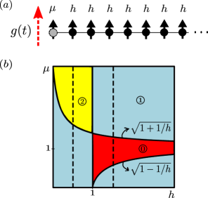
Here, we study the dynamical response of a quantum impurity model, namely, the transverse-field quantum Ising chain with an impurity at its edge [14]. Such an impurity gives rise to a rich phase diagram, where new boundary phases, with up to two localized edge states, emerge, see Fig. 1 below. We show that these edge modes can be accessed through the local control of the impurity and that they hinder the perfect spread of energy and information throughout the chain. In other words, for a suitable finite-time control protocol, excitations can be introduced in the chain through the impurity and a part of them gets trapped in the localized modes. After relaxation, the state describing the remaining excitations can take the form of two entangled qubits, also known as an -state [20]. This opens the possibility of using this setup for information-processing purposes.
Quantum impurity model
We start by describing the system. We consider an interacting quantum system, namely, a spin- chain with open boundary conditions described by the following Hamiltonian,
| (1) |
where are the Pauli matrices (two times the spin- operators) at the site , is the exchange coupling, is the external field magnitude and plays the role of an impurity at the edge. Typically, we will assume that .
This model was introduced and analytically solved in Ref. [14]. In Suppl. Mat. [21], we provide the main details of this solution. The authors of Ref. [14] have shown that the presence of the edge impurity, , produces a new localized mode at the edge , beyond the well-studied Majorana zero mode (MZM) found by Kitaev in the impurity-free case, 111Here we are using the fact that the one-dimensional transverse field quantum Ising chain, after the Jordan-Wigner transformation, can be mapped to a special case of the Kitaev chain [59, 21].. Although slightly different from the transverse field quantum Ising chain, the model in Eq. (1) still undergoes a quantum phase transition, when (for ) is changed and crosses the critical value [14]. For values and , the system is found in the ferromagnetic and paramagnetic phases, respectively.
We highlight that, different from the delocalized (bulk) modes, the two localized edge modes, which hereafter we will denote by , only appear in specific regions of the -phase diagram. Along the line , we recover a physics reminiscent of the Kitaev chain [23]: for , the mode exists (topological phase), while for only the delocalized modes are present (trivial phase). For , the impurity effects appear. The mode is still present for all in the whole ferromagnetic side. Concerning the mode , it can appear in two different regions, depending on the values of . These two regions are: and , and, and .
Figure 1 summarizes this information as follows: in the light blue regions, we only have one localized mode, either or , while in the yellow region we have both localized modes. Finally, in the red region, only the delocalized modes are present. Furthermore, it is important to stress that the modes have very different physical origins. While the mode appears as a direct consequence of an inhomogeneity in real space, the mode has a topological origin, and thus is topologically protected [23, 24, 25]. The real-time dynamics of such localized edge states has been experimentally investigated in [26].
In its diagonal form, the Hamiltonian in Eq. (1) reads,
| (2) |
In the latter equation, summation over includes both localized, , and delocalized, , fermionic modes. The ground state of the Hamiltonian (1) is the fermionic vacuum of , thus for all . In the Suppl. Mat. [21], we provide explicit expressions for the dispersions .
Local control and response function
We now turn to the response of the system to finite-time control localized at . Assuming that the chain is initialized in the ground state (which is a zero-temperature equilibrium state) for arbitrary values of , we apply an impulse at the impurity (where denotes the Dirac delta function).
This perturbation drives the system out of equilibrium and injects energy. An experimentally accessible quantity [27] is the response function,
| (3) |
where is the operator in the Heisenberg representation [28] and . For a sufficiently small value of , the impulse is weak and the response function (3) describes how evolves [29]. In the following, we will show that the local monitoring of the system at the impurity provides important information about the nonequilibrium dynamics of the considered model in its different boundary phases.
Firstly, we consider the short-time behavior of . For very short times , we expand the operator in powers of to obtain , regardless of the point in the -phase diagram. In other words, the short-time behavior of the response function does not distinguish the different boundary phases.
To obtain intermediate and long-time behaviors of , we use the diagonal form (2) of the Hamiltonian . This allows us to perform the calculation of the expectation value in Eq. (3), yielding
| (4) |
The amplitude is the probability of finding the system in the two-particle state after the previously described perturbation. It reads, , with and for the delocalized modes and and for . These are wave functions at the edge, , for the different modes, see Suppl. Mat. [21] to find explicit expressions.
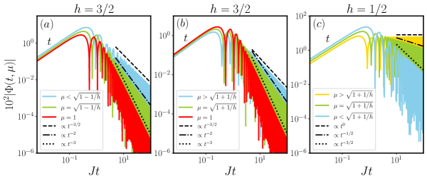
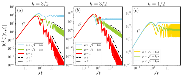
The colored curves in Fig. 2 show Eq. (4) for different values of and for the values of corresponding to the dashed black lines in Fig. 1. Figures 2(a, b) depict the results for the paramagnetic phase, . After an initially linear growth, around , the response function starts to decrease as an oscillatory function with a power-law envelope. In the regions with only one localized mode (the mode), a slower relaxation is observed for , that is, it tends to zero according to . Figures 2(a, b) also show a faster decay of along the boundaries , , even though the mode is absent. Deep inside the red region of Fig. 1, we have a scaling for .
Figure 2(c) shows the results for the ferromagnetic phase, . In the region where only the mode is present, the scaling behavior is exactly the same as that observed in the paramagnetic region (when exists). This tells us that the long-time decay of the response function is not affected by the physical origin of the localized mode. Similarly to the paramagnetic side, the power-law decay changes at the boundary between two different phases. Along , a much slower decay can be observed, that is, . Again, the impurity effects can be detected by the response function even when the mode (which is a direct consequence of it) is absent.
Deep inside the yellow region of Fig. 1, both modes contribute to the response function. In Fig. 2(c), we notice their drastic effect on : it no longer decays to zero but instead oscillates indefinitely. In fact, we obtain
| (5) |
where is the energy of the mode (since the mode has zero energy, ). This coherent oscillation in the long-time limit appears after the delocalized modes undergo relaxation, and so the dynamics is effectively governed only by the two edge modes. In summary, the response function (3) already shows that local monitoring of the system response detects the partial trapping of excitations injected by the local control.
Measuring the spread of correlations
We continue the analysis with a commonly used quantifier of information scrambling [31, 32]. The so-called out-of-time order correlation (OTOC) function is given by
| (6) |
Note that the OTOC (6) depends on the choice of operators [33, 34]. Here, we have chosen a local one to emphasize once again that the local monitoring of the system can give relevant information about the nonequilibrium dynamics. Although similar to the response function (3), it has been shown that the OTOC carries much more information about the spread of quantum correlations, even in non-chaotic systems [35, 16, 36, 37, 38, 39, 40, 41].
It is easy to see that , with
| (7) |
where the out-of-time order structure becomes evident (and denotes the real part). In complete analogy to the response function, the short-time behavior of the OTOC is independent of the region in the -diagram. In fact, one can show that for short times , the OTOC (6) grows according to, , independent of and . This behavior clearly emphasizes the slow, nonexponential spread of information. The impurity model (1) does not support quantum chaos.
To obtain intermediate and long-time behaviors, the calculation of the expectation value in Eq. (6) is more conveniently performed introducing the Majorana representation, , such that the spin operator at the impurity site can be rewritten as , and so . As shown in Ref. [36], we can cast the above expectation value in the form of the Pfaffian of a matrix whose elements are defined by the two-point correlation functions of the Majorana fermions : , . All the details about the calculations are relegated to the Suppl. Mat. [21].
Figure 3 depicts the results for . Regardless of the region in the -diagram, reaches a maximum value around , and for it transits to another behavior. When , we can see how the presence of the impurity modifies the behavior of the OTOC (6). In the paramagnetic phase, Figs. 3(a, b) show three distinct behaviors. First, without localized modes, decays to zero according to , like the response function, cf. Figs. 2(a, b), showing a complete spread of the information as .
The effects of the edge mode on the OTOC can already be seen along the boundaries for . In Figs. 3(a, b), we observe that the information spreads more slowly, , compared to the previous situation.
Inside the regions where only the mode contributes, and , the OTOC is given by the blue curves in Figs. 3(a, b). Interestingly, as time evolves, instead of a power-law decay, the OTOC remains finite for all times. In fact, for large , we have
| (8) |
where const. is a -dependent constant. Hence, is governed by in the regions and . This long-time nonzero value of the OTOC reflects how the localized character of the wave function of the mode around the impurity prevents the perfect spread of the information (and energy) throughout the chain. Similar results have been obtained recently for other systems showing localized edge modes [16, 37, 38, 40] and for a system of interacting electrons in one-dimension [35].
Turning to the ferromagnetic side, , the results can be found in Fig. 3(c). Due to the presence of the mode for all , we see that the OTOC remains finite throughout the ferromagnetic region. For and , is the only localized mode contributing to the OTOC. Since it has zero energy, converges to a finite value, see Fig. 3(c). Finally, when and , both modes are present, and so the OTOC shows an oscillatory long-time behavior. The corresponding analytical result reads, , where is another -dependent constant. The OTOC now oscillates with frequency (half of the frequency found in the paramagnetic phase with a single localized mode). This is essentially the only difference with respect to the case in which was the only contribution.
Emergence of topological -states
The comparison between Figs. 2 and 3 clearly shows the complementary information provided by and . The nonequilibrium steady state characterized by the response and OTOC functions unambiguously exhibits the trapping of excitations in the edge modes. The natural question arises whether the emerging state has useful and interesting properties.
The time evolution of the system, starting from the ground state , after the perturbation , is given by , where (see Suppl. Mat. [21]). Motivated by the correspondence between the existence of the modes , the behavior of the response and OTOC functions, and the decay of coherences induced by the perturbation between states with different occupations of localized and delocalized modes (see Suppl. Mat. [21]), we trace out the delocalized modes to obtain the reduced density operator where denotes the partial trace.
For the remainder of the analysis, we restrict ourselves to the yellow region of Fig. 1. As shown in the Suppl. Mat. [21], then becomes
| (9) |
when written in the basis (in this order), where is the number of excitations in the localized mode.
We see that is an -state [42, 43, 44, 45, 46, 20, 47, 48, 49, 50, 51, 52, 53, 54]. This kind of double-qubit state describes a large and important class of entangled quantum states, ranging from pure Bell states to Werner mixed states [20]. In the present case, the qubits consist of combinations of states having zero, one or two fermionic excitation in the localized modes, namely, and for one qubit and and for another qubit.
For the quantum impurity model (1), the -structure is a consequence of the fact that yields states with two or zero excitation, but also couples the localized and delocalized modes. This allows for part of the excitations to relax and hence granting access to the -dimensional Hilbert space spanned by all possible occupations of the localized modes. Thus, this -state form of cannot exist in the other regions of the -diagram.
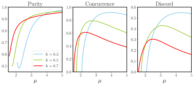
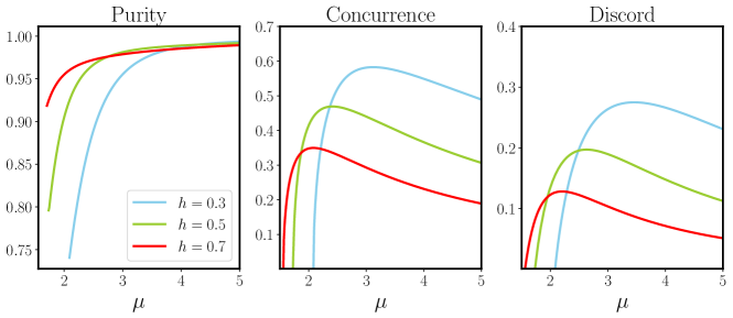
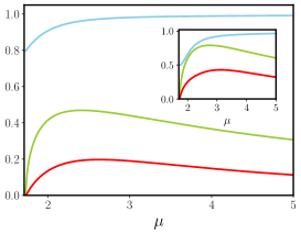
In Fig. 4 we collect information theoretic characterizations [55], such as purity, concurrence, and discord, of (9) as a function of for fixed values of and (see Suppl. Mat. [21] for other values). For , the state is approximately pure and the quantum correlations quantified by the concurrence and discord have a non-monotonic behavior. Interestingly, both concurrence and discord reach a maximal value for small, but finite values of . In the non-perturbative regime, , we see an enhancement of quantum correlations. For very large values of the quantum state becomes essentially classical.
Concluding remarks
In the present analysis, we have shown the emergence of topological -states in a quantum impurity model. This emergence is the consequence of the nonequilibrim response to a local perturbation, and it is heralded by the long-time behavior of the response function and OTOC. In two recent experimental works [56, 57], probing the nonequilibrium dynamics of Rydberg atomic chains, the authors were able to measure very similar OTOC as ours (6).
Finally, it is worth to highlight the similarity of our results and boundary time crystals (BTC) [58]. In our system, like in BTC, while the bulk undergoes relaxation, , where is the equilibrium bulk value before the perturbation, the boundary breaks time-translation symmetry, , where is a periodic function of time. A more detailed analysis of the potential emergence of BTC in impurity models is left for future work.
Acknowledgements.
This work was supported by Conselho Nacional de Desenvolvimento Científico e Tecnológico (CNPq), Brazil, through grant No. 200267/2023-0. M.V.S.B. acknowledges the support of CNPq, under Grant No. 304120/2022-7. E.M. acknowledges the support of CNPq, under Grant No. 309584/2021-3. The work was also financed (M.V.S.B. and E.M.), in part, by the São Paulo Research Foundation (FAPESP), Brazil, Process Number 2022/15453-0. S.D. and M.F.C. acknowledge support from the John Templeton Foundation under Grant No. 62422.References
- Sanders [2017] B. C. Sanders, How to Build a Quantum Computer, 2399-2891 (IOP Publishing, 2017).
- Bruzewicz et al. [2019] C. D. Bruzewicz, J. Chiaverini, R. McConnell, and J. M. Sage, Trapped-ion quantum computing: Progress and challenges, Appl. Phys. Rev. 6, 021314 (2019).
- Wintersperger et al. [2023] K. Wintersperger, F. Dommert, T. Ehmer, A. Hoursanov, J. Klepsch, W. Mauerer, G. Reuber, T. Strohm, M. Yin, and S. Luber, Neutral atom quantum computing hardware: performance and end-user perspective, EPJ Quantum Technology 10, 32 (2023).
- Slussarenko and Pryde [2019] S. Slussarenko and G. J. Pryde, Photonic quantum information processing: A concise review, Appl. Phys. Rev. 6, 041303 (2019).
- Ezratty [2023] O. Ezratty, Perspective on superconducting qubit quantum computing, Eur. Phys. J. A 59, 94 (2023).
- Lahtinen and Pachos [2017] V. Lahtinen and J. K. Pachos, A Short Introduction to Topological Quantum Computation, SciPost Phys. 3, 021 (2017).
- Whaley and Milburn [2015] B. Whaley and G. Milburn, Focus on coherent control of complex quantum systems, New J. Phys. 17, 100202 (2015).
- Soriani et al. [2022] A. Soriani, E. Miranda, S. Deffner, and M. V. S. Bonança, Shortcuts to thermodynamic quasistaticity, Phys. Rev. Lett. 129, 170602 (2022).
- Cavalcante et al. [2024] M. F. Cavalcante, M. V. S. Bonança, E. Miranda, and S. Deffner, Nanowelding of quantum spin- chains at minimal dissipation, Phys. Rev. B 110, 064304 (2024).
- Vasseur et al. [2013] R. Vasseur, K. Trinh, S. Haas, and H. Saleur, Crossover physics in the nonequilibrium dynamics of quenched quantum impurity systems, Phys. Rev. Lett. 110, 240601 (2013).
- Kennes et al. [2014] D. M. Kennes, V. Meden, and R. Vasseur, Universal quench dynamics of interacting quantum impurity systems, Phys. Rev. B 90, 115101 (2014).
- Vasseur et al. [2014] R. Vasseur, J. P. Dahlhaus, and J. E. Moore, Universal nonequilibrium signatures of majorana zero modes in quench dynamics, Phys. Rev. X 4, 041007 (2014).
- Schiró and Mitra [2015] M. Schiró and A. Mitra, Transport across an impurity in one-dimensional quantum liquids far from equilibrium, Phys. Rev. B 91, 235126 (2015).
- Francica et al. [2016] G. Francica, T. J. G. Apollaro, N. Lo Gullo, and F. Plastina, Local quench, majorana zero modes, and disturbance propagation in the ising chain, Phys. Rev. B 94, 245103 (2016).
- Bertini and Fagotti [2016] B. Bertini and M. Fagotti, Determination of the nonequilibrium steady state emerging from a defect, Phys. Rev. Lett. 117, 130402 (2016).
- Dóra et al. [2017] B. Dóra, M. A. Werner, and C. P. Moca, Information scrambling at an impurity quantum critical point, Phys. Rev. B 96, 155116 (2017).
- Bragança et al. [2021] H. Bragança, M. F. Cavalcante, R. G. Pereira, and M. C. O. Aguiar, Quench dynamics and relaxation of a spin coupled to interacting leads, Phys. Rev. B 103, 125152 (2021).
- Javed et al. [2023] U. Javed, J. Marino, V. Oganesyan, and M. Kolodrubetz, Counting edge modes via dynamics of boundary spin impurities, Phys. Rev. B 108, L140301 (2023).
- Larzul et al. [2024] A. Larzul, A. M. Sengupta, A. Georges, and M. Schirò, Fast scrambling at the boundary, arXiv preprint, arXiv:2407.13617 (2024).
- Rau [2009] A. R. P. Rau, Algebraic characterization of x-states in quantum information, Journal of Physics A: Mathematical and Theoretical 42, 412002 (2009).
- [21] Supplemental material.
- Note [1] Here we are using the fact that the one-dimensional transverse field quantum Ising chain, after the Jordan-Wigner transformation, can be mapped to a special case of the Kitaev chain [59, 21].
- Kitaev [2001] A. Y. Kitaev, Unpaired majorana fermions in quantum wires, Physics-Uspekhi 44, 131 (2001).
- Alicea [2012] J. Alicea, New directions in the pursuit of majorana fermions in solid state systems, Reports on Progress in Physics 75, 076501 (2012).
- DeGottardi et al. [2013] W. DeGottardi, M. Thakurathi, S. Vishveshwara, and D. Sen, Majorana fermions in superconducting wires: Effects of long-range hopping, broken time-reversal symmetry, and potential landscapes, Phys. Rev. B 88, 165111 (2013).
- Meier et al. [2016] E. J. Meier, F. A. An, and B. Gadway, Observation of the topological soliton state in the su–schrieffer–heeger model, Nature Communications 7, 13986 (2016).
- Cheneau et al. [2012] M. Cheneau, P. Barmettler, D. Poletti, M. Endres, P. Schauß, T. Fukuhara, C. Gross, I. Bloch, C. Kollath, and S. Kuhr, Light-cone-like spreading of correlations in a quantum many-body system, Nature 481, 484 (2012).
- Coleman [2015] P. Coleman, Introduction to Many-Body Physics (Cambridge University Press, Cambridge, 2015).
- Kubo et al. [1991] R. Kubo, M. Toda, and N. Hashitsume, Statistical Physics II: Nonequilibrium Statistical Mechanics, Vol. 2 (Springer Berlin, Heidelberg, 1991).
- Huang et al. [2024] Y.-H. Huang, Y.-T. Zou, and C. Ding, Dynamical relaxation of a long-range kitaev chain, Phys. Rev. B 109, 094309 (2024).
- Roberts and Swingle [2016] D. A. Roberts and B. Swingle, Lieb-robinson bound and the butterfly effect in quantum field theories, Phys. Rev. Lett. 117, 091602 (2016).
- Touil and Deffner [2024] A. Touil and S. Deffner, Information scrambling – a quantum thermodynamic perspective, EPL (Europhys. Lett.) 146, 48001 (2024).
- Touil and Deffner [2020] A. Touil and S. Deffner, Quantum scrambling and the growth of mutual information, Quantum Sci. Technol. 5, 035005 (2020).
- Tripathy et al. [2024] D. Tripathy, A. Touil, B. Gardas, and S. Deffner, Quantum information scrambling in two-dimensional Bose-Hubbard lattices, Chaos 34, 043121 (2024).
- Dóra and Moessner [2017] B. Dóra and R. Moessner, Out-of-time-ordered density correlators in luttinger liquids, Phys. Rev. Lett. 119, 026802 (2017).
- Lin and Motrunich [2018] C.-J. Lin and O. I. Motrunich, Out-of-time-ordered correlators in a quantum ising chain, Phys. Rev. B 97, 144304 (2018).
- Sedlmayr et al. [2023] M. Sedlmayr, H. Cheraghi, and N. Sedlmayr, Information trapping by topologically protected edge states: Scrambling and the butterfly velocity, Phys. Rev. B 108, 184303 (2023).
- Bin et al. [2023] Q. Bin, L.-L. Wan, F. Nori, Y. Wu, and X.-Y. Lü, Out-of-time-order correlation as a witness for topological phase transitions, Phys. Rev. B 107, L020202 (2023).
- Kheiri et al. [2024] S. Kheiri, H. Cheraghi, S. Mahdavifar, and N. Sedlmayr, Information propagation in one-dimensional chains, Phys. Rev. B 109, 134303 (2024).
- Sur and Sen [2023] S. Sur and D. Sen, Effects of topological and non-topological edge states on information propagation and scrambling in a floquet spin chain, Journal of Physics: Condensed Matter 36, 125402 (2023).
- Muruganandam et al. [2024] V. Muruganandam, M. Sajjan, and S. Kais, Defect-induced localization of information scrambling in 1d kitaev model, Physica Scripta 99, 105123 (2024).
- Ollivier and Zurek [2001] H. Ollivier and W. H. Zurek, Quantum discord: A measure of the quantumness of correlations, Phys. Rev. Lett. 88, 017901 (2001).
- Yu and Eberly [2004] T. Yu and J. H. Eberly, Finite-time disentanglement via spontaneous emission, Phys. Rev. Lett. 93, 140404 (2004).
- Yu and Eberly [2006] T. Yu and J. Eberly, Sudden death of entanglement: Classical noise effects, Optics Communications 264, 393 (2006).
- Santos et al. [2006] M. F. m. c. Santos, P. Milman, L. Davidovich, and N. Zagury, Direct measurement of finite-time disentanglement induced by a reservoir, Phys. Rev. A 73, 040305 (2006).
- Al-Qasimi and James [2008] A. Al-Qasimi and D. F. V. James, Sudden death of entanglement at finite temperature, Phys. Rev. A 77, 012117 (2008).
- Sarandy [2009] M. S. Sarandy, Classical correlation and quantum discord in critical systems, Phys. Rev. A 80, 022108 (2009).
- Ali et al. [2010] M. Ali, A. R. P. Rau, and G. Alber, Quantum discord for two-qubit states, Phys. Rev. A 81, 042105 (2010).
- Galve et al. [2011] F. Galve, G. L. Giorgi, and R. Zambrini, Maximally discordant mixed states of two qubits, Phys. Rev. A 83, 012102 (2011).
- Chen et al. [2011] Q. Chen, C. Zhang, S. Yu, X. X. Yi, and C. H. Oh, Quantum discord of two-qubit states, Phys. Rev. A 84, 042313 (2011).
- Lu et al. [2011] X.-M. Lu, J. Ma, Z. Xi, and X. Wang, Optimal measurements to access classical correlations of two-qubit states, Phys. Rev. A 83, 012327 (2011).
- Quesada et al. [2012] N. Quesada, A. Al-Qasimi, and D. F. James, Quantum properties and dynamics of x states, Journal of Modern Optics 59, 1322 (2012).
- Huang [2013] Y. Huang, Quantum discord for two-qubit states: Analytical formula with very small worst-case error, Phys. Rev. A 88, 014302 (2013).
- Balthazar et al. [2021] W. F. Balthazar, D. G. Braga, V. S. Lamego, M. H. M. Passos, and J. A. O. Huguenin, Spin-orbit states, Phys. Rev. A 103, 022411 (2021).
- Nielsen and Chuang [2010] M. A. Nielsen and I. L. Chuang, Quantum computation and quantum information (Cambridge university press, 2010).
- Xiang et al. [2024] D.-S. Xiang, Y.-W. Zhang, H.-X. Liu, P. Zhou, D. Yuan, K. Zhang, S.-Y. Zhang, B. Xu, L. Liu, Y. Li, and L. Li, Observation of quantum information collapse-and-revival in a strongly-interacting rydberg atom array, arXiv:2410.15455 (2024).
- Liang et al. [2024] X. Liang, Z. Yue, Y.-X. Chao, Z.-X. Hua, Y. Lin, M. K. Tey, and L. You, Observation of anomalous information scrambling in a rydberg atom array, arXiv:2410.16174 (2024).
- Iemini et al. [2018] F. Iemini, A. Russomanno, J. Keeling, M. Schirò, M. Dalmonte, and R. Fazio, Boundary time crystals, Phys. Rev. Lett. 121, 035301 (2018).
- Sachdev [1999] S. Sachdev, Quantum Phase Transitions (Cambridge University Press, Cambridge, 1999).
- Lieb et al. [1961] E. Lieb, T. Schultz, and D. Mattis, Two soluble models of an antiferromagnetic chain, Annals of Physics 16, 407 (1961).
- Yueh [2005] W.-C. Yueh, Eigenvalues of several tridiagonal matrices, Applied Mathematics E-Notes [electronic only] 5, 66 (2005).
Supplemental material
In this Supplementary Material, we provide details on (i) the impurity model, (ii) the OTOC calculations, (iii) the long-time behaviors of the correlation functions, (iv) the reduced density state for the localized edge modes, and (v) the information characterization of our -state.
I Model
The open boundary condition spin- chain with an edge-impurity is described by the Hamiltonian [14]
| (10) |
where are the Pauli matrices at the site and defines the impurity at the edge. After applying the Jordan-Wigner transformation [60, 59], and , the Hamiltonian of Eq. (10) reads
| (11) |
where and . Following [60, 61, 14], the Hamiltonian (11) can be brought to the form
| (12) |
where represents the Bogoliubov transformation [60]. are fermionic degrees of freedom: for the localized modes, and for the delocalized ones. To guarantee the correct fermionic anti-commutation relations, and , the wave functions and need to satisfy (in matrix notation): and , where is the identity matrix, is the null matrix and T denotes the transpose operation. The inverse transformation reads, . In what follows, we will work with the quantities, and .
As discussed in the main text, the localized edge modes only appear in specific regions of the -phase diagram (see Fig. 1(b) in the main text). For the mode, these regions are: for all and for . The energy and wave functions of this mode are,
| (13) | |||||
where, hereafter, we use the superscript to label the localized mode . The mode exists in the entire region (topological phase of the Kitaev chain [23]). For this mode, we have
| (14) | |||||
where is the sign function. Notice that in the limit , .
Finally, for the delocalized modes , we have
| (15) | |||||
In the continuum limit, we can take as usual [14]. We see that the system gap closes at , independently of , where the system undergoes a quantum phase transition [59].
I.1 Majorana representation
The model of Eq. (10) can be rewritten in terms of Majorana fermions. As discussed in the main text, this representation is useful for the calculation of the OTOC.
Decomposing the spinless fermionic operators in the basis, and , where and are Majorana fermions, , and , the Hamiltonian of Eq. (11) is recast as
| (16) |
In particular, when , we can see that the Majorana fermion totally decouples from the rest of the chain, , and thus it becomes a Majorana zero mode. For , this mode is reminiscent of Kitaev’s zero mode, while for , it is simply an impurity effect.
II OTOC calculation
Here, we are interested in the OTOC,
| (17) | |||||
where and denotes the real part. Using the Majorana representation discussed before, we can rewrite so that
| (18) |
The above OTOC can be calculated applying Wick’s theorem since and are linear combinations of and . However, as shown in reference [36], this expectation value can be cast in the form of a Pfaffian of a matrix ,
| (19) |
For our case,
| (20) |
where we defined the matrices
| (21) | |||||
| (22) |
Here, , where , and is the identity matrix. Notice that .
| Region | ||
|---|---|---|
| and | Eq. (8) | |
| and | ||
| and | ||
| and | ||
| and | ||
| and | Eq. (5) |
Since, like the determinant, the Pfaffian is invariant under the addition of rows and columns, we obtain
| (23) |
where now
| (24) |
and is the null matrix. Performing the calculation, we find [36]
| (25) | |||||
where denotes the imaginary part.
The two-point Majorana correlation functions in the above expression, , are given by
| (26) |
where the above summations include both the delocalized and the localized modes, and we used the notation .
III Stationary phase approximation (SPA)
The long-time power-law behaviors observed for the response function and the OTOC (see Figs. 1 and 2 in the main text) can be understood by applying the stationary phase approximation (SPA) [30].
III.1 Response function
In the limit , the summation over the bulk modes in Eq. (4) is converted to an integral. In the red region of Fig. 1(b), where we only have delocalized modes, the response function is given by
| (27) |
The long-time limit () of is obtained by performing the integration of expanded near the extreme points of : [see Eq. (15)]. Expanding around the points gives us , which produces a decay faster than . If we expand around (or, equivalently, around ), we obtain . This leads to, , which agrees with the numerical calculation of Eq. (4), see Fig. 2(a, b).
When only one of the localized modes is present (and far from the boundaries), besides the contribution in Eq. (27), we also have the term . For the latter, obviously the extreme points are , and both of them give the same result, (when expanded around , we have done a -translation). Thus, . At the boundaries, and , behaves as around . Then, . However, at the boundary and , the mode contributes, making around . This produces the slower decay seen in Fig. 2(c), .
III.2 OTOC
As we saw in the Sec. II, to calculate we need to know the two-point Majorana correlation functions, , see Eq. (25). The long-time behavior of can be extracted from the SPA discussed above. In the red region of Fig. 1(b), from Eq. (15) we obtain around . Thus, (see Eq. (26)). This leads to . At the boundaries and , (for we have expanded around while for around ). Then, , which produces .
In table 1 we summarize all the results for the asymptotic behaviors of and .
IV Reduced state for the localized modes
For the system initially prepared in its ground state within the yellow region of Fig. 1(b), we turn on the impulsive perturbation . The system state at time will be given by
| (28) |
where , with , and is the time ordering operator. Using the Dirac delta function property,
| (29) |
where it was considered that . Thus, the system density operator reads,
| (30) | |||||
The density operator , being the state of the full system, provides the time evolution of any average value, in particular, the local magnetization of the impurity, given by . However, can also be obtained from the response function (3) in the perturbative regime and, as shown in Fig.2(c) of the manuscript, its long-time behavior has persistent oscillations when the two localized modes are present. Next, we show that this is a signature of the -state in the reduced density operator of the localized modes and that couplings (in the sense of non-diagonal matrix elements of ) introduced by the perturbation between the edge and bulk modes with different number of excitations in the later ones decay in the long-time limit. To see this, we express as follows,
| (31) | |||||
where and are two Fock states: , being (with ) the localized edge modes part and (with ) the delocalized modes part. Because creates zero or two excitations (), the non-zero terms in the above expression are terms where and differ by zero or two excitations. These excitations can occupy edge or bulk modes. However, in the long-time limit, , not all of those terms will survive due to the presence of high oscillatory factors. For instance, let us analyze the matrix elements , where and , being the delocalized fermionic vacuum, . The last term of Eq. (30) gives us (the others are zero),
Thus, the sum over all states like this in Eq. (31), is a sum of high oscillatory terms, which goes to zero when . Therefore, the only surviving coherences in the long-time limit are those corresponding to Fock states with equal number of excitations in the bulk modes. In the long-time limit, the relevant content of is hence concentrated in the subspace spanned by the states with 0, 1 and 2 excitations in the edge modes, i.e., in the reduced density operator obtained by
| (33) | |||||
After performing the above calculation, we find
| (34) | |||||
In the matrix representation this reads,
| (35) |
where
| (36) |
The functions in the above expressions are
Notice that is time-independent.
V Purity, entanglement and discord
The purity is obtained as usual from , with given by Eq. (9). The entanglement measure is given by the concurrence, , which can be obtained in terms of the matrix elements of the -state as follows [48]
Finally, the discord is obtained following Refs. [48, 53]. In Figs. 5 and 6 we show the results for these three quantities assuming different values.