On Learning Representations for Tabular Data Distillation

Abstract

Dataset distillation generates a small set of information-rich instances from a large dataset, resulting in reduced storage requirements, privacy or copyright risks, and computational costs for downstream modeling, though much of the research has focused on the image data modality. We study tabular data distillation, which brings in novel challenges such as the inherent feature heterogeneity and the common use of non-differentiable learning models (such as decision tree ensembles and nearest-neighbor predictors). To mitigate these challenges, we present TDColER, a tabular data distillation framework via column embeddings-based representation learning. To evaluate this framework, we also present a tabular data distillation benchmark, TDBench. Based on an elaborate evaluation on TDBench, resulting in 226,890 distilled datasets and 548,880 models trained on them, we demonstrate that TDColER is able to boost the distilled data quality of off-the-shelf distillation schemes by 0.5-143% across 7 different tabular learning models.

1 Introduction

Dataset distillation or dataset condensation is the process of creating a small set of extremely informative samples (usually synthetic) from a large dataset such that a model trained on this set will have predictive performance comparable to that of a model trained on the original large dataset (Wang et al., 2020; Yu et al., 2023). First, data distillation reduces data storage costs and can mitigate the privacy and copyright concerns involved in keeping around (and continuously utilizing) large amounts of raw data. Furthermore, the reduction in the data size implies a lower computational cost of model training, especially when multiple models need to be trained on any given dataset. The above advantages of dataset distillation also facilitate various applications. Continual learning, where we need to learn new tasks while avoiding forgetting older tasks sequentially, often makes use of a “replay buffer” of old task data to be used while learning new tasks to mitigate forgetting of the older tasks (Rolnick et al., 2019). Dataset distillation reduces the memory overhead of this replay buffer, allowing learning of a larger number of tasks without forgetting (Tiwari et al., 2022; Rosasco et al., 2022).

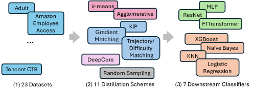
Figure 1: Overview of TDBench. The benchmarking suite allows for flexible choice of datasets, distillation schemes, and downstream models that enables for modular evaluation of any new distillation method.

In federated learning, we need to train a model using data spread across multiple clients without ever moving the data between clients and reducing the communication overhead. Dataset distillation generates compact yet private synthetic data from the client data that can be safely exchanged for communication-efficient model training (Song et al., 2023; Goetz & Tewari, 2020; Zhou et al., 2020).

While dataset distillation has been widely studied for image datasets (Cui et al., 2022; Yu et al., 2023), the equally important application to other data modalities is limited. The problem of tabular data distillation has received very little attention, though many real-world learning problems and applications involve tabular data (Guo et al., 2017; Clements et al., ; Borisov et al., 2024). Various image data distillation schemes have been proposed in the literature, but their application to tabular data is not straightforward. First, all image data distillation schemes rely on the choice of a differentiable “backbone model.” While differentiable neural network-based schemes are standard for images, a wide variety of non-differentiable models are used with tabular data, such as decision tree ensembles, nearest-neighbor models, and kernel machines. Second, almost all data distillation methods for images generate distilled data in the original pixel space. While pixels are homogeneous raw features of an image, the features in tabular data can be extremely heterogeneous, creating a mismatch between what the image data distillation methods are designed for and what we have as an inherent property of tabular data. Finally, it is standard to use vision-specific data augmentation schemes (such as rotation, reflection, cropping, and translation) to train the model on the distilled image data. Such standard augmentations are not available for tabular data, thus creating another discrepancy in the expected conditions for the problem.

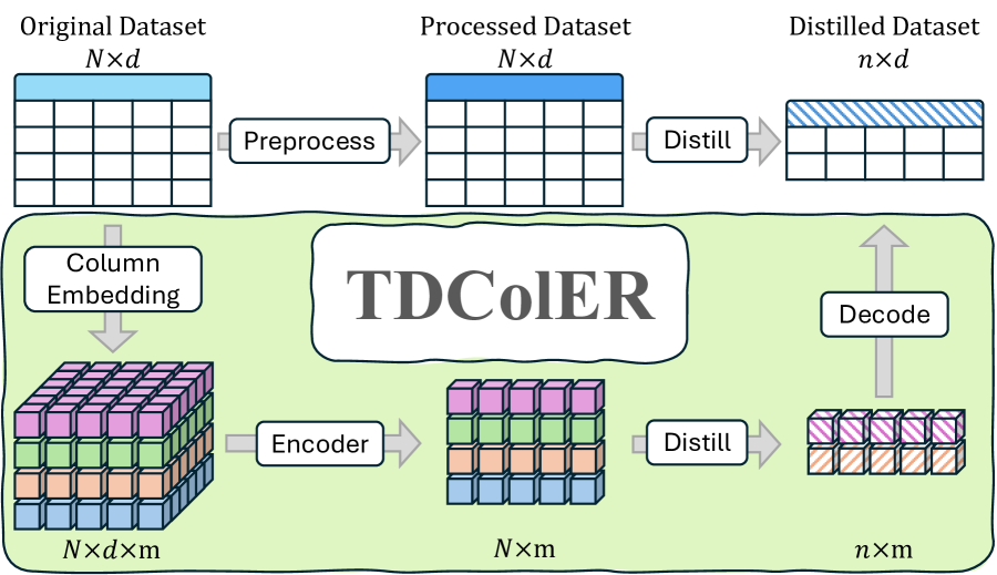
(a) Overview of TDColER. The top describes a vanilla distillation scheme that only uses standard preprocessing techniques before distillation. The highlighted box describes the proposed TDColER, which uses column embeddings after such preprocessing and encoder-decoder architectures to generate rich compact representations.

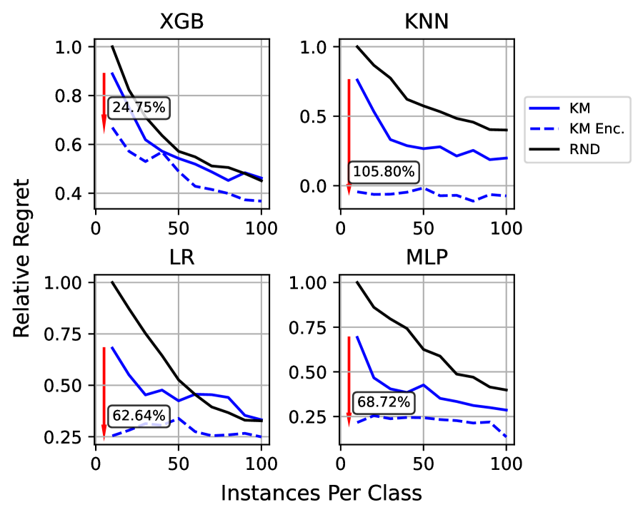
(b) Snapshot of downstream classifiers’ performance increase when trained on data distilled $k$-means with and without TDColER. Throughout our experiments, we observe a performance increase from 0.5% to as large as 143%.

Figure 2: Proposed approach – TDColER: Tabular Distillation Via Column Embeddings based Representation Learning

Our contribution.

In this paper, we study tabular dataset distillation and present a novel scheme to enhance the distilled data quality of multiple off-the-shelf data distillation schemes across various datasets, models, and distillation sizes. Specifically, we make the following contributions:

• We propose Tabular Distillation via Column Embeddings based Representation Learning or TDColER that can utilize modern neural-network architectures such as Transformers and graph neural networks to generate rich compact representations. TDColER improves the quality of distilled data compared to existing distillation schemes. Figure˜2(a) provides an overview of our proposed TDColER.

• We present TDBench, a Tabular Distillation Benchmark with 23 tabular datasets, 7 model classes, and 11 distillation schemes. We present an overview of TDBench, an extensible and modular framework for measuring various aspects of data distillation on tabular data, in fig.˜1.

• With the elaborate evaluation of our proposed TDColER on TDBench, resulting in over 226,890 distilled datasets and 548,880 model trainings, we show that, on aggregate across all datasets, TDColER improves upon direct application of off-the-shelf distillation method on tabular data by 0.5-143% in terms of the distilled data quality across all models at the smallest distillation of 10 instances-per-class. Figure˜2(b) presents a snapshot of our results.

• Based on our thorough evaluation, we present various insights regarding tabular dataset distillation, such as (i) $k$-means clustering in the learned representations make for an extremely favorable distillation scheme, (ii)  transformer-based tabular data representations obtain the highest distilled data quality on aggregate, while (iii) graph neural network based tabular data representations perform slightly worse than transformers but are significantly more parameter efficient.

1.1 Related Work

Dataset distillation was introduced by Wang et al. (2020) as a bilevel optimization problem (Feng et al., 2024) and has been widely studied in the context of image data distillation. Most methods can be categorized into approaches that match the original data by (i) backbone model performance, (ii) backbone model parameters, or (iii) backbone representation distributions (Yu et al., 2023). Wang et al. (2020) minimized performance differences between the original and distilled data, while Nguyen et al. (2021) introduced kernel-induced points (KIP) using kernel ridge regression with a neural tangent kernel (Jacot et al., 2018). Alternatively, methods have focused on parameter or gradient matching (Zhao et al., 2021; Lee et al., 2022; Jiang et al., 2023; Cazenavette et al., 2022). Gradient matching (Zhao et al., 2021) aligns model gradients between original and synthetic data, while trajectory matching (Cazenavette et al., 2022) minimizes discrepancies between entire training trajectories. Other approaches include distribution matching (Zhao & Bilen, 2023), which aligns per-class means, and cross-layer feature embedding matching (Wang et al., 2022). However, the abovementioned methods rely on differentiable backbones, limiting cross-architecture generalization (Cui et al., 2022; Nguyen et al., 2021). As a result, research has focused primarily on images, leaving tabular data distillation largely unexplored (Medvedev & D’yakonov, 2021). We address this gap by proposing a more general distillation framework.

Dataset distillation aligns with coreset selection (Feldman, 2020), which aims to reduce data size, typically selecting real data instances (potentially risking privacy). In contrast, distillation generates synthetic data beyond the real data manifold. Notably, coreset selection is a subset of dataset distillation, where the synthetic data lies on the real data manifold. Generative modeling (Goodfellow et al., 2020; Kingma & Welling, 2013) is another related area, usually focused on generating realistic data. In dataset distillation, the goal is to generate informative rather than realistic samples. Recently, Cazenavette et al. (2023) demonstrated how generative modeling can be used to seed the dataset distillation process, arguing that distillation methods should be applied to a latent representation instead of the pixel space. This is aligned with our proposal, in which we demonstrate that distillation in the latent space is critical to obtaining meaningful distilled data quality with tabular datasets. However, the proposed Generative Latent Distillation(GLaD) scheme is very focused on generative vision models, requiring a careful choice of the latent representation from within the model for trade-off in realistic distilled data or expressivity, thus limiting cross-architecture generalization.

Cui et al. (2022) benchmarked several distillation methods and found trajectory matching (Cazenavette et al., 2022) to be most effective, followed by KIP (Nguyen et al., 2021). Coreset methods, like $k$-means clustering, also outperformed many model-based distillation techniques, which we corroborate. We focus on GM and KIP due to the high computational overhead of trajectory matching and omit data augmentation due to its limited applicability to tabular data. As noted before, data augmentation is not standard with tabular data, and we do not consider it in our evaluation with TDBench.

2 Table Distillation

Data distillation has been primarily studied in the context of images where each data point is composed of a homogeneous set of features – pixels – and the downstream models are neural networks. The two main distinctions with tabular data distillation are: (i) Feature Heterogeneity: Features in tabular data are usually heterogeneous and can have vastly different meanings, making it challenging to generate appropriate feature aggregations as usually done with neural networks. This is further exacerbated by the common presence of missing values.

$\tilde{S}\leftarrow\left\{(P(x),y)\,\forall(x,y)\in S\right\}$   // Preprocess $R\leftarrow F(\tilde{S})$   // Distill return $R$ Algorithm 1 Distill original data $S$ with $N$ samples given a preprocessor $P:\mathbb{R}^{r}\times{\mathbb{C}}^{c}\to\mathbb{R}^{D}$ and a distiller $F:\mathbb{R}^{N\times D}\times Y^{N}\to\mathbb{R}^{n\times D}\times Y^{n}$.

(ii) Model Agnosticity: For tabular data, the downstream model that will use the distilled data can be quite varied, with decision-tree-based models often being quite successful (Grinsztajn et al., 2022), while linear and nearest-neighbor models are used for interpretability. Various increasing competitive neural-network-based models have also been developed for tabular data (Borisov et al., 2024; Gorishniy et al., 2021; McElfresh et al., 2023; Grinsztajn et al., 2022). However, in the most common cases, we cannot assume that the downstream model is differentiable and thus will be unable to perform a downstream model-specific distillation via the common bilevel formulation of the problem. The distillation has to be model-agnostic, which means that we have to retain as much of the information in the original data as possible since we do not know a priori what information the downstream model might leverage.

We will consider a classification dataset $S=\{(x_{1},y_{1}),\ldots,(x_{N},y_{N})\}$ with $N$ samples, $r$ numerical features and $c$ categorical features, and $L$ labels, where each $x_{i}\in\mathbb{R}^{r}\times{\mathbb{C}}^{c}$ and $y_{i}\in Y=\{1,\ldots,L\}$. Following Cui et al. (2022), we only consider classification tasks in this work, but it should be noted that regression can be easily added into our framework. Note that features may contain missing values. After appropriate preprocessing steps to convert the categorical variables to numerical ones and imputing the missing values, we can directly apply some existing distillation schemes such as KIP (Nguyen et al., 2021) or GM (Zhao et al., 2021). This procedure is sketched in Algorithm 1.

2.1 Representation Learning via Column Embedding

A key ingredient in the development of neural networks for tabular data is the use of column embeddings. First developed for categorical features, the idea is to learn an embedding for each of the categories in a categorical feature (Guo & Berkhahn, 2016). This embedding would replace the one-hot encoded numerical representation of the categories and be used in conjunction with the (appropriately scaled and imputed) numerical features in standard and custom feed-forward networks (FFNs) (Borisov et al., 2024). Column embeddings for numerical data were developed to use more standard modern architectures such as graph neural networks (GNNs) and Transformers. As with categorical data, each numerical value in a numerical feature of the table would be converted into a learnable embedding. Thus, more precisely, a sample (row) in a table with $r$ numerical features and $c$ categorical features is now represented as a set of $(r+c)$ embeddings in $\mathbb{R}^{m}$ each of size $m$ (where $m$ is a user-specified hyperparameter), thus effectively as the $(m\times(r+c))$ matrix.

Encoder Architectures.

Given the $\mathbb{R}^{m\times(r+c)}$ representation of a row (sample) using column embeddings, our goal is to learn a more compact yet faithful representation of a row. One simple strategy is to concatenate all the $(r+c)$ column embeddings into a single vector in $\mathbb{R}^{m(r+c)}$ of size $m(r+c)$ and input it into an FFN which projects it down to a lower dimensionality (fig.˜10). However, one of our main motivations for using column embeddings is to leverage the capabilities of more modern architectures. For a given row, the $(r+c)$ column embeddings can be treated as initial token embeddings that are progressively updated through multiple Transformer blocks as described by Gorishniy et al. (2021). Using a dummy [CLS] token, the above process can create a $m$-dimensional representation of the row (fig.˜13). An alternate procedure is to represent a table as a bipartite graph between columns and rows (with column values and rows as vertices) and utilize the column embeddings as representations for the column vertices (Wu et al., 2021). Then, the row embeddings are obtained by filling in representations for the row vertices via multiple rounds of message passing in a multi-layered GNN (fig.˜11). For our purposes, we consider all three architectures – FFN, Transformer and GNN – as encoders that project the $\mathbb{R}^{m\times(r+c)}$ representation of row into an embedding in $\mathbb{R}^{m}$. While categorical column embeddings are standard, there are multiple techniques for numerical column embeddings (Gorishniy et al., 2021; 2022). We discuss and ablate the effect these different schemes have in section˜B.2.

Learning Objective.

Our goal is to retain as much information regarding the original data in the learned representation as possible. The need for high-fidelity learned representations is critical because we do not assume anything regarding the downstream model, which will be trained with the distilled data. Thus, we try to reconstruct the original data from the learned representation as well as possible. Formally, given column embeddings $C:\mathbb{R}^{r}\times{\mathbb{C}}^{c}\to\mathbb{R}^{m\times(r+c)}$, and an encoder $\phi:\mathbb{R}^{m\times(r+c)}\to\mathbb{R}^{m}$, we utilize a decoder $\psi:\mathbb{R}^{m}\to\mathbb{R}^{r}\times{\mathbb{C}}^{c}$ to reconstruct the original data, and solve the following optimization problem:

$$\min_{C,\phi,\psi}\sum_{(x,y)\in S}\ell\left(x,\psi(\phi(C(x)))\right),$$ (1)

where $\ell(\cdot,\cdot)$ is a reconstruction error (RE). Note that the above representation learning does not use the label information in the data $S$. This representation learning framework allows us to infuse class information in the representations while ensuring no loss of original information. Thus, after obtaining the column embeddings $C$, encoder $\phi$ and decoder $\psi$ by solving eq.˜1, we fine-tune the encoder by learning a classifier $f:\mathbb{R}^{m}\to Y$ on top of the learned representations while keeping the reconstruction loss low:

$$\min_{C,\phi,\psi,f}\sum_{(x,y)\in S}\ell(x,\psi(\phi(C(x)))+\alpha\mathcal{L}(y,f(\phi(C(x)))),$$ (2)

where $\mathcal{L}(\cdot,\cdot)$ is the downstream learning loss function, and $\alpha>0$ is a hyperparameter balancing the classification and reconstruction quality. Section˜A.4.2 discusses this procedure in more detail.

$C,\phi,\psi\leftarrow$ solve eq.˜1   // minimize RE $C,\phi,\psi,f\leftarrow$ solve eq.˜2   // fine-tune $\tilde{S}\leftarrow\{(\phi(C(x)),y),(x,y)\in S\}$   // Encode $\tilde{R}\leftarrow F(\tilde{S})$   // Distill in latent space $R\leftarrow\{(\psi(x),y),(x,y)\in\tilde{R}\}$   // Decode return $R,\tilde{R},C,\phi,\psi$ Algorithm 2 TDColER: Distill dataset $S$ with $N$ samples given distiller $F:\mathbb{R}^{N\times m}\times Y^{N}\to\mathbb{R}^{n\times m}\times Y^{n}$, and learnable column embeddings $C:\mathbb{R}^{r}\times{\mathbb{C}}^{c}\to\mathbb{R}^{m\times(r+c)}$, encoder $\phi:\mathbb{R}^{m(r+c)}\to\mathbb{R}^{m}$, decoder $\psi:\mathbb{R}^{m}\to\mathbb{R}^{r}\times{\mathbb{C}}^{c}$, classifier $f:\mathbb{R}^{m}\to Y$.

Complete Distillation Pipeline.

After the column embeddings $C$, encoder $\phi$ and decoder $\psi$ are learned (with eq.˜1) and fine-tuned (with eq.˜2), we convert the input features of the whole original dataset (with $N$ samples) into the learned representations in $\mathbb{R}^{m}$ using $C$ and $\phi$ and apply the aforementioned distillation schemes to this dataset ($N$ samples in $\mathbb{R}^{m}$) to get $n$ distilled samples in $\mathbb{R}^{m}$. At this point, we decode the distilled samples into the original representation using $\psi$. This whole pipeline is summarized in Algorithm 2. Note that the distillation with the learned representation in $\mathbb{R}^{m}$, and the availability of the decoder $\psi$, allows us to have two versions of the distilled data – one in the learned representation ($\tilde{R}$ in Algorithm 2, Line 4), and one in the original representation ($R$ in Algorithm 2, Line 5). We can choose the appropriate distilled set based on the downstream application: If we require the distilled data to be obfuscated with no explicit correspondence to the original features, we can use $\tilde{R}$. In this setting, we are required to have the column embeddings $C$ and the encoder $\phi$ during inference with the downstream trained model to map the test points into the appropriate representation. If we require the distilled data and the model trained on it to be interpretable in terms of the original features, we should use the distilled set $R$ in the original representation. In this case, we do not need the column embeddings or the encoder during inference.

Remark 1.

Our contribution is a novel representation learning and distillation pipeline for model-agnostic tabular data distillation utilizing existing distillation schemes, column embeddings, and network architectures such as transformers and GNNs. In our thorough empirical evaluations, we will demonstrate the distilled data quality boost from this pipeline across multiple datasets and downstream models.

3 Evaluation Benchmark

To thoroughly evaluate the various configurations of the proposed distillation pipeline, we establish a comprehensive benchmark suite with a varied set of datasets and downstream models, evaluating the pipeline at various levels of distillation sizes. With 3 encoder architectures, 12 distillation schemes (including variants), 20+ datasets, 7 downstream models, 10 distillation sizes, 5 repetitions per distillation pipeline, and model training, we have generated over 226,890 distilled datasets and trained over 548,880 individual downstream models 

Datasets.

We consider 23 datasets from OpenML (Vanschoren et al., 2013) with the number of samples varying from 10,000 to over 110,000, and number of features varying from 7 to 54. Instead of investigating a few large datasets, we choose to incorporate more datasets to generalize the findings across a wider range of datasets. The datasets are chosen to be diverse in terms of the number of samples, features, and the type of features (numerical, categorical, or mixed). There are 14/23 datasets with only numerical features, 2/23 with only categorical features, and 7/23 with both numerical and categorical features. All these datasets correspond to binary classification problems. Class imbalance is a common feature of tabular datasets (Johnson & Khoshgoftaar, 2019; Thabtah et al., 2020), and we focus on binary classification to carefully study the effect of class imbalance on the distilled data quality. There are 9/23 almost perfectly balanced datasets and 10/23 datasets with a ratio of close to 1:2 between the smaller and larger classes, with the worst imbalance ratio smaller than 1:15. Note that while we only consider binary classification datasets, the distillation pipelines are natively applicable to multi-class classification problems.

Distillation Methods.

Given our aforementioned desiderata for model-agnosticity, we have the following existing distillation schemes available, which take as input the set $S$ of $N$ samples and output a set $R$ of $n\ll N$ distilled samples (further details regarding implementation of each distillation method is provided in section˜A.5.2):

• $k$-means Clustering (KM) finds $n/L$ clusters for each of the $L$ classes to produce a total of $n$ distilled samples using Lloyd’s $k$-means algorithm (Lloyd, 1982). We consider two variations here by (i) using the Euclidean center of each cluster to generate a synthetic sample or (ii) choosing the closest real point to the Euclidean center of each cluster. That is, $R$ comprises $n/L$ cluster centers (or closest real points) for each of the $L$ classes.

• Agglomerative Clustering (AG) (Müllner, 2011) again generates $n/L$ clusters for each of the $L$ classes is similar to $k$-means. We use the Ward linkage scheme with the Euclidean distance metric. Similar to $k$-means, we generate (i) synthetic samples by using the Euclidean center of a cluster or (ii) real samples that are closest to the cluster centers.

• Kernel Induced Points (KIP) (Nguyen et al., 2021) uses the neural tangent kernel (NTK) (Jacot et al., 2018) of a wide neural network and kernel ridge regression to produce a distilled set of samples. Given the feature matrix $X\in\mathbb{R}^{N\times D}$ and the label vector $\mathbf{y}\in Y^{N}$, KIP learns the distilled feature matrix $\bar{X}\in\mathbb{R}^{n\times D}$ and label vector $\bar{\mathbf{y}}\in Y^{n}$ by solving the following problem:

  $$\min_{\bar{X},\bar{\mathbf{y}}}\mathcal{L}\left(\mathbf{y},K_{X\bar{X}}(K_{\bar{X}\bar{X}}+\lambda I)^{-1}\bar{\mathbf{y}}\right),$$ (3)

  where $\mathcal{L}$ is the downstream learning loss function, $K_{X\bar{X}}\in\mathbb{R}^{N\times n}$ is the NTK matrix between $X$ and $\bar{X}$, $K_{\bar{X}\bar{X}}\in\mathbb{R}^{n\times n}$ is the NTK matrix of $\bar{X}$ with itself, and $\lambda>0$ is a regularization hyperparameter for the kernel ridge regression. Essentially, we are learning a set of synthetic samples such that the predictions made on the original dataset features using the distilled dataset via kernel ridge regression match the original labels.

• Gradient Matching (GM) (Zhao et al., 2021) produces the distilled set $R$ for a given “backbone model” $M_{\theta}$ (parameterized by $\theta$) by directly optimizing for $R$ to induce model parameter gradients that are similar to the gradients obtained while training $M_{\theta}$ on the full dataset $S$. Given a distance metric $D(\cdot,\cdot)$, and a distribution $P_{\theta_{0}}$ over the random model parameter initializations $\theta_{0}$, the distillation problem tries to minimize the distance between the model gradients computed on the full and distilled datasets over the $T$ steps of model learning as follows:

  $$\min_{R}\mathbb{E}_{\theta_{0}\sim P_{\theta_{0}}}\left[\sum_{t=0}^{T-1}D\left(\nabla_{\theta}\mathcal{L}(\theta_{t};S),\nabla_{\theta}\mathcal{L}(\theta_{t};R)\right)\right],$$ (4)

  where $\mathcal{L}(\theta;S)$ is the loss of the model $M_{\theta}$ on the original full dataset $S$, $\mathcal{L}(\theta;R)$ is the loss of $M_{\theta}$ evaluated on $R$, and the model parameters $\theta_{t}$ are updated at $\theta_{t+1}\leftarrow\theta_{t}-\eta_{\theta}\nabla_{\theta}\mathcal{L}(\theta_{t};S)$ via gradient descent with a learning rate $\eta_{\theta}$ using the full original dataset.

We consider KIP and GM as representatives from previous data distillation literature that are model-agnostic and model-centric, respectively. Section˜A.5.1 further discusses our choice of distillation methods considered in this work. However, based on the weaker downstream performance of these methods in our initial experiments, we later included more recent methods from computer vision, such as trajectory-based matching Cazenavette et al. (2022) and its evolved version difficultiy-based matching Guo et al. (2023), and 4 representative NN-based coreset selection methods from DeepCore Guo et al. (2022). All the above distillation schemes require the data to be preprocessed into a numerical form, and can be used in Algorithm 1 to distill tables. But, as we will see, this is not a very useful scheme. Our evaluation of TDColER on TDBench will demonstrate how the performance of these distillation schemes are boosted via representation learning.

To study the ability of the distillation pipeline to generate really small but useful distilled datasets, we consider extremely small distilled datasets with 10-100 instances per class (IPC), corresponding to a distillation fraction of the order of 0.1-1.0% on the smallest datasets, and 0.01-0.1% for the largest datasets. This is comparable to the compression ratio of 0.02-1% used in Cui et al. (2022) and Cazenavette et al. (2023).

Downstream models.

We consider 7 downstream models to evaluate the distilled data quality. We consider the Nearest-Neighbor Classifier (KNeighbors), Logistic Regression (LR), Gaussian Naive Bayes (GNB), and the Multi-Layered Perceptron (MLP) from the scikit-learn library (Pedregosa et al., 2011). We also consider the popular XGBoost ensemble of gradient-boosted decision trees (XGB) (Chen & Guestrin, 2016). We include two recent neural network models for tabular data, the ResNet and the FTTransformer models (Gorishniy et al., 2021). Since our distillation pipeline is deliberately model-agnostic, we train these models on the distilled data using the default hyperparameters of the corresponding libraries. We also consider a hyperparameter optimization (HPO) use case using the distilled datasets in our evaluations, which can be found in Appendix 4.

Evaluation metric.

To have a standardized way to quantify the quality of the distilled data across different models and datasets, we use the notion of relative regret which compares the model’s balanced accuracy score when trained on the full, distilled and randomly sampled data points. Precisely, the relative regret is defined as $\nicefrac{{(A_{F}-A)}}{{(A_{F}-A_{R_{10}})}}$, where $A_{F}$ is the balanced accuracy of the model trained on the full training set, $A_{R_{10}}$ is the balanced accuracy on the same test set when trained on 10 random samples per class averaged over 5 random repetitions, and $A$ is the balanced accuracy of the model when trained on the distilled dataset over random 5 repetitions. A relative regret of 1 matches the performance of random sampling at IPC=10, and a relative regret of 0 matches the performance of the model trained on the full dataset (which is usually the gold standard) – lower relative regret implies higher distilled data quality .

4 Results Analysis

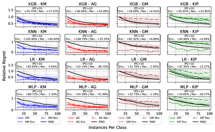
Figure 3: Change in relative regret of downstream classifiers when trained on distilled data over IPC $\in[10,100]$, aggregated over datasets and encoder architectures. Lower is better. Each column corresponds to a downstream classifier, and each row represents a representation scheme – original, encoded (Enc.), and reconstructed (Rec.). Data distilled by clustering methods (AG, KM) in the encoded space show the best performance for all classifiers. In many cases, using the encoded representation as the final output yields a performance comparable to using the original representation. Figure˜14 shows a more detailed version of this plot that includes FTTransformer and ResNet.

Table 1: Average rank and median relative regret of distillation pipelines that use the latent space of different encoder architectures evaluated at IPC=10, grouped over all datasets and classifiers.

Encoder	Mean Rank	Median R.R.
TF	4.1176	0.9439
FFN	4.3407	0.9746
GNN	4.2243	0.9695
TF*	2.3591	0.6149
FFN*	3.3652	0.8082
GNN*	2.5931	0.7135

In this section, we present the analysis of the results obtained from our benchmarking experiments. For the sake of brevity, we will use the following acronyms – Instances Per Class: IPC, $k$-means: KM, agglomerative: AG, gradient matching: GM, kernel inducing points: KIP, feed-forward neural network: FFN, graph neural network: GNN, transformer: TF. Additionally, the supervised-fine-tuned variant of the autoencoder will be marked with a *. For example, the results of Algorithm 2 with a transformer architecture for $\phi$ as TF*, whereas TF denotes the version that skips line 2 of Algorithm 2 to highlight the importance of the supervised fine-tuning.

How beneficial are the learned representations for distillation?

As the first step of our analysis, we examine the performance difference between pipelines that use encoder’s latent space and those that do not. To fully understand the effect of our latent space projection step, we analyze our results from two angles: 1) Is it better to distill in the latent or original space? 2) If latent space is better, is it better to decode the data back to the original space or stay in the latent space?

Figure˜3 shows the relative regret score of distillation methods under different data representation schemes. We start by examining the downstream performance difference between pipelines that use the latent space to distill in vs. ones that do not (Algorithm 2 vs. Algorithm 1). The results show that using the latent space is highly beneficial in most cases with lower IPC values. This trend is most apparent in classifiers such as KNN (44.96-108.79% improvement at IPC=10), Logistic Regression (22.14-62.64% improvement) or MLP (32.73-68.72% improvement), while XGBoost shows the least improvement from any of the distillation methods (15.82-36.00% improvement). $k$-means and agglomerative clustering also show a more apparent decrease in regret, while KIP and GM show noticeable improvements only when both the distillation and the final dataset are in the latent space.

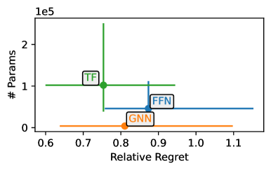
Figure 4: Scatterplot of encoder parameter size and downstream classifier regret at IPC=10 aggregated over datasets and classifiers. The dots represent the median values, and the error bars span the 25% and 75% percentile, respectively. Note that the encoder sizes for both SFT and base versions are the same for each dataset.

With this in mind, we examine the performance difference when training on the distilled data in the latent space or decoding to the original space before training the downstream classifier (using $\tilde{R}$ or $R$ from Algorithm 2). Figure˜3 shows that training on the dataset in the latent space improves the downstream performance for all distillation pipelines – in fact, it is the best performer for almost every instance over classifiers and distillation methods. The change in performance is more apparent in KNN (40.92-65.40%), Logistic Regression (33.75-67.29%) and MLP (33.93-96.38%), while XGBoost shows a more subtle change (7.28-19.20%). This leads us to conclude that distillation methods benefit the most when both distilling and downstream training in on the latent representations. It is also worth noting that decoding the distilled data from the latent space (Rec.) is also beneficial compared to random sampling in many cases.

How do different encoders compare?

Having observed that using the latent space is beneficial, we now seek to identify which encoder architecture leads to the best performance. Table˜1 shows the average rank of distillation pipelines that use the latent space of different encoder architectures. Among the tested architectures and training objectives, the transformer architecture with supervised fine-tuning leads to the best downstream performance. We find that adding supervised fine-tuning improves the downstream performance of all encoders in general.

Another important aspect of data distillation is to improve downstream classifier efficiency providing a lightweight proxy. Thus, it is important to examine the resources required in the distillation pipeline. Specifically, one aspect of our distillation pipelines that can add an additional cost is the encoder. In settings that require the data to be projected into latent space at inference time, the encoder can be considered part of the distilled data. Figure˜4 shows the parameter size of the different encoder architectures vs. the downstream classifier regret scores. As noted before, the transformer architecture leads to the best downstream performance. However, it is worth noting that GNN architecture has the smallest overall parameter size while providing the second-best performance. Further discussion on the parameter size analysis of each encoder architecture can be found in section˜A.3.

Table 2: Relative regret of pipelines that use different combinations of distill methods and encoders at IPC=10, aggregated over classifiers. The best value for each column is marked with bold, and the second best is marked with underline. The best in each distillation method group is marked with italics. On average, $k$-means with SFT transformer shows the best performance, but agglomerative clustering also shows comparable performance.

Distill Method	Encoder	Regret
		Min	Q1	Mean	Median	Q3	Max
KM	TF*	-14.4491	0.0733	-0.0464	0.4056	0.7379	1.1773
	FFN*	-11.9912	0.2039	0.1382	0.6035	0.8389	1.5368
	GNN*	-12.1045	0.0973	0.1054	0.5047	0.7887	1.0494
AG	TF*	-15.3965	0.0810	0.0187	0.4135	0.6507	1.4982
	FFN*	-10.1288	0.2483	0.3695	0.6230	0.8823	4.1191
	GNN*	-13.1881	0.1397	0.2245	0.4793	0.7595	4.4801
KIP	TF*	-4.1619	0.5226	1.1124	0.9415	1.2966	11.1034
	FFN*	-5.3973	0.8053	1.6363	1.2502	1.6434	16.4137
	GNN*	-1.4649	0.7403	1.1957	1.0136	1.3329	10.5175
GM	TF*	-3.8002	0.4105	0.7273	0.7952	1.0564	4.9450
	FFN*	-4.3269	0.5975	1.2660	0.9938	1.3827	16.5044
	GNN*	-1.4776	0.4626	0.8073	0.8457	0.9779	8.4566

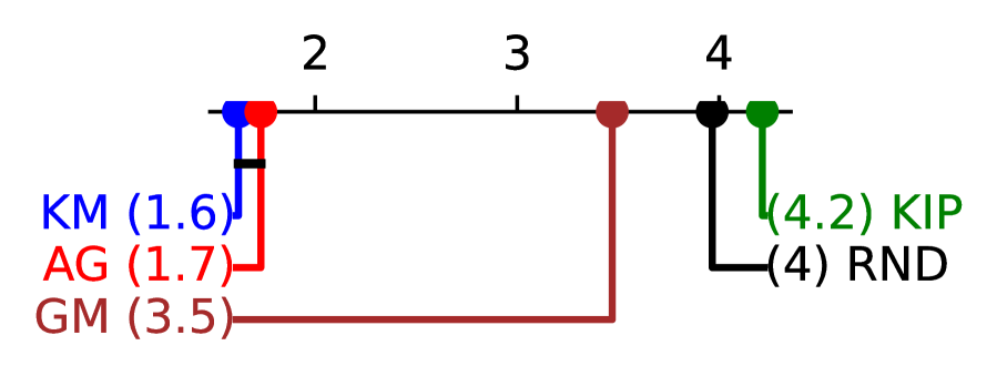
(a) IPC=10

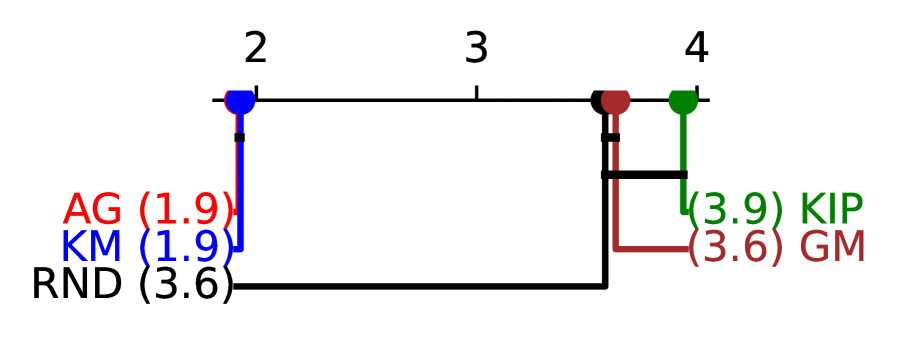
(b) IPC=50

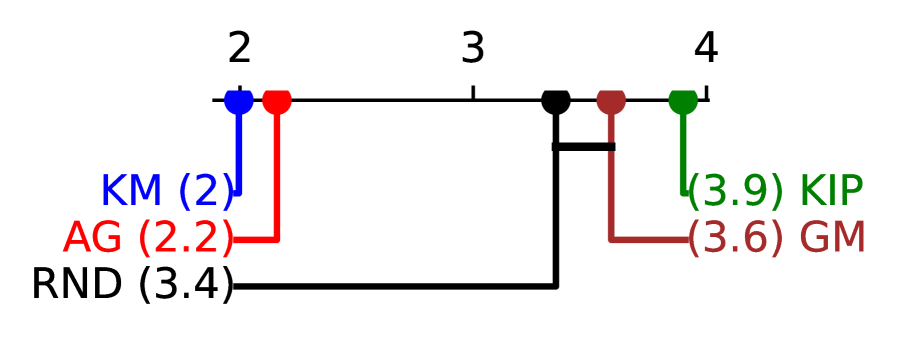
(c) IPC=100

Figure 5: Critical difference plot comparing ranks of distillation methods across datasets, encoders, and classifiers per IPC value. The x-axis denotes the average rank, and a black horizontal line connects groups of methods that are not significantly different in the rank distribution. $k$-means and agglomerative are indistinguishable from each other in $\text{IPC}\in\{10,50\}$, but $k$-means gains an edge in IPC=100.

Which distillation method leads to the best downstream performance?

We now compare the most critical piece of the distillation pipeline – the distillation method.We wish to understand which method leads to the best downstream performance across datasets, encoders, and classifier configurations. To evaluate, we perform a Wilcoxon signed-rank test to identify groups that stand out from the rest, as shown in fig.˜5. The results show that clustering-based methods ($k$-means, agglomerative) show the strongest performance across datasets and encoder configurations, consistently placing in the top two ranks. While both methods show similar performance, we find that $k$-means starts to outperform agglomerative as the IPC increases.

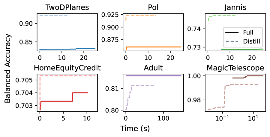
(a) Logistic Regression

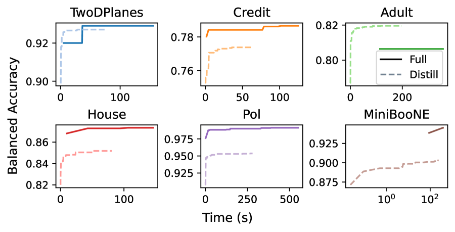
(b) XGBoost

Figure 6: Comparison of HPO validation performance vs. runtime when using full and distilled data. To better visualize the performance difference, we truncate the plot for the full data run at twice the runtime of the entire distilled run.

Table 3: The best performers of each dataset are classifiers ranked by their appearance count at the top $3$ of each comparison at IPC=10. $k$-means stands out as the strongest performer in combination with a supervised-fine-tuned transformer encoder.

Count	Encoder	D.M.	Output
67	TF*	KM	Enc.
63	GNN*	KM	Enc.
61	GNN*	AG	Enc.
61	TF*	AG	Enc.
42	FFN*	KM	Enc.

Which combination leads to best performance?

Our previous analysis has revealed that transformer encoders with SFT and clustering-based distillation methods perform best in their respective comparisons. Now, we aim to identify which combination of encoder and distillation method leads to the best downstream performance. We approach this question by examining the detailed statistics behind the combinations’ performance and the top performers of each dataset, classifier, and $n$ combinations. Table˜2 shows detailed statistics about each distill method and encoder combination, while table˜3 shows the count of the top 5 distillation pipelines that placed in the top 10 by performance in each comparison group. In line with our previous findings, the results show that $k$-means clustering with supervised-fine-tuned transformer encoder leads to the best overall performance. All of the top performers are clustering-based methods, and all of them use the latent space, again confirming that using the latent representation from the encoder greatly benefits distillation methods. In addition, the GNN encoder shows a comparative performance to that of the transformer encoder. This is especially noteworthy, considering that GNN has the smallest parameter size among the encoder architectures.

We additionally run a smaller-scale HPO experiment to consider a use case for distilled data, as seen in  fig.˜6. Specifically, we consider a case where the validation and testing data is sampled from the original data, and the classifier is trained on either the full or distilled data. In general, we note that training on the distilled data gives comparable performance to training on the full data in a fraction of the time, consuming on average 21.84% of the runtime and reaching 98.37% of the performance.

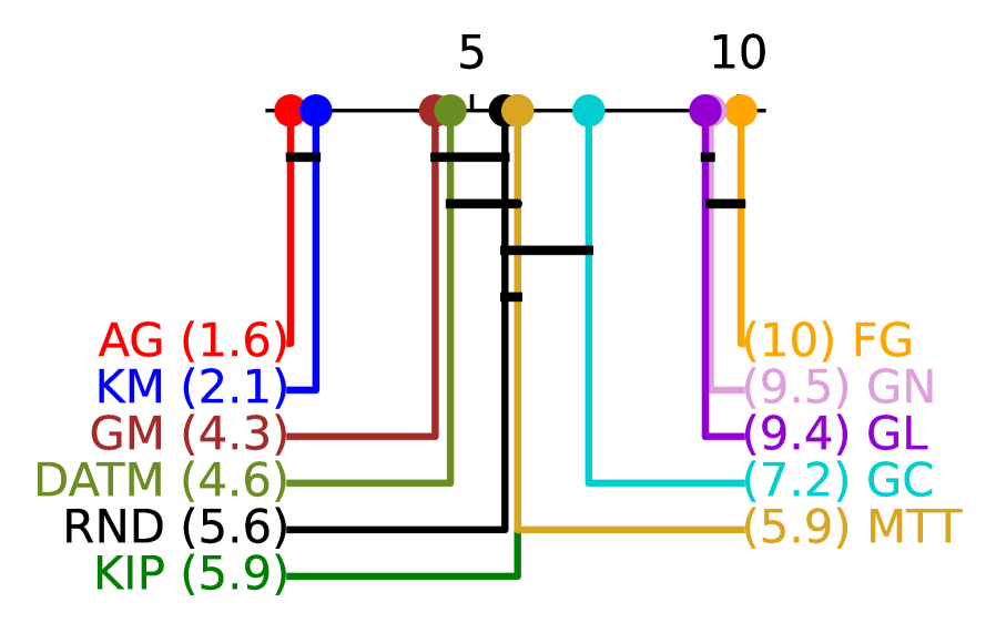
(a) IPC=10

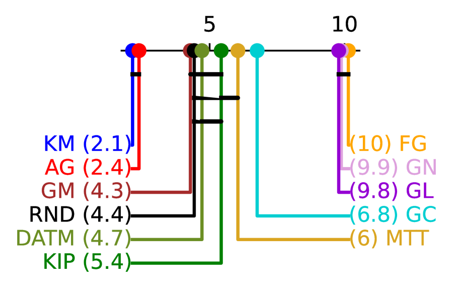
(b) IPC=50

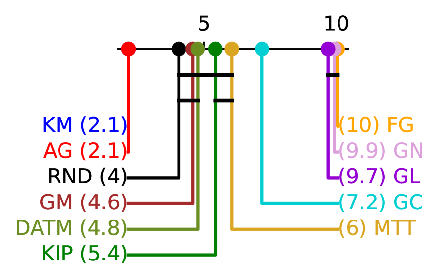
(c) IPC=100

Figure 7: Critical difference plot comparing ranks of distillation methods across datasets per IPC value when applied with TF-SFT encoder for XGBoost classifier with additional baselines The x-axis denotes the average rank, and a black horizontal line connects groups of methods that are not significantly different in the rank distribution. $k$-means and agglomerative are indistinguishable from each other in $\text{IPC}\in\{10,50\}$, but $k$-means gains an edge in IPC=100. (FG: Forgetting, GN: GraNd, GL: Glister, GC: Graph Cut)

How do more recent data distillation methods compare?

We conduct a further comparison of more recent distillation methods against the methods compared in section˜4 to verify whether these methods will show superior performance. Specifically, we incorporate four representative NN-based coreset selection methods examined in DeepCore Guo et al. (2022) – Forgetting Toneva et al. (2018), GraNd Paul et al. (2021), Glister Killamsetty et al. (2021), Graph Cut Iyer & Bilmes (2013)) and MTT Cazenavette et al. (2022) and DATM Guo et al. (2023). Figure˜7 shows the updated critifcal different comparing the additional methods in the best-performing setting. The raw regret scores can be found in table˜18 of Appendix section˜D.1. Consistent to our previous findings, we find that more recent distillation methods that rely on NNs do not fair well on non-differentiable downstream classifier (XGBoost), and that clustering methods still show dominance. It is also interesting to note that GM shows superior performance to MTT and DATM, suggesting that the latter two methods may actually be overfitting to the teacher network’s architecture.

Does distillation preserve feature correlation?

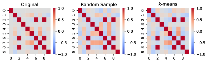
Figure 8: Feature correlation of the original, randomly sampled, and $k$-means distilled version of the Credit dataset@IPC=100.

We further investigate the presevation of feature correlation in the distilled data. Figure˜8 shows th feature correlation heatmaps for each version of the dataset. While the randomly sampled data also preserves most of the correlation, we observe that the dataset distilled with $k$-means is more similar (e.g. interaction between features 3 and 7 of Credit dataset) to the original dataset. We also observe this trend for other datasets, which can be seen in Figure˜18.

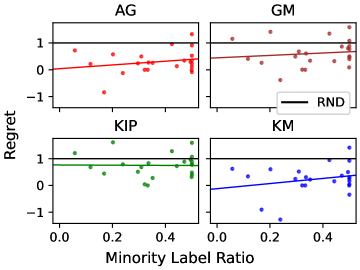
Figure 9: Average median relative regret of distillation methods aggregated over downstream classifiers and encoders at IPC=10 with a least-squares linear regression. Compared to KIP and GM, $k$-means and agglomerative show much stronger performance in imbalanced data.

How does class imbalance affect performance?

Finally, we examine the downstream performance of classifiers with respect to the label balance, or the imbalance, of the original dataset, shown fig.˜9. Compared to other methods, including random sampling, clustering-based methods show impressive strength when distilling datasets with high label imbalance, highlighting their robustness under challenging data distributions. One possible explanation behind this phenomenon is that while NN-based distillation methods may prioritize the majority class due to the imbalance, the clustering methods are forced to place equal emphasis on all classes, preventing an overfitting on the majority class.

5 Discussion

This work introduced a tabular data distillation pipeline and evaluated it extensively leveraging various distillation methods, with a focus on supporting both non-NN and NN ML classifiers. We introduce a novel framework, TDColER, that leverages latent representation of tabular data in distillation, and evaluate it thoroughly in our benchmark, TDBench, which included 23 datasets, 11 distillation algorithms, 3 autoencoder architectures, and 7 downstream classifiers, resulting in over 226,890 distilled datasets and 548,880 downstream classifier instances. Our results show that TDColER can induce superior performance in distillation methods on tabular data, improving the quality by 0.5-143%. We also show that $k$-means clustering and transformer autoencoder are a particularly strong combination for tabular data distillation. We hope that this work will serve as a starting point for future research in tabular data distillation and plan to extend this benchmark further to incorporate new distillation pipelines.

Appendix A Appendix

A.1 Datasets

Table 4: Dataset name and OpenML Vanschoren et al. (2013) url

Dataset Name	Dataset URL
adult	https://api.openml.org/d/1590
Amazon_employee_access	https://api.openml.org/d/4135
Bank_marketing_data_set_UCI	https://api.openml.org/d/44234
credit	https://api.openml.org/d/45027
default-of-credit-card-clients	https://api.openml.org/d/45020
Diabetes130US	https://api.openml.org/d/45022
electrcity	https://api.openml.org/d/151
elevators	https://api.openml.org/d/846
higgs	https://api.openml.org/d/23512
hcdr	https://api.openml.org/d/45071
house_16H	https://api.openml.org/d/821
jannis	https://api.openml.org/d/45021
law-school-admission-bianry	https://api.openml.org/d/43890
MagicTelescope	https://api.openml.org/d/1120
Medical-Appointment-No-Shows	https://api.openml.org/d/43439
MiniBooNE	https://api.openml.org/d/44088
numerai28.6	https://api.openml.org/d/23517
nursery	https://api.openml.org/d/959
PhishingWebsites	https://api.openml.org/d/4534
pol	https://api.openml.org/d/722
road-safety	https://api.openml.org/d/44161
Click_prediction_small	https://api.openml.org/d/1220
2dplanes	https://api.openml.org/d/727

Table 5: Metadata of each dataset seen in table˜4

Dataset	# Instances	# Features	# Cont.	# Cat.	# Class 0	# Class 1
2dplanes	40,768	10	10	0	20,420	20,348
Amazon_employee_access	32,769	9	8	1	1,897	30,872
Bank_marketing_data_set_UCI	45,211	16	7	9	39,922	5,289
Click_prediction_small	39,948	11	11	0	33,220	6,728
Diabetes130US	71,090	7	7	0	35,545	35,545
MagicTelescope	19,020	11	11	0	12,332	6,688
Medical-Appointment-No-Shows	110,527	13	10	3	88,208	22,319
MiniBooNE	72,998	50	50	0	36,499	36,499
PhishingWebsites	11,055	30	0	30	4,898	6,157
adult	48,842	14	6	8	37,155	11,687
credit	16,714	10	10	0	8,357	8,357
default-of-credit-card-clients	13,272	20	20	0	6,636	6,636
electrcity	45,312	8	7	1	26,075	19,237
elevators	16,599	18	18	0	5,130	11,469
hcdr	10,000	22	22	0	5,000	5,000
higgs	98,050	28	28	0	46,223	51,827
house_16H	22,784	16	16	0	6,744	16,040
jannis	57,580	54	54	0	28,790	28,790
law-school-admission-bianry	20,800	11	6	5	6,694	14,106
numerai28.6	96,320	21	21	0	47,662	48,658
nursery	12,960	8	0	8	8,640	4,320
pol	15,000	48	48	0	5,041	9,959
road-safety	111,762	32	29	3	55,881	55,881

Tables˜4 and 5 show the information about datasets used in our experiments along with their OpenML Vanschoren et al. (2013) URLs.

A.2 Hyperparameter optimization for encoders

Table 6: Hyperparameters tested for FFN encoder.

Hyperparameter	Values
d_hidden	$(100,200)$
n_hidden	$[1,4]$
dropout	$(0,0.2,0.4)$
d_embedding	$(10,20,50,100,200)$
use_embedding	$($True,False$)$
learning_rate	$10^{[-3,-1]}$
weight_decay	$10^{[-4,-1]}$
lr_scheduler	$($None, Plateau, Cosine$)$

Table 7: Hyperparameters tested for GNN encoder.

Hyperparameter	Values
graph_layer	$($graphsage, gcn, gat$)$
graph_aggr	$($mean, softmax$)$
n_graph	$[1,15]$
edge_direction	$($bidirectional, multipass$)$
edge_dropout	$(0,0.2,0.4)$
learning_rate	$10^{[-3,-1]}$
weight_decay	$10^{[-4,-1]}$
lr_scheduler	$($None, Plateau, Cosine$)$

Table 8: Hyperparameters tested for TF autoencoder.

Hyperparameter	Values
n_blocks	$[1,10]$
n_attention_heads	$2^{[1,4]}$
d_qkv	$2^{[0,7]}$
layer_norm_eps	$10^{[-5,-1]}$
d_mlp	$2^{[7,11]}$
d_mlp_hidden	$(100,200)$
n_mlp_hidden	$[1,4]$
dropout	$[0,0.4]$
learning_rate	$10^{[-3,-1]}$
weight_decay	$10^{[-4,-1]}$
lr_scheduler	$($None, Plateau, Cosine$)$

Table 9: Hyperparameters tested for decoders. The decoder architecture is kept the same for all encoders and optimized individually.

Hyperparameter	Values
d_hidden	$(100,200)$
n_hidden	$[1,4]$
learning_rate	$10^{[-3,-1]}$
weight_decay	$10^{[-4,-1]}$
lr_scheduler	$($None, Plateau, Cosine$)$

Table 10: Hyperparameters tested for classifier head in SFT.

Hyperparameter	Values
d_hidden	$\{100,200\}$
n_hidden	$[1,3]$
dropout	$\{0,0.2,0.4\}$
alpha	$\{0.3,0.5,0.7\}$
learning_rate	$10^{[-3,-1]}$
weight_decay	$10^{[-4,-1]}$
lr_scheduler	$($None, Plateau, Cosine$)$

Tables˜6, 7, 8, 9 and 10 show the hyperparameters considered for different modules of the autoencoders. We use $\{x,y,z\}$ to denote a set of variables and $[a,b]$ to denote an inclusive range of values. We conduct HPO for each autoencoder + dataset pair using an implementation of hyperopt Bergstra et al. (2015) from Ray Tune Liaw et al. (2018) with a maximum of 500 samples for each HPO run. As noted in section˜2.1, we first train the vanilla autoencoders for each dataset using the encoder hyperparameters seen in tables˜6, 7 and 8 and decoder parameters seen in table˜9. Once the vanilla autoencoders are trained, we then conduct an additional fine-tuning with a classifier head with hyperperameters seen in table˜10 where $\alpha$ is used to balance the objective functions of the decoder and classifier heads.

A.3 Discussion on parameter size of autoencoders

Here we expand on our parameter size of the encoder architectures of the autoencoders. This is worth noting because if the distilled data is in the latent space, the encoder module is required to project any new data to the same space. Thus, the encoder is considered to be a part of the distilled output.

We can characterize the parameter size of each encoder architecture given a $D$-dimensional binarized dataset with $c$ categorical features and $r$ continuous features that is projected to a $d$-dimensional latent space.

FFN. We used an FFN architecture with an $M$-dimensional embedding layer followed by $H$ hidden layers that receive and output $W$-dimensional vectors. The parameter size of such an FFN is as follows:

$$O(DM+(c+r)MW+HW^{2}+Wd)$$ (5)

The column embeddings are of size $O(DM)$, the input layer maps the concatenated $(c+r)M$-dimensional vector to hidden layer dimension $W$ with $(c+r)MW$ size. The hidden layers are of sizes $O(W^{2})$ each for $H$ hidden layers. The output layer maps the $W$-dimensional hidden layer output to the desired $d$-dimensions.

GNN. We use a GNN encoder with $H$ consecutive layers. The dimension of the vectors passed between the graph layers are fixed to $d$, meaning that $M=d$. Thus, each graph layer maintains a $d$ by $d$ matrix to handle a $d$-dimensional input vector and output a $d$-dimensional vector.

$$O(Dd+Hd^{2})$$ (6)

The column embeddings are of size $O(Dd)$ since $M=d$. Each of the $H$ GNN layers is of size $O(d^{2})$.

Transformer. We consider an implementation of a transformer autoencoder inspired by the architecture of FT-Transformer Gorishniy et al. (2021). The encoder has an $M$-dimensional embedding layer followed $H$ transformer blocks. Each transformer block takes in a sequence of $M$-dimensional embeddings and oututs a single $d$-dimensional vector. The block is composed of a multihead-attention module with $m$ heads and a FFN module to project the attention scores back to the input space. We modify the architecture seen in (Gorishniy et al., 2021) by allowing the dimension of the attention head to be configurable – i.e. instead of using $M/m$ as the dimension of a single attention head, we allow the module to compute the attention in $d_{qkv}$. This choice is motivated by the fact that our encoders were trained with a latent size of $16$, which may not be wide enough for the TF encoder. We then project the resulting embedding in $d_{qkv}m$-dimension back to $M$-dimensionals with $W_{o}$. Thus, each of $W_{q}$, $W_{k}$, $W_{v}$ and $W_{o}$ has $d_{qkv}mM$ parameters. The MHA module is then followed by an FFN module which takes a $M$-dimensional vector and projects it back to $M$-dimensions with a $W$-dimensional hidden layer.

$$O(H(4d_{qkv}Mm+2MW))$$ (7)

A.4 Autoencoder implementation details

[width=]./tikz/ffn

Figure 10: FFN encoder.

[width=]./tikz/gnn

Figure 11: GNN encoder.

[width=0.8]./tikz/mha

Figure 12: Modified MHA component.

[width=0.8]./tikz/tfblock

Figure 13: TF encoder block.

A.4.1 Optimization function

For the decoder $\psi:\mathbb{R}^{d}\to\mathbb{R}^{D}$, we consider a multi-layered fully-connected feed-forward network. Given the encoder $\phi$ and the decoder $\psi$, we use a group-wise softmax operator $\sigma$ to map the output of the decoder to a per-input-feature probability simplex: given an initial binary vector $b\in\{0,1\}^{D}$ constituting per-input-feature one-hot encodings $b^{i}$ (that is $b=[b^{1}\oplus\ldots\oplus b^{c+r}]$), and a decoder output $B\in\mathbb{R}^{D}$ with per-input-feature constituents $B^{i}$ (that is $B=[B^{1}\oplus\ldots\oplus B^{c+r}]$, we apply the softmax operation to each per-input-feature constituent to get $\hat{b}=[\hat{b}^{1}\oplus\ldots\oplus\hat{b}^{c+r}]\in[0,1]^{D}$, where $\hat{b}^{i}=\textsf{softmax}(B^{i})$. We utilize the following per-sample reconstruction loss:

$$\ell(b,\hat{b})=\tfrac{1}{c+r}\textstyle\sum_{i=1}^{c+r}\frac{1}{\log_{2}|b^{i}|}\textsf{CE}(b^{i},\hat{b}^{i}),$$ (8)

where CE is the standard cross-entropy loss between a one-hot vector and a softmax output, and $|b^{i}|$ is the length of the $i$-th constituent one-hot encoding in $b$, corresponding to the number of categories (or bins) in the $i$-th categorical (or numerical) feature. This loss is a weighted average of the per-input-feature cross-entropy loss, with weights $(\nicefrac{{1}}{{\log_{2}|b^{i}|}})$ to normalize the loss across all features with varying number of categories or bins.

The encoder and decoder are then learned by optimizing the following unsupervised loss:

$$\mathcal{L}_{R}(\phi,\psi)=\tfrac{1}{N}\textstyle\sum_{(x,y)\in S}\ell\left(P(x),\sigma(\psi(\phi(P(x))))\right),$$ (9)

where $P$ is the data homogenizer, and $\sigma$ is the aforementioned group-wise softmax operator. Learning the latent representation in such an unsupervised manner makes this distillation pipeline agnostic to the choice of downstream model. Another advantage of this choice is that the decoder allows us to map the distilled artificial samples in the latent space to the original features, which might be necessary in some applications (for interpretability reasons).

A.4.2 Supervised latent space fine-tuning

Given the already learned encoder and decoder, we consider a supervised fine-tuning (FT) step where we utilize a classifier $f:\mathbb{R}^{d}\to Y$ that utilizes the latent representation. The classifier is learned, and the encoder and decoder are fine-tuned by minimizing the following loss to ensure that the latent space is quite predictive while the reconstruction loss stays low:

$$\mathcal{L}_{R}(\phi,\psi)+\textstyle\frac{\alpha}{N}\sum_{(x,y)\in S}\textsf{CE}(y,f(\phi(P(x)))),$$ (10)

where $\alpha>0$ is penalty parameter to balance the two losses, and CE is the cross-entropy loss. We consider multi-layer FFN architecture as the classifier $f$.

A.4.3 Encoder architectures

Fully-connected feed-forward network (FFN). This encoder first selects the column embeddings corresponding to nonzero entries in the binary representation $b$, concatenates them to get a $(c+r)M$-dimensional dense vectors (recall that $b$ will only have $c+r$ nonzeros out of the $D$ dimensions), and inputs them to a fully-connected feed-forward network $\mu:\mathbb{R}^{(c+r)M}\to\mathbb{R}^{d}$. The encoder $\phi:\{0,1\}^{D}\to\mathbb{R}^{d}$ can be written as:

$$z=\phi(b)=\mu(\oplus([w_{i},i\in\{1,\ldots,D\}:b[i]=1])),$$ (11)

where $b[i]$ is the $i$-th entry of the $D$-dimensional vector, and $\oplus$ is the concatenation operator. The FFN $\mu$ and the column embeddings $\{w_{i},i\in\{1,\ldots,D\}\}$ constitute the parameters of the encoder $\phi$. For a FFN with $H$ hidden layers, each of width $W$, the total number of parameters in this encoder is $O(DM+(c+r)MW+HW^{2}+Wd)$. Figure˜10 shows a simplified architecture of the FFN encoder.

Graph neural network (GNN) encoder. We also consider a more recent encoder for tabular data proposed in Wu et al. (2021). A bipartite graph is constructed between the column embeddings $\{w_{i},i\in\{1,\ldots,D\}\}$ and the (zero-initialized) row (sample) embeddings $\{z_{j}\in\mathbb{R}^{d},j\in\{1,\ldots,N\}\}$, with a bidirectional edge between $w_{i}$ and $z_{j}$ if the $b_{j}[i]=1$, where $b_{j}\in\{0,1\}^{D}$ is the binary representation of the $j$-th sample. Given the (learned) column embeddings, the row embeddings are obtained via multiple rounds of message passing through multiple GNN layers. This can be written as:

$$\begin{split}&z_{j}^{h}=\mu_{h}(z_{j}^{h-1},\textsf{Agg}(w_{i}^{h-1},i\in\mathcal{N}_{j})),\\ &w_{i}^{h}=\mu_{h}(w_{i}^{h-1},\textsf{Agg}(z_{j}^{h},j\in\mathcal{N}_{i})),\end{split}$$ (12)

where $\mu_{h}$ is the $h$-th GNN layer, Agg is an aggregation, $\mathcal{N}_{i}$ (or $\mathcal{N}_{j}$) is the neighbor set of the $i$-th column embedding (or $j$-th row embedding). We set the initial $z_{j}^{0}=0$ (zero-initialized row embeddings), $w_{i}^{0}=w_{i}$, and utilize $z_{j}^{H}$ as the latent representation for distillation after $H$ GNN layers. While Wu et al. (2021) only considered Graph Convolutional Networks Kipf & Welling (2016) as GNN modules, we extend it to GraphSage Hamilton et al. (2017) and Graph Attention Networks Veličković et al. (2018). An important aspect of the GNN encoder is that the desired row embedding size $d$ must match the column embedding size $M$, thus $d=M$. With $H$ GNN layers, the total number of parameters in this encoder is usually $O(Dd+Hd^{2})$, which can be significantly smaller than the FFN encoder with moderately sized FFN (large enough $M$, $W$). Figure˜11 shows the graph formulation (left) and the GNN encoder architeture (right).

Transformer encoder. Finally, we consider a transformer-based autoencoder inspired by the architecture of FT-Transformer Gorishniy et al. (2021). This encoder uses the same embedding layer as the FFN encoder, which is then followed by transformer blocks. We learn an additional $cls$ embedding, which is placed before all other tokens in every sequence. Each block takes in a sequence (one row) of $d$ embeddings, and is composed of a multihead-attention (MHA) module and a feed-forward network (FFN) module.

For a MHA module with $m$ attention heads, we modify the architecture seen in (Gorishniy et al., 2021) by allowing the dimension of the attention head to be separately configurable – i.e. instead of using $d/m$ as the dimension of a single attention head, we allow the module to compute the attention in $d_{qkv}$. This choice is motivated by the fact that our encoders were trained with a latent size of $16$, which may not be wide enough for the TF encoder. We then project the resulting embedding in $d_{qkv}m$-dimension back to $d$-dimension with $W_{o}$. For an input $w_{i}$ at the $i$th transformer block, the computation for the MHA module is as follows:

$$a_{i}=W_{o}^{i}(\textsf{softmax}(\frac{W_{q}^{i}(w_{i})W_{k}^{i}(w_{i})}{\sqrt{d_{qkv}}})W_{v}^{i}(w_{i}))$$ (13)

The resulting attention score $a_{i}$ is then added with the original embedding and passed through an FFN module. Similarly to Gorishniy et al. (2021), the [cls] embedding is used as the final output of the encoder. Figure˜12 shows our modified MHA component, and fig.˜13 shows the TF encoder block.

A.5 Distill Methods

A.5.1 Choice of Distill Methods (KIP, GM)

The clustering-based distillation schemes and KIP are not explicitly tied to a specific model and thus satisfy our desiderata of model-agnosticity. In contrast, the Gradient Matching or GM distillation scheme heavily relies on the choice of the backbone model $M_{\theta}$ (as well as the learning algorithm parameters such as the learning rate), and there is no guarantee that the distilled samples $R$ would be useful for any other model. Thus, this scheme is not model-agnostic. However, we consider GM to be representative of the model-specific distillation schemes for the sake of completeness of our evaluations. For our table distillation, we choose $M_{\theta}$ to be a multi-layered perceptron with a single hidden layer. This will pose a mismatch when we evaluate the quality of the distilled data $R$ on standard tabular models such as decision tree ensembles and nearest-neighbor models, highlighting the need for model-agnosticity in tabular data distillation.

A.5.2 Distill Method Implementaion

Table 11: Parameters of distillation methods.

Method	Hyperparameter	Value	Description
Common	distill space	-	Whether to use the encoder latent space or the raw binary representation.
	use_closest*	-	Whether to use median points instead of the euclidean center. Only applicable to clustering methods.
	output_space†	-	Whether to keep the encoder latent/ decode or use the raw binary space. The binary space is only applicable to clustering methods when use_closest is set to True.
	random_seed‡	-	Random seed for distillation algorithm. Not applicable to agglomerative.
KIP	n_epochs	$1000$	Number of epochs to train the distilled data.
	mlp_dim	$1024$	Width of the neural network to compute the NTK of.
GM	n_epochs	$500$	Number of epochs to train the distilled data.
	mlp_dim	$1024$	Size of the hidden layer of the target model.
	n_layers	$2$	Number of hidden layers in the target model.
	lr_mlp	$0.01$	Learning rate for the target model.
	lr_data	$0.1$	Learning rate for the distilled data.
	mom_data	$0.5$	Momentum for distilled data.

$k$-means

We use the sklearn.cluster.KMeans from Pedregosa et al. (2011) with the n_init set to "auto".

Agglomerative

We use sklearn.cluster.AgglomerativeClustering from Pedregosa et al. (2011) with the linkage set to "ward". Because agglomerative clustering does not have a “centroid”, we manually calculate a euclidean centroid for each cluster by using sklearn.neighbors.NearestCentroid to compute the centroid or the closest real point.

KIP

We use the implementation provided by Nguyen et al. (2021) available at https://github.com/google-research/google-research/tree/master/kip.

GM

We use the implementation provided by Zhao et al. (2021) available at https://github.com/VICO-UoE/DatasetCondensation.

Table˜11 shows the parameters available for each distillation methods. The common parameters are used for every algorithm, with the exceptions marked on the right-most column. The method-specific parameters for KIP and GM are for the original algorithms as proposed in Nguyen et al. (2021); Zhao et al. (2021).

A.6 Downstream Classifier Hyperparameters

Table 12: Hyperparameters of downstream classifiers.

Classifier	Hyperparameter	Value
FT-Transformer	d_token	$128$
	n_blocks	$2$
	attention_n_heads	$8$
	attention_dropout	$0.15$
	ffn_d_hidden_multiplier	$1.25$
	ffn_dropout	$0.05$
	residual_dropout	$0$
	learning_rate	$10^{-4}$
	weight_decay	$10^{-5}$
	early_stopping	True
Naive Bayes	var_smoothing	$10^{-9}$
$K$-Nearest-Neighbors	n_neighbors	$5$
	leaf_size	$30$
	p	$2$
Logistic Regression	penalty	l2
	tol	$10^{-4}$
	C	$1$
	solver	lbfgs
MLP	d_hidden	$100$
	n_hidden	$1$
	learning_rate	$10^{-4}$
	early_stopping	True
ResNet	n_blocks	$4$
	d_block	$128$
	d_hidden_multiplier	$1.25$
	dropout	$0.2$
	learning_rate	$0.0001$
	weight_decay	$0.00001$
	early_stopping	True
	patience	$16$

Table˜12 shows the hyperparameters used for each downstream classifier. We use scikit-learn Pedregosa et al. (2011)’s implementation of Naive Bayes, $K$-Nearest-Neighbors, Logistic Regression, and MLP, and Gorishniy et al. (2021)’s implementation of FT-Transformer and ResNet.

A.7 ResNet and FT-Transformer performance

Table 13: Average train/test times and test performance comparison for all downstream classifiers.

Classifier	Train Time	Test Time	Test Perf.
FTTransformer	281.3431	0.17934	0.7879
NB	0.0030	0.00232	0.6624
KNN	0.0007	0.54309	0.7474
LR	0.4901	0.00646	0.7709
MLP	2.4444	0.00554	0.7826
ResNet	154.9824	0.08508	0.7833
XGB	11.4055	0.01439	0.8180

We test ResNet and FT-Transformer for 5 datasets. We found that even with early stopping, the two classifiers take significantly longer to train given the same computing resources. On average, we find that ResNet takes around 10 times longer to finish training, while FT-Transformer takes around 28 times when compared to XGBoost. We also find that the performance of resnet and FT-Transformer does not stand out – in fact, the average test performance when trained on the full dataset shows that both ResNet and FTTransformer show a similar performance to MLP, and are outperformed by XGBoost.

A.8 Determining the best overall performance

We describe the best overall pipeline in section˜4 and table˜3. Here, we provide a more detailed explanation of how we determined the best overall pipeline. The runs are grouped by their classifier, dataset and distill size $n$. Similar to other parts of analysis, the grouping is done in order to ensure that the comparisons are fair. In this instance, we are interested in only the pipeline components that lead to the best classifier performance, regardless of the exact classifier kind. Thus, we group every run by their non-pipeline-specific parameters, which are the classifier, dataset and distill size $n$. In each group, we then count the instances the pipeline places on the top 3 in terms of the regret score and sum up the counts for each pipeline.

Following the previous findings, table˜3 shows that $k$-means based methods have the best performance, placing in the top 3 with all SFT encoder variants. Surprisingly, we also find pipelines that use KIP and GM as the 4th and 5th best performers. While we were not able to determine any specific conditions that cause KIP and GM to place on top, this result shows that there are exist some conditions which leads the pipelines using gradient-based methods (KIP, GM) to be the top performer. On the other hand, the consistent rank placement of pipelines that use the autoencoder latent space shows that fine-tuned autoencoders can indeed boost the performance of distillation methods significantly.

Appendix B Additional Analysis

B.1 Full results of distillation methods by downstream classifiers

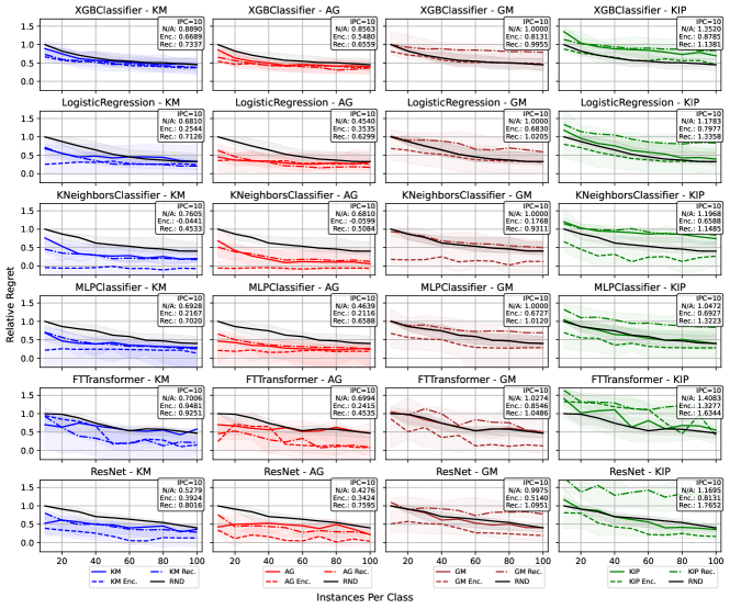
Figure 14: Full results of distillation methods by downstream classifiers.

B.2 Effect of column embedding scheme on downstream performance

Table 14: A comparison of relative regret scores of distillation pipelines that use the encoded space of autoencoders trained with different column embeddings, tested on 5 datasets (Adult, Amazon Employee Access, Credit, House, Phishing Websites). The center value shows the median relative regret, and smaller values on each side refers to the first and third quantile, respectively. In general, PLE embeddings show the strongest performance. However, it is worth noting that PLE embeddings are not applicable to GNN encoders, and that binary embeddings also show superior performance to scaled embeddings.

Col. Emb.	KM	AG	GM	KIP
Binary	0.1082 0.5645 0.7886	0.0976 0.4633 0.7181	0.5504 0.9038 1.0063	0.6551 0.9254 1.1918
Scaled	0.7214 0.8613 1.0671	0.4908 0.6939 1.0249	1.0092 1.4412 1.8658	1.3304 1.6137 2.2985
PLE	-0.2428 0.1976 0.9305	-0.2698 0.2173 0.6752	-0.0865 0.2747 1.0524	-0.0263 0.7398 1.3923

While column embeddings are standard for categorical columns – each category is represented with a vector, there are various ways of embedding numerical columns: (i) A numerical feature can be binned, and each bin treated as a category with an embedding ${\mathbf{w}}\in\mathbb{R}^{m}$ corresponding to each bin. (ii) With linearly scaled column embeddings, a single column embedding ${\mathbf{w}}\in\mathbb{R}^{m}$ is used for each numerical column, and the column embedding for a particular numerical value $v\in\mathbb{R}$ is obtained by scaling ${\mathbf{w}}$ to $v\cdot{\mathbf{w}}$. (iii) Piecewise linear encoding or PLE (Gorishniy et al., 2022) also bin the numerical feature but use a more sophisticated way of generating the column embeddings for a given numerical value. We considered binned numerical features in the main paper for a couple of reasons: (a) Binned numerical features naturally handle missing values (quite prevalent in tabular data) by maintaining a “missing” bin instead of relying on a heuristic intermediate imputation step; sometimes, the fact that a value is missing is in itself a signal, and heuristic imputation schemes often lose this information. (b) The binned features can be used for all architectures we consider here – FFN, Transformer, and GNN – and using a common embedding scheme allows us to ablate the effect of the different architectures. The other numerical embedding schemes do not apply to GNNs.

To understand the effect of different kinds of column embeddings schemes, we conduct a smaller scale experiment on 5 datasets. Specifically, we compare scaled embeddings as seen in Gorishniy et al. (2021), piecewise linear encoding (PLE) as seen in Gorishniy et al. (2022), against using binary column embeddings where continuous features are binarized by binning, and examine the downstream performance of distillation pipelines that use the latent space of the autoencoders trained with the corresponding column embedding scheme. Table˜14 shows that using the both binary column embeddings and PLE consistently leads to lower regret scores compared to scaled column embeddings. While PLE embeddings show the strongest performance, they are not applicable to the GNN autoencoder architecture. Thus, we conduct most of our experiments using binary column embeddings for a fair comparison across different autoencoder architectures for a fair comparison.

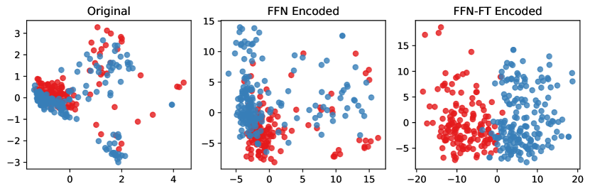
Figure 15: PCA visualization of Phishing Websites dataset.

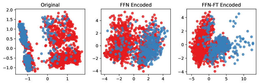
Figure 16: PCA visualization of the Adult dataset.

B.3 Effect of supervised fine-tuning.

Figures˜15 and 16 show the PCA visualizations the adult and tencent CTR datasets in the original, FFN-encoded, FFN-SFT encoded representations. Both figures show that while the distribution inside the vanilla FFN’s latent space does not look significantly different from the original space, adding supervised fine-tuning leads to a clearer separation between different classes.

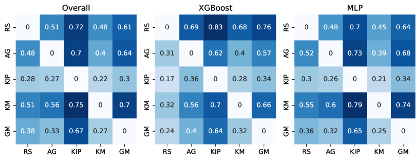
Figure 17: Pairwise comparision of distillation methods. The relative performances of distillation methods under otherwise equal sttings. Rows denote win ratio, columns denote loss ratio.

B.4 Pairwise comparision of distillation methods.

In addition, we compare the downstream classifier performance with every pair of pipelines that use different distillation methods under otherwise equal settings. The left table of fig.˜17 reveals that KIP had the highest tendency to underperform other distillation methods, while k-means had the highest tendency to outperform other distillation methods. This is consistent with our previous findings, where k-means outranked other distillation methods most frequently. In order to gain further insights behind the performance lag of graident-based distillation methods, we conduct a pairwise comparison of the distillation methods for different classifiers as well. The center and right tables of fig.˜17 shows the pairwise comparison of distillation methods for XGBoost and MLP as downstream models. This suggests that gradient-based methods’ underperformance is not solely due to its kernel, but that tabular data itself may pose a unique challenge in distillation that is not seen in image data. It is also worth noting that while the clustering-based approaches had the best overall rank, random sampling proved to be a strong baseline with a near 50% win ratio against them.

Appendix C Documentation of TDBench

The information in this section is also available in a markdown format in the README.md file of the supplementary material.

C.1 Reproducing Results

Every plot and table in the main paper can be reconstructed using the following scripts:

• Q0_experiment_scale.py

• Q1_1_col_embeds.py

• Q1_encoding.py

• Q2_distill_methods.py

• Q3_autoencoders.py

• Q4_1_runtime.py

• Q4_2_get_hpo_dirs.py

• Q4_2_hpo.py

• Q4_combinations.py

• Q5_class_imbal.py

The scripts are organized in order of the question addressed in section˜4 and will be populated in iclr-figures directory. These can be simply ran by calling python SCRIPT_NAME.

The following files are included in the supplementary material and contain all the necessary information for the scripts:

• dataset_stats.csv

• enc_stats.csv

• *data_mode_switch_results.csv

• hpo-measure/

• *mixed_tf_results.csv

• *ple_tf_results.csv

The files marked with an asterisk (*) are not included in the repository, but can be downloaded from this url: https://drive.google.com/drive/folders/1tJ5e1iCvaz-UbxEgpmuCPj-58crgYRJW?usp=share_link

C.2 Description of the workflow

The ## Running the Code section of README.md file discusses the actual commands and available options for running each stage in detail.

The procedure is as follows:

• Train the autoencoder with the desired configuration.

• (Optional) Fine-tune the autoencoder with a classifier head.

• Run distillation methods against specified downstream classifiers.

C.3 Constructing a new pipeline

Changing default parameters

The configurations for this project are managed by hydra and can be modified by adding new files/directories under the ‘config‘ directory.

Adding new datasets

Adding new datasets is as simple as adding a new config/data/datasets/DATASET_NAME.yaml file. Currently, only openml datasets are supported.

Field	Type
dataset_name	string
download_url	string
label	string
n_classes	int
source_type	string

Table 15: Configuration details for datasets

The following flags must be specified for the dataset to be correctly loaded as seen in table˜15.

Adding new preprocessing methods

Field	Type
parse_mode	string
scale_mode	string
bin_strat	string
n_bins	int

Table 16: Configuration details for data preprocessing

The preprocessing is handled by the TabularDataModule object that lives in tabdd/data/tabulardatamodule.py. The preprocessing strategies are identified by a string, and can be configured under config/data/mode. The fields seen in table˜16 must be specified for the preprocessing to work correctly. One can additionally define any type of scale_mode or bin_strat, which will be consumed by the TabularDataModule.

This object is configured with DatasetConfig and DataModeConfig. The DatasetConfig is the configuration for the dataset, and the DataModeConfig is the configuration for the preprocessing method.

It’s TabularDataModule.prepare_data is the method that will parse the data accordingly and save to cache. One can add arbitrary preprocessing methods in this file by adding new flags to DataModeConfig and handling it inside the prepare_data method.

Adding new distillation methods

Field	Type
is_random	string
is_cluster	string
can_use_encoder	string
args	int

Table 17: Configuration details for distillation methods

The distillation methods are identified by a string, which should have a configuration with the same name under config/distill/methods. Once can characterize the method the following fields seen in table˜17.

• is_random: Whether there is randomness in the method. If true, the pipeline will be ran multiple times.

• is_cluster: Whether the method is a clustering method. If true, an option that uses the nearest-to-center method will be included.

• can_use_encoder: Whether the method can be applied in the latent space.

• args: any additional arguments to the actual function.

Once the configuration is created, it will be consumed by load_distilled_data method of tabdd/distill/load_distilled_data.py. This method can then be modified to include the new distillation method.

Adding new encoders

All encoders used in the benchmark are subclasses BaseEncoder from tabdd/models/encoder/base_encoder.py. A simple example of how to implement can be seen in tabdd/models/encoder/mlp_autoencoder.py. The module needs to encoder the following methods: __init__(), encode, decode and forward.

The autoencoders are specified by the configuration files in config/encoder/models/. The class of the encoder is specified by cls, and the hyperparameters are specified by tune_params.

Appendix D Additional Analysis

D.1 Additional Distillation Methods

Table 18: Relative regret of pipelines that use different combinations of distill methods and encoders at IPC=10, aggregated over classifiers. The best value for each column is marked with bold, and the second best is marked with underline. (FG: Forgetting, GN: GraNd, GL: Glister, GC: Graph Cut)

Distill Method	Regret
	Min	Q1	Mean	Median	Q3	Max
Random Sample	1.0000	1.0000	1.0000	1.0000	1.0000	1.0000
KM	0.0597	0.5256	0.6682	0.6654	0.8186	1.1094
AG	0.0000	0.5177	0.6301	0.6036	0.8914	0.9965
KIP	0.6728	0.8483	1.1109	1.0544	1.2523	2.2713
GM	0.4175	0.7707	0.9858	0.9377	1.1461	1.7292
FG	0.8705	1.1400	2.3837	1.4465	1.8731	16.0146
GN	0.7748	1.1498	2.0530	1.3704	2.2624	10.6670
GL	0.8376	1.1000	2.0907	1.3146	1.6823	14.1625
GC	0.6361	0.9077	1.5084	1.1031	1.5998	6.8392
MTT	0.4175	0.7707	1.0340	0.9699	1.2176	2.3026
DATM	0.4175	0.7707	1.0340	0.9699	1.2176	2.3026

D.2 Dataset Feature Correlation

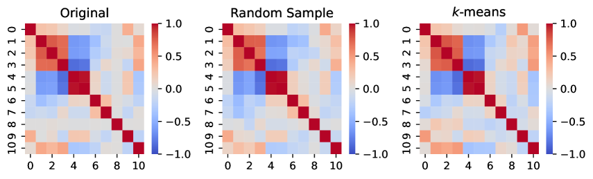
(a) Magic Telescope

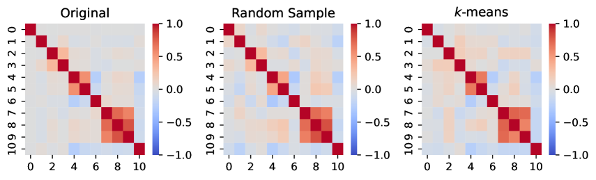
(b) Tencent CTR

Figure 18: A side-by-side comparison of correlation of numerical features in the training data before distillation, after random sampling@IPC=100, and after distillation@ICP=100. While some weaker correlations are not entirely accurately portrayed, the distilled data preserves the stronger correlations remarkably well.

We further investigate the presevation of feature correlation in the distilled data. Figure˜18 shows the change in feature correlation in the original, randomly sampled and distilled with $k$-means in the latent space of TF-SFT in 3 datasets – Credit, Magic Telescope and Tencent CTR.

D.3 Relation to Previous Work

Kang et al. (2024) presented a preliminary abstract on work that explores data distillation for tabular data. The authors utilize an MLP and GNN based autoencoder networks to transform the data to before distilling and show that simple clusetering-based methods can outperform competetive distillation algorithms proposed in computer vision (KIP (Nguyen et al., 2021))

Building upon this work, our work provides a comprehensive analysis of distillation methods on tabular data, and provides a detailed comparison of distillation methods across a wide range of datasets and classifiers. We also provide a detailed analysis of the effect of IPC on the performance of distillation methods, and provide insights into the effect of distillation on the feature correlation of the data.

Below, we provide a detailed comparison of our work with the preliminary abstract presented by Kang et al. (2024):

• We conduct a comprehensive comparison of different binning methods and their effect on downstream performance.

• We test with a transformer-based autoencoder, and show that it outperforms MLP and GNN based autoencoders.

• We additionally consider gradient matching Zhao et al. (2021) as an additional baseline to represent the gradient-based family of distillation methods Cazenavette et al. (2022); Zhao & Bilen (2023); Guo et al. (2023)

• We provide a complete python package, TDBench, that can be used and extended by anyone in the community.

• We explore a realistic use case for data distillation in the context of HPO and show the trade-offs in utility and cost saving.

• We introduce a relative regret metric to compare the performance of different distillation methods across datasets and classifiers.

D.4 Raw balanced Accuracy score

Below is a comparison of the raw balanced accuracy of each distillation pipelines averaged over random iterations. Table˜19 shows a comparison of all 10 distillation methods that were ran with TF-SFT encoder and tested on XGB downstream classifier, and table˜20 shows the performance of the baseline methods when applied without the encoders.  Tables˜21 and 22 show the same comparison that with and without TF-SFT encoder for the 4 baselines methods ($k$-means, aggloermative, KIP, GM) on KNN classifier, and tables˜23 and 24 show the same for MLP classifier.

The last two rows of the tables each denote the number of instances that the pipeline ranked at the top, and the number of times it outperformed random sampling. The results show that random sampling is not a trivial baseline for many methods, and that both clustering methods, AG and KM, show the strongest performance. We also see that adding the encoder to the pipeline significantly increases the downstream performer of all 3 representative models.

angle=90 Dataset AG DATM FG GM GL GN GC KIP KM MTT AD 0.7409$\pm$0.0128 0.7304$\pm$0.0316 0.6779$\pm$0.0458 0.7304$\pm$0.0316 0.5241$\pm$0.0000 0.5241$\pm$0.0000 0.6491$\pm$0.0545 0.7174$\pm$0.0517 0.7425$\pm$0.0220 0.7304$\pm$0.0316 AE 0.5072$\pm$0.0017 0.5233$\pm$0.0250 0.4960$\pm$0.0355 0.5253$\pm$0.0308 0.4950$\pm$0.0086 0.5149$\pm$0.0348 0.5418$\pm$0.0119 0.5107$\pm$0.0228 0.5292$\pm$0.0210 0.5233$\pm$0.0250 BM 0.7519$\pm$0.0258 0.7619$\pm$0.0124 0.6247$\pm$0.0878 0.7619$\pm$0.0124 0.3536$\pm$0.0325 0.5063$\pm$0.0007 0.7204$\pm$0.0387 0.7113$\pm$0.0425 0.7418$\pm$0.0110 0.7619$\pm$0.0124 CR 0.5215$\pm$0.0079 0.5463$\pm$0.0119 0.4606$\pm$0.0078 0.5463$\pm$0.0119 0.5051$\pm$0.0097 0.4990$\pm$0.0057 0.4872$\pm$0.0483 0.5504$\pm$0.0089 0.5400$\pm$0.0137 0.5463$\pm$0.0119 CD 0.5932$\pm$0.0348 0.5900$\pm$0.0430 0.3826$\pm$0.0299 0.5900$\pm$0.0430 0.5334$\pm$0.0141 0.5088$\pm$0.0556 0.5703$\pm$0.0243 0.5761$\pm$0.0484 0.6083$\pm$0.0173 0.5900$\pm$0.0430 DB 0.5147$\pm$0.0023 0.5288$\pm$0.0366 0.4327$\pm$0.0089 0.5288$\pm$0.0366 0.4909$\pm$0.0226 0.4909$\pm$0.0226 0.5256$\pm$0.0454 0.5185$\pm$0.0485 0.5275$\pm$0.0205 0.5288$\pm$0.0366 EL 0.6305$\pm$0.0015 0.5464$\pm$0.0279 0.5155$\pm$0.0392 0.5464$\pm$0.0279 0.5049$\pm$0.0015 0.5044$\pm$0.0017 0.4855$\pm$0.0377 0.5671$\pm$0.0432 0.6148$\pm$0.0160 0.5464$\pm$0.0279 EV 0.6432$\pm$0.0100 0.6094$\pm$0.0385 0.5640$\pm$0.0621 0.6094$\pm$0.0385 0.5544$\pm$0.0258 0.5544$\pm$0.0258 0.5664$\pm$0.0211 0.6139$\pm$0.0535 0.6504$\pm$0.0328 0.6094$\pm$0.0385 HG 0.5894$\pm$0.0069 0.5270$\pm$0.0213 0.4666$\pm$0.0281 0.5270$\pm$0.0213 0.4992$\pm$0.0145 0.4728$\pm$0.0333 0.5064$\pm$0.0176 0.5174$\pm$0.0415 0.5818$\pm$0.0090 0.5270$\pm$0.0213 HE 0.6510$\pm$0.0222 0.6239$\pm$0.0276 0.3396$\pm$0.0264 0.6239$\pm$0.0276 0.5216$\pm$0.0358 0.4571$\pm$0.1091 0.6108$\pm$0.0226 0.6115$\pm$0.0590 0.6377$\pm$0.0158 0.6239$\pm$0.0276 HS 0.7387$\pm$0.0086 0.6865$\pm$0.0168 0.6366$\pm$0.0490 0.6865$\pm$0.0168 0.5718$\pm$0.0408 0.5718$\pm$0.0408 0.5814$\pm$0.0661 0.6725$\pm$0.0228 0.7417$\pm$0.0136 0.6865$\pm$0.0168 JN 0.6818$\pm$0.0176 0.6609$\pm$0.0371 0.3574$\pm$0.0702 0.6609$\pm$0.0371 0.4908$\pm$0.0569 0.4213$\pm$0.1246 0.6051$\pm$0.0691 0.6773$\pm$0.0164 0.6883$\pm$0.0232 0.6609$\pm$0.0371 LA 0.8821$\pm$0.0363 0.8800$\pm$0.0199 0.8246$\pm$0.0606 0.8800$\pm$0.0199 0.5769$\pm$0.1078 0.5769$\pm$0.1078 0.6681$\pm$0.0566 0.8692$\pm$0.0485 0.8504$\pm$0.0403 0.8800$\pm$0.0199 MT 0.9303$\pm$0.0194 0.9423$\pm$0.0063 0.5985$\pm$0.4075 0.9423$\pm$0.0063 0.6450$\pm$0.2563 0.7326$\pm$0.0261 0.8285$\pm$0.0853 0.9620$\pm$0.0108 0.9358$\pm$0.0135 0.9423$\pm$0.0063 MA 0.5457$\pm$0.0007 0.5264$\pm$0.0153 0.5086$\pm$0.0347 0.5524$\pm$0.0273 0.5098$\pm$0.0150 0.5098$\pm$0.0150 0.5483$\pm$0.0147 0.5354$\pm$0.0073 0.5396$\pm$0.0163 0.5264$\pm$0.0153 MB 0.6482$\pm$0.0196 0.6649$\pm$0.0406 0.4087$\pm$0.1227 0.6649$\pm$0.0406 0.5201$\pm$0.0278 0.5172$\pm$0.0492 0.5955$\pm$0.0767 0.6665$\pm$0.0311 0.6793$\pm$0.0147 0.6649$\pm$0.0406 NU 0.5037$\pm$0.0058 0.5012$\pm$0.0040 0.5009$\pm$0.0061 0.5012$\pm$0.0040 0.4985$\pm$0.0042 0.4978$\pm$0.0049 0.5032$\pm$0.0039 0.5022$\pm$0.0052 0.5025$\pm$0.0042 0.5012$\pm$0.0040 NS 0.8964$\pm$0.0237 0.9126$\pm$0.0412 0.8325$\pm$0.0980 0.9126$\pm$0.0412 0.6211$\pm$0.0601 0.6211$\pm$0.0601 0.8335$\pm$0.0142 0.9272$\pm$0.0161 0.9023$\pm$0.0225 0.9126$\pm$0.0412 PW 0.7976$\pm$0.0044 0.8198$\pm$0.0131 0.5660$\pm$0.1908 0.7698$\pm$0.0321 0.6195$\pm$0.0669 0.6311$\pm$0.0485 0.6609$\pm$0.1233 0.6843$\pm$0.0690 0.7812$\pm$0.0388 0.8198$\pm$0.0131 PL 0.7954$\pm$0.0533 0.7718$\pm$0.0735 0.6692$\pm$0.1175 0.7718$\pm$0.0735 0.6462$\pm$0.0636 0.6462$\pm$0.0636 0.6713$\pm$0.0753 0.7373$\pm$0.0813 0.8128$\pm$0.0264 0.7718$\pm$0.0735 RS 0.6528$\pm$0.0048 0.6247$\pm$0.0217 0.3369$\pm$0.0384 0.6247$\pm$0.0217 0.5454$\pm$0.0446 0.5456$\pm$0.0444 0.5881$\pm$0.0591 0.5697$\pm$0.0666 0.6616$\pm$0.0226 0.6247$\pm$0.0217 TC 0.5536$\pm$0.0037 0.5110$\pm$0.0251 0.5219$\pm$0.0236 0.5108$\pm$0.0153 0.5262$\pm$0.0116 0.5342$\pm$0.0155 0.5298$\pm$0.0082 0.5307$\pm$0.0278 0.5623$\pm$0.0153 0.5110$\pm$0.0251 TD 0.8543$\pm$0.0033 0.8568$\pm$0.0224 0.2951$\pm$0.1540 0.8670$\pm$0.0205 0.7513$\pm$0.1152 0.3936$\pm$0.3638 0.7600$\pm$0.1364 0.8055$\pm$0.0451 0.8563$\pm$0.0080 0.8568$\pm$0.0224 # Best 5/23 3/23 0/23 4/23 0/23 0/23 1/23 3/23 9/23 3/23 vs RND 18/23 18/23 6/23 18/23 2/23 2/23 11/23 18/23 18/23 18/23 Table 19: Comparison of raw balanced accuracy scores of distillation methods applied with TF-SFT on XGB classifier. Last two rows of the tables each denote the number of instances that the pipeline ranked at the top, and the number of times it outperformed random sampling. Best performance at for each dataset is marked in bold, and second-best performance is marked with underline.

Dataset	AG	GM	KIP	KM
AD	0.6078$\pm$0.0354	0.7175$\pm$0.0423	0.5353$\pm$0.0562	0.5949$\pm$0.0644
AE	0.5252$\pm$0.0195	0.5304$\pm$0.0167	0.5060$\pm$0.0066	0.5007$\pm$0.0126
BM	0.5599$\pm$0.0525	0.5816$\pm$0.0448	0.5114$\pm$0.0179	0.5842$\pm$0.0914
CR	0.5667$\pm$0.0491	0.5394$\pm$0.0334	0.5106$\pm$0.0383	0.5612$\pm$0.0578
CD	0.5887$\pm$0.0310	0.5607$\pm$0.0448	0.5309$\pm$0.0466	0.5526$\pm$0.0382
DB	0.5133$\pm$0.0157	0.5053$\pm$0.0265	0.5008$\pm$0.0140	0.5146$\pm$0.0137
EL	0.5929$\pm$0.0782	0.5617$\pm$0.0545	0.5093$\pm$0.0290	0.5866$\pm$0.0741
EV	0.6120$\pm$0.0658	0.5968$\pm$0.0567	0.5730$\pm$0.0590	0.6009$\pm$0.0754
HG	0.5159$\pm$0.0107	0.5130$\pm$0.0143	0.5028$\pm$0.0094	0.5141$\pm$0.0196
HE	0.5909$\pm$0.0372	0.5918$\pm$0.0378	0.5112$\pm$0.0396	0.5790$\pm$0.0608
HS	0.6770$\pm$0.0526	0.6257$\pm$0.0567	0.5288$\pm$0.0671	0.6484$\pm$0.0956
JN	0.6076$\pm$0.0176	0.6111$\pm$0.0262	0.5759$\pm$0.0654	0.5755$\pm$0.0511
LA	0.8079$\pm$0.1752	0.8006$\pm$0.1236	0.7352$\pm$0.1598	0.8101$\pm$0.1533
MT	0.8217$\pm$0.1813	0.9581$\pm$0.0285	0.8029$\pm$0.1473	0.8082$\pm$0.1785
MA	0.5146$\pm$0.0185	0.5585$\pm$0.0324	0.4991$\pm$0.0108	0.5112$\pm$0.0222
MB	0.6715$\pm$0.0942	0.6480$\pm$0.0710	0.5559$\pm$0.0732	0.6476$\pm$0.1124
NU	0.5047$\pm$0.0079	0.5005$\pm$0.0060	0.5004$\pm$0.0041	0.5022$\pm$0.0050
NS	1.0000$\pm$0.0000	1.0000$\pm$0.0000	1.0000$\pm$0.0000	1.0000$\pm$0.0000
PW	0.7665$\pm$0.1429	0.8466$\pm$0.0613	0.6758$\pm$0.1216	0.7918$\pm$0.1242
PL	0.5966$\pm$0.0441	0.6813$\pm$0.0515	0.6045$\pm$0.1043	0.6834$\pm$0.0898
RS	0.6469$\pm$0.0546	0.5810$\pm$0.0373	0.5200$\pm$0.0350	0.6469$\pm$0.0541
TC	0.5343$\pm$0.0295	0.5118$\pm$0.0357	0.5031$\pm$0.0228	0.5301$\pm$0.0245
TD	0.8162$\pm$0.0100	0.7790$\pm$0.0270	0.6355$\pm$0.0884	0.7736$\pm$0.0584
# Best	12/23	8/23	1/23	5/23
vs RND	15/23	16/23	3/23	15/23

Table 20: Comparison of raw balanced accuracy scores of distillation methods applied in the original space (no encoder) on XGB classifier. Last two rows of the tables each denote the number of instances that the pipeline ranked at the top, and the number of times it outperformed random sampling. Best performance at for each dataset is marked in bold, and second-best performance is marked with underline.

Dataset	AG	GM	KIP	KM
AD	0.7904$\pm$0.0171	0.7609$\pm$0.0170	0.6645$\pm$0.0662	0.7940$\pm$0.0078
AE	0.5371$\pm$0.0022	0.5246$\pm$0.0244	0.5129$\pm$0.0130	0.5365$\pm$0.0192
BM	0.7898$\pm$0.0052	0.7546$\pm$0.0317	0.6997$\pm$0.0556	0.7897$\pm$0.0083
CR	0.5437$\pm$0.0127	0.5337$\pm$0.0260	0.5500$\pm$0.0170	0.5219$\pm$0.0199
CD	0.6490$\pm$0.0302	0.6449$\pm$0.0471	0.5819$\pm$0.0483	0.6674$\pm$0.0112
DB	0.5607$\pm$0.0019	0.5054$\pm$0.0474	0.5408$\pm$0.0335	0.5565$\pm$0.0064
EL	0.6163$\pm$0.0173	0.5758$\pm$0.0423	0.5655$\pm$0.0241	0.6276$\pm$0.0126
EV	0.7152$\pm$0.0017	0.6621$\pm$0.0319	0.6205$\pm$0.0448	0.7130$\pm$0.0193
HG	0.5796$\pm$0.0338	0.5239$\pm$0.0128	0.5205$\pm$0.0106	0.5792$\pm$0.0130
HE	0.6870$\pm$0.0061	0.6588$\pm$0.0174	0.6325$\pm$0.0600	0.6786$\pm$0.0103
HS	0.7759$\pm$0.0119	0.7211$\pm$0.0279	0.6575$\pm$0.0831	0.7721$\pm$0.0128
JN	0.7383$\pm$0.0050	0.6972$\pm$0.0111	0.6795$\pm$0.0142	0.7308$\pm$0.0035
LA	0.9979$\pm$0.0000	0.9654$\pm$0.0255	0.9395$\pm$0.0760	0.9935$\pm$0.0055
MT	0.9717$\pm$0.0002	0.9674$\pm$0.0040	0.9714$\pm$0.0065	0.9715$\pm$0.0026
MA	0.5570$\pm$0.0096	0.5587$\pm$0.0252	0.5063$\pm$0.0160	0.5683$\pm$0.0083
MB	0.6478$\pm$0.0156	0.6871$\pm$0.0152	0.6307$\pm$0.0494	0.6939$\pm$0.0241
NU	0.4971$\pm$0.0083	0.4994$\pm$0.0060	0.4967$\pm$0.0058	0.5075$\pm$0.0020
NS	0.9944$\pm$0.0063	0.9573$\pm$0.0063	0.9716$\pm$0.0095	0.9941$\pm$0.0056
PW	0.8964$\pm$0.0158	0.8620$\pm$0.0170	0.6696$\pm$0.0283	0.9016$\pm$0.0158
PL	0.7829$\pm$0.0206	0.7505$\pm$0.0500	0.6717$\pm$0.0584	0.8277$\pm$0.0313
RS	0.7154$\pm$0.0216	0.6357$\pm$0.0386	0.6679$\pm$0.0459	0.7208$\pm$0.0134
TC	0.5530$\pm$0.0256	0.5261$\pm$0.0222	0.5173$\pm$0.0106	0.5609$\pm$0.0138
TD	0.9230$\pm$0.0012	0.9117$\pm$0.0167	0.8204$\pm$0.0502	0.9242$\pm$0.0052
# Best	11/23	0/23	1/23	11/23
vs RND	22/23	21/23	15/23	22/23

Table 21: Comparison of raw balanced accuracy scores of distillation methods with TF-SFT and KNN downstream classifier. Best performance at for each dataset is marked in bold, and second-best performance is marked with underline.

Dataset	AG	GM	KIP	KM
AD	0.7352$\pm$0.0212	0.7292$\pm$0.0136	0.5600$\pm$0.0599	0.7246$\pm$0.0309
AE	0.5309$\pm$0.0252	0.5204$\pm$0.0109	0.5131$\pm$0.0235	0.5143$\pm$0.0162
BM	0.7111$\pm$0.0136	0.6352$\pm$0.0335	0.5374$\pm$0.0504	0.7210$\pm$0.0277
CR	0.5364$\pm$0.0178	0.5393$\pm$0.0256	0.5161$\pm$0.0210	0.5508$\pm$0.0180
CD	0.6082$\pm$0.0252	0.6005$\pm$0.0292	0.5525$\pm$0.0275	0.6005$\pm$0.0312
DB	0.5154$\pm$0.0162	0.5139$\pm$0.0261	0.5049$\pm$0.0213	0.5288$\pm$0.0178
EL	0.6300$\pm$0.0314	0.5630$\pm$0.0346	0.5273$\pm$0.0463	0.6210$\pm$0.0331
EV	0.6840$\pm$0.0477	0.6380$\pm$0.0361	0.5907$\pm$0.0423	0.6949$\pm$0.0317
HG	0.5397$\pm$0.0181	0.5121$\pm$0.0124	0.5118$\pm$0.0064	0.5281$\pm$0.0128
HE	0.6442$\pm$0.0253	0.5837$\pm$0.0354	0.5194$\pm$0.0449	0.6546$\pm$0.0183
HS	0.6954$\pm$0.0497	0.6340$\pm$0.0532	0.5274$\pm$0.0498	0.7115$\pm$0.0275
JN	0.6555$\pm$0.0197	0.6320$\pm$0.0185	0.5891$\pm$0.0515	0.6597$\pm$0.0211
LA	0.8267$\pm$0.0424	0.7451$\pm$0.0585	0.8233$\pm$0.0684	0.8039$\pm$0.0672
MT	0.8070$\pm$0.0590	0.7332$\pm$0.0815	0.7098$\pm$0.0900	0.8236$\pm$0.0855
MA	0.5756$\pm$0.0098	0.5632$\pm$0.0237	0.5111$\pm$0.0340	0.5676$\pm$0.0186
MB	0.6712$\pm$0.0703	0.6122$\pm$0.0577	0.5565$\pm$0.0573	0.6731$\pm$0.0627
NU	0.5065$\pm$0.0033	0.5019$\pm$0.0050	0.5005$\pm$0.0054	0.5035$\pm$0.0049
NS	0.9278$\pm$0.0753	0.8064$\pm$0.0162	0.9775$\pm$0.0140	0.8876$\pm$0.0842
PW	0.8700$\pm$0.0175	0.8128$\pm$0.0311	0.6291$\pm$0.0598	0.8678$\pm$0.0240
PL	0.6327$\pm$0.0557	0.5675$\pm$0.0262	0.5634$\pm$0.0362	0.6554$\pm$0.0705
RS	0.6350$\pm$0.0324	0.5440$\pm$0.0214	0.5213$\pm$0.0200	0.6261$\pm$0.0304
TC	0.5129$\pm$0.0285	0.5152$\pm$0.0240	0.4953$\pm$0.0155	0.5205$\pm$0.0195
TD	0.7632$\pm$0.0386	0.7125$\pm$0.0293	0.6139$\pm$0.0481	0.7814$\pm$0.0377
# Best	10/23	0/23	1/23	12/23
vs RND	22/23	18/23	3/23	22/23

Table 22: Comparison of raw balanced accuracy scores of distillation methods in the original space (no encoder) KNN downstream classifier. Best performance at for each dataset is marked in bold, and second-best performance is marked with underline.

Dataset	AG	GM	KIP	KM
AD	0.7627$\pm$0.0039	0.7406$\pm$0.0168	0.7318$\pm$0.0212	0.7628$\pm$0.0210
AE	0.5467$\pm$0.0250	0.5324$\pm$0.0090	0.5189$\pm$0.0063	0.5630$\pm$0.0212
BM	0.7894$\pm$0.0319	0.7685$\pm$0.0210	0.7632$\pm$0.0312	0.7887$\pm$0.0142
CR	0.5299$\pm$0.0242	0.5443$\pm$0.0228	0.5525$\pm$0.0185	0.5349$\pm$0.0134
CD	0.6323$\pm$0.0845	0.6358$\pm$0.0411	0.6138$\pm$0.0261	0.6542$\pm$0.0414
DB	0.5364$\pm$0.0051	0.5211$\pm$0.0278	0.5348$\pm$0.0349	0.5405$\pm$0.0139
EL	0.6432$\pm$0.0317	0.5690$\pm$0.0326	0.6131$\pm$0.0309	0.6543$\pm$0.0187
EV	0.7310$\pm$0.0019	0.6792$\pm$0.0421	0.6742$\pm$0.0347	0.7202$\pm$0.0350
HG	0.6058$\pm$0.0126	0.5302$\pm$0.0068	0.5477$\pm$0.0254	0.5997$\pm$0.0152
HE	0.6540$\pm$0.0057	0.6364$\pm$0.0225	0.6256$\pm$0.0370	0.6580$\pm$0.0157
HS	0.7801$\pm$0.0029	0.7257$\pm$0.0336	0.7478$\pm$0.0149	0.7768$\pm$0.0141
JN	0.7192$\pm$0.0036	0.6911$\pm$0.0130	0.6952$\pm$0.0315	0.7153$\pm$0.0102
LA	0.9983$\pm$0.0010	0.9893$\pm$0.0192	0.9883$\pm$0.0238	0.9980$\pm$0.0017
MT	0.9698$\pm$0.0055	0.9627$\pm$0.0056	0.9697$\pm$0.0050	0.9733$\pm$0.0032
MA	0.5694$\pm$0.0127	0.5571$\pm$0.0283	0.5160$\pm$0.0107	0.5878$\pm$0.0149
MB	0.6818$\pm$0.0092	0.6555$\pm$0.0568	0.6697$\pm$0.0217	0.6707$\pm$0.0169
NU	0.4958$\pm$0.0047	0.5012$\pm$0.0057	0.4987$\pm$0.0060	0.5071$\pm$0.0045
NS	0.9749$\pm$0.0153	0.9731$\pm$0.0179	0.9838$\pm$0.0139	0.9842$\pm$0.0129
PW	0.8804$\pm$0.0107	0.8466$\pm$0.0383	0.7921$\pm$0.0523	0.9046$\pm$0.0108
PL	0.9010$\pm$0.0198	0.8502$\pm$0.0175	0.8198$\pm$0.0426	0.9000$\pm$0.0059
RS	0.6842$\pm$0.0019	0.6210$\pm$0.0500	0.6627$\pm$0.0714	0.6877$\pm$0.0205
TC	0.5785$\pm$0.0231	0.5150$\pm$0.0307	0.5366$\pm$0.0251	0.5734$\pm$0.0197
TD	0.9191$\pm$0.0104	0.9010$\pm$0.0260	0.8999$\pm$0.0213	0.9200$\pm$0.0037
# Best	9/23	0/23	1/23	13/23
vs RND	21/23	19/23	18/23	23/23

Table 23: Comparison of raw balanced accuracy scores of distillation methods with TF-SFT and MLP downstream classifier. Best performance at for each dataset is marked in bold, and second-best performance is marked with underline.

Dataset	AG	GM	KIP	KM
AD	0.7183$\pm$0.0392	0.7576$\pm$0.0148	0.6756$\pm$0.0604	0.7385$\pm$0.0276
AE	0.5743$\pm$0.0265	0.5444$\pm$0.0153	0.5267$\pm$0.0241	0.5618$\pm$0.0410
BM	0.7406$\pm$0.0224	0.6573$\pm$0.0312	0.5776$\pm$0.0569	0.7351$\pm$0.0311
CR	0.5607$\pm$0.0216	0.5388$\pm$0.0272	0.5037$\pm$0.0440	0.5618$\pm$0.0277
CD	0.6146$\pm$0.0276	0.5920$\pm$0.0524	0.5706$\pm$0.0564	0.6040$\pm$0.0332
DB	0.5168$\pm$0.0171	0.5203$\pm$0.0207	0.5052$\pm$0.0281	0.5329$\pm$0.0203
EL	0.6713$\pm$0.0315	0.5904$\pm$0.0363	0.5568$\pm$0.0787	0.6573$\pm$0.0347
EV	0.6828$\pm$0.0270	0.6570$\pm$0.0289	0.6380$\pm$0.0651	0.6900$\pm$0.0255
HG	0.5463$\pm$0.0218	0.5184$\pm$0.0120	0.5190$\pm$0.0163	0.5423$\pm$0.0221
HE	0.6221$\pm$0.0210	0.6213$\pm$0.0397	0.5369$\pm$0.0574	0.6309$\pm$0.0227
HS	0.7514$\pm$0.0159	0.6746$\pm$0.0321	0.5970$\pm$0.0850	0.7397$\pm$0.0396
JN	0.6352$\pm$0.0188	0.6328$\pm$0.0214	0.6209$\pm$0.0370	0.6339$\pm$0.0137
LA	0.8530$\pm$0.0389	0.7621$\pm$0.0419	0.8924$\pm$0.1000	0.7970$\pm$0.0443
MT	0.9008$\pm$0.0332	0.8068$\pm$0.0741	0.8904$\pm$0.0269	0.8839$\pm$0.0584
MA	0.5710$\pm$0.0124	0.5591$\pm$0.0198	0.5294$\pm$0.0387	0.5640$\pm$0.0151
MB	0.7411$\pm$0.0577	0.6768$\pm$0.0636	0.5995$\pm$0.0945	0.7248$\pm$0.0656
NU	0.5076$\pm$0.0025	0.5009$\pm$0.0057	0.5004$\pm$0.0028	0.5063$\pm$0.0059
NS	0.9799$\pm$0.0208	0.8159$\pm$0.0102	0.9967$\pm$0.0038	0.9006$\pm$0.0746
PW	0.9018$\pm$0.0178	0.8248$\pm$0.0253	0.8084$\pm$0.0546	0.8775$\pm$0.0323
PL	0.7934$\pm$0.0946	0.6883$\pm$0.0491	0.7319$\pm$0.0239	0.7961$\pm$0.0719
RS	0.6304$\pm$0.0134	0.5567$\pm$0.0191	0.5386$\pm$0.0350	0.6305$\pm$0.0228
TC	0.5404$\pm$0.0253	0.5177$\pm$0.0141	0.5016$\pm$0.0358	0.5154$\pm$0.0328
TD	0.7924$\pm$0.0154	0.7164$\pm$0.0507	0.6930$\pm$0.0413	0.7751$\pm$0.0265
# Best	14/23	1/23	2/23	6/23
vs RND	22/23	19/23	6/23	21/23

Table 24: Comparison of raw balanced accuracy scores of distillation methods with in the original space (no encoder) MLP downstream classifier. Best performance at for each dataset is marked in bold, and second-best performance is marked with underline.

References

- Bergstra et al. (2015) James Bergstra, Brent Komer, Chris Eliasmith, Dan Yamins, and David D Cox. Hyperopt: a python library for model selection and hyperparameter optimization. Computational Science & Discovery, 8(1):014008, 2015. URL http://stacks.iop.org/1749-4699/8/i=1/a=014008.
- Borisov et al. (2024) Vadim Borisov, Tobias Leemann, Kathrin Seßler, Johannes Haug, Martin Pawelczyk, and Gjergji Kasneci. Deep neural networks and tabular data: A survey. IEEE Transactions on Neural Networks and Learning Systems, 35(6):7499–7519, 2024. doi: 10.1109/TNNLS.2022.3229161. URL https://ieeexplore.ieee.org/abstract/document/9998482.
- Cazenavette et al. (2022) George Cazenavette, Tongzhou Wang, Antonio Torralba, Alexei A. Efros, and Jun-Yan Zhu. Dataset Distillation by Matching Training Trajectories. In 2022 IEEE/CVF Conference on Computer Vision and Pattern Recognition (CVPR), pp. 10708–10717, June 2022. doi: 10.1109/CVPR52688.2022.01045.
- Cazenavette et al. (2023) George Cazenavette, Tongzhou Wang, Antonio Torralba, Alexei A Efros, and Jun-Yan Zhu. Generalizing dataset distillation via deep generative prior. In Proceedings of the IEEE/CVF Conference on Computer Vision and Pattern Recognition, pp. 3739–3748, 2023. URL https://openaccess.thecvf.com/content/CVPR2023/papers/Cazenavette_Generalizing_Dataset_Distillation_via_Deep_Generative_Prior_CVPR_2023_paper.pdf.
- Chen & Guestrin (2016) Tianqi Chen and Carlos Guestrin. XGBoost: A Scalable Tree Boosting System. In Proceedings of the 22nd ACM SIGKDD International Conference on Knowledge Discovery and Data Mining, KDD ’16, pp. 785–794, New York, NY, USA, August 2016. Association for Computing Machinery. ISBN 978-1-4503-4232-2. doi: 10.1145/2939672.2939785.
- (6) Jillian M. Clements, Di Xu, Nooshin Yousefi, and Dmitry Efimov. Sequential Deep Learning for Credit Risk Monitoring with Tabular Financial Data. URL http://arxiv.org/abs/2012.15330.
- Cui et al. (2022) Justin Cui, Ruochen Wang, Si Si, and Cho-Jui Hsieh. DC-BENCH: Dataset condensation benchmark. Advances in Neural Information Processing Systems, 35:810–822, 2022. URL https://proceedings.neurips.cc/paper_files/paper/2022/file/052e22cfdd344c79634f7ec76fa03e22-Paper-Datasets_and_Benchmarks.pdf.
- Feldman (2020) Dan Feldman. Core-sets: Updated survey. Sampling techniques for supervised or unsupervised tasks, pp. 23–44, 2020. URL https://link.springer.com/chapter/10.1007/978-3-030-29349-9_2.
- Feng et al. (2024) Yunzhen Feng, Shanmukha Ramakrishna Vedantam, and Julia Kempe. Embarrassingly simple dataset distillation. In The Twelfth International Conference on Learning Representations, 2024. URL https://openreview.net/forum?id=PLoWVP7Mjc.
- Goetz & Tewari (2020) Jack Goetz and Ambuj Tewari. Federated learning via synthetic data. arXiv preprint arXiv:2008.04489, 2020.
- Goodfellow et al. (2020) Ian Goodfellow, Jean Pouget-Abadie, Mehdi Mirza, Bing Xu, David Warde-Farley, Sherjil Ozair, Aaron Courville, and Yoshua Bengio. Generative adversarial networks. Communications of the ACM, 63(11):139–144, 2020.
- Gorishniy et al. (2021) Yury Gorishniy, Ivan Rubachev, Valentin Khrulkov, and Artem Babenko. Revisiting Deep Learning Models for Tabular Data. In Advances in Neural Information Processing Systems, volume 34, pp. 18932–18943. Curran Associates, Inc., 2021.
- Gorishniy et al. (2022) Yury Gorishniy, Ivan Rubachev, and Artem Babenko. On Embeddings for Numerical Features in Tabular Deep Learning. Advances in Neural Information Processing Systems, 35:24991–25004, December 2022.
- Grinsztajn et al. (2022) Leo Grinsztajn, Edouard Oyallon, and Gael Varoquaux. Why do tree-based models still outperform deep learning on typical tabular data? In Thirty-Sixth Conference on Neural Information Processing Systems Datasets and Benchmarks Track, June 2022.
- Guo & Berkhahn (2016) Cheng Guo and Felix Berkhahn. Entity Embeddings of Categorical Variables, 2016. URL http://arxiv.org/abs/1604.06737.
- Guo et al. (2022) Chengcheng Guo, Bo Zhao, and Yanbing Bai. DeepCore: A Comprehensive Library for Coreset Selection in Deep Learning. In Database and Expert Systems Applications: 33rd International Conference, DEXA 2022, Vienna, Austria, August 22–24, 2022, Proceedings, Part I, pp. 181–195, Berlin, Heidelberg, August 2022. Springer-Verlag. ISBN 978-3-031-12422-8. doi: 10.1007/978-3-031-12423-5_14. URL https://doi.org/10.1007/978-3-031-12423-5_14.
- Guo et al. (2017) Huifeng Guo, Ruiming Tang, Yunming Ye, Zhenguo Li, and Xiuqiang He. DeepFM: A Factorization-Machine based Neural Network for CTR Prediction. In Proceedings of the Twenty-Sixth International Joint Conference on Artificial Intelligence, pp. 1725–1731, Melbourne, Australia, August 2017. International Joint Conferences on Artificial Intelligence Organization. ISBN 978-0-9992411-0-3. doi: 10.24963/ijcai.2017/239.
- Guo et al. (2023) Ziyao Guo, Kai Wang, George Cazenavette, Hui Li, Kaipeng Zhang, and Yang You. Towards Lossless Dataset Distillation via Difficulty-Aligned Trajectory Matching. In The Twelfth International Conference on Learning Representations, October 2023. URL https://openreview.net/forum?id=rTBL8OhdhH.
- Hamilton et al. (2017) Will Hamilton, Zhitao Ying, and Jure Leskovec. Inductive Representation Learning on Large Graphs. In Advances in Neural Information Processing Systems, volume 30. Curran Associates, Inc., 2017.
- Iyer & Bilmes (2013) Rishabh K Iyer and Jeff A Bilmes. Submodular optimization with submodular cover and submodular knapsack constraints. Advances in neural information processing systems, 26, 2013.
- Jacot et al. (2018) Arthur Jacot, Franck Gabriel, and Clement Hongler. Neural Tangent Kernel: Convergence and Generalization in Neural Networks. In Advances in Neural Information Processing Systems, volume 31. Curran Associates, Inc., 2018.
- Jiang et al. (2023) Zixuan Jiang, Jiaqi Gu, Mingjie Liu, and David Z Pan. Delving into effective gradient matching for dataset condensation. In 2023 IEEE International Conference on Omni-layer Intelligent Systems (COINS), pp. 1–6. IEEE, 2023.
- Johnson & Khoshgoftaar (2019) Justin M. Johnson and Taghi M. Khoshgoftaar. Survey on deep learning with class imbalance. Journal of Big Data, 6(1):27, March 2019. ISSN 2196-1115. doi: 10.1186/s40537-019-0192-5. URL https://doi.org/10.1186/s40537-019-0192-5.
- Kang et al. (2024) Inwon Kang, Parikshit Ram, Yi Zhou, Horst Samulowitz, and Oshani Seneviratne. Effective data distillation for tabular datasets. In AAAI Conference on Artificial Intelligence, 2024.
- Killamsetty et al. (2021) Krishnateja Killamsetty, Durga Sivasubramanian, Ganesh Ramakrishnan, and Rishabh Iyer. Glister: Generalization based data subset selection for efficient and robust learning. In Proceedings of the AAAI Conference on Artificial Intelligence, volume 35, pp. 8110–8118, 2021.
- Kingma & Welling (2013) Diederik P Kingma and Max Welling. Auto-encoding variational bayes, 2013. URL https://arxiv.org/abs/1312.6114.
- Kipf & Welling (2016) Thomas N. Kipf and Max Welling. Semi-Supervised Classification with Graph Convolutional Networks. In International Conference on Learning Representations, November 2016.
- Lee et al. (2022) Saehyung Lee, Sanghyuk Chun, Sangwon Jung, Sangdoo Yun, and Sungroh Yoon. Dataset condensation with contrastive signals. In International Conference on Machine Learning, pp. 12352–12364. PMLR, 2022.
- Liaw et al. (2018) Richard Liaw, Eric Liang, Robert Nishihara, Philipp Moritz, Joseph E Gonzalez, and Ion Stoica. Tune: A research platform for distributed model selection and training. arXiv preprint arXiv:1807.05118, 2018.
- Lloyd (1982) Stuart Lloyd. Least squares quantization in pcm. IEEE transactions on information theory, 28(2):129–137, 1982.
- McElfresh et al. (2023) Duncan C. McElfresh, Sujay Khandagale, Jonathan Valverde, Vishak Prasad C, Ganesh Ramakrishnan, Micah Goldblum, and Colin White. When Do Neural Nets Outperform Boosted Trees on Tabular Data? In Thirty-Seventh Conference on Neural Information Processing Systems Datasets and Benchmarks Track, November 2023.
- Medvedev & D’yakonov (2021) Dmitry Medvedev and Alexander D’yakonov. New properties of the data distillation method when working with tabular data. In Analysis of Images, Social Networks and Texts: 9th International Conference, AIST 2020, Skolkovo, Moscow, Russia, October 15–16, 2020, Revised Selected Papers 9, pp. 379–390. Springer, 2021.
- Müllner (2011) Daniel Müllner. Modern hierarchical, agglomerative clustering algorithms, 2011. URL https://arxiv.org/abs/1109.2378.
- Nguyen et al. (2021) Timothy Nguyen, Zhourong Chen, and Jaehoon Lee. Dataset Meta-Learning from Kernel Ridge-Regression. In International Conference on Learning Representations, October 2021.
- Paul et al. (2021) Mansheej Paul, Surya Ganguli, and Gintare Karolina Dziugaite. Deep learning on a data diet: Finding important examples early in training. Advances in neural information processing systems, 34:20596–20607, 2021.
- Pedregosa et al. (2011) F. Pedregosa, G. Varoquaux, A. Gramfort, V. Michel, B. Thirion, O. Grisel, M. Blondel, P. Prettenhofer, R. Weiss, V. Dubourg, J. Vanderplas, A. Passos, D. Cournapeau, M. Brucher, M. Perrot, and E. Duchesnay. Scikit-learn: Machine learning in Python. Journal of Machine Learning Research, 12:2825–2830, 2011.
- Rolnick et al. (2019) David Rolnick, Arun Ahuja, Jonathan Schwarz, Timothy Lillicrap, and Gregory Wayne. Experience Replay for Continual Learning. In Advances in Neural Information Processing Systems, volume 32. Curran Associates, Inc., 2019.
- Rosasco et al. (2022) Andrea Rosasco, Antonio Carta, Andrea Cossu, Vincenzo Lomonaco, and Davide Bacciu. Distilled Replay: Overcoming Forgetting Through Synthetic Samples. In Fabio Cuzzolin, Kevin Cannons, and Vincenzo Lomonaco (eds.), Continual Semi-Supervised Learning, pp. 104–117, Cham, 2022. Springer International Publishing. ISBN 978-3-031-17587-9. doi: 10.1007/978-3-031-17587-9_8.
- Song et al. (2023) Rui Song, Dai Liu, Dave Zhenyu Chen, Andreas Festag, Carsten Trinitis, Martin Schulz, and Alois Knoll. Federated learning via decentralized dataset distillation in resource-constrained edge environments. In 2023 International Joint Conference on Neural Networks (IJCNN), pp. 1–10, 2023. doi: 10.1109/IJCNN54540.2023.10191879.
- Thabtah et al. (2020) Fadi Thabtah, Suhel Hammoud, Firuz Kamalov, and Amanda Gonsalves. Data imbalance in classification: Experimental evaluation. Information Sciences, 513:429–441, March 2020. ISSN 0020-0255. doi: 10.1016/j.ins.2019.11.004. URL https://www.sciencedirect.com/science/article/pii/S0020025519310497.
- Tiwari et al. (2022) Rishabh Tiwari, Krishnateja Killamsetty, Rishabh Iyer, and Pradeep Shenoy. GCR: Gradient Coreset based Replay Buffer Selection for Continual Learning. In 2022 IEEE/CVF Conference on Computer Vision and Pattern Recognition (CVPR), pp. 99–108, New Orleans, LA, USA, June 2022. IEEE. ISBN 978-1-66546-946-3. doi: 10.1109/CVPR52688.2022.00020.
- Toneva et al. (2018) Mariya Toneva, Alessandro Sordoni, Remi Tachet des Combes, Adam Trischler, Yoshua Bengio, and Geoffrey J Gordon. An empirical study of example forgetting during deep neural network learning. 2018.
- Vanschoren et al. (2013) Joaquin Vanschoren, Jan N. van Rijn, Bernd Bischl, and Luis Torgo. Openml: Networked science in machine learning. SIGKDD Explorations, 15(2):49–60, 2013. doi: 10.1145/2641190.2641198. URL http://doi.acm.org/10.1145/2641190.2641198.
- Veličković et al. (2018) Petar Veličković, Guillem Cucurull, Arantxa Casanova, Adriana Romero, Pietro Liò, and Yoshua Bengio. Graph Attention Networks. In International Conference on Learning Representations, February 2018.
- Wang et al. (2022) Kai Wang, Bo Zhao, Xiangyu Peng, Zheng Zhu, Shuo Yang, Shuo Wang, Guan Huang, Hakan Bilen, Xinchao Wang, and Yang You. CAFE: Learning to Condense Dataset by Aligning Features, March 2022. URL http://arxiv.org/abs/2203.01531. arXiv:2203.01531 [cs].
- Wang et al. (2020) Tongzhou Wang, Jun-Yan Zhu, Antonio Torralba, and Alexei A. Efros. Dataset distillation, 2020. URL https://arxiv.org/abs/1811.10959.
- Wu et al. (2021) Qitian Wu, Chenxiao Yang, and Junchi Yan. Towards Open-World Feature Extrapolation: An Inductive Graph Learning Approach. In Advances in Neural Information Processing Systems, volume 34, pp. 19435–19447. Curran Associates, Inc., 2021. URL https://proceedings.neurips.cc/paper/2021/hash/a1c5aff9679455a233086e26b72b9a06-Abstract.html.
- Yu et al. (2023) Ruonan Yu, Songhua Liu, and Xinchao Wang. Dataset distillation: A comprehensive review. IEEE Transactions on Pattern Analysis and Machine Intelligence, 2023. URL https://ieeexplore.ieee.org/abstract/document/10275116.
- Zhao & Bilen (2023) Bo Zhao and Hakan Bilen. Dataset condensation with distribution matching. In Proceedings of the IEEE/CVF Winter Conference on Applications of Computer Vision, pp. 6514–6523, 2023. URL https://openaccess.thecvf.com/content/WACV2023/papers/Zhao_Dataset_Condensation_With_Distribution_Matching_WACV_2023_paper.pdf.
- Zhao et al. (2021) Bo Zhao, Konda Reddy Mopuri, and Hakan Bilen. Dataset condensation with gradient matching. In International Conference on Learning Representations, 2021. URL https://openreview.net/forum?id=mSAKhLYLSsl.
- Zhou et al. (2020) Yanlin Zhou, George Pu, Xiyao Ma, Xiaolin Li, and Dapeng Wu. Distilled one-shot federated learning. arXiv preprint arXiv:2009.07999, 2020.