Privacy-Preserving Personalized
Federated Prompt Learning for
Multimodal Large Language Models

Abstract

Multimodal Large Language Models (LLMs) are pivotal in revolutionizing customer support and operations by integrating multiple modalities such as text, images, and audio. Federated Prompt Learning (FPL) is a recently proposed approach that combines pre-trained multimodal LLMs such as vision-language models with federated learning to create personalized, privacy-preserving AI systems. However, balancing the competing goals of personalization, generalization, and privacy remains a significant challenge. Over-personalization can lead to overfitting, reducing generalizability, while stringent privacy measures, such as differential privacy, can hinder both personalization and generalization. In this paper, we propose a Differentially Private Federated Prompt Learning (DP-FPL) approach to tackle this challenge by leveraging a low-rank adaptation scheme to capture generalization while maintaining a residual term that preserves expressiveness for personalization. To ensure privacy, we introduce a novel method where we apply local differential privacy to the two low-rank components of the local prompt, and global differential privacy to the global prompt. Our approach mitigates the impact of privacy noise on the model performance while balancing the tradeoff between personalization and generalization. Extensive experiments demonstrate the effectiveness of our approach over other benchmarks.

1 Introduction

In recent years, there has been rapid advancement in multimodal large language models (LLMs) that integrate multiple modality information, including text, images, audio, and video, to enhance the comprehension and generation capabilities. Vision-Language Models (VLMs) such as CLIP (Radford et al., 2021) are a variant of multimodal LLMs that learn transferable image and text representations, making them highly effective in applications such as image captioning and visual search. One proposed setting for deploying VLMs is a Federated Learning framework that allows multiple organizations or clients to collaboratively train a global model without directly sharing their local training data. However, fine-tuning pre-trained VLMs in a FL system is time-consuming and resource-intensive given the massive number of parameters each VLM has. This gives rise to Federated Prompt Learning (FPL) which only fine-tunes the soft prompt embedding while freezing the rest of the VLM model parameters in the FL system (Guo et al., 2023b; Cui et al., 2024). In FPL, each client fine-tunes their customized prompt using their local data and shares the prompt with a central server for generalization purposes. The clients can distribute their fine-tuned prompts as prompt providers to public users who wish to perform downstream inference tasks, also known as the prompt as a service (PaaS) paradigm (Wu et al., 2024; Yao et al., 2024; Huang et al., 2023).

One significant challenge in such distributed systems is the presence of data heterogeneity, i.e., organizations often have non-identical and non-independent (non-IID) data distributions, which can vary widely due to factors such as demographics, usage patterns, or device capabilities. To address this, personalized FL has emerged to tailor models to the unique data characteristics of each client rather than solely improving a global model. Personalized FL focuses on learning customized models for each client, reflecting the heterogeneity of their data (He et al., 2020; Dinh et al., 2020). In the context of personalized FPL, the goal is for each client to learn and utilize personalized prompts that better align with their specific data and application needs. Nevertheless, over-personalization can lead to local data overfitting, preventing the model to generalize well on non-training data. Clients in an FPL framework may opt to distribute their customized prompts post training to public users for downstream tasks. However, these users may have different types of inputs that the client’s prompt is not well generalized to, resulting in suboptimal performance. Consequently, it is crucial to achieve a nuanced balance between personalization and generalization in a heterogeneous FPL system.

In addition to balancing the tradeoff between personalization and generalization, privacy poses another critical concern in FPL, especially in sensitive domains such as finance, law, and healthcare. In the PaaS framework, the distributed trained prompts are shown to be susceptible to Membership Inference Attack (MIA), potentially exposing details about individual clients’ training data (Wu et al., 2024). To address this issue, one may consider Differential Privacy (DP) (Dwork et al., 2014) which ensures an adversary cannot reliably detect the presence or absence of a data sample based on the output information. However, balancing personalization and privacy under data heterogeneity is a challenging task. The non-IID nature of the data allows clients to better learn their personalized prompt, but it amplifies the performance degradation caused by DP due to the high data sensitivity, impairing both personalization and generalization capabilities. Thus, the key question we aim to address is: How can we effectively balance personalization, generalization, and privacy in a data heterogeneous FPL system?

To tackle the above question, we proposed a Differentially Private Federated Prompt Learning (DP-FPL) approach that leverages Low-Rank Adaption (LoRA) scheme and DP as part of the prompt learning process. In our framework, each client simultaneously learns a global prompt and a local prompt. The global prompt is shared in a FL manner for generalized knowledge transfer, while the local prompt is retained at each client site for personalization. Our contributions are threefold.

• We propose a privacy-preserving personalized federated prompt learning approach with Differential Privacy for multimodal LLMs. We adopt LoRA to decompose the local prompt into two lower rank components with an additional residual term. The factorized low-rank components allow the model to capture broader patterns that are beneficial across different data distributions, aiding the generalization capability of each client. The residual term is crucial for retaining the expressiveness lost during the decomposition process, thereby preserving the client-specific learning and improving personalization.

• We preserve privacy by utilizing both Global Differential Privacy (GDP) and Local Differential Privacy (LDP). Unlike conventional methods that apply noise uniformly to the entire prompt, we judiciously apply LDP to the two low-rank components of the local prompt, and GDP to the global prompt. Our privacy mechanism mitigates the effect of DP noise on model performance while preserving the privacy guarantee post training.

• We conduct extensive experiments on widely adopted datasets to evaluate our proposed method against other benchmarks. The experimental results demonstrate superior performance of our proposed method in balancing personalization and generalization while mitigating the model degradation caused by DP noise.

2 Related Work

Personalized Federated Learning. There are several existing approaches that aim to learn personalized models for clients in FL settings, including clustering (Ghosh et al., 2020; Berlo et al., 2020; Shahid et al., 2021), regularization (Shoham et al., 2019; Dinh et al., 2020; Li et al., 2020) and knowledge distillation (Li & Wang, 2019; He et al., 2020; Fang & Ye, 2022). Personalized FL is most commonly approached as a multi-task learning problem that simultaneously learns two models for each client: a global model for generalized knowledge and a local model for personalized data. Existing methods accomplish this by decoupling the model parameters or layers into global and local learning components (Arivazhagan et al., 2019; Deng et al., 2020; Zhang et al., 2020; Collins et al., 2021; Jeong & Hwang, 2022; Zhang et al., 2023). In the existing literature on personalized FL, private multi-task learning approaches aim to protect training data by retaining personalized parameters and sharing differentially private generalized parameters. Examples include Jain et al. (2021), Hu et al. (2021b), Bietti et al. (2022), Yang et al. (2023b) and Xu et al. (2024). However, these methods are designed for full model training and cannot be directly applied to prompt tuning due to the difference in the parameter space. Sun et al. (2024) proposed a similar approach to ours where they incorporate LoRA with DP in a standard FL setting, but they do not consider personalization and prompt learning, making their method not applicable to our setting.

Federated Prompt Learning. Recent advances in personalized FPL have garnered significant attention (Guo et al., 2023a; b; Li et al., 2023; Yang et al., 2023a; Sun et al., 2023; Deng et al., 2024; Li et al., 2024; Cui et al., 2024). See Table 1 for comparisons. With the exception of Zhao et al. (2023) which introduces a privacy-preserving FPL method that leverages DP to protect the underlying private data, none of the prior literature considers the privacy issue. Many of these works require modification to the backbone model, which is not relevant to our approach as we want to protect the personalized prompt, not the model. Zhao et al. (2023) does not account for the crucial aspects of personalization. Similar to our work, Cui et al. (2024) also factorizes the local prompt into two learnable low-rank components for balancing personalization and generalization. We instead have the learnable full-rank local prompt, and only keep the low-rank terms non-permanent for generalization with an additional residual to retain the expressiveness for personalization.

Table 1: Recent Federated Prompt Learning algorithms

FPL Algorithm	Consider	No model	Adopt low-rank	Provide privacy
	personalization	modification	factorization	guarantee
pFedPrompt (Guo et al., 2023a)	✓	✗	✗	✗
PromptFL(Guo et al., 2023b)	✓	✓	✗	✗
pFedPT (Li et al., 2023)	✓	✗	✗	✗
pFedPG (Yang et al., 2023a)	✓	✗	✗	✗
Fedperfix (Sun et al., 2023)	✓	✗	✗	✗
SGPT (Deng et al., 2024)	✓	✗	✗	✗
FedOTP (Li et al., 2024)	✓	✓	✗	✗
FedPGP (Cui et al., 2024)	✓	✓	✓	✗
Fedprompt (Zhao et al., 2023)	✗	✓	✗	✓
DP-FPL (ours)	✓	✓	✓	✓

3 Proposed Method

We introduce our proposed method, Differentially Private Federated Prompt Learning (DP-FPL), shown in Figure 1. Our approach leverages LoRA with an additional residual term to balance personalization and generalization in a differentially private FPL system.

3.1 Preliminaries on Personalized Federated Prompt Learning

Our system follows a standard FPL setting that consists of a set of $N$ clients and a central server. Let the global dataset be $D=[D_{1},D_{2},\dots,D_{N}]$, each client $i$ holds a local subset $D_{i}$ of $n_{i}$ samples. Each client local model involves a frozen pre-trained VLM such as a CLIP model and a prompt learner, and their goal is to learn the representation between the visual and prompt information to improve multimodal classification tasks. Specifically, the frozen CLIP model involves a text encoder $f(\cdot)$ and an image encoder $g(\cdot)$ that respectively transform the prompt and an image $x$ into text and image features. The prompt learner trains a soft prompt $p_{i}$ for client $i$ that is optimized to align with the visual features. Using $\cos[\cdot,\cdot]$ to denote the cosine similarity used by CLIP model, the classification prediction probability for each client $i$ is computed as:

$$\textbf{p}(\hat{y}=j|x)=\frac{\exp(\cos[f(p_{i},c_{j}),g(x)]/\tau)}{\sum_{k=1}^{C}\exp(\cos[f(p_{i},c_{k}),g(x)]/\tau)},$$ (1)

where $\hat{y}$ denotes the predicted label, $c_{j}$ denotes label $j$ out of $C$ number of classes, and $\tau$ denotes the temperature parameter of CLIP. The client personalized prompt $p_{i}$ is optimized with cross-entropy loss:

$$\mathcal{L}=-\frac{1}{|D_{i}|}\sum_{(x,y)\in D_{i}}\sum_{j=1}^{C}y\log\textbf{p}(\hat{y}=j|x).$$ (2)

In a data heterogeneity setting, each client’s local dataset $D_{i}$ is drawn from a distinct data distributions. The difference among clients’ data can lead to the drift problem, where the local model converges toward local solutions optimal for their specific data but fails to align with the global model objective. To address this challenge, various personalized FPL solutions such as clustering, local fine-tuning and knowledge distillation have been proposed. Our work focuses on the multi-task learning approach that aims to learn two models for each client: one for generalization and one for personalization. In particular, we separate each client’s prompt $p_{i}$ into a global prompt $p_{G,i}$ and the local prompt $p_{L,i}$. The global prompt $p_{G,i}$ is shared and aggregated to improve the global learning, while the local prompt $p_{L,i}$ is retained at the client level for personalized learning.

An example of the personalized prompt is illustrated in Figure 1, in which each client has a collection of images captured from different angles, reflecting the heterogeneity in their local data. Consequently, client $1$ might use the prompt ”an upside-down photo of [class]”, while client $i$ could have the prompt ”a upright photo of [class]”, and client $N$ might use ”a rotated photo of [class]”. In this instance, the template ”a photo of [class]” is the generalized global prompt shared across clients, and the terms ”upside-down”, ”upright” and ”rotated” represent the personalized characteristics of each client’s prompt. These variations in prompts allow the client model to better adapt to the specific characteristics of their data, improving personalization.

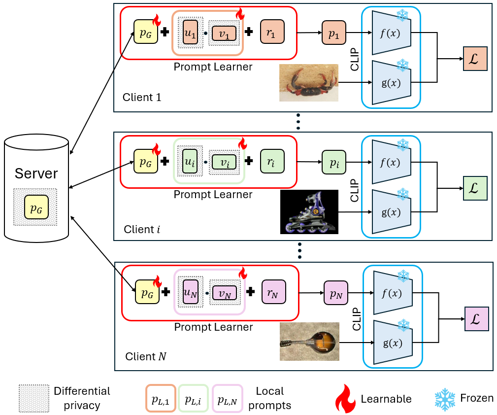
Figure 1: Architecture of DP-FPL with frozen CLIP models. Each client $i$ trains global prompt $p_{G,i}$ and local prompt $p_{L,i}$. The local prompt is factorized at each training iteration as $p_{L,i}=u_{i}v_{i}+r_{i}$.

The training process of FPL over $T$ iterations is structured as follow. For each global training round $t$, each client $i$ initializes the global prompt $p_{G,i}^{t}\leftarrow p_{G}^{t-1}$ and the local prompt ${p_{L,i}^{t}\leftarrow p_{L,i}^{t-1}}$. Client $i$ then trains their personalized prompt $p_{i}$ using their local private data and obtains the cross-entropy loss $\mathcal{L}$. At the end of the local training round, client $i$ updates their local prompt ${p_{L,i}^{t}\leftarrow p_{L,i}^{t}-\eta_{L,i}\nabla_{L,i}\mathcal{L}}$ and sends the gradient w.r.t the global prompt $\nabla_{G,i}\mathcal{L}$ to the server for aggregation. The server computes the average gradient $\nabla_{G}\leftarrow\frac{1}{N}\sum_{i=1}^{N}\nabla_{G,i}\mathcal{L}$ and updates the new global prompt to be $p_{G}^{t}\leftarrow p_{G}^{t-1}-\eta_{G}\nabla_{G}$. The learning objective function of FPL system is:

$$\min_{p_{G}}\sum_{i=1}^{N}\frac{n_{i}}{\sum_{j=1}^{N}n_{j}}\mathcal{L}_{D_{i}},$$ (3)

where $\mathcal{L}_{D_{i}}$ is the loss computed on dataset $D_{i}$ of client $i$.

3.2 Balancing Personalization and Generalization

Prior research (Aghajanyan et al., 2020; Cui et al., 2024) has demonstrated that fine tuning pre-trained LLMs with lower dimension reparameterization promotes generalization capability across various tasks. Additionally, lower intrinsic dimension improves the model utility under the effect of DP noise (Yu et al., 2021; Xu et al., 2024). Inspired by this, we adopt Low-Rank Adaptation (LoRA) (Hu et al., 2021a) in our FPL framework to balance the personalization and generalization learning under the influence of DP noise.

LoRA has been used to fine-tune pre-trained models more efficiently by introducing rank decomposition into the weight matrices of neural networks. However, LoRA has difficulty matching the performance of full-rank training in many difficult tasks (Liu et al., 2024; Biderman et al., 2024; Ivison et al., 2023; Zhuo et al., 2024). This is because low-rank decomposition methods restrict the parameter space, throwing away some of the information of the full-rank space (Konečnỳ, 2016). Recent work Cui et al. (2024) also used the low-rank approximation in non-private FPL systems, however, they factorize the local prompt only once at the beginning and train iteratively with the low-rank components. This approach can reduce the overall expressive power over the training phase. As we will show in Section 4, the loss of expressiveness can amplify the adverse effects of the DP noise, further diminishing the model’s performance. To overcome this issue, we perform the factorization process in every training round rather than only at the beginning like Cui et al. (2024), and we incorporate a residual term to compensate for the lost expressiveness. We analyze in detail the benefit of the residual term in Section 3.3. The overall personalized prompt of client $i$ can then be expressed as $p_{i}=p_{G,i}+u_{i}v_{i}+r_{i}$, where $u_{i}$ and $v_{i}$ are the factorized low-rank components and $r_{i}$ is the additional residual term.

We utilize a version of the Reparametrized Gradient Perturbation (RGP) method introduced in Yu et al. (2021) as our LoRA decomposition scheme. We perform the factorization process for each client local prompt $p_{L,i}$ in every training iteration to get the temporary low-rank prompt components $u_{i}$ and $v_{i}$. We also compute a residual term $r_{i}$ which is the remainder of the factorization process, i.e. $r_{i}=p_{L,i}-u_{i}v_{i}$. As shown by Yu et al. (2021), each client can reconstruct the gradient of $p_{L,i}$ using the gradient of the low-rank terms in back propagation as follows:

$$\nabla_{L,i}\mathcal{L}=(\nabla_{u}\mathcal{L})v_{i}+u_{i}(\nabla_{v}\mathcal{L})-u_{i}u_{i}^{T}(\nabla_{u}\mathcal{L})v_{i}$$ (4)

We note that the residual $r_{i}$ is used as part of the forward process, but it is not involved in the full-rank local prompt recomputation.

3.3 Preserving Privacy

In the personalized FPL framework, each client as a prompt provider may distribute the trained customized prompt to public users for downstream inference tasks. These fully trained prompts, if not properly protected with privacy mechanism, are vulnerable to MIA which aims to infer if an image sample was used for training or not (Wu et al., 2024). Moreover, the shared global prompt may leak information about the private data during the training process as it contains the gradient information of the loss function.

We assume that clients and server are honest. We consider adversary to be potential user with access to a trained customized prompt obtained from a FPL client. The adversary also has access to the publicly available pre-trained CLIP model for downstream inference purposes. The goal of the adversary is to infer whether an image data was part of the target FPL client’s training data utilizing the MIA. In this setting, the target client’s trained prompt $p_{i}$ is shared with a potential adversarial user and is susceptible to privacy breach, so it is necessary to protect $p_{i}$ with the DP mechanism.

One may straightforwardly apply privacy noise to the client’s trained $p_{i}$ before distributing it to public users. However, this requires a large DP noise to effectively prevent MIA (Wu et al., 2024). On the other hand, injecting noise gradually over the training phase allows for more control over the influence of noise on the model, leading to better utility (Abadi et al., 2016). In our setting, we perform gradient updates on the global prompt $p_{G,i}$ and local prompt $p_{L,i}$ of each client, so we add DP noise to the gradients w.r.t these two terms in each training step.

As part of the FPL procedure, the global prompt of each client $p_{G,i}$ is aggregated and averaged by the server, while the client’s local prompt $p_{L,i}$ stays locally. The final trained prompt $p_{i}$ is composed of the synchronized global prompt $p_{G}$ and the local prompt $p_{L,i}$. To provide privacy guarantee, we use Global Differential Privacy (GDP) for the global prompt and Local Differential Privacy (LDP) for the local prompt. This is an unconventional way of introducing DP noise to selective parts of the prompt, unlike a vanilla method that directly adds noise to the whole prompt before publishing it. We define these two DP notions as follow.

Definition 3.1.

Global Differential Privacy (GDP) A randomized mechanism $\mathcal{M}:\mathcal{D}\rightarrow\mathcal{R}$ with domain $\mathcal{D}$ and range $\mathcal{R}$ satisfies $(\epsilon,\delta)$-GDP if for any two adjacent datasets $D,D^{\prime}\in\mathcal{D}$ (i.e., datasets that differ in exactly one sample) and for any subset of outputs $\mathcal{S}\in\mathcal{R}$ it holds that

$$\text{Pr}[\mathcal{M}(D)\in\mathcal{S}]\leq e^{\epsilon}\text{Pr}[\mathcal{M}(D^{\prime})\in\mathcal{S}]+\delta$$

Definition 3.2.

Local Differential Privacy (LDP) A randomized mechanism $\mathcal{M}:\mathcal{D}\rightarrow\mathcal{R}$ with domain $\mathcal{D}$ and range $\mathcal{R}$ satisfies $(\epsilon,\delta)$-LDP if for any two adjacent samples $x,x^{\prime}\in D$ where $D\in\mathcal{D}$ and for any subset of outputs $\mathcal{S}\in\mathcal{R}$ it holds that

$$\text{Pr}[\mathcal{M}(x)\in\mathcal{S}]\leq e^{\epsilon}\text{Pr}[\mathcal{M}(x^{\prime})\in\mathcal{S}]+\delta$$

We apply GDP to the global prompt $p_{G,i}$ at the server because the impact of the GDP noise on the model utility is much smaller compared to LDP (Arachchige et al., 2019). To provide privacy guarantee for the local prompt $p_{L,i}$ which is not shared with the server for aggregation, each client needs to obfuscate $p_{L,i}$ locally with LDP noise. However, directly applying LDP noise to the full-rank local prompt $p_{L,i}$ can heavily impair the model performance (Yu et al., 2021; Xu et al., 2024). In addition, the local prompt information is predominantly captured within the low-rank components as a result of the factorization process. Therefore, we inject LDP noise only to the low-rank component $u_{i}$ and $v_{i}$ to mitigate the negative effect of privacy noise, while still effectively protecting the local prompt during the recomputation process. We note that we do not add noise to the residual component $r_{i}$ because it is not used for the local prompt recomputation.

We achieve GDP and LDP using the Gaussian noise mechanism. Given a function $f:\mathcal{D}\rightarrow\mathcal{R}$, the Gaussian noise mechanism $\mathcal{M}$ is defined as

$$\mathcal{M}(d)\triangleq f(d)+\mathcal{N}(0,\sigma^{2})$$ (5)

where $\mathcal{N}(0,\sigma^{2})$ is the normal distribution with mean $0$ and variance $\sigma^{2}$. The standard deviation $\sigma$ is typically chosen based on the function $f$’s sensitivity $S_{f}$ to satisfy an $(\epsilon,\delta)$-DP guarantee.

The two main building blocks in our approach, i.e., low-rank decomposition and DP, naturally introduce error to the training process. We conjecture that this error acts as a regularization term that prevents clients from overfitting to local data, reducing personalization and improving generalization. However, under strictly private conditions (lower rank and higher DP noise), the accumulated error may become too large and potentially destroy the personalization capability. In this case, the added residual term compensates for the regularization-like error and helps improve local learning, balancing personalization and generalization. We demonstrate the benefit of the residual term in the ablation study in Section 4.3, supporting our hypothesis. Further theoretical analysis of the residual term can be a potential future work direction.

3.4 Algorithm

We are now ready to describe our proposed method in detail, as shown in Algorithm 1.

Algorithm 1 DP-FPL

1: Initialize: $p_{G}^{0}$, $p_{L,i}^{0}$ for $i=1\dots N$, variances $\sigma_{L}$ and $\sigma_{G}$

2: for $t\leftarrow 1\ldots T$ do

3:  for $i\leftarrow 1\ldots N$ in parallel do

4:   Initialize $p_{G,i}^{t}\leftarrow p_{G}^{t-1}$ and $p_{L,i}^{t}\leftarrow p_{L,i}^{t-1}$

5:   Sample $\mathcal{B}^{t}$ from $D_{i}$

6:   Compute low-rank components $u_{i},v_{i},r_{i}\leftarrow\textbf{Factorize}(p_{L,i},k)$

7:   Recompute $p_{L,i}\leftarrow u_{i}v_{i}+r_{i}$ for forward process

8:   Obtain global text feature $f(p_{G,i}^{t})$, local text feature $f(p_{L,i}^{t})$, image feature $g(x)$ ($x\in\mathcal{B}^{t}$)

9:   Calculate loss $\mathcal{L}$ according to Equation 2 and compute gradients $\nabla_{u}\mathcal{L}$ and $\nabla_{v}\mathcal{L}$

10:   Clip gradients $\nabla_{G,i}\mathcal{L}$, $\nabla_{u}\mathcal{L}$ and $\nabla_{v}\mathcal{L}$ with threshold $C_{th}$

11:   Add local DP noise: $\tilde{\nabla_{u}}\mathcal{L}\leftarrow\nabla_{u}\mathcal{L}+\mathcal{N}(0,\sigma_{L}^{2})$ and $\tilde{\nabla_{v}}\mathcal{L}\leftarrow\nabla_{v}\mathcal{L}+\mathcal{N}(0,\sigma_{L}^{2})$

12:   Recompute noisy gradient w.r.t $\tilde{\nabla_{L,i}}\mathcal{L}$ using $\tilde{\nabla_{u}}\mathcal{L}$ and $\tilde{\nabla_{v}}\mathcal{L}$ according to equation 4

13:   Update local prompt $p_{L,i}^{t}\leftarrow p_{L,i}^{t}-\eta_{L,i}\tilde{\nabla_{L,i}}\mathcal{L}$

14:   Send $\nabla_{G,i}\mathcal{L}$ to the server

15:  end for

16:  Server computes average gradient $\nabla_{G}\leftarrow\frac{1}{N}\sum_{i=1}^{N}\nabla_{G,i}\mathcal{L}$

17:  Server adds global DP noise to $\tilde{\nabla_{G}}\leftarrow\nabla_{G}+\mathcal{N}(0,\sigma_{G}^{2})$

18:  Server updates global prompt $p_{G}^{t}\leftarrow p_{G}^{t-1}-\eta_{G}\tilde{\nabla_{G}}$

19: end for

At the initial stage, the server randomizes a starting global prompt $p_{G}^{0}$ and each client $i$ sets up their starting local prompt $p_{L,i}^{0}$ (line $1$). The variances $\sigma_{G}$ and $\sigma_{L}$ are chosen to satisfy a certain $(\epsilon,\delta)$-LDP and $(\epsilon,\delta)$-GDP guarantee. The algorithm runs for $T$ iterations. In each iteration $t$, each client updates $p_{G,i}^{t}$ to be the previously aggregated $p_{G}^{t-1}$ and $p_{L,i}^{t}$ to be the previous $p_{L,i}^{t-1}$ (line $4$). A minibatch $\mathcal{B}^{t}$ is sampled from the local dataset $D_{i}$ for training (line $5$).

Each client performs parameter factorization using the power method with rank $k$, and then recomputes the local prompt $p_{L,i}\leftarrow u_{i}v_{i}+r_{i}$ (lines $6-7$). Lines $8-9$ describe the forward pass where each client runs their local frozen CLIP model to get the text features and image feature, and uses them to calculate the loss $\mathcal{L}$ using Equation 2. Each client then computes and clips the gradient w.r.t the two low-rank prompt components $\nabla_{u}\mathcal{L}$ and $\nabla_{v}\mathcal{L}$ with threshold $C_{th}$ and add local DP noise with standard deviation $\sigma_{L}$ according to 5 (lines $10-11$).

The noisy gradient w.r.t the local prompt $\tilde{\nabla_{L,i}}\mathcal{L}$ can be reconstructed from the noisy gradients $\tilde{\nabla_{u}}\mathcal{L}$ and $\tilde{\nabla_{v}}\mathcal{L}$ using equation 4, and then is updated accordingly (lines $12-13$). Each client also computes the gradient w.r.t the global prompt $\nabla_{G,i}\mathcal{L}$ and sends it to the server for aggregation (line $14$). Upon receiving the locally computed gradients, the server computes the average gradient and adds global DP noise with standard deviation $\sigma_{G}$ to perturb the gradient (lines $16-17$). The server then updates the new global prompt for the next training round (line $18$).

Low-rank decomposition via traditional SVD method requires significant runtime. Instead, we use the power method with one iteration, significantly reducing the computational cost. Given the full-rank matrix of size $m\times n$ (assuming $m\leq n$), the computational cost of SVD scales with $\mathcal{O}(m^{2}n)$, while the power iteration only scales with $\mathcal{O}(kmn)$ where $k$ is the reduced rank and $k\ll m$.

3.5 Privacy Analysis

DP has several properties and compositions that make it easier to analyze the privacy budget in repetitive algorithms such as machine learning, where the privacy loss accumulates across multiple training iterations. When DP mechanisms are applied repeatedly to the same dataset, the overall privacy budget accumulates sequentially using the advanced composition theorem (Dwork et al., 2014). Conversely, when DP mechanisms are applied independently to disjoint subsets of a dataset, the overall privacy loss does not accumulate. In this case, the privacy guarantee remains bounded by the maximum privacy loss of any subset using parallel composition (Dwork et al., 2014). The privacy budget in term of LDP and GDP of Algorithm 1 is given by the following theorem.

Theorem 3.3.

There exist constants $c_{1},c_{2}$ so that given the number of global rounds $T$, for any $\delta>0$, DP-FPL satisfies $(\epsilon,\delta)$-LDP and $(\epsilon,\delta)$-GDP if we choose $\sigma_{L}$ and $\sigma_{G}$ as following:

$$\sigma_{L}\geq c_{1}\frac{S_{L}\sqrt{T\log(1/\delta)}}{\epsilon}\hskip 56.9055pt\sigma_{G}\geq c_{2}\frac{S_{G}\sqrt{T\log(1/\delta)}}{\epsilon}$$

where $S_{L}=\frac{C_{th}}{|\mathcal{B}|}$ and $S_{G}=\frac{C_{th}}{N|\mathcal{B}|}$ are the local and global sensitivity respectively.

Proof By definition, a single application of the Gaussian noise mechanism satisfies $(\epsilon,\delta)$-DP if we choose $\sigma\geq\frac{S\sqrt{2\log(1.25/\delta)}}{\epsilon}$ where $S$ is the sensitivity. Under the advanced composition theorem of DP, the Gaussian noise mechanism after $T$ training steps results in an accumulated privacy loss of $(\mathcal{O}(\epsilon\sqrt{T}),\delta)$-DP. Thus, to achieve $(\epsilon,\delta)$-DP, one would need to choose

$$\sigma\geq c\frac{S\sqrt{T\log(1/\delta)}}{\epsilon}$$ (6)

for the Gaussian noise mechanism where $c^{\prime}$ is a constant.

Applying Equation 6, we can choose $\sigma_{L}\geq c_{1}\frac{S_{L}\sqrt{T_{L}\log(1/\delta)}}{\epsilon}$ where $c_{1}$ is a constant to make Algorithm 1 satisfy $(\epsilon,\delta)$-LDP with respect to each client. Since each client $i$ operates the Gaussian noise mechanism independently on disjoint local subset $D_{i}$ of the global dataset $D$, the release of all clients’ noisy mechanism output still satisfies $(\epsilon,\delta)$-LDP by the parallel composition of DP. Similarly, by choosing $\sigma_{G}\geq c_{2}\frac{S_{G}\sqrt{T\log(1/\delta)}}{\epsilon}$ according to Equation 6, DP-FPL satisfies $(\epsilon,\delta)$-GDP.

We proved in the theorem above that Algorithm 1 satisfies $(\epsilon,\delta)$-LDP and $(\epsilon,\delta)$-GDP when publishing the customized prompt to potential users. Since the GDP noise is added to the aggregated gradient, the distribution of the aggregated gradient to all clients also satisfies $(\epsilon,\delta)$-GDP by the post-processing property of DP. According to Theorem 3.3, we can calculate the standard deviations $\sigma_{L}$ and $\sigma_{G}$ to achieve a certain $(\epsilon,\delta)$-LDP and $(\epsilon,\delta)$-GDP. The pair $\epsilon,\delta$ can be chosen to match a desired MIA accuracy rate, preferably lower than random guess ($50\%$) (Thudi et al., 2022).

4 Experiments

4.1 Setup

Datasets. We select four visual classification datasets to investigate the task of balancing personalization, generalization and privacy: Caltech101 (Fei-Fei et al., 2004), OxfordPets (Parkhi et al., 2012), OxfordFlowers (Nilsback & Zisserman, 2008) and Food101 (Bossard et al., 2014). We utilize the pathological data split among $10$ clients. Each client model is trained on its local classes, and evaluated on both its local classes for personalization capability and neighbor classes (classes owned by other clients) for generalization capability. We also evaluate the large-scale dataset CIFAR-100 (Krizhevsky et al., 2009) with the Dirichlet data split among $25$ and $50$ clients. The final test accuracy is obtained by averaging the performance across all clients. Details of our implementation and hyperparameters are provided in the appendix. Our code is available at https://anonymous.4open.science/r/DP-FPL-84F8.

Table 2: Mean test accuracy on local classes averaged across $10$ clients. The baseline FedPGP and our method DP-FPL have factorization on the local prompt with rank $8$.

Dataset	Noise $\epsilon$	PromptFL	FedOTP	FedPGP	DP-FPL
	None	94.45$\pm$0.30	97.06$\pm$0.48	95.21$\pm$0.19	96.06$\pm$0.18
Caltech	$0.4$	82.53$\pm$0.52	95.09$\pm$0.50	95.12$\pm$0.46	95.74$\pm$0.63
101	$0.2$	81.52$\pm$0.45	87.61$\pm$0.58	90.98$\pm$0.40	95.28$\pm$0.46
	$0.1$	80.42$\pm$0.65	84.98$\pm$0.39	80.01$\pm$0.39	92.71$\pm$0.38
	$0.05$	78.61$\pm$1.39	83.61$\pm$0.38	77.24$\pm$0.38	87.64$\pm$0.79
	$0.01$	78.52$\pm$1.68	78.86$\pm$0.38	77.23$\pm$0.37	85.21$\pm$0.85
	None	76.85$\pm$0.96	99.63$\pm$0.2	94.66$\pm$0.31	96.91$\pm$0.76
Oxford	$0.4$	74.36$\pm$0.26	80.03$\pm$0.93	86.56$\pm$0.69	95.13$\pm$0.52
Pets	$0.2$	73.56$\pm$0.16	65.97$\pm$0.89	67.11$\pm$0.44	93.09$\pm$0.43
	$0.1$	72.77$\pm$0.16	59.54$\pm$0.58	63.21$\pm$0.62	85.25$\pm$0.18
	$0.05$	52.39$\pm$0.53	58.97$\pm$1.02	57.98$\pm$0.97	81.26$\pm$1.10
	$0.01$	43.68$\pm$0.67	54.08$\pm$1.04	45.49$\pm$1.33	73.71$\pm$0.40
	None	84.04$\pm$0.32	97.84$\pm$1.16	79.11$\pm$0.45	85.75$\pm$0.62
Oxford	$0.4$	60.31$\pm$1.28	79.89$\pm$0.80	77.13$\pm$0.52	80.09$\pm$1.41
Flowers	$0.2$	40.33$\pm$0.83	65.96$\pm$0.96	70.77$\pm$0.61	76.75$\pm$1.05
	$0.1$	38.25$\pm$1.37	42.31$\pm$0.71	52.42$\pm$1.58	72.11$\pm$1.37
	$0.05$	37.18$\pm$0.92	38.89$\pm$0.66	39.52$\pm$0.77	69.80$\pm$1.34
	$0.01$	36.11$\pm$0.60	33.98$\pm$0.63	35.23$\pm$0.64	51.55$\pm$1.07
	None	86.50$\pm$0.26	86.65$\pm$0.23	84.40$\pm$0.09	86.08$\pm$0.12
Food	$0.4$	78.70$\pm$0.39	79.45$\pm$0.23	80.58$\pm$1.52	81.45$\pm$0.21
101	$0.2$	71.84$\pm$0.91	77.36$\pm$0.41	77.72$\pm$1.50	81.25$\pm$0.18
	$0.1$	69.00$\pm$0.40	70.48$\pm$1.39	75.18$\pm$0.22	80.57$\pm$0.46
	$0.05$	68.36$\pm$1.23	62.98$\pm$1.25	73.72$\pm$1.04	78.23$\pm$0.43
	$0.01$	67.47$\pm$1.20	54.70$\pm$1.12	71.82$\pm$1.19	77.45$\pm$0.40

Baselines. To demonstrate the effectiveness of our proposed method in balancing personalization, generalization and privacy, we compare with three baseline cases: (1) PromptFL (Guo et al., 2023b), (2) FedOTP (Li et al., 2024) and (3) FedPGP (Cui et al., 2024). More details of the baselines are listed in the appendix.

Privacy levels. We consider different noise levels for LDP and GDP: ${\epsilon=\{0.01,0.05},0.1,0.2,0.4\}$. We pick $\delta=10^{-5}$ and the clipping threshold $C_{th}=10$. We provide details of how the noise is added to each baseline in the appendix.

4.2 Performance Results

Improving personalization in private setting. Table 2 shows the average test accuracy over the last $10$ epochs on local classes. In the non-private scenario (i.e., Noise = None), FedOTP shows the highest utility, however, as we add more noise, DP-FPL comes in the first place with the highest local classes accuracy. Under strict privacy levels ($\epsilon=0.01$), we see a noticeable decrease in test accuracy. Nevertheless, DP-FPL still consistently outperforms other baselines across all datasets, showing the robustness of our method even under strictly private conditions. Table 4 shows the overall accuracy utilizing a Dirichlet data split and ResNet50 as the backbone model. As shown in Table 4, DP-FPL demonstrates superior performance compared to baseline methods across all datasets. This shows the effectiveness and applicability of our approach in various complex settings, including different data distributions, models, and number of clients.

Privacy improves generalization. Table 3 shows the average test accuracy over the last $10$ epochs on neighbor classes. Similar to local classes, DP-FPL exhibits the highest utility in neighbor classes under the presence of DP noise. As expected, the accuracy degrade for higher noise levels, however, we see an improvement in Caltech101 utility when we increase privacy level from $0.4$ to $0.1$. This is because privacy noise act as a form of regularization that prevents overfitting, and hence improving generalization. Nevertheless, when the noise level is large enough ($\epsilon=\{0.01,0.05\}$), the overall utility is degraded and the neighbor accuracy no longer improves.

Table 3: Mean test accuracy on neighbor classes averaged across $10$ clients. The baseline FedPGP and our method DP-FPL have factorization on the local prompt with rank $8$.

Dataset	Noise $\epsilon$	PromptFL	FedOTP	FedPGP	DP-FPL
	None	92.88$\pm$0.19	74.91$\pm$0.30	93.44$\pm$0.75	91.54$\pm$0.15
Caltech	$0.4$	82.66$\pm$1.22	84.26$\pm$0.84	88.24$\pm$0.78	88.58$\pm$0.38
101	$0.2$	81.93$\pm$1.47	84.08$\pm$0.98	86.05$\pm$0.79	89.72$\pm$0.98
	$0.1$	80.83$\pm$0.72	78.91$\pm$1.02	79.31$\pm$0.82	90.02$\pm$1.47
	$0.05$	79.96$\pm$0.40	73.37$\pm$1.03	75.62$\pm$0.82	82.76$\pm$1.12
	$0.01$	78.89$\pm$0.33	73.54$\pm$1.00	75.60$\pm$0.82	80.60$\pm$0.57
	None	76.34$\pm$0.37	65.63$\pm$0.14	89.71$\pm$0.49	80.19$\pm$0.85
Oxford	$0.4$	74.43$\pm$0.87	60.95$\pm$0.81	72.54$\pm$0.54	81.82$\pm$0.42
Pets	$0.2$	73.74$\pm$0.82	59.74$\pm$0.84	61.68$\pm$0.46	80.67$\pm$0.28
	$0.1$	73.12$\pm$0.39	58.83$\pm$0.93	59.79$\pm$0.79	77.12$\pm$0.52
	$0.05$	52.44$\pm$0.89	54.08$\pm$0.89	51.63$\pm$1.01	74.13$\pm$0.48
	$0.01$	38.27$\pm$0.86	53.63$\pm$0.91	40.20$\pm$0.42	71.89$\pm$0.48
	None	69.44$\pm$0.61	38.29$\pm$1.09	75.79$\pm$0.87	69.51$\pm$0.45
Oxford	$0.4$	48.03$\pm$0.69	56.65$\pm$0.77	65.93$\pm$0.86	67.67$\pm$0.45
Flowers	$0.2$	38.19$\pm$0.97	55.44$\pm$0.90	63.49$\pm$0.65	67.51$\pm$0.58
	$0.1$	37.76$\pm$1.23	37.53$\pm$1.09	46.24$\pm$1.86	66.44$\pm$1.51
	$0.05$	38.78$\pm$1.18	33.48$\pm$1.00	35.27$\pm$1.28	56.75$\pm$1.85
	$0.01$	34.81$\pm$1.19	31.26$\pm$0.96	34.72$\pm$1.60	43.21$\pm$1.72
	None	86.19$\pm$0.13	84.03$\pm$0.33	86.23$\pm$0.06	86.08$\pm$0.11
Food	$0.4$	76.88$\pm$0.23	80.11$\pm$0.47	78.94$\pm$1.07	81.00$\pm$0.25
101	$0.2$	70.99$\pm$0.83	76.44$\pm$0.62	77.21$\pm$0.90	80.79$\pm$0.22
	$0.1$	67.80$\pm$1.59	73.12$\pm$1.65	76.92$\pm$0.83	78.14$\pm$0.53
	$0.05$	66.76$\pm$1.27	71.82$\pm$0.79	73.61$\pm$1.35	77.18$\pm$0.50
	$0.01$	61.42$\pm$1.49	67.08$\pm$1.11	72.99$\pm$1.53	76.87$\pm$0.62

Table 4: Mean test accuracy averaged across all clients under Dirichlet data distribution. The baseline FedPGP and our method DP-FPL have factorization on the local prompt with rank $8$.

Noise	CIFAR-100 with $25$ clients				CIFAR-100 with $50$ clients
$\epsilon$	PromptFL	FedOTP	FedPGP	DP-FPL	PromptFL	FedOTP	FedPGP	DP-FPL
None	71.20$\pm$0.18	68.13$\pm$0.33	71.54$\pm$0.17	69.84$\pm$0.19	71.30$\pm$0.10	68.57$\pm$0.14	70.82$\pm$0.12	69.48$\pm$0.11
$0.4$	53.69$\pm$0.53	47.22$\pm$0.97	58.87$\pm$0.35	66.23$\pm$0.23	55.44$\pm$0.31	58.23$\pm$0.42	58.43$\pm$0.51	66.40$\pm$0.18
$0.2$	53.02$\pm$0.39	47.02$\pm$1.13	56.75$\pm$0.31	62.92$\pm$0.30	54.65$\pm$0.29	57.09$\pm$0.40	56.34$\pm$0.44	64.39$\pm$0.29
$0.1$	50.86$\pm$0.68	46.95$\pm$1.06	55.76$\pm$0.33	59.53$\pm$0.25	53.17$\pm$1.06	57.05$\pm$0.22	53.39$\pm$0.48	60.49$\pm$0.26
$0.05$	50.20$\pm$0.40	44.71$\pm$1.16	53.80$\pm$0.30	57.97$\pm$0.16	53.23$\pm$0.83	55.00$\pm$0.37	52.38$\pm$0.49	58.35$\pm$0.30
$0.01$	50.65$\pm$0.41	44.27$\pm$1.17	51.75$\pm$0.34	53.31$\pm$0.35	51.92$\pm$1.56	54.53$\pm$0.29	52.32$\pm$0.46	56.09$\pm$0.56

4.3 Ablation Study

In this subsection, we investigate the efficacy of the key parameters that directly affect the tradeoff between personalization, generalization, and privacy: residual term, noise level $\epsilon$ and rank value. The results for Caltech101 are presented in Figure 2; we include other dataset results in the appendix.

Effect of residual term. We investigate the effectiveness of the residual term by separately testing the model without the residual component in Figure 2. We note that this setting is different from FedPGP because the factorization process is performed every training round instead of at the beginning. In Figure 2, we observe better performance in both local and neighbor classes when incorporating the residual term. The difference in accuracy is more prominent under strict privacy conditions (rank $1$ and $\epsilon=0.01$), confirming our conjecture about the benefit of the residual described in Section 3.3. Lower rank and higher noise significantly reduce the overall utility due to the large accumulated error, and the residual term plays a crucial role in improving local learning, balancing personalization and generalization.

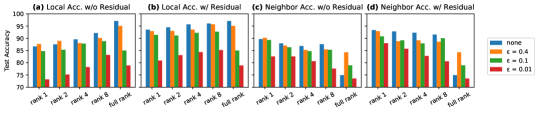
Figure 2: Test accuracy of ablation study on noise level, rank and residual term for Caltech101

Effect of privacy noise $\epsilon$. We study how different privacy level affects the model performance on both local and neighbor classes in Figure 2 (b) and (c). As expected, the local classes accuracy gradually decreases when noise level increases. However, we see some unexpected improvement in neighbor utility when we increase DP noise from $0.4$ to $0.1$. As explained in Section 4.2, certain privacy noise range acts like regularization error that prevents overfitting, resulting in better generalization for higher noise level.

Effect of factorization rank. We explore the impact of the factorization rank by comparing different rank values with full-rank setting in Figure 2 (b) and (c). Intuitively, higher rank values lead to better performance, however, this is not always the case. For local classes, rank $8$ generally performs better than full-rank under higher noise levels ($\epsilon=\{0.01,0.1\}$). Lower-rank has fewer entries, hence the amount of noise added is less than full-rank for the same level of privacy guarantee, which leads to better accuracy. For neighbor classes, lower rank value tends to have higher utility because lower rank introduces more regularization error that prevents overfitting and improves generalization.

5 Conclusion

In this paper, we presented a novel approach to address the critical challenges of personalization, generalization, and privacy in FPL for multimodal LLMs. Our proposed framework leverages low-rank decomposition to balance the tradeoffs between these competing objectives. By decomposing the local prompts into low-rank components iteratively while incorporating a residual term, our method effectively preserves both generalization and personalization. Moreover, we introduced a privacy-preserving mechanism that applies both global and local DP to safeguard sensitive client data. Unlike conventional methods, we selectively applied DP noise to the low-rank components, allowing us to maintain privacy without significantly degrading model performance. The critical role of the residual term in mitigating the effects of DP noise was also demonstrated, highlighting its importance for maintaining model expressiveness and personalization.

Appendix A Experimental Details

A.1 Datasets

Caltech101 (Fei-Fei et al., 2004) is an image dataset that contains images from $101$ object categories (e.g., “helicopter”, “elephant” and “chair” etc.). There are about $40$ to $800$ images for each object category, but most categories have about $50$ images. The dataset is available for download on http://www.vision.caltech.edu/Image_Datasets/Caltech101/101_ObjectCategories.tar.gz. The dataset contains $6,593$ samples, including $4,128$ training samples and $2,465$ testing samples.

Oxford Pets (Parkhi et al., 2012) is an image dataset with $37$ object classes that can be downloaded at https://www.robots.ox.ac.uk/~vgg/data/pets/data/images.tar.gz. The dataset consists of $6,613$ pet images with roughly $200$ images for each class. The dataset is divided into training set of $2,944$ images and test set of $3,669$ images.

Oxford Flowers (Nilsback & Zisserman, 2008) is an image classification dataset consisting of $102$ flower categories, each class has between $40$ and $258$ images. The dataset is can be retrieved at https://www.robots.ox.ac.uk/~vgg/data/flowers/102/102flowers.tgz. There are $6,556$ total images, including $4,093$ training images and $2,463$ testing images.

Food101 (Bossard et al., 2014) is a large-scale dataset containing images of $101$ different types of food. The dataset is are available for download at https://data.vision.ee.ethz.ch/cvl/datasets_extra/food-101/. There are $80,800$ total images, and we split the dataset into train set of size $50,500$ and test set of size $30,300$.

CIFAR-100 (Krizhevsky et al., 2009) is a another large-scale dataset containing images of $100$ different object classes. The dataset is are available for download via torchvision.datasets.CIFAR10. The dataset consists of $60,000$ $32$x$32$ images, with $6,000$ images per class. We divide the dataset into training set of $50,000$ images and test set of $10,000$ images.

A.2 Implementation Details

For the first four datasets Caltech101, OxfordPets, OxfordFlowers and Food101, we use the Vision Transformer ViT-B16 (Dosovitskiy, 2020) as the backbone for the frozen CLIP model for Caltech101, OxfordPets, OxfordFlowers and Food101. For each dataset, we run experiments with $N=10$ clients for $T=100$ global training rounds. We use batch size $|\mathcal{B}|=32$ for training and $|\mathcal{B}|=100$ for testing. We set the global learning rate $\eta_{G}=0.0001$ and local learning rate $\eta_{L}=0.0001$ with SGD optimizer.

We adopt the Pathological setting for data heterogeneity among clients as implemented in https://github.com/KaiyangZhou/CoOp/blob/main/DATASETS.md. The class labels are splitted randomly among $10$ clients without overlapping, and each client owns disjoint set of local classes. For each client, we train the local model on data associated with their assigned local classes. We then evaluate each client’s local model on two test sets: local class test set for personalization and neighbor class test set for generalization. The local class test set involve all the test image associated with the client’s local class labels. The neighbor class test set is the set of all test images whose labels are owned by other clients.

For CIFAR-100, we adopt ResNet50 (He et al., 2016) as the backbone model and run experiments with $N=25$ and $N=50$ clients for $T=200$ global training rounds. We use batch size $|\mathcal{B}|=32$ for training and $|\mathcal{B}|=100$ for testing. We set the global learning rate $\eta_{G}=0.0001$ and local learning rate $\eta_{L}=0.0001$ with SGD optimizer. We use Dirichlet data distribution to simulate the real-world non-IID setting with parameter $\alpha=0.3$. The test accuracy is averaged across all clients.

We provide a summary of the experiment set up in Table 5 below.

Table 5: Details of datasets and experimental set up

Dataset	Data distribution	Model	Number	Number of	Training	Testing
			of clients	training rounds	batch size	batch size
Caltech101	Pathological	ViT-B16	10	100	32	100
OxfordPets	Pathological	ViT-B16	10	100	32	100
OxfordFlowers	Pathological	ViT-B16	10	100	32	100
Food101	Pathological	ViT-B16	10	100	32	100
CIFAR-100	Dirichlet	ResNet50	25, 50	200	32	100

For the prompt learner, the length of prompt vectors is $b=16$ with a dimension of $d=512$, and the token position is “end” with “random” initialization. For the factorization process, we experiment with four different decomposition rank $1,2,4,8$. We consider three different DP noises with privacy level from low to high: $\epsilon\in\{0.4,0.2,0.1\}$. The clipping threshold is chosen to be $C_{th}=10$ for both GDP and LDP applications.

For the baseline methods, we consider three settings: PromptFL (Guo et al., 2023b), FedOTP (Li et al., 2024) and FedPGP (Cui et al., 2024) with the main difference lies in the prompt learner structure. We describe each baseline in detail below.

1. PromptFL: PromptFL follows the traditional federated learning framework where each client has one single prompt $p_{i}$ and the aggregated prompt is the average of all clients’ $p_{i}$. In this setting, the privacy noise is added directly to each client’s $p_{i}$ before sharing with the server for aggregation.

2. FedOTP: In FedOTP, each client’s customized prompt $p_{i}$ involves two full-rank global prompt $p_{G,i}$ and local prompt $p_{L,i}$. To incorporate privacy, the GDP noise is added to the averaged $p_{G}$ by the server and the LDP noise is added to each client’s local prompt $p_{L,i}$.

3. FedPGP: In FedPGP, each client’s customized prompt $p_{i}$ includes a full-rank global prompt $p_{G,i}$ and two low-rank local components $u_{i},v_{i}$. Each client then train three parameters $p_{G,i}$, $u_{i}$ and $v_{i}$ across the training process. In this baseline, the GDP noise is added to the averaged $p_{G}$ by the server and the LDP noise is added to the two low-rank terms $u_{i},v_{i}$ of each client.

We run our experiment on a computer cluster, each node has a 6x NVIDIA Tesla V100 GPUs with 32 GiB of memory and 512 GiB RAM and 2x IBM Power 9 processors. The final result is the mean accuracy over the last $10$ training epochs, averaged across all clients.

A.3 Membership Inference Attack

In this section, we evaluate the privacy-preserving performance of our method DP-FPL against Membership Inference Attack (MIA). We implement MIA as described in Shokri et al. (2017), where the goal of the attack is to infer the appearance of data samples in one client’s training dataset. We first train a set of $50$ shadow models with the same model architecture as the target client’s model. The shadow models generate synthetic training data that is used to train the attack model. The attack model is a two-layer MLP and a classification head that predicts if a given sample is part of the target client’s training data or not. We run the attack on Caltech101, Oxford Pets and Oxford Flowers with different privacy levels. For each dataset, we perform separate attack on each class and compute the average success rate, i.e. percentage of correct guesses.

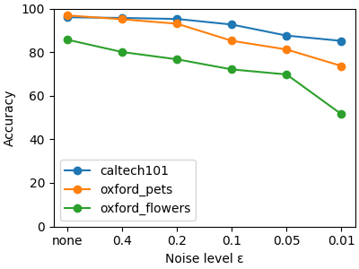
(a) Target local accuracy

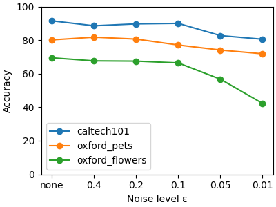
(b) Target neighbor accuracy

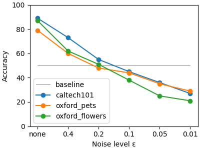
(c) MIA accuracy

Figure 3: Target model performance (a, b) and MIA performance (c) with rank $8$. The baseline of MIA accuracy is set to $50\%$ (random guessing).

Figure 3 demonstrates the performance of the target model (local and neighbor classes) and the MIA. We set the MIA baseline accuracy to be $50\%$, representing the expected success rate of random guessing. Looking at Figure 3(c), the MIA accuracy is low ($<50\%$) when $\epsilon=0.2$ for Oxford Pets and $\epsilon=0.1$ for Caltech101 and Oxford Flowers. In addition, $\epsilon=0.1$ causes minimal loss in the target model accuracy for both local and neighbor classes (Figures 3(a) and 3(b)). Therefore, one can balance the utility-privacy tradeoff by setting $\epsilon=0.1$ for any dataset. This shows that our approach effectively protects the training data from MIA while still maintaining good model performance.

A.4 Additional Experimental Results

In this section, we include additional results from the experiments introduced in Section 4 to further investigate how the DP parameter $\epsilon$, factorization rank and the residual term affect the tradeoff between personalization, generalization and privacy guarantee. Figures 4, 5 and 6 continue the ablation study on the effect of the key parameters that directly affect the tradeoff: residual term, noise level and rank. We summarize the results for each dataset below.

Figure 4 shows the test accuracy with different parameter settings for Oxford Pets. In general, there is an increase in both local and neighbor classes when incorporating the residual term, highlighting the benefit of the residual in model utility in different datasets. The difference in accuracy is more consistent across different noise and rank values compared to Figure 2. In addition, there is minimal growth in accuracy when we increase the rank value. Therefore, it is beneficial to set any rank value for this particular dataset.

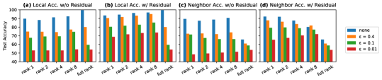
Figure 4: Test accuracy of ablation study on noise level, rank and residual term for Oxford Pets

Figure 5 shows the test accuracy with different parameter settings for Oxford Flowers. The addition of the residual term still improves the overall utility, though the benefit is modest for this dataset. Similar to Oxford Pets, the rank value does not significantly affect the accuracy for both local and neighbor classes. We also observe more drastic drop in accuracy under strong privacy level ($\epsilon=0.01$). Overall, it is more difficult to balance the tradeoff for Oxford Flowers. One needs to sacrifice strong data protection and set $\epsilon\geq 0.1$ to achieve good personalization and generalization utility.

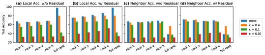
Figure 5: Test accuracy of ablation study on noise level, rank and residual term for Oxford Flowers

Figure 6 shows the test accuracy with different parameter settings for Food101. We see an overall increase in local and neighbor accuracy with the introduction of the residual term, and the difference is more significant under higher noise level. In addition, there is minimal reduction in model utility when we increase privacy noise. This behavior is consistent across all rank values, indicating the robustness of our method under strict privacy constraints.

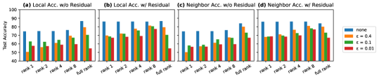
Figure 6: Test accuracy of ablation study on noise level, rank and residual term for Food101

Overall, the affect of the key parameters (noise level, rank and residual term) on the tradeoff between personalization, generalization and privacy varies widely among different datasets. Nonetheless, the results across all datasets show consistent trends, indicating the effectiveness and applicability of our method.

For completeness, we include Tables 6, 7, 8 and 9 which detail the test accuracy with standard deviation of all the ablation experiments demonstrated in Figures 2, 4, 5 and 6.

Table 6: Mean test accuracy of our method averaged across $10$ clients under non-private setting (without any DP noise).

Dataset	Rank	Local classes		Neighbor classes
		without residual	with residual	without residual	with residual
	1	86.64$\pm$0.78	93.55$\pm$0.18	89.70$\pm$0.81	93.40$\pm$0.28
Caltech101	2	87.54$\pm$0.83	94.51$\pm$0.17	87.95$\pm$0.42	92.79$\pm$0.72
	4	89.57$\pm$0.47	95.69$\pm$0.57	86.86$\pm$0.72	92.32$\pm$0.71
	8	92.12$\pm$0.47	96.06$\pm$0.39	87.58$\pm$0.17	91.54$\pm$0.73
	1	89.78$\pm$0.71	93.46$\pm$0.63	89.54$\pm$0.71	92.17$\pm$0.27
Oxford Pets	2	88.24$\pm$0.73	94.49$\pm$0.91	87.37$\pm$0.38	91.96$\pm$0.71
	4	91.28$\pm$0.64	96.36$\pm$0.28	88.70$\pm$0.83	87.61$\pm$0.53
	8	92.42$\pm$0.81	96.91$\pm$0.58	90.71$\pm$1.09	80.19$\pm$0.64
	1	67.41$\pm$0.19	75.45$\pm$0.20	67.22$\pm$0.63	71.49$\pm$0.71
Oxford Flowers	2	66.18$\pm$0.89	78.56$\pm$0.90	66.16$\pm$0.10	69.76$\pm$1.11
	4	67.04$\pm$0.61	81.53$\pm$0.49	67.02$\pm$0.39	68.33$\pm$0.32
	8	68.35$\pm$0.61	85.75$\pm$0.91	68.75$\pm$0.47	69.51$\pm$0.61
	1	74.66$\pm$1.14	86.12$\pm$0.38	74.58$\pm$0.51	85.97$\pm$0.72
Food101	2	74.91$\pm$0.38	86.06$\pm$0.27	74.96$\pm$0.49	85.89$\pm$0.52
	4	74.95$\pm$0.91	86.18$\pm$0.63	74.84$\pm$0.99	86.16$\pm$1.06
	8	76.95$\pm$1.02	86.08$\pm$0.95	76.02$\pm$0.77	86.08$\pm$0.69

Table 7: Mean test accuracy of DP-FPL averaged across $10$ clients. The DP noise is set to $\epsilon=0.4$.

Dataset	Rank	Local classes		Neighbor classes
		without residual	with residual	without residual	with residual
	1	87.66$\pm$0.79	92.93$\pm$1.18	90.19$\pm$1.11	92.94$\pm$0.68
Caltech101	2	88.98$\pm$1.02	93.03$\pm$0.90	86.99$\pm$1.34	88.82$\pm$0.79
	4	88.01$\pm$1.21	93.58$\pm$0.87	85.20$\pm$1.03	89.15$\pm$0.90
	8	90.13$\pm$1.19	95.74$\pm$0.63	85.46$\pm$1.08	88.58$\pm$0.38
	1	74.87$\pm$0.69	90.43$\pm$0.79	72.41$\pm$0.49	87.83$\pm$0.95
Oxford Pets	2	74.66$\pm$0.88	91.67$\pm$0.62	72.69$\pm$0.33	86.26$\pm$0.42
	4	74.24$\pm$0.74	93.22$\pm$0.40	71.83$\pm$0.39	83.53$\pm$0.60
	8	77.22$\pm$0.82	95.13$\pm$0.52	73.86$\pm$0.42	81.82$\pm$0.42
	1	62.48$\pm$0.83	75.45$\pm$0.55	64.41$\pm$0.58	71.49$\pm$0.55
Oxford Flowers	2	65.67$\pm$0.96	77.39$\pm$0.69	64.53$\pm$0.75	70.97$\pm$0.58
	4	66.23$\pm$0.79	78.62$\pm$1.04	63.97$\pm$0.77	68.10$\pm$0.67
	8	68.03$\pm$1.41	80.09$\pm$0.51	63.22$\pm$0.88	67.67$\pm$0.45
	1	50.55$\pm$1.05	69.76$\pm$0.43	50.29$\pm$1.14	68.11$\pm$0.94
Food101	2	56.07$\pm$0.85	72.05$\pm$0.66	57.10$\pm$1.13	71.15$\pm$0.65
	4	61.02$\pm$1.09	77.76$\pm$0.98	61.25$\pm$0.58	76.48$\pm$0.57
	8	69.53$\pm$0.20	81.45$\pm$1.01	67.52$\pm$0.40	81.00$\pm$0.90

Table 8: Mean test accuracy of DP-FPL averaged across $10$ clients. The DP noise is set to $\epsilon=0.2$.

Dataset	Rank	Local classes		Neighbor classes
		without residual	with residual	without residual	with residual
	1	87.79$\pm$0.81	92.16$\pm$0.38	90.43$\pm$0.91	91.61$\pm$1.02
Caltech101	2	88.99$\pm$0.63	93.38$\pm$0.82	87.22$\pm$0.47	90.55$\pm$0.49
	4	89.25$\pm$0.61	94.22$\pm$0.54	85.31$\pm$0.28	90.73$\pm$0.10
	8	91.75$\pm$0.19	95.28$\pm$0.93	86.56$\pm$0.71	89.72$\pm$0.83
	1	70.06$\pm$0.73	89.79$\pm$0.59	73.27$\pm$0.51	87.69$\pm$1.08
Oxford Pets	2	72.71$\pm$0.42	90.12$\pm$0.49	72.04$\pm$0.39	86.74$\pm$0.18
	4	72.27$\pm$0.84	91.45$\pm$0.65	70.16$\pm$0.77	83.62$\pm$0.94
	8	73.73$\pm$0.94	93.09$\pm$0.30	71.04$\pm$0.55	80.67$\pm$0.69
	1	55.18$\pm$0.92	72.19$\pm$0.17	64.53$\pm$0.81	70.35$\pm$0.97
Oxford Flowers	2	59.52$\pm$0.53	73.58$\pm$0.57	61.41$\pm$0.31	70.50$\pm$0.29
	4	63.89$\pm$0.83	75.18$\pm$0.57	61.50$\pm$0.81	68.65$\pm$0.46
	8	63.86$\pm$0.86	76.75$\pm$0.97	62.65$\pm$0.65	67.51$\pm$0.73
	1	57.38$\pm$0.35	69.94$\pm$0.82	58.11$\pm$0.37	63.63$\pm$0.92
Food101	2	59.22$\pm$0.16	70.52$\pm$0.75	58.17$\pm$0.57	67.64$\pm$0.38
	4	65.12$\pm$0.52	75.11$\pm$0.46	64.74$\pm$0.44	70.21$\pm$0.80
	8	70.16$\pm$0.32	81.25$\pm$0.51	70.21$\pm$0.75	80.79$\pm$0.17

Table 9: Mean test accuracy of DP-FPL averaged across $10$ clients. The DP noise is set to $\epsilon=0.1$.

Dataset	Rank	Local classes		Neighbor classes
		without residual	with residual	without residual	with residual
	1	84.73$\pm$0.32	91.39$\pm$0.58	89.33$\pm$0.85	90.81$\pm$0.59
Caltech101	2	85.32$\pm$0.38	91.11$\pm$0.86	86.32$\pm$0.28	89.18$\pm$0.67
	4	87.82$\pm$0.81	92.26$\pm$1.28	84.73$\pm$0.97	87.92$\pm$0.80
	8	88.82$\pm$0.84	92.71$\pm$0.61	85.32$\pm$0.86	90.02$\pm$0.48
	1	67.59$\pm$0.19	80.41$\pm$0.38	71.47$\pm$0.32	79.24$\pm$0.61
Oxford Pets	2	69.22$\pm$0.48	81.65$\pm$1.06	67.38$\pm$0.27	79.65$\pm$0.59
	4	69.35$\pm$0.89	82.73$\pm$0.49	66.11$\pm$0.66	78.73$\pm$0.87
	8	74.48$\pm$0.91	85.25$\pm$0.30	66.10$\pm$0.49	77.12$\pm$0.63
	1	54.18$\pm$0.65	66.78$\pm$1.02	59.51$\pm$0.75	66.93$\pm$0.49
Oxford Flowers	2	57.16$\pm$0.39	66.21$\pm$0.29	65.35$\pm$0.64	65.21$\pm$0.94
	4	59.71$\pm$0.83	67.32$\pm$0.27	67.71$\pm$0.41	67.26$\pm$0.32
	8	59.81$\pm$0.97	72.11$\pm$1.05	66.98$\pm$0.38	66.44$\pm$0.17
	1	62.75$\pm$0.37	68.65$\pm$0.81	58.05$\pm$0.42	68.60$\pm$0.28
Food101	2	62.43$\pm$0.76	71.84$\pm$0.95	58.86$\pm$0.26	69.66$\pm$0.93
	4	64.66$\pm$0.75	75.64$\pm$0.41	65.22$\pm$0.28	72.61$\pm$0.30
	8	67.20$\pm$0.48	80.57$\pm$0.83	67.06$\pm$0.99	78.14$\pm$0.37

Table 10: Mean test accuracy of DP-FPL averaged across $10$ clients. The DP noise is set to $\epsilon=0.05$.

Dataset	Rank	Local classes		Neighbor classes
		without residual	with residual	without residual	with residual
	1	78.62$\pm$0.24	81.59$\pm$1.55	78.75$\pm$0.23	79.07$\pm$1.59
Caltech101	2	78.63$\pm$0.18	85.42$\pm$0.93	77.67$\pm$0.34	77.42$\pm$0.92
	4	78.57$\pm$0.48	85.05$\pm$1.06	77.51$\pm$0.48	82.28$\pm$1.07
	8	78.72$\pm$0.49	87.64$\pm$0.98	76.83$\pm$0.42	82.76$\pm$1.69
	1	63.28$\pm$0.57	70.60$\pm$1.30	61.75$\pm$0.58	72.18$\pm$1.32
Oxford Pets	2	63.32$\pm$0.68	73.66$\pm$0.94	61.76$\pm$0.70	72.62$\pm$1.39
	4	64.26$\pm$0.91	74.29$\pm$1.35	61.71$\pm$0.91	68.73$\pm$1.31
	8	65.22$\pm$0.89	81.26$\pm$1.00	61.69$\pm$0.62	74.13$\pm$0.99
	1	32.98$\pm$1.13	59.62$\pm$0.99	29.91$\pm$0.61	46.80$\pm$0.91
Oxford Flowers	2	32.84$\pm$1.80	59.74$\pm$1.05	30.02$\pm$1.14	49.19$\pm$1.47
	4	32.45$\pm$1.15	65.72$\pm$1.17	30.40$\pm$0.75	50.32$\pm$1.18
	8	33.09$\pm$1.62	69.80$\pm$0.94	30.21$\pm$1.28	56.75$\pm$1.23
	1	58.72$\pm$0.36	67.19$\pm$0.92	56.37$\pm$0.25	67.09$\pm$0.46
Food101	2	57.01$\pm$0.41	67.71$\pm$1.42	55.59$\pm$0.77	67.27$\pm$0.57
	4	59.03$\pm$0.45	68.13$\pm$1.06	55.45$\pm$0.19	69.44$\pm$0.55
	8	64.88$\pm$0.37	78.23$\pm$1.36	63.15$\pm$0.55	77.18$\pm$0.77

Table 11: Mean test accuracy of DP-FPL averaged across $10$ clients. The DP noise is set to $\epsilon=0.01$.

Dataset	Rank	Local classes		Neighbor classes
		without residual	with residual	without residual	with residual
	1	73.19$\pm$0.25	80.89$\pm$1.62	82.59$\pm$0.22	87.98$\pm$1.59
Caltech101	2	75.18$\pm$0.50	83.08$\pm$1.16	82.60$\pm$0.85	85.70$\pm$0.79
	4	78.19$\pm$0.48	84.35$\pm$1.07	80.61$\pm$0.48	82.81$\pm$1.07
	8	83.18$\pm$0.60	85.21$\pm$2.27	77.59$\pm$0.57	80.60$\pm$1.12
	1	53.05$\pm$0.59	68.73$\pm$1.29	48.54$\pm$1.15	65.35$\pm$1.36
Oxford Pets	2	53.04$\pm$1.37	71.62$\pm$1.10	49.54$\pm$1.40	67.58$\pm$1.10
	4	53.06$\pm$0.91	73.14$\pm$1.33	50.52$\pm$1.35	70.39$\pm$1.36
	8	54.29$\pm$1.01	73.71$\pm$1.19	51.48$\pm$1.48	71.89$\pm$1.48
	1	32.44$\pm$1.07	39.54$\pm$0.97	30.40$\pm$0.90	31.24$\pm$1.08
Oxford Flowers	2	33.11$\pm$1.84	42.53$\pm$1.78	30.94$\pm$1.53	38.32$\pm$1.34
	4	33.08$\pm$1.13	45.27$\pm$1.23	30.91$\pm$1.03	41.24$\pm$1.16
	8	33.15$\pm$1.72	51.55$\pm$1.21	30.95$\pm$1.80	42.31$\pm$1.85
	1	57.63$\pm$0.44	67.16$\pm$0.88	56.57$\pm$0.31	68.79$\pm$0.66
Food101	2	57.40$\pm$0.43	68.28$\pm$1.40	56.70$\pm$1.02	68.48$\pm$0.60
	4	58.98$\pm$0.55	69.13$\pm$1.05	59.39$\pm$0.20	69.88$\pm$0.77
	8	59.63$\pm$0.54	77.45$\pm$3.65	59.58$\pm$0.73	76.87$\pm$0.55

References

- Abadi et al. (2016) Martin Abadi, Andy Chu, Ian Goodfellow, H. Brendan McMahan, Ilya Mironov, Kunal Talwar, and Li Zhang. Deep learning with differential privacy. In Proceedings of the 2016 ACM SIGSAC Conference on Computer and Communications Security, CCS ’16, pp. 308–318. Association for Computing Machinery, 2016.
- Aghajanyan et al. (2020) Armen Aghajanyan, Luke Zettlemoyer, and Sonal Gupta. Intrinsic dimensionality explains the effectiveness of language model fine-tuning. arXiv preprint arXiv:2012.13255, 2020.
- Arachchige et al. (2019) Pathum Chamikara Mahawaga Arachchige, Peter Bertok, Ibrahim Khalil, Dongxi Liu, Seyit Camtepe, and Mohammed Atiquzzaman. Local differential privacy for deep learning. IEEE Internet of Things Journal, 7(7):5827–5842, 2019.
- Arivazhagan et al. (2019) Manoj Ghuhan Arivazhagan, Vinay Aggarwal, Aaditya Kumar Singh, and Sunav Choudhary. Federated learning with personalization layers, 2019. URL https://arxiv.org/abs/1912.00818.
- Berlo et al. (2020) Bram Berlo, Aaqib Saeed, and Tanir Ozcelebi. Towards federated unsupervised representation learning. In Proceedings of the Third ACM International Workshop on Edge Systems, Analytics and Networking, EdgeSys ’20, pp. 31–36, New York, NY, USA, 2020. Association for Computing Machinery.
- Biderman et al. (2024) Dan Biderman, Jacob Portes, Jose Javier Gonzalez Ortiz, Mansheej Paul, Philip Greengard, Connor Jennings, Daniel King, Sam Havens, Vitaliy Chiley, Jonathan Frankle, Cody Blakeney, and John Patrick Cunningham. LoRA learns less and forgets less. Transactions on Machine Learning Research, 2024. ISSN 2835-8856. URL https://openreview.net/forum?id=aloEru2qCG. Featured Certification.
- Bietti et al. (2022) Alberto Bietti, Chen-Yu Wei, Miroslav Dudik, John Langford, and Steven Wu. Personalization improves privacy-accuracy tradeoffs in federated learning. In International Conference on Machine Learning, pp. 1945–1962. PMLR, 2022.
- Bossard et al. (2014) Lukas Bossard, Matthieu Guillaumin, and Luc Van Gool. Food-101 – mining discriminative components with random forests. In European Conference on Computer Vision, 2014.
- Collins et al. (2021) Liam Collins, Hamed Hassani, Aryan Mokhtari, and Sanjay Shakkottai. Exploiting shared representations for personalized federated learning. In Marina Meila and Tong Zhang (eds.), Proceedings of the 38th International Conference on Machine Learning, volume 139 of Proceedings of Machine Learning Research, pp. 2089–2099. PMLR, 18–24 Jul 2021.
- Cui et al. (2024) Tianyu Cui, Hongxia Li, Jingya Wang, and Ye Shi. Harmonizing generalization and personalization in federated prompt learning. In Ruslan Salakhutdinov, Zico Kolter, Katherine Heller, Adrian Weller, Nuria Oliver, Jonathan Scarlett, and Felix Berkenkamp (eds.), Proceedings of the 41st International Conference on Machine Learning, volume 235 of Proceedings of Machine Learning Research, pp. 9646–9661. PMLR, 21–27 Jul 2024.
- Deng et al. (2024) Wenlong Deng, Christos Thrampoulidis, and Xiaoxiao Li. Unlocking the potential of prompt-tuning in bridging generalized and personalized federated learning. In Proceedings of the IEEE/CVF Conference on Computer Vision and Pattern Recognition, pp. 6087–6097, 2024.
- Deng et al. (2020) Yuyang Deng, Mohammad Mahdi Kamani, and Mehrdad Mahdavi. Adaptive personalized federated learning, 2020. URL https://arxiv.org/abs/2003.13461.
- Dinh et al. (2020) Canh Dinh, Nguyen Tran, and Josh Nguyen. Personalized federated learning with moreau envelopes. In H. Larochelle, M. Ranzato, R. Hadsell, M.F. Balcan, and H. Lin (eds.), Advances in Neural Information Processing Systems, volume 33, pp. 21394–21405. Curran Associates, Inc., 2020.
- Dosovitskiy (2020) Alexey Dosovitskiy. An image is worth 16x16 words: Transformers for image recognition at scale. arXiv preprint arXiv:2010.11929, 2020.
- Dwork et al. (2014) Cynthia Dwork, Aaron Roth, et al. The algorithmic foundations of differential privacy. Foundations and Trends® in Theoretical Computer Science, 9(3–4):211–407, 2014.
- Fang & Ye (2022) Xiuwen Fang and Mang Ye. Robust federated learning with noisy and heterogeneous clients. In Proceedings of the IEEE/CVF Conference on Computer Vision and Pattern Recognition, pp. 10072–10081, 2022.
- Fei-Fei et al. (2004) Li Fei-Fei, R. Fergus, and P. Perona. Learning generative visual models from few training examples: An incremental bayesian approach tested on 101 object categories. In 2004 Conference on Computer Vision and Pattern Recognition Workshop, pp. 178–178, 2004.
- Ghosh et al. (2020) Avishek Ghosh, Jichan Chung, Dong Yin, and Kannan Ramchandran. An efficient framework for clustered federated learning. In H. Larochelle, M. Ranzato, R. Hadsell, M.F. Balcan, and H. Lin (eds.), Advances in Neural Information Processing Systems, volume 33, pp. 19586–19597. Curran Associates, Inc., 2020.
- Guo et al. (2023a) Tao Guo, Song Guo, and Junxiao Wang. Pfedprompt: Learning personalized prompt for vision-language models in federated learning. In Proceedings of the ACM Web Conference 2023, pp. 1364–1374, 2023a.
- Guo et al. (2023b) Tao Guo, Song Guo, Junxiao Wang, Xueyang Tang, and Wenchao Xu. Promptfl: Let federated participants cooperatively learn prompts instead of models-federated learning in age of foundation model. IEEE Transactions on Mobile Computing, 2023b.
- He et al. (2020) Chaoyang He, Murali Annavaram, and Salman Avestimehr. Group knowledge transfer: Federated learning of large cnns at the edge. In H. Larochelle, M. Ranzato, R. Hadsell, M.F. Balcan, and H. Lin (eds.), Advances in Neural Information Processing Systems, volume 33, pp. 14068–14080. Curran Associates, Inc., 2020.
- He et al. (2016) Kaiming He, Xiangyu Zhang, Shaoqing Ren, and Jian Sun. Deep residual learning for image recognition. In Proceedings of the IEEE conference on computer vision and pattern recognition, pp. 770–778, 2016.
- Hu et al. (2021a) Edward J Hu, Yelong Shen, Phillip Wallis, Zeyuan Allen-Zhu, Yuanzhi Li, Shean Wang, Lu Wang, and Weizhu Chen. Lora: Low-rank adaptation of large language models. arXiv preprint arXiv:2106.09685, 2021a.
- Hu et al. (2021b) Shengyuan Hu, Zhiwei Steven Wu, and Virginia Smith. Private multi-task learning: Formulation and applications to federated learning. arXiv preprint arXiv:2108.12978, 2021b.
- Huang et al. (2023) Hai Huang, Zhengyu Zhao, Michael Backes, Yun Shen, and Yang Zhang. Prompt backdoors in visual prompt learning. arXiv preprint arXiv:2310.07632, 2023.
- Ivison et al. (2023) Hamish Ivison, Yizhong Wang, Valentina Pyatkin, Nathan Lambert, Matthew Peters, Pradeep Dasigi, Joel Jang, David Wadden, Noah A Smith, Iz Beltagy, et al. Camels in a changing climate: Enhancing lm adaptation with tulu 2. arXiv preprint arXiv:2311.10702, 2023.
- Jain et al. (2021) Prateek Jain, John Rush, Adam Smith, Shuang Song, and Abhradeep Guha Thakurta. Differentially private model personalization. In M. Ranzato, A. Beygelzimer, Y. Dauphin, P.S. Liang, and J. Wortman Vaughan (eds.), Advances in Neural Information Processing Systems, volume 34, pp. 29723–29735. Curran Associates, Inc., 2021.
- Jeong & Hwang (2022) Wonyong Jeong and Sung Ju Hwang. Factorized-fl: Personalized federated learning with parameter factorization & similarity matching. In S. Koyejo, S. Mohamed, A. Agarwal, D. Belgrave, K. Cho, and A. Oh (eds.), Advances in Neural Information Processing Systems, volume 35, pp. 35684–35695. Curran Associates, Inc., 2022.
- Konečnỳ (2016) Jakub Konečnỳ. Federated learning: Strategies for improving communication efficiency. arXiv preprint arXiv:1610.05492, 2016.
- Krizhevsky et al. (2009) Alex Krizhevsky, Geoffrey Hinton, et al. Learning multiple layers of features from tiny images. 2009.
- Li & Wang (2019) Daliang Li and Junpu Wang. Fedmd: Heterogenous federated learning via model distillation. CoRR, abs/1910.03581, 2019. URL http://arxiv.org/abs/1910.03581.
- Li et al. (2023) Guanghao Li, Wansen Wu, Yan Sun, Li Shen, Baoyuan Wu, and Dacheng Tao. Visual prompt based personalized federated learning. arXiv preprint arXiv:2303.08678, 2023.
- Li et al. (2024) Hongxia Li, Wei Huang, Jingya Wang, and Ye Shi. Global and local prompts cooperation via optimal transport for federated learning. arXiv preprint arXiv:2403.00041, 2024.
- Li et al. (2020) Tian Li, Anit Sahu, Manzil Zaheer, Maziar Sanjabi, Ameet Talwalkar, and Virginia Smith. Federated optimization in heterogeneous networks. In I. Dhillon, D. Papailiopoulos, and V. Sze (eds.), Proceedings of Machine Learning and Systems, volume 2, pp. 429–450, 2020.
- Liu et al. (2024) Shih-Yang Liu, Chien-Yi Wang, Hongxu Yin, Pavlo Molchanov, Yu-Chiang Frank Wang, Kwang-Ting Cheng, and Min-Hung Chen. Dora: Weight-decomposed low-rank adaptation. arXiv preprint arXiv:2402.09353, 2024.
- Nilsback & Zisserman (2008) Maria-Elena Nilsback and Andrew Zisserman. Automated flower classification over a large number of classes. In 2008 Sixth Indian Conference on Computer Vision, Graphics and Image Processing, pp. 722–729, 2008.
- Parkhi et al. (2012) Omkar M Parkhi, Andrea Vedaldi, Andrew Zisserman, and C. V. Jawahar. Cats and dogs. In 2012 IEEE Conference on Computer Vision and Pattern Recognition, pp. 3498–3505, 2012.
- Radford et al. (2021) Alec Radford, Jong Wook Kim, Chris Hallacy, Aditya Ramesh, Gabriel Goh, Sandhini Agarwal, Girish Sastry, Amanda Askell, Pamela Mishkin, Jack Clark, et al. Learning transferable visual models from natural language supervision. In International conference on machine learning, pp. 8748–8763. PMLR, 2021.
- Shahid et al. (2021) Osama Shahid, Seyedamin Pouriyeh, Reza M. Parizi, Quan Z. Sheng, Gautam Srivastava, and Liang Zhao. Communication efficiency in federated learning: Achievements and challenges. CoRR, abs/2107.10996, 2021. URL https://arxiv.org/abs/2107.10996.
- Shoham et al. (2019) Neta Shoham, Tomer Avidor, Aviv Keren, Nadav Israel, Daniel Benditkis, Liron Mor-Yosef, and Itai Zeitak. Overcoming forgetting in federated learning on non-iid data. CoRR, abs/1910.07796, 2019. URL http://arxiv.org/abs/1910.07796.
- Shokri et al. (2017) Reza Shokri, Marco Stronati, Congzheng Song, and Vitaly Shmatikov. Membership inference attacks against machine learning models. In 2017 IEEE symposium on security and privacy (SP), pp. 3–18. IEEE, 2017.
- Sun et al. (2023) Guangyu Sun, Matias Mendieta, Jun Luo, Shandong Wu, and Chen Chen. Fedperfix: Towards partial model personalization of vision transformers in federated learning. In Proceedings of the IEEE/CVF International Conference on Computer Vision, pp. 4988–4998, 2023.
- Sun et al. (2024) Youbang Sun, Zitao Li, Yaliang Li, and Bolin Ding. Improving lora in privacy-preserving federated learning. arXiv preprint arXiv:2403.12313, 2024.
- Thudi et al. (2022) Anvith Thudi, Ilia Shumailov, Franziska Boenisch, and Nicolas Papernot. Bounding membership inference. arXiv preprint arXiv:2202.12232, 2022.
- Wu et al. (2024) Yixin Wu, Rui Wen, Michael Backes, Pascal Berrang, Mathias Humbert, Yun Shen, and Yang Zhang. Quantifying Privacy Risks of Prompts in Visual Prompt Learning. In USENIX Security Symposium (USENIX Security). USENIX, 2024.
- Xu et al. (2024) Jie Xu, Karthikeyan Saravanan, Rogier van Dalen, Haaris Mehmood, David Tuckey, and Mete Ozay. Dp-dylora: Fine-tuning transformer-based models on-device under differentially private federated learning using dynamic low-rank adaptation. arXiv preprint arXiv:2405.06368, 2024.
- Yang et al. (2023a) Fu-En Yang, Chien-Yi Wang, and Yu-Chiang Frank Wang. Efficient model personalization in federated learning via client-specific prompt generation. In Proceedings of the IEEE/CVF International Conference on Computer Vision, pp. 19159–19168, 2023a.
- Yang et al. (2023b) Xiyuan Yang, Wenke Huang, and Mang Ye. Dynamic personalized federated learning with adaptive differential privacy. Advances in Neural Information Processing Systems, 36:72181–72192, 2023b.
- Yao et al. (2024) Hongwei Yao, Jian Lou, Zhan Qin, and Kui Ren. Promptcare: Prompt copyright protection by watermark injection and verification. In 2024 IEEE Symposium on Security and Privacy (SP), pp. 845–861, 2024.
- Yu et al. (2021) Da Yu, Huishuai Zhang, Wei Chen, Jian Yin, and Tie-Yan Liu. Large scale private learning via low-rank reparametrization. In International Conference on Machine Learning, pp. 12208–12218. PMLR, 2021.
- Zhang et al. (2023) Jianqing Zhang, Yang Hua, Hao Wang, Tao Song, Zhengui Xue, Ruhui Ma, and Haibing Guan. Fedcp: Separating feature information for personalized federated learning via conditional policy. In Proceedings of the 29th ACM SIGKDD Conference on Knowledge Discovery and Data Mining, KDD ’23, pp. 3249–3261, New York, NY, USA, 2023. Association for Computing Machinery.
- Zhang et al. (2020) Michael Zhang, Karan Sapra, Sanja Fidler, Serena Yeung, and Jose M Alvarez. Personalized federated learning with first order model optimization. arXiv preprint arXiv:2012.08565, 2020.
- Zhao et al. (2023) Haodong Zhao, Wei Du, Fangqi Li, Peixuan Li, and Gongshen Liu. Fedprompt: Communication-efficient and privacy-preserving prompt tuning in federated learning. In ICASSP 2023-2023 IEEE International Conference on Acoustics, Speech and Signal Processing (ICASSP), pp. 1–5. IEEE, 2023.
- Zhuo et al. (2024) Terry Yue Zhuo, Armel Zebaze, Nitchakarn Suppattarachai, Leandro von Werra, Harm de Vries, Qian Liu, and Niklas Muennighoff. Astraios: Parameter-efficient instruction tuning code large language models. arXiv preprint arXiv:2401.00788, 2024.