point cloud surface parametrization with HAND and LEG: Hausdorff Approximation from Node-wise Distances and Localized energy for geometry

Abstract

Surface parametrization plays a crucial role in various fields, such as computer graphics and medical imaging, and computational science and engineering. However, most existing techniques rely on the discretization of the surface into a triangular mesh. This paper addresses the problem of point cloud surface parametrization and presents two novel loss functions and a framework for point cloud surface parametrization based on deep neural networks. The first loss function aims to provide a soft constraint on parameter domain, allowing the handling of parameter domains with complex shapes or geometries. This loss function can also be used in generalizing landmark matching. The second loss function focuses on minimizing local distortion on the point cloud surface, demonstrating effectiveness in preserving the surface’s local shape characteristics. We parametrized the functions involved using neural networks, and developed an algorithm for the minimization. Numerical experiments for shape matching, free-boundary and fixed-boundary surface parametrization and landmark matching, along with applications including surface reconstruction and boundary detection, are presented to demonstrate the effectiveness of our proposed methods.

65D18, 65K10, 68T07,

1 Introduction

In recent years, 3D scanning technologies have seen significant advancements. High-quality point clouds can now be obtained through scanning and applied to different fields in academia and industry. Due to its significance, many researchers have conducted studies on point cloud denoising, registration, recognition, and surface reconstruction using various methods and approaches. Most of the research relies on surface parametrization, which maps the complicated shapes to simple parameter domain, greatly reducing the difficulty and effort required for processing. However, many of methods of point cloud parametrization are achieved through surface approximation techniques, including local mesh construction [15], moving least square [14, 45, 44] or lattice approximation [62] to construct the desired differential operators. A point cloud is merely a set of points, and does not intrinsically contain boundary or connectivity information. Different choices of the boundary or connectivity lead to different results, and inaccurate estimations can accumulate errors throughout the process.

In this paper, we formulate the task of point cloud surface parametrization as an optimization problem with novel objective functions to overcome the limitations of existing methods. The first loss function, called Hausdorff Approximation from Node-wise Distances (HAND), explores the potential of fitting the point cloud mapping to an arbitrary desired parameter domain, even in the absence of boundary information. Also, a generalized landmark matching approach can be achieved by utilizing the function. On the other hand, the second loss function, called Localized Energy for Geometry (LEG), measures geometric distortion between point clouds and their mappings without relying on connectivity. Minimizing this function ensures that the resulting parametrization preserves the essential shape and properties of the original point cloud surface, without making assumptions about the surface geometry. A customized algorithm, which divides the whole minimization process into several stages, has been developed for this optimization problem. By adjusting parameters after each stage, the quality of the parametrization result can be improved. Experiments for the proposed methods are conducted, and applications, such as surface reconstruction and boundary detection, are demonstrated.

The organization of the paper is as follows. In Section 2, previous related works are reviewed. In Section 3, the contributions of our work are listed. In Section 4, some of the related mathematical concepts are discussed. In Section 5, the proposed loss functions for the optimization, with theoretical analysis, and also an optimization scheme, are introduced. In Section 6, some implementation details and experiment settings are stated. In Section 7, experimental results for point cloud parametrization with different purposes are presented. In Section 8, boundary detection and surface reconstruction are shown as applications to our methods. Finally, we conclude our work in Section 9.

2 Previous works

An isometry preserves surface metrics, and hence also angle and area, is an ideal parametrization. However, its existence is not guaranteed in general. Many researches then turn their focus on preserving particular geometric quantities or minimizing geometric distortions, such as area or angle.

Area preserving map aims at preserving the area, or minimizing the area distortion of elements in the discrete surface. Zhao et al. [72] and Su et al. [56] used optimal mass transport to compute area preserving maps. Yueh et al. [65, 67] proposed a minimization scheme to stretch energy. Gastner et al. [20] a proposed an algorithm to compute density equalizing map via diffusion to produce cartograms. Choi et al. used density equalizing maps to parametrize simply connected open surfaces [13], and later extend the method to 3D mappings [10]. Following the work, Lyu et al. proposed a density equalizing quasiconformal map for multiply connected surfaces with bijectivity ensured [41], and later also an algorithm for computing spherical density equalizing map [42].

Although the above methods are successful in minimizing the distortion in the discrete elements’ sizes, they may result in large shape deformation. Conformal maps, on the other hand, aims at preserving angles and shapes of the elements. Gu et al. [24, 25] proposed an algorithm to compute global conformal surface parametrization. Levy et al. [34] introduced least square conformal energy for conformal maps. Luo [40] used Yamabe flow. Wang et al. used [59] holomorphic 1-forms in computing the parametrization for brain surfaces. Desbrun et al. [19] proposed discrete natural conformal parameterization. Mullen et al. [49] computed spectral conformal parameterization. Kharevych et al. [30] computed discrete conformal maps using circle patterns. Jin et al. [28] developed an approach to compute Ricci flow on discrete surfaces, and later Yang et al. generalized the method in [64]. In [31], Koebe introduced an iterative method to parametrize multiply connected surfaces to circular domain, which is called Koebe iterations. Later, Zeng et al. [69] developed a generalization to Koebe’s method. Yueh et al. [66] proposed a conformal energy minimization algorithm to compute conformal maps. More computational methods and theories about conformal maps can be found in the book written by Gu et al. [26].

Quasiconformal mapping, a generalization to the conformal mapping, provides much more flexibility by allowing angle distortion. Many computational methods are developed in recent years. Lui et al. [38, 39] developed a computational method of Beltrami holomorphic flow for surface registration. Zeng et al. [68] computed quasiconformal map using auxiliary metric method. Webber et al. [61] introduced an algorithm for computing extremal quasiconformal maps. Chien et al. [8] performed surface parametrization with bounded distortion. Lui et al. [37] introduced an efficient algorithm for solving Beltrami equation, namely Linear Beltrami Solver, with applications on mapping reconstruction and compression. In [7], Chen et al. developed a learning-based method for solving Beltrami equation in real time, called BSNet, with application to solve mapping problems on image. Following the previous work, Guo et al. [27] introduced a framework for solving Beltrami equation on unit disk parameter domain, for parametrizing brain surfaces. Some more comuptational methods for quasiconformal maps can be founded in [12].

Due to its flexibility, quasiconformal theories and its computational methods are widely applied in various fields related to surface and image processing. Conformal parametrization can also be achieved by applying quasiconformal theory, For instance, Choi et al. proposed a fast spherical conformal parametrization method which is called FLASH [16], computed fast disk conformal map in [17], and introduced an efficient algorithm for conformal parametrization for multiply connected surfaces [9]. Qiu et al. [53] developed computational method to quasiconformal folds for surface parametrization. In [11], Choi et al. proposed a parallelizable global conformal parametrization method for simply connected open surfaces. Later, Zhu et al. [73], extending the previous work, presented a parallelizable global quasiconformal parametrization method for multiply connected surfaces. Lyu et al. parametrized surfaces using quasiconformal theories to enforce bijectivity of density equalizing map on multiply connected parameter domain [41] and spherical parameter domain [42].

Triangular meshes are widely used in existing methods, while the parametrization of point clouds are more difficult, due to the absence of connectivity, and so less works are done, [74, 57, 71]. Scientific computing on point clouds are often relied on approximations to differential operators [4, 5, 35, 36]. For surface parametrization, methods of moving least square [33], are commonly used for surface estimations. Using methods of moving least square, Choi et al. [14] approximated Laplace–Beltrami operator to compute conformal maps, and Meng et al. [44] constructed point cloud Beltrami coefficient. Using defined point cloud Beltrami coefficient, Meng et al. [45] computed point cloud Teichmüller mappings. Apart from moving least square, Choi et al. [15] constructed local meshes to approximate Laplace–Beltrami operator for computing free boundary conformal maps. Wu et al. [62] computed harmonic and conformal parametrization by lattice approximation on point clouds.

Artificial neural networks [21, 6] are widely used in geometry processing. Some works on point clouds are introduced here. Qi et al. [51] presented a remarkable work, PointNet, which encodes the point cloud to its features for 3D point cloud processing, like classification or segmentation. Later, they proposed PointNet++ [52], a hierarchical network structure that applies PointNet recursively for improved performance. Achlioptas et al. [1] used an autoencoder network for point cloud representation and generation. Wang et al. [60] proposed a dynamic graph convolutional neural network structure for learning features on a point cloud.

The continuity of neural networks allows storing a continuous surface with infinite resolution using only a finite number of parameters. As a result, many researches on surface parametrization or surface representation are done using neural networks. Meng et al. [43] introduced a self-organizing radial basis function neural network with an adaptive sequential learning algorithm for parametrizing freeform surfaces from larger, noisy and unoriented point clouds. Groueix et al. [23] introduced AtlasNet to represent a 3D shape as a collection of parametric surface elements. The work inspired Bednarik et al. [3] to make improvement by reducing overlap of the patches and preserving differential properties. Sharma et al. [55] developed ParSeNet for decompof cssing point cloud surfaces into to parametric surface patches which are common in CAD. Yang et al. [63] used an autoencoder structure, namely FoldingNet, which deforms a 2D domain to a surface of a 3D point cloud object. Groueix et al. [22] introduced shape deformation networks for matching deformable shapes. Mescheder et al. [46] proposed occupancy networks, which represents 3D shapes by decision boundary of a classifier. Deprelle et al. [18] represented geometric objects by deforming and combining learnt elements. Morreale et al. [48] proposed neural surface map as a neural network representation to surface, and later an improvement using convolution [47].

3 Contributions

Our work has the following contributions:

1. We introduced the usage of Hausdorff distance and a smooth approximation, called Hausdorff Approximation from Node-wise Distances (HAND), to the task of surface parametrization which gives an approach for soft domain constraint without connectivity and boundary information for point clouds. Moreover, HAND provides a generalized approach for landmark matching, allowing not only point-wise correspondence, and unbalanced number of points in landmarks and targets.

2. We introduced Localized Energy for Geometry (LEG), inspired by conformal mapping, which can be computed directly on point clouds and their mappings, without approximation to the surface and generating triangular meshes locally.

3. Theoretical analyses on the loss functions, relating them with ground true Hausdorff distance and angle distortion, are shown, providing geometric understanding towards our methods.

4. Based on the theoretical understanding towards the minimization objectives, we developed an optimization algorithm, improving the performance of minimizing the stated loss functions and the quality of result mappings.

5. In the previous works, the topology of the surfaces, and the shapes of the parameter domains are assumed to be simple. However in our work, the introduced methods do not require such assumptions, and they can handle arbitrary topology and complicated shapes. Related experiments are conducted to support the ability.

4 Mathematical Background

4.1 Conformal Mappings

Denote two Riemann surfaces $\mathcal{M},\mathcal{N}$, and their corresponding metrics $ds^{2}_{\mathcal{M}}=\sum_{i,j}g_{ij}dx^{i}dx^{j}$ and $ds^{2}_{\mathcal{N}}=\sum_{i,j}h_{ij}dx^{i}dx^{j}$. Considering a smooth mapping $f:\mathcal{M}\to\mathcal{N}$, we can define pull back metric induced by $f$.

Definition 4.1.

The pull back metric $f^{*}ds^{2}_{\mathcal{N}}$, induced by $f$ and $ds^{2}_{\mathcal{N}}$, is the metric defined as

(1) $$f^{*}ds^{2}_{\mathcal{N}}=\sum_{m,n}\left(\sum_{i,j}h_{ij}(f(x^{1},x^{2}))\frac{\partial f^{m}}{\partial x^{i}}\frac{\partial f^{n}}{\partial x^{j}}\right)dx^{m}dx^{n}$$

on $\mathcal{M}$.

With the presence of pull back metric, we can now define conformal maps between $\mathcal{M}$ and $\mathcal{N}$.

Definition 4.2.

A map $f$ is said to be a conformal map if there exists a positive scalar function $\lambda$ on $\mathcal{M}$ such that

(2) $$f^{*}ds^{2}_{\mathcal{N}}=\lambda ds^{2}_{\mathcal{M}}.$$

The function $\lambda$ is called conformal factor.

Intuitively, conformal maps are angle preserving, while conformal factor acts as the scaling of infinitesimal region under $f$.

The uniformization theorem, stated below, provides a theoretical foundation for conformal parametrization.

Theorem 4.3.

Every non-empty simply-connected open subset $\mathcal{U}$ of a Riemann surface $\mathcal{M}$ is biholomorphic to exactly one of the followings:

1. the Riemann sphere;

2. the complex plane;

3. the open unit disk.

More about conformal mappings could be found in [54].

4.2 Hausdorff Distance

The Hausdorff distance is a measure of differences between subsets in a metric space. Let $(M,d)$ be a metric space and $X,Y\subseteq M$ be non-empty subsets of $M$.

Definition 4.4.

The Hausdorff distance between $X,Y$ is defined as

(3) $$\begin{split}d_{H}(X,Y)&=\max\biggl{\{}\sup_{x\in X}d(x,Y),\sup_{y\in Y}d(y,X)\biggr{\}}\\ &=\max\biggl{\{}\sup_{x\in X}\inf_{y\in Y}d(x,y),\sup_{y\in Y}\inf_{x\in X}d(x,y)\biggr{\}}.\end{split}$$

Write $d^{\prime}_{H}(X,Y)=\sup_{x\in X}d(x,Y)+\sup_{y\in Y}d(y,X)$. Then we have $d_{H}(X,Y)=0\iff d^{\prime}_{H}(X,Y)=0\iff\overline{X}=\overline{Y}$. By minimizing the Hausdorff distance $d_{H}$, or $d^{\prime}_{H}$, a moving shape can be mapped to a target shape. However, the Hausdorff distance is not differentiable, and true values $d(x,Y),d(y,X)$ are difficult to find in general.

Also, Hausdorff distance satisfies a triangle inequality:

Lemma 4.5.

For non-empty subsets $A,B,C\subseteq M$,

(4) $$d_{H}(A,B)\leq d_{H}(A,C)+d_{H}(C,B).$$

4.3 Boltzmann Operator

The Boltzmann Operator, introduced by Asadi et al. in [2], is a smooth approximation for $\max$, $\min$ functions.

Definition 4.6.

The Boltzmann operator is defined as:

(5) $$B_{\alpha}(x_{1},x_{2},\dots,x_{n})=\frac{\sum^{n}_{i=1}x_{i}e^{\alpha x_{i}}}{\sum^{n}_{i=1}e^{\alpha x_{i}}}=\vec{x}\cdot\text{Softmax}(\alpha\vec{x}).$$

Boltzmann Operator is differentiable with gradient given by:

(6) $$\nabla B_{\alpha}(\vec{x})=\text{Softmax}(\alpha\vec{x})\odot[\vec{\textbf{1}}+\alpha(\vec{x}-B_{\alpha}(\vec{x})\vec{\textbf{1}})],$$

where $\vec{\textbf{1}}=(1,1,\dots,1)\in\mathbb{R}^{n}$.

We can observe that $\min(\vec{x})\leq B_{\alpha}(\vec{x})\leq\max(\vec{x})$. If all values are the same, the Boltzmann Operator gets the exact maximum and minimum values.

5 Proposed Methods

Given a point cloud sampled from a surface embedded in $\mathbb{R}^{3}$, denoted by $\mathcal{X}=\{x_{i}\}_{i=1}^{N}\subseteq\mathcal{M}\subseteq\mathbb{R}^{3}$, our goal is to find a parametrization $f:\mathcal{M}\to\Omega\subseteq\mathbb{R}^{2}$ where $\Omega$ is a pre-determined parameter domain. In this section, the problem is formulated as an optimization problem and the loss functions to be minimized are introduced. A deep learning algorithm is also designed and discussed for the optimization. The optimal mapping $\tilde{f}$ is obtained such that $d_{H}(\tilde{f}(\mathcal{M}),\Omega)$ and a local geometric distortion are small.

5.1 Hausdorff Approximation from Node-wise Distances

In the past, similar tasks were done in a free boundary manner [15] or assuming boundary information is provided for fixed boundary purposes [45].

In our work, provided only point cloud coordinates information without boundary information, a soft constraint on the parameter domain is given by minimizing an approximation to Hausdorff distance. Karimi et al. [29] also made estimations of Hausdorff distance using distance transform, morphological erosion or convolutions with circular kernels for medical image segmentation. But the methods work on digital images with regular pixel grids. On the other hand, our approach can handle more general point sets, even in irregular shapes and non-uniform distributions.

Given two finite point sets $\mathcal{Y}=\{y_{i}\}_{i=1}^{N},\mathcal{W}=\{w_{k}\}_{k=1}^{M}$ in the $n$-Euclidean space. Denote their pairwise Euclidean distance by $d^{i}_{k}=\|y_{i}-w_{k}\|$. The Hausdorff distance between $\mathcal{Y}$ and $\mathcal{W}$ is given by:

(7) $$d_{H}(\mathcal{Y},\mathcal{W})=\max\left\{\max_{1\leq i\leq N}\left(\min_{1\leq k\leq M}\left(d^{i}_{k}\right)\right),\max_{1\leq k\leq M}\left(\min_{1\leq i\leq N}\left(d^{i}_{k}\right)\right)\right\},$$

and a modified Hausdorff distance is defined as:

(8) $$d^{\prime}_{H}(\mathcal{Y},\mathcal{W})=\max_{1\leq i\leq N}\left(\min_{1\leq k\leq M}\left(d^{i}_{k}\right)\right)+\max_{1\leq k\leq M}\left(\min_{1\leq i\leq N}\left(d^{i}_{k}\right)\right).$$

Choosing $\alpha>0$, a smooth approximation for $d^{\prime}_{H}$ in (8), namely the Hausdorff Approximation from Node-wise Distances (HAND), is constructed using the Boltzmann operator in Definition 4.6, as below:

(9) $$\begin{split}H_{\alpha}(\mathcal{Y},\mathcal{W})&=B_{\alpha}\Bigl{(}B_{-\alpha}\bigl{(}d^{i}_{k}|1\leq k\leq M\bigr{)}\bigl{|}1\leq i\leq N\Bigr{)}\\ &\quad+B_{\alpha}\Bigl{(}B_{-\alpha}\bigl{(}d^{i}_{k}|1\leq i\leq N\bigr{)}\bigl{|}1\leq k\leq M\Bigr{)}.\end{split}$$

An error bound of approximation for Boltzmann operator is needed before further analysis.

Theorem 5.1.

For a set of descending number, $x_{1}=x_{2}=\dots=x_{m}>x_{m+1}\geq\dots\geq x_{n-l}>x_{n-l+1}=x_{n-l+2}=\dots=x_{n}$, write $\vec{x}=(x_{1},x_{2},\dots,x_{n})$. Then for $\alpha>0$,

(10) $$|B_{\alpha}(\vec{x})-x_{max}|\leq\frac{n}{m}e^{-\alpha(x_{max}-x_{m+1})}\|\vec{x}\|$$

and

(11) $$|B_{-\alpha}(\vec{x})-x_{min}|\leq\frac{n}{l}e^{-\alpha(x_{n-l}-x_{min})}\|\vec{x}\|.$$

Proof 5.2.

For the first error bound approximating $x_{max}$, let $\alpha>0$, $\vec{v}_{m}\in\mathbb{R}^{n}$ such that $(\vec{v}_{m})_{i}=1/m$ for $1\leq i\leq m$ and equals $0$ for the rest,

(12) $$\left|B_{\alpha}(\vec{x})-x_{max}\right|=\left|\vec{x}\cdot\left(\text{Softmax}(\alpha\vec{x})-\vec{v}_{m}\right)\right|\leq\|\vec{x}\|\|\text{Softmax}(\alpha\vec{x})-\vec{v}_{m}\|$$

where for $1\leq i\leq m$, $m+1\leq j\leq n$,

(13) $$\begin{split}\left|(\text{Softmax}(\alpha\vec{x})-\vec{v}_{m})_{i}\right|&=\frac{\sum^{n}_{k=m+1}e^{\alpha(x_{k}-x_{max})}}{m(m+\sum^{n}_{k=m+1}e^{\alpha(x_{k}-x_{max})})}\\ &\leq\frac{1}{m^{2}}\sum^{n}_{k=m+1}e^{\alpha(x_{k}-x_{max})}\\ &\leq\frac{n-m}{m^{2}}e^{-\alpha(x_{max}-x_{m+1})},\end{split}$$

and

(14) $$\begin{split}\left|(\text{Softmax}(\alpha\vec{x})-\vec{v}_{m})_{j}\right|&=\frac{e^{\alpha(x_{j}-x_{max})}}{m+\sum^{n}_{k=m+1}e^{\alpha(x_{k}-x_{max})}}\\ &\leq\frac{1}{m}e^{-\alpha(x_{max}-x_{j})}\\ &\leq\frac{1}{m}e^{-\alpha(x_{max}-x_{m+1})}.\end{split}$$

So, we have

(15) $$\|\text{Softmax}(\alpha\vec{x})-\vec{e}_{1}\|\leq\frac{n}{m}e^{-\alpha(x_{max}-x_{m+1})},$$

and hence

(16) $$\left|B_{\alpha}(\vec{x})-x_{max}\right|\leq\frac{n}{m}e^{-\alpha(x_{max}-x_{m+1})}\|\vec{x}\|.$$

The second error bound comes from the first. Since

(17) $$B_{-\alpha}(\vec{x})=-B_{\alpha}(-\vec{x}),$$

we have

(18) $$|B_{-\alpha}(\vec{x})-x_{min}|=|-B_{\alpha}(-\vec{x})+\max(-\vec{x})|\leq\frac{n}{l}e^{-\alpha(x_{n-l}-x_{min})}\|\vec{x}\|.$$

Take $\mathcal{Y}\subseteq f(\mathcal{M})\subseteq\mathbb{R}^{2}$, $\mathcal{W}\subseteq\Omega\subseteq\mathbb{R}^{2}$. Define $h^{f(\mathcal{M})}_{\mathcal{Y}}=d_{H}(f(\mathcal{M}),\mathcal{Y})$, $h^{\Omega}_{\mathcal{W}}=d_{H}(\Omega,\mathcal{W})$, where Euclidean distance is used as metric. The two quantities measure the level of approximation of the finite points to the domains. The smaller the quantities are, the better the points are representing the domains.

The below theorem relates $d_{H}(f(\mathcal{M}),\Omega)$ with $H_{\alpha}(\mathcal{Y},\mathcal{W})$.

Theorem 5.3.

Suppose $f(\mathcal{M}),\Omega$ are bounded. Then

(19) $$\left|d^{\prime}_{H}(\mathcal{Y},\mathcal{W})-H_{\alpha}(\mathcal{Y},\mathcal{W})\right|=O(e^{-\alpha C})\quad\text{ as }\alpha\to\infty,$$

and

(20) $$d_{H}(f(\mathcal{M}),\Omega)\leq h^{f(\mathcal{M})}_{\mathcal{Y}}+h^{\Omega}_{\mathcal{W}}+H_{\alpha}(\mathcal{Y},\mathcal{W})+O(e^{-\alpha C})\quad\text{ as }\alpha\to\infty,$$

where $C$ is a constant and independent of $\alpha$.

The following lemma will be used in proving Theorem 5.3:

Lemma 5.4.

Let $x>0$, and constant $c_{1},c_{2}>0$. Then

(21) $$e^{c_{1}xe^{-c_{2}x}}-1=O(e^{-cx})\quad\text{ as }x\to\infty$$

where $0<c<c_{2}$.

Proof 5.5.

(22) $$\begin{split}\lim_{x\to\infty}\frac{e^{c_{1}xe^{-c_{2}x}}-1}{e^{-cx}}&=\lim_{x\to\infty}\frac{e^{c_{1}xe^{-c_{2}x}}(c_{1}e^{-c_{2}x})(1-c_{2}x)}{-ce^{-cx}}\\ &=\lim_{x\to\infty}\frac{c_{1}}{c}e^{c_{1}xe^{-c_{2}x}}(e^{-(c_{2}-c)x})(c_{2}x-1)\end{split}$$

Since $0<c<c_{2}$, the limit goes to $0$ as $x\to\infty$.

The below is a proof to Theorem 5.3.

Proof 5.6.

For $1\leq i\leq N$ and $1\leq k\leq M$, define the following notations:

(23) $$\vec{d^{i}}=(d^{i}_{1},d^{i}_{2},\cdots,d^{i}_{M}),\vec{d_{k}}=(d^{1}_{k},d^{2}_{k},\cdots,d^{N}_{k})$$

represent the pairwise distances between two point sets,

(24) $$\begin{split}\vec{b_{-\alpha}}&=(B_{-\alpha}(\vec{d_{1}}),B_{-\alpha}(\vec{d_{2}}),\cdots,B_{-\alpha}(\vec{d_{M}})),\\ \vec{b^{-\alpha}}&=(B_{-\alpha}(\vec{d^{1}}),B_{-\alpha}(\vec{d^{2}}),\cdots,B_{-\alpha}(\vec{d^{N}}))\end{split}$$

are approximations using Boltzmann operator to the following:

(25) $$\begin{split}\vec{d}^{\min}&=(\min(\vec{d^{1}}),\min(\vec{d^{2}}),\cdots,\min(\vec{d^{N}})),\\ \vec{d}_{\min}&=(\min(\vec{d_{1}}),\min(\vec{d_{2}}),\cdots,\min(\vec{d_{M}})).\end{split}$$

By Lemma 4.5,

(26) $$\begin{split}d_{H}(f(\mathcal{M}),\Omega)&\leq h^{f(\mathcal{M})}_{\mathcal{Y}}+h^{\Omega}_{\mathcal{W}}+d_{H}(\mathcal{Y},\mathcal{W})\\ &\leq h^{f(\mathcal{M})}_{\mathcal{Y}}+h^{\Omega}_{\mathcal{W}}+d^{\prime}_{H}(\mathcal{Y},\mathcal{W})\\ \end{split}$$

and

(27) $$\begin{split}&\quad d_{H}(f(\mathcal{M}),\Omega)-H_{\alpha}(\mathcal{Y},\mathcal{W})\\ &\leq h^{f(\mathcal{M})}_{\mathcal{Y}}+h^{\Omega}_{\mathcal{W}}+d^{\prime}_{H}(\mathcal{Y},\mathcal{W})-H_{\alpha}(\mathcal{Y},\mathcal{W})\\ &\leq h^{f(\mathcal{M})}_{\mathcal{Y}}+h^{\Omega}_{\mathcal{W}}+|B_{\alpha}(\vec{b^{-\alpha}})-\max(\vec{d}^{\min})|+|B_{\alpha}(\vec{b_{-\alpha}})-\max(\vec{d}_{\min})|.\end{split}$$

Denote $\text{secmax}(\vec{x})$ to be the second largest distinct value in $\vec{x}$, $\text{secmin}(\vec{x})$ to be the second smallest distinct value in $\vec{x}$, $s_{max}(\vec{x})=\max(\vec{x})-\text{secmax}(\vec{x})$, $s_{min}(\vec{x})=\text{secmin}(\vec{x})-\min(\vec{x})$. These functions are used in the exponent in the error bound provided by Theorem 5.1. If all values in $\vec{x}$ are the same, the approximation will be exact and no error. In that case, $\text{secmax}(\vec{x})$ and $\text{secmin}(\vec{x})$ can be redefined to be arbitrary small and large respectively.

Consider the term $|B_{\alpha}(\vec{b^{-\alpha}})-\max(\vec{d}^{\min})|$ in inequality (27). Let $\iota$ be the set of indices that $\vec{d}^{\min}$ attains its maximum, $\vec{p}\in\mathbb{R}^{N}$ such that $(\vec{p})_{i}=1/|\iota|$ if $i\in\iota$ and equals $0$ for the rest. Then:

(28) $$\begin{split}&\quad|B_{\alpha}(\vec{b^{-\alpha}})-\max(\vec{d}^{\min})|\\ &\leq|B_{\alpha}(\vec{b^{-\alpha}})-\vec{p}\cdot\vec{b^{-\alpha}}|+|\vec{p}\cdot\vec{b^{-\alpha}}-\max(\vec{d}^{\min})|\\ &=|[\text{Softmax}(\alpha\vec{b^{-\alpha}})-\vec{p}]\cdot\vec{b^{-\alpha}}|+|\vec{p}\cdot(\vec{b^{-\alpha}}-\vec{d}^{\min})|\\ &\leq\|\text{Softmax}(\alpha\vec{b^{-\alpha}})-\vec{p}\|\|\vec{b^{-\alpha}}\|+|\vec{p}\cdot(\vec{b^{-\alpha}}-\vec{d}^{\min})|.\end{split}$$

If $\max(\vec{d}^{\min})\neq\min(\vec{d}^{min})$, which means that there are some indices not in $\iota$ , by Theorem 5.1, for $i\in\iota,j\notin\iota$, $B_{-\alpha}(\vec{d^{i}})-B_{-\alpha}(\vec{d^{j}})\geq\min(\vec{d^{i}})-\min(\vec{d^{j}})-Me^{-\alpha s_{min}(\vec{d^{j}})}\|\vec{d^{j}}\|\geq s_{max}(\vec{d}^{\min})-Me^{-\alpha s_{min}(\vec{d^{j}})}\|\vec{d^{j}}\|$.

Take $\alpha$ to be large enough such that

(29) $$B_{-\alpha}(\vec{d^{i}})-B_{-\alpha}(\vec{d^{j}})>s_{max}(\vec{d}^{\min})/2,$$

for any $i\in\iota,j\notin\iota$.

First estimate the leftmost term, for $i\in\iota$,

(30) $$\begin{split}&\quad\left|(\text{Softmax}(\alpha\vec{b^{-\alpha}})-\vec{p})_{i}\right|\\ &=\left|\frac{|\iota|e^{\alpha B_{-\alpha}(\vec{d^{i}})}-\sum^{N}_{k=1}e^{\alpha B_{-\alpha}(\vec{d^{k}})}}{|\iota|\sum^{N}_{k=1}e^{\alpha B_{-\alpha}(\vec{d^{k}})}}\right|\\ &\leq\frac{\left|\sum_{k\in\iota}\left(e^{\alpha B_{-\alpha}(\vec{d^{i}})}-e^{\alpha B_{-\alpha}(\vec{d^{k}})}\right)\right|+\left|\sum_{k\notin\iota}e^{\alpha B_{-\alpha}(\vec{d^{k}})}\right|}{|\iota|\sum_{k\in\iota}e^{\alpha B_{-\alpha}(\vec{d^{k}})}}\end{split}$$

For the left term of the numerator,

(31) $$\begin{split}\left|\sum_{k\in\iota}\left(e^{\alpha B_{-\alpha}(\vec{d^{i}})}-e^{\alpha B_{-\alpha}(\vec{d^{k}})}\right)\right|\leq\sum_{k\in\iota}\left|1-e^{\alpha(B_{-\alpha}(\vec{d^{k}})-B_{-\alpha}(\vec{d^{i}}))}\right|e^{\alpha B_{-\alpha}(\vec{d^{i}})}.\end{split}$$

Using inequality (29), the second term becomes

(32) $$\begin{split}\left|\sum_{k\notin\iota}e^{\alpha B_{-\alpha}(\vec{d^{k}})}\right|\leq(N-|\iota|)e^{-\alpha s_{max}(\vec{d}^{\min})/2}e^{\alpha B_{-\alpha}(\vec{d^{i}})}.\end{split}$$

The denominator part becomes

(33) $$\begin{split}\left(|\iota|\sum_{k\in\iota}e^{\alpha B_{-\alpha}(\vec{d^{k}})}\right)^{-1}\leq\frac{1}{|\iota|^{2}}\max_{k\in\iota}e^{-\alpha B_{-\alpha}(\vec{d^{k}})},\end{split}$$

and combining all (31), (32), (33),

(34) $$\begin{split}&\quad\left|(\text{Softmax}(\alpha\vec{b^{-\alpha}})-\vec{p})_{i}\right|\\ &\leq\frac{1}{|\iota|^{2}}\max_{k\in\iota}e^{-\alpha(B_{-\alpha}(\vec{d^{k}})-B_{-\alpha}(\vec{d^{i}}))}\\ &\quad\left(\sum_{k\in\iota}\left|1-e^{\alpha(B_{-\alpha}(\vec{d^{k}})-B_{-\alpha}(\vec{d^{i}}))}\right|+(N-|\iota|)e^{-\alpha s_{max}(\vec{d}^{\min})/2}\right)\end{split}$$

Note for $i,k\in\iota$, by Theorem 5.1,

(35) $$-Me^{-\alpha s_{min}(\vec{d^{i}})}\|\vec{d^{i}}\|\leq B_{-\alpha}(\vec{d^{k}})-B_{-\alpha}(\vec{d^{i}})\leq Me^{-\alpha s_{min}(\vec{d^{k}})}\|\vec{d^{k}}\|$$

and

(36) $$\begin{split}1-e^{\alpha M\|\vec{d^{k}}\|e^{-\alpha s_{min}(\vec{d^{k}})}}\leq 1-e^{\alpha(B_{-\alpha}(\vec{d^{k}})-B_{-\alpha}(\vec{d^{i}}))}\leq 1-e^{-\alpha M\|\vec{d^{i}}\|e^{-\alpha s_{min}(\vec{d^{i}})}}.\end{split}$$

By Lemma 5.4,

(37) $$\max_{k\in\iota}e^{-\alpha(B_{-\alpha}(\vec{d^{k}})-B_{-\alpha}(\vec{d^{i}}))}\leq c_{1}^{i}$$

and for all $k\in\iota$,

(38) $$\left|1-e^{\alpha(B_{-\alpha}(\vec{d^{k}})-B_{-\alpha}(\vec{d^{i}}))}\right|\leq c_{2}^{i}e^{-c_{3}^{i}\alpha}$$

for some constant $c_{1}^{i}>1,c_{2}^{i},c_{3}^{i}>0$. Combining (37) and (38) into (34),

(39) $$\left|(\text{Softmax}(\alpha\vec{b^{-\alpha}})-\vec{p})_{i}\right|\leq c_{1}^{i}\frac{N-|\iota|}{|\iota|^{2}}e^{-\alpha s_{max}(\vec{d}^{\min})/2}+\frac{c_{1}^{i}c_{2}^{i}}{|\iota|}e^{-c_{3}^{i}\alpha}$$

For $j\notin\iota$,

(40) $$\begin{split}\left|(\text{Softmax}(\alpha\vec{b^{-\alpha}})-\vec{p})_{j}\right|&=\frac{1}{\sum^{N}_{k=1}e^{\alpha(B_{-\alpha}(\vec{d^{k}})-B_{-\alpha}(\vec{d^{j}}))}}\\ &\leq\frac{1}{\sum_{k\in\iota}e^{\alpha(B_{-\alpha}(\vec{d^{k}})-B_{-\alpha}(\vec{d^{j}}))}}\\ &\leq\frac{1}{|\iota|}e^{-\alpha s_{max}(\vec{d}^{\min})/2}.\end{split}$$

If on the other hand $\max(\vec{d}^{\min})=\min(\vec{d}^{\min})$, which means $\iota=\{1,\dots N\}$, by defining $s_{max}(\vec{d}^{\min})$ to be an arbitrary positive number and an approach similar to (30), (31), (33), (34), we have:

(41) $$\begin{split}&\quad\left|(\text{Softmax}(\alpha\vec{b^{-\alpha}})-\vec{p})_{i}\right|\\ &\leq\frac{1}{N^{2}}\max_{1\leq k\leq N}e^{-\alpha(B_{-\alpha}(\vec{d^{k}})-B_{-\alpha}(\vec{d^{i}}))}\sum_{k=1}^{N}\left|1-e^{\alpha(B_{-\alpha}(\vec{d^{k}})-B_{-\alpha}(\vec{d^{i}}))}\right|\\ &\leq\frac{c_{1}^{i}c_{2}^{i}}{N}e^{-c_{3}^{i}\alpha}\\ &=c_{1}^{i}\frac{N-|\iota|}{|\iota|^{2}}e^{-\alpha s_{max}(\vec{d}^{\min})/2}+\frac{c_{1}^{i}c_{2}^{i}}{|\iota|}e^{-c_{3}^{i}\alpha},\end{split}$$

as $|\iota|=N$.

As a result, in any cases,

(42) $$\begin{split}\|\text{Softmax}(\alpha\vec{b^{-\alpha}})-\vec{p}\|\leq\frac{N\max_{i\in\iota}(c_{1}^{i})}{|\iota|}e^{-\alpha s_{max}(\vec{d}^{\min})/2}+\frac{\max_{i\in\iota}(c_{1}^{i}c_{2}^{i})}{\sqrt{|\iota|}}e^{-\min_{i\in\iota}(c_{3}^{i})\alpha}.\end{split}$$

For the norm $\|\vec{b^{-\alpha}}\|$, since

(43) $$0\leq(\vec{b^{-\alpha}})_{k}=B_{-\alpha}(\vec{d^{k}})\leq\min(\vec{d^{k}})+Me^{-\alpha s_{min}(\vec{d^{k}})}\|\vec{d^{k}}\|,$$

write $\vec{\epsilon}=(Me^{-\alpha s_{min}(\vec{d^{1}})}\|\vec{d^{1}}\|,\cdots,Me^{-\alpha s_{min}(\vec{d^{N}})}\|\vec{d^{N}}\|)$,

(44) $$\begin{split}\|\vec{b^{-\alpha}}\|&\leq\|\vec{d}^{\min}+\vec{\epsilon}\|\leq\|\vec{d}^{\min}\|+\|\vec{\epsilon}\|\\ &\leq\|\vec{d}^{\min}\|+M\sqrt{N}\max_{1\leq k\leq N}(\|\vec{d^{k}}\|)e^{-\alpha\min_{1\leq k\leq N}(s_{min}(\vec{d^{k}}))}\end{split}$$

Finally the last term $|\vec{p}\cdot(\vec{b^{-\alpha}}-\vec{d}^{\min})|$, for $i\in\iota$,

(45) $$(\vec{b^{-\alpha}}-\vec{d}^{\min})_{i}=B_{-\alpha}(\vec{d^{i}})-\min(\vec{d^{i}})\leq Me^{-\alpha s_{min}(\vec{d^{i}})}\|\vec{d^{i}}\|,$$

(46) $$|\vec{p}\cdot(\vec{b^{-\alpha}}-\vec{d}^{\min})|\leq Me^{-\alpha\min_{i\in\iota}(s_{min}(\vec{d^{i}}))}\max_{i\in\iota}(\|\vec{d^{i}}\|).$$

Combining inequalities (42), (44), (46) into (28), we have

(47) $$\begin{split}&\quad|B_{\alpha}(\vec{b^{-\alpha}})-\max(\vec{d}^{\min})|\\ &\leq\left(\frac{N\max_{i\in\iota}(c_{1}^{i})}{|\iota|}e^{-\alpha s_{max}(\vec{d}^{\min})/2}+\frac{\max_{i\in\iota}(c_{1}^{i}c_{2}^{i})}{\sqrt{|\iota|}}e^{-\min_{i\in\iota}(c_{3}^{i})\alpha}\right)\\ &\quad\left(\|\vec{d}^{\min}\|+M\sqrt{N}\max_{1\leq k\leq N}(\|\vec{d^{k}}\|)e^{-\alpha\min_{1\leq k\leq N}(s_{min}(\vec{d^{k}}))}\right)\\ &\quad+Me^{-\alpha\min_{i\in\iota}(s_{min}(\vec{d^{i}}))}\max_{i\in\iota}(\|\vec{d^{i}}\|)\\ &\leq C_{1}e^{-C_{2}\alpha}\end{split}$$

for some constants $C_{1},C_{2}$ depending on $M,N,\{d^{i}_{j}\}_{1\leq i\leq N,1\leq j\leq M}$.

By a similar argument, $|B_{\alpha}(\vec{b_{-\alpha}})-\max(\vec{d}_{\min})|\leq C_{3}e^{-C_{4}\alpha}$ can be shown. Therefore,

(48) $$d^{\prime}_{H}(f(\mathcal{M}),\Omega)-H_{\alpha}(\mathcal{Y},\mathcal{W})=O(e^{-\alpha C}),$$

and hence

(49) $$d_{H}(f(\mathcal{M}),\Omega)-H_{\alpha}(\mathcal{Y},\mathcal{W})\leq h^{f(\mathcal{M})}_{\mathcal{Y}}+h^{\Omega}_{\mathcal{W}}+O(e^{-\alpha C}).$$

The theorem suggests that $H_{\alpha}$ provides an upper bound for $d_{H}$. By minimizing $H_{\alpha}$, $d_{H}$ will decrease as well. Also, a large choice of $\alpha$ can reduce the uncertainty of the estimation.

Using the above loss function HAND, an estimated difference between parameter domain and surface mapping can be measured and computed using a point set on the parameter domain and the mapping of point cloud.

Besides for parameter domain matching, the proposed loss function HAND can also be applied to landmark matching. The traditional methods match the point-wise correspondence between landmark points $\{p_{k}\}_{k=1}^{M}$ and their target position $\{q_{k}\}_{k=1}^{M}$ by either enforcing correspondence in the equations involved [32, 16], or by minimizing a landmark matching energy $L$ [41, 42, 70] in the form of:

(50) $$L\left(f,\{p_{k}\}_{k=1}^{M},\{q_{k}\}_{k=1}^{M}\right)=\sum_{k=1}^{M}d\left(f(p_{k}),q_{k}\right),$$

where $d$ is a distance metric. This approach matches only point-wise correspondence for a equal number of points in landmark and target. Here, with the presence of Hausdorff distance, we can match between landmark regions $\{P_{k}\}_{k=1}^{M}$ and target regions $\{Q_{k}\}_{k=1}^{M}$ by minimizing:

(51) $$L\left(f,\{P_{k}\}_{k=1}^{M},\{Q_{i}\}_{k=1}^{M}\right)=\sum_{i=k}^{M}d_{H}\left(f(P_{k}),Q_{k}\right).$$

Using our proposed HAND, the above terms can be approximated by:

(52) $$L\left(f,\{\mathcal{P}_{k}\}_{k=1}^{M},\{\mathcal{Q}_{k}\}_{k=1}^{M}\right)=\sum_{k=1}^{M}H_{\alpha}\left(f(\mathcal{P}_{k}),\mathcal{Q}_{k}\right),$$

where $\mathcal{P}_{k}\subseteq P_{k}$ and $\mathcal{Q}_{k}\subseteq Q_{k}$ are finite points sampled in the regions. This approach for landmark matching generalized the traditional methods, allowing matching between regions and unbalanced numbers of points between landmarks and targets, provides much more flexibilities then before.

5.2 Localized Energy for Geometry

The conformal mapping, in Definition 4.2, of a infinitesimal neighbourhood of a point $x_{i}$ is scaled by its conformal factor. The energy aims to mimic this idea by optimizing a mapping $f$ and a scalar function $\lambda$ through minimizing a $\lambda$-scaled local distance distortion introduced below.

Define a quantity measuring distortion of two points $x_{i},x_{j}\in\mathcal{X}$ by:

(53) $$D_{ij}=\Bigl{(}e^{-\|x_{i}-x_{j}\|^{2}/\sigma^{2}}-e^{-\|f(x_{i})-f(x_{j})\|^{2}/\sigma^{2}\lambda_{ij}^{2}}\Bigr{)}^{2},$$

where $\lambda_{ij}=\lambda(x_{i},x_{j})>0$. A measure of local distance distortion at a point $x_{i}\in\mathcal{X}$ under a mapping $f$ is constructed as:

(54) $$D_{i}(f,\lambda,\mathcal{X})=\frac{1}{N}\sum_{j=1}^{N}D_{ij}=\frac{1}{N}\sum_{x_{j}\in\mathcal{X}}\Bigl{(}e^{-\|x_{i}-x_{j}\|^{2}/\sigma^{2}}-e^{-\|f(x_{i})-f(x_{j})\|^{2}/\sigma^{2}\lambda_{ij}^{2}}\Bigr{)}^{2},$$

and the Localized Energy for Geometry (LEG) for mapping $f$ on point cloud $\mathcal{X}$ is given by:

(55) $$D_{\sigma}(f,\lambda,\mathcal{X})=\frac{1}{N}\sum_{x_{i}\in\mathcal{X}}D_{i}(f,\lambda,\mathcal{X})$$

If $\lambda$ has a degree of freedom of $N^{2}$, then $D_{\sigma}=0$ when $\lambda_{ij}=\|x_{i}-x_{j}\|/\|f(x_{i})-f(x_{j})\|$ for any unoptimized $f$, which is an undesirable local minimum. A particular formulation for $\lambda$ has to be chosen to reduce the degree of freedom.

This geometry distortion energy puts a higher weight on the points that are close to each other. Specifically, note that $e^{-\|x_{i}-x_{j}\|^{2}/\sigma^{2}}$ approaches $1$ as $\|x_{i}-x_{j}\|\to 0$, and approaches $0$ as $\|x_{i}-x_{j}\|\to\infty$. Therefore, for $x_{i},x_{j}$ close to each other, $D_{ij}$ is small only if $\|f(x_{i})-f(x_{j})\|$ is sufficiently close to $\|x_{i}-x_{j}\|$ up to a factor of $\lambda_{ij}$, or $\sigma$ is chosen to be much smaller than $\|x_{i}-x_{j}\|$ and $\|f(x_{i})-f(x_{j})\|^{2}/\lambda_{ij}^{2}$. On the other hand, if $x_{i},x_{j}$ are far away from each other, $D_{ij}$ will be small as long as $f(x_{i}),f(x_{j})$ are also distant from each other, and the difference between $\|x_{i}-x_{j}\|$ and $\|f(x_{i})-f(x_{j})\|^{2}/\lambda_{ij}^{2}$ will play a less important role in the overall energy.

As the geometry distortion energy is inspired by conformal map, a theoretical analysis on better understanding the relationship between the energy and angle distortion is shown below.

Suppose a triangular mesh on the point cloud describes a surface structure, in the sense that each edge appears in at most two triangular faces, denoted as $(\mathcal{X},\mathcal{T})$, where $\mathcal{T}$ is the set of the triangles. Each element $T\in\mathcal{T}$ is an index set $\{i,j,k\}$ containing the indices of vertices. This structure need not to be the underlying ground truth triangular mesh, any arbitrary surface mesh satisfies the theorem below.

Let $\mathcal{Y}=f(\mathcal{X})=\{y_{i}\}_{i=1}^{N}$, write $\lambda^{true}_{ij}=\|y_{i}-y_{j}\|/\|x_{i}-x_{j}\|$.

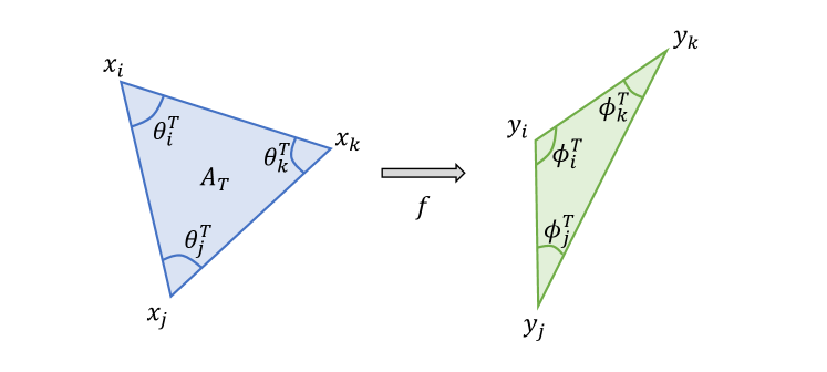
Figure 1: A figure illustrating the geometric distortion of a triangle $T$ under mapping $f$.

Theorem 5.7.

Under the above notations, suppose the length of all the edges in $(\mathcal{X},\mathcal{T})$ are less than $R$, $\lambda^{true}_{ij}<\Lambda^{t}$ and $\lambda_{ij}>\lambda_{0}$ for any $i,j$, where $0<\lambda_{0}<\Lambda^{t}$, denote $r_{\lambda}=\Lambda^{t}/\lambda_{0}$, then

(56) $$\begin{split}&\quad\left(\frac{e^{\eta^{2}r^{2}_{\lambda}R^{2}}}{\eta^{2}}\right)^{2}D_{\sigma}+\frac{84|\mathcal{T}|}{N^{2}}r^{4}_{\lambda}R^{4}\\ &\geq\frac{4}{\pi^{2}}\frac{1}{N^{2}}\sum_{\{i,j,k\}=T\in\mathcal{T}}A_{T}^{2}\left[\left(\theta^{T}_{i}-\phi^{T}_{i}\right)^{2}+\left(\theta^{T}_{j}-\phi^{T}_{j}\right)^{2}+\left(\theta^{T}_{k}-\phi^{T}_{k}\right)^{2}\right]\end{split}$$

where $A_{T}$ is the area of triangle formed by $x_{i},x_{j},x_{k}$, $\theta^{T}_{i}=\angle x_{k}x_{i}x_{j},\phi^{T}_{i}=\angle y_{k}y_{i}y_{j}$.

Proof 5.8.

Write $d^{x}_{ij}=\|x_{i}-x_{j}\|,d^{y}_{ij}=\|y_{i}-y_{j}\|$, $\eta=1/\sigma$. By MVT, for $a<b$, there exists $c\in(a,b)$ such that

(57) $$\begin{split}e^{-\eta^{2}b}-e^{-\eta^{2}a}&=-\eta^{2}e^{-c}(b-a)\\ (e^{-\eta^{2}b}-e^{-\eta^{2}a})^{2}&\geq(\eta^{2}e^{-\eta^{2}\max(a,b)})^{2}(b-a)^{2}.\end{split}$$

Then

(58) $$\begin{split}D_{ij}&=\left(e^{-(d^{x}_{ij})^{2}/\sigma^{2}}-e^{-(d^{y}_{ij})^{2}/\sigma^{2}\lambda_{ij}^{2}}\right)^{2}\\ &\geq\left((d^{x}_{ij})^{2}-(d^{y}_{ij})^{2}/\lambda_{ij}^{2}\right)^{2}\left(\eta^{2}e^{-\eta^{2}\max\{(d^{x}_{ij})^{2},(d^{y}_{ij})^{2}/\lambda_{ij}^{2}\}}\right)^{2}\\ &\geq\left((d^{x}_{ij})^{2}-(d^{y}_{ij})^{2}/\lambda_{ij}^{2}\right)^{2}\left(\eta^{2}e^{-\eta^{2}r^{2}_{\lambda}(d^{x}_{ij})^{2}}\right)^{2},\end{split}$$

as by definition,

(59) $$r_{\lambda}=\frac{\Lambda^{t}}{\lambda_{0}}>\max\left\{1,\frac{d^{y}_{ij}}{d^{x}_{ij}\lambda_{ij}}\right\}.$$

Pick $T=\{i,j,k\}\in\mathcal{T}$. For simpler notations, write the edge representations $e^{T}_{1}=[ij]$, $e^{T}_{2}=[jk]$, $e^{T}_{3}=[ki]$, with a period of $3$, i.e. $e^{T}_{n}=e^{T}_{n+3}$. Since $a^{2}+b^{2}+c^{2}=\frac{1}{4}(a+b+c)^{2}+\frac{1}{4}(a+b-c)^{2}+\frac{1}{4}(a-b+c)^{2}+\frac{1}{4}(a-b-c)^{2}$ ,

(60) $$\begin{split}&\quad D_{ij}+D_{jk}+D_{ki}=D_{e^{T}_{1}}+D_{e^{T}_{2}}+D_{e^{T}_{3}}\\ &\geq\sum_{n=1}^{3}\left((d^{x}_{e^{T}_{n}})^{2}-(d^{y}_{e^{T}_{n}})^{2}/\lambda_{e^{T}_{n}}^{2}\right)^{2}\left(\eta^{2}e^{-\eta^{2}r^{2}_{\lambda}\left(d^{x}_{e^{T}_{n}}\right)^{2}}\right)^{2}\\ &\geq\left(\eta^{2}e^{-\eta^{2}r^{2}_{\lambda}R^{2}}\right)^{2}\sum^{3}_{n=1}\left((d^{x}_{e^{T}_{n}})^{2}-(d^{y}_{e^{T}_{n}})^{2}/\lambda_{e^{T}_{n}}^{2}\right)^{2}\\ &\geq\frac{1}{4}\left(\eta^{2}e^{-\eta^{2}r^{2}_{\lambda}R^{2}}\right)^{2}\sum^{3}_{n=1}\left[\sum^{2}_{m=0}(-1)^{m}\left(\left(d^{x}_{e^{T}_{n+m}}\right)^{2}-\left(d^{y}_{e^{T}_{n+m}}\right)^{2}/\left(\lambda_{e^{T}_{n+m}}^{2}\right)\right)\right]^{2}\end{split}$$

Below, consider only the terms with $n=2$ in the last inequality of (60), and the others follow directly by symmetry.

Define points $y^{\prime}_{i},y^{\prime}_{k}$ such that $y_{j},y_{i},y^{\prime}_{i}$ are collinear, and $y_{j},y_{k},y^{\prime}_{k}$ are collinear, and $\|y^{\prime}_{i}-y_{j}\|=d^{y}_{ij}/\lambda_{ij}$, $\|y^{\prime}_{k}-y_{j}\|=d^{y}_{jk}/\lambda_{jk}$. Denote $\theta_{j}=\angle x_{i}x_{j}x_{k},d^{\prime}_{ij}=\|y^{\prime}_{i}-y^{\prime}_{j}\|,\phi_{j}=\angle y_{i}y_{j}y_{k}=\angle y^{\prime}_{i}y_{j}y^{\prime}_{k}$.

Apply law of cosines to the triangles formed by $x_{i},x_{j},x_{k}$ and $y^{\prime}_{i},y_{j},y^{\prime}_{k}$,

(61) $$\begin{split}&\quad\left((d^{x}_{ij})^{2}-(d^{y}_{ij})^{2}/\lambda_{ij}^{2}\right)+\left((d^{x}_{jk})^{2}-(d^{y}_{jk})^{2}/\lambda_{jk}^{2}\right)-\left((d^{x}_{ki})^{2}-(d^{y}_{ki})^{2}/\lambda_{ki}^{2}\right)\\ &=[2d^{x}_{ij}d^{x}_{jk}\cos\theta_{j}]-[(d^{y}_{ij})^{2}/\lambda_{ij}^{2}+(d^{y}_{jk})^{2}/\lambda_{jk}^{2}-(d^{\prime}_{ik})^{2}]-[(d^{\prime}_{ik})^{2}-(d^{y}_{ki})^{2}/\lambda_{ki}^{2}]\\ &=2d^{x}_{ij}d^{x}_{jk}\cos\theta_{j}-2d^{y}_{ij}d^{y}_{jk}/\lambda_{ij}\lambda_{jk}\cos\phi_{j}-[(d^{\prime}_{ik})^{2}-(d^{y}_{ki})^{2}/\lambda_{ki}^{2}]\\ &=2d^{x}_{ij}d^{x}_{jk}\left(\cos\theta_{j}-\frac{\lambda_{ij}^{true}\lambda_{jk}^{true}}{\lambda_{ij}\lambda_{jk}}\cos\phi_{j}\right)-[(d^{\prime}_{ik})^{2}-(d^{y}_{ki})^{2}/\lambda_{ki}^{2}]\\ &=2d^{x}_{ij}d^{x}_{jk}\left[\cos\theta_{j}-\cos\phi_{j}\right]+2d^{x}_{ij}d^{x}_{jk}\cos\phi_{j}\left[1-\frac{\lambda_{ij}^{true}\lambda_{jk}^{true}}{\lambda_{ij}\lambda_{jk}}\right]+\left[(d^{y}_{ki})^{2}/\lambda_{ki}^{2}-(d^{\prime}_{ik})^{2}\right].\end{split}$$

By mean value theorem, there exists some angle $\psi$ between $\theta$ and $\phi$ such that

(62) $$\begin{split}\cos\theta-\cos\phi&=-\sin\psi(\theta-\phi)\\ (\cos\theta-\cos\phi)^{2}&=\sin^{2}\psi(\theta-\phi)^{2}.\\ \end{split}$$

If $\theta=\phi$, take $\psi=\theta$. If not,

(63) $$\begin{split}\sin^{2}\psi&=\frac{(\cos\theta-\cos\phi)^{2}}{(\theta-\phi)^{2}}=\frac{\sin^{2}\frac{\theta+\phi}{2}\sin^{2}\frac{\theta-\phi}{2}}{\left(\frac{\theta-\phi}{2}\right)^{2}}.\end{split}$$

If $\theta\neq\phi$, since $0<\theta,\phi<\pi$, $-\frac{\pi}{2}<\frac{\theta-\phi}{2}<\frac{\pi}{2}$, $\frac{2}{\pi}<\frac{\sin\frac{\theta-\phi}{2}}{\frac{\theta-\phi}{2}}<1$, then:

(64) $$\begin{split}\sin^{2}\psi&>\frac{4}{\pi^{2}}\sin^{2}\frac{\theta+\phi}{2}\geq\frac{1}{\pi^{2}}(\sin\theta+\sin\phi)^{2}.\\ \end{split}$$

So,

(65) $$\begin{split}(\cos\theta-\cos\phi)^{2}>\frac{1}{\pi^{2}}(\sin\theta+\sin\phi)^{2}(\theta-\phi)^{2},\\ \end{split}$$

and since $0<\phi<\pi$,

(66) $$\begin{split}(\cos\theta-\cos\phi)^{2}>\frac{1}{\pi^{2}}\sin^{2}\theta(\theta-\phi)^{2}.\\ \end{split}$$

Note the three terms in 61 are bounded:

(67) $$\begin{split}\left|2d^{x}_{ij}d^{x}_{jk}\left[\cos\theta_{j}-\cos\phi_{j}\right]\right|\leq 4R^{2},\end{split}$$

(68) $$\begin{split}\left|2d^{x}_{ij}d^{x}_{jk}\cos\phi_{j}\left[1-\frac{\lambda_{ij}^{true}\lambda_{jk}^{true}}{\lambda_{ij}\lambda_{jk}}\right]\right|\leq 2R^{2}\left[1+r_{\lambda}^{2}\right],\end{split}$$

(69) $$\begin{split}&\quad\left|(d^{y}_{ki})^{2}/\lambda_{ki}^{2}-(d^{\prime}_{ik})^{2}\right|\\ &\leq(d^{x}_{ki})^{2}(\lambda^{true}_{ki})^{2}/\lambda_{ki}^{2}+(d^{\prime}_{ij}+d^{\prime}_{jk})^{2}\\ &\leq R^{2}r_{\lambda}^{2}+(d^{x}_{ij}\lambda^{true}_{ij}/\lambda_{ij}+d^{x}_{jk}\lambda^{true}_{jk}/\lambda_{jk})^{2}\\ &=5R^{2}r_{\lambda}^{2},\\ \end{split}$$

and $(a+b+c)^{2}+C\geq a^{2}+b^{2}+c^{2}$ if $C\geq 2|ab|+2|bc|+2|ca|$.

As a result,

(70) $$\begin{split}&\quad\left[\left((d^{x}_{ij})^{2}-(d^{y}_{ij})^{2}/\lambda_{ij}^{2}\right)+\left((d^{x}_{jk})^{2}-(d^{y}_{jk})^{2}/\lambda_{jk}^{2}\right)-\left((d^{x}_{ki})^{2}-(d^{y}_{ki})^{2}/\lambda_{ki}^{2}\right)\right]^{2}+C\\ &=\Bigg{[}2d^{x}_{ij}d^{x}_{jk}\left[\cos\theta_{j}-\cos\phi_{j}\right]+2d^{x}_{ij}d^{x}_{jk}\cos\phi_{j}\left[1-\frac{\lambda_{ij}^{true}\lambda_{jk}^{true}}{\lambda_{ij}\lambda_{jk}}\right]\\ &\quad+\left[(d^{y}_{ki})^{2}/\lambda_{ki}^{2}-(d^{\prime}_{ik})^{2}\right]\Bigg{]}^{2}+C\\ &\geq\left(2d^{x}_{ij}d^{x}_{jk}\right)^{2}\left[\cos\theta_{j}-\cos\phi_{j}\right]^{2}+\left[2d^{x}_{ij}d^{x}_{jk}\cos\phi_{j}\right]^{2}\left[1-\frac{\lambda_{ij}^{true}\lambda_{jk}^{true}}{\lambda_{ij}\lambda_{jk}}\right]^{2}\\ &\quad+\left[(d^{y}_{ki})^{2}/\lambda_{ki}^{2}-(d^{\prime}_{ik})^{2}\right]^{2}\\ &\geq\frac{4}{\pi^{2}}\left(d^{x}_{ij}d^{x}_{jk}\sin\theta_{j}\right)^{2}\left(\theta_{j}-\phi_{j}\right)^{2}+\left[2d^{x}_{ij}d^{x}_{jk}\cos\phi_{j}\right]^{2}\left[1-\frac{\lambda_{ij}^{true}\lambda_{jk}^{true}}{\lambda_{ij}\lambda_{jk}}\right]^{2}\\ &\quad+\left[(d^{y}_{ki})^{2}/\lambda_{ki}^{2}-(d^{\prime}_{ik})^{2}\right]^{2}\\ &\geq\frac{16}{\pi^{2}}A_{ijk}^{2}\left(\theta_{j}-\phi_{j}\right)^{2}+\left[2d^{x}_{ij}d^{x}_{jk}\cos\phi_{j}\right]^{2}\left[1-\frac{\lambda_{ij}^{true}\lambda_{jk}^{true}}{\lambda_{ij}\lambda_{jk}}\right]^{2}+\left[(d^{y}_{ki})^{2}/\lambda_{ki}^{2}-(d^{\prime}_{ik})^{2}\right]^{2},\end{split}$$

where

(71) $$\begin{split}C&=112R^{4}r_{\lambda}^{4}\\ &\geq 16R^{4}\left[1+r_{\lambda}^{2}\right]+20R^{4}\left[1+r_{\lambda}^{2}\right]r_{\lambda}^{2}+40R^{4}r_{\lambda}^{2}\\ &=R^{4}\left(16+76r^{2}_{\lambda}+20r^{4}_{\lambda}\right),\end{split}$$

and $A_{ijk}$ is the area of triangle $x_{i},x_{j},x_{k}$.

So the inequality (60) becomes:

(72) $$\begin{split}&\quad\sum_{n=1}^{3}D_{e^{T}_{n}}+84\left(\eta^{2}r^{2}_{\lambda}R^{2}e^{-\eta^{2}r^{2}_{\lambda}R^{2}}\right)^{2}\\ &=\sum_{n=1}^{3}D_{e^{T}_{n}}+\frac{1}{4}\left(\eta^{2}e^{-\eta^{2}r^{2}_{\lambda}R^{2}}\right)^{2}(3C)\\ &\geq\frac{1}{4}\left(\eta^{2}e^{-\eta^{2}r^{2}_{\lambda}R^{2}}\right)^{2}\sum^{3}_{n=1}\left[\sum^{2}_{m=0}(-1)^{m}\left(\left(d^{x}_{e^{T}_{n+m}}\right)^{2}-\left(d^{y}_{e^{T}_{n+m}}\right)^{2}/\left(\lambda_{e^{T}_{n+m}}^{2}\right)\right)\right]^{2}+C\\ &\geq\frac{4}{\pi^{2}}A_{ijk}^{2}\left(\eta^{2}e^{-\eta^{2}r^{2}_{\lambda}R^{2}}\right)^{2}\left[\left(\theta_{j}-\phi_{j}\right)^{2}+\left(\theta_{i}-\phi_{i}\right)^{2}+\left(\theta_{k}-\phi_{k}\right)^{2}\right].\end{split}$$

Now, an inequality relates the energy and angle distortion on one triangle is obtained.

(73) $$\begin{split}D_{\sigma}=\sum_{i,j=1}^{N}D_{ij}\geq\sum_{T\in\mathcal{T}}\sum_{n=1}^{3}D_{e^{T}_{n}},\end{split}$$

and,

(74) $$\begin{split}&\quad\left(\frac{e^{\eta^{2}r^{2}_{\lambda}R^{2}}}{\eta^{2}}\right)^{2}D_{\sigma}+\frac{84|\mathcal{T}|}{N^{2}}r^{4}_{\lambda}R^{4}\\ &\geq\frac{1}{N^{2}}\sum_{\{i,j,k\}=T\in\mathcal{T}}\left(\frac{e^{\eta^{2}r^{2}_{\lambda}R^{2}}}{\eta^{2}}\right)^{2}\left[D_{ij}+D_{jk}+D_{ki}+84\left(\eta^{2}r^{2}_{\lambda}R^{2}e^{-\eta^{2}r^{2}_{\lambda}R^{2}}\right)^{2}\right]\\ &\geq\frac{4}{\pi^{2}}\frac{1}{N^{2}}\sum_{\{i,j,k\}=T\in\mathcal{T}}A_{T}^{2}\left[\left(\theta^{T}_{i}-\phi^{T}_{i}\right)^{2}+\left(\theta^{T}_{j}-\phi^{T}_{j}\right)^{2}+\left(\theta^{T}_{k}-\phi^{T}_{k}\right)^{2}\right]\\ &\quad+(\text{regularity terms}),\end{split}$$

and the desired inequality is obtained.

The term $e^{\eta^{2}r^{2}_{\lambda}R^{2}}/\eta^{2}$ attains minimum when $\sigma=1/\eta=r_{\lambda}R$ and its minimum value is $r^{2}_{\lambda}R^{2}e$. Together with the second terms $\frac{84|\mathcal{T}|}{N^{2}}r^{4}_{\lambda}R^{4}$, the inequality, the theorem stated above suggests that a proper choice of $\sigma$ and a small value of $r_{\lambda}R$ provide an better upper bound for the angle distortions between the original point cloud and its mapping. While the factor $r_{\lambda}$ is related to the mapping obtained in the optimization process, the factor $R$ is related to the assumed mesh structure. If we assume a mesh structure that is better describing the underlying surface, a smaller $R$ can be obtained. An illustration to the idea is shown in Figure 2. Also, the theorem has no assumptions on the surface topology. Angle distortion from multiply-connected surfaces or surfaces with multiple components can be controlled through minimizing LEG $D_{\sigma}$.

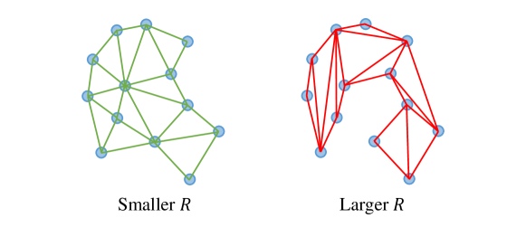
Figure 2: An illustration to how different mesh structure on the same point cloud affect $R$.

5.3 Optimization Algorithm

With the discussed loss functions, we model the surface parametrization problem as a optimization problem, with three terms: LEG, HAND for parameter domain matching, and HAND for landmark matching,

(75) $$f,\lambda=\operatorname*{argmin}_{f,\lambda}\beta_{1}D_{\sigma}(f,\lambda,\mathcal{X})+\beta_{2}H_{\alpha}(f(\mathcal{X}),\mathcal{W})+\beta_{3}\sum_{k=1}^{M}H_{\alpha}\left(f(\mathcal{P}_{k}),\mathcal{Q}_{k}\right)$$

where $\beta_{1},\beta_{2}>0,\beta_{3}$, $\mathcal{X}\subseteq\mathcal{M}$ is the point cloud surface, $\mathcal{W}\subseteq\Omega$ is a set of finite points in the parameter domain, $\{\mathcal{P}_{k}\}_{k=1}^{M}$ and $\{\mathcal{Q}_{k}\}_{k=1}^{M}$ are landmark and target finite point sets. Also, in order to better regularize the geometry of the neighbourhood of the landmarks, the landmarks are included in the calculation of LEG. The symmetric bivariate function $\lambda:\mathcal{X}\times\mathcal{X}\to\mathbb{R}$ is represented as a univariate function $\lambda_{inv}$ by $1/\lambda(x_{i},x_{j})=\lambda_{inv}(x_{i})+\lambda_{inv}(x_{j})$, which is named inverse $\lambda$ function. The optimization problem 75 is finalized as

(76) $$\begin{split}&\quad f,\lambda_{inv}=\operatorname*{argmin}_{f,\lambda_{inv}}\mathcal{L}(f,\lambda_{inv},\mathcal{X},\mathcal{W},\{\mathcal{P}_{k}\}_{k=1}^{M},\{\mathcal{Q}_{k}\}_{k=1}^{M})\\ &=\operatorname*{argmin}_{f,\lambda_{inv}}\beta_{1}D_{\sigma}\left(f,\lambda_{inv},\mathcal{X}\cup\mathcal{P}\right)+\beta_{2}H_{\alpha}(f(\mathcal{X}),\mathcal{W})+\beta_{3}\sum_{k=1}^{M}H_{\alpha}\left(f(\mathcal{P}_{k}),\mathcal{Q}_{k}\right),\end{split}$$

where $\mathcal{P}=\bigcup_{k=1}^{M}\mathcal{P}_{k}$.

For the sake of continuity, we represent the mapping function and inverse $\lambda$ function using neural networks, giving the names parametrization net and inverse $\lambda$ net. Stochastic gradient descent (SGD) is also applied in the optimization. By the traditional idea of SGD, in $i$-epoch and $j$-batch, we sample subsets $\mathcal{X}^{i,j}\subseteq\mathcal{X}$ and $\mathcal{W}^{i,j}\subseteq\mathcal{W}$, and compute gradient of

(77) $$\mathcal{L}^{i,j}=\mathcal{L}(f,\lambda_{inv},\mathcal{X}^{i,j},\mathcal{W}^{i,j},\{\mathcal{P}_{k}\}_{k=1}^{M},\{\mathcal{Q}_{k}\}_{k=1}^{M}),$$

for updates in SGD. Here the landmarks and targets are not subsampled, as they have much smaller sizes compared to the point cloud $\mathcal{X}$ in general.

Apart from the traditional meaning of approximation to the full gradient, the Theorems 5.3 and 5.7 proved previously provide a geometrical view for applying SGD. The point set $\mathcal{X}^{i,j}\cup\mathcal{P}$ can also be understood as a point cloud of the underlying surface $\mathcal{M}$, coarser than $\mathcal{X}$. The term $D_{\sigma}(f,\lambda_{inv},\mathcal{X}^{i,j}\cup\mathcal{P})$ is not only an approximation to $D_{\sigma}(f,\lambda_{inv},\mathcal{X}\cup\mathcal{P})$, but also a measurement of geometric distortion of the coarsened point cloud under mapping $f$. Theorem 5.7 suggests that minimization on $D_{\sigma}(f,\lambda_{inv},\mathcal{X}^{i,j}\cup\mathcal{P})$ reduces the angle distortion of an underlying surface mesh on $\mathcal{X}^{i,j}\cup\mathcal{P}$. On the other hand, by Theorem 5.3, $H_{\alpha}(f(\mathcal{X}^{i,j}),\mathcal{W}^{i,j})$ measures the alignment between the mapping $f(\mathcal{X}^{i,j})$ and point set $\mathcal{W}^{i,j}$. Moreover, the two theorems also suggest that the performance of surface parametrization can be improved, in the sense of Hausdorff distance and angle distortion, by increasing the batch size.

By design, the whole optimization process is divided into different stages, where the batch size is doubled after each stage, until the whole point cloud $\mathcal{X}$ is used. Denote the number of epochs to be $E$, and the batch size to be $B_{\mathcal{X}}$ and $B_{\mathcal{W}}$. The number of mini-batches in an epoch is set to be $B=\lceil|\mathcal{X}|/B_{\mathcal{X}}\rceil$. The computation of loss functions requires around $B_{\mathcal{X}}^{2}+B_{\mathcal{X}}\cdot B_{\mathcal{W}}$ pairwise distances. Therefore the overall computation in a stage requires $E\cdot B\cdot(B_{\mathcal{X}}^{2}+B_{\mathcal{X}}\cdot B_{\mathcal{W}})\approx E\cdot|\mathcal{X}|\cdot(B_{\mathcal{X}}+B_{\mathcal{W}})$ pairs of distances. To compensate the rise in computations caused by doubling the batch size, the number of epochs is halved after each stage. This setting can be intuitively understood as fitting general pattern using coarser point clouds at first, then fine-tuning the details using the whole point cloud. The idea of this mechanism is illustrated in figure 3.

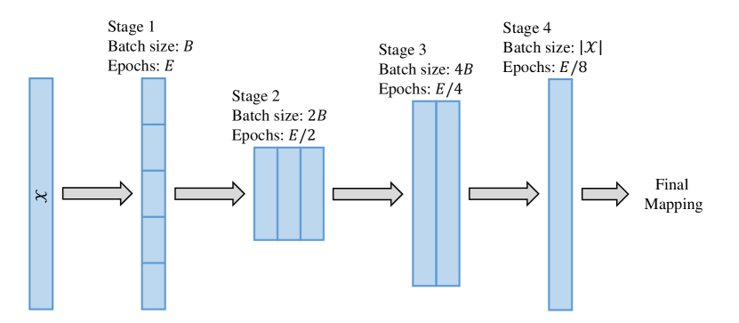
Figure 3: An illustration to the dynamics of the suggested optimization algorithm.

In the theorem 5.7, we observe that the optimal choice of $\sigma$ depends on $R$ and $r_{\lambda}$. When the density of the point cloud increases, the gaps between the points shrink. If the batch size is doubled in each stage, then $R$, the longest edge length, is expected to scale down to $R/\sqrt{2}$. Therefore, the parameter $\sigma$ is also scaled to $\sigma/\sqrt{2}$ to match $R$. Moreover, Theorem 5.3 states the importance of a large choice of $\alpha$, and so the values of $\alpha$ is also doubled after each stage. In practice, the increment of $\alpha$ is done by a linear increase, from $\alpha_{initial}$ at the stage of a stage, to the desired values $\alpha_{final}$. Depending on the number of stages, parameters may become too extreme, leading to numerical instability. In our algorithm, capping the values of $\alpha,\sigma$, and also the number of epochs, are performed to avoid the potential problems.

The discussed optimization algorithm is summarized in Algorithm 1 .

Algorithm 1 Optimization Scheme

1:Data: a point cloud $\mathcal{X}$, point set from parameter domain $\mathcal{W}$, landmark points $\{\mathcal{P}_{k}\}_{k=1}^{M}$ and targets $\{\mathcal{Q}_{k}\}_{k=1}^{M}$ ; Loss function weightings: $\beta_{1}$, $\beta_{2}$, $\beta_{3}$ ; Initial training hyperparameters: number of epochs $E$, batch sizes $B_{\mathcal{X}}$ and $B_{\mathcal{W}}$; LEG parameter $\sigma$ ; HAND parameters, $\alpha_{initial}$, $\alpha_{final}$ ; Parameter bounds: $\sigma_{min}$, $\alpha_{max}$, $E_{min}$.

2:Trained parametrization net $f$ and inverse $\lambda$-Net $\lambda$.

3:Initialize networks $f$, $\lambda_{inv}$;

4:$continue$ $\leftarrow$ $True$;

5:while  $continue$  do

6:  if $B_{\mathcal{X}}=|\mathcal{X}|$ then

7:   $continue$ $\leftarrow$ $False$;

8:  end if

9:  $\alpha\leftarrow\alpha_{inital}$;

10:  for $i=1,\cdots,E$ do

11:   for $j=1,\cdots,\lceil|\mathcal{X}|/B_{\mathcal{X}}\rceil$ do

12:     Sample $B_{\mathcal{X}}$ points from $\mathcal{X}$, form $\mathcal{X}^{i,j}$;

13:     Sample $B_{\mathcal{W}}$ points from $\mathcal{W}$, form $\mathcal{W}^{i,j}$ ;

14:     Compute $\mathcal{L}^{i,j}$ in 77 and its gradient;

15:     Update $f,\lambda_{inv}$ ;

16:   end for

17:   if $i<E$ then

18:     $\alpha\leftarrow\alpha+(\alpha_{final}-\alpha_{initial})/(E-1)$ ;

19:   end if

20:  end for

21:  $\sigma\leftarrow\max(\sigma/\sqrt{2},\sigma_{min})$;

22:  $\alpha_{initial}\leftarrow\alpha_{final}$;

23:  $\alpha_{final}\leftarrow\min(2\alpha_{final},\alpha_{max})$;

24:  $E\leftarrow\max(E/2,E_{min})$;

25:  $B_{\mathcal{X}}\leftarrow\min(2B_{\mathcal{X}},|\mathcal{X}|)$;

26:  $B_{\mathcal{W}}\leftarrow\min(2B_{\mathcal{W}},|\mathcal{W}|)$;

27:end while

6 Implementation

The proposed loss functions and optimization algorithm were implemented in Python, using deep learning library PyTorch [50]. The experiments were computed using an NVIDIA RTX A6000.

The parameters used in the algorithm are stated here. If the associated loss function is used, LEG weight $\beta_{1}=5$, HAND weight $\beta_{2}=1$ for matching parameter domain, landmark mismatch energy weight $\beta_{3}=1$. At the beginning of the first stage in the optimization process, number of epochs $E=10000$, batch sizes $B_{\mathcal{X}}=B_{\mathcal{W}}=1024$, LEG parameter $\sigma=0.5$, HAND parameters $\alpha_{initial}=2$, $\alpha_{final}=20$. We bound the parameters by $\sigma_{min}=0.001$, $\alpha_{max}=100$, $E_{min}=1000$.

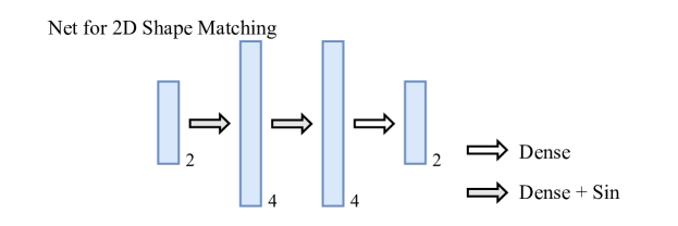
Figure 4: Architecture of the parametrization net used in shape matching. The arrows indicate the forward process. The bars indicate the latent variables, with dimensions stated under them.

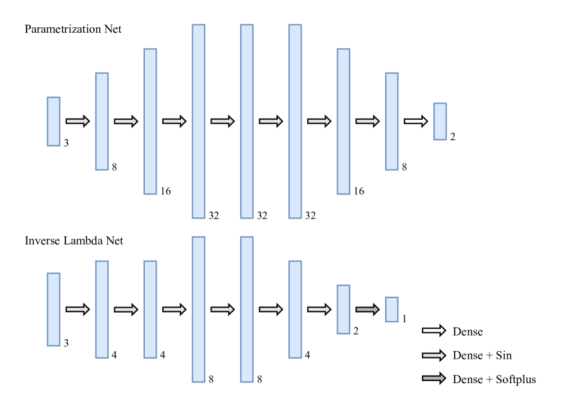
Figure 5: Architecture of the parametrization and $\lambda_{inv}$ nets. The arrows indicate the forward process. The bars indicate the latent variables, with dimensions stated under them.

Networks of difference sizes are used for varying levels of difficulty. For the experiments on shape matching, we use the parametrization networks with simple architecture shown in Figure 4 and no $\lambda_{inv}$ net is involved. The other experiments use larger fully-connected neural networks to model the parametrization functions and $\lambda_{inv}$ functions, with architecture shown in Figure 5. In the networks, the sine function is used as the activation, except for the output layers. No activation is needed for parametrization nets, while the softplus function is used to activate the last layer of the $\lambda_{inv}$ nets so that the output is always positive. The minimization is done by stochastic gradient descent with RMSprop [58] with parameters $\alpha=0.99$, a learning rate of $0.0001$, with a momentum of $0.9$. All the weights and biases in the networks are randomly initialized, and hence the initial mappings and $\lambda_{inv}$ values.

7 Experimental results

In this section, we illustrate the performance of our proposed methods through experiments conducted with various combinations of loss function terms, each serving different purposes. Additionally, different parameter domains, including various shapes and topologies, are used in experiments to demonstrate the flexibility of our methods.

Due to the challenges of collecting point cloud data, the point cloud surfaces used in our study are the vertices of triangular meshes. To numerically demonstrate the performance of our methods, we measured the Hausdorff distance and angle distortion in our experiments. Specifically, the Hausdorff distance is measured between the mapped point cloud and a densely and uniformly sampled finite point set in the parameter domain. The angle distortion is calculated as the difference between the angles of the original triangular mesh and its mapping.

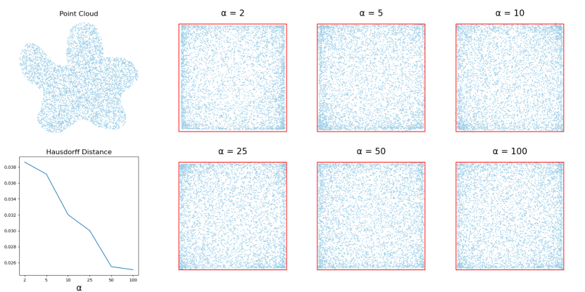
Figure 6: The mappings obtained by minimizing HAND with $\alpha=2,5,10,25,50,100$ on a 2D point cloud and a plot of their Hausdorff distance to a square, with boundary drawn in red.

We begin with an experiment for 2D shape matching using only the proposed Hausdorff Approximation from Node-wise Distances (HAND), utilizing the neural networks architecture illustrated in Figure 4. The experimental results are shown in Figure 6. A point cloud in an irregular shape, with $5000$ points in $\mathbb{R}^{2}$ is created, and mapped to a unit square. The boundary is drawn in red lines, using only the presence of HAND, without considering the geometry distortion. We test the performance of HAND with different parameters $\alpha=2,5,10,25,50,100$. Due to the simplicity of the task, the optimizations are performed directly on entire point cloud, without dividing the optimization into several stages as discussed in Section 5.3. The ability of shape matching by minimizing HAND is demonstrated in the Figure 6. Moreover, as value of $\alpha$ increases, a better match between the point cloud mapping and the boundary of the square is shown. Along with the line plot illustrating a decreasing trend in the Hausdorff distance as $\alpha$ increases, we can conclude that a larger value of $\alpha$ improves the performance of HAND in terms of matching matching the parameter domain.

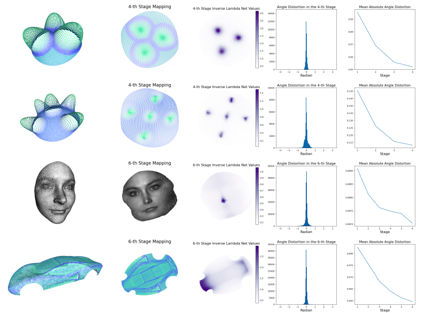
Figure 7: The results of free boundary experiments obtained by minimizing only LEG. Each row represent an experimental result for an input surface. Top to bottom: three spikes, five spikes, human face, car surface. Left to right: the input point cloud surface, final stage mapping, final stage inverse $\lambda$-Net values, histogram for angle distortion (in radian), and line plot of mean absolute angle distortion (in radian) against stages.

After demonstrating the shape matching capability, the rest of this section presents the parametrization experiments using the neural networks shown in Figure 5.

Experiments on free-boundary parametrization, which minimized only Localized Energy for Geometry (LEG), for surface point clouds, are presented. We examine two open surfaces, one with three peaks and another with five peaks, both containing $5809$ points, and $11366$ faces in the original triangular meshes. Additionally, a human face mesh with $24891$ points and $49272$ faces, as well as a car surface with $19320$ points and $38057$ faces, are included in the free-boundary parametrization experiments.

The parametrization results are illustrated in Figure 7. Figure 7 shows the outputs of the parametrization networks $f(\mathcal{X})$ and inverse $\lambda$ networks $\lambda_{inv}(\mathcal{X})$ at the last stage. The histograms, which indicate that the angle differences in the last stage are concentrated at 0, suggest the ability of angle preserving via minimization of LEG. Also, the line plots illustrate decreasing trends in mean absolute angle distortion with the progression of stages, demonstrating that the optimization scheme yields better parametrization results. The plots for $\lambda_{inv}(\mathcal{X})$ show that if the points are concentrated in certain regions, for example the peaks, nose, or the front part of the car shown in Figure 7, the output values of $\lambda_{inv}$ nets are higher. This observation aligns with the intuition that $\lambda_{inv}$ measures the scaling of distance under the mapping $f$, and confirms the significance of $\lambda_{inv}$.

Next, experiments are conducted by incorporating both HAND and LEG in the optimization process. The human face and car surface used previously in free-boundary parametrization experiments are also used in the following experiments.

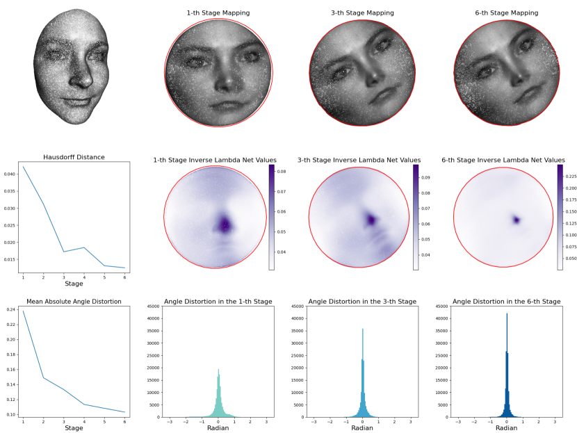
Figure 8: Results for parametrizing a human face to unit disk. In the first column, the input human face, line plot for Hausdorff distance against stages, line plot for mean absolute angle distortion (in radian) are plotted from top to bottom. The second to the last columns show the result after the $1^{\text{st}}$, $3^{\text{rd}}$ and $6^{\text{th}}$ stages, including output mappings, $\lambda_{inv}$ networks output values, histogram for angle distortion (in radian) from top to bottom. The red lines indicate the boundary of the unit disk.

First of all, the parametrization on the human face is computed, with a unit disk chosen as the target parameter domain. The experimental results are shown in Figure 8. This figure summarizes the overall performance of parametrization using the two line plots: one showing Hausdorff distance, the other showing mean absolute angle distortion (in radian), against stages. The plots generally show decreasing trends, suggesting the improvements made during the optimization process through parameter adjustments. The evolution from the earlier stages to latter stages are shown by plotting the results after the $1^{\text{st}}$, $3^{\text{rd}}$ and $6^{\text{th}}$ stages, with details in the last three columns. In the $1^{\text{st}}$ stage, a gap between the point cloud mapping and the boundary of the parameter domain can be clearly observed. Meanwhile, the alignment between the mapping and boundary is much better improved in latter stages, supporting the line plot for Hausdorff distance. The histograms for angle distortion (in radian) illustrate that the angle distortion are more concentrated at 0 in the latter stages than in the earlier stages, coinciding with the decrease in mean absolute angle distortion shown in the line plot. We can also observe that the mapping of the nose shrinks as the stages progress, matching the rising values in the nose illustrated in the plots for $\lambda_{inv}$ values.

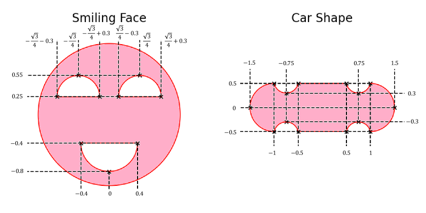
Figure 9: The smiling face and car shape used as parameter domains. The horizontal dash lines are indicating the $y$-coordinates of the points on the lines, and the $x$-coordinates are indicated by the vertical dash lines.

Instead of choosing a simple parameter domain such as a unit disk, experiments with more complicated parameter domains are demonstrated. The human face point cloud, used in the previous experiment, with its mouth and two eyes removed, is mapped to a multiply-connected smiling face. This face is created by removing three smaller half-disks from the unit disk and is shown on the left of Figure 9. Also, a car surface point cloud is mapped to a car-shaped parameter domain, whose boundary consist of circular arcs and straight lines, as shown on the right of Figure 9. Figure 9, which illustrates the mentioned parameter domain, also indicates the coordinates for some important points in the shapes. The horizontal dash lines indicate the $y$-coordinates, while vertical dash lines indicate the $x$-coordinates.

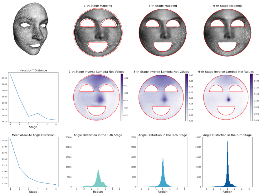
Figure 10: Results for parametrizing a human face, with its mouth and eyes removed, to a prescribed smiling face. In the first column, the input human face, line plot for Hausdorff distance against stages, line plot for mean absolute angle distortion (in radian) are plotted from top to bottom. The second to the last columns show the result after the $1^{\text{st}}$, $3^{\text{rd}}$ and $6^{\text{th}}$ stages, including output mappings, $\lambda_{inv}$ networks output values, histogram for angle distortion (in radian) from top to bottom. The red lines indicate the boundaries of the smiling face.

Mouth and eyes are removed from the previously used human face, resulting in a triangular mesh with $23871$ points and $46973$ faces. Its vertices are used as an input point cloud surface in computing a parametrization to the smiling face drawn in Figure 9. The experimental results are shown below in Figure 10. The plots in the figure are similar to the above experiment, which parametrized the simply-connected human face to the unit disk. By observing the point cloud mappings and histograms for angle distortion, we can see the mismatch between the point cloud mapping and high angle distortion appeared in the earlier stages, while they are greatly improved in the latter stages. This provides evidence to the decreasing trends shown in the two line plots for Hausdorff distance and mean absolute angle distortion against stages. The changes in $\lambda_{inv}$ values also reflect the changes in the scaling of the mappings.

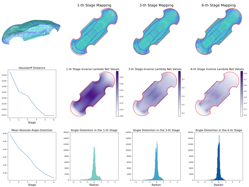
Figure 11: Results for parametrizing a car surface, to a prescribed car shape domain. In the first column, the input human face, line plot for Hausdorff distance against stages, line plot for mean absolute angle distortion (in radian) are plotted from top to bottom. The second to the last columns show the result after the $1^{\text{st}}$, $3^{\text{rd}}$ and $6^{\text{th}}$ stages, including output mappings, $\lambda_{inv}$ networks output values, histogram for angle distortion (in radian) from top to bottom. The red lines indicate the boundary of the car shape. The mappings and $\lambda_{inv}$ plots are rotated $45^{\circ}$.

In Figure 11, a point cloud sampled from the outer shell of a car surface, drawn in the upper left corner, is used and mapped to the prescribed car-shaped parameter domain shown in Figure 9. The other plots include Hausdorff distance, mean absolute angle distortion, and the mappings, $\lambda_{inv}$ and histograms for angle distortion. The plots for mappings and $\lambda_{inv}$ are rotated $45^{\circ}$ for better illustration. The overall performance are similar to the previous experiments. The improvement in preserving geometry and matching the parameter domain can be clearly observed in the plots. Alongside the previous experiment mapping a multiply-connected human face to a smiling face, shown in Figure 10, the effectiveness of our proposed HAND and LEG in handling point cloud surfaces and parameter domains with complicated shapes or topologies is demonstrated.

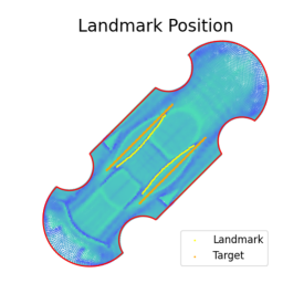
Figure 12: The landmarks and target position, drawing on the car surface parametrization result previously without landmark matching. The yellow dots are the landmarks, while the orange dots are the target positions. The plot is rotated $45^{\circ}$.

The next experiment extends the car surface parametrization to include landmark matching. The landmarks and target positions are illustrated in Figure 12, based on the previous parametrization result. The landmarks chosen are the points on the two upper edges of the two side windows, totally $134$ points, while the target consists of $400$ points sampled from two straight lines $[-0.5,0.5]\times\{-0.25,0.25\}$. The landmark matching is done by treating the two edges of the windows as a single landmark, and the two straight lines as a single target, instead of dividing them into two pairs.

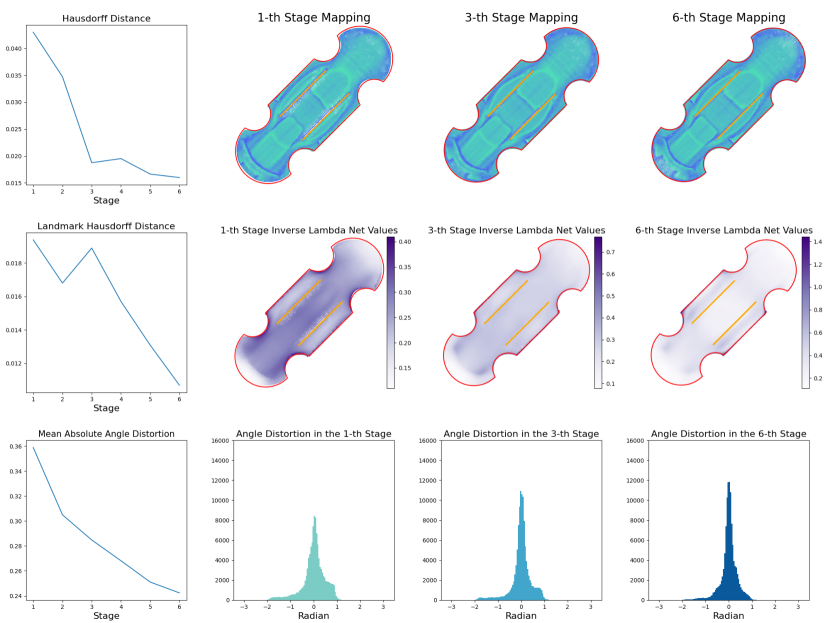
Figure 13: Results for parametrizing a car surface, to a prescribed car shape domain, together with landmark matching. In the first column, line plot for Hausdorff distance for matching parameter domain against stages, line plot for Hausdorff distance for landmark matching against stages, line plot for mean absolute angle distortion (in radian) are plotted from top to bottom. The second to the last columns show the result after the $1^{\text{st}}$, $3^{\text{rd}}$ and $6^{\text{th}}$ stages, including output mappings, $\lambda_{inv}$ networks output values, histogram for angle distortion (in radian) from top to bottom. The yellow dots are the landmarks, while the orange dots are the target positions. The red lines indicate the boundary of the car shape. The mappings and $\lambda_{inv}$ plots are rotated $45^{\circ}$.

The parametrization results with landmark matching are demonstrated in Figure 13. The line plots in the first column show the Hausdorff distance between point cloud mapping with parameter domain, the Hausdorff distance between landmark mapping and target position, and the mean absolute angle distortion against stages. The other three columns show the mappings, $\lambda_{inv}$ and histograms for angle distortion after $1^{\text{st}}$, $3^{\text{rd}}$, $6^{\text{th}}$ stages, as before. The improvement in matching parameter domain and preserving geometry is observed through the decrease in Hausdorff distance with parameter domain and mean absolute angle distortion. The landmark mappings are drawn in yellow, and targets are drawn in orange. However, the yellow points are barely visible, indicating that the landmark mappings and targets are well-aligned. Also, the line plot for landmark Hausdorff distance shows a decreasing trend, indicating an improvement in landmark matching, even though this improvement is not clearly visible in the mapping plots.

8 Applications

In this section, we discuss and introduce some of the applications of our proposed methods, including boundary detection and surface reconstruction.

Boundary information on the point cloud surface is not required in our energy minimizing approaches. In contrast, the boundary of the point cloud surface can be detected using our parametrization. The method is demonstrated on the simply connected human face and car surface. The result mappings of free-boundary parametrization, shown in Figure 7, are used.

In our methods, the free-boundary parametrization minimizes LEG $D_{\sigma}(f,\lambda_{inv},\mathcal{X})$ to obtain the mapping $f(\mathcal{X})$. Delaunay triangulation is then applied on $f(\mathcal{X})$, obtain a triangular mesh structure $(f(\mathcal{X}),\mathcal{T})$. Using the obtained connectivities $\mathcal{T}$, we can form a surface mesh $(\mathcal{X},\mathcal{T})$.

However, the Delaunay triangulation gives the triangulation of the convex hull of $f(\mathcal{X})$, but since the mapping is not always convex, some nonsensical triangular faces may be included. Suppose the all edge lengths of the ground truth surface mesh are shorter than $h>0$. The triangular faces in $(\mathcal{X},\mathcal{T})$ with at least one edge longer than $h$ can be defined as extra faces and removed from $\mathcal{T}$. Boundary detection is then applied to the refined triangular mesh to obtain the boundary of the point cloud.

The result free-boundary mappings of human face and car surface, shown in Figures 7, are used, and the boundary detection results are shown in Figure 14 and 15. By drawing the results on the mappings in 2D plane, the figures show the ground truth boundaries for comparison, the convex hulls of the point cloud mappings, and the predicted boundaries with different choices of threshold $h$, all drawn in red lines. The results demonstrate that the predicted boundaries with an appropriate choice of $h$ successfully recover the ground truth boundaries.

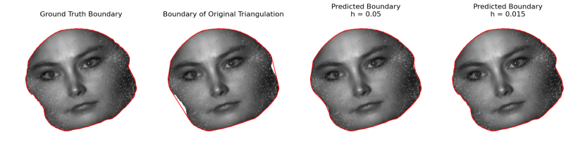
Figure 14: Result of boundary detection on a human face. Left to right: ground truth boundary, convex hull, and two predicted boundaries with threshold $h=0.05,0.015$

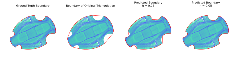
Figure 15: Result of boundary detection on a car surface. Left to right: ground truth boundary, convex hull, and two predicted boundaries with threshold $h=0.25,0.05$

The next application is on surface reconstruction, which recovers a triangular mesh structure from a point cloud. In the previous application on boundary detection, a triangular mesh is generated in the intermediate process as a byproduct. Here, another approach for surface reconstruction is discussed. By parametrizing the point cloud surface to a parameter domain, a 2D triangular mesh in the parameter domain can be created. The inverse mapping of the vertices of the newly created mesh can be obtained via interpolation using the mapping of the point cloud. A reconstructed surface triangular mesh can then be formed using pre-images of the vertices and their connectivity. Comparing to generating triangular mesh directly from the point cloud, this approach provides more robustness to the quality of the point cloud.

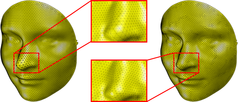
Figure 16: The human face triangular meshes reconstructed from uniform mesh (left) and $\lambda_{inv}-$depended mesh (right). The close-ups to their noses are shown in the red boxes.

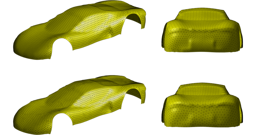
Figure 17: The car triangular meshes reconstructed from uniform mesh (upper) and $\lambda_{inv}-$depended mesh (lower). They are viewed from the side (left) and back (right).

In creating the 2D triangular meshes on the parameter domains, we tried two methods: one was to create a uniform mesh, and the other was to create a mesh with edge lengths are depending on the values of $\lambda_{inv}$ networks. More specifically, for the latter method, the edge lengths were approximately proportional to $1/\sqrt{\lambda_{inv}}$. The idea is that the value represents the scaling of Euclidean distance between the original point cloud and its mapping, thereby creating a triangular mesh with more uniform sizes of triangular faces.

The surface of human face in Figure 8 and car in Figure 11 are reconstructed with the two described methods. The reconstruction results are shown in Figures 16 and 17. Close-ups of the noses, and a back view of the car surfaces are displayed. The size of the triangular faces on the mesh, depending on values of $\lambda_{inv}$, can be observed to be more uniform.

9 Conclusions

In this paper, we have developed a new framework for point cloud surface parametrization. The framework includes formulating the problem as an optimization problem using two novel loss functions, enabling parametrization of surfaces to a parameter domain with connectivity and boundary information. Neural networks are used to model the functions in the optimization problem, and an optimization scheme has also been developed for the purpose.

The two loss functions, Hausdorff Approximation from Node-wise Distances (HAND), for approximating to Hausdorff distance, and Localized Energy for Geometry (LEG), for measuring geometric distortion on point cloud, are presented along with theoretical analysis proving their underlying geometric meaning. HAND provides an differentiable estimation for Hausdorff distance. It can be used for mapping point cloud surfaces, without boundary information, to desired parameter domains, even with complicated shapes or topologies. Also, it can be used for generalized landmark matching, allowing region-wise correspondence and unbalanced number of points in landmarks and targets. On the other hand, LEG estimates a weighted angle distortion on the underlying ground truth triangular mesh structures, without any connectivity information.

The functions $f$ and $\lambda_{inv}$ in the optimization problem are modeled by neural networks. An optimization scheme, which divides the whole optimization process into several stages to improve the parametrization quality, is presented. The idea is simple: the batch size, number of epochs, and some parameters are adjusted after each stage.

The experiments are conducted in various manners, including shape matching, free-boundary parametrization, and fixed-boundary parametrization with and without landmark matching. Despite the random initialization, the matches between point cloud mappings and parameter domains, and between landmark mappings and targets, are accurate. Additionally, the geometry between the mappings and original surfaces is well preserved, suggesting that our methods are robust to initial values.

As the boundary and connectivity information are not required in the proposed methods, boundary detection and surface reconstruction are conducted as applications.

Some potential future directions of our methods include acceleration for processing large datasets of point clouds, extension to closed surfaces and non-planar domains, or high dimensional mapping problems. Further controls on the geometry or matching boundary or landmarks for more specific applications can also be investigated.

References

- [1] P. Achlioptas, O. Diamanti, I. Mitliagkas, and L. Guibas, Learning representations and generative models for 3d point clouds, in International conference on machine learning, PMLR, 2018, pp. 40–49.
- [2] K. Asadi and M. L. Littman, An alternative softmax operator for reinforcement learning, in International Conference on Machine Learning, PMLR, 2017, pp. 243–252.
- [3] J. Bednarik, S. Parashar, E. Gundogdu, M. Salzmann, and P. Fua, Shape reconstruction by learning differentiable surface representations, in Proceedings of the IEEE/CVF Conference on Computer Vision and Pattern Recognition, 2020, pp. 4716–4725.
- [4] M. Belkin and P. Niyogi, Towards a theoretical foundation for laplacian-based manifold methods, Journal of Computer and System Sciences, 74 (2008), pp. 1289–1308.
- [5] M. Belkin, J. Sun, and Y. Wang, Constructing laplace operator from point clouds in , in Proceedings of the twentieth annual ACM-SIAM symposium on Discrete algorithms, SIAM, 2009, pp. 1031–1040.
- [6] M. M. Bronstein, J. Bruna, Y. LeCun, A. Szlam, and P. Vandergheynst, Geometric deep learning: going beyond euclidean data, IEEE Signal Processing Magazine, 34 (2017), pp. 18–42.
- [7] Q. Chen, Z. Li, and L. M. Lui, A deep learning framework for diffeomorphic mapping problems via quasi-conformal geometry applied to imaging, SIAM Journal on Imaging Sciences, 17 (2024), pp. 501–539.
- [8] E. Chien, Z. Levi, and O. Weber, Bounded distortion parametrization in the space of metrics, ACM Transactions on Graphics (TOG), 35 (2016), pp. 1–16.
- [9] G. P. Choi, Efficient conformal parameterization of multiply-connected surfaces using quasi-conformal theory, Journal of Scientific Computing, 87 (2021), p. 70.
- [10] G. P. Choi, B. Chiu, and C. H. Rycroft, Area-preserving mapping of 3d carotid ultrasound images using density-equalizing reference map, IEEE Transactions on Biomedical Engineering, 67 (2020), pp. 2507–2517.
- [11] G. P. Choi, Y. Leung-Liu, X. Gu, and L. M. Lui, Parallelizable global conformal parameterization of simply-connected surfaces via partial welding, SIAM Journal on Imaging Sciences, 13 (2020), pp. 1049–1083.
- [12] G. P. Choi and L. M. Lui, Recent developments of surface parameterization methods using quasi-conformal geometry, Handbook of Mathematical Models and Algorithms in Computer Vision and Imaging: Mathematical Imaging and Vision, (2022), pp. 1–41.
- [13] G. P. Choi and C. H. Rycroft, Density-equalizing maps for simply connected open surfaces, SIAM Journal on Imaging Sciences, 11 (2018), pp. 1134–1178.
- [14] G. P.-T. Choi, K. T. Ho, and L. M. Lui, Spherical conformal parameterization of genus-0 point clouds for meshing, SIAM Journal on Imaging Sciences, 9 (2016), pp. 1582–1618.
- [15] G. P. T. Choi, Y. Liu, and L. M. Lui, Free-boundary conformal parameterization of point clouds, Journal of Scientific Computing, 90 (2021), p. 14, https://doi.org/10.1007/s10915-021-01641-6, https://doi.org/10.1007/s10915-021-01641-6.
- [16] P. T. Choi, K. C. Lam, and L. M. Lui, Flash: Fast landmark aligned spherical harmonic parameterization for genus-0 closed brain surfaces, SIAM Journal on Imaging Sciences, 8 (2015), pp. 67–94.
- [17] P. T. Choi and L. M. Lui, Fast disk conformal parameterization of simply-connected open surfaces, Journal of Scientific Computing, 65 (2015), pp. 1065–1090, https://doi.org/10.1007/s10915-015-9998-2, https://doi.org/10.1007/s10915-015-9998-2.
- [18] T. Deprelle, T. Groueix, M. Fisher, V. Kim, B. Russell, and M. Aubry, Learning elementary structures for 3d shape generation and matching, Advances in Neural Information Processing Systems, 32 (2019).
- [19] M. Desbrun, M. Meyer, and P. Alliez, Intrinsic parameterizations of surface meshes, in Computer graphics forum, vol. 21, Wiley Online Library, 2002, pp. 209–218.
- [20] M. T. Gastner and M. E. Newman, Diffusion-based method for producing density-equalizing maps, Proceedings of the National Academy of Sciences, 101 (2004), pp. 7499–7504.
- [21] I. Goodfellow, Y. Bengio, and A. Courville, Deep Learning, MIT Press, 2016. http://www.deeplearningbook.org.
- [22] T. Groueix, M. Fisher, V. G. Kim, B. C. Russell, and M. Aubry, 3d-coded: 3d correspondences by deep deformation, in Proceedings of the european conference on computer vision (ECCV), 2018, pp. 230–246.
- [23] T. Groueix, M. Fisher, V. G. Kim, B. C. Russell, and M. Aubry, A papier-mâché approach to learning 3d surface generation, in Proceedings of the IEEE conference on computer vision and pattern recognition, 2018, pp. 216–224.
- [24] X. Gu, Y. Wang, T. F. Chan, P. M. Thompson, and S.-T. Yau, Genus zero surface conformal mapping and its application to brain surface mapping, IEEE transactions on medical imaging, 23 (2004), pp. 949–958.
- [25] X. Gu and S.-T. Yau, Global conformal surface parameterization, in Proceedings of the 2003 Eurographics/ACM SIGGRAPH symposium on Geometry processing, 2003, pp. 127–137.
- [26] X. Gu and S.-T. Yau, Computational Conformal Geometry, vol. 3 of Advanced Lectures in Mathematics, International Press and Higher Education Press, 2007.
- [27] Y. Guo, Q. Chen, G. P. Choi, and L. M. Lui, Automatic landmark detection and registration of brain cortical surfaces via quasi-conformal geometry and convolutional neural networks, Computers in Biology and Medicine, 163 (2023), p. 107185.
- [28] M. Jin, J. Kim, F. Luo, and X. Gu, Discrete surface ricci flow, IEEE Transactions on Visualization and Computer Graphics, 14 (2008), pp. 1030–1043.
- [29] D. Karimi and S. E. Salcudean, Reducing the hausdorff distance in medical image segmentation with convolutional neural networks, IEEE Transactions on medical imaging, 39 (2019), pp. 499–513.
- [30] L. Kharevych, B. Springborn, and P. Schröder, Discrete conformal mappings via circle patterns, ACM Transactions on Graphics (TOG), 25 (2006), pp. 412–438.
- [31] P. Koebe, Über die konforme abbildung mehrfach zusammenhängender bereiche., Jahresbericht der Deutschen Mathematiker-Vereinigung, 19 (1910), pp. 339–348, http://eudml.org/doc/145249.
- [32] K. C. Lam and L. M. Lui, Landmark and intensity based registration with large deformations via quasi-conformal maps, SIAM Journal on Imaging Sciences, 7 (2014), pp. 2364–2392.
- [33] C. Lange and K. Polthier, Anisotropic smoothing of point sets, Computer Aided Geometric Design, 22 (2005), pp. 680–692.
- [34] B. Lévy, S. Petitjean, N. Ray, and J. Maillot, Least squares conformal maps for automatic texture atlas generation, in Seminal Graphics Papers: Pushing the Boundaries, Volume 2, 2023, pp. 193–202.
- [35] J. Liang, R. Lai, T. W. Wong, and H. Zhao, Geometric understanding of point clouds using laplace-beltrami operator, in 2012 IEEE conference on computer vision and pattern recognition, IEEE, 2012, pp. 214–221.
- [36] J. Liang and H. Zhao, Solving partial differential equations on point clouds, SIAM Journal on Scientific Computing, 35 (2013), pp. A1461–A1486.
- [37] L. M. Lui, K. C. Lam, T. W. Wong, and X. Gu, Texture map and video compression using beltrami representation, SIAM Journal on Imaging Sciences, 6 (2013), pp. 1880–1902.
- [38] L. M. Lui, T. W. Wong, P. Thompson, T. Chan, X. Gu, and S.-T. Yau, Shape-based diffeomorphic registration on hippocampal surfaces using beltrami holomorphic flow, in Medical Image Computing and Computer-Assisted Intervention–MICCAI 2010: 13th International Conference, Beijing, China, September 20-24, 2010, Proceedings, Part II 13, Springer, 2010, pp. 323–330.
- [39] L. M. Lui, T. W. Wong, W. Zeng, X. Gu, P. M. Thompson, T. F. Chan, and S.-T. Yau, Optimization of surface registrations using beltrami holomorphic flow, Journal of Scientific Computing, 50 (2012), pp. 557–585, https://doi.org/10.1007/s10915-011-9506-2, https://doi.org/10.1007/s10915-011-9506-2.
- [40] F. Luo, Combinatorial yamabe flow on surfaces, Communications in Contemporary Mathematics, 6 (2004), pp. 765–780.
- [41] Z. Lyu, G. P. Choi, and L. M. Lui, Bijective density-equalizing quasiconformal map for multiply connected open surfaces, SIAM Journal on Imaging Sciences, 17 (2024), pp. 706–755.
- [42] Z. Lyu, L. M. Lui, and G. Choi, Spherical density-equalizing map for genus-0 closed surfaces, arXiv preprint arXiv:2401.11795, (2024).
- [43] Q. Meng, B. Li, H. Holstein, and Y. Liu, Parameterization of point-cloud freeform surfaces using adaptive sequential learning rbfnetworks, Pattern Recognition, 46 (2013), pp. 2361–2375.
- [44] T. Meng and L. M. Lui, Pcbc: Quasiconformality of point cloud mappings, Journal of Scientific Computing, 77 (2018), pp. 597–633.
- [45] T. W. Meng, G. P.-T. Choi, and L. M. Lui, Tempo: feature-endowed teichmuller extremal mappings of point clouds, SIAM Journal on Imaging Sciences, 9 (2016), pp. 1922–1962.
- [46] L. Mescheder, M. Oechsle, M. Niemeyer, S. Nowozin, and A. Geiger, Occupancy networks: Learning 3d reconstruction in function space, in Proceedings of the IEEE/CVF conference on computer vision and pattern recognition, 2019, pp. 4460–4470.
- [47] L. Morreale, N. Aigerman, P. Guerrero, V. G. Kim, and N. J. Mitra, Neural convolutional surfaces, in Proceedings of the IEEE/CVF Conference on Computer Vision and Pattern Recognition, 2022, pp. 19333–19342.
- [48] L. Morreale, N. Aigerman, V. G. Kim, and N. J. Mitra, Neural surface maps, in Proceedings of the IEEE/CVF Conference on Computer Vision and Pattern Recognition, 2021, pp. 4639–4648.
- [49] P. Mullen, Y. Tong, P. Alliez, and M. Desbrun, Spectral conformal parameterization, in Computer Graphics Forum, vol. 27, Wiley Online Library, 2008, pp. 1487–1494.
- [50] A. Paszke, S. Gross, F. Massa, A. Lerer, J. Bradbury, G. Chanan, T. Killeen, Z. Lin, N. Gimelshein, L. Antiga, et al., Pytorch: An imperative style, high-performance deep learning library, Advances in neural information processing systems, 32 (2019).
- [51] C. R. Qi, H. Su, K. Mo, and L. J. Guibas, Pointnet: Deep learning on point sets for 3d classification and segmentation, in Proceedings of the IEEE conference on computer vision and pattern recognition, 2017, pp. 652–660.
- [52] C. R. Qi, L. Yi, H. Su, and L. J. Guibas, Pointnet++: Deep hierarchical feature learning on point sets in a metric space, Advances in neural information processing systems, 30 (2017).
- [53] D. Qiu, K.-C. Lam, and L.-M. Lui, Computing quasi-conformal folds, SIAM Journal on Imaging Sciences, 12 (2019), pp. 1392–1424.
- [54] R. Schoen and S. Yau, Lectures on Differential Geometry, Conference Proceedings and Lecture Note, International Press, 1994, https://books.google.com.hk/books?id=d4VtQgAACAAJ.
- [55] G. Sharma, D. Liu, S. Maji, E. Kalogerakis, S. Chaudhuri, and R. Měch, Parsenet: A parametric surface fitting network for 3d point clouds, in Computer Vision–ECCV 2020: 16th European Conference, Glasgow, UK, August 23–28, 2020, Proceedings, Part VII 16, Springer, 2020, pp. 261–276.
- [56] K. Su, L. Cui, K. Qian, N. Lei, J. Zhang, M. Zhang, and X. D. Gu, Area-preserving mesh parameterization for poly-annulus surfaces based on optimal mass transportation, Computer Aided Geometric Design, 46 (2016), pp. 76–91.
- [57] G. Tewari, C. Gotsman, and S. J. Gortler, Meshing genus-1 point clouds using discrete one-forms, Computers & Graphics, 30 (2006), pp. 917–926.
- [58] T. Tieleman and G. Hinton, Lecture 6.5-rmsprop: Divide the gradient by a running average of its recent magnitude, COURSERA: Neural networks for machine learning, 4 (2012), p. 26.
- [59] Y. Wang, X. Gu, K. M. Hayashi, T. F. Chan, P. M. Thompson, and S.-T. Yau, Brain surface parameterization using riemann surface structure, in Medical Image Computing and Computer-Assisted Intervention–MICCAI 2005: 8th International Conference, Palm Springs, CA, USA, October 26-29, 2005, Proceedings, Part II 8, Springer, 2005, pp. 657–665.
- [60] Y. Wang, Y. Sun, Z. Liu, S. E. Sarma, M. M. Bronstein, and J. M. Solomon, Dynamic graph cnn for learning on point clouds, ACM Transactions on Graphics (tog), 38 (2019), pp. 1–12.
- [61] O. Weber, A. Myles, and D. Zorin, Computing extremal quasiconformal maps, in Computer Graphics Forum, vol. 31, Wiley Online Library, 2012, pp. 1679–1689.
- [62] T. Wu and S.-T. Yau, Computing harmonic maps and conformal maps on point clouds, arXiv preprint arXiv:2009.09383, (2020).
- [63] Y. Yang, C. Feng, Y. Shen, and D. Tian, Foldingnet: Point cloud auto-encoder via deep grid deformation, in Proceedings of the IEEE conference on computer vision and pattern recognition, 2018, pp. 206–215.
- [64] Y.-L. Yang, R. Guo, F. Luo, S.-M. Hu, and X. Gu, Generalized discrete ricci flow, in Computer graphics forum, vol. 28, Wiley Online Library, 2009, pp. 2005–2014.
- [65] M.-H. Yueh, Theoretical foundation of the stretch energy minimization for area-preserving simplicial mappings, SIAM Journal on Imaging Sciences, 16 (2023), pp. 1142–1176.
- [66] M.-H. Yueh, W.-W. Lin, C.-T. Wu, and S.-T. Yau, An efficient energy minimization for conformal parameterizations, Journal of Scientific Computing, 73 (2017), pp. 203–227.
- [67] M.-H. Yueh, W.-W. Lin, C.-T. Wu, and S.-T. Yau, A novel stretch energy minimization algorithm for equiareal parameterizations, Journal of Scientific Computing, 78 (2019), pp. 1353–1386.
- [68] W. Zeng, L. M. Lui, F. Luo, T. F.-C. Chan, S.-T. Yau, and D. X. Gu, Computing quasiconformal maps using an auxiliary metric and discrete curvature flow, Numerische Mathematik, 121 (2012), pp. 671–703, https://doi.org/10.1007/s00211-012-0446-z, https://doi.org/10.1007/s00211-012-0446-z.
- [69] W. Zeng, X. Yin, M. Zhang, F. Luo, and X. Gu, Generalized koebe’s method for conformal mapping multiply connected domains, in 2009 SIAM/ACM Joint Conference on Geometric and Physical Modeling, 2009, pp. 89–100.
- [70] D. Zhang, G. P. Choi, J. Zhang, and L. M. Lui, A unifying framework for n-dimensional quasi-conformal mappings, SIAM Journal on Imaging Sciences, 15 (2022), pp. 960–988.
- [71] L. Zhang, L. Liu, C. Gotsman, and H. Huang, Mesh reconstruction by meshless denoising and parameterization, Computers & Graphics, 34 (2010), pp. 198–208.
- [72] X. Zhao, Z. Su, X. D. Gu, A. Kaufman, J. Sun, J. Gao, and F. Luo, Area-preservation mapping using optimal mass transport, IEEE transactions on visualization and computer graphics, 19 (2013), pp. 2838–2847.
- [73] Z. Zhu, G. P. Choi, and L. M. Lui, Parallelizable global quasi-conformal parameterization of multiply connected surfaces via partial welding, SIAM Journal on Imaging Sciences, 15 (2022), pp. 1765–1807.
- [74] M. Zwicker and C. Gotsman, Meshing point clouds using spherical parameterization., in PBG, Citeseer, 2004, pp. 173–180.