Discrete Layered Entropy, Conditional Compression and a Tighter Strong Functional Representation Lemma
Abstract
We study a quantity called discrete layered entropy, which approximates the Shannon entropy within a logarithmic gap. Compared to the Shannon entropy, the discrete layered entropy is piecewise linear, approximates the expected length of the optimal one-to-one non-prefix-free encoding, and satisfies an elegant conditioning property. These properties make it useful for approximating the Shannon entropy in linear programming, studying the optimal length of conditional encoding, and bounding the entropy of monotonic mixture distributions. In particular, it can give a bound for the strong functional representation lemma that improves upon the best bound (as long as the mutual information is at least 2).
I Introduction
In this paper, we study a quantity which we call discrete layered entropy
where is a probability mass function, is the -th entry of when sorted in descending order. This is a discrete analogue of the (continuous) layered entropy studied in [1, 2]. Compared to the Shannon entropy , has the following properties:
-
•
transforms nicer for joint random variable (e.g., for independent ), whereas transforms nicer for conditioning ().
- •
-
•
is close to within a logarithmic gap.
We present several applications of . First, it can be used to show a tighter strong functional representation lemma: for every , there exists independent of with and , which improves upon previous results [6, 7, 8] for . We will also show another bound that improves upon [8] for . Second, it is a piecewise linear approximation of useful for linear programming. Third, it is useful for conditional encoding tasks, to be described as follows.
Suppose the encoder wants to encode , given a side information that is also known to the decoder (i.e., the encoder encodes conditionally given ). One method is to have the encoder find the ranking of among for all (i.e., has the -th largest ), and sends to the decoder. This can be shown to be smallest possible compression, in the sense that it minimizes (which is approximately the compression size using a prefix-free code)111If we are allowed to encode conditional on using a conditional prefix-free code, then the compression size would be . Nevertheless, if we require synchronization even when the decoder does not know , then we must use an unconditional prefix-free code, which has a length . Refer to Section IV-B for discussions. subject to the recoverability requirement . Hence, this can be regarded as the “conditional compression” of given , which contains the information in that is not in , and hence we use the notation to highlight the analogy to set difference.
It is perhaps unsatisfying that the entropy of the conditional compression is generally not the conditional entropy (we only have ). The conditional entropy does not actually correspond to the entropy of any random variable—it cannot be interpreted as the entropy applied to a “conditional random variable ”. This is in stark contrast to the joint entropy , which is indeed applied to the joint random variable .
We show that discrete layered entropy satisfies
| (1) |
where is defined in a similar manner as . This fact is not only aesthetically pleasing (we can indeed treat “” as a random variable given by ), but also has several implications. First, this allows us to approximate the optimal expected encoding length of the aforementioned conditional encoding task by . Second, it makes a useful tool for bounding the entropy of a mixture of distributions with monotonic probability mass functions, since (1) is equivalent to saying that is a linear function of the probability mass function when we restrict to a nondecreasing function. We will utilize this to prove a tighter bound for the strong functional representation lemma [6] in Section VI.
Moreover, we show that (1) is the defining property of , in the sense that the discrete layered entropy is the only function satisfying (1) and for . Also, is the largest function satisfying (1) and , and hence is the “best underestimate” of that satisfies (1). We show that is close to , in the sense that
| (2) |
This allows us to convert between and depending on whether we need the properties of or in the proof, incurring only a logarithmic gap for each conversion. This makes a powerful tool even if we only want our final result to be in terms of Shannon entropy. For example, for the conditional encoding task, we can approximate the optimal encoding length using (1) and (2) via .
Related Works on Differences between Information
Apart from the “” (which minimizes subject to ) studied in this paper, there are several notions of differences between the information in and the information in studied in the literature.
Strong functional representation lemma [6] seeks to minimize subject to and . These constraints are analogous to set differences between sets , which satisfies and . Note that can be much larger than . To review various bounds on , the result in [9] implies that can be achieved, where . [10] improved the bound to ; [6] improved it to ; [7] improved it to ; and [8] improved it to . See [11] for a review. In Section VI, we show a new bound , which improves upon [7] for every , and improves upon [8] for . These improved bounds show the usefulness of as a technical tool.
Notions that can be interpreted as difference have been studied systematically in [12]. It was argued that apart from the strong functional representation lemma, the Körner graph entropy [13] and the maximum rate for perfect privacy [14] can be treated as the difference between and . The minimum entropy coupling [15, 16, 17, 18] has also been related to the difference between information.
Notations
Throughout this paper, all random variables are assumed to be discrete (with finite or countable support) unless otherwise stated. Entropy is in bits, and is to the base . Write , (let ). For a random variable , write for the set it lies in, and for its probability mass function (pmf). For random variables , we say that they are (informationally) equivalent, denoted as , if . Denote the constant random variable as (so means that is a constant). Write . The min-entropy is defined as .
For a pmf over , write for a pmf over , where is the -th entry of when sorted in descending order ( if ). Given pmfs , we say that majorizes , written as , if for every [22]. A function mapping pmfs to real numbers is Schur concave if implies . For example, Shannon entropy is Schur concave.
II Discrete Layered Entropy
We now define the central quantity of this paper.
Definition 1 (Discrete layered entropy).
The discrete layered entropy of a probability mass function is defined as
| (3) |
Recall that is the -th entry of when sorted in descending order, and we assume . We write . The conditional discrete layered entropy of a random variable given another random variable is
We use the name “discrete layered entropy” since is the discrete analogue of the (continuous) layered entropy studied in [1, 2], which is shown in (5).222The notation “” is chosen for two reasons—both “layered” and “lambda” starts with “la”, and the shape “” mimics the shape of the function (a piecewise-linear concave function) when is binary. We give several alternative definitions for . The proof is given in Appendix -A.
Proposition 2 (Alternative definitions).
We have
-
1.
(Integral form)
(4) -
2.
(Layered form)
(5) -
3.
(Concave envelope of min-entropy)
(6) where is the conditional min-entropy. In other words, is the upper concave envelope of .333This means where the minimum is over concave functions satisfying for all .
-
4.
(Concave envelope of log cardinality)
(7) where the maximum is over such that is a uniform distribution for every , i.e., for every such that .444This is the discrete analogue of the alternative definition of continuous layered entropy in [2]. Equivalently, , where the minimum is over all concave functions satisfying when is uniformly distributed.
-
5.
(Linear programming form)
(8) where the maximum is over joint probability mass functions over with an -marginal that coincides with , and satisfying that for all , where is the -marginal of . This means can be formulated as a maximization in a linear program when is finite.
Another alternative definition of will be given in Theorem 8. We then show some basic properties of . The proof is given in Appendix -B.
Proposition 3 (Basic properties).
We have, for every random variables , ,
-
1.
. For each inequality, equality holds if and only if is uniformly distributed.
-
2.
(Concavity) is a concave function over probability mass functions . Equivalently, .
-
3.
(Schur concavity) is Schur concave, and hence if .
-
4.
(Monotone linearity) is a linear function over the convex space of nondecreasing probability mass functions . Equivalently, if , and for every fixed , is a nondecreasing function, then . (Overall, is a piecewise linear function over the space of not-necessarily-nondecreasing probability mass functions.)
-
5.
(Superadditivity) If are independent, then
Equality holds if and only if at least one of is uniformly distributed.
-
6.
(Bounded increase) For any ,
Equality holds if and only if is uniformly distributed and is independent of .
One of the most useful property of is that is close to within a logarithmic gap. The proof is in Appendix -C.
Proposition 4 ().
For every discrete ,
| (9) |
for every . In particular, taking gives a bound good for large :
Taking gives a bound good for small :
Note that (where ) is minimized at . This gives the best bound for (9), but is a little unwieldy.
Proposition 4 shows that is a good approximate of , and can be used in place of when the properties of are more desirable. For example, consider the entropy maximization problem where is a convex polytope of probability vectors. This cannot be solved via linear programming since is not piecewise linear/affine. Moreover, has undefined gradient when there is a zero entry in , making it difficult to solve the problem via gradient-based methods. On the other hand, the layered entropy maximization problem can be solved via linear programming by (8). By Proposition 4, the optimal values of the two problems are close within a logarithmic gap, making a good substitute for . In the following sections, we will see more theoretical properties of that are not satisfied by .
III Relation to One-to-one Non-prefix-free Codes
A one-to-one (non-prefix-free) code is an injective function which is not subject to the prefix-free requirement [3, 4, 5]. The optimal expected length of a one-to-one encoding of is [3, 4]
We show that is approximated by within bits. This is in contrast to which approximates the expected length of prefix-free codes. The proof is in Appendix -D.
Proposition 5.
We have
Using Propositions 4 and 5, we can show that the optimal expected length of one-to-one codes is at least , giving a similar (and slightly weaker) bound compared to [3, 4]. By [5], when is an i.i.d. sequence following , as ,
One may raise the question—why should we study instead of which is exactly the optimal length? Indeed, also satisfies some properties of , such as concavity, monotone linearity and the conditional property to be discussed in Proposition 9. One reason for preferring is that approximates better than . We have , and whenever is uniform, whereas the expression of for uniform is complicated. This not only allows to satisfy more elegant theoretical properties compared to (Theorems 8, 11, 12, and some properties in Proposition 3), but also makes a more useful tool for approximation tasks (e.g., Theorem 16).
IV Conditional Compression and “Three Conditional Entropies”
IV-A Conditional Compression
Given random variables , we are interested in finding “the information in that is not in ”. Intuitively, it is the smallest such that can be recovered using . It is formally defined below.
Definition 6 (Conditional compression).
We say that a random variable is a conditional compression of given if is a minimizer of subject to the constraint .555Equivalently, by Proposition 7, we can consider that gives the maximum distribution with respect to majorization, subject to . The canonical conditional compression of given , written as , is the conditional compression that minimizes among all conditional compressions.
The distribution of a conditional compression can be found.
Proposition 7.
The probability mass function of any conditional compression of given must satisfy
for , where is the -th entry of when sorted in descending order.
Proof:
We can find a conditional compression in the following way. For each , we sort the values of in descending order to obtain , where are distinct values. Take to be the value that satisfies , i.e., is the ranking of among ( is the -th largest among for ). We then have .
To show that this is indeed a conditional compression (it minimizes ), consider any other satisfying . Hence, for every , i.e., . This implies
and , and hence . Equality holds if and only if , i.e., has the same distribution as up to relabeling. Therefore, any conditional compression has the same distribution up to relabeling. ∎
The reason for the notation is that the conditional compression shares a number of properties with set difference. Firstly, (i.e., is a constant) if , corresponding to the fact that for sets if . Secondly, if , analogous to the fact that if . This property is the reason of the tie-breaking rule (minimizing in case of a tie of minimizing ) in the definition of .666Although there may be multiple conditional compressions in case there are ties among , we are usually only interested in the marginal distribution so it does not matter which one we consider (they all have the same distribution). Nevertheless, in order to justify the notation , we select a “canonical” conditional compression in Definition 6 to be the one that minimizes , to ensure that if .
The converse of the first property holds ( if and only if ), but the converse of the second property is false, i.e., does not imply . In fact, is the maximum violation, i.e., is the largest possible subject to . This gives a simple alternative definition of given in Theorem 8. By Proposition 4, if , then , so the converse does approximately hold. The proof of Theorem 8 is in Appendix -E. In Section IV-B, we will discuss the operational meaning of this definition.
Theorem 8 (Alternative definition of ).
We have
Also, if , then .
An elegant property of is that coincides with . Therefore, is indeed the discrete layered entropy of “the random variable ” which is formally given as .
Proposition 9 (Conditioning property).
Equivalently,
| (10) |
We will see in Section IV-C that the conditioning property is actually the defining property of the discrete layered entropy, in the sense that if the function satisfies the conditioning property and if is uniformly distributed, then must be the discrete layered entropy.
We now have three different notions of “conditional entropy”, namely , and . Although Shannon entropy does not satisfy the conditioning property, i.e., is generally not equal to , we can show that via the discrete layered entropy. By Propositions 3 and 4,
| (11) |
Therefore, the three “conditional entropies” are close within a logarithmic gap. We highlight the following theorem that follows directly from (11).
Theorem 10.
For every ,
Theorem 10 can also be stated as: for every , there exists such that , and for every , . This is an example of a nonlinear existential information inequality [23, 24, 25]. It is perhaps interesting that such a simple (and novel, to the best of the author’s knowledge) fact about Shannon entropy can be proved via the properties of discrete layered entropy . It shows the usefulness of as a tool for proving results about Shannon entropy.
Also, unlike set difference where and are disjoint, we do not have . Nevertheless, Theorem 10 implies that this property approximately holds, in the sense that is small.777Compare to the strong functional representation lemma (SFRL) [6, 8]: for every , there exists such that and . SFRL guarantees , whereas we only have . Nevertheless, SFRL does not guarantee (it only has ; the construction in [6] can have extremely large ), whereas we have .
IV-B Conditional Variable-Length Encoding
Consider a one-shot variable-length encoding setting, where there is a source symbol that is correlated with a side information . The encoder observes , and sends a variable-length description to the decoder. The decoder observes , and has to recover losslessly, i.e., . The goal is to make the expected length as small as possible.
If there is no prefix-free requirement on , the task is straightforward—given that , the encoder encodes into using the best non-prefix-free one-to-one code designed for the distribution . Let be the smallest possible in this case. By Proposition 5, . As usual for a non-prefix-free codes, the decoder cannot synchronize with the encoder, i.e., the decoder does not know where ends, unless external help is available (e.g., when is already given by the metadata of the communication protocol).
For the sake of synchronization, given that , this task is conventionally performed by encoding conditional on into , using a prefix-free code designed for the distribution . This gives a “conditionally prefix-free code”, i.e., , where is a prefix-free codebook for every . Let be the smallest possible in this case. Using Huffman coding [26], .
A shortcoming of this approach is that this “conditional prefix-free code” is not a prefix-free code to a party that does not know . This party only knows which may not be a prefix-free codebook. For example, consider , , , . The optimal conditional prefix-free code would be , , , , , which is not prefix-free. This shortcoming can be significant if the decoder does not always know . Without knowing , the decoder not only cannot decode , but also cannot know where the bit sequence ends, and becomes desynchronized with the encoder.
For example, consider a video streaming application where the encoder sends the frames of a video to the decoder. Since consecutive frames are correlated, it is reasonable for the encoder to encode each frame conditional on the previous frame to reduce the encoding size. However, if there is a packet loss, the decoder will be unable to decode all subsequent frames that are encoded conditionally on the previous frames. Therefore, the encoder would occasionally encode some frames (the keyframes) by themselves without conditioning on the previous frames, so the decoder can decode these keyframes even if the previous frames are lost.
Now, consider the scenario where there is a packet loss and the decoder cannot decode the current frame. A new packet arrives which contains some conditionally-encoded frames, with one keyframe in the middle of the packet. If a conditional prefix-free code is used to encode the conditionally-encoded frames, then the decoder will become desynchronized and fail to decode the keyframe. In comparison, if an unconditional prefix-free code is used (i.e., lies in a prefix-free codebook that does not depend on ), then the decoder will be unable to decode the conditionally-encoded frames, but still be able to keep synchronous when it scans through the packet, and hence can decode the keyframe.
Hence, it is of interest to study the setting where is in an unconditionally prefix-free codebook, where we let be the smallest possible . Using Huffman coding [26], is within bit from . We summarize the optimal expected lengths in the three settings:
-
•
For non-prefix-free one-to-one, :
(12) -
•
For conditionally prefix-free, :
(13) -
•
For unconditionally prefix-free, :
(14)
The three “conditional entropies” are close within a logarithmic gap, as shown in (11).
To study the difference between conditionally (13) and unconditionally (14) prefix-free encoding, it is of interest to study the region of possible values of the pair . Given , define
An inner bound of is given by the diagonal line, that is, for every .888To show this, consider a distribution that majorizes [22] with . We can construct random variables such that , is independent of , and . This gives . Since contains the same entries (possibly reordered) as , is a conditional compression of given , and hence . Theorem 10 gives an outer bound of , showing that cannot be too far from the diagonal line.
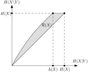
An interesting extreme point of is the minimum of subject to the contraint that is maximized (). The that attains this minimum is the most “conditionally useful” (i.e., giving the shortest conditionally prefix-free encoding length ) among “unconditionally useless” side information (i.e., the unconditionally prefix-free encoding length is the same as if is absent). By Theorem 8, this minimum is given by . Hence, we have another operational meaning of : “if we are to design a side information that provides no benefit to a party that encodes using an unconditionally prefix-free code, how useful can it be to a party that uses a conditionally prefix-free code?”
IV-C Characterizations of via the Conditioning Property
Proposition 8 gives a definition of using only Shannon entropy. In this subsection, we study some more axiomatic definitions of via the conditioning property (Proposition 9). We first show that any function satisfying the conditioning property and for uniform must be the discrete layered entropy. The proof is given in Appendix -F.
Theorem 11.
If is a function mapping discrete distributions to nonnegative real numbers that satisfies the conditioning property (i.e., ), whenever is uniformly distributed over , and whenever (i.e., is invariant under relabeling), then .
Compare this with the axiomatic characterization of Shannon entropy in [27]: if satisfy the subadditivity property (), additivity property ( if ), continuity with respect to the probability mass function, if , and whenever , then is the Shannon entropy . We can see that additivity, subadditivity and continuity are the defining properties of Shannon entropy, whereas conditioning is the defining property of discrete layered entropy.
We then study another characterization of . Recall that does not satisfy the conditioning property. Nevertheless, we can ask what is the best under-approximation of that satisfy the conditioning property. The answer is given by . The proof is in Appendix -G.
Theorem 12.
If is a function mapping discrete distributions to nonnegative real numbers that satisfies the conditioning property, for every ,999Actually, we only need whenever is uniform. and whenever , then for every . Equivalently, admits the following characterization:
where the maximum is over functions that satisfies the conditioning property, for every , and whenever .
V Discrete Rényi Layered Entropy
Rényi entropy [28] is a generalization of Shannon entropy, defined as (where is the order)
Also, define for , which gives , , and . In this section, we generalize the discrete layered entropy to the discrete Rényi layered entropy in an analogous manner.
Definition 13 (Discrete Rényi layered entropy).
Given , the discrete Rényi layered entropy of order of a probability mass function is defined as
| (15) |
where is the -th entry of when sorted in descending order. Also, define for , which can be evaluated as , , and .
We present some properties of . The proof is in Appendix -H.
Proposition 14.
We have the following for :
-
•
is non-increasing in , and .
-
•
When is uniformly distributed, .
-
•
If , then
In particular, .
Remark 15.
Given (6), another way to modify Rényi entropy to incorporate is to study the concave envelope of the Rényi entropy
where . Since is already concave for , we have for . We also have . Therefore, we can use to interpolate between and . The properties of are left for future studies.
VI Strong Functional Representation Lemma
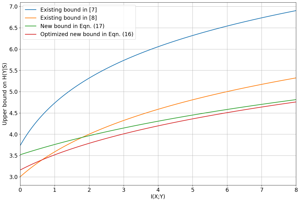
Using the properties of , we can give a tighter bound for the strong functional representation lemma which improves upon [6, 7, 8] for . If we optimize over , then this improves upon [8] for . The proof is in Appendix -I.
Theorem 16.
For every (not necessarily discrete) random variables , there exists a (not necessarily discrete) random variable such that is independent of , , and
Hence, for every ,
| (16) |
In particular, substituting gives
| (17) |
Refer to Figure 3 for a comparison between Theorem 16 and previous bounds. It includes the plot of the bound (writing ) in [7]; in [8]; our new bound (17); and our new bound (16) when optimized over (the optimal is where ).
VII Acknowledgement
This work was partially supported by two grants from the Research Grants Council of the Hong Kong Special Administrative Region, China [Project No.s: CUHK 24205621 (ECS), CUHK 14209823 (GRF)].
-A Proof of Proposition 2
We then prove
| (18) |
where the minimum is over all concave functions satisfying when is uniformly distributed. Assume and is in descending order without loss of generality. Note that
is a convex combination of uniform distributions . Hence, for every concave satisfying that , we have
To show that there exists satisfying whenever is uniform and for this fixed , we take
to be a linear function. We have . For any uniform , we have
Hence, .
For (7), if is conditionally uniform given , then by concavity (the concavity of follows from (18)). To show that is achievable, consider a random variable distributed as (if we want to be discrete, we can discretize by dividing at the points ). Note that is the uniform distribution over , and hence is achievable by (5).
-B Proof of Proposition 3
We have already proved in Appendix -A. follows from (7). From direct evaluation, for uniform . To show implies that is uniform, by (7), if , then there exists such that is conditionally uniform given and , implying that , and is uniform.
The concavity of follows from (18). Schur concavity follows from concavity and the fact that is invariant under labelling of . Monotone linearity follows directly from the definition of .
For superadditivity, let and where attain the maximum in (7), and . Since is uniform conditional on , and is uniform conditional on , is uniform conditional on , and hence by (7). We then show the equality case. If , then . Let , . We have . For , if neither of or contains the other, then
since has a different ordering as , and hence does not achieve the maximum of subject to that is conditionally uniform given . Therefore, for every , one of or contains the other. This is impossible if there are two possible sets for and two possible sets for (in this case, we can take and ). Hence, there is only one possible set for (implying is uniform), or there is only one possible set for (implying is uniform).
For bounded increase, assume , , is in descending order, and is in decreasing order with respect to for every fixed without loss of generality. Let . Then has the same information as . Letting , we have
where (a) and (b) are by rearrangement inequality where is the -th largest entry of . If , then equality in (a) and (b) holds, so we must have , implying is uniform and .
-C Proof of Proposition 4
Assume , and is sorted in descending order. Fix . Let
be a probability mass function over , where . We have
To bound , we have
The bound (9) follows from taking .
-D Proof of Proposition 5
Without loss of generality, assume and is in descending order. We have , and . Since , we have . To show the lower bound, note that any in descending order is a convex combination of for . Hence, it suffices to show for . In this case,
where . Note that is a convex function in , which is maximized at or . Hence, , and
-E Proof of Theorem 8
Note that if and only if due to the tie-breaking rule in Definition 6 (if , then is a conditional compression, so we must choose since it minimizes ).
To show
| (19) |
consider a random variable distributed as (if we want to be discrete, we can discretize by dividing at the points ). Note that is the uniform distribution over , and hence by (5). By Proposition 7, the probability mass function of is
| (20) |
and hence . Therefore, (19) holds.
It is left to show
| (21) |
Without loss of generality, assume and is sorted in descending order. Consider any with . Let . By Proposition 7,
and hence and . Since equality holds (), we must have , and
This implies must be nonincreasing with for every fixed , i.e., (otherwise if there exists such that , then ). By monotone linearity (Proposition 3),
Therefore, (21) holds. Note that this also shows that if .
-F Proof of Theorem 11
Assume satisfies the conditioning property , and if is uniform, and whenever . Consider any . Consider a random variable distributed as (if we want to be discrete, we can discretize by dividing at the points ). Note that is the uniform distribution over . We have shown in (20) that , and hence
| (22) | ||||
by (5).
-G Proof of Theorem 12
-H Proof of Proposition 14
First prove that is non-increasing in . We have
where
We then prove . We already have in Proposition 3. We first prove for . It is equivalent to
| (23) |
Note that any non-increasing probability mass function (pmf) over is a convex combination of for . Also, the right-hand-side of (23) is concave in . Hence, it suffices to verify (23) when is the pmf of , where (23) holds since both sides are . Then, we prove for . It is equivalent to
| (24) |
The same arguments for (23) hold, except now the right hand side is convex in , so the inequality is flipped. The remaining properties follow from direct computation.
-I Proof of Theorem 16
We invoke a result in [7] (also see [11, Lemma 12]): for every , there exists such that is independent of , , and is conditionally a geometric random variable given :
| (25) |
where
where is the information density. We have
where (a) is because and the Schur concavity of (Proposition 3), (b) is by the concavity of (Proposition 3), (c) is by monotone linearity (Proposition 3) since is always nonincreasing, (d) and (e) are by Proposition 14, and (f) is by (25). The remaining steps are similar to [8]:
By Proposition 4, for any
References
- [1] M. Hegazy and C. T. Li, “Randomized quantization with exact error distribution,” in 2022 IEEE Information Theory Workshop (ITW). IEEE, 2022, pp. 350–355.
- [2] C. W. Ling and C. T. Li, “Rejection-sampled universal quantization for smaller quantization errors,” in 2024 IEEE International Symposium on Information Theory (ISIT), 2024, pp. 1883–1888.
- [3] N. Alon and A. Orlitsky, “A lower bound on the expected length of one-to-one codes,” IEEE Transactions on Information Theory, vol. 40, no. 5, pp. 1670–1672, 1994.
- [4] C. Blundo and R. De Prisco, “New bounds on the expected length of one-to-one codes,” IEEE Transactions on Information Theory, vol. 42, no. 1, pp. 246–250, 1996.
- [5] W. Szpankowski and S. Verdú, “Minimum expected length of fixed-to-variable lossless compression without prefix constraints,” IEEE Transactions on Information Theory, vol. 57, no. 7, pp. 4017–4025, 2011.
- [6] C. T. Li and A. El Gamal, “Strong functional representation lemma and applications to coding theorems,” IEEE Transactions on Information Theory, vol. 64, no. 11, pp. 6967–6978, Nov 2018.
- [7] C. T. Li and V. Anantharam, “A unified framework for one-shot achievability via the Poisson matching lemma,” IEEE Transactions on Information Theory, vol. 67, no. 5, pp. 2624–2651, 2021.
- [8] C. T. Li, “Pointwise redundancy in one-shot lossy compression via Poisson functional representation,” in International Zurich Seminar on Information and Communication (IZS 2024), 2024.
- [9] P. Harsha, R. Jain, D. McAllester, and J. Radhakrishnan, “The communication complexity of correlation,” IEEE Transactions on Information Theory, vol. 56, no. 1, pp. 438–449, Jan 2010.
- [10] M. Braverman and A. Garg, “Public vs private coin in bounded-round information,” in International Colloquium on Automata, Languages, and Programming. Springer, 2014, pp. 502–513.
- [11] C. T. Li, “Channel simulation: Theory and applications to lossy compression and differential privacy,” Foundations and Trends® in Communications and Information Theory, vol. 21, no. 6, pp. 847–1106, 2024. [Online]. Available: http://dx.doi.org/10.1561/0100000141
- [12] C. T. Li and A. El Gamal, “Extended Gray–Wyner system with complementary causal side information,” IEEE Transactions on Information Theory, vol. 64, no. 8, pp. 5862–5878, 2017.
- [13] J. Korner et al., “Coding of an information source having ambiguous alphabet and the entropy of graphs.” in 6th Prague conference on Information Theory, etc. Academia, Prague, 1971, pp. 411–425.
- [14] A. Makhdoumi, S. Salamatian, N. Fawaz, and M. Médard, “From the information bottleneck to the privacy funnel,” in 2014 IEEE Information Theory Workshop (ITW 2014). IEEE, 2014, pp. 501–505.
- [15] M. Vidyasagar, “A metric between probability distributions on finite sets of different cardinalities and applications to order reduction,” IEEE Transactions on Automatic Control, vol. 57, no. 10, pp. 2464–2477, 2012.
- [16] M. Kocaoglu, A. G. Dimakis, S. Vishwanath, and B. Hassibi, “Entropic causal inference,” in Thirty-First AAAI Conference on Artificial Intelligence, 2017.
- [17] F. Cicalese, L. Gargano, and U. Vaccaro, “Minimum-entropy couplings and their applications,” IEEE Transactions on Information Theory, vol. 65, no. 6, pp. 3436–3451, 2019.
- [18] C. T. Li, “Efficient approximate minimum entropy coupling of multiple probability distributions,” IEEE Transactions on Information Theory, vol. 67, no. 8, pp. 5259–5268, 2021.
- [19] R. W. Yeung, “A new outlook on Shannon’s information measures,” IEEE Transactions on Information Theory, vol. 37, no. 3, pp. 466–474, 1991.
- [20] K. J. Down and P. A. Mediano, “A logarithmic decomposition for information,” in 2023 IEEE International Symposium on Information Theory (ISIT). IEEE, 2023, pp. 150–155.
- [21] C. T. Li, “A Poisson decomposition for information and the information-event diagram,” in 2024 IEEE International Symposium on Information Theory (ISIT). IEEE, 2024, pp. 3189–3194.
- [22] A. W. Marshall, I. Olkin, and B. C. Arnold, Inequalities: theory of Majorization and its Applications. New York, Dordrecht, Heidelberg, London: Springer, 2011.
- [23] C. T. Li, “An automated theorem proving framework for information-theoretic results,” IEEE Transactions on Information Theory, vol. 69, no. 11, pp. 6857–6877, 2023.
- [24] ——, “The undecidability of conditional affine information inequalities and conditional independence implication with a binary constraint,” IEEE Transactions on Information Theory, vol. 68, no. 12, pp. 7685–7701, 2022.
- [25] ——, “First-order theory of probabilistic independence and single-letter characterizations of capacity regions,” IEEE Transactions on Information Theory, vol. 69, no. 12, pp. 7584–7601, 2023.
- [26] D. A. Huffman, “A method for the construction of minimum-redundancy codes,” Proceedings of the IRE, vol. 40, no. 9, pp. 1098–1101, 1952.
- [27] J. Aczél, B. Forte, and C. T. Ng, “Why the Shannon and Hartley entropies are ‘natural’,” Advances in applied probability, vol. 6, no. 1, pp. 131–146, 1974.
- [28] A. Rényi, “On measures of entropy and information,” in Proceedings of the Fourth Berkeley Symposium on Mathematical Statistics and Probability, Volume 1: Contributions to the Theory of Statistics. The Regents of the University of California, 1961.