Gauge-invariant electromagnetic responses in superconductors

Abstract

Gauge invariance is of fundamental importance to make physically meaningful predictions. In superconductors, the use of mean-field Hamiltonians that lack $U(1)$ symmetry often leads to gauge-dependent results. While solutions to this problem for the linear response of conventional superconductors have been well-known, a unified understanding for unconventional superconductors or nonlinear responses has not been established. This study provides the full detail of the general theoretical framework that allows us to compute responses at arbitrary orders in external fields in a gauge-invariant manner for both conventional and unconventional superconductors. Our construction generalizes the consistent fluctuations of order parameters method for full photon vertices and has a pictorial illustration using Feynman diagrams of the response kernel.

I Introduction

Superconductors exhibit unique electromagnetic properties, including the Meissner effect and zero electrical resistance [1]. Microscopically, superconductivity is described by the Bardeen–Cooper–Schrieffer (BCS) theory [2]. The standout point of BCS theory is that the mean-field Hamiltonian lacks $U(1)$ symmetry. In this framework, two electrons form a Cooper pair and leading to the macroscopic condensation of these pairs. Consequently, $U(1)$ symmetry is broken, which is essential to the unique electromagnetic properties of superconductors.

Recently, research on the electromagnetic response of various materials, including the nonlinear regime, has become increasingly active [3, 4, 5]. It has been well-established that electromagnetic responses reflect the symmetries and geometric properties of materials in the normal phase. For example, second-harmonic generation only occurs in systems without spatial inversion symmetry and nonreciprocal responses are observed only in systems where either time-reversal or spatial inversion symmetry is broken. Shift currents are nonlinear photovoltaic effects originating from the difference in Berry phases before and after optical transitions.

The electromagnetic responses of superconductors have also been widely studied [6, 7, 8, 9, 10, 11, 12]. Research into properties unique to superconductors has been progressing steadily. Microscopic theories have addressed phenomena such as shift currents [7] and nonreciprocal optical responses [10]. Furthermore, it was shown that the superconducting Berry-curvature factor plays a crucial role in second-order optical responses [11].

While BCS theory describes many properties of superconductors well, it faces theoretical challenges related to gauge invariance. The mean-field Hamiltonian of superconductors does not possess $U(1)$ symmetry, which is essential for electric charge conservation. As a consequence, one often obtains electromagnetic responses that are not manifestly gauge-invariant. Since the gauge freedom is only a mathematical redundancy in the theoretical description, such results cannot be trustable.

This issue has long been recognized since the first proposal of BCS theory. Many people argued whether it was possible to discuss the Meissner effect in a gauge-invariant manner. The calculations of BCS theory were limited to the London gauge and the potential violation of the sum rule related to the gauge invariance was pointed out [13]. These issues prompted debates over various aspects, such as the assumptions about the microscopic Hamiltonian [14, 15, 16] and the inclusion of Coulomb interactions [17]. Through the analysis based on the random phase approximation, longitudinal collective modes were found and the sum rule was verified, which resulted in a gauge invariant response kernel [18, 19, 20, 21, 22].

Eventually, Nambu reformulated BCS theory as the generalization of the Hartree-Fock approximation and provided the rigorous proof of the gauge invariance of the electromagnetic response kernel using the Ward identity [23]. The problem of gauge invariance in the linear electromagnetic response of conventional superconductors was conclusively resolved. Nambu showed that the electromagnetic response kernel becomes gauge-invariant if the microscopic Hamiltonian possesses $U(1)$ symmetry and if one includes vertex corrections based on the Bethe-Salpeter equation [23]. This method has been applied to the linear electromagnetic responses of superconductors with vertex corrections [24, 25, 26]. In addition to the Nambu method, another method called “consistent fluctuations of order parameters” (CFOP) is proposed [27]. This method provides a straightforward physical interpretation of vertex corrections, allowing us to understand vertex corrections as the effects of fluctuations of the gap function induced by the gauge field.

However, extending this framework to the nonlinear response regime remains an unresolved challenge and a general framework has yet to be fully established. The problem of the gauge invariance persists in the study of nonlinear responses based on the mean-field Hamiltonian of superconductors. Huang and Wang attempted to extend the Nambu method to the nonlinear response case and examined the effect of vertex corrections on second-order optical responses [28]. However, their approach lacked the systematic construction of the full photon vertices. Additionally, their study employed an extension of the Bethe-Salpeter equation for unconventional superconductors, which did not explicitly satisfy the Ward identity. This raised concerns about gauge invariance. Even in linear response cases, the gauge-invariant treatment of unconventional superconductors remains unresolved.

In our recent study [29], we discussed spin-singlet superconductors, assuming a specific, spin-single form of interactions among electrons. There, we constructed full photon vertices that satisfy the Ward identities even for second-order responses and $d$-wave superconductors. However, these results were limited to the specific models considered. Therefore, it is necessary to develop a general framework that allows for the gauge-invariant treatment of electromagnetic responses in superconductors at arbitrary order, applicable to unconventional superconductors.

This paper aims to construct such a theory and facilitates deeper explorations of gauge-invariant optical responses in superconductors. We summarize the Feynman rules for gauge-invariant electromagnetic response kernels and provide a unified method for constructing the full photon vertices, termed “generalized consistent fluctuations of order parameters method”. Our method is a generalization of the CFOP method discussed in Ref. [27] to higher orders and more general superconductors including spin-triplet states and other cases. Our previous study [29] can be understood within the generalized CFOP method.

The remainder of this paper is structured as follows. In Sec. II, we first introduce a method for calculating gauge-invariant electromagnetic response kernels in many-body systems. In Sec. III, we discuss the applications of the general theory presented in Sec. II to superconductors. We provide the assumptions about microscopic interactions that lead to the superconductivity. In Sec. IV, we apply our framework for some specific models. We demonstrate the effect of vertex corrections on optical responses by numerical calculations. We conclude this paper and present the future work in Sec. V.

II Gauge-invariant response theory of the many-body system

In this section, we review the theoretical treatment of electromagnetic response of interacting systems in general but in the Nambu basis so that the results can be directly applied to superconductors. We summarize the Feynman rules for the electromagnetic response kernel in interacting systems and demonstrate that the gauge invariance of the response kernel is ensured by the Ward identity.

II.1 Ward identity

First, we introduce the Ward identity for continuum models [30, 31, 23, 28] which will guarantee the gauge invariance of the electromagnetic responses in Sec. II.3. As compared to the original derivations of this identity in the quantum electrodynamics, our discussion is simpler because the electromagnetic field is not quantized. Here, we only present the definitions and the results, and the detailed derivation will be provided in Appendix A.

Let us denote the microscopic action of an electron system with an applied gauge field as $S[A_{\mu},\bar{\psi},\psi]$. Here, the Nambu spinor $\psi$ and its conjugate $\bar{\psi}$ are defined by

$$\psi=\begin{pmatrix}\bm{c}\\ \bar{\bm{c}}^{T}\end{pmatrix},\quad\bar{\psi}=\begin{pmatrix}\bar{\bm{c}}^{T},\bm{c}\end{pmatrix},$$ (1)

using the fermion field $\bm{c}$ and its conjugate field $\bar{\bm{c}}$ with $m$ internal degrees of freedom:

$$\bm{c}=\begin{pmatrix}c_{1}\\ \vdots\\ c_{m}\end{pmatrix},\quad\bar{\bm{c}}=\begin{pmatrix}\bar{c}_{1},\cdots,\bar{c}_{m}\end{pmatrix}.$$ (2)

Suppose $S[A_{\mu},\bar{\psi},\psi]$ is invariant under the local $U(1)$ gauge transformation

$$A_{\mu}\to A_{\mu}-\partial_{\mu}\theta,\bar{\psi}\to\bar{\psi}e^{-i\theta\tau_{3}},\psi\to e^{i\theta\tau_{3}}\psi,$$ (3)

where $\tau_{i}$ ($i=0,1,2,3$) are the Pauli matrices act on the Nambu basis. Namely, we have

$$S[A_{\mu}-\partial_{\mu}\theta,\bar{\psi}e^{-i\theta\tau_{3}},e^{i\theta\tau_{3}}\psi]=S[A_{\mu},\bar{\psi},\psi].$$ (4)

The Green function $G_{A}(x,y)$ in the presence of the gauge field is defined as

$$G_{A}(x,y)=-\langle T_{\tau}\hat{\psi}(x)\hat{\psi}^{\dagger}(y)\rangle$$

$$=-\frac{1}{Z_{A}}\int\mathcal{D}\bar{\psi}\mathcal{D}\psi\psi(x)\bar{\psi}(y)\exp[-S[A_{\mu},\bar{\psi},\psi]],$$ (5)

where $T_{\tau}$ is the imaginary-time ordered product and $Z_{A}=\int\mathcal{D}\bar{\psi}\mathcal{D}\psi\exp[-S[A_{\mu},\bar{\psi},\psi]]$ is the partition function.

The full $n$-photon vertex is defined as the functional derivative of the inverse of the Green function with respect to the gauge field:

$$\Gamma {}^{\alpha_{1}\cdots\alpha_{n}}(x,y,w_{1},\cdots,w_{n})$$

$$=(-1)^{n-1}\left.\left(\prod_{i=1}^{n}\functionalderivative{A_{\alpha_{i}}(w_{i})}\right)G_{A}^{-1}(x,y)\right|_{A=0}.$$ (6)

The Ward identity originates from the local $U(1)$ symmetry of the microscopic action $S[A_{\mu},\bar{\psi},\psi]$, and it asserts a relationship of the form

$$\partial_{z^{\mu}}\functionalderivative{G_{A}^{-1}(x,y)}{A_{\mu}(z)}= i\delta(x-z)\tau_{3}G_{A}^{-1}(x,y)$$

$$-iG_{A}^{-1}(x,y)\tau_{3}\delta(y-z)$$ (7)

among the Green functions in the presence of the gauge field. By performing successive functional derivatives with respect to the gauge field, one obtains relations among the full $n$-photon vertice and full $(n-1)$-photon vertice:

$$\partial_{w_{n}^{\alpha_{n}}}\Gamma^{\alpha_{1}\cdots\alpha_{n}}(x,y,w_{1},\cdots,w_{n})$$

$$= i\Gamma^{\alpha_{1}\cdots\alpha_{n-1}}(x,y,w_{1},\cdots,w_{n-1})\tau_{3}\delta(y-w_{n})$$

$$-i\delta(x-w_{n})\tau_{3}\Gamma^{\alpha_{1}\cdots\alpha_{n-1}}(x,y,w_{1},\cdots,w_{n-1}).$$ (8)

This relation is known as the Ward identity. To discuss the current response in interacting systems in a gauge-invariant manner, it is necessary to use the full photon vertex that manifestly satisfies this relation. In the translational invariant case, the Fourier transformation yields the Ward identity in the momentum space

$$(q_{n})_{\alpha_{n}} \Gamma^{\alpha_{1}\cdots\alpha_{n}}(k,q_{1},\cdots,q_{n})$$

$$= \tau_{3}\Gamma^{\alpha_{1}\cdots\alpha_{n-1}}(k,q_{1},\cdots,q_{n-1})$$

$$-\Gamma^{\alpha_{1}\cdots\alpha_{n-1}}(k+q_{n},q_{1},\cdots,q_{n})\tau_{3}.$$ (9)

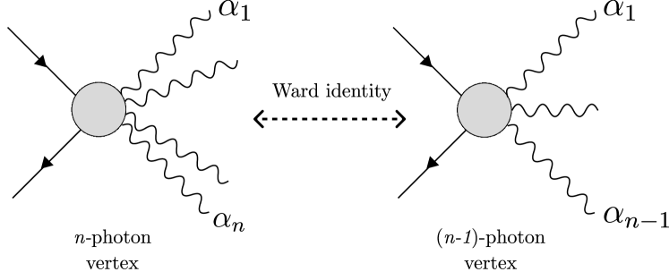
Figure 1: Ward identities of photon vertices with $n$ and $n-1$ photon lines

One can decompose the full photon vertex $\Gamma^{\alpha_{1}\cdots\alpha_{n}}$ into the bare vertex $\gamma^{\alpha_{1}\cdots\alpha_{n}}$ and the correction part $\Lambda^{\alpha_{1}\cdots\alpha_{n}}$ originating from the many-body effects:

$$\Gamma^{\alpha_{1}\cdots\alpha_{n}}=\gamma^{\alpha_{1}\cdots\alpha_{n}}+\Lambda^{\alpha_{1}\cdots\alpha_{n}}.$$ (10)

To give definitions of these quantities, let us introduce the action $S_{0}[A_{\mu},\bar{\psi},\psi]$ for the noninteracting limit that is also invariant under the local $U(1)$ gauge transformation in Eq. (3). The free Green function $G_{0,A}(x,y)$ in the presence of gauge field is defined by

$$G_{0,A}(x,y)$$

$$=-\frac{1}{Z_{0,A}}\int\mathcal{D}\bar{\psi}\mathcal{D}\psi\psi(x)\bar{\psi}(y)\exp[-S_{0}[A_{\mu},\bar{\psi},\psi]],$$ (11)

where $Z_{0,A}=\int\mathcal{D}\bar{\psi}\mathcal{D}\psi\exp[-S_{0}[A_{\mu},\bar{\psi},\psi]]$. The bare vertices are defined by

$$\gamma {}^{\alpha_{1}\cdots\alpha_{n}}(x,y,w_{1},\cdots,w_{n})$$

$$=(-1)^{n-1}\left.\left(\prod_{i=1}^{n}\functionalderivative{A_{\alpha_{i}}(w_{i})}\right)G_{0,A}^{-1}(x,y)\right|_{A=0},$$ (12)

which by themselves satisfy the Ward identity for bare one-photon vertices

$$\gamma^{\mu}(k,q)q_{\mu}=G_{0}^{-1}(k+q)\tau_{3}-\tau_{3}G_{0}^{-1}(k)$$ (13)

and for bare multi-photon vertices:

$$(q_{n})_{\alpha_{n}} \gamma^{\alpha_{1}\cdots\alpha_{n}}(k,q_{1},\cdots,q_{n})$$

$$= \tau_{3}\gamma^{\alpha_{1}\cdots\alpha_{n-1}}(k,q_{1},\cdots,q_{n-1})$$

$$-\gamma^{\alpha_{1}\cdots\alpha_{n-1}}(k+q_{n},q_{1},\cdots,q_{n-1})\tau_{3}.$$ (14)

The Dyson equation

$$G_{A}^{-1}(x,y)=G_{0,A}^{-1}(x,y)-\Sigma_{A}(x,y)$$ (15)

relates the full Green function $G_{A}(x,y)$ and the bare Green function $G_{0,A}(x,y)$, which in turn defines the self-energy $\Sigma_{A}(x,y)$. We define the correction part for the photon vertex by

$$\Lambda {}^{\alpha_{1}\cdots\alpha_{n}}(x,y,w_{1},\cdots,w_{n})$$

$$=(-1)^{n}\left.\left(\prod_{i=1}^{n}\functionalderivative{A_{\alpha_{i}}(w_{i})}\right)\Sigma_{A}(x,y)\right|_{A=0},$$ (16)

which satisfies the Ward identity for the correction part:

$$(q_{n})_{\alpha_{n}} \Lambda^{\alpha_{1}\cdots\alpha_{n}}(k,q_{1},\cdots,q_{n})$$

$$= \tau_{3}\Lambda^{\alpha_{1}\cdots\alpha_{n-1}}(k,q_{1},\cdots,q_{n-1})$$

$$-\Lambda^{\alpha_{1}\cdots\alpha_{n-1}}(k+q_{n},q_{1},\cdots,q_{n-1})\tau_{3}.$$ (17)

II.2 Diagrammatic representation of the electromagnetic response kernel

Here, we examine how the full photon vertex and the bare photon vertex, defined in the previous section, appear in the expression of the response kernel. We summarize the Feynman rules for the electromagnetic response kernel in many-body systems.

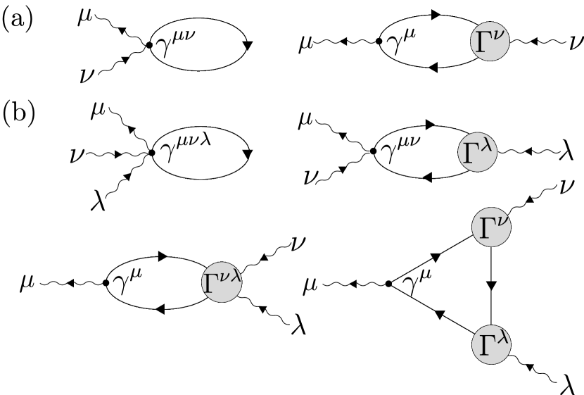
Figure 2: The diagrammatic representation of the electromagnetic response kernels. (a) The linear response kernel $K^{\mu\nu}$. (b) The second-order response kernel $K^{\mu\nu\lambda}$.

Let us assume that the microscopic action of a system with a background gauge field can be decomposed as

$$S[A_{\mu},\bar{\psi},\psi]=S_{0}[A_{\mu},\bar{\psi},\psi]+S_{\mathrm{int}}[\bar{\psi},\psi].$$ (18)

Here, the first term represents the noninteracting limit of the action and the second term represents the interaction between electrons. Crucially, we assume that the interactions do not depend on the gauge field. Under this assumption, the current is defined as

$$J_{A}^{\mu}(x)=-\functionalderivative{S_{0}[A_{\mu},\bar{\psi},\psi]}{A_{\mu}(x)}.$$ (19)

The noninteracting action can be expressed in terms of the bare Green function $G_{0,A}(x,y)$ as

$$S_{0}[A_{\mu},\bar{\psi},\psi]=-\frac{1}{2}\bar{\psi}(\overline{w}_{1})G_{0,A}^{-1}(\overline{w}_{1},\overline{w}_{2})\psi(\overline{w}_{2}).$$ (20)

The factor $1/2$ represents the particle-hole doubling due to the Nambu basis. Here and hereafter, we use the abbreviation for integral

$$f(\overline{x})g(\overline{x})=\int d^{4}xf(x)g(x).$$ (21)

Namely, a pair of overlined variables implies an integration over those variables.

The current can be expressed as

$$J_{A}^{\mu}(x)=\frac{1}{2}\bar{\psi}(\overline{w}_{1})\gamma_{A}^{\mu}(\overline{w}_{1},\overline{w}_{2},x)\psi(\overline{w}_{2})$$ (22)

using the generalized bare photon vertex $\gamma_{A}^{\mu}$ defined by

$$\gamma_{A}^{\mu}(w_{1},w_{2},x)=\functionalderivative{G_{0,A}^{-1}(w_{1},w_{2})}{A_{\mu}(x)}.$$ (23)

Therefore, the expectation value of the current can be expressed in terms of the Green function as

$$\expectationvalue{J_{A}^{\mu}(x)}=\frac{1}{2}\mathrm{Tr}\left[\gamma_{A}^{\mu}(\overline{w}_{1},\overline{w}_{2},x)G_{A}(\overline{w}_{2},\overline{w}_{1})\right].$$ (24)

Expanding this into the series of the gauge field $A$, we find

$$\expectationvalue{J_{A}^{\mu}(x)} =\sum_{n=0}^{\infty}\frac{1}{n!}K^{\mu\alpha_{1}\cdots\alpha_{n}}(x,\overline{w}_{1},\cdots,\overline{w}_{n})$$

$$\qquad\qquad\times A_{\alpha_{1}}(\overline{w}_{1})\cdots A_{\alpha_{n}}(\overline{w}_{n}).$$ (25)

Thus the $n$-th order electromagnetic response kernel is obtained by $n$-th functional derivative of $\expectationvalue{J_{A}^{\mu}(x)}$ with respect to the gauge field $A$:

$$K^{\mu\alpha_{1}\cdots\alpha_{n}}(x,y_{1},\cdots,y_{n})=\left.\frac{\delta^{n}\langle J_{A}^{\mu}(x)\rangle}{\delta A_{\alpha_{1}}(y_{1})\cdots\delta A_{\alpha_{n}}(y_{n})}\right|_{A=0}.$$ (26)

For example, the linear electromagnetic response kernel is defined as

$$K^{\mu\nu}(x,y)=\left.\functionalderivative{\expectationvalue{J_{A}^{\mu}(x)}}{A_{\nu}(y)}\right|_{A=0},$$ (27)

and the second-order response kernel is given by

$$K^{\mu\nu\lambda}(x,y,z)=\left.\frac{\delta^{2}\expectationvalue{J_{A}^{\mu}(x)}}{\delta A_{\nu}(y)\delta A_{\lambda}(z)}\right|_{A=0}.$$ (28)

Plugging Eq. (24) into Eq. (27), we obtain the explicit form

$$K^{\mu\nu}(x,y) =\frac{1}{2}\left.\mathrm{Tr}\big{[}\gamma_{A}^{\mu}(\overline{w}_{1},\overline{w}_{2},x)\functionalderivative{G_{A}(\overline{w}_{2},\overline{w}_{1})}{A_{\nu}(y)}+\functionalderivative{\gamma_{A}^{\mu}(\overline{w}_{1},\overline{w}_{2},x)}{A_{\nu}(y)}G_{A}(\overline{w}_{2},\overline{w}_{1})\big{]}\right|_{A=0}$$

$$=\frac{1}{2}\bigg{(}-\mathrm{Tr}\big{[}\gamma^{\mu}(\overline{w}_{1},\overline{w}_{2},x)G(\overline{w}_{2},\overline{w}_{3})\Gamma^{\nu}(\overline{w}_{3},\overline{w}_{4},y)G(\overline{w}_{4},\overline{w}_{1})\big{]}-\mathrm{Tr}\big{[}\gamma^{\mu\nu}(\overline{w}_{1},\overline{w}_{2},x,y)G(\overline{w}_{2},\overline{w}_{1})\big{]}\bigg{)}.$$ (29)

In the derivation, we used

$$\left.\functionalderivative{G_{A}(w_{2},w_{1})}{A_{\nu}(y)}\right|_{A=0} =-\left.G_{A}(w_{2},\overline{w}_{3})\functionalderivative{G_{A}^{-1}(\overline{w}_{3},\overline{w}_{4})}{A_{\nu}(y)}G_{A}(\overline{w}_{4},w_{1})\right|_{A=0}=-G(w_{2},\overline{w}_{3})\Gamma^{\nu}(\overline{w}_{3},\overline{w}_{4},y)G(\overline{w}_{4},w_{1})$$ (30)

and

$$\left.\functionalderivative{\gamma_{A}^{\mu}(w_{1},w_{2},x)}{A_{\nu}(y)}\right|_{A=0} =\left.\frac{\delta^{2}G_{0,A}^{-1}(w_{1},w_{2})}{\delta A_{\mu}(x)\delta A_{\nu}(y)}\right|_{A=0}=-\gamma^{\mu\nu}(w_{1},w_{2},x,y),$$ (31)

and we defined the Green function without a gauge field as

$$G(x,y)=\left.G_{A}(x,y)\right|_{A=0}.$$ (32)

The Feynman diagrams for Eq. (29) can be illustrated as in Fig. 2(a).

Similarly, for the second-order response kernel, we obtain

$$K^{\mu\nu\lambda}(x,y,z)=\frac{1}{2}\bigg{(} \frac{1}{2}\mathrm{Tr}\big{[}\gamma^{\mu\nu\lambda}(\overline{w}_{1},\overline{w}_{2},x,y,z)G(\overline{w}_{2},\overline{w}_{1})\big{]}+\mathrm{Tr}\big{[}\gamma^{\mu\nu}(\overline{w}_{1},\overline{w}_{2},x,y)G(\overline{w}_{2},\overline{w}_{3})\Gamma^{\lambda}(\overline{w}_{3},\overline{w}_{4},z)G(\overline{w}_{4},\overline{w_{1}})\big{]}$$

$$\qquad+\frac{1}{2}\mathrm{Tr}\big{[}\gamma^{\mu}(\overline{w}_{1},\overline{w_{2}},x)G(\overline{w}_{2},\overline{w}_{3})\Gamma^{\nu\lambda}(\overline{w}_{3},\overline{w}_{4},y,z)G(\overline{w}_{4},\overline{w}_{1})\big{]}$$

$$\qquad+\mathrm{Tr}\big{[}\gamma^{\mu}(\overline{w}_{1},\overline{w}_{2},x)G(\overline{w}_{2},\overline{w}_{3})\Gamma^{\lambda}(\overline{w}_{3},\overline{w}_{4},z)G(\overline{w}_{4},\overline{w}_{5})\Gamma^{\nu}(\overline{w}_{5},\overline{w}_{6},y)G(\overline{w}_{6},\overline{w}_{1})\big{]}$$

$$\qquad+[(\nu,y)\leftrightarrow(\lambda,z)]\bigg{)}.$$ (33)

The corresponding Feynman diagrams are presented in Fig. 2(b). A higher-order response kernel can also be derived systematically.

Assuming translational symmetry in the system, one can switch to momentum space by Fourier transformation. The Fourier transformation of Eq. (25) is given by

$$\expectationvalue{\hat{J}_{A}^{\mu}(q)}=\sum_{n=0}^{\infty}\frac{1}{n!} \delta(q-\sum_{i=1}^{n}q_{i})K^{\mu\alpha_{1}\cdots\alpha_{n}}(q_{1},\cdots,q_{n})$$

$$\times A_{\alpha_{1}}(q_{1})\cdots A_{\alpha_{n}}(q_{n})$$ (34)

and the $n$-th order response kernel in momentum space is defined. Note that the response kernel has an intrinsic permutation symmetry [32]:

$$K^{\mu\alpha_{p(1)}\cdots\alpha_{p(n)}}(q_{p(1)},\cdots,q_{p(n)})=K^{\mu\alpha_{1}\cdots\alpha_{n}}(q_{1},\cdots,q_{n})$$ (35)

for any permutation $p$.

Table 1: Feynman rules for the electromagnetic response kernel in interacting systems.

Diagrams		value
photon line		$1$
electron line		$G$
$(m+1)$-photon output vertex		$\frac{1}{m!}\gamma^{\mu\alpha_{i_{1}}\cdots\alpha_{i_{m}}}$
$m$-photon input vertex		$\frac{1}{m!}\Gamma^{\alpha_{i_{1}}\cdots\alpha_{i_{m}}}$

Continuing the above calculations, we obtain the following Feynman rules for $K^{\mu\alpha_{1}\cdots\alpha_{n}}(q_{1},\cdots,q_{n})$:

1. Each diagram contains $n+1$ external photon lines.

   1. Among them, one is the outgoing line $(\mu,q_{1}+\cdots+q_{n})$ and the others are incoming lines $(\alpha_{i},q_{i})$. Whole diagrams are symmetric about the $n$ input lines.

   2. A vertex containing the outgoing photon line is called an output vertex. All the others are called input vertices.

2. Internal electron lines form a loop.

3. The entire diagram comes with a factor of $(-1)^{n}/2$.

For example, the linear response kernel is given by

$$K^{\mu\nu}(q) =\frac{1}{2}\bigg{(}-\mathrm{Tr}\big{[}\gamma^{\mu}(\overline{k}+q,-q)G(\overline{k}+q)\Gamma^{\nu}(\overline{k},q)G(\overline{k})\big{]}-\mathrm{Tr}\big{[}\gamma^{\mu\nu}(\overline{k},-q,q)G(\overline{k})\big{]}\bigg{)},$$ (36)

and the second-order response kernel is

$$K^{\mu\nu\lambda}(q_{1},q_{2}) =\frac{1}{2}\bigg{(}\frac{1}{2}\mathrm{Tr}\big{[}\gamma^{\mu\nu\lambda}(\overline{k},-q,q_{1},q_{2})G(\overline{k})\big{]}+\mathrm{Tr}\big{[}\gamma^{\mu\nu}(\overline{k}+q_{2},-q,q_{1})G(\overline{k}+q_{2})\Gamma^{\lambda}(\overline{k},q_{2})G(\overline{k})\big{]}$$

$$\qquad+\frac{1}{2}\mathrm{Tr}\big{[}\gamma^{\mu}(\overline{k}+q,-q)G(\overline{k}+q)\Gamma^{\nu\lambda}(\overline{k},q_{1},q_{2})G(\overline{k})\big{]}$$

$$\qquad+\mathrm{Tr}\big{[}\gamma^{\mu}(\overline{k}+q,-q)G(\overline{k}+q)\Gamma^{\lambda}(\overline{k}+q_{1},q_{2})G(\overline{k}+q_{1})\Gamma^{\nu}(\overline{k},q_{1})G(\overline{k})\big{]}+[(\nu,q_{1})\leftrightarrow(\lambda,q_{2})]\bigg{)}.$$ (37)

These results agree with the Fourier transform of Eqs. (29) and (33). The explicit formula for the $n$-th order response kernel can also be obtained by drawing all the diagrams that obey these Feynman rules and assigning the values corresponding to each diagram summarized in Table 1.

II.3 Gauge invariance of response kernel

In this section, we demonstrate the gauge invariance of the electromagnetic response kernel obtained above based on the Ward identity.

The gauge transformation

$$A_{\alpha_{i}}(q_{i})\to A_{\alpha_{i}}(q_{i})-i(q_{i})_{\alpha_{i}}\theta(q_{i})$$ (38)

generates various additional terms in the expression of the current response in Eq. (34). For the gauge invariance, all these terms must vanish. This requires

$$K^{\mu\alpha_{1}\cdots\alpha_{n}}(q_{1},\cdots,q_{n})(q_{n})_{\alpha_{n}}=0.$$ (39)

Let us show that the electromagnetic response kernel constructed above satisfies this condition. For example, the linear response kernel in Eq. (36) satisfies

$$2K^{\mu\nu}(q)q_{\nu} =-\mathrm{Tr}\big{[}\gamma^{\mu}(\overline{k}+q,-q)G(\overline{k}+q)\Gamma^{\nu}(\overline{k},q)q_{\nu}G(\overline{k})+\gamma^{\mu\nu}(\overline{k},-q,q)q_{\nu}G(\overline{k})\big{]}$$

$$=-\mathrm{Tr}\big{[}\gamma^{\mu}(\overline{k}+q,-q)G(\overline{k}+q)\left(G^{-1}(\overline{k}+q)\tau_{3}-\tau_{3}G^{-1}(\overline{k})\right)G(\overline{k})\big{]}$$

$$\qquad-\mathrm{Tr}\big{[}\left(\tau_{3}\gamma^{\mu}(\overline{k},-q)-\gamma^{\mu}(\overline{k}+q,-q)\tau_{3}\right)G(\overline{k})\big{]}$$

$$=0.$$ (40)

In going to the second line, we used the Ward identity for the bare two-photon vertices

$$\gamma^{\mu\nu}(k,q_{1},q_{2})(q_{2})_{\nu}=\tau_{3}\gamma^{\mu}(k,q_{1})-\gamma^{\mu}(k+q_{2},q_{1})\tau_{3}$$ (41)

and the Ward identity for the full one-photon vertices

$$\Gamma^{\nu}(k,q)q_{\nu}=G^{-1}(k+q)\tau_{3}-\tau_{3}G^{-1}(k).$$ (42)

Also, for the second-order response kernel,

$$2K^{\mu\nu\lambda}(q_{1},q_{2})(q_{2})_{\lambda} =\mathrm{Tr}\big{[}\gamma^{\mu\nu\lambda}(\overline{k},-q,q_{1},q_{2})(q_{2})_{\lambda}G(\overline{k})\big{]}+\mathrm{Tr}\big{[}\gamma^{\mu\nu}(\overline{k}+q_{2},-q,q_{1})G(\overline{k}+q_{2})\Gamma^{\lambda}(\overline{k},q_{2})(q_{2})_{\lambda}G(\overline{k})\big{]}$$

$$\quad+\mathrm{Tr}\big{[}\gamma^{\mu\lambda}(\overline{k}+q_{1},-q,q_{2})(q_{2})_{\lambda}G(\overline{k}+q_{1})\Gamma^{\nu}(\overline{k},q_{1})G(\overline{k})\big{]}$$

$$\quad+\mathrm{Tr}\big{[}\gamma^{\mu}(\overline{k}+q,-q)G(\overline{k}+q)\Gamma^{\nu\lambda}(\overline{k},q_{1},q_{2})(q_{2})_{\lambda}G(\overline{k})\big{]}$$

$$\quad+\mathrm{Tr}\big{[}\gamma^{\mu}(\overline{k}+q,-q)G(\overline{k}+q)\Gamma^{\lambda}(\overline{k}+q_{1},q_{2})(q_{2})_{\lambda}G(\overline{k}+q_{1})\Gamma^{\nu}(\overline{k},q_{1})G(\overline{k})\big{]}$$

$$\quad+\mathrm{Tr}\big{[}\gamma^{\mu}(\overline{k}+q,-q)G(\overline{k}+q)\Gamma^{\nu}(\overline{k}+q_{2},q_{1})G(\overline{k}+q_{2})\Gamma^{\lambda}(\overline{k},q_{2})(q_{2})_{\lambda}G(\overline{k})\big{]}$$

$$=\mathrm{Tr}\big{[}\big{(}\tau_{3}\gamma^{\mu\nu}(\overline{k},-q,q_{1})-\gamma^{\mu\nu}(\overline{k}+q_{2},-q,q_{1})\tau_{3}\big{)}G(\overline{k})\big{]}$$

$$\quad+\mathrm{Tr}\big{[}\gamma^{\mu\nu}(\overline{k}+q_{2},-q,q_{1})G(\overline{k}+q_{2})(G^{-1}(\overline{k}+q_{2})\tau_{3}-\tau_{3}G^{-1}(\overline{k}))G(\overline{k})\big{]}$$

$$\quad+\mathrm{Tr}\big{[}\big{(}\tau_{3}\gamma^{\mu}(\overline{k}+q_{1},-q)-\gamma^{\mu}(\overline{k}+q,-q)\tau_{3}\big{)}G(\overline{k}+q_{1})\Gamma^{\nu}(\overline{k},q_{1})G(\overline{k})\big{]}$$

$$\quad+\mathrm{Tr}\big{[}\gamma^{\mu}(\overline{k}+q,-q)G(\overline{k}+q)\big{(}\tau_{3}\Gamma^{\nu}(\overline{k},q_{1})-\Gamma^{\nu}(\overline{k}+q_{2},q_{1})\tau_{3}\big{)}G(\overline{k})\big{]}$$

$$\quad+\mathrm{Tr}\big{[}\gamma^{\mu}(\overline{k}+q,-q)G(\overline{k}+q)\big{(}G^{-1}(\overline{k}+q)\tau_{3}-\tau_{3}G^{-1}(\overline{k}+q_{1})\big{)}G(\overline{k}+q_{1})\Gamma^{\nu}(\overline{k},q_{1})G(\overline{k})\big{]}$$

$$\quad+\mathrm{Tr}\big{[}\gamma^{\mu}(\overline{k}+q,-q)G(\overline{k}+q)\Gamma^{\nu}(\overline{k}+q_{2},q_{1})G(\overline{k}+q_{2})\big{(}G^{-1}(\overline{k}+q_{2})\tau_{3}-\tau_{3}G^{-1}(\overline{k})\big{)}G(\overline{k})\big{]}$$

$$=0.$$ (43)

Even for higher-order responses, one can prove their gauge invariance in the same way regardless of the specific details of the model.

II.4 Optical responses in many-body systems

Next, we discuss the optical response as the $\bm{q}\to\bm{0}$ limit of the electromagnetic response. For this purpose, we assume a spatially uniform and time-dependent electric field $\bm{E}$. Since the gauge invariance of electromagnetic responses has been confirmed, we can fix the gauge to the one convenient for our purpose

$$A_{0}(q)=0,~\bm{A}(q)=\frac{\bm{E}(i\Omega)}{i(i\Omega)},$$ (44)

which is called the velocity gauge [3, 33].

In this case, the $n$-th order current in Eq. (34) can be rewritten as

$$\langle J_{A}^{\mu}(i\Omega)\rangle=\sum_{n=0}^{\infty}\frac{1}{n!}\sigma^{\mu\alpha_{1}\cdots\alpha_{n}}(i\Omega_{1},\cdots,i\Omega_{n})$$

$$\qquad\times\delta(i\Omega-\sum_{j=1}^{n}i\Omega_{j})E_{\alpha_{1}}(i\Omega_{1})\cdots E_{\alpha_{n}}(i\Omega_{n}),$$ (45)

where the $n$-th order optical conductivity is defined as

$$\sigma^{\mu\alpha_{1}\cdots\alpha_{n}}(i\Omega_{1},\cdots,i\Omega_{n})$$

$$=\bigg{(}\prod_{j=1}^{n}\frac{1}{i(i\Omega_{j})}\bigg{)}\left.K^{\mu\alpha_{1}\cdots\alpha_{n}}(q_{1},\cdots,q_{n})\right|_{\bm{q_{i}=0}}.$$ (46)

The frequency response of the system is obtained via analytic continuation $i\Omega_{i}\to\omega_{i}+i\eta$, where $\eta$ is an infinitesimal positive parameter.

III Applications to superconductors

In this section, we apply the electromagnetic response theory developed in Sec. II to superconductors.

III.1 The mean-field theory of superconductors

First, we review the mean-field theory of superconductors. We assume the microscopic action $S[A_{\mu},\bar{\psi},\psi]$ possesses local $U(1)$ symmetry and the interaction part $S_{\mathrm{int}}[\bar{\psi},\psi]$ does not depend on the gauge field as shown in Eqs. (4) and (18). Under these assumptions, the microscopic interaction between electrons should take the form

$$\hat{H}_{\mathrm{int}}=-\frac{1}{2}\sum_{\bm{x,y}}\sum_{\alpha\beta\gamma\delta}V^{\alpha\beta\gamma\delta}(\bm{x-y})\hat{c}_{\bm{x}\alpha}^{\dagger}\hat{c}_{\bm{y}\beta}^{\dagger}\hat{c}_{\bm{y}\gamma}\hat{c}_{\bm{x}\delta},$$ (47)

where indices $\alpha$,$\beta$,$\gamma$, and $\delta$ represent internal degrees of freedom. Due to the anticommutation relation of the electrons, $V^{\beta\alpha\delta\gamma}(\bm{y-x})=V^{\alpha\beta\gamma\delta}(\bm{x-y})$ should hold. In momentum space, this interaction can be expressed as

$$\hat{H}_{\mathrm{int}}=-\frac{1}{2N} \sum_{\bm{k,p,q}}\sum_{\alpha\beta\gamma\delta}V^{\alpha\beta\gamma\delta}(\bm{k-p})$$

$$\times\hat{c}_{\bm{k+q}\alpha}^{\dagger}\hat{c}_{\bm{-k+q}\beta}^{\dagger}\hat{c}_{\bm{-p+q}\gamma}\hat{c}_{\bm{p+q}\delta},$$ (48)

where $V^{\alpha\beta\gamma\delta}(\bm{k-p})$ is the Fourier transform of $V^{\alpha\beta\gamma\delta}(\bm{x-y})$. Applying the mean-field approximation in the Cooper channel, we define the gap function as

$$[\Delta(\bm{k})]_{\alpha\beta}=-\frac{1}{N} \sum_{\bm{p}}\sum_{\gamma\delta}V^{\alpha\beta\gamma\delta}(\bm{k-p})\langle\hat{c}_{\bm{-p}\gamma}\hat{c}_{\bm{p}\delta}\rangle.$$ (49)

With this approximation, the interaction term is simplified to

$$\hat{H}_{\mathrm{int}}\to\frac{1}{2}\sum_{k}\sum_{\alpha\beta}\bigg{(}\hat{c}_{\bm{k}\alpha}^{\dagger}[\Delta(\bm{k})]_{\alpha\beta}\hat{c}_{\bm{-k}\beta}^{\dagger}+h.c.\bigg{)}.$$ (50)

Adding this to the normal-state Hamiltonian

$$\hat{H}_{N}=\sum_{\bm{k}}\sum_{\alpha\beta}\hat{c}_{\bm{k}\alpha}^{\dagger}[H_{N}(\bm{k})]_{\alpha\beta}\hat{c}_{\bm{k}\beta},$$ (51)

we obtain the mean-field Hamiltonian in the Bogoliubov-de Gennes (BdG) form:

$$\hat{H}_{\mathrm{MF}}=\frac{1}{2}\sum_{\bm{k}}\hat{\psi}_{\bm{k}}^{\dagger}H_{\mathrm{BdG}}(\bm{k})\hat{\psi}_{\bm{k}},$$ (52)

where

$$H_{\mathrm{BdG}}(\bm{k})=\begin{pmatrix}H_{N}(\bm{k})&\Delta(\bm{k})\\ \Delta^{\dagger}(\bm{k})&-[H_{N}(-\bm{k})]^{T}\end{pmatrix},$$ (53)

is the BdG Hamiltonian and

$$\hat{\psi}_{\bm{k}}=\begin{pmatrix}\hat{\bm{c}}_{\bm{k}}\\ (\hat{\bm{c}}_{\bm{-k}}^{\dagger})^{T}\end{pmatrix}$$ (54)

is the Nambu spinor. This mean-field Hamiltonian no longer has $U(1)$ symmetry.

Next, we introduce the gauge field $A_{\mu}$ into the system to discuss electromagnetic responses later. In general, the gauge field breaks translational symmetry, so it is necessary to discuss the mean-field theory of superconductors in real space. Since we assume the gauge field does not affect the interaction term, the interaction in the presence of the gauge field remains identical to Eq. (47). Under the mean-field approximation in the Cooper channel, the real space representation of the gap function is defined as

$$[\Delta_{A}(\bm{x,y})]_{\alpha\beta}=-\sum_{\gamma\delta}V^{\alpha\beta\gamma\delta}(\bm{x-y})\langle\hat{c}_{\bm{y}\gamma}\hat{c}_{\bm{x}\delta}\rangle.$$ (55)

This gap function depends on $A_{\mu}$, as the gauge field modifies the normal-state Hamiltonian $\hat{H}_{N}\to\hat{H}_{N,A}$, and consequently alters the expectation value $\langle\hat{c}_{\bm{y}\gamma}\hat{c}_{\bm{x}\delta}\rangle$. The expectation value can be rewritten using the Green function as

$$\langle\hat{c}_{\bm{y}\gamma}\hat{c}_{\bm{x}\delta}\rangle =-\langle T_{\tau}\hat{c}_{\bm{x}\delta}(0^{-})\hat{c}_{\bm{y}\gamma}(0)\rangle$$

$$=\mathrm{Tr}\big{[}P_{\gamma\delta}G_{A}(\bm{x,y};0^{-})\big{]}.$$ (56)

where we defined the matrices

$$P_{\gamma\delta}=\begin{pmatrix}O&O\\ E_{\gamma\delta}&O\end{pmatrix}$$ (57)

and $[E_{\gamma\delta}]_{ab}=\delta_{a\gamma}\delta_{b\delta}$. The self-energy is given by

$$\Sigma_{A}(x,y)=\begin{pmatrix}O&\Delta_{A}(x,y)\\ \Delta_{A}^{\dagger}(y,x)&O\end{pmatrix}$$ (58)

where

$$[\Delta_{A}(x,y)]_{\alpha\beta}=-\sum_{\gamma\delta}V^{\alpha\beta\gamma\delta}(x-y)\mathrm{Tr}\big{[}P_{\gamma\delta}G_{A}(x,y)\big{]}$$ (59)

and $V^{\alpha\beta\gamma\delta}(x-y)=V^{\alpha\beta\gamma\delta}(\bm{x-y})\delta(x_{0}-y_{0}-0^{-})$.

III.2 The Ward identities under the mean-field approximation

We now turn to the discussion of electromagnetic responses. While it may seem straightforward to apply the gauge-invariant theory for many-body systems summarized earlier, it is necessary to ensure one crucial condition is met. Namely, we must examine whether the Ward identities are consistent with the approximation employed.

The whole Ward identities for photon vertices are derived by the functional derivatives of Eq. (7). Plugging the Dyson equation in Eq.(15) into Eq. (7), we obtain the relation that should hold between the self-energies:

$$\partial_{z^{\mu}}\functionalderivative{\Sigma_{A}(x,y)}{A_{\mu}(z)}$$

$$=i\delta(x-z)\tau_{3}\Sigma_{A}(x,y)-i\Sigma_{A}(x,y)\tau_{3}\delta(y-z).$$ (60)

Since the self-energy of superconductors is given by Eq. (58), the gap function should satisfy

$$\partial_{z^{\mu}}\functionalderivative{\Delta_{A}(x,y)}{A_{\mu}(z)}$$

$$=i\Delta_{A}(x,y)\delta(y-z)+i\Delta_{A}(x,y)\delta(x-z).$$ (61)

We can prove that this relation is compatible with the adopted approximations as follows, using the definition of the gap function in Eq. (59):

$$\partial_{z^{\mu}}\functionalderivative{[\Delta_{A}(x,y)]_{\alpha\beta}}{A_{\mu}(z)}=\sum_{\gamma\delta}V^{\alpha\beta\gamma\delta}(x-y)\partial_{z^{\mu}}\mathrm{Tr}\big{[}P_{\gamma\delta}G_{A}(x,\overline{x}^{\prime})\functionalderivative{G_{A}^{-1}(\overline{x}^{\prime},\overline{y}^{\prime})}{A_{\mu}(z)}G_{A}(\overline{y}^{\prime},y)\big{]}$$

$$=\sum_{\delta\gamma}V^{\alpha\beta\gamma\delta}(x-y)\partial_{z^{\mu}}\mathrm{Tr}\big{[}P_{\gamma\delta}G_{A}(x,\overline{x}^{\prime})\big{(}i\delta(\overline{x}^{\prime}-z)\tau_{3}G_{A}^{-1}(\overline{x}^{\prime},\overline{y}^{\prime})-iG_{A}^{-1}(\overline{x}^{\prime},\overline{y}^{\prime})\tau_{3}\delta(\overline{y}^{\prime}-z)\big{)}G_{A}(\overline{y}^{\prime},y)\big{]}$$

$$=i[\Delta_{A}(x,y)]_{\alpha\beta}\delta(y-z)+i[\Delta_{A}(x,y)]_{\alpha\beta}\delta(x-z).$$ (62)

Therefore, it is possible to apply the electromagnetic theory above to superconductors which are originating from the microscopic interactions given by Eq. (47).

The calculation of electromagnetic responses can be done given the Green function, bare photon vertices, and full photon vertices. The Green function is obtained by

$$G^{-1}(k)=k_{0}\tau_{0}-H_{\mathrm{BdG}}(\bm{k}).$$ (63)

The bare and full photon vertices are obtained by definitions in Eqs. (12) and (6) and they automatically satisfy the Ward identities.

For instance, let us consider the photon vertices in the velocity gauge. Since the gauge field is introduced by the minimal coupling $\bm{k}\to\bm{k+A}$ for the electron part $H_{N}(\bm{k})$ and $\bm{-k}\to\bm{-k+A}$ for the hole part $H_{N}(-\bm{k})^{T}$, the bare $n$-photon vertices are given by

$$\gamma^{\alpha_{1}\cdots\alpha_{n}}(k)=\prod_{i=1}^{n}(-\tau_{3}\partial_{k_{i}})\begin{pmatrix}H_{N}(\bm{k})&\\ &-[H_{N}(-\bm{k})]^{T}\end{pmatrix}.$$ (64)

The full $n$-photon vertex $\Gamma^{\alpha_{1}\cdots\alpha_{n}}$ can be decomposed into the sum of the bare $n$-photon vertex $\gamma^{\alpha_{1}\dots\alpha_{n}}$ and the correction part $\Lambda^{\alpha_{1}\cdots\alpha_{n}}$ as shown in Eq. (10). The latter is obtained by the functional derivatives of the self-energy as in Eq. (16). Since the self-energy $\Sigma_{A}[G_{A}]$ is a functional of the Green function, the functional derivatives of the self-energy $\delta\Sigma/\delta A$ are related to the functional derivatives of the Green function $\delta G/\delta A$, which is again related to the full photon vertex. Therefore, the full photon vertices are given by the solutions to some integral equations.

The concrete form of the integral equation for the full photon vertex is determined by specifying the form of the self-energy. The Fock approximation leads to the Bethe-Salpeter equation for the correction part $\Lambda^{\mu}$, as we review in Sec. IV.1. However, this method has a subtlety associated to the diagonal components of the self-energy. Instead, we use the more precise expression of the self-energy in Eq. (59). The correction part of the full one-photon vertex $\Lambda^{\mu}=-\delta\Sigma_{A}/\delta A_{\mu}|_{A=0}$ is then directly calculated by the functional derivatives of the gap equation. This approach at the linear response level for BCS superconductors was called “consistent fluctuations of order parameters” (CFOP) method in Ref. [27], whose name reflects the fact that $\delta\Delta_{A}/\delta A_{\mu}$ represents the fluctuations of the gap function induced by the gauge field. Similar discussions of linear responses of BCS superconductors can be found in Refs. [34, 35]. Our derivation in this work is more general and is capable of handling responses of arbitrary order and more general superconductors as long as the microscopic interaction leading to the superconductivity takes the form of Eq. (47). Hence, we call our method generalized CFOP method and study the optical responses in superconductors in this framework. The concrete form of the integral equations for the full photon vertices are presented in Sec. IV. In Sec. IV.2, we will see that our method at the linear order level is equivalent to the random phase approximations addressed in Refs. [36, 37, 38] in the different context.

III.3 Finite momentum Cooper pairing

Our formulation can also be applied to the case where the Cooper pairs have a finite momentum $2\bm{Q}$. In this situation, the supreconducting gap is assumed to be

$$[\Delta(\bm{k})]_{\alpha\beta}=-\frac{1}{N} \sum_{\bm{p}}\sum_{\gamma\delta}V^{\alpha\beta\gamma\delta}(\bm{k-p})\langle\hat{c}_{\bm{-p+Q}\gamma}\hat{c}_{\bm{p+Q}\delta}\rangle,$$ (65)

and the interaction term is reduced to

$$\hat{H}_{\mathrm{int}}\to\sum_{\bm{k}}\sum_{\alpha\beta}\bigg{(}\hat{c}_{\bm{k+Q}\alpha}^{\dagger}[\Delta(\bm{k})]_{\alpha\beta}\hat{c}_{\bm{-k+Q}\beta}^{\dagger}+h.c.\bigg{)}.$$ (66)

The mean-field Hamiltonian is given by

$$\hat{H}_{\mathrm{MF}}=\frac{1}{2}\sum_{\bm{k}}(\hat{\psi}_{\bm{k}}^{\bm{Q}})^{\dagger}H_{\mathrm{BdG}}^{\bm{Q}}(\bm{k})\hat{\psi}_{\bm{k}}^{\bm{Q}},$$ (67)

where

$$H_{\mathrm{BdG}}^{\bm{Q}}(\bm{k})=\begin{pmatrix}H_{N}(\bm{k+Q})&\Delta(\bm{k})\\ \Delta^{\dagger}(\bm{k})&-H_{N}^{T}(\bm{-k+Q})\end{pmatrix}$$ (68)

and $\hat{\psi}_{\bm{k}}^{\bm{Q}}=(\hat{\bm{c}}_{\bm{k+Q}}^{T},\hat{\bm{c}}_{\bm{-k+Q}}^{\dagger})^{T}$.

To consider electromagnetic responses, we also present the case where the gauge field is present and translational symmetry is broken. The corresponding mean-field approximation in real space can be formulated by defining

$$\hat{\bm{c}}_{\bm{x}}^{\bm{Q}}=\hat{\bm{c}}_{\bm{x}}e^{-i\bm{Q}\cdot\bm{x}},(\hat{\bm{c}}_{\bm{x}}^{\bm{Q}})^{\dagger}=\hat{\bm{c}}_{\bm{x}}^{\dagger}e^{i\bm{Q}\cdot\bm{x}}.$$ (69)

The interaction term in Eq. (47) can be rewritten as

$$\hat{H}_{\mathrm{int}}=\sum_{\bm{x,y}}\sum_{\alpha\beta\gamma\delta}V^{\alpha\beta\gamma\delta}(\bm{x-y})(\hat{c}_{\bm{x}\alpha}^{\bm{Q}})^{\dagger}(\hat{c}_{\bm{y}\beta}^{\bm{Q}})^{\dagger}\hat{c}_{\bm{y}\gamma}^{\bm{Q}}\hat{c}_{\bm{x}\delta}^{\bm{Q}}.$$ (70)

The gap function in real space is defined by

$$[\Delta_{A}(\bm{x,y})]_{\alpha\beta}=\sum_{\gamma\delta}V^{\alpha\beta\gamma\delta}(\bm{x-y})\langle\hat{c}_{\bm{y}\gamma}^{\bm{Q}}\hat{c}_{\bm{x}\delta}^{\bm{Q}}\rangle.$$ (71)

Redefining the Nambu spinor in real space as

$$\hat{\psi}_{\bm{x}}^{\bm{Q}}=\begin{pmatrix}\hat{\bm{c}}_{\bm{x}}^{\bm{Q}}\\ ((\hat{\bm{c}}_{\bm{x}}^{\bm{Q}})^{\dagger})^{T}\end{pmatrix},$$ (72)

the self-energy is expressed in exactly the same form as Eqs. (58) and (59). Therefore, one can show the Ward identities are consistent with this approximation and discuss the gauge-invariant electromagnetic responses even in the situation where Cooper pairs have the finite momentum.

III.4 Spin rotational symmetry

If we further assume spin-singlet pairing and spin rotational symmetry, the size of the BdG Hamiltonian and the Nambu spinor can be halved. Since the introduction of the gauge field is independent of the spin operations, this dimensional reduction can be done even in the presence of the gauge field. For simplicity, we do not introduce the gauge field here.

We consider the degrees of freedom defined by sublattices $l=1,\cdots,n$ and spin $s={\uparrow},{\downarrow}$. The spin operator $\hat{S}^{i}_{\bm{x}l}$ on site $\bm{x}$ and sublattice $l$ is defined by

$$\hat{S}^{i}_{\bm{x}l}=\begin{pmatrix}\hat{c}_{\bm{x}l\uparrow}^{\dagger}&\hat{c}_{\bm{x}l\downarrow}^{\dagger}\end{pmatrix}\frac{\sigma_{i}}{2}\begin{pmatrix}\hat{c}_{\bm{x}l\uparrow}\\ \hat{c}_{\bm{x}l\downarrow}\end{pmatrix},$$ (73)

where $\sigma_{i}$ are the Pauli matrices that act on the spin space. The total spin operator is given by $\hat{S}^{i}=\sum_{\bm{x},l}\hat{S}^{i}_{\bm{x}l}$. The spin rotations are generated by $\hat{S}^{i}$, and a spin rotation about axis $\bm{n}$ by an angle $\phi$ is represented by

$$\hat{U}(\bm{n},\phi)=\exp(i\phi\bm{n}\cdot\hat{\bm{S}}).$$ (74)

This operation does not change the sublattice degrees of freedom.

Assuming spin rotational symmetry, the normal-state Hamiltonian takes the form

$$\hat{H}_{N}=\sum_{\bm{x,y}}\sum_{l,l^{\prime}}\sum_{s}\hat{c}_{\bm{x}ls}^{\dagger}[\tilde{H}_{N}(\bm{x,y})]_{ll^{\prime}}\hat{c}_{\bm{y}l^{\prime}s}.$$ (75)

If the interaction term is also invariant under spin rotation, it consists of the interactions such as spin-spin interaction

$$V_{S}^{l_{1}l_{2}l_{3}l_{4}}(\bm{x-y})(\bm{\sigma})_{s_{1}s_{4}}\cdot(\bm{\sigma})_{s_{2}s_{3}}$$ (76)

and density-density interaction

$$V_{n}^{l_{1}l_{2}l_{3}l_{4}}(\bm{x-y})(\sigma_{0})_{s_{1}s_{4}}(\sigma_{0})_{s_{2}s_{3}}.$$ (77)

For spin-singlet pairing, we assume the interaction term $\hat{H}_{\mathrm{int}}$ is represented by

$$V^{\alpha\beta\gamma\delta}(\bm{x-y})=V^{l_{1}l_{2}l_{3}l_{4}}(\bm{x-y})(i\sigma_{2})_{s_{1}s_{2}}(i\sigma_{2})^{\dagger}_{s_{3}s_{4}},$$ (78)

where $V^{l_{1}l_{2}l_{3}l_{4}}(\bm{x-y})=V^{l_{2}l_{1}l_{4}l_{3}}(\bm{y-x})$. This pairing interaction is invariant under spin rotation due to the equality

$$(i\sigma_{2})_{s_{1}s_{2}}(i\sigma_{2})^{\dagger}_{s_{3}s_{4}}$$

$$=-\frac{1}{2}\big{[}(\bm{\sigma})_{s_{1}s_{4}}\cdot(\bm{\sigma})_{s_{2}s_{3}}-(\sigma_{0})_{s_{1}s_{4}}(\sigma_{0})_{s_{2}s_{3}}\big{]}.$$ (79)

Therefore, this microscopic Hamiltonian for spin-singlet pairing possesses spin rotational symmetry:

$$\hat{U}(\bm{n},\phi)(\hat{H}_{N}+\hat{H}_{\mathrm{int}})\hat{U}^{\dagger}(\bm{n},\phi)=\hat{H}_{N}+\hat{H}_{\mathrm{int}}.$$ (80)

Performing mean-field approximation, we define the gap function as

$$[\Delta(\bm{x,y})]_{l_{1}s_{1},l_{2}s_{2}} =[\tilde{\Delta}(\bm{x,y})]_{l_{1}l_{2}}(i\sigma_{2})_{s_{1}s_{2}},$$ (81)

where

$$[\tilde{\Delta}(\bm{x,y})]_{l_{1}l_{2}} =-\sum_{l_{3}s_{3}l_{4}s_{4}}V^{l_{1}l_{2}l_{3}l_{4}}(\bm{x-y})$$

$$\qquad\times(i\sigma_{2})^{\dagger}_{s_{3}s_{4}}\langle\hat{c}_{\bm{y}l_{3}s_{3}}\hat{c}_{\bm{x}l_{4}s_{4}}\rangle,$$ (82)

and the mean-field Hamiltonian is written as

$$\hat{H}_{\mathrm{MF}}=\frac{1}{2}\sum_{\bm{x,y}}\hat{\psi}_{\bm{x}}^{\dagger}H_{\mathrm{BdG}}(\bm{x,y})\hat{\psi}_{\bm{y}},$$ (83)

where the BdG Hamiltonian is given by

$$H_{\mathrm{BdG}}(\bm{x,y})$$

$$=\begin{pmatrix}\tilde{H}_{N}(\bm{x,y})\otimes\sigma_{0}&\tilde{\Delta}(\bm{x,y})\otimes(i\sigma_{2})\\ \tilde{\Delta}^{\dagger}(\bm{y,x})\otimes(i\sigma_{2})^{\dagger}&-\tilde{H}_{N}^{T}(\bm{y,x})\otimes\sigma_{0}\end{pmatrix}.$$ (84)

Redefining the Nambu spinor as

$$\hat{\tilde{\psi}}_{\bm{x}}=\begin{pmatrix}\hat{\bm{c}}_{\bm{x}\uparrow}\\ (\hat{\bm{c}}_{\bm{x}\downarrow}^{\dagger})^{T}\end{pmatrix}$$ (85)

where $\hat{\bm{c}}_{\bm{x}s}=(\hat{c}_{\bm{x}1s},\cdots,\hat{c}_{\bm{x}ns})^{T}$, the mean-field Hamiltonian reduces to

$$\hat{H}_{\mathrm{MF}}=\sum_{\bm{x,y}}\hat{\tilde{\psi}}_{\bm{x}}^{\dagger}\tilde{H}_{\mathrm{BdG}}(\bm{x,y})\hat{\tilde{\psi}}_{\bm{y}}$$ (86)

with

$$\tilde{H}_{\mathrm{BdG}}(\bm{x,y})=\begin{pmatrix}\tilde{H}_{N}(\bm{x,y})&\tilde{\Delta}(\bm{x,y})\\ \tilde{\Delta}^{\dagger}(\bm{y,x})&-\tilde{H}_{N}^{T}(\bm{y,x})\end{pmatrix}.$$ (87)

This redefinition avoids the particle-hole doubling. The Green function and the self-energy are then defined as

$$\tilde{G}(x,y)=-\langle T_{\tau}\hat{\tilde{\psi}}(x)\hat{\tilde{\psi}}^{\dagger}(y)\rangle$$ (88)

$$\tilde{\Sigma}(x,y)=\begin{pmatrix}&\tilde{\Delta}(x,y)\\ \tilde{\Delta}^{\dagger}(y,x)&\end{pmatrix},$$ (89)

where

$$[\tilde{\Delta}(x,y)]_{l_{1}l_{2}}= -2\sum_{l_{3}l_{4}}V^{l_{1}l_{2}l_{3}l_{4}}(x-y)\mathrm{Tr}\big{[}P_{l_{3}l_{4}}\tilde{G}(x,y)\big{]}$$ (90)

and $V^{l_{1}l_{2}l_{3}l_{4}}(x-y)=V^{l_{1}l_{2}l_{3}l_{4}}(\bm{x-y})\delta(x_{0}-y_{0}-0^{-})$. This approach removes the $1/2$ factors often introduced in definitions of current and response kernels due to the particle-hole doubling.

IV Examples

In this section, we discuss electromagnetic responses of superconductors in several models. The first example clarifies the relation between the generalized CFOP method and previous studies [23, 34, 35, 27]. The second and third examples, which are multi-band $s$-wave superconductors and single-band $d$-wave superconductors, are used to demonstrate the significance of vertex corrections in optical response. Since all of these examples possess spin rotational symmetry and spin-singlet pairing is assumed, we omit all tildes, for example, in the Green function $\tilde{G}$ and the Nambu spinor $\tilde{\psi}$.

IV.1 BCS single-band superconductors

In the BCS theory, the internal degree of freedom is given by spin $s={\uparrow},{\downarrow}$. The interaction between electrons can be written as

$$V^{s_{1}s_{2}s_{3}s_{4}}(\bm{x-y})=\frac{1}{2}V(\bm{x-y})(i\sigma_{2})_{s_{1},s_{2}}(i\sigma_{2})^{\dagger}_{s_{3},s_{4}},$$ (91)

where $V(\bm{x-y})$ is real function. Then, the self-energy in Eq. (59) of this superconductor is given by

$$\Sigma_{A}(x,y)=\begin{pmatrix}&\Delta_{A}(x,y)\\ \Delta_{A}^{\dagger}(y,x)&\end{pmatrix},$$ (92)

$$\Delta_{A}(x,y)=-V(x-y)\mathrm{Tr}\big{[}PG_{A}(x,y)\big{]}.$$ (93)

Instead of Eq. (93), one often uses the Fock approximation to the self-energy illustrated in Fig. 3(a):

$$\Sigma_{A}(x,y)=V(x-y)\tau_{3}G_{A}(x,y)\tau_{3},$$ (94)

which, combined with Eqs. (6) and (15), gives the full one-photon vertex:

$$\Gamma^{\mu}(x,y,z)=\gamma^{\mu}(x,y,z)-\left.\functionalderivative{\Sigma_{A}(x,y)}{A_{\mu}(z)}\right|_{A=0}$$

$$=\gamma^{\mu}(x,y,z)$$

$$\quad+V(x-y)\tau_{3}G(x,\overline{x}^{\prime})\Gamma^{\mu}(\overline{x}^{\prime},\overline{y}^{\prime},z)G(\overline{y}^{\prime},y)\tau_{3}.$$ (95)

See Fig. 3(b) for the diagrammatic expression. Performing the Fourier transform, we obtain the Bethe-Salpeter equation [23]:

$$\Gamma^{\mu}(k,q)=\gamma^{\mu}(k,q)+V(k-\overline{p})\tau_{3}G(\overline{p}+q)\Gamma^{\mu}(\overline{p},q)G(\overline{p})\tau_{3}.$$ (96)

While Nambu [23] argued only the linear electromagnetic responses, our method can also derive its nonlinear extension, which will be discussed in Appendix B.

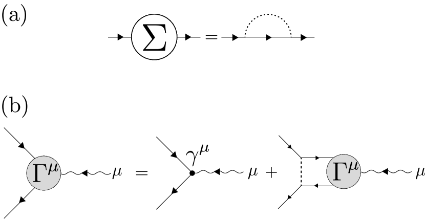
Figure 3: The Green function method of BCS superconductors. (a) The Fock approximation to the self-energy. The dotted line corresponds to the microscopic interaction between electrons $V$. (b) The Bethe-Salpeter equation. The Bethe-Salpeter equation is the ladder approximation to the bare one-photon vertex.

It should be noted that Eq. (94) differs from Eq. (93) in its diagonal component. This mismatch is often justified from the fact that the diagonal components of the self-energy only affect the band dispersion of the normal state and do not change the superconducting gap. However, the diagonal components of the self-energy may affect the calculation of the full photon vertices and electromagnetic responses. For these reasons, we will not use this approach in this work.

The other examples are presented based on the generalized CFOP method. We note that the generalized CFOP method yields the full photon vertex which is the same as the solution to the Bethe-Salpeter equation in the case of BCS single-band superconductors.

IV.2 Optical responses in multi-band superconductors

IV.2.1 Model

Let us consider a chain with the sublattice degrees of freedom $l=1,2$ as well as the spin degrees of freedom $s={\uparrow},{\downarrow}$. We use the Rice-Mele model [39] with the next-nearest-neighbor hopping $t_{2}$ as the Hamiltonian in normal state [Fig.4]:

$$\hat{H}_{N} =\sum_{x,s}\bigg{(}\frac{1}{2}(t+\delta t)\hat{c}_{x,1s}^{\dagger}\hat{c}_{x,2s}+\frac{1}{2}(t-\delta t)\hat{c}_{x,2s}^{\dagger}\hat{c}_{x+1,1s}$$

$$\qquad+\frac{t_{2}}{2}\hat{c}_{x,1s}^{\dagger}\hat{c}_{x+1,1s}+\frac{t_{2}}{2}\hat{c}_{x,2s}^{\dagger}\hat{c}_{x+1,2s}+h.c.\bigg{)}$$

$$\qquad+\sum_{x,s}\bigg{(}(m-\mu)\hat{n}_{x,1s}-(m+\mu)\hat{n}_{x,2s}\bigg{)}.$$ (97)

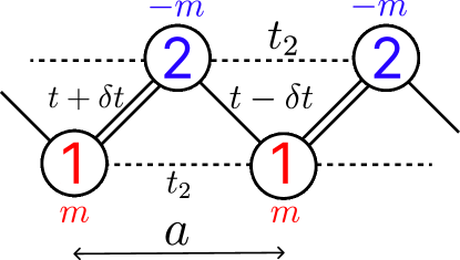
Figure 4: The illustration of the Hamiltonian given by Eq. (97).

We assume spin-singlet microscopic interactions

$$\hat{H}_{\mathrm{int}}=-\sum_{i,l}g_{l}\hat{c}_{x,l\uparrow}^{\dagger}\hat{c}_{x,l\downarrow}^{\dagger}\hat{c}_{x,l\downarrow}\hat{c}_{x,l\uparrow},$$ (98)

where $g_{l}>0$ is the coupling constant, for which we have

$$V^{l_{1}l_{2}l_{3}l_{4}}(x-y)=\frac{1}{2}\delta_{l_{1}l_{2}}\delta_{l_{2}l_{3}}\delta_{l_{3}l_{4}}\delta_{x,y}\,g_{l_{1}}.$$ (99)

We define the Fourier transform

$$\hat{c}_{x,1s}=\frac{1}{\sqrt{N}}\sum_{k}\hat{c}_{k,1s}e^{ikxa},$$ (100)

$$\hat{c}_{x,2s}=\frac{1}{\sqrt{N}}\sum_{k}\hat{c}_{k,2s}e^{ik(x+1/2)a},$$ (101)

where $N$ denotes the number of unit cells and $a$ is the lattice constant. The interaction term can be expressed as

$$\hat{H}_{\mathrm{int}}=-\frac{1}{N}\sum_{k,p,q,l}g_{l}\hat{c}_{k+q,l\uparrow}^{\dagger}\hat{c}_{-k+q,l\downarrow}^{\dagger}\hat{c}_{-p+q,l\downarrow}\hat{c}_{p+q,l\uparrow}$$ (102)

in momentum space. We apply the mean-field approximation in the Cooper channel and define the gap function as

$$\Delta_{l}=-\frac{g_{l}}{N}\sum_{p}\langle\hat{c}_{-p+q,l\downarrow}\hat{c}_{p+q,l\uparrow}\rangle.$$ (103)

Thus, the mean-field Hamiltonian is expressed as

$$\hat{H}_{\mathrm{MF}} =\sum_{k}\hat{\psi}_{k}^{\dagger}\begin{pmatrix}H_{N}(k)&\Delta\\ \Delta&-H_{N}(-k)^{T}\end{pmatrix}\hat{\psi}_{k},$$ (104)

where

$$H_{N}(k) =(t_{2}\cos ka-\mu)\sigma_{0}+t\cos(ka/2)\sigma_{1}$$

$$\qquad-\delta t\sin(ka/2)\sigma_{2}+m\sigma_{3},$$ (105)

and $\Delta=\mathrm{diag}\{\Delta_{1},\Delta_{2}\}$. In this model, previous studies have investigated the linear optical response of collective modes [36] and the linear and second-order optical responses without vertex corrections [7]. For these specific examples, we apply the generalized CFOP method. We investigate the effects of vertex corrections on the nonlinear optical response

Since our derivation of the Ward identity in Secs. II and III was for continuum models, let us check the Ward identity for lattice models using the Rice-Mele model in Eq. (97) as an example. The bare one-photon vertex of this model is given by

$$\gamma(k,q)$$

$$=\frac{a}{2}\tau_{0}\otimes\bigg{[}t_{2}\bigg{(}\sin(ka+\frac{qa}{4})+\sin(ka+\frac{3qa}{4})\bigg{)}\sigma_{0}$$

$$\qquad+t\sin(\frac{ka}{2}+\frac{qa}{4})\sigma_{1}+\delta t\cos(\frac{ka}{2}+\frac{qa}{4})\sigma_{2}\bigg{]},$$ (106)

which satisfies

$$\frac{4}{a}\sin(\frac{qa}{4})\gamma(k,q)+q_{0}\tau_{3}=G_{0}^{-1}(k+q)\tau_{3}-\tau_{3}G_{0}^{-1}(k).$$ (107)

This equation corresponds to the Ward identity (13) for the bare one-photon vertex of continuum models. The Ward identities for the correction parts in Eq. (17) are also satisfied. This is because the proof in the continuum model presented in Eq. (62) remains valid even if the spatial derivative $\partial_{z}$ is replaced by the lattice difference operator.

IV.2.2 Calculations of the full photon vertices based on the CFOP method

Let us introduce the gauge field and consider the electromagnetic responses. Substituting Eq. (99) into Eq. (90), the gap function is given by

$$[\Delta_{A}(x,y)]_{ll^{\prime}}=\delta_{ll^{\prime}}\Delta_{l,A}(x,y),$$ (108)

$$\Delta_{l,A}(x,y)=-V_{l}(x-y)\mathrm{Tr}\big{[}P_{ll}G_{A}(x,y)\big{]},$$ (109)

where $V_{l}(x-y)=g_{l}\delta(\bm{x-y})\delta(x_{0}-y_{0}-0^{-})$. Let us separate the gap function into the real part and the imaginary part as $\Delta_{l,A}(x,y)=\Delta_{1,l,A}(x,y)-i\Delta_{2,l,A}(x,y)$, where each part is determined by the gap equation

$$\Delta_{i,l,A}(x,y)=-\frac{V_{l}(x-y)}{2}\mathrm{Tr}\bigg{[}\tau_{i}\otimes E_{ll}G_{A}(x,y)\bigg{]}.$$ (110)

The self-energy can be rewritten as

$$\Sigma_{A}(x,y)=\sum_{l=1,2}\sum_{i=1,2}\Delta_{i,l,A}(x,y)\tau_{i}\otimes E_{ll}.$$ (111)

By definition [Eq. (16)], the correction part of the full one-photon vertex is given by

$$\Lambda^{\mu}(x,y,w) =-\left.\functionalderivative{\Sigma_{A}(x,y)}{A_{\mu}(w)}\right|_{A=0}$$

$$=-\sum_{i,l}\left.\functionalderivative{\Delta_{i,l,A}(x,y)}{A_{\mu}(w)}\right|_{A=0}\tau_{i}\otimes E_{ll}.$$ (112)

Plugging the gap equation [Eq. (110)] into this, we obtain the following equation that each component should satisfy:

$$-\left.\functionalderivative{\Delta_{i,l,A}(x,y)}{A_{\mu}(w)}\right|_{A=0}$$

$$=\frac{V_{l}(x-y)}{2}\left.\functionalderivative{A_{\mu}(w)}\mathrm{Tr}\big{[}\tau_{i}\otimes E_{ll}G_{A}(x,y)\big{]}\right|_{A=0}$$

$$=-\frac{V_{l}(x-y)}{2}\mathrm{Tr}\big{[}\tau_{i}\otimes E_{ll}G(x,\overline{x}^{\prime})$$

$$\qquad\times\big{(}\gamma^{\mu}(\overline{x}^{\prime},\overline{y}^{\prime},w)+\Lambda^{\mu}(\overline{x}^{\prime},\overline{y}^{\prime},w)\big{)}G(\overline{y}^{\prime},y)\big{]}.$$ (113)

This is the integral equation of the correction parts $\Lambda^{\mu}$. This can be solved if we assume a solution of the form

$$-\left.\functionalderivative{\Delta_{i,l,A}(x,y)}{A_{\mu}(w)}\right|_{A=0}=\Lambda_{il}^{\mu}(x,w)\delta(x-y).$$ (114)

Performing the Fourier transform, the integral equation reduces to the easily solvable matrix equation

$$\sum_{j,l^{\prime}}\bigg{(}\frac{2}{g_{l}}\delta_{il,jl^{\prime}}-Q_{il,jl^{\prime}}(q)\bigg{)}\Lambda_{jl^{\prime}}^{\mu}(q)=Q_{il}^{\mu}(q),$$ (115)

where

$$Q_{il}^{\mu}(q)=-\mathrm{Tr}\big{[}\tau_{i}\otimes E_{ll}G(\overline{p}+q)\gamma^{\mu}(p,q)G(\overline{p})\big{]},$$ (116)

$$Q_{il,jl^{\prime}}(q)=-\mathrm{Tr}\big{[}\tau_{i}\otimes E_{ll}G(\overline{p}+q)\tau_{j}\otimes E_{l^{\prime}l^{\prime}}G(\overline{p})\big{]}$$ (117)

are correlation functions related to fluctuations of order parameters. By solving this, we can obtain the gauge-invariant electromagnetic responses. The optical responses can be obtained by the limit $\bm{q}\to 0$.

Similarly, the correction part of the full two-photon vertex can be obtained by calculating

$$\Lambda^{\mu\nu}(x,y,w_{1},w_{2})=\sum_{i,l}\frac{\delta^{2}\Delta_{i,l,A}(x,y)}{\delta A_{\mu}(w_{1})\delta A_{\nu}(w_{2})}\tau_{i}\otimes E_{ll}.$$ (118)

Detailed calculations are discussed in Appendix C.

Let us make a comment on the relation between our work and the previous studies of the collective mode in superconductors [36, 37, 38]. The vertex corrections in our formulation turn out to be equivalent to the random phase approximation (RPA) at the linear response level. To see this, note that the matrix equation (115) for $\Lambda^{\mu}$ can be rewritten as

$$(1+U\Pi)\vec{\Lambda}^{\mu}=U\vec{Q}^{\mu},$$ (119)

where $U=\mathrm{diag}\{g_{1},g_{2},g_{1},g_{2}\}$ is the interaction matrix,

$$[\Pi]_{il,jl^{\prime}}=-\frac{1}{2}Q_{il,jl^{\prime}}(q)$$ (120)

is the matrix corresponding to the bubble diagram, $\vec{\Lambda^{\mu}}=(\Lambda_{11}^{\mu},\Lambda_{12}^{\mu},\Lambda_{21}^{\mu},\Lambda_{22}^{\mu})^{T}$ and $\vec{Q}^{\mu}=(Q_{11}^{\mu},Q_{12}^{\mu},Q_{21}^{\mu},Q_{22}^{\mu})^{T}/2$. Since the effective interaction within the RPA [Fig. 5] is given by

$$U_{\mathrm{eff}}=\frac{U}{1+U\Pi},$$ (121)

the correction parts of the full one-photon vertices are

$$\vec{\Lambda}^{\mu}=U_{\mathrm{eff}}\vec{Q}^{\mu}.$$ (122)

Therefore, the generalized CFOP method is equivalent to the RPA in this case. A significant advantage of our framework is that it easily extends to nonlinear responses and clearly demonstrates their gauge invariance. Our approach emphasizes the perspective that collective excitations in superconductors restore the gauge invariance.

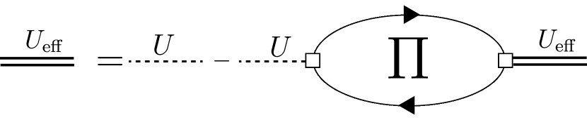
Figure 5: The diagrammatic representation of the effective interaction $U_{\mathrm{eff}}$ within RPA.

IV.2.3 Collective mode excitations

First, let us see responses of collective mode. In multi-band superconductors, there can occur a collective excitation known as the Leggett mode, corresponding to the fluctuations of the phase difference between the two order parameters [40]. Here, we calculate the linear and second-order optical responses based on the generalized CFOP method.

We set the parameters as $t=0.2$, $\mu=-0.3$, $\delta t=0.1$, $m=0.3$, $t_{2}=1.0$, $\Delta_{1}=0.2$, $\Delta_{2}=0.175$, $\eta=1\times 10^{-2}$, and $a=1$ so that our calculation reproduce the result of the previous study [36]. Instead of solving the gap equation with given coupling constant $g_{l}$, we set the magnitude of the gap $\Delta_{l}$ and determined the corresponding coupling constant $g_{l}$ through numerical calculations, yielding $g_{1}=g_{2}\simeq 0.990$.

Figure 6: The linear and second-order optical responses with vertex corrections in multi-band superconductors. (a) The band structure. (b) The real part of the linear optical conductivity $\sigma^{xx}(\omega)$. The blue corresponds to the calculation without vertex corrections, and the orange corresponds to the calculation with vertex corrections. (c) The real part of the second harmonic generation $\sigma^{xxx}(\omega,\omega)$. (d) The real part of the photocurrent generation $\sigma^{xxx}(\omega,-\omega)$.

The band dispersion of the BdG Hamiltonian under this parameter setting is shown in Fig. 6(a), and the calculated linear optical response is presented in Fig. 6(b). It is evident that while the quasiparticle excitation peak around $\omega\simeq 0.7$ remains nearly unchanged, a new excitation peak emerges near $\omega\simeq 0.2$. This newly observed excitation peak corresponds to the Leggett mode, successfully reproducing the result of the previous study [36].

While previous study [36] focused solely on linear responses, the generalized CFOP method allows for the straightforward calculation of nonlinear responses with vertex corrections. The results of the second-order optical response are shown in Fig. 6(d) and Fig. 6(e). Similar to the linear optical response, sharp new excitation peaks emerge around $\omega\simeq 0.2$ and $2\omega\simeq 0.2$.

IV.2.4 The suppression of the nonlinear optical conductivity

Next, let us consider the situation addressed in Ref. [7]. It discusses systems with spatial inversion symmetry in the normal conducting phase, where the superconducting gap breaks this symmetry, resulting in linear and second-order optical responses. However, its calculation does not include many-body effects and lacks gauge-invariant treatment. We demonstrate differences that arise when employing the generalized CFOP method.

We set the parameters as $t=1$, $\mu=0.8$, $\delta t=0.5$, $m=0$, $t_{2}=0$, $\Delta_{1}=0.2$, $\Delta_{2}=0.1$, $\eta=1\times 10^{-3}$, and $a=2$ so that bare calculations reproduce the result of the previous study [7].

Figure 7: The linear and second-order optical responses with vertex corrections in multi-band superconductors. (a) The band structure. (b) The real part of the linear optical conductivity $\sigma^{xx}(\omega)$. The blue corresponds to the calculation without vertex corrections, and the orange corresponds to the calculation with vertex corrections. (c) The real part of the linear optical conductivity with a focus on low-energy excitations around the superconducting gap. (d) The real part of the second harmonic generation $\sigma^{xxx}(\omega,\omega)$. (e) The real part of the photocurrent generation $\sigma^{xxx}(\omega,-\omega)$.

The calculated linear optical response is presented in Fig. 7(c). Even in this case, it is evident that the new excitation peak emerges near $\omega\simeq 1.3$ due to the vertex corrections. The previous study [7] focused on low-energy quasiparticle excitations near the superconducting gap. Therefore, we examine the effect of vertex corrections at this energy scale. Fig. 7(d) presents the calculation results of the linear optical response in the low-energy region, while Fig.7(e) and Fig.7(f) show the second-order optical responses. The calculations without vertex corrections successfully reproduce the result from the previous study. It is apparent that vertex corrections significantly alter the results without vertex corrections. The linear optical response in the low-energy region is strongly suppressed and almost completely disappears. The vertex corrections also suppress the magnitude of second-order optical conductivity $\sigma^{xxx}(\omega_{1},\omega_{2})$ and may change the sign of it.

IV.3 Optical responses in $d$-wave superconductors

IV.3.1 Model

Our formulation can be applied to the anisotropic pairing. As an example, let us consider spin-singlet $d$-wave superconductors on a square lattice. The normal-state Hamiltonian is defined by

$$\hat{H}_{N}=\sum_{\bm{k}s}\hat{c}_{\bm{k}s}^{\dagger}\epsilon(\bm{k})\hat{c}_{\bm{k}s}$$ (123)

where $\epsilon(\bm{k})=t(2-\cos k_{x}-\cos k_{y})-\mu$. The microscopic interaction in real space is given by

$$V^{s_{1}s_{2}s_{3}s_{4}}(\bm{x-y})=\frac{1}{2}V(\bm{x-y})(i\sigma_{2})_{s_{1}s_{2}}(i\sigma_{2})_{s_{3}s_{4}}^{\dagger},$$ (124)

where $V(\bm{x-y})=g\sum_{\mu=x,y}(\delta_{\bm{x,y+e_{\mu}}}+\delta_{\bm{x,y-e_{\mu}}})$. In momentum space, this interaction can be expressed as

$$\hat{H}_{\mathrm{int}}=-\frac{g}{N}\sum_{\bm{k,p,q}}\phi_{d}(\bm{k})\phi_{d}(\bm{p})\hat{c}_{\bm{k+q}\uparrow}^{\dagger}\hat{c}_{\bm{-k+q}\downarrow}^{\dagger}\hat{c}_{\bm{-p+q}\downarrow}\hat{c}_{\bm{p+q}\uparrow},$$ (125)

where $\phi_{d}(\bm{k})=\cos k_{x}-\cos k_{y}$ is the $d$-wave form factor. Employing the mean-field approximation in the Cooper channel, one defines the magnitude of the gap as

$$\Delta_{d}=-\frac{g}{N}\sum_{\bm{p}}\langle\hat{c}_{-\bm{p}\downarrow}\hat{c}_{\bm{p}\uparrow}\rangle\phi_{d}(\bm{p}),$$ (126)

the interaction term reduces to

$$\hat{H}_{\mathrm{int}}\to\sum_{\bm{k}}(\Delta_{d}\phi_{d}(\bm{k})\hat{c}_{\bm{k}\uparrow}^{\dagger}\hat{c}_{\bm{-k}\downarrow}^{\dagger}+h.c.)$$ (127)

which describes $d$-wave pairing in the superconducting state.

Since the optical transitions between the particle-hole pairs are prohibited in the presence of time-reversal symmetry and spatial inversion symmetry [41], we consider the situation where Cooper pairs have finite momentum and break inversion symmetry. In this case, as already presented in Sec. III.3, the magnitude of the gap is defined as

$$\Delta_{d}=-\frac{g}{N}\sum_{\bm{p}}\phi_{d}(\bm{p})\langle\hat{c}_{\bm{-p+Q}\downarrow}\hat{c}_{\bm{p+Q}\uparrow}\rangle,$$ (128)

where $\bm{2}Q$ is the momentum of the Cooper pairs. The mean-field Hamiltonian is given by

$$\hat{H}_{MF}=\sum_{\bm{k}}(\hat{\psi}_{\bm{k}}^{\bm{Q}})^{\dagger}\begin{pmatrix}\epsilon(\bm{k+Q})&\Delta_{d}\phi_{d}(\bm{k})\\ \Delta_{d}\phi_{d}(\bm{k})&-\epsilon(\bm{k-Q})\end{pmatrix}\hat{\psi}_{\bm{k}}^{\bm{Q}}.$$ (129)

The previous study [28] investigated the optical responses in this model with vertex corrections, although its theoretical treatment is different. In the subsequent sections, we compare the generalized CFOP method with that of the previous work [28].

IV.3.2 The full photon vertices

Now, let us calculate the full vertices based on the generalized CFOP method. The microscopic interaction in Eq. (124) leads to the the self-energy of superconductors [Eqs. (89) and (90)]:

$$\Sigma_{A}(x,y)=\begin{pmatrix}&\Delta_{A}(x,y)\\ \Delta_{A}^{\dagger}(x,y)&\end{pmatrix},$$ (130)

$$\Delta_{A}(x,y)=-V(x-y)\mathrm{Tr}\big{[}PG_{A}(x,y)\big{]},$$ (131)

where $V(x-y)=V(\bm{x-y})\delta(x_{0}-y_{0}-0^{-})$. If we separate the real part and imaginary part of the gap function as $\Delta_{A}(x,y)=\Delta_{1,A}(x,y)-i\Delta_{2,A}(x,y)$, each part satisfies

$$\Delta_{i,A}(x,y)=-\frac{1}{2}V(x-y)\mathrm{Tr}\big{[}\tau_{i}G_{A}(x,y)\big{]},$$ (132)

and the self-energy can be expressed as

$$\Sigma_{A}(x,y)=\Delta_{1,A}(x,y)\tau_{1}+\Delta_{2,A}(x,y)\tau_{2}.$$ (133)

The correction part $\Lambda^{\mu}$ of the full one-photon vertex is given by the functional derivatives of the self-energy as in Eq. (16):

$$\Lambda^{\mu}(x,y,z)=\sum_{i=1,2}\Lambda_{i}^{\mu}(x,y,z)\tau_{i},$$ (134)

where

$$\Lambda_{i}^{\mu}(x,y,z)=-\left.\functionalderivative{\Delta_{i,A}(x,y)}{A_{\mu}(z)}\right|_{A=0}.$$ (135)

The functional derivative of the gap equation in Eq. (132) and the Fourier transform lead to

$$\Lambda_{i}^{\mu}(k,q) =-V(k-p)\mathrm{Tr}\bigg{[}\tau_{i}G(\overline{p}+q)$$

$$\times\bigg{(}\gamma^{\mu}(\overline{p},q)+\sum_{j=1}^{2}\tau_{j}\Lambda_{j}^{\mu}(\overline{p},q)\bigg{)}G(\overline{p})\bigg{]},$$ (136)

where $V(k-p)$ is the Fourier transform of $V(x-y)$.

To solve this integral equation, let us expand $V(k-p)$ as

$$V(k-p)=2g\sum_{n=1}^{4}f_{n}(\bm{k})f_{n}(\bm{p}),$$ (137)

where we defined $f_{1}(\bm{k})=\cos k_{x},f_{2}(\bm{k})=\cos k_{y},f_{3}(\bm{k})=\sin k_{x},f_{4}(\bm{k})=\sin k_{y}.$ Similarly, we expand the solution to the integral equation as

$$\Lambda_{i}^{\mu}(k,q) =\sum_{n=1}^{4}f_{n}(\bm{k})\Lambda_{in}^{\mu}(q).$$ (138)

If each component $\Lambda_{i,n}^{\mu}(q)$ satisfies

$$\Lambda_{in}^{\mu}(q) =-gf_{n}(\overline{\bm{p}})\mathrm{Tr}\big{[}\tau_{i}G(\overline{p}+q)$$

$$\times\big{(}\gamma^{\mu}(\overline{p},q)+\sum_{j,m}\tau_{j}f_{m}(\overline{p})\big{)}G(\overline{p})\big{]}\Lambda_{jm}^{\mu}(q),$$ (139)

it will be the solution to Eq. (136). Therefore, we need to solve the matrix equation given by

$$\sum_{j,m}\bigg{(}\frac{1}{g}\delta_{in,jm}-Q_{in,jm}(q)\bigg{)}\Lambda_{jm}^{\mu}(q)=Q_{in}^{\mu}(q),$$ (140)

where

$$Q_{in,jm}(q)=-f_{n}(\overline{p})f_{m}(\overline{p})\mathrm{Tr}\bigg{[}\sigma_{i}G(\overline{p}+q)\sigma_{j}G(\overline{p})\bigg{]},$$ (141)

$$Q_{in}^{\mu}(q)=-f_{n}(\overline{p})\mathrm{Tr}\bigg{[}\sigma_{i}G(\overline{p}+q)\gamma^{\mu}(\overline{p},q)G(\overline{p})\bigg{]}.$$ (142)

Before proceeding to numerical calculations, let us review the construction of the full photon vertex in the previous study [28]. In the previous study, the Fock approximation of the self-energy

$$\Sigma(k)=V(\bm{k,\overline{p}})\tau_{3}G(\overline{p})\tau_{3}$$ (143)

is employed and the full photon vertex is given as the solution to the Bethe-Salpeter equation

$$\Gamma^{\nu}(k,q)=\gamma^{\nu}(k,q)+V(\bm{k,\overline{p}})\tau_{3}G(\overline{p}+q)\Gamma^{\nu}(\overline{p},q)G(\overline{p})\tau_{3}$$ (144)

where $V(\bm{k,p})=\phi_{d}(\bm{k})\phi_{d}(\bm{p})$. However, this approach does not necessarily satisfy the Ward identity strictly. When checking the Ward identity for the correction part [Eq. (17)], one obtains

$$\Lambda^{\nu}(k,q)q_{\nu}$$

$$=V(\bm{k,\overline{p}})\tau_{3}G(\overline{p}+q)\Gamma^{\nu}(\overline{p},q)q_{\nu}G(\overline{p})\tau_{3}$$

$$=V(\bm{k,\overline{p}})\tau_{3}G(\overline{p}+q)$$

$$\qquad\times\big{(}G^{-1}(\overline{p}+q)\tau_{3}-\tau_{3}G^{-1}(\overline{p})\big{)}G(\overline{p})\tau_{3}$$

$$=V(\bm{k,\overline{p}})G(\overline{p})\tau_{3}-V(\bm{k,\overline{p}})\tau_{3}G(\overline{p}+q)$$

$$=\tau_{3}\Sigma(k)-V(\bm{k,\overline{p}})\tau_{3}G(\overline{p}+q),$$ (145)

which deviates from the expected form.

Therefore, in such a formulation, gauge-invariant responses might not be obtained. In the generalized CFOP method, such issues do not arise, and we can obtain full photon vertices that manifestly satisfy the Ward identities.

We compare the correction parts obtained by two different methods. The correction part derived by the generalized CFOP method is given by Eqs. (134) and (138). In the case of the Bethe-Salpeter equation, the correction part of the full one-photon vertex is expanded in the Pauli basis as

$$\Lambda^{\mu}(k,q)=\sum_{i=0}^{3}\Lambda_{i}^{\mu}(k,q)\tau_{i},$$ (146)

and the $k$-dependence is assumed to be

$$\Lambda_{i}^{\mu}(k,q)=\phi_{d}(\bm{k})\Lambda_{i}^{\mu}(q).$$ (147)

These two methods for constructing the full vertex differ in whether the $\tau_{0},\tau_{3}$ components are present in the correction part. This difference stems from the form of the self-energies in Eqs. (133) and (143). The $k$-dependence of $\Lambda_{i}^{\mu}(k,q)$ is also different. The solutions to the Bethe-Salpeter equation always respect $d$-wave symmetry $\phi_{d}(\bm{k})$, whereas the solutions to Eq. (136) do not. We will demonstrate these differences using numerical calculations in the next section.

IV.3.3 Numerical calculations

We conduct numerical calculations to investigate how the results based on the generalized CFOP method are different from the results of the previous study [28]. We introduce the momentum of the Cooper pairs along $x$-direction $\bm{Q}=Q_{x}\bm{e_{x}}$ and set the parameters as $t=1.0\times 10^{2}$, $\mu=9.0\times 10^{1}$, $\Delta_{d}=2.3\times 10^{1}$, $\eta=3\times 10^{-2}$, $Q_{x}=0.07$, yielding the coupling constant $g\simeq 1.8\times 10^{2}$ so that we reproduce the result of the previous study [28]. The numerical results for the optical responses are summarized in Fig. 8.

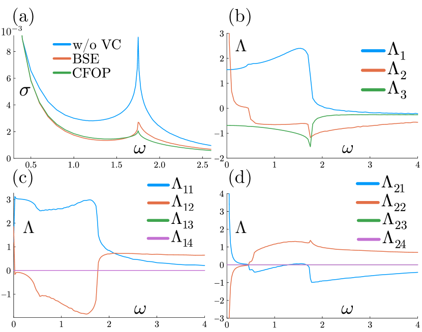
Figure 8: (a) The real part of optical conductivity $\sigma^{xx}(\omega)$ with and without vertex corrections. The blue refers to the calculation without vertex corrections, the orange corresponds to the calculation with vertex corrections based on the Bethe-Salpeter equation, and the green corresponds to the calculation based on the full vertex derived in this study. (b) The real part of the solution $\Gamma_{i}^{x}(\omega)$ to the Bethe-Salpeter equation. The $\sigma_{0}$ component $\Lambda_{0}^{\mu}$ is not shown because it is always zero. (c) The real part of $\Gamma_{1n}^{x}(\omega)$. (d) The real part of $\Gamma_{2n}^{x}(\omega)$.

We compare the optical conductivity with different methods in Fig. 8(a). It reveals that the optical responses computed using the generalized CFOP method exhibit slight quantitative differences compared to those based on the Bethe-Salpeter equation.

Since the differences in the optical responses are minor, let us focus on the correction part of the full one-photon vertex. First, we see the each Pauli component $\Lambda_{i}^{\mu}$. The correction part based on the generalized CFOP method consists of the off-diagonal components $\tau_{1}$,$\tau_{2}$. On the other hand, the numerical calculation reveals that the solution of the Bethe-Salpeter equation contains the three finite Pauli components: $\tau_{1}$, $\tau_{2}$, and $\tau_{3}$. The $\tau_{0}$ component is found to be analytically zero.

Next, we investigate the $k$-dependence of the correction part $\Lambda^{\mu}(k,q)$. While the solution of the Bethe-Salpeter equation always respects the $d$-wave symmetry as expressed in Eq. (147), the correction parts obtained by the generalized CFOP method do not necessarily. The $d$-wave symmetry is realized when the conditions

$$\Lambda_{i1}^{\mu}(q) =-\Lambda_{i2}^{\mu}(q),$$ (148)

$$\Lambda_{i3}^{\mu}(q) =\Lambda_{i4}^{\mu}(q)=0$$ (149)

hold. As shown in Fig. 8(c),(d), these conditions are clearly not satisfied. Thus, the numerical results indicate that the correction parts do not exhibit $d$-wave symmetry. This reflects the fact that the acquisition of momentum in the $x$-direction by the Cooper pairs breaks $C_{4}$ rotational symmetry.

V Conclusion

In this paper, we discussed the gauge-invariant formulation of electromagnetic response in superconductors. We summarized the Feynman rules for the electromagnetic response kernel in interacting systems and proved its gauge invariance using the Ward identity. We developed a systematic formulation of the full photon vertices that manifestly satisfy the Ward identities. Using this framework, we numerically investigated the impact of vertex corrections on optical responses. The resulting behavior exhibits significant qualitative and quantitative changes. For unconventional superconductors, our full photon vertex differs from existing studies. We thus conclude that it is crucial to treat optical responses in superconductors in a gauge-invariant manner.

In this study, we assumed that the interactions among electrons in the microscopic Hamiltonian are not affected by the gauge field. As a result, pair-hopping interactions, for example, cannot be treated in our present formulation. Extension to such cases is left as a future work.

Appendix A The detailed derivation of the Ward identities

In this appendix, we present the detailed derivation of the Ward identities. Given a classical gauge field $A_{\mu}$, the generating functional for correlation functions is defined by

$$Z[A_{\mu},\bar{\eta},\eta]=\int\mathcal{D}\bar{\psi}\mathcal{D}\psi\exp[-S[A_{\mu},\bar{\psi},\psi]+\int d^{4}x(\bar{\eta}(x)\psi(x)+\bar{\psi}(x)\eta(x))],$$ (150)

where $\bar{\eta},\eta$ are sources and $S[A_{\mu},\bar{\psi},\psi]$ is the action of electronic system. Furthermore, assuming that the action $S[A_{\mu},\bar{\psi},\psi]$ is invariant under local $U(1)$ gauge transformation

$$A_{\mu}\to A_{\mu}-\partial_{\mu}\theta,\bar{\psi}\to\bar{\psi}e^{-i\theta\tau_{3}},\psi\to e^{i\theta\tau_{3}}\psi,$$ (151)

we have

$$S[A_{\mu}-\partial_{\mu}\theta,\bar{\psi}e^{-i\theta\tau_{3}},e^{i\theta\tau_{3}}\psi]=S[A_{\mu},\bar{\psi},\psi].$$ (152)

We also define the functional

$$W[A_{\mu},\bar{\eta},\eta]=-\ln Z[A_{\mu},\bar{\eta},\eta],$$ (153)

and the effective action

$$\Gamma[A_{\mu},\bar{\phi},\phi]=W[A_{\mu},\bar{\eta},\eta]+\int d^{4}x(\bar{\eta}(x)\phi(x)+\bar{\phi}(x)\eta(x)).$$ (154)

by the Legendre transformation of the functional $W[A_{\mu},\bar{\eta},\eta]$, where

$$\functionalderivative{W[A_{\mu},\bar{\eta},\eta]}{\bar{\eta}(x)}=-\phi(x),\quad\functionalderivative{W[A_{\mu},\bar{\eta},\eta]}{\eta(x)}=\bar{\phi}(x).$$ (155)

Relying on the general properties of the Legendre transformation, we obtain the inverse transformation

$$\functionalderivative{\Gamma[A_{\mu},\bar{\phi},\phi]}{\phi(x)}=-\bar{\eta}(x),\quad\functionalderivative{\Gamma[A_{\mu},\bar{\phi},\phi]}{\bar{\phi}(x)}=\eta(x).$$ (156)

From the local $U(1)$ symmetry of the action $S[A_{\mu},\bar{\psi},\psi]$, we can also demonstrate the local $U(1)$ invariance of $Z[A_{\mu},\bar{\eta},\eta]$ and $W[A_{\mu},\bar{\eta},\eta]$. If we perform the local $U(1)$ transformation on the gauge field and sources as

$$A_{\mu}^{\prime}=A_{\mu}-\partial_{\mu}\theta,\quad\bar{\eta}^{\prime}=\bar{\eta}e^{-i\theta\tau_{3}},\quad\eta^{\prime}=e^{i\theta\tau_{3}}\eta,$$ (157)

the generating functional is modified to

$$Z[A_{\mu}^{\prime},\bar{\eta}^{\prime},\eta^{\prime}]=\int\mathcal{D}\bar{\psi}\mathcal{D}\psi\exp[-S[A_{\mu}-\partial_{\mu}\theta,\bar{\psi},\psi]+\int d^{4}x\left(\bar{\eta}e^{-i\theta\tau_{3}}\psi+\bar{\psi}e^{i\theta\tau_{3}}\eta\right)].$$ (158)

Transforming the fields integrated in the functional integral as

$$\bar{\psi}^{\prime}=\bar{\psi}e^{i\theta\tau_{3}},\quad\psi^{\prime}=e^{-i\theta\tau_{3}}\psi,$$ (159)

we obtain the local $U(1)$ symmetry of the generating functional

$$Z[A_{\mu}^{\prime},\bar{\eta}^{\prime},\eta^{\prime}] =\int\mathcal{D}\bar{\psi^{\prime}}\mathcal{D}\psi^{\prime}\exp[-S[A_{\mu}-\partial_{\mu}\theta,\bar{\psi}^{\prime}e^{-i\theta\tau_{3}},e^{i\theta\tau_{3}}\psi^{\prime}]+\int d^{4}x\left(\bar{\eta}\psi^{\prime}+\bar{\psi}^{\prime}\eta\right)]$$

$$=\int\mathcal{D}\bar{\psi^{\prime}}\mathcal{D}\psi^{\prime}\exp[-S[A_{\mu},\bar{\psi^{\prime}},\psi^{\prime}]+\int d^{4}x\left(\bar{\eta}\psi^{\prime}+\bar{\psi^{\prime}}\eta\right)]$$

$$=Z[A_{\mu},\bar{\eta},\eta].$$ (160)

As a result, $W[A_{\mu},\bar{\eta},\eta]$ is also invariant under the local $U(1)$ transformation.

Due to the invariance under local $U(1)$ transformation, we obtain

$$\int d^{4}z\left[-\functionalderivative{W[A_{\mu},\bar{\eta},\eta]}{A_{\mu}(z)}\partial_{z^{\mu}}\theta(z)-i\bar{\eta}(z)\tau_{3}\functionalderivative{W[A_{\mu},\bar{\eta},\eta]}{\bar{\eta}(z)}\theta(z)-i\functionalderivative{W[A_{\mu},\bar{\eta},\eta]}{\eta(z)}\tau_{3}\eta(z)\theta(z)\right]=0.$$ (161)

Since this equation holds for any function $\theta$,

$$\partial_{z^{\mu}}\functionalderivative{W[A_{\mu},\bar{\eta},\eta]}{A_{\mu}(z)}=i\left(\bar{\eta}(z)\tau_{3}\functionalderivative{W[A_{\mu},\bar{\eta},\eta]}{\bar{\eta}(z)}+\functionalderivative{W[A_{\mu},\bar{\eta},\eta]}{\eta(z)}\tau_{3}\eta(z)\right)$$ (162)

must hold. Rewriting this using the effective action $\Gamma[A_{\mu},\bar{\phi},\phi]$, we get

$$\partial_{z^{\mu}}\functionalderivative{\Gamma[A_{\mu},\bar{\phi},\phi]}{A_{\mu}(z)}=i\left(\functionalderivative{\Gamma[A_{\mu},\bar{\phi},\phi]}{\phi(z)}\tau_{3}\phi(z)+\bar{\phi}(z)\tau_{3}\functionalderivative{\Gamma[A_{\mu},\bar{\phi},\phi]}{\bar{\phi}(z)}\right).$$ (163)

By further performing functional derivatives of this equation, we can derive the Ward identities of the desired order. First, differentiating with respect to $\phi(y)$ and setting $\phi=0$, we get

$$\partial_{z^{\mu}}\left.\frac{\delta^{2}\Gamma[A_{\mu},\bar{\phi},\phi]}{\delta A_{\mu}(z)\delta\phi(y)}\right|_{\phi=0}=i\left(\bar{\phi}(z)\tau_{3}\left.\frac{\delta^{2}\Gamma[A_{\mu},\bar{\phi},\phi]}{\delta\bar{\phi}(z)\delta\phi(y)}\right|_{\phi=0}-\left.\functionalderivative{\Gamma[A_{\mu},\bar{\phi},\phi]}{\phi(z)}\right|_{\phi=0}\tau_{3}\delta(y-z)\right).$$ (164)

Furthermore, differentiating with respect to $\bar{\phi}(x)$ and $\bar{\phi}=0$, we get

$$\partial_{z^{\mu}}\left.\frac{\delta^{3}\Gamma[A_{\mu},\bar{\phi},\phi]}{\delta A_{\mu}(z)\delta\bar{\phi}(x)\delta\phi(y)}\right|_{\bar{\phi}=\phi=0} =i\left(\delta(x-z)\tau_{3}\left.\frac{\delta^{2}\Gamma[A_{\mu},\bar{\phi},\phi]}{\delta\bar{\phi}(z)\delta\phi(y)}\right|_{\bar{\phi}=\phi=0}-\left.\frac{\delta^{2}\Gamma[A_{\mu},\bar{\phi},\phi]}{\delta\bar{\phi}(x)\phi(z)}\right|_{\bar{\phi}=\phi=0}\tau_{3}\delta(y-z)\right).$$ (165)

The functional derivatives of the effective action are related to the inverse of the Green function. This can be shown by the equation

$$\tau_{0}\delta(x-y)=\functionalderivative{\bar{\eta}(y)}{\bar{\eta}(x)}=\int d^{4}z\functionalderivative{\bar{\phi}(z)}{\bar{\eta}(x)}\functionalderivative{\bar{\eta}(y)}{\bar{\phi}(z)}=\int d^{4}z\frac{\delta^{2}W[A_{\mu},\bar{\eta},\eta]}{\delta\bar{\eta}(x)\delta\eta(z)}\left(-\frac{\delta^{2}\Gamma[A_{\mu},\bar{\phi},\phi]}{\delta\bar{\phi}(z)\delta\phi(y)}\right).$$ (166)

By setting, $\bar{\eta}=\eta=\bar{\phi}=\phi=0$, we obtain

$$\left.\frac{\delta^{2}\Gamma[A_{\mu},\bar{\phi},\phi]}{\delta\bar{\phi}(z)\delta\phi(y)}\right|_{\bar{\phi}=\phi=0}=G_{A}^{-1}(z,y),$$ (167)

where

$$G_{A}(x,y)=-\frac{1}{Z_{A}}\int\mathcal{D}\bar{\psi}\mathcal{D}\psi\psi(x)\bar{\psi}(y)\exp[-S[A_{\mu},\bar{\psi},\psi]]=-\left.\frac{\delta^{2}W[A_{\mu},\bar{\eta},\eta]}{\delta\bar{\eta}(x)\delta\eta(y)}\right|_{\bar{\eta}=\eta=0}$$ (168)

is the full (two-fermion) Green function of the fermion system with the gauge field. Plugging this relation to Eq. (165), we obtain

$$\partial_{z^{\mu}}\functionalderivative{G_{A}^{-1}(x,y)}{A_{\mu}(z)}=i\bigg{(}\delta(x-z)\tau_{3}G_{A}^{-1}(x,y)-G_{A}^{-1}(x,y)\tau_{3}\delta(y-z)\bigg{)}.$$ (169)

From this equation, we can derive the relations that must be satisfied by $n$-photon vertices.

For example, by setting $A=0$ in Eq. (169), we obtain

$$\partial_{z^{\mu}}\Gamma^{\mu}(x,y,z)=i\bigg{(}\delta(x-z)\tau_{3}G^{-1}(x,y)-G^{-1}(x,y)\tau_{3}\delta(y-z)\bigg{)},$$ (170)

where

$$\Gamma^{\mu}(x,y,z)=\left.\frac{\delta^{3}\Gamma[A_{\mu},\bar{\phi},\phi]}{\delta A_{\mu}(z)\delta\bar{\phi}(x)\delta\phi(y)}\right|_{A=\bar{\phi}=\phi=0}=\left.\functionalderivative{G_{A}^{-1}(x,y)}{A_{\mu}(z)}\right|_{A=0}$$ (171)

is the one-photon (two-fermion) vertex and $G$ is the full Green function of the system without the gauge field. This equation is the well-known Ward identity for the one-photon vertex. In the momentum space, the Ward identity for the full one-photon vertex is given by

$$\Gamma^{\mu}(k,q)q_{\mu}=G^{-1}(k+q)\tau_{3}-\tau_{3}G^{-1}(k).$$ (172)

Furthermore, by functionally differentiating Eq. (169) with respect to $A_{\nu}(w)$ and setting $A=0$, we obtain

$$\partial_{z^{\mu}}\left.\frac{\delta^{2}G_{A}^{-1}(x,y)}{\delta A_{\nu}(w)\delta A_{\mu}(z)}\right|_{A=0}=i\left(\delta(x-z)\tau_{3}\left.\functionalderivative{G_{A}^{-1}(x,y)}{A_{\nu}(w)}\right|_{A=0}-\left.\functionalderivative{G_{A}^{-1}(x,y)}{A_{\nu}(w)}\right|_{A=0}\tau_{3}\delta(y-z)\right).$$ (173)

Defining the two-photon vertex as

$$\Gamma^{\nu\mu}(x,y,w,z)=-\left.\frac{\delta^{2}G_{A}^{-1}(x,y)}{\delta A_{\nu}(w)\delta A_{\mu}(z)}\right|_{A=0},$$ (174)

we obtain the Ward identity for the two-photon vertex:

$$\partial_{z^{\mu}}\Gamma^{\nu\mu}(x,y,w,z)=i\left(\Gamma^{\nu}(x,y,w)\tau_{3}\delta(y-z)-\delta(x-z)\tau_{3}\Gamma^{\nu}(x,y,w)\right).$$ (175)

The Ward identities for full multi-photon vertices can be obtained in the same way. By defining the $n$-photon vertex as

$$\Gamma^{\alpha_{1}\cdots\alpha_{n}}(x,y,w_{1},\cdots,w_{n})=(-1)^{n-1}\left.\left(\prod_{i=1}^{n}\functionalderivative{A_{\alpha_{i}}(w_{i})}\right)G_{A}^{-1}(x,y)\right|_{A=0},$$ (176)

the Ward identity for the $n$-photon vertex is given by

$$\partial_{w_{n}^{\alpha_{n}}}\Gamma^{\alpha_{1}\cdots\alpha_{n}}(x,y,w_{1},\cdots,w_{n}) =i\Gamma^{\alpha_{1}\cdots\alpha_{n-1}}(x,y,w_{1},\cdots,w_{n-1})\tau_{3}\delta(y-w_{n})$$

$$\qquad\qquad-i\delta(x-w_{n})\tau_{3}\Gamma^{\alpha_{1}\cdots\alpha_{n-1}}(x,y,w_{1},\cdots,w_{n-1}).$$ (177)

When expressed in the momentum space, it becomes

$$(q_{n})_{\alpha_{n}}\Gamma^{\alpha_{1}\cdots\alpha_{n}}(k,q_{1},\cdots,q_{n}) =\tau_{3}\Gamma^{\alpha_{1}\cdots\alpha_{n-1}}(k,q_{1},\cdots,q_{n-1})$$

$$\qquad-\Gamma^{\alpha_{1}\cdots\alpha_{n-1}}(k+q_{n},q_{1},\cdots,q_{n})\tau_{3}.$$ (178)

Appendix B The diagrammatical method of the full photon vertices of superconductors

In this appendix, we employ the Fock approximation to the self-energy instead of the generalized CFOP method and discuss the gauge-invariant treatment of the electromagnetic responses in this case. The Fock approximation is given by

$$\Sigma_{A}(x,y)=V(x-y)\tau_{3}G_{A}(x,y)\tau_{3}.$$ (179)

First, we show that the Fock approximation is compatible with the Ward identities. We have to check the satisfaction of Eq. (60). This can be shown by

$$\partial_{z^{\mu}}\functionalderivative{\Sigma_{A}(x,y)}{A_{\mu}(z)} =V(x-y)\tau_{3}\partial_{z^{\mu}}\functionalderivative{G_{A}(x,y)}{A_{\mu}(z)}\tau_{3}$$

$$=-V(x-y)\tau_{3}G_{A}(x,\overline{x}^{\prime})\partial_{z^{\mu}}\functionalderivative{G_{A}^{-1}(\overline{x}^{\prime},\overline{y}^{\prime})}{A_{\mu}(z)}G_{A}(\overline{y}^{\prime},y)\tau_{3}$$

$$=-V(x-y)\tau_{3}G_{A}(x,\overline{x}^{\prime})\bigg{[}i\delta(\overline{x}^{\prime}-z)\tau_{3}G_{A}^{-1}(\overline{x}^{\prime},\overline{y}^{\prime})-iG_{A}^{-1}(\overline{x}^{\prime},\overline{y}^{\prime})\tau_{3}\delta(\overline{y}^{\prime}-z)\bigg{]}G_{A}(\overline{y}^{\prime},y)\tau_{3}$$

$$=iV(x-y)\delta(x-z)G_{A}(x,y)\tau_{3}-iV(x-y)\delta(y-z)\tau_{3}G_{A}(x,y)$$

$$=i\delta(x-z)\tau_{3}\Sigma_{A}(x,y)-i\Sigma_{A}(x,y)\tau_{3}\delta(y-z).$$ (180)

Therefore, it is possible to obtain gauge-invariant electromagnetic responses in BCS superconductors within the Fock approximation.

The full photon vertex is determined by definition in Eq. (6) and the resulting photon vertices will automatically satisfy the Ward identity. We can easily obtain the second-order extension of the Bethe-Salepter equation [Fig. 9]:

$$\Gamma^{\mu\nu}(k,q_{1},q_{2}) =\gamma^{\mu\nu}(k,q_{1},q_{2})+V(k-\overline{p})\tau_{3}G(\overline{p}+q)\Gamma^{\nu}(\overline{p}+q_{1},q_{2})G(\overline{p}+q_{1})\Gamma^{\mu}(\overline{p},q_{1})G(\overline{p})\tau_{3}$$

$$\qquad+V(k-\overline{p})\tau_{3}G(\overline{p}+q)\Gamma^{\mu}(\overline{p}+q_{2},q_{1})G(\overline{p}+q_{2})\Gamma^{\nu}(\overline{p},q_{2})G(\overline{p})\tau_{3}$$

$$\qquad+V(k-\overline{p})\tau_{3}G(\overline{p}+q)\Gamma^{\mu\nu}(\overline{p},q_{1},q_{2})G(\overline{p})\tau_{3}.$$ (181)

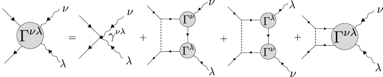
Figure 9: The diagrammatical representation of the second-order extension of the Bethe-Salpeter equation.

In principle, by similarly calculating for higher-order cases, it is possible to derive any full photon vertex in BCS superconductors.

At higher orders, it becomes more complicated to obtain the full photon vertex by solving the integral equations. In some cases, it is possible to avoid explicitly solving the integral equations using the diagrammatic method. As an example, we calculate the second-order response kernel. Let us focus on the term involving the full two-photon vertex and the triangular diagrams in the second-order response kernel in Eq. (37). The corresponding diagrams are shown in the first line of Fig. 10. We can sequentially substitute Eq. (181) into them, and it can be shown that

$$\frac{1}{2}\mathrm{Tr}\bigg{[}\gamma^{\mu}(\overline{k}+q,-q)G(\overline{k}+q)\Gamma^{\nu\lambda}(\overline{k},q_{1},q_{2})G(\overline{k})\bigg{]}$$

$$+\mathrm{Tr}\bigg{[}\gamma^{\mu}(\overline{k}+q,-q)G(\overline{k}+q)\Gamma^{\lambda}(\overline{k}+q_{1},q_{2})G(\overline{k}+q_{1})\Gamma^{\nu}(\overline{k},q_{1})G(\overline{k})\bigg{]}+[(\nu,q_{1})\leftrightarrow(\lambda,q_{2})]$$

$$= \frac{1}{2}\mathrm{Tr}\big{[}\Gamma^{\mu}(\overline{k}+q,-q)G(\overline{k}+q)\gamma^{\nu\lambda}(\overline{k},q_{1},q_{2})G(\overline{k})\big{]}$$

$$+\mathrm{Tr}\bigg{[}\Gamma^{\mu}(\overline{k}+q,-q)G(\overline{k}+q)\Gamma^{\lambda}(\overline{k}+q_{1},q_{2})G(\overline{k}+q_{1})\Gamma^{\nu}(\overline{k},q_{1})G(\overline{k})\bigg{]}+[(\nu,q_{1})\leftrightarrow(\lambda,q_{2})].$$ (182)

This equation can be easily translated into Feynman diagrams presented in Fig. 10.

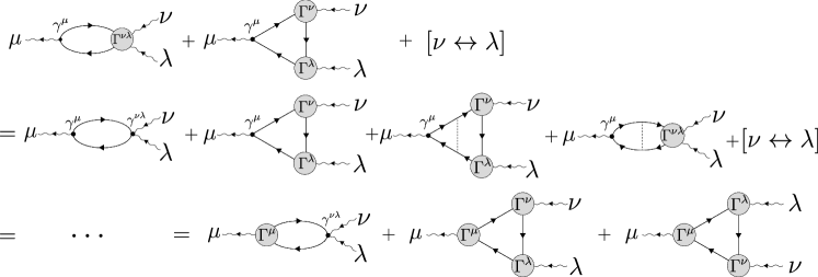
Figure 10: The diagrammatic representation of the calculation of the second-order response kernel. The last equality can be obtained by the Bethe-Salpeter equation. We can avoid explicitly solving the integral equation for the full two-photon vertex.

If we adopt the self-energy in Eq. (179), it is possible to calculate the second-order response without explicitly solving the integral equation for the full two-photon vertex, given the full one-photon vertex. In the previous study [28], the second-order response kernel is calculated in this way instead of explicitly using the full two-photon vertex. Although this simplification of the calculation is useful, we will not adopt the Fock approximation due to the subtlety explained in the main text.

Appendix C The detailed calculation of the correction part of the full two-photon vertex

In this appendix, we discuss the full two-photon vertex by the generalized CFOP method. The correction part of the full two-photon vertex is defined by

$$\Lambda^{\nu\lambda}(x,y,w_{1},w_{2})=\left.\frac{\delta^{2}\Sigma_{A}(x,y)}{\delta A_{\nu}(w_{1})\delta A_{\lambda}(w_{2})}\right|_{A=0}.$$ (183)

Since the self-energy of superconductors is the gap function, we have to calculate the functional derivative of $\Delta_{i,l,A}(x,y)$. The functional derivative of the gap equation leads to

$$\left.\frac{\delta^{2}\Delta_{i,l,A}(x,y)}{\delta A_{\nu}(w_{1})\delta A_{\lambda}(w_{2})}\right|_{A=0}$$

$$=-\frac{g_{l}\delta(x-y)}{2}\frac{\delta^{2}}{\delta A_{\nu}(w_{1})\delta A_{\lambda}(w_{2})}\left.\mathrm{Tr}\bigg{[}\tau_{i}\otimes E_{ll}G_{A}(x,y)\bigg{]}\right|_{A=0}$$

$$=\frac{g_{l}\delta(x-y)}{2}\functionalderivative{A_{\nu}(w_{1})}\left.\mathrm{Tr}\bigg{[}\tau_{i}\otimes E_{ll}G_{A}(x,\bar{z_{1}})\functionalderivative{G_{A}^{-1}(\bar{z_{1}},\bar{z_{2}})}{A_{\lambda}(w_{2})}G_{A}(\bar{z_{2}},y)\bigg{]}\right|_{A=0}$$

$$=-\frac{g_{l}\delta(x-y)}{2}\mathrm{Tr}\bigg{[}\tau_{i}\otimes E_{ll}G(x,\bar{z_{3}})\Gamma^{\nu}(\bar{z_{3}},\bar{z_{4}},w_{1})G(\bar{z_{4}},\bar{z_{1}})\Gamma^{\lambda}(\bar{z_{1}},\bar{z_{2}},w_{2})G(\bar{z_{2}},y)\bigg{]}$$

$$\qquad-\frac{g_{l}\delta(x-y)}{2}\mathrm{Tr}\bigg{[}\tau_{i}\otimes E_{ll}G(x,\bar{z_{1}})\Gamma^{\nu\lambda}(\bar{z_{1}},\bar{z_{2}},w_{1},w_{2})G(\bar{z_{2}},y)\bigg{]}$$

$$\qquad-\frac{g_{l}\delta(x-y)}{2}\mathrm{Tr}\bigg{[}\tau_{i}\otimes E_{ll}G(x,\bar{z_{1}})\Gamma^{\lambda}(\bar{z_{1}},\bar{z_{2}},w_{2})G(\bar{z_{2}},\bar{z_{3}})\Gamma^{\nu}(\bar{z_{3}},\bar{z_{4}},w_{1})G(\bar{z_{4}},y)\bigg{]}.$$ (184)

Assuming the functional derivative of the gap function takes the form

$$\left.\frac{\delta^{2}\Delta_{i,l,A}(x,y)}{\delta A_{\nu}(w_{1})\delta A_{\lambda}(w_{2})}\right|_{A=0}=\Lambda_{il}^{\nu\lambda}(x,w_{1},w_{2})\delta(x-y),$$ (185)

we obtain the matrix equation in the momentum space

$$\frac{2}{g_{i}}\Lambda_{il}^{\nu\lambda}(q_{1},q_{2})+\sum_{j,l^{\prime}}\mathrm{Tr}\bigg{[}\tau_{i}\otimes E_{ll}G(\bar{k}+q)\tau_{j}\otimes E_{l^{\prime}l^{\prime}}G(\bar{k})\bigg{]}\Lambda_{jl^{\prime}}^{\nu\lambda}(q_{1},q_{2})$$

$$=-\mathrm{Tr}\bigg{[}\tau_{i}\otimes E_{ll}G(\bar{k}+q)\gamma^{\nu\lambda}(\bar{k},q_{1},q_{2})G(\bar{k})\bigg{]}-\mathrm{Tr}\bigg{[}\tau_{i}\otimes E_{ll}G(\bar{k}+q)\Gamma^{\lambda}(\bar{k}+q_{1},q_{2})G(\bar{k}+q_{1})\Gamma^{\nu}(\bar{k},q_{1})G(\bar{k})\bigg{]}$$

$$\qquad-\mathrm{Tr}\bigg{[}\tau_{i}\otimes E_{ll}G(\bar{k}+q)\Gamma^{\nu}(\bar{k}+q_{2},q_{1})G(\bar{k}+q_{2})\Gamma^{\lambda}(\bar{k},q_{2})G(\bar{k})\bigg{]}.$$ (186)

This equation can be solved given the full one-photon vertices $\Gamma^{\mu}(k,q)$.