A Non-Parametric Approach to Heterogeneity Analysis

Abstract

This paper introduces a network-based method to capture unobserved heterogeneity in consumer microdata. We develop a permutation-based approach that repeatedly samples subsets of choices from each agent and partitions agents into jointly rational types. Aggregating these partitions yields a network that characterizes the unobserved heterogeneity, as edges denote the fraction of times two agents belong to the same type across samples. To evaluate how observable characteristics align with the heterogeneity, we implement permutation tests that shuffle covariate labels across network nodes, thereby generating a null distribution of alignment. We further introduce various network-based measures of alignment that assess whether nodes sharing the same observable values are disproportionately linked or clustered, and introduce standardized effect sizes that measure how strongly each covariate “tilts” the entire network away from random assignment. These non-parametric effect sizes capture the global influence of observables on the heterogeneity structure. We apply the method to grocery expenditure data from the Stanford Basket Dataset.

JEL: D11, C6, C14, C38

Keywords: Revealed Preferences, Preference Heterogeneity, Network Analysis, Permutation Methods

1 Introduction

In applied microeconometrics, the standard approach to modeling heterogeneity is to pool data across agents and decompose behavior into a common component plus an idiosyncratic term. While popular for its simplicity and interpretability, such a pooling approach often leaves a substantial behavioral variation unexplained. An alternative partitioning approach is proposed by Crawford and Pendakur (2012), who use revealed preference (RP) conditions to group individuals whose data can be jointly rationalized by a common economic model. Rather than assuming a single parametric specification for an entire population, this method classifies agents into subsets—types—each satisfying a standard revealed-preference axiom such as the Generalized Axiom of Revealed Preferences (GARP). This approach systematically captures all observed heterogeneity, but it does so in a coarse, categorical way. Two individuals either belong to the same type or not, without a notion of distance across types that would signal “how close” or “how different” they are in their decision patterns. By contrast, in a parametric setting, distance in parameter space can naturally quantify the degree of heterogeneity; the partitioning method, while comprehensive, lacks such a concept.

In this paper, we build on the partitioning methodology of Crawford and Pendakur (2012) and aim to provide a finer-grained understanding of heterogeneity—one that also connects unobserved differences in behavior to observable covariates. To do so, we propose a permutation-based approach that derives a similarity network for the population. Specifically, rather than requiring each agent’s entire history of choices to be lumped into a single type, we repeatedly form synthetic datasets by randomly sampling the same number of decisions from each agent. In each synthetic dataset, we run a partitioning procedure that classifies individuals into types consistent with GARP (or another RP axiom). We then record whether two agents end up in the same type. Repeating this procedure over many samples yields a probabilistic adjacency matrix: the similarity between any two agents is the fraction of synthetic datasets in which they share the same type.

Our partitioning approach draws on the Mixed Integer Linear Programming (MILP) methods of Heufer and Hjertstrand (2015) and Demuynck and Rehbeck (2023) for computing goodness-of-fit measures. We adapt an MILP algorithm for computing the Houtman and Maks index to our setting: in each synthetic dataset, the procedure identifies the largest GARP-consistent subset of individuals and removes them from the dataset. We then repeat the procedure on the remaining individuals until no further GARP-consistent subsets can be found. This yields a partition of the population into disjoint subgroups, each satisfying the RP restrictions. Across many synthetic datasets, we record how often any two individuals appear in the same GARP-consistent group, thereby constructing a similarity matrix $G$. Specifically, $G_{i,j}$ is the fraction of synthetic datasets in which agents $i$ and $j$ share a subgroup. Finally, we apply a thresholding rule to $G$ to obtain a family of adjacency matrices $H^{\alpha}$ for various significance levels $\alpha$. In $H^{\alpha}$, two individuals are linked if we cannot reject the hypothesis that they belong to the same type at precision level $\alpha$, as they co-occur together in a fraction at least $1-\alpha$ of the datasets.

Our approach transforms a purely combinatorial partition problem into a network structure that captures partial overlaps, allowing us to study heterogeneity in a more granular way than a single, global partition would permit. Indeed, in a single partition that lumps all of an individual’s choices together, certain pairs of agents may never be assigned to the same type if any of their decisions conflict. By contrast, when we repeatedly sample a few choices from each agent, those conflicting decisions might be excluded from some draws, allowing otherwise “incompatible” agents to appear together in a GARP-consistent subset. Over many draws, these partial overlaps yield a richer notion of “closeness,” in contrast to a strict partitioning approach that must categorize such agents as either always separate or always together.

From here, we can leverage standard network tools to measure “distance” between agents without relying on parametric assumptions. For instance, path length between two agents who do not share a direct link can capture indirect similarity if they both connect to the same intermediary. We can also compute centrality measures to identify agents acting as “bridges,” and run community detection algorithm to discover subgroups sharing overlapping though not identical behaviors. In this way, our framework bridges the gap between parametric and non-parametric approaches: partitioning ensures that we use minimal assumptions about preferences, while our permutation-based approach incorporates a spectrum of partial overlaps akin to the continuous heterogeneity favored in pooling approaches.

Beyond describing unobserved heterogeneity, our framework also connects it to observables. Standard microeconometric approaches typically ask: “Does income (or age, or family size, etc.) explain why agents fall into different preference types?”—often by embedding demographic variables in a structural or regression model. By contrast, our method views similarity as revealed by the data themselves, then asks whether agents with a given demographic characteristic systematically cluster together (or occupy similar positions) in the resulting similarity network. Concretely, we propose a permutation test that first computes a baseline measure of how strongly a covariate “explains” similarity. We consider four kinds of network-based similarity measures: (i) pairwise similarity—do agents with the same observable form disproportionately many direct links? (ii) community detection—do they tend to appear in the same network communities? (iii) entropy—how diverse or homogeneous are communities with respect to this covariate? and (iv) degree centrality—do agents with a particular observable occupy especially central positions in the network? We then generate a null distribution by shuffling observable labels across nodes (while keeping the similarity network intact). Comparing the actual measure of alignment to its distribution under random shuffles yields a statistical test telling us whether an observable systematically explains where individuals stand in the similarity network.

Finally, we introduce a standardized effect size (akin to a Z-score) that reflects how many standard deviations the observed similarity measure deviates from the random-assignment benchmark. This quantity captures the global, non-parametric influence of a covariate on the heterogeneity structure. By contrast with parametric coefficients—which can be limited or biased by their underlying model assumptions—our effect size offers a broader perspective: it quantifies how strongly a covariate “tilts” the entire unobserved heterogeneity structure, as mapped out by the similarity networks, away from what would be expected under random assignment.

With this approach, observed heterogeneity can be measured at various levels. The Pairwise similarity captures the degree of similarity of connected nodes in terms of their observable values. The Community Detection Consistency measure goes one step further. Instead of focusing solely on individual links, it evaluates whether nodes sharing the same observables tend to cluster together into well-defined communities. This captures a more global notion of alignment. The Entropy measure examines the distribution of observables across communities. Hence, even if a particular variable has no significant effect on direct links, it may still affect the network structure at a more aggregated level by shaping the composition or diversity of these communities.

We apply our framework to grocery expenditure data from the Stanford Basket Dataset used, among others, by Bell and Lattin (1998), Shum (2004), Hendel and Nevo (2006a, b), and Echenique, Lee and Shum (2011). The data used in this paper comprise 57,077 transactions by 400 households across 368 product categories in four grocery stores over 104 weeks (aggregated into 26 monthly periods). For each household, we construct $T=50$ synthetic datasets by randomly sampling one consumption vector from its 26 observed choices. In each synthetic dataset, we partition the agents into types using our Mixed Integer Linear Programming (MILP) algorithm. We then aggregate these results into a probabilistic similarity matrix $G$, which records how often any pair of households co-occurs in the same subset across all synthetic datasets.

After constructing the similarity matrix $G$, we apply our thresholding procedure to obtain a family of adjacency matrices $H^{\alpha}$ for different significance levels $\alpha\in\{5\%,10\%,15\%,20\%\}$. In $H^{5\%}$ for example, a link exists between $i$ and $j$ if these households belong to the same type in at least $95\%$ of the synthetic datasets. We find that the density function of the empirical distribution of the coefficient values in $G$ is single-peaked, centered on 74%, with a standard deviation of about 1%. This tight distribution indicates a high level of consistency across households. Additionally, we find that the networks $H^{\alpha}$ consistently feature a single dominant component. For $\alpha=20\%$, we find that 90% households are connected in the main component. This indicates that, despite differences in decision patterns, households share sufficient overlap in their revealed preferences to form a cohesive network structure. This finding reinforces the results of Crawford and Pendakur (2012), who used a minimum partitioning approach to identify four to five distinct consumption types in a sample of 500 observations. In their analysis, 2/3 of observations were classified into a single type, with two types explaining 85% of the data. By adopting a permutation-based approach, we uncover a more nuanced and interconnected structure. Although households might appear incompatible under a strict partitioning scheme, they still form a cohesive network rather than disjoint clusters.

We then evaluate how various household characteristics align with the structure of $H^{\alpha}$. Specifically, for each covariate, we permute it randomly $1,000$ times across the network nodes and compare the resulting alignment measures to those observed in the real data, thereby testing whether the covariate is truly predictive of similarity patterns. We further quantify deviations from randomness by computing effect sizes for each alignment metric. We find that certain covariates stand out with large standardized effect sizes (measured in standard deviations from the random-permutation baseline) and are rejected in fewer than 1% of the randomizations. For example, households with 1 to 2 individuals record effect sizes on the order of 4.9 to 5.7 standard deviations in Pairwise Similarity, indicating that they connect disproportionately often to other small-family households relative to random assignment. Older households also exhibit effect sizes of approximately 2.3 to 3.2 in this metric, again at the 1% significance threshold, suggesting they form tightly knit subgroups well beyond chance. Turning to Community Detection, these same covariates remain significant, implying that their members cluster together in larger-scale communities. By contrast, the Entropy measure shows that medium-to-large family-size households, as well as younger households—while not forming such tight subgroups—are associated with notably higher community-level diversity (with positive effect sizes in the 1.2–2.8 range). Finally, Degree Centrality reveals that younger, and medium-to-large family-size households act as “bridges” in the network, scoring several standard deviations above the null benchmark and reinforcing the notion that heterogeneity can arise both in localized clusters and through global connectivity.

Next, we extend our approach in several ways. First, we examine whether the identified patterns remain stable when we account for seasonality. We split each household’s consumption choices by season and construct a larger set of “season-households,” then apply our network-based analysis to this expanded sample. Specifically, for computational reasons, we first focus on a subsample of 100 households, and divide each households into four “season-households”—summer, autumn, winter, and spring—creating a total of 400 season-households. We then apply the same similarity-network procedure as before to determine whether the resulting links reflect stable, household-level preferences or instead vary significantly with seasonal labels.

Our findings indicate that households remain tightly linked to themselves across seasons. The household indicator variable consistently shows large and highly significant effect sizes in both Pairwise Similarity and Community Detection. Such a result underscores that each household’s seasonal observations cluster more with each other than we would ever expect under random assignment, reinforcing the idea that underlying preferences remain relatively stable across seasons. By contrast, only the spring season indicator exhibit meaningful deviations from randomness for the community detection and entropy metrics. This suggests that while households might alter their consumption in minor ways across seasons - and especially in spring - these adjustments do not substantially reorganize the overall structure of heterogeneity in the network.

We also consider that a single household’s decisions need not all originate from a single decision model—households may contain multiple “situational dictators” (e.g., different family members, Cherchye, de Rock and Vermeulen (2007)) or adapt to evolving needs over time. To investigate this possibility, we isolate multiple internally GARP-consistent “type-households” within each family and embed these smaller decision units in our similarity-network analysis. For computational reason, we first focus on a subsample of 200 households, and divide each households into internally GARP-consistent “type-households”, applying our partitioning approach. We end up with a larger sample of 372 “household-types”, where 81% of the households are described by two decision-models, 16.5% by one, and the remaining 2.5% by three. We apply our network-based analysis to this sample, and find that the explanatory power of some observables becomes more muted overall, particularly at the $\alpha=5\%$ precision level. Certain patterns emerge when $\alpha=10\%$. In particular, the “Household” label has a strong predictive power for Pairwise Similarity and Community Detection, with effect sizes, in the 1.4–2.8 range (in standard deviations), suggesting that multiple subtypes within the same household are closer to one another than random assignment would imply.

Finally, we compare our main partitioning procedure—which, in each synthetic dataset, seeks the single largest GARP-consistent subset—with a minimum partitioning approach aiming to cover the data with as few GARP-consistent subsets as possible. Indeed, it is possible that our procedure over-fragments the population, creating too many small types in instances where a smaller number of larger, GARP-consistent sets could suffice. To assess whether these potential differences affect our empirical findings, we formulate and solve an MILP problem that builds a minimal partition into GARP-consistent subsets. Although this minimum-partitioning approach is computationally heavy for large datasets, we successfully implement it on a subsample of 100 households. We then compare the resulting network structure and effect sizes to those obtained from our main procedure. Both methods lead to broadly consistent results in terms of network characteristics, and alignment of households’ characteristics with the structure of the similarity networks.

The closest paper to ours is Cherchye, Saelens and Tuncer (2024). Drawing on the minimum partition approach of Cosaert (2019), Cherchye, Saelens and Tuncer (2024) quantify the contribution of observable consumer characteristics to describing preference heterogeneity. The idea of their approach is to compare the distribution of a given characteristic values with the distribution of types obtained from the minimum partition approach of Cosaert (2019). While we share with Cherchye, Saelens and Tuncer (2024) the common objective of quantifying the contribution of observable characteristics to describing preference heterogeneity, we do so in different ways. Our approach first constructs a network representation of unobserved heterogeneity by aggregating GARP-consistent partitions across multiple synthetic datasets. We then evaluate whether observable characteristics are systematically associated with similarities within this network through statistical hypothesis testing and non-parametric effect size quantification. This allows us to assess the significance and magnitude of each covariate’s influence on the heterogeneity structure. Additionally, Seror (2024a) applies the permutation approach introduced in this paper to explore heterogeneity in moral reasoning across multiple large language models. Finally, we specifically contribute to the studies on minimum partitioning approaches applied to microdata (Cosaert (2019), Crawford and Pendakur (2012)) by providing a Mixed Integer Linear Programming (MILP) formulation of this optimization problem. Our approach can be applied in cases where the number of dimensions exceeds $2$.

2 Non-Parametric Heterogeneity Analysis

We consider the standard consumer problem with $K$ goods. A decision maker chooses a bundle $q\in\mathbb{R}^{K}_{+}$ subject to a linear constraint where prices are given by a vector $p\in\mathbb{R}^{k}_{+}$. The theory is extended to more general choice environments in Section 3. Let $\mathcal{I}$ denote a set of agents, $\mathcal{N}_{i}=\{1,\dots,N_{i}\}$ a set of observations for agent $i$, $\mathcal{N}=\{n_{i}\}_{i\in\mathcal{I},n_{i}\in\mathcal{N}_{i}}$ the set combining all observations, and $D_{i}=\{p^{n}_{i},q^{n}_{i}\}_{n\in\mathcal{N}_{i}}$ the set of data for agent $i$. $\mathcal{A}^{n}_{i}\subset\mathbb{R}^{K}_{+}$ denotes the choice set of agent $i$ in observation $n\in\mathcal{N}_{i}$. The index $i$ is dropped when not necessary.

2.1 Revealed Preference Conditions

The following definitions characterize the revealed preference conditions:

Definition 1.

Let $e=\{e^{n}\}_{n\in\mathcal{N}_{i}}\in[0,1]^{N_{i}}$. For agent $i\in\mathcal{I}$, bundle $q^{n}$ is

1. $e$-directly revealed preferred to a bundle $q$, denoted $q^{n}R^{0}_{e}q$, if $e^{n}p^{n}q^{n}\geq p^{n}q$ or $q=q^{n}$.

2. $e$-directly revealed strictly preferred to a bundle $q$, denoted $q^{n}P^{0}_{e}q$, if $e^{n}p^{n}q^{n}>p^{n}q$ or $q=q^{n}$.

3. $e$-revealed preferred to a bundle $q$, denoted $q^{n}R_{e}q$, if there exists a sequence of observed bundles $q^{j},\dots,q^{m}$ such that $q^{n}R^{0}_{e}q^{j}$, …$q^{m}R^{0}_{e}q$.

4. $e$-revealed strictly preferred to a bundle $q$, denoted $q^{n}P_{e}q$, if there exists a sequence of observed bundles $q^{j},\dots,q^{m}$ such that $q^{n}R^{0}_{e}q^{j}$, …$q^{m}R^{0}_{e}q$, and at least one of them is strict.

We can define the $e$-generalized axiom of revealed preference (GARP_e) as follows:

Definition 2.

(GARP_e). Let $\mathcal{T}$ a finite set of observations, and $(p^{t},q^{t})_{t\in\mathcal{T}}$ a dataset. $(p^{t},q^{t})_{t\in\mathcal{T}}$ satisfies the Generalized Axiom of Revealed Preference (GARP_e) if for all sequence of observations $t_{1},\dots,t_{M}$ in $\mathcal{T}$:

$$q^{t_{1}}R_{e}^{0}q^{t_{2}}R_{e}^{0}\dots R_{e}^{0}q^{t_{M}}\text{ implies not }q^{t_{M}}P_{e}^{0}q^{t_{1}}$$

When $e=\{1\}_{t\in\mathcal{T}}$, this definition is the standard definition of GARP from Varian (1982). A finite data set $D=(p^{t},q^{t})_{t\in\mathcal{T}}$ is rationalizable by a model of utility maximization if and only if it satisfies the GARP₁ condition (Afriat (1967)), making GARP a reference for measuring rationality in the literature. Additionally, vector $e$ acts as a precision vector, as if GARP_e is satisfied, then GARP_v is also satisfied, with $v^{n}\leq e^{n}$ for all $n\in\mathcal{N}_{i}$ (Halevy, Persitz and Zrill (2018)). Hence, it is possible to aggregate the vector $e$ in various ways to measure the extent of GARP violations through rationality indices (Halevy, Persitz and Zrill (2018)).

2.2 Partitioning Approach

Let $B\subseteq\mathcal{I}$ denote a subset of agents. Let $\mathcal{D}=\{p^{n}_{i},q^{n}_{i}\}_{n\in\mathcal{N}_{i},i\in B}$ denote the dataset that combines the decisions of all the agents in set $B$. The largest subset of agents that jointly satisfy the aggregate condition of Definition 2 can be characterized as follows:

$$LS(e_{B})=\operatorname*{arg\,max}_{B\subseteq\mathcal{I}}\mid B\mid\text{ s.t. }\{q^{n}_{i},\mathcal{A}^{n}_{i}\}_{n\in\mathcal{N}_{i},i\in B}\text{ satisfies }GARP_{e_{B}},$$ (1)

where $\mid B\mid$ measures the number of elements in set $B$, and $e_{B}=\{e^{n}_{i}\}_{n\in\mathcal{N}_{i},i\in B}\in[0,1]^{N_{b}}$, with $N_{b}=\sum_{i\in B}N_{i}$. From this point, it is possible to build a recursive procedure that partitions the set of agents $\mathcal{I}$ by repeating the optimization problem (1):

Procedure 1.

• Step 1: Find the subset $LS_{1}(e_{1})$ that solves (1).

• Step 2: If $\mathcal{I}\setminus LS_{1}(e_{1})=\phi$, stop. Otherwise, set $\mathcal{I}=\mathcal{I}\setminus LS_{1}(e_{2})$, and find the subset $LS_{2}(e_{2})$ that solves (1).

• Step 3: If $\mathcal{I}\setminus LS_{2}(e_{2})=\phi$, stop. Otherwise, set $\mathcal{I}=\mathcal{I}\setminus LS_{2}$, and find the subset $LS_{3}(e_{3})$ that solves (1).

• …

This procedure partitions the set of agents $\mathcal{I}$ into subsets. In each subset $LS_{k}$, decisions satisfy GARP${}_{e_{k}}$, and $LS_{k}$ is the $k$th subset in the partition of $\mathcal{I}$ according to Procedure 1:

$$\mathcal{I}=\{LS_{k}\}_{k\in\{1,\dots,K\}},\text{ with }K\leq I,$$

Let $e_{k}=\{e\}_{n\in\mathcal{N}_{i},i\in LS_{k}}$ for any subset $LS_{k}$, and $e\in[0,1]$. If $e$ is set to $0$, then all agents are grouped into the same type, as the revealed preference conditions are not restrictive. When $e=1$, then it is required for all agents to satisfy GARP₁. In the context of optimization (1), $e$ can be interpreted as a level of precision, as there always exists a threshold $e(i,j)\geq 0$ such that if $e$ is lower than this threshold, then agents $i$ and $j$ belong to the same type.

One key challenge with optimization (1) is its computational complexity, as it may not admit a solution in polynomial time. Specifically, optimization (1) is akin to the task of determining the Houtman and Maks Index, which identifies the maximum number of observations in a dataset that jointly satisfy GARP₁. However, the two problems differ in their scope: optimization (1) aims to identify the largest subset of individuals whose aggregated decisions satisfy GARP_e. If there is only one observation per individual, the two problems are equivalent when $e=1$, because the set of observations directly corresponds to the set of individuals. In this case, finding the HMI in a dataset aggregating decisions across individuals is formally equivalent to finding the maximum set of individuals that are jointly rational. When individuals contribute multiple observations, the problems diverge slightly although the underlying logic remains similar.

Drawing on the approaches of Heufer and Hjertstrand (2015) and Demuynck and Rehbeck (2023) for computing the HMI, it is possible to find a mixed integer linear programming approach for solving (1). The corollary below gives an MILP formulation of optimization problem (1):

Proposition 1.

The following MILP computes the set $LS(e)$:

$$LS(e)=\operatorname*{arg\,max}_{\mathbf{x},\mathbf{\psi},\mathbf{U}}\mid B\mid,$$

subject to the following inequalities:

$$U^{n}-U^{k}<\psi^{n,k}\text{ for all }(n,k)\in\mathcal{N}^{2}$$ (IP 1)

$$\psi^{n,k}-1\leq U^{n}-U^{k}\text{ for all }(n,k)\in\mathcal{N}^{2}$$ (IP 2)

$$x_{i(n)}e^{n}p^{n}.q^{n}-p^{n}.q^{k}<\psi^{n,k}A\text{ for all }(n,k)\in\mathcal{N}^{2}$$ (IP 3)

$$(\psi^{n,k}-1)A\leq p^{k}.q^{n}-x_{i(k)}e^{k}p^{k}.q^{k}\text{ for all }(n,k)\in\mathcal{N}^{2},$$ (IP 4)

where $\mathbf{U}=\{U^{n}\}_{n\in\mathcal{N}}$, $U^{n}\in[0,1)$, $\mathbf{x}=\{x_{i}\}_{i\in\mathcal{I}}$, $x_{i}\in\{0,1\}$, $\mathbf{\psi}=\{\psi^{n,k}\}_{n,k\in\mathcal{N}}$, $\psi^{n,k}\in\{0,1\}$, $i(n)\in\mathcal{I}$ is the agent making decision $n\in\mathcal{N}$, $e=\{e^{n}\}_{n\in\mathcal{N}}$, and $A>\max_{n\in\mathcal{N}}p^{n}q^{n}$.

Proof.

The proof is in Appendix A.1 ∎

2.3 Permutation approach

The sharp classification that can be build using optimization (1) and Procedure 1 only indicates whether agents belong to the same type, without offering insights into the closeness of agents that do not fall into the same type. To better understand the similarity between different agents’ reasoning, it is useful to adopt a probabilistic approach that assesses the degree of closeness between agents. Below, we designed a permutation approach that evaluates the similarity of decisions between pairs of agents based on RP restrictions. We proceed in two steps.

In the first step, the method generates $T$ synthetic datasets, denoted as $\hat{D}_{t}$ for $t\in\mathcal{T}=\{1,\dots,T\}$. Each synthetic dataset $\hat{D}_{t}$ is constructed by randomly sampling $s_{i}\leq N_{i}$ decisions from each agent $i$ in $\mathcal{I}$, ensuring that the synthetic data equally represent all agents. In the second step, for each synthetic dataset $\hat{D}_{t}$, Procedure 1 and the MILP optimization from Proposition 1 are applied.

Let $\delta_{i,j}^{t}\in\{0,1\}$ be an indicator variable equal to 1 if agents $i$ and $j$ are classified as the same type in dataset $\hat{D}_{t}$, and 0 otherwise. The outcome of this procedure is a probabilistic network matrix $G=\{G_{i,j}\}_{i,j\in\mathcal{I}}$, defined as:

$$G_{i,j}=\frac{1}{T}\sum_{t=1}^{T}\delta_{i,j}^{t}.$$ (2)

The coefficient $G_{i,j}$ represents the proportion of times agents $i$ and $j$ are classified as the same type across all synthetic datasets, providing a measure of how frequently these agents align in terms of their revealed preference restrictions. Hence, we can interpret $G_{i,j}$ as measuring the statistical similarity between agents $i$ and $j$.

Several points are in order. First, the coefficient $G_{i,j}$ does not measure the direct similarity of decisions. In fact, the decisions of agents $i$ and $j$ can be substantially different but still jointly satisfy RP restrictions. Hence, this methodology is intrinsically different from clustering methods that rely on observable similarities, such as $K$-means or hierarchical clustering. For example, $K$-means clusters agents based on their proximity in a predefined feature space. Similarly, hierarchical clustering builds a nested partition of agents by iteratively merging those with the smallest distances between them in a feature space. These methods rely on predefined metrics of similarity.

Using the similarity coefficients $G_{i,j}$, it is also possible to build a statistical approach that distinguishes between two hypothesis:

• $H_{0}$: $i$ and $j$ belong to the same type within the set $\mathcal{I}$.

• $H_{1}$: $i$ and $j$ do not belong to the same type within the set $\mathcal{I}$.

We can then use the following procedure to differentiate between different types:

Procedure 2.

Let $\alpha\in(0,1)$. For any pair of agents $i,j\in\mathcal{I}$, reject $H_{0}$ in favor of $H_{1}$ at the significant level $\alpha$ if the fraction of synthetic datasets that satisfy $\delta_{i,j}^{t}=0$ for $t\in\{1,\dots,T\}$ is weakly smaller than $\alpha$, or $\phi_{\alpha}=1$ with

$$\phi_{\alpha}=\begin{cases}1\text{ if }\mid\{t\in\mathcal{T}:\delta_{i,j}^{t}=0\}\mid/T\leq\alpha\\ 0\text{ otherwise.}\end{cases}$$

Using Procedure 2, it is possible to build a network $H^{\alpha}$ out of network $G$, where

$$H_{i,j}^{\alpha}=\begin{cases}1\text{ if $i$ and $j$ belong to the same type at the $\alpha$ precision level}\\ 0\text{ otherwise.}\end{cases}$$

In matrix $H^{\alpha}$, two agents are linked if we cannot reject the assumption $H_{0}$ at the $\alpha$ precision level, meaning that $i$ and $j$ do not belong to the same type in less than a fraction $\alpha$ of the synthetic datasets $\hat{D}_{t}$, $t\in\{1,\dots,T\}$.

Discussion

The analysis of network matrices $G$ or $H^{\alpha}$ aligns with traditional microeconometric (parametric) analysis, as its goal to uncover underlying structures of heterogeneity, yet it reframes this question without the need for observable covariates. Unlike the standard pooling approach, which relies on demographic or socioeconomic factors to explain behavioral variations, the $G$ and $H^{\alpha}$ matrices capture probabilistic alignments among agents, allowing similarities and differences to emerge organically from the data itself. Relative to matrix $G$, matrix $H^{\alpha}$ might be relatively easier to interpret as it is made of binary coefficients, so it is possible to compute standard network metrics.

In this approach, parameter $s=\{s_{i}\}_{i\in\mathcal{I}}$ corresponds to the number of observations sampled for each individual in the procedure. The value of $s$ directly influences the similarity matrix $G$, as it determines the extent to which individual observations are compared across agents. Specifically, $G(i,j)$ measures the frequency with which $s_{i}$ observations from agent $i$ are consistent with $s_{j}$ observations from agent $j$, given the revealed preference restrictions. A higher value of $s$ implies a stricter test of compatibility, as more observations are included in the comparison. In the case where $s_{i}=N_{i}$ for all $i$, $G$ is a deterministic representation of the partition of agents into types built using Procedure 1. The resulting network $G$ can be characterized as a set of fully connected components, where each component corresponds to a type, as defined by Procedure 1. In the case where $s_{i}=1$ for all $i\in\mathcal{I}$, the similarity matrix $G$ captures a pairwise metric of alignment between individual decisions rather than aggregate decision patterns. This case is particularly interesting, as it is possible to use a precision vector $e=\{1\}_{n\in\mathcal{N}_{i(n)},i\in\mathcal{I}}$ in Procedure 1. For intermediate cases where $s_{i}\leq N_{i}$, the permutation approach introduces flexibility into the comparison, allowing for the emergence of links between agents who are not completely aligned in their decision-making patterns. These links provide a notion of distance between individuals, enabling the identification of partial similarities that would be missed in the strict partitioning approach.

Transitivity in network links in $H^{\alpha}$ is not necessarily guaranteed when $s_{i}<N_{i}$. As a result, it is possible to identify indirect similarities between agents who do not share direct links but are connected through common intermediaries, revealing more nuanced structures of behavioral alignment that would be missed by strict partitioning methods. In particular, the lack of transitivity opens the door to measuring “distances” between agents: for instance, the path length from one agent to another can capture the idea that two agents are indirectly similar through a third. We can also leverage centrality measures to pinpoint agents who serve as key “bridges” in connecting different types, or employ clustering algorithms to detect subgroups of agents who exhibit overlapping—though not identical—behaviors. Such methods highlight how partial alignment and indirect connections can yield a richer, more fine-grained understanding of heterogeneity in networks.

To see why transitivity is not guaranteed in network $H^{\alpha}$, consider the example of Table 1. There are three agents, $A$, $B$, $C$, making two decisions. The following pairs of decisions violate the Weak Axiom of Revealed Preferences (WARP): $(x,z)$, $(y,w)$, and $(z,w)$. Agents $B$ and $C$ can never belong to the same type, since $(z,w)$ violate WARP. Agents $A$ and $B$ belong to the same type in half of the synthetic datasets, as decision $x$ from agent $A$ will be drawn in about half of the synthetic datasets and $(x,z)$ does not violate WARP. Similarly, agents $A$ and $C$ belong to the same type in about half of the synthetic datasets. The resulting probabilistic network matrix $G$ is such that $G_{A,B}=G_{A,C}=0.5$, and $G_{A,C}=0$. There is no transitivity in the network links in $H^{0.5}$, as there is a link from $B$ to $A$, and a link from $A$ to $C$, but no link from $C$ to $B$. Intuitively, there is no transitivity because the similarity between $A$ and $B$ is based on a different subset of decisions than the similarity between $A$ and $C$.

2.4 Relevance of Observables in Explaining Heterogeneity: A Statistical Test

Section 2.3 introduces a probabilistic framework for constructing similarity networks $G$ and $H^{\alpha}$, which capture the alignment of agents’ preferences based solely on revealed preference (RP) restrictions. In this section, we extend this framework to evaluate the informativeness of observable characteristics, such as demographic or treatment variables, in explaining heterogeneity within the network. The objective of the tests below is to evaluate how strongly an observable characteristic, such as gender or income, aligns with the heterogeneity structure captured in $H^{\alpha}$. Specifically, we assess whether nodes sharing the same value for an observable $Z$ are disproportionately linked or clustered in $H^{\alpha}$, compared to what would be expected under random assignment of $Z$. Below, we outline the different metrics used, their computation, and interpretation.

Pairwise similarity $R(Z)$

A simple way to test alignment is to compute the proportion of links in $H^{\alpha}$ where both nodes share the same value for the observable $Z$. Let $Z_{i}$ denote the value of $Z$ for agent $i$. The observed alignment proportion is given by:

$$R(Z)=\frac{\text{Number of links where }Z_{i}=Z_{j}}{\text{Total number of links in }H^{\alpha}}.$$

A higher $R(Z)$ indicates that nodes with the same observable value $Z$ are more likely to be linked in the network.

Community Detection $C(Z)$

The community detection metric evaluates whether nodes with the same $Z$ disproportionately belong to the same community as identified by a community detection algorithm. Using the Louvain method for example, we can identify community memberships $\text{Comm}(i)$ for each node $i$. The observed alignment within communities is given by:

$$C(Z)=\frac{\text{Number of node pairs where }Z_{i}=Z_{j}\text{ and }\text{Comm}(i)=\text{Comm}(j)}{\text{Total node pairs in the same community}}.$$

Entropy of $Z$ Across Communities $H(Z)$

Entropy quantifies the spread of $Z$ across the communities detected in $H^{\alpha}$. For a community $c$, let $\mathcal{N}_{c}$ represent its nodes, and let $P(Z=z|c)$ denote the proportion of nodes in $\mathcal{N}_{c}$ with $Z=z$. The entropy of $Z$ within $c$ is given by:

$$H(Z|c)=-\sum_{z\in Z}P(Z=z|c)\log P(Z=z|c).$$

The overall entropy is a weighted sum across all communities:

$$H(Z)=\sum_{c}\frac{|\mathcal{N}_{c}|}{|\mathcal{N}|}H(Z|c),$$

where $|\mathcal{N}|$ is the total number of nodes. Lower entropy indicates that $Z$ values are concentrated within specific communities.

Degree Centrality $D(Z)$

Degree centrality measures the importance of nodes within a network based on their number of direct connections. Some variables might be particularly conducive to a high degree of connections relative to others. In the context of a binary variable $Z$, it is possible to measure the average degree of the nodes $i$ such that $Z_{i}=1$. Denoting $D_{i}$ the degree of node $i$, the average degree centrality for binary variable $Z$ is given by:

$$D(Z)=\frac{\sum_{i\in\mathcal{N}_{1}}D_{i}}{|\mathcal{N}_{1}|},$$

with $\mathcal{N}_{1}=\{i\in\mathcal{I}:Z_{i}=1\}$. A higher $D(Z)$ indicates that nodes with $Z=1$ occupy more central positions in the network, having a greater number of direct connections compared to networks.

Discussion

All of the measures introduced above provide a lens into how observable characteristics, such as $Z$, explain the heterogeneity structure in the network $H^{\alpha}$. However, they do so from distinct, and not necessarily overlapping, angles. The Pairwise similarity $R(Z)$ captures the direct, pairwise similarity of connected nodes in terms of their observable values. This measure is straightforward and interprets similarity purely in terms of immediate network neighbors having identical attributes. The Community Detection Consistency measure $C(Z)$ goes one step further: it aggregates local alignments into larger-scale structures. Instead of focusing solely on individual links, it evaluates whether nodes sharing the same $Z$-value tend to cluster together into well-defined communities. This captures a more global notion of alignment, where the variable $Z$ explains not just pairwise connections, but also the overarching division of the network into distinct groups. The Entropy measure $H(Z)$ examines the distribution of $Z$-values across communities. Even if nodes with the same $Z$-value cluster together, there may be several communities each dominated by similar values of $Z$, or conversely, communities that are more mixed. Entropy thus provides a sense of how concentrated or diffuse the attribute $Z$ is across the network’s communities, complementing the previous metrics by focusing on the diversity or homogeneity of node attributes within community partitions. Lastly, the Degree Centrality measure focuses on positional importance: do nodes that share a particular $Z$-value hold more central positions in the network? Even if these nodes do not form tight communities or always link preferentially with each other, they may nonetheless occupy hubs that dominate the network’s connectivity. This metric highlights a different dimension of network structure, emphasizing the prominence of certain attributes in shaping the network’s topology.

Procedure

Let $Z$ an observable for all agents in some vector space, and $M(Z)$ belongs to the set of metrics characterized previously. For each node $i$ in $H^{\alpha}$, we observe $Z_{i}$. The statistical test of relevance for observable $Z$ in explaining heterogeneity using metric $M(Z)$ distinguishes between two statistical hypothesis:

• $W_{0}$: Observable $Z$ has no effect on the observed heterogeneity.

• $W_{1}$: Observable $Z$ affect the observed heterogeneity.

Testing procedure. We generate a set of randomized networks $\{C^{t}\}_{t\in\{1,\dots,\tau\}}$ by shuffling the $Z$ labels across nodes while preserving the structure of $H^{\alpha}$. For each randomized network $C^{t}$, we compute the metric $M(Z)^{t}$, and build a null distribution of alignment proportions under the randomization.

Procedure 3.

Let $\gamma\in(0,1)$. Reject $W_{0}$ in favor of $W_{1}$ at the significance level $\gamma$ if $p\leq\gamma$, with

$$p=\mid\{t\in\{1,\dots,\tau\}:M(Z)^{t}\geq M(Z)\}\mid/\tau.$$

A significant p-value indicates that the observable $Z$ is not randomly assigned in the similarity network $H^{\alpha}$, but rather capture a relevant dimension of similarity between agents. It is worth noting that this test is applicable independently of the nature of the space where $Z$ resides, except for the centrality measure $D(Z)$, which is specific to binary variables. Indeed, the test relies on permutations of the labels rather than assumptions about their structure or distribution, making it versatile and robust to a variety of settings.

2.5 Non-Parametric Effect of Observables on Heterogeneity

To quantify the deviation from randomness, we can compute the effect size for each metric $M(Z)\in\{R(Z),C(Z),Z(Z),D(Z)\}$:

$$\beta=\frac{M(Z)-\mathbb{E}[M(Z)^{t}]}{\text{SD}[M(Z)^{t}]},$$ (3)

where $\mathbb{E}[M(Z)^{t}]$ and $\text{SD}[M(Z)^{t}]$ denote the mean and standard deviation of the alignment proportions under the null distribution. A larger effect size implies a stronger relationship between $Z$ and heterogeneity.

Here, the $\beta$ coefficient measures the standardized effect size of the observable $Z$ in explaining the similarity in network $H^{\alpha}$, based on observable $Z$. Specifically, it quantifies how much the observed alignment of $Z$ across network links deviates from what would be expected under random assignment, normalized by the variability in the null distribution. A higher $\beta$ value indicates that the observable has a strong and systematic relationship with the heterogeneity captured in the network, whereas a $\beta$ close to zero suggests that the observable contributes little to explaining preference patterns.

In contrast, in traditional parametric regressions, the corresponding measure reflects the marginal effect of an observable $Z$ on an outcome variable, conditional on the model’s other covariates. While regression coefficients estimate direct causal or associative relationships under specific functional form assumptions (e.g., linearity), $\beta$ in this context is non-parametric and avoids imposing a predefined relationship between $Z$ and the heterogeneity structure. Instead, $\beta$ captures the global alignment of $Z$ with the preference clusters inferred from revealed preferences, making it agnostic to functional forms or covariate interactions.

This distinction is critical because $\beta$ evaluates the informativeness of $Z$ in a probabilistic, data-driven manner. Unlike regression coefficients, since there is no model explaining heterogeneity, $\beta$ cannot be interpreted directly as linked to a specific mechanism. Instead, $\beta$ directly reflects the role of $Z$ in explaining heterogeneity, independent of the assumptions about the nature of this relationship. Thus, $\beta$ serves as a robust measure of the statistical relevance of observables in non-parametric settings, complementing and potentially challenging insights derived from parametric regressions.

Discussion

The effect size measured using (3) depends on several factors that influence the construction of the similarity network $H^{\alpha}$. First, it depends on $\alpha$, the critical value chosen by the econometrician to define the precision level of the similarity network $H^{\alpha}$. Since $\alpha$ determines which links are included in $H^{\alpha}$—and therefore how similarity is operationalized—changes in $\alpha$ can meaningfully affect the structure of the network and, consequently, the alignment measure $M(Z)$. A smaller $\alpha$ results in a stricter criterion for similarity, potentially reducing the number of links in $H^{\alpha}$, while a larger $\alpha$ relaxes this criterion, leading to a denser network.

Second, the effect size also depends on vector $s$, which gives for each individual the number of observations sampled in each synthetic dataset used to construct $H^{\alpha}$. Third, the effect size also depend on both $T$, the number of synthetic datasets used in the permutation approach of Section 2.3, and $\tau$, the number of randomized networks generated during the permutation testing. A larger number of synthetic datasets improves the stability of the similarity matrix $H^{\alpha}$, while increasing the number of randomized networks enhances the robustness of the null distribution in Procedure 3. Both factors help ensure that $\beta$ accurately reflects the relationship between $Z$ and the heterogeneity structure.

In practice, the choice of $\alpha$, the number of synthetic datasets, and the number of randomized networks should balance computational feasibility with the desired precision and robustness of the results.

3 Generalization

The approach so far focused on the standard revealed preference model with linear budgets. However, it is possible to extend the MILP optimization of Proposition 1 to more general choice environments, with non-linear budgets (Forges and Minelli (2009)). It is also possible to consider alternative revealed preference conditions that incorporate other criteria than GARP like dominance relations (Choi et al. (2007)), or collective rationality (Cherchye, de Rock and Vermeulen (2007); Cherchye, De Rock and Vermeulen (2009)). Moreover, instead of relying on Procedure 1 to partition the set of agents, it is possible to use an alternative procedure that finds the minimum partition of the data into distinct types. All these issues are discussed below.

General budgets

Demuynck and Rehbeck (2023) develops an MILP approach to compute goodness-of-fit measures, including the HMI, in compact and comprehensive budget sets (Forges and Minelli (2009)). A similar formalization can be applied to find the largest subset of agents that are jointly rational.

Other Contexts

The methods outlined in this article can be adapted to other aggregate rationality conditions than GARP_e, and which embody other relevant restrictions on preferences or technology. In such cases, one simply replaces the RP restrictions from GARP_e with the restrictions that correspond to the desired optimizing behavior. Crawford and Pendakur (2012), online Appendix D, apply their partition algorithms to a non-parametric characterization of the firm optimization problem (e.g., Hanoch and Rothschild (1972), Varian (1984)), and discuss applications to inter-temporal choice (Browning (1989)), habits (Crawford (2010)), choice under uncertainty (Bar-Shira (1992)), profit or cost optimization by firms (Hanoch and Rothschild (1972), Varian (1984)), collective rationality (Cherchye, de Rock and Vermeulen (2007)), and characteristics models (Blow, Browning and Crawford (2008)).

Since our MILP approach to finding the smallest partition draws on Demuynck and Rehbeck (2023), their extension to other RP restrictions than GARP_e can be applied. Hence, it is possible to apply the MILP approach of Section 2.2 when the RP restrictions correspond to stochastic dominance (Choi et al. (2007)), or impatience for later payments (Lanier et al. (2024)). The model can also be applied to non-parametric characterizations of collective rationality (Cherchye, de Rock and Vermeulen (2007)), and the other extensions discussed by Crawford and Pendakur (2012).

Minimum Partitioning Approach

Procedure 1 does not give the minimum partition of the data into types, but rather a higher bound on the number of types. Indeed, imagine a hypothetical dataset made of six agents, $\mathcal{I}=\{1,2,3,4,5,6\}$, so that the agents’ decisions jointly satisfy the RP restrictions in the following subsets: $\{1,2,5,6\}$; $\{1,2,3\}$; $\{4,5,6\}$. A minimum partition of $\mathcal{I}$ would be in two distinct elements $\mathcal{I}=\{\{1,2,3\};\{4,5,6\}\}$. However, the approach from Procedure 1 would partition $\mathcal{I}$ in three subsets, as the procedure will first find subset $\{1,2,5,6\}$, and proceed with two singletons $\{3\}$ and $\{6\}$: $\mathcal{I}=\{\{1,2,4,5\};\{3\};\{6\}\}$.

One potential drawback of our partitioning approach is that it might unnecessarily fragment the set of types, creating several small types, like the two singletons in the example above. However, what may primarily matter in our analysis is whether two agents end up in the same type, so as long as we consistently use the same procedure to partition agents into types, then the partitioning method might not affect the similarity matrices. For completeness, however, we detail below another MILP algorithm that allows to find the minimum partition of the data into types. This algorithm requires significantly more computational power, and is impractical to implement in large dataset. We implemented this algorithm in Section 4.4 to a subset of 100 households.

We seek a partition

$$\mathcal{I}\;=\;B_{1}\cup B_{2}\cup\dots\cup B_{K}\quad\text{with }B_{k}\cap B_{k^{\prime}}=\varnothing,\,k\neq k^{\prime},$$

where each subset $B_{k}$ satisfies the GARP_e condition. The minimum-partition problem can then be posed as:

$$\underset{\{B_{k}\}}{\min}\quad K\quad\text{subject to}\quad\begin{cases}B_{k}\subseteq\mathcal{I},\\ \bigcup_{k=1}^{K}B_{k}=\mathcal{I},\\ \text{each }B_{k}\text{ satisfies GARP}_{e}.\end{cases}$$

In words, we want to cover all agents using as few GARP_e-consistent subsets as possible. This problem can be formulated using mixed integer linear programming. Let $C$ represent the set of all revealed preference cycles detected in the dataset. Hence, $C$ includes all sequences of the form $t_{1},\dots,t_{M}$ for some $M\geq 2$ such that:

$$q^{t_{1}}R_{e}^{0}q^{t_{2}}R_{e}^{0}\dots R_{e}^{0}q^{t_{M}}\text{ and }q^{t_{M}}P_{e}^{0}q^{t_{1}}.$$

Suppose we allow up to $S\leq I$ candidate subsets (labeled $s=1,\dots,S$), and define binary decision variables

$$x_{i,s}\;=\;\begin{cases}1&\text{if agent $i$ is assigned to subset $s$,}\\ 0&\text{otherwise},\end{cases}\quad\quad y_{s}\;=\;\begin{cases}1&\text{if subset $s$ is used,}\\ 0&\text{otherwise}.\end{cases}$$

The optimization problem can be formulated as follows:

$$\min_{\mathbf{x},\mathbf{y}}\sum_{s=1}^{S}y_{s}$$ (4)

subject to the following constraints:

$$\sum_{s=1}^{S}x_{i,s}=1\quad\text{for all }i\in\mathcal{I},$$ (MP 1)

$$x_{i,s}\;\leq\;y_{s}\quad\text{for all }i\in\mathcal{I},s\in S,$$ (MP 2)

$$\sum_{i\in c}x_{i,s}\leq|c|-1\text{ for all }c\in C,s\in S$$ (MP 3)

where $x_{i,s}\in\{0,1\}$, $y_{s}\in\{0,1\}$, and $\mathbf{x}=\{x\}_{i\in\mathcal{I},s\in\{1,\dots,S\}}$, $\mathbf{y}=\{y\}_{s\in\{1,\dots,S\}}$. $\sum_{s=1}^{S}y_{s}$ effectively counts how many subsets are actually used. The constraints ensure that agent $i$ is placed into exactly one subset (MP 1), and that any group $s$ containing at least one agent must be activated, $y_{s}=1$, from (MP 2). The GARP_e-no-cycle constraints (MP 3) prevent assigning agents together if their aggregated data violate GARP_e. One way to encode “no cycles” is to enumerate all possible revealed-preference cycles among agents, and “cut” all cycles within each group by enforcing that at least one element of the cycle must be out of group $s$, if all other elements belong to that group. This prevents any single subset from containing the full set of agents in a GARP-violating cycle.

Solving (4) may require substantial computational effort, as enumerating all cycles in a revealed-preference graph can be expensive. Hence, this exact approach may become infeasible for large datasets.

From a theoretical angle, it is not clear which partitioning approach is more adapted to our permutation approach. Although the minimum partitioning approach produces the fewest possible subsets, it can fail to capture overlapping similarities among agents who appear together in large GARP_e-consistent set. In the earlier example, the minimum partition $\{\{1,2,3\},\{4,5,6\}\}$ overlooks the fact that $\{5,6\}$ align with $\{1,2\}$ under certain conditions. Reciprocally, the approach of Procedure 1 overlooks the fact that $\{1,2\}$ and $\{3\}$ or $\{4,5\}$ and $\{6\}$ are similar. However, these differences might be filtered through the permutation approach, which generates many synthetic datasets. Our findings of the next section suggest that the two approaches give similar outcomes.

4 Empirical Application

To test the theory, we use grocery expenditure data from the Stanford Basket Dataset for 400 households, from four grocery stores in an urban area of a large U.S. midwestern city. This dataset was collected by Information Resources, Inc. The data focuses on households’ expenditures on food categories: bacon, barbecue, butter, cereal, coffee, crackers, eggs, ice cream, nuts, analgesics, pizza, snacks, and sugar. The data we use include 57,077 transactions across of 368 categories, grouping 4,082 items. The transactions occurred between June 1991 and June 1993 (104 weeks). The data are aggregated at the month level, so we observe the consumption of each household for 26 periods. Observable characteristics for each household include the size of the family, annual income, the age of the spouses, and education. The summary statistics are provided in Table 2. We used $R$, and a Gurobi^© solver for the MILP optimization, freely available for academic use.

4.1 Unobserved Heterogeneity

For each household $i\in\{1,\dots,400\}$, we built $T=50$ synthetic datasets $\hat{D}_{t}$ for $t\in\{1,\dots,50\}$ by randomly sampling $s^{i}=1$ consumption vector $q^{i}_{k}$, within the set of consumption vectors across the 26 periods $\{q_{i}^{\tau}\}_{\tau\in\{1,\dots 26\}}$. That way, in each synthetic dataset, households, and periods are equally represented. Hence, the synthetic dataset $\hat{D}_{t}$ can be characterized as follows: $\hat{D}_{t}=\{q_{i}^{\tau(t)}\}_{i\in\mathcal{I}}$, for $\tau(t)$ the consumption period randomly drawn for household $i$ in dataset $\hat{D}_{t}$.

In a first step, we implemented the MILP optimization of Proposition 1, in all synthetic datasets $\hat{D}_{t}$ for $t\in\{1,\dots,50\}$, using a precision level $e=\{0.95\}_{n\in\mathcal{N}_{i(n)},i\in\mathcal{I}}$. We followed Varian (1994) suggestion of using a 0.95 threshold, assuming that small discrepancies in RP restrictions might not necessarily be due to significant differences in preferences. In a second step, using the results of the MILP optimization in the synthetic datasets, we recovered the probabilistic network matrix $G$ characterized in equation (2), and implemented Procedure 2 to compute the similarity matrices $H^{\alpha}$, for $\alpha\in\{5\%,10\%,15\%,20\%\}$.

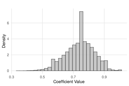
Figure 1: Density of the coefficient values in matrix $G$

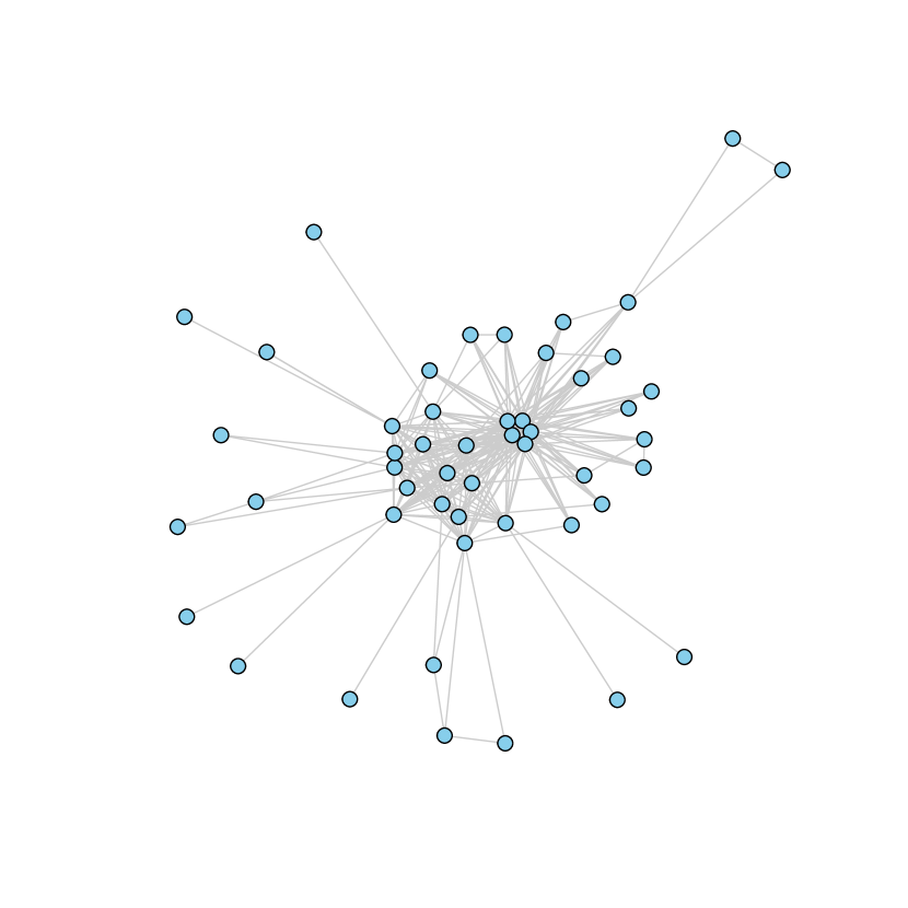
(a) $H^{5\%}$

(b) $H^{10\%}$

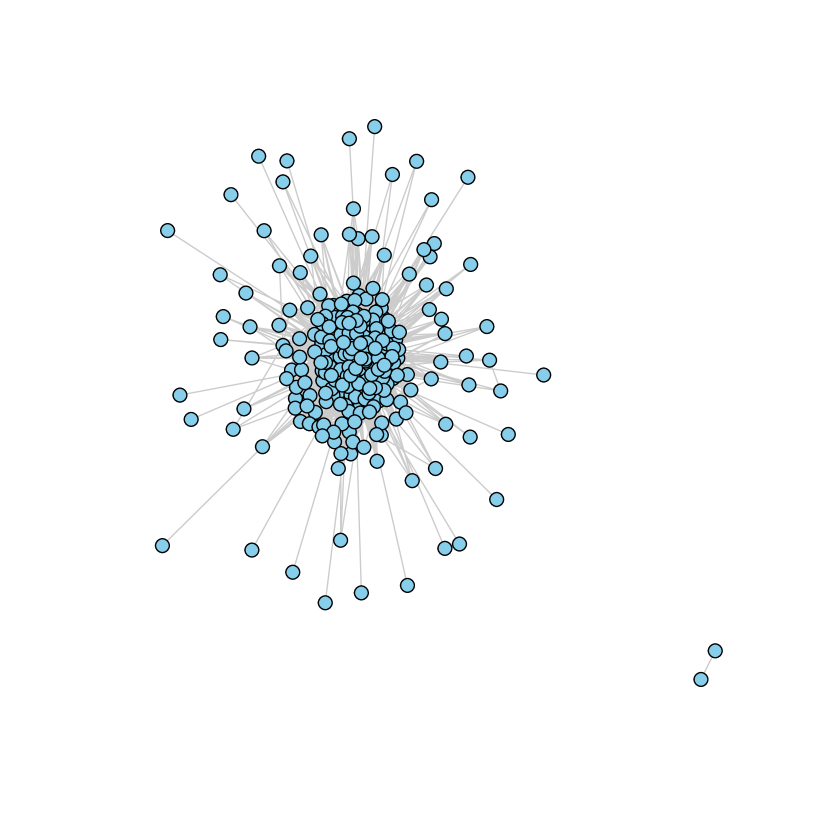
(c) $H^{15\%}$

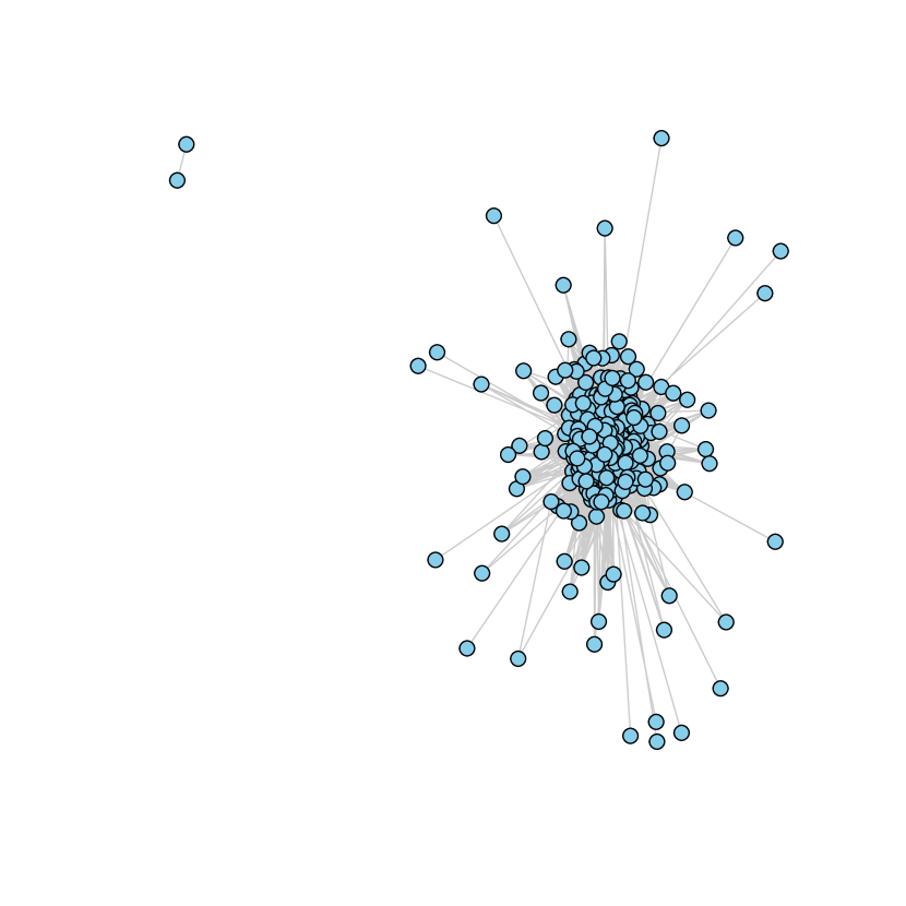
(d) $H^{20\%}$

Figure 2: Density of the coefficient values in matrix $G$

The density plot of the coefficient values in the similarity matrix $G$ is represented in Figure 1. The density function looks close to a Gaussian, with a mean coefficient at $74\%$, and a standard deviation of about $1\%$. This tight distribution indicates a high level of consistency across households in the data. Figure 2 plots the networks $H^{\alpha}$, for $\alpha\in\{5\%,10\%,15\%,20\%\}$, excluding isolated nodes, and reveals a striking result: irrespective of $\alpha$, the networks consistently feature a single dominant component. This indicates that, despite differences in decision patterns, households share sufficient overlap in their revealed preferences to form a cohesive network structure. For $\alpha=20\%$, we find that 90% households are connected in the main component. This indicates that, despite differences in decision patterns, households share sufficient overlap in their revealed preferences to form a cohesive network structure.This finding reinforces the results of Crawford and Pendakur (2012), who used a minimum partitioning approach to identify four to five distinct consumption types in a sample of 500 observations. In their analysis, 2/3 of observations were classified into a single type, with two types explaining 85% of the data. By adopting a permutation-based approach, we uncover a more nuanced and interconnected structure. Although households might appear incompatible under a strict partitioning scheme, they still form a cohesive network rather than disjoint clusters.

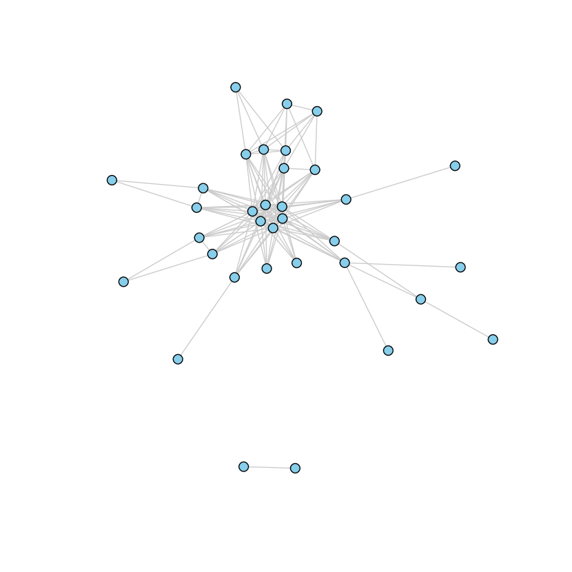
(a) $H^{5\%}$

(b) $H^{10\%}$

(c) $H^{15\%}$

(d) $H^{20\%}$

Figure 3: Density of the coefficient values in matrix $G_{\min}$

Additionally, we observe a substantial number of isolated households in networks $H^{\alpha}$, especially for $\alpha\in\{5\%,10\%\}$. This divergence does not appear to result from our partitioning algorithm, which might over-fragment types. To investigate further, we recomputed the networks $H^{\alpha}$ for $\alpha\in\{5\%,10\%,15\%,20\%\}$ on a subsample of 100 households using the minimum partitioning approach outlined in Section 3, rather than the partitioning approach of Procedure 1. The resulting networks, represented in Figure 3, also feature a single dominant component.

The previous result that households belong to one cohesive cluster does not mean that there are no heterogeneity patterns. To gain further insight into the structure of unobserved heterogeneity, we report in Table 3 standard network metrics that summarize distinct aspects of the heterogeneity structure captured by the adjacency matrices $H^{\alpha}$, for $\alpha\in\{5\%,10\%,15\%,20\%\}$. The number of edges increases significantly as the threshold becomes more permissive—from 286 edges at $\alpha=5\%$ to 24,525 edges at $\alpha=20\%$. The average degree metric provides additional insight into the network’s density. At $\alpha=5\%$, the average degree is only 1.43, indicating that households are sparsely connected, with each household linking to just over one other household on average. As $\alpha$ increases, the average degree rises to 122.62 at $\alpha=20\%$, suggesting that many households become densely interconnected at higher similarity thresholds. The clustering coefficient measures the extent to which households form tightly knit subgroups. Interestingly, we find that the clustering coefficient remains relatively high across all thresholds, ranging between 0.55 and 0.71. This indicates a strong tendency for households with similar preferences to form local clusters, even as the network becomes denser. The average path length, which measures the number of steps required to traverse the largest component of the network, provides insight into the network’s reachability. We find that the average path length remains stable across all thresholds, varying between 1.70 and 2.13.

Setting an appropriate precision threshold $\alpha$ in the analysis of heterogeneity presents a key challenge. If $\alpha$ is set too low, the resulting network $H^{\alpha}$ may have very few connections, yielding a sparse and relatively uninformative similarity structure. Conversely, if $\alpha$ is set too high, the network risks becoming overly dense, with most households connected to each other, thereby obscuring meaningful clusters of behavioral similarity. The choice of $\alpha$ thus requires balancing sparsity and connectivity to ensure that the network captures relevant patterns of heterogeneity without becoming either too fragmented or too saturated. In the analysis that follows, we present results for two key thresholds: a stringent threshold of $\alpha=5\%$, where households must be highly compatible to be linked, and a more permissive threshold of $\alpha=10\%$, where the network remains well-connected but avoids overwhelming density.

4.2 Observed Heterogeneity: Main Results

We implemented the permutation approach of Section 2.4 to evaluate the informativeness of all the observable characteristics of Table 2 on the similarity within the networks $H^{\alpha}$, for $\alpha\in\{5\%,10\%\}$. Practically, for each observable characteristic $Z$, we built $N=1000$ synthetic dataset by randomly shuffling observable $Z$ across nodes in network $H^{\alpha}$, and implemented Procedure 3 for each metric $M(Z)\in\{R(Z),C(Z),H(Z),D(Z)\}$. In this procedure, we evaluate whether the observable $Z$ is or is not randomly assigned across the network $H^{\alpha}$, comparing the metric $M(Z)$ to the value of that metric in the network where observable $Z$ is randomly assigned. For each observable, we also quantified the deviation from randomness, computing the effect size for each metric, as outlined in Section 2.5.

Table 4 reports the standardized effect sizes, as defined in Equation (3), for the observable characteristics across four metrics — Pairwise similarity, Community Detection, Entropy, and Degree Centrality —and for two network precision levels, $\alpha=5\%$, and $\alpha=10\%$. Each coefficient in the table measures how many standard deviations the observed metric deviates from its expected value under a null scenario in which the observable is randomly assigned to nodes. Positive and significant coefficients indicate that the corresponding observable characteristic is strongly and systematically associated with the network’s heterogeneity structure, from Procedure 3.

Pairwise Similarity: This metric captures how frequently nodes sharing a particular characteristic are directly connected. Results show that older households, and households with small family sizes are notably more likely to be connected to each other compared to what would be expected under random assignment. For instance, households with small family sizes display effect sizes ranging from 4.9 to 5.7 standard deviations above the null benchmark—an effect that is robust across both $\alpha=5\%$, and $\alpha=10\%$ and statistically significant at the 1% level. Old-age households similarly exhibit significant positive deviations, on the order of 2.3 to 3.2 standard deviations, indicating that they also form disproportionately more direct links within the network than if the old age labels were randomly permuted. These findings suggest that households defined by these particular attributes (low family size and old age) cluster together at the most immediate, local level of network structure.

Community Detection: Turning to the community detection metric, which evaluates alignment at a larger structural scale, we again find a strong and statistically significant association for low family size, and old age. Households with these characteristics are not just forming local links; they also tend to be grouped into the same communities.

Entropy: The Entropy metric provides insights into how observables are distributed across the identified communities. The Entropy measure reveals that some characteristics are linked to significantly higher entropy. Households with intermediate and large sizes as well as younger households tend to span diverse communities identified in the similarity networks. This suggests that young age as well as medium to large family size households are able to adopt more diverse consumption patterns than what would be predicted under random assignment.

Degree Centrality: The Degree Centrality metric shifts the focus to the positional prominence of certain types of households within the network. Our results indicate that younger, and medium to large family-size households occupy more central positions—interpreted as having more connections relative to the null scenario. While these attributes may not create as tightly knit communities or strongly predictable links as old age or low family size households do, they appear to be “key players” in the network’s connectivity, as households with these characteristics link various parts of the network. This finding suggests a more adaptive or versatile consumption behavior among these groups, allowing them to connect more broadly and fluidly within the heterogeneity structure identified by the similarity network.

Overall, our analysis uncovers a nuanced relationship between observable characteristics and the network’s revealed preference heterogeneity. Some variables, like low family size, and old age strongly align with the network structure at both local (edges) and global (communities) levels. Other observables—such as young age, and medium/large family size—become relevant when considering entropy or centrality measures. These distinctions underscore that “heterogeneity” can be interpreted through multiple lenses—ranging from immediate connections to community membership and network position—each reflecting a different facet of how observable attributes map onto underlying preference structures.

4.3 Seasonality

A potential concern is that household consumption patterns may vary systematically across seasons, reflecting changes in needs, availability of goods, or other seasonal factors. To explore seasonal fluctuations in preferences, we constructed a seasonally disaggregated dataset as follows. From an initial subset of 100 households, we divided each household $i$ into four “season-households” $(i(\text{summer}),i(\text{autumn}),i(\text{winter}),i(\text{spring}))$, each representing that household’s consumption choices during a particular season. Because our dataset tracks households over two years, each season-household is represented by approximately six observations. This procedure yields a total of 400 season-households.

We applied the same similarity-network construction methods to this seasonally disaggregated dataset. This approach allows us to test if a given household $i$ remains consistently linked to itself across different seasons, and whether seasonal labels act as meaningful predictors of the network’s heterogeneity structure. In other words, does the observed heterogeneity primarily stem from underlying household-level differences, or can seasonal variations also explain a significant portion of the network links?

Table 5 presents the results for the seasonal dataset. The table reports the effect sizes (3) for the household and season indicators on three measures— Pairwise similarity, Community Detection, and Entropy—evaluated at two network precision levels $\alpha=5\%$ and $\alpha=10\%$. The results clearly indicate that the household dimension is a strong and stable predictor of heterogeneity. Specifically, the household indicator exhibits large, positive, and highly significant coefficients in both the Ratio and Community Detection metrics. This implies that each household’s seasonal manifestations remain closely connected to one another, reinforcing the notion of stable underlying preferences that transcend seasonal shifts. Only the spring seasonal indicator shows a modest statistically significant effect on the network structure through the Community Detection and Entropy metrics. Taken together, these findings suggest that households do exhibit consistent consumption patterns across seasons, and seasonal factors - except spring - are not driving the observed heterogeneity in the network $H^{\alpha}$. While events like Easter might create some uniformity in consumption behavior during spring, it remains unclear why an effect, albeit modest, is only present for spring and not for other seasons.

4.4 Further Considerations on the Stability of Household Preferences

In principle, different decision models could govern a household’s choices over time, independent of seasonal patterns or other directly observable factors. Such variability might stem from changes in bargaining power within the household, evolving needs, or even occasional data errors or misrecorded choices. To explore these possibilities, we extend our analysis by allowing for multiple decision models within each household.

Identifying Multiple Decision Models Within a Household

For each household $i$, we partition the set of observed decisions into subsets, such that each subset independently satisfies the revealed preference (RP) conditions of Definition 2. We use the partitioning approach of Proposition 1, although it is also possible to use a minimum partitioning approach within households. The choice of partitioning strategy might not have an effect on the analysis, as both partitioning strategies may give similar outcomes when there are at most two types according to the approach of Proposition 1. As shown next, this is the case for 195 out of the 200 households.

Our overall procedure can be interpreted in several ways. Drawing on Cherchye, de Rock and Vermeulen (2007); Cherchye, De Rock and Vermeulen (2009), one may view each type within a given household as representing a different “situation-dependent dictator”, i.e., a particular household member fully responsible for certain choices. Alternatively, it may reflect changing needs over time (e.g., a household adapting as a newborn grows into a toddler) or simply data noise and errors that artificially create the appearance of multiple decision models.

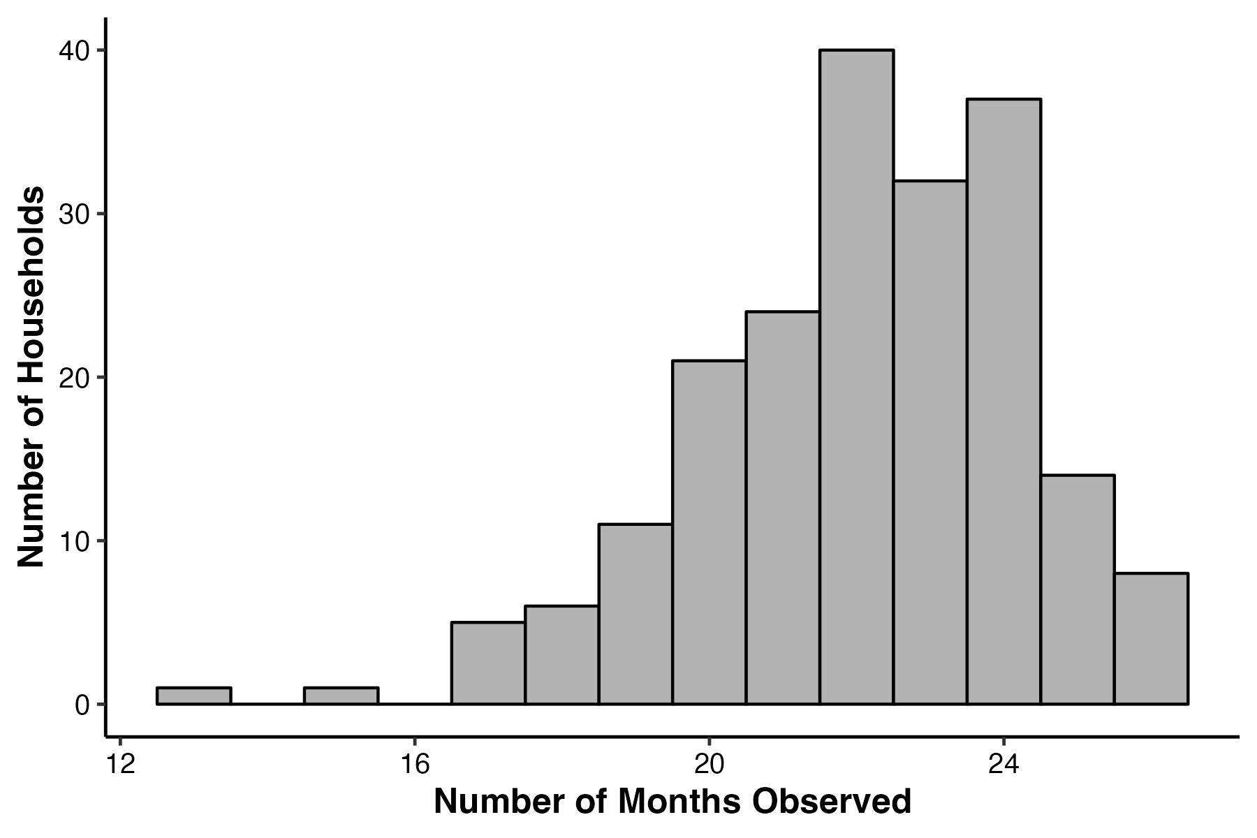
Figure 5: Number of Observations per “Main” Type

After applying this procedure to a subset of 200 households, we end up with a larger sample of 372 “household-types.” Each type-household corresponds to a coherent subset of the original household’s decisions that is internally rational (in the GARP₁ sense). Figure 4 illustrates the distribution of the number of types per household. No household requires more than three decision models to explain its choices. Specifically, 81% of households are best described by two distinct decision models, 16.5% have only one model, and 2.5% require three. Figure 5 shows the size of the main (majority) type for each household. The imbalance uncovered in Figure 5 raises questions about whether secondary types represent meaningful decision models or are merely statistical artifacts. While it is possible to complement the analysis by an approximate rationality test for secondary types, this test would inherently be conservative, since it is hard to falsify random behavior in consumer data with only few observations.

Permutation Approach to “Household-Types” Disaggregated Data

We applied the same similarity-network construction methods to the type-households disaggregated dataset, allowing us to study the structure and coherence of these type-households within and across households. While, by construction, two types within the same household might hardly be linked in a similarity network, they can belong to similar communities or exhibit indirect links via shared connections to other households. This provides a way to examine whether types within the same household are systematically related, especially in broader network terms through the community detection or entropy metrics.

The results of the analysis are reported in Table 6. The Household variable—indicating whether two types originate from the same household—shows significantly higher similarity in both the Pairwise Similarity (Column (2)) and Community Detection (Columns (3),(4)) metrics, implying that multiple types within a single household are more closely connected than expected under random assignment. It is not surprising that two types within a households are not directly connected at the $\alpha=5\%$ level, from Column (1), since types within a household are, by construction, not consistent in the GARP₁ sense. Additionally, new patterns emerge regarding education, and income. These patterns are hard to interpret, since they might be an artifact implied by dis-aggregating households into types. Indeed, since types within household are close and share household-level characteristics such as education, income, or family size, then we might over-estimate the predictive power of these household-level characteristics in Table 6.

Minimum Partition Approach

Finally, we applied the minimum partition approach of Section 3 in a subsample of 100 households and constructed the corresponding similarity network. This exercise allows us to assess whether the choice of partitioning procedure meaningfully influences how observable characteristics align with the network’s heterogeneity structure. When implementing the minimum partitioning algorithm (4), we put a time limit of 1 second, so that synthetic datasets where the algorithm takes more than 1 second to find all cycles are not considered when computing the similarity network. Only 3 synthetic data were disregarded for that reason. In what follows, we denote $G_{\min}$ the similarity network that we obtained using the minimum partitioning algorithm in our permutation approach, and $G$ the similarity network that we obtained with our main partitioning approach in the same subsample of 100 households.

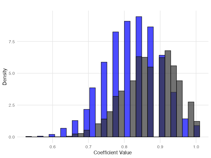
Figure 6: Density of the coefficient values in $G$ and $G_{\min}$

To compare the two similarity networks, we first represented in Figure 6 the density function of the empirical distribution of the coefficient values in the similarity matrices $G$ and $G_{\min}$. Both empirical distributions are single-peaked, but the coefficient values derived from our partitioning approach using Procedure 1 are, on average, higher (mean = 0.87) compared to the minimum partitioning approach (mean = 0.82).

We implemented the permutation approach of Section 2.4 to evaluate the informativeness of observable characteristics on the similarity within the networks $H^{5\%}$, recovered using both partitioning strategies. Table 7 reports the resulting standardized effect sizes across the network metrics under both the minimum partitioning approach (columns (1), (3), (5), (7)) and our partitioning approach of Section 2.2 (the remaining columns). Overall, both methods lead to broadly consistent findings. Old households are significantly more connected according to the Pairwise Alignment metric, with effect sizes of 3.662 under the Minimum Partitioning approach versus 3.618 under Procedure 1, both significant at the 1% level. Similarly, Young households have a significantly higher degree centrality in $H^{5\%}$ according to both approaches. Again, both the magnitude and significance level are comparable. These two results echo the patterns found in the main sample presented in Table 4.

Finally, there are additional results that arise in the smaller sample. We find that low-income households are significantly more connected according to the Pairwise Alignment metric, with effect sizes of 1.474 under the Minimum Partitioning versus 1.540 under Procedure 1, both significant at the 10% level. Some smaller differences emerge, however. Under Procedure 1, low family size appears highly predictive in the Pairwise Alignment metric - consistent with Table 4 - while this relationship is not significant in the Minimum Partitioning approach. Conversely, the Minimum Partitioning approach reveals that low-income also plays a significant role in shaping heterogeneity as measured by the Community Detection metric, whereas this finding does not hold under Procedure 1. Despite these nuances, both partitioning strategies yield broadly similar insights regarding which characteristics drive similarity or heterogeneity in the consumption networks. Because Procedure 1 is less computationally intensive than the Minimum Partitioning approach, it likely remains the more practical choice for permutation-based analyses on larger datasets.

5 Conclusion

In this paper, we introduced a novel network-based methodology to capture unobserved heterogeneity in consumer behavior, building upon the partitioning framework of Crawford and Pendakur (2012). Unlike traditional approaches that pool all of an agent’s choices into a single type, our permutation-based method repeatedly samples a subset of choices from each agent and partitions them into GARP-consistent groups using Mixed Integer Linear Programming (MILP). This iterative process generates a probabilistic similarity matrix $G$, where each entry $G_{i,j}$ represents the fraction of synthetic datasets in which agents $i$ and $j$ share the same type. By applying thresholding rules, we derive adjacency matrices $H^{\alpha}$ for various precision levels $\alpha$, effectively mapping the unobserved heterogeneity in consumer microdata into networks.

We bridged the gap between unobserved and observable heterogeneity by implementing a permutation test that assesses how well observable characteristics explain the similarity patterns in the networks characterizing the unobserved heterogeneity. By computing standardized effect sizes for various network metrics—pairwise similarity, community detection, entropy, and degree centrality—we quantified the extent to which each observable variable (such as family size and income) influences the network structure. This non-parametric approach allows us to measure the impact of observables without relying on predefined functional forms, offering a flexible and robust framework for understanding heterogeneity.

We applied our method to the Stanford Basket Dataset, encompassing 400 households and over 57,000 transactions across 368 product categories over 26 months. We found that networks $H^{\alpha}$, for $\alpha\in\{5\%,10\%,15\%,20\%\}$ consistently feature a single dominant component. Hence, despite differences in decision patterns, households share sufficient overlap in their revealed preferences to form a cohesive network structure. This finding aligns with and extends the results of Crawford and Pendakur (2012), who identified a handful of distinct consumption types under a strict partitioning framework. Our analysis reveals that even households classified as incompatible under strict partitioning still exhibit enough similarity to form an interconnected network rather than disjoint clusters, suggesting that consumer heterogeneity operates on a more interconnected continuum than previously understood.

Building on the networks’ structures, we further investigated how observable characteristics shape consumer heterogeneity and the structure of $H^{\alpha}$, for $\alpha\in\{5\%,10\%\}$. Our analysis revealed significant clustering based on family size and age. Specifically, small and old households formed tightly knit subgroups, exhibiting effect sizes between 2.2 and 5.7 standard deviations above the null benchmark in pairwise similarity and community detection metrics. Additionally, young and medium to large family households emerged as central agents within the network, bridging diverse consumption patterns. These findings highlight the nuanced ways in which observable characteristics shape consumer heterogeneity, demonstrating that certain demographics not only cluster together but also play pivotal roles in connecting various consumer segments.

We further extended our methodology to address additional dimensions of heterogeneity. By incorporating seasonality, we demonstrated that household preferences remain stable across different seasons, as evidenced by consistently significant household-level clustering. Additionally, by partitioning households into multiple decision-making types, we uncovered that types within the same household are significantly more connected. Finally, we compared our main partitioning approach with the minimum partitioning strategy. Both methods ultimately yield consistent insights into the structure of heterogeneity.

Our approach presents certain limitations. The partitioning algorithms are computationally intensive, which may hinder scalability. Additionally, our analysis focused on partitioning based on GARP conditions. Future research should explore the application of our framework using alternative revealed preference conditions beyond GARP, such as collective rationality, habit formation, or intertemporal choice models. These extensions could enhance the versatility of our methodology and provide deeper insights into different dimensions of individual behavior and heterogeneity.

Tables

	A	B	C
Decision 1	$x$	$z$	$w$
Decision 2	$y$	$z$	$w$

Table 1: Example illustrating the permutation approach for three agents ($A$, $B$, and $C$) making two decisions each.

Variable	Number of Households
Family Size
Low	183
Mid	164
Large	53
Income
Low	108
Mid	170
High	122
Age
Young	106
Mid	174
Old	120
Education
Primary Education	22
High School	166
College	212
Observations	400

• Middle-aged households are defined as those in which the average age of the spouses is between 30 and 65 years. Old-aged households have an average age of spouses exceeding 65 years. For households with both spouses present, the reported education level reflects the average education of both spouses. Mid-size households consist of 3 to 4 members, while large households have more than 4 members. The low-income category includes households with an annual income below $20,000; the middle-income category covers those with an income between $20,000 and $45,000; and the high-income category includes households with an income above $45,000.

Table 2: Sociodemographic Variables

$\alpha$	Nodes	Edges	Avg. Degree	Isolated Nodes	Clustering Coeff.	Avg. Path Length
0.05	400	286	1.43	350	0.65	2.09
0.10	400	3051	15.26	206	0.55	2.13
0.15	400	8614	43.07	113	0.60	1.96
0.20	400	24525	122.62	36	0.71	1.70

• Note: The table reports key characteristics of the similarity networks $H^{\alpha}$ for $\alpha\in\{5\%,10\%,15\%,20\%\}$. Nodes refer to households in the dataset. Edges represent connections between households that meet the threshold criterion $\alpha$. Average Degree is the average number of connections per household. Isolated Nodes are households with no connections. The Clustering Coefficient measures the likelihood that two connected nodes also share a connection with a third node, indicating the tendency to form tightly knit groups. The Average Path Length is the average number of steps along the shortest paths between all pairs of nodes, describing how efficiently information or influence propagates in the network.

Table 3: Network $H^{\alpha}$ Characteristics for $\alpha\in\{5\%,10\%,15\%,20\%\}$

Table 4: Heterogeneity explained by Observable Characteristics

	Paiwise Alignment		Comm. Detec.		Deg. Cent.		Entropy
	$R(Z)$		$C(Z)$		$D(Z)$		$H(Z)$
	(1)	(2)	(3)	(4)	(5)	(6)	(7)	(8)
Family Size
Low	5.683***	4.908***	2.046*	1.429*	-2.719	-3.002	-2.725	-1.617
Mid	-0.381	-1.028	-0.992	-0.929	1.47*	1.166	1.221*	1.421*
Large	-1.574	-2.335	-1.474	-3.253	1.839**	2.665***	1.633**	2.848***
Income
Low	-1.004	-0.615	0.079	1.28	1.355	0.452	-0.557	-1.897
Mid	-0.046	-0.724	-0.82	-1.143	-0.819	0.082	1.047	0.495
High	0.361	0.49	1.258	-0.981	-0.552	-0.596	-0.878	0.741
Age
Young	-1.281	-2.287	-1.288	-1.963	1.767**	3.049***	0.693	2.049**
Mid	-0.311	0.712	-0.523	0.333	0.151	-0.45	-0.843	0.563
Old	2.281**	3.202***	2.872**	2.05**	-1.92	-2.502	-3.375	-3.04
Education
Primary	0.6885	-0.0467	-	-	-	-	-0.898	-0.072
HS	-1.549	-0.242	-0.326	-0.308	0.937	0.027	-0.859	-0.197
College	-1.274	-0.474	-0.428	-0.181	-0.480	0.230	0.689	-0.214
$\alpha$
$5\%$	Y	N	Y	N	Y	N	Y	N
$10\%$	N	Y	N	Y	N	Y	N	Y

• Note: The estimation procedure involves three main steps. Step 1: 50 synthetic datasets were generated by randomly sampling one consumption vector for each household from the observed 26 periods. Step 2: we generated similarity matrices by applying Procedure 1 to partition the households into types in each synthetic dataset. We used a precision threshold of 0.95, and generated similarity matrices at levels $\alpha=0.05$ and $\alpha=0.10$. Step 3: for each observable characteristic $Z$ in Table 2, we generated a set of $1000$ randomized networks by shuffling $Z$ across nodes. We then applied Procedure 3 to test whether observable $Z$ is not randomly assigned in the similarity network $H^{\alpha}$. The reported coefficients are normalized effect sizes derived using Equation (3), where higher values indicate stronger alignment of the observable with the heterogeneity structure relative to the null distribution. Significance levels are from the statistical test of Procedure 3, and are denoted by * ($p<0.1$), ** ($p<0.05$), and *** ($p<0.01$). Rows $\alpha=5\%$, and $\alpha=10\%$ indicate the significance thresholds used to construct the similarity network $H^{\alpha}$. The Community Detection and Degree Centrality metrics cannot be computed for the Primary Education variable, as the 22 households with that education level are isolated in networks $H^{\alpha}$, $\alpha\in\{5\%,10\%\}$.

Table 5: Seasonability Effect

	Pairwise Alignment		Comm. Detec.		Entropy
	$R(Z)$		$C(Z)$		$H(Z)$
	(1)	(2)	(3)	(4)	(5)	(6)
Household	3.941***	4.828***	3.688***	2.796***	-3.185	-2.178
Season
Summer	0.368	1.045	0.019	0.265	0.045	-1.117
Autumn	-0.736	-0.849	-1.234	0.272	1.229	0.063
Winter	-0.816	-0.568	-0.876	0.753	0.926	-0.686
Spring	1.051	0.128	2.267**	-1.294	-2.645	1.393*
$\alpha$
$5\%$	Y	N	Y	N	Y	N
$10\%$	N	Y	N	Y	N	Y

• Note: The data used to generate the similarity matrices are from a subsample of 100 households. Each household is then divided into four “season-household”. Reported coefficients are normalized effect sizes derived using Equation (3), where higher values indicate stronger alignment of the observable with the heterogeneity structure relative to the null distribution. Significance levels are from the Statistical Test of Section 2.4, and are denoted by * ($p<0.1$), ** ($p<0.05$), and *** ($p<0.01$). Rows $\alpha=5\%$ and $\alpha=10\%$ indicate the significance thresholds used to construct the similarity network $H^{\alpha}$.

Table 6: Heterogeneity Explained in “Household-type” Disaggregated Data

	Pairwise Alignment		Comm. Detec.		Deg. Cent.		Entropy
	$R(Z)$		$C(Z)$		$D(Z)$		$H(Z)$
	(1)	(2)	(3)	(4)	(5)	(6)	(7)	(8)
Household	2.409	2.882***	1.867**	1.409*	-0.167	-0.745	-2.187	0.609
Family Size
Low	-1.215	-0.275	0.567	-0.704	-0.313	-0.849	-0.131	-0.183
Mid	-1.745	-1.253	-1.220	-0.600	0.545	0.956	1.368*	-0.481
Large	0.079	0.132	-0.846	0.559	-0.423	-0.200	1.302*	-0.525
Income
Low	1.760*	2.585**	3.744***	2.255**	-0.837	-1.987	-2.056	-1.263
Mid	0.403	-0.795	-0.428	-1.012	1.233	1.422*	-0.237	0.222
High	0.602	-0.867	-1.093	-1.205	-0.495	0.542	0.268	0.804
Age
Young	0.267	-0.249	-0.866	-0.344	-0.242	0.149	0.427	-0.057
Mid	-1.676	-1.078	-1.210	-1.972	0.006	1.295	1.621**	1.389*
Old	-0.082	1.587*	0.605	1.386*	0.184	-1.395	-1.944	-1.867
Education
Primary	2.753**	2.550***	-	-	2.473***	2.397**	-1.417	0.411
HS	0.509	-0.797	-0.528	-0.233	2.481***	2.393**	-0.200	-0.613
College	0.719	-0.475	0.310	-0.897	1.930**	1.362*	-0.059	-0.134
$\alpha$
$5\%$	Y	N	Y	N	Y	N	Y	N
$10\%$	N	Y	N	Y	N	Y	N	Y

• Note: The data used to generate the similarity matrices are from a subsample of 200 households. Each household is partitioned into “types” using Procedure 1. The reported coefficients are normalized effect sizes derived using Equation (3), where higher values indicate stronger alignment of the observable with the heterogeneity structure relative to the null distribution. Significance levels are from the statistical test of Procedure 3, and are denoted by * ($p<0.1$), ** ($p<0.05$), and *** ($p<0.01$). Rows $\alpha=5\%$, and $\alpha=10\%$ indicate the significance thresholds used to construct the similarity network $H^{\alpha}$. The Community Detection and Degree Centrality metrics cannot be computed for the Primary Education variable, as the 22 households with that education level are isolated in networks $H^{\alpha}$, $\alpha\in\{5\%,10\%\}$.

Table 7: Comparison: Minimum Partitioning vs Procedure 1

	Pairwise Alignment		Comm. Detec.		Deg. Cent.		Entropy
	$R(Z)$		$C(Z)$		$D(Z)$		$H(Z)$
	(1)	(2)	(3)	(4)	(5)	(6)	(7)	(8)
Family Size
Low	0.392	3.079***	-0.551	1.234	-1.749	-2.713	0.562	-0.362
Med	-1.455	-0.846	0.523	-0.960	1.024	1.103	0.921	0.885
Large	-0.982	-2.157	-0.249	-1.455	0.934	2.175**	0.627	1.492*
Income
Low	1.474*	1.54*	2.317**	1.163	-1.355	-1.383	-1.588	-2.906
Mid	-1.316	-0.488	-0.691	0.587	1.885**	0.327	0.378	-0.044
High	0.374	-0.829	1.136	-1.001	-0.502	1.043	-1.347	0.629
Age
Young	-2.318	-3.629	-0.634	-1.580	2.536***	3.838***	-0.353	0.328
Mid	-0.625	0.298	-1.180	-1.192	0.617	-0.686	0.665	1.052
Old	3.662***	3.618***	1.246	2.734**	-2.723	-2.764	-2.333	-3.408
Education
HS	1.104	1.635*	0.548	1.215	-1.007	-2.069	-2.402	-1.311
College	0.871	0.800	2.604**	-0.146	1.294	2.662***	-2.902	-1.582
Primary	-0.956	-1.997	-	-	-	-	-	-
Partitioning Procedure
Minimum	Y	N	Y	N	Y	N	Y	N
Procedure 1	N	Y	N	Y	N	Y	N	Y

• Note: The data used to generate the similarity matrices are from a subsample of 100 households. The reported coefficients are normalized effect sizes derived using Equation (3), where higher values indicate stronger alignment of the observable with the heterogeneity structure relative to the null distribution. The effect sizes are computed relative to the similarity matrix $H^{5\%}$. Significance levels are from the statistical test of Procedure 3, and are denoted by * ($p<0.1$), ** ($p<0.05$), and *** ($p<0.01$). The Community Detection and Degree Centrality metrics cannot be computed for the Primary Education variable, as the 22 households with that education level are isolated in networks $H^{\alpha}$, $\alpha\in\{5\%,10\%\}$.

Figures

Note: This figure represents the empirical distribution of the coefficients in matrix $G$. To generate $G$ we proceeded in two steps. First, 50 synthetic datasets were generated by randomly sampling one consumption vector for each household from the observed 26 periods. Second, we applied Procedure 1 to partition the households into types in each synthetic dataset.

Note: The figures represent the similarity network $H^{\alpha}$, excluding isolated nodes, for $\alpha\in\{5\%,10\%,15\%,20\%\}$. $H^{\alpha}(i,j)=1$ if $G(i,j)\geq 1-\alpha$, $H^{\alpha}(i,j)=0$ otherwise for any pair of households $i,j\in\mathcal{I}$. To generate matrix $G$, we proceeded in two steps. First, 50 synthetic datasets were generated by randomly sampling one consumption vector for each household from the observed 26 periods. Second, we applied Procedure 1 to partition the households into types in each synthetic dataset.

Note: The figures represent the similarity network $H^{\alpha}$, excluding isolated nodes, for $\alpha\in\{5\%,10\%,15\%,20\%\}$. $H^{\alpha}(i,j)=1$ if $G(i,j)\geq 1-\alpha$, $H^{\alpha}(i,j)=0$ otherwise for any pair of households $i,j\in\mathcal{I}$. To generate matrix $G_{\min}$, we proceeded in two steps. First, 50 synthetic datasets were generated by randomly sampling one consumption vector for each household from the observed 26 periods. Second, we applied the minimum partitioning approach of Section 3 to partition the households into types in each synthetic dataset.

Figure 4: Number of Types per Household

Note: This figure represents the empirical distribution of the number of types per household. For each household, the number of types is computed using a minimum-partitioning algorithm similar to (4), as discussed in Section 4.4.

Note: This figure represents the empirical distribution of the number of months or observations that belong to the main type for each household. The main type in a given household is the type with the highest share of observations. Each household is partitioned into GARP₁ consistent types using a minimum partitioning algorithm.

Note: We used 100 consumers to generate the $G$ and $G_{\min}$ matrices. The minimum partitioning approach of Section 3 was used to build $G_{\min}$, and our main partitioning approach of Procedure 1 was used to build $G$. When implementing the minimum partitioning algorithm (4), we put a time limit of 1 second, so that synthetic datasets where the algorithm takes more than a one second to find all GARP violating cycles are not considered when computing matrix $G_{\min}$. Only 3 out of 50 synthetic data were excluded for that reason.

Appendix

A.1 Proof of Proposition 1

Inequality (IP 1) guarantees that $\psi^{n,k}=0$ implies that $U^{k}>U^{n}$. Inequality (IP 2) guarantees that $\psi^{n,k}=1$ implies that $U^{n}\geq U^{k}$. Additionally, from inequality (IP 3), if $x_{i(n)}e^{n}p^{n}.q^{n}\geq p^{n}.q^{k}$, then $U^{n}\geq U^{k}$. Indeed, if $x_{i(n)}e^{n}p^{n}.q^{n}\geq p^{n}.q^{k}$, then $\psi^{n,k}=1$ necessarily, as otherwise (IP 3) would create the contradiction

$$0\leq x_{i(n)}e^{n}p^{n}q^{n}-p^{n}q^{k}<0,$$

and from (IP 2), $\psi^{n,k}=1$ implies that $U^{n}\geq U^{k}$. Hence, $x_{i(n)}e^{n}p^{n}.q^{n}\geq p^{n}.q^{k}$ implies $U^{n}\geq U^{k}$. Applying a similar reasoning to (IP 1) and (IP 4), we find that $x_{i(k)}e^{k}p^{k}.q^{k}>p^{k}q^{n}$ implies $U^{k}>U^{n}$. Hence, we have demonstrated the following Corollary:

Corollary 1.

Inequalities (IP 1) - (IP 4) guarantee that

$$x_{i(n)}e^{n}p^{n}.q^{n}\geq p^{n}q^{k}\text{ implies }U^{n}\geq U^{k}$$ (GARP 1)

$$x_{i(k)}e^{k}p^{k}.q^{k}>p^{k}.q^{n}\text{ implies }U^{k}>U^{n}$$ (GARP 2)

From a direct extension of Theorem 2 in Demuynck and Rehbeck (2023), the four inequalities (IP 1) - (IP 4) guarantee that the GARP_xe conditions of Definition 2 are satisfied with $xe=\{x_{i(n)}e^{n}\}_{n\in\mathcal{N}}$. Reciprocally, it is possible to show that conditions (GARP 1) and (GARP 2) imply that inequalities (IP 1) - (IP 4) are satisfied. The proof closely follows the proof of Corollary 1 in Demuynck and Rehbeck (2023), and is omitted. Thus, the aggregate data satisfy GARP_xe if and only if inequalities (IP 1) - (IP 4) are satisfied, thus concluding the proof that the $LS(e)$ set can be computed using the mixed integer linear programming constraints.

References

- (1)
- Afriat (1967) Afriat, S. N. 1967. “The Construction of Utility Functions from Expenditure Data.” International Economic Review 8(1):67–77.
- Aguiar and Kashaev (2020) Aguiar, Victor H and Nail Kashaev. 2020. “Stochastic Revealed Preferences with Measurement Error.” The Review of Economic Studies 88(4):2042–2093.
- Bar-Shira (1992) Bar-Shira, Ziv. 1992. “Nonparametric Test of the Expected Utility Hypothesis.” American Journal of Agricultural Economics 74(3):523–533.
- Bell and Lattin (1998) Bell, David R. and James M. Lattin. 1998. “Shopping Behavior and Consumer Preference for Store Price Format: Why ”Large Basket” Shoppers Prefer EDLP.” Marketing Science 17(1):66–88.
- Blow, Browning and Crawford (2008) Blow, Laura, Martin Browning and Ian Crawford. 2008. “Revealed Preference Analysis of Characteristics Models.” The Review of Economic Studies 75(2):371–389.
- Browning (1989) Browning, Martin. 1989. “A Nonparametric Test of the Life-Cycle Rational Expections Hypothesis.” International Economic Review 30(4):979–992.
- Cherchye, de Rock and Vermeulen (2007) Cherchye, Laurens, Bram de Rock and Frederic Vermeulen. 2007. “The Collective Model of Household Consumption: A Nonparametric Characterization.” Econometrica 75(2):553–574.
- Cherchye, De Rock and Vermeulen (2009) Cherchye, Laurens, Bram De Rock and Frederic Vermeulen. 2009. “Opening the Black Box of Intrahousehold Decision Making: Theory and Nonparametric Empirical Tests of General Collective Consumption Models.” Journal of Political Economy 117(6):1074–1104.
- Cherchye, Saelens and Tuncer (2024) Cherchye, Laurens, Dieter Saelens and Reha Tuncer. 2024. “From unobserved to observed preference heterogeneity: a revealed preference methodology.” Economica 91(363):996–1022.
- Cherchye et al. (2023) Cherchye, Laurens, Thomas Demuynck, Bram De Rock and Joshua Lanier. 2023. “Are Consumers (Approximately) Rational? Shifting the Burden of Proof.” The Review of Economics and Statistics pp. 1–45.
- Choi et al. (2007) Choi, Syngjoo, Raymond Fisman, Douglas Gale and Shachar Kariv. 2007. “Consistency and Heterogeneity of Individual Behavior under Uncertainty.” American Economic Review 97(5):1921–1938.
- Cosaert (2019) Cosaert, Sam. 2019. “What Types are There?” Computational Economics 53(2):533–554.
- Crawford (2010) Crawford, Ian. 2010. “Habits Revealed.” The Review of Economic Studies 77(4):1382–1402.
- Crawford and Pendakur (2012) Crawford, Ian and Krishna Pendakur. 2012. “How many types are there?” The Economic Journal 123(567):77–95.