Stochastic Optimal Control of Iron Condor Portfolios for Profitability and Risk Management
Abstract
Previous research on option strategies has primarily focused on their behavior near expiration, with limited attention to the transient value process of the portfolio. In this paper, we formulate Iron Condor portfolio optimization as a stochastic optimal control problem, examining the impact of the control process on the portfolio’s potential profitability and risk. By assuming the underlying price process as a bounded martingale within , we prove that the portfolio with a strike structure of has a submartingale value process, which results in the optimal stopping time aligning with the expiration date . Moreover, we construct a data generator based on the Rough Heston model to investigate general scenarios through simulation. The results show that asymmetric, left-biased Iron Condor portfolios with are optimal in SPX markets, balancing profitability and risk management. Deep out-of-the-money strategies improve profitability and success rates at the cost of introducing extreme losses, which can be alleviated by using an optimal stopping strategy. Except for the left-biased portfolios generally falls within the range of [50%,75%] of total duration. In addition, we validate these findings through case studies on the actual SPX market, covering bullish, sideways, and bearish market conditions.
keywords:
Iron Condor , Fractional Brownian Motion , Rough Heston , Optimal Stopping Time[label1]organization=School of Computer, Jiangsu University of Science and Technology, city=Zhenjiang, postcode=212003, state=Jiangsu Province, country=China \affiliation[label2]organization=Technical University of Munich, city=Munich, postcode=80333, state=Bavaria, country=Germany
1 Introduction
Option portfolio optimization can be formulated as a stochastic optimal control problem, where the portfolio value process indicated by is a state process, which can be partly controlled by some control process . For a given initial point , we consider as a controlled stochastic differential equations:
| (1) |
where and are some given functions with
| (2) |
where is a d-dimensional Wiener process. The control process is defined to be adapted to the , denoted by . Moreover, it is also an admissible function in the admissible control law classes for all and .
In real applications, the state process must reside within a fixed domain. Consider a general situation where all options in the portfolio share the same expiration date, . Moreover, let us assume a group of option strategies where the maximum potential loss and maximum potential gain are predetermined at the initial state . This setup naturally forms a domain for such a class of option portfolios, denoted as . When the state process reaches the boundary , the investment terminates. Thus, we define the stopping time as follows:
| (3) |
where .
Furthermore, we define the instantaneous utility function as and the terminal utility (or bequest) as , where . The optimization problem is then to maximize the following expected value:
| (4) |
A well-known option strategy belonging to the above class is the Iron Condor strategy Cohen (2005); Woodard (2011). Without loss of generality, only contains a underlying process and a bank account process as follows:
| (5) |
where is the short rate. From general portfolio theory process can be expressed as,
| (6) |
where is the weight of the underlying asset.
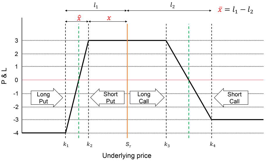
If we do not consider optimizing consumption and set , the utility function depends solely on the terminal wealth, which is the usual case for Iron Condor portfolio, then the control process , where is the family of Iron Condor portfolios corresponding to some underlying, is determined by the structure of the four options and time t. Specifically, Iron Condor combines a bullish put spread and a bearish call spread with option strikes satisfying . A concrete example of the terminal Profit and Loss (P&L) profile is illustrated in Figure 1.
Most previous research on the Iron Condor focused on portfolio behavior at or near the expiration date de Saint-Cyr (2023); Dziawgo (2020). For instance, de Saint-Cyr (2023) conducted a comparative study on the success rates of put spreads, call spreads, and Iron Condor portfolios near expiration, using the SPX dataset. Their findings indicated that put and call spreads generally exhibit higher success rates compared to Iron Condor portfolios. In addition, the success rates of all strategies decrease as the time to expiration increases. In another study, Dziawgo (2020) analyzed the risk measures of Iron Condor portfolios through the lens of option Greeks. Their results revealed that all risk metrics fluctuate significantly over time.
In another study, Dziawgo (2020) analyzed the risk measures of Iron Condor portfolios based on option Greeks. Their results revealed that all risk metrics fluctuate significantly with the increase of time horizon. Despite these contributions, previous research did not dive into the transient behavior of the Iron Condor portfolio. A comprehensive investigation of the potential profits and risks in this aspect, either through theoretical proofs or simulation-based analyses, is required.
Financial stochastic process simulation models have undergone extensive development, particularly in addressing volatility-related challenges. The classical Black-Scholes model assumes a constant volatility surface, which is an unrealistic simplification. To address this limitation, Dupire et al. (1994) developed local volatility models that simulate volatility as a deterministic function of the underlying price and time, effectively capturing time-inhomogeneity. Meanwhile, Heston (1993) proposed the renowned Heston model, which describes volatility using stochastic differential equations driven by Brownian motion, incorporating additional dynamics such as mean reversion. This results in a semi-martingale process. However, these classical models often fail to capture the full complexity of observed option prices.
Gatheral and Jacquier (2014) identified that realized log-volatility behaves like a fractional Brownian motion (fBm) with a Hurst exponent around 0.1. This insight spurred the development of rough volatility models. The Rough Fractional Stochastic Volatility (RFSV) model, introduced by Bayer et al. (2016), demonstrated remarkable consistency with observed SPX volatility surfaces. To integrate the rough volatility dynamics with the analytical tractability of the classical Heston model, the Rough Heston model was developed. This model replaces the standard Brownian motion with fBm characterized by .
Despite their successes, rough stochastic models are computationally intensive. Bennedsen et al. (2017) developed a hybrid scheme to enhance simulation efficiency, applying it to Monte Carlo pricing in the rough Bergomi model, achieving faster and more accurate fits for implied volatility smiles. Markovian approximation techniques, such as those in Abi Jaber (2019), further speed up rough volatility models by approximating the power-law kernel using a system of exponential kernels. Fadugba (2020) use homotopy analysis method to price European call option with time-fractional BS equation. Wang et al. (2022) employ finite difference method to study the multi-dimensional fractional Balck-Scholes model under three underlying assets. Recently, Wong and Bilokon (2024) introduced a fast algorithm for simulating fBm-driven processes, achieving a tenfold speed increase compared to traditional rough Heston simulations.
In this work, we first provide a theoretical proof of the optimal stopping time for an Iron Condor portfolio with specific structures where the underlying prices follow a bounded martingale. Next, we utilize the Rough Heston model and its fast simulation algorithms to design a data generator to investigate the potential profits and risks associated with Iron Condor portfolios under more general conditions.
Specifically, let denote a filtered probability space, where the filtration satisfies the usual conditions. Our objective is to determine the optimal control process (or its parameterized form for all . The parameterized study is based on simulation methods, where the three key portfolio structure parameters used in the simulations are moneyness (), strike span (), and asymmetry degree ().
The remainder of this paper is organized as follows: Section 2 details the methodology and metrics used in this study. Section 3 presents the theoretical proof of the optimal control strategy for a bounded martingale process. Section 4 focuses on the symmetric Iron Condor portfolio simulation and analysis. Section 5 investigates the asymmetric Iron Condor portfolio. Section 6 validates the findings from the simulation on actual SPX datasets across bullish, sideways, and bearish markets. Finally, Section 7 concludes the paper and suggests potential directions for future research.
2 Methodology
2.1 Data generator implementation
The data generator is utilized for simulation purposes, generating underlying asset paths and performing Monte Carlo-based option pricing for the simulation of Iron Condor portfolios. To design the data generator, we must add more structural assumptions for , so the univariate Rough Heston framework El Euch et al. (2019) is employed. The volatility term in Rough Heston evolves as a correlated fractional Brownian motion (fBm) with Hurst parameter , reflecting its self-similar Gaussian process nature. The process is defined as follows:
Definition 1.
The underlying asset prices have P-dynamics defined as
| (7) |
with
| (8) |
where: is he drift term of the asset price, representing the expected return rate, is the stochastic volatility of the underlying asset at time , is a standard Brownian motion driving the asset price process, is a standard Brownian motion independent of that driving the volatility process, is the mean reversion rate, is the long-term, measurable function indicating the mean level of the variance process, is the Gamma function evaluated at , scaling the rough volatility dynamics, is the volatility of volatility parameter, influencing the intensity of the volatility process. The stationary increments of fractional Gaussian noise (fGn) has an autocovariance function defined as,
| (9) |
Since the subsequent experiments are conducted on the SPX option chain, the params of the Rough Heston model adopts , , , , , and , which is calibrated by Ma and Wu (2022). Moreover, the fast algorithm proposed by Wong and Bilokon (2024) is employed to perform Monte Carlo-based option pricing at each time step prior to maturity. The risk-neutral measure for the fractional Brownian motion (fBm) process is adopted using an fBm-specific version of Girsanov’s theorem Hu and Øksendal (2003).
We consider relative strikes for call and put options within the range with increments of , over the time horizon . The Monte Carlo simulation uses 10,000 trajectories, and each procedure is repeated 30 times to ensure robust results.
2.2 Iron Condor Portfolio
An Iron Condor strategy is a combination of a bullish put spread and a bearish call spread, the investors achieve maximum profit if remains between and . An Iron Condor portfolio adopt an adapt control process or the the parametrized form , which is defined as follows (see also Figure 1 but use rather than ):
measures the relative strike position to the current underlying price, defined as:
| (10) |
where represents the underlying price, and is the strike of the short put.
measures the distance between and (or and due to symmetry), defined as:
| (11) |
The asymmetry, , measures the imbalance of moneyness between the bullish put spread and the bearish call spread, defined as:
| (12) |
where and are the strike prices of the first and fourth options, respectively
Definition 2.
An Iron Condor portfolio is a function of the control process and stopping time , such that has the following dynamics:
| (13) |
subject to the constraints
| (14) |
Where and are Monte Carlo option pricing functions for put and call options.
2.3 Datasets Partition
Due to the complex nonlinear structure of the payoff of Iron Condor portfolios, deriving the optimal stopping strategy under general conditions is challenging, so we conduct simulations using the data generator.
The overall generated dataset is denoted by , where:
-
1.
is the number of underlying prices trajectories.
-
2.
is the total time steps to maturity.
-
3.
is the number of portfolios.
We note that are all the underlying price processes, and are all the normalized value processes of Iron Condor portfolios under different control for the n-th underlying price process.
Therefore, dataset partition is based on the 0-th dimension of F for N underlying price process, defined as follows:
Definition 3.
The datasets of bullish market , sideway market , and bearish market are the partition of with the following rule:
| (15) |
2.4 Variable and indicator design
Moreover, To simplify subsequent analysis, we only consider the options portfolio payoff process, and set weight of process in Equation 6 to 0. Furthermore, we normalize to get the potential profit under control denoted by , defined as:
| (16) |
Consequently, the potential profit under control at the expiration date is denoted by , and the potential profit at optimal stopping time is denoted by . We note that the optimal stopping time is determined on dataset and then used as a constant in calculating other metrics. Formally,
| (17) |
Next, we define the success rates at time and optimal stopping time as:
| (18) |
The two potential profit metrics for sideways market dataset are denoted by and , in which we use the same values in but condition on dataset .
Finally, the risk results from significant bullish or bearish markets are measured based on and data, which is defined as:
| (19) |
3 Optimal Control for a Bounded Martingale Process
This section analyzes a simplified case where is a bounded martingale under the risk-neutral measure , and for all .
We begin with the following lemma:
Lemma 1.
Let be a martingale, and assume that remains within the profitable region for all . Then the value process of Iron Condor portfolio is a submartingale.
Proof.
The rate of time decay () for short and long options is given by:
| (20) |
where and denote the call and put option prices, respectively.
According to the no-arbitrage theory, given the relation , we have
| (21) |
Applying dynamic programming lead to the following relations,
| (22) |
We have thus obtained the following inequality:
| (23) |
Since is within the profitable region , the intrinsic values of all options remain , and changes in portfolio value are driven by extrinsic time decay. So we obtain the inequality
Thus, is a submartingale. This concludes the proof of Lemma 1. ∎
We now recall a foundational proposition in the theory of optimal stopping, which serves as a basis for analyzing American-style options.
Proposition 1.
-
1.
If the discounted payoff process is a submartingale, then late stopping is optimal, i.e., .
-
2.
If the discounted payoff process is a supermartingale, then it is optimal to stop immediately, i.e., .
-
3.
If the discounted payoff process is a martingale, then all stopping times with are optimal.
Theorem 1.
Let be a martingale bounded by and for all . Then, for any Iron Condor portfolio with the strike structure , the optimal stopping time is .
4 Simulation Research on Symmetric Iron Condor
4.1 Influence of Moneyness
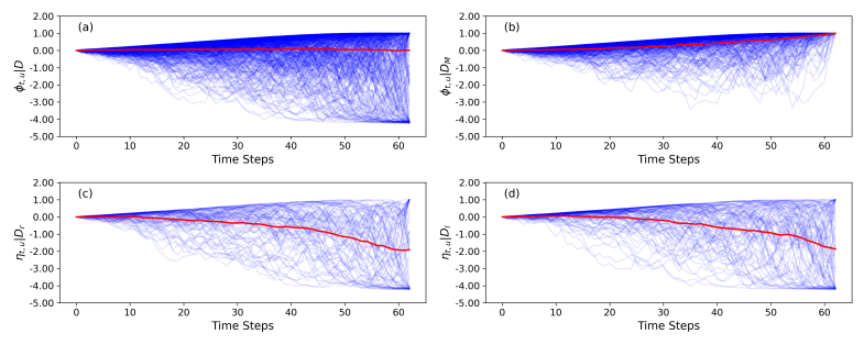
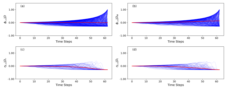
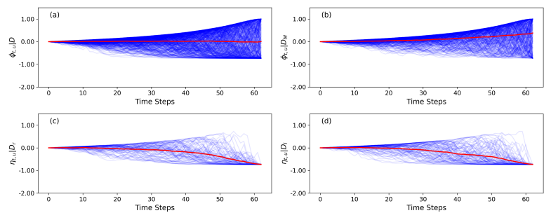
In this section, Moneyness is the sole variable determining the control process . Figures 2, 3, and 4 depict the distributions of potential profits and risks for values of 0.12, 0.06, and 0.00, respectively. The red line in each figure is the expectation process, denoted by or .
The options in Figure 2 are deep Out-Of-The-Money (OTM), resulting in the distribution spanning a wide range of values from [-4,1] and for all (Figure 2 (a)). In a sideways market (Figure 2(b)), exhibits a convex increase. However, the risk associated with this portfolio is significant, as illustrated in Figures 2(c) and 2(d), where shows a concave decrease as time approaches the option expiration date.
In contrast, the options in Figure 3 are slightly OTM, meaning their strike prices are closer to the underlying price compared to the previous case. In Figure 3(a), the distribution of becomes denser within the range of [-1.2,1]. In Figures 3(c) and 3(d), both and exhibit a concave decrease over time, but the maximum loss is significantly reduced compared to that shown in Figures 2(c) and 2(d).
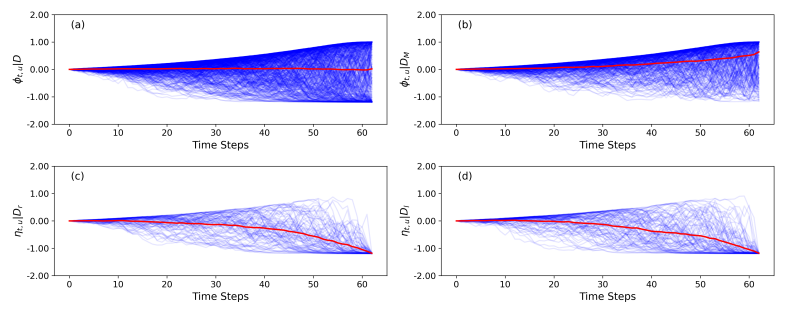
Figure 4 presents the at-the-money (ATM) case, where and , transforming the Iron Condor portfolio into an Iron Butterfly structure. The distribution of in Figure 4(a) is particularly appealing to investors, as it retains the maximum profit potential (albeit with a low probability) while capping the maximum loss at -0.2. However, Figure 4 shows that even under profitable market conditions, the is significantly lower compared to the previous cases where and .
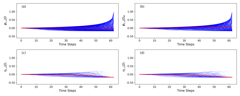
Figure 5 summarizes the influence of on portfolio performance. In Figure 5(a), increases exponentially with . The growing deviation between and as increases highlights the importance of employing an optimal stopping strategy for deep OTM portfolios.
In Figure 5(b), underperforms , suggesting that applying an optimal stopping strategy in sideways market conditions reduces profitability. This observation is consistent with the theoretical proof presented in Section 3.
In Figure 5(c), both and increase with . This is because increasing widens the span between and , thereby improving the success ratio. However, an interesting crossover is observed between and , indicating that for deep OTM options, holding the portfolio until expiration outperforms early stopping at the optimal time .
In Figure 5(d), and exhibit similar performance under the and datasets. Notably, consistently outperforms , indicating that applying an optimal stopping strategy generally reduces risks in volatile market conditions. For deep OTM options with , employing an optimal stopping strategy can significantly truncate risk within the range of -1.0.
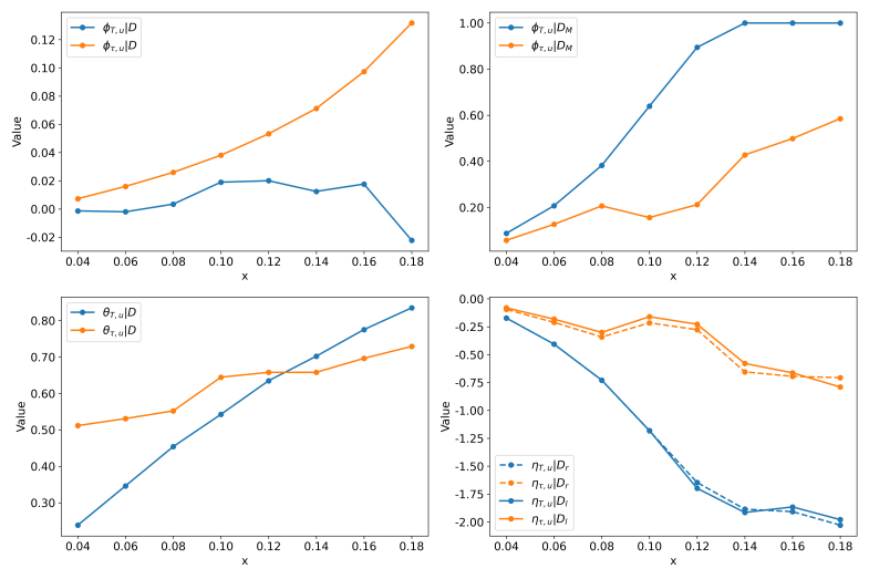
Table 1 provides comprehensive information about the performance of Iron Condor portfolios under various values of . The metrics , , , , and exhibit a positive relationship with , while all risk metrics, i.e., , , , and , show a negative relationship with .
Notably, the optimal stopping time ranges from 34 to 47 days out of the total 63-day period, corresponding to approximately 54% to 75% of the entire duration.
Interestingly, although employing the optimal stopping strategy reduces profitability in the sideways market (), it generally truncates risks and enhances overall profitability on , as evidenced by the metric.
| 0.18 | -0.02 | 0.13 | 43 | 0.83 | 0.73 | 1.00 | 0.59 | -2.03 | -0.71 | -1.98 | -0.79 |
| 0.16 | 0.02 | 0.10 | 43 | 0.78 | 0.70 | 1.00 | 0.50 | -1.91 | -0.70 | -1.87 | -0.66 |
| 0.14 | 0.01 | 0.07 | 44 | 0.70 | 0.66 | 1.00 | 0.43 | -1.89 | -0.66 | -1.92 | -0.58 |
| 0.12 | 0.02 | 0.05 | 34 | 0.63 | 0.66 | 0.89 | 0.21 | -1.65 | -0.28 | -1.70 | -0.23 |
| 0.10 | 0.02 | 0.04 | 34 | 0.54 | 0.64 | 0.64 | 0.16 | -1.18 | -0.22 | -1.18 | -0.16 |
| 0.08 | 0.00 | 0.03 | 47 | 0.45 | 0.55 | 0.38 | 0.21 | -0.73 | -0.34 | -0.73 | -0.30 |
| 0.06 | -0.00 | 0.02 | 47 | 0.35 | 0.53 | 0.21 | 0.13 | -0.41 | -0.21 | -0.41 | -0.18 |
| 0.00 | -0.00 | 0.01 | 47 | 0.24 | 0.51 | 0.09 | 0.06 | -0.17 | -0.10 | -0.17 | -0.08 |
4.2 Influence of Strikes Span
In this section, we focus on the strikes span , which governs the slope of the call and put spreads in an Iron Condor strategy.
Figure 6 presents a narrow-span case with . The risks ( and ) are well controlled, as shown in Figures 6(c) and (d). However, is approximately 0, indicating minimal profit potential.
In contrast, Figure 7 illustrates the distribution of in a wider-span case with . Here, exhibits a convex increase (Figure 7(b)), but the risks are significantly elevated compared to the case, as demonstrated in Figures 7(c) and (d).
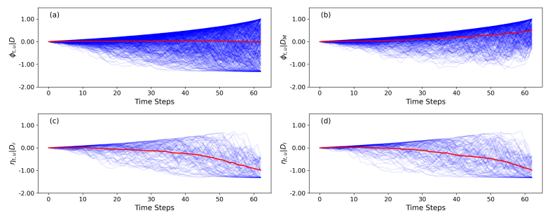
Figure 8 illustrates the impact of on portfolio performance. In Figure 8(a), exhibits a linear increase with , highlighting the significance of employing optimal stopping strategies for wide-span portfolios.
Under sideways market conditions, as shown in Figure 8(b), all optimal stopping strategies determined on underperform , consistent with the theoretical analysis presented in Section 3.
Figure 8(c) demonstrates that the success ratio consistently outperforms across all control values of , indicating that optimal stopping strategies enhance the likelihood of portfolio success.
Furthermore, Figure 8(d) presents the risk metrics in volatile markets. It is evident that for both and , the optimal stopping strategies effectively reduce risks.
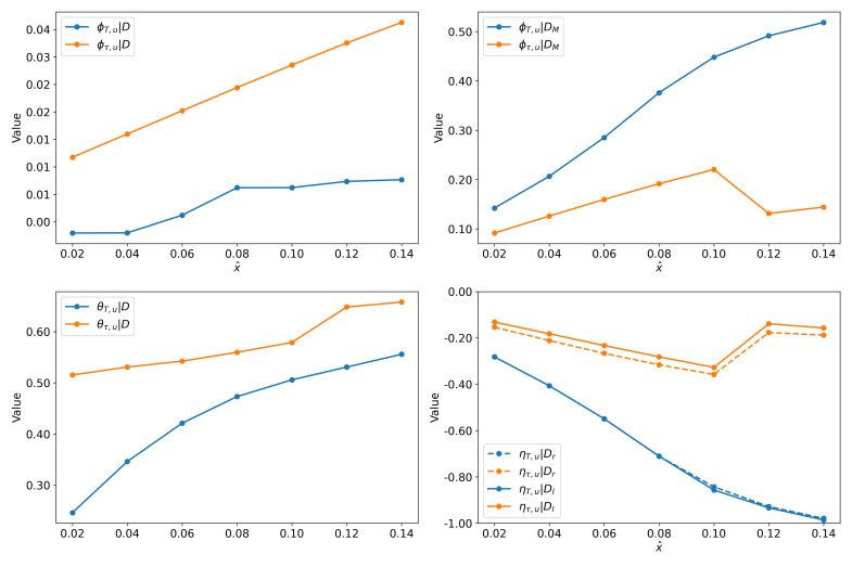
Table 2 summarizes the performance metrics of Iron Condor portfolios for various values of . Overall, it can be observed that , , , and increase as grows, indicating higher potential profits and success rates for wide-span cases. However, and also increase with , reflecting elevated risks for wider spans. The optimal stopping time varies from 34 to 47 days out of the total 63-day period, representing approximately 54% to 75% of the entire duration. Implementing optimal stopping strategies slightly improves potential profits while significantly reducing risk magnitudes.
| 0.02 | 0.00 | 0.00 | 47 | 0.51 | 0.24 | 0.14 | 0.09 | -0.28 | -0.15 | -0.28 | -0.19 |
| 0.04 | 0.00 | 0.01 | 47 | 0.53 | 0.34 | 0.20 | 0.12 | -0.40 | -0.21 | -0.40 | -0.18 |
| 0.06 | 0.00 | 0.02 | 47 | 0.54 | 0.42 | 0.28 | 0.15 | -0.54 | -0.27 | -0.54 | -0.23 |
| 0.08 | 0.01 | 0.02 | 47 | 0.55 | 0.47 | 0.37 | 0.19 | -0.71 | -0.32 | -0.71 | -0.28 |
| 0.10 | 0.01 | 0.03 | 47 | 0.50 | 0.57 | 0.44 | 0.22 | -0.84 | -0.36 | -0.85 | -0.33 |
| 0.12 | 0.01 | 0.03 | 34 | 0.53 | 0.64 | 0.49 | 0.13 | -0.92 | -0.18 | -0.93 | -0.14 |
| 0.14 | 0.01 | 0.03 | 34 | 0.55 | 0.65 | 0.51 | 0.14 | -0.97 | -0.19 | -0.98 | -0.16 |
5 Simulation Research on Asymmetry Iron Condor
This section examines the dynamics of an intriguing Asymmetric Iron Condor portfolio, which exhibits non-martingale behavior based on our simulation results. We define the asymmetry of an Iron Condor portfolio as the unbalanced moneyness between the bull put spread and the bear call spread. When , indicating that the put spread is deeper OTM, the portfolio is referred to as left-biased. Conversely, when , indicating that the call spread is deeper OTM, the portfolio is called right-biased.
To clarify the analysis, we first present a balanced baseline in Figure 9 and then provide a comparative discussion of the left-biased and right-biased portfolios in Figures 10 and 11
As shown in Figure 10(a), exhibits a slightly concave shape, suggesting non-martingale properties that may indicate arbitrage opportunities. Furthermore, and become asymmetric: the risk of increases significantly compared to the symmetric case shown in Figure 9(c), while the values of also increase compared to Figure 9(d). Notably, achieves positive values within , indicating reduced risk during this time interval.
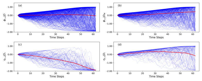
Figure 11 illustrates the right-biased case. Comparing Figure 11(a) with Figure 9(a), the Asymmetric Iron Condor introduces additional risk. Specifically, exhibits a convex increase. The risk metric , shown in Figure 11(c), displays a concave shape and achieves positive values before the 50th day, which is similar to the behavior of observed in Figure 10(d). However, in Figure 11(d), expands compared to that in Figure 9(d), indicating increased risk.
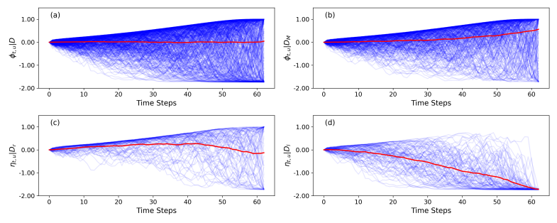
Figure 12 illustrates the impact of asymmetry on portfolio performance. In Figure 12(a), for left-biased portfolios, and overlap, indicating . Moreover, the large values of occurs in suggests that left-biased portfolios are more profitable. In contrast, for right-biased portfolios, underperforms the symmetric case, while surpasses both the symmetric case and the left-biased portfolios. This highlights the importance of employing an optimal stopping strategy in right-biased portfolios.
Under sideways market conditions, as shown in Figure 12(b), the left-biased portfolio significantly outperforms other scenarios. Furthermore, and achieve identical values, indicating that the optimal stopping time for the left-biased portfolio under sideways market conditions is .
Despite the data generator using tuned parameters from the real SPX market, some imperfect symmetric patterns can still be observed. In Figure 12(c), both and exhibit even symmetry around the symmetric portfolio. This indicates that asymmetric portfolios can achieve higher success rates compared to symmetric portfolios in the SPX market, although the latter case is more complex to analyze.
Moreover, in Figure 12(d), and display odd symmetry about the symmetric portfolio. For the left-biased portfolio, outperforms , while underperforms . This implies that when trading a left-biased portfolio, one should adopt an optimal stopping strategy in bearish markets but refrain from using such a strategy in bullish markets. Conversely, for the right-biased portfolio, the strategy should be reversed.
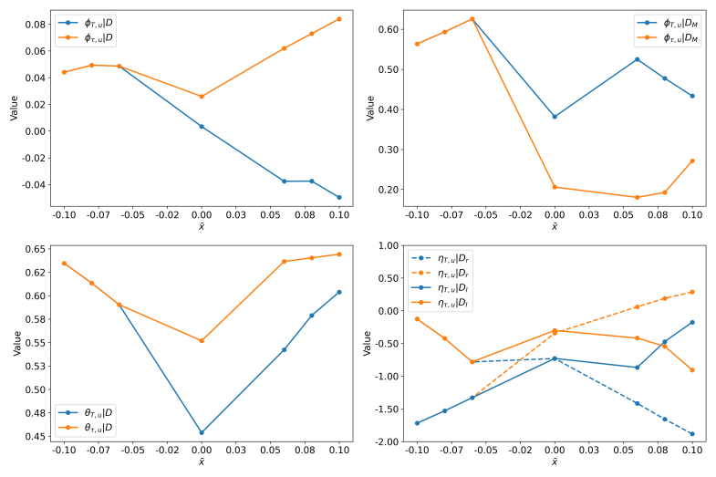
Table 3 summarizes the influence of on portfolio performance. Overall, the left-biased portfolio is observed to outperform the right-biased portfolio for the following reasons: 1. for all , whereas when . 2. of the left-biased portfolio strictly dominates that of the right-biased portfolio. 3. Under the same absolute level of , of the left-biased portfolio conditionally dominates that of the right-biased portfolio. 4. The maximum risk of the left-biased portfolio is lower than that of the right-biased ones.
However, the right-biased Iron Condor heavily depends on precise optimal stopping time to truncate extreme losses before expiration, which may cause to be dominated by . Nevertheless, it leads to strictly dominating , and strictly dominating .
The results are intriguing, and we aim to analyze them further. Since the S&P 500 index is predominantly bullish over time, establishing a left-biased portfolio provides greater tolerance for the upward movement of the underlying price while ensuring the terminal price remains within the profitable region. As a result, the left-biased Iron Condor is appealing for long-term holding and consistently outperforms the commonly used symmetric Iron Condor strategy.
From Table 3, the optimal stopping time for the right-biased portfolio varies between 34 and 41 days out of the total 63-day period, representing approximately 54% to 65% of the entire duration.
| 0.10 | -0.05 | 0.08 | 41 | 0.60 | 0.64 | 0.43 | 0.27 | -1.88 | 0.29 | -0.18 | -0.91 |
| 0.08 | -0.04 | 0.07 | 34 | 0.58 | 0.64 | 0.48 | 0.19 | -1.66 | 0.19 | -0.47 | -0.54 |
| 0.06 | -0.04 | 0.06 | 34 | 0.54 | 0.64 | 0.52 | 0.18 | -1.42 | 0.06 | -0.87 | -0.42 |
| 0.00 | 0.00 | 0.03 | 47 | 0.45 | 0.55 | 0.38 | 0.21 | -0.73 | -0.34 | -0.73 | -0.3 |
| -0.06 | 0.05 | 0.05 | 62 | 0.59 | 0.59 | 0.63 | 0.63 | -0.78 | -1.33 | -1.33 | -0.78 |
| -0.08 | 0.05 | 0.05 | 62 | 0.61 | 0.61 | 0.59 | 0.59 | -0.42 | -1.53 | -1.53 | -0.42 |
| -0.10 | 0.04 | 0.04 | 62 | 0.63 | 0.63 | 0.56 | 0.56 | -0.13 | -1.72 | -1.72 | -0.13 |
6 Validation on Actual SPX Market
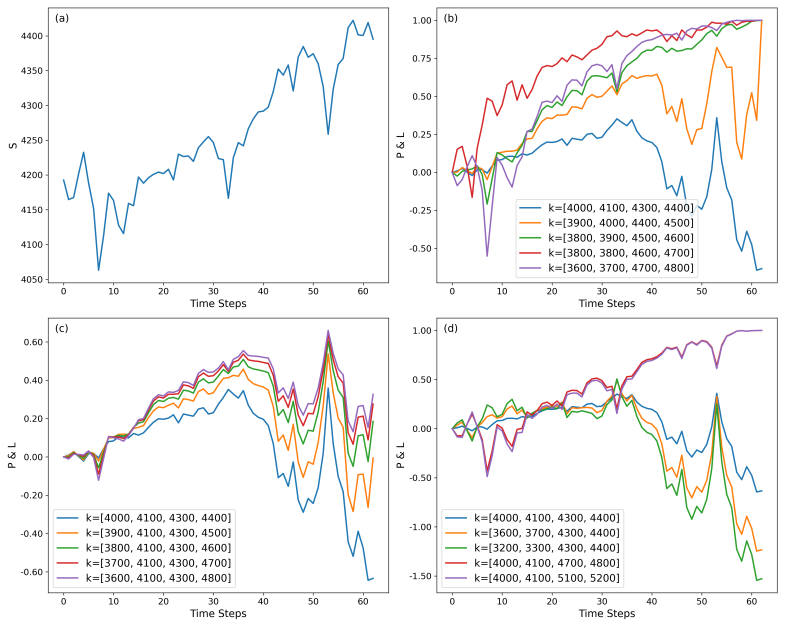
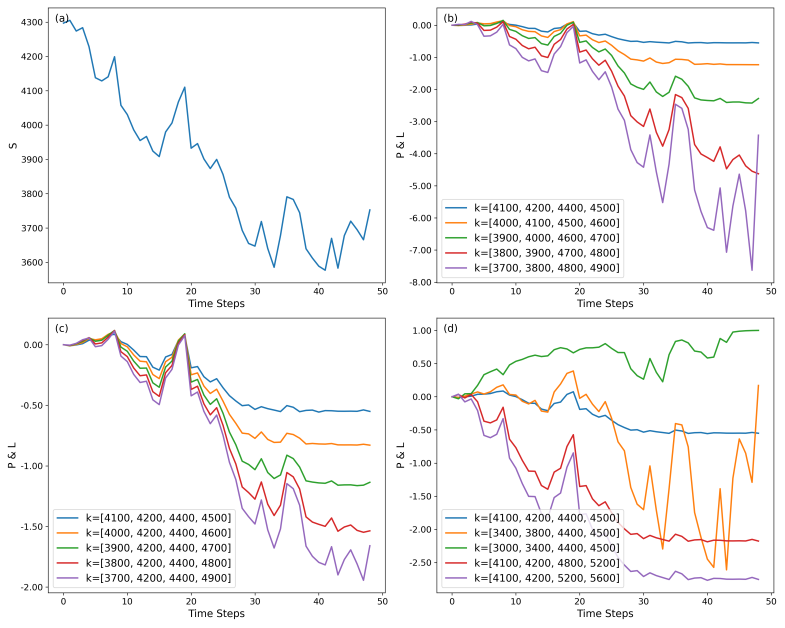
This section examines the performance of Iron Condor portfolios in the actual SPX market to validate the prior findings. We replace with (normalized) Profit & Loss (P&L) as the metric since only a single realization is available in real world. Specifically, we analyze three cases, with time frames spanning 63, 63, and 49 trading days prior to the options’ maturity dates of 2020-12-18, 2021-07-16, and 2022-10-21, respectively. The data used in this analysis is sourced from the OptionMetrics database.
Figure 13 presents the performance of portfolios with varying , , and during a bullish market (Figure 13(a)), where .
Figure 13(b) shows the P&L of portfolios with different values. Only the portfolio with the maximum (purple line) achieves its maximum profit, while 3 out of 5 portfolios result in negative returns, indicating a low success rate in this scenario.
Figure 13(c) shows the influence of . Unfortunately, none of these portfolios achieve positive return.
Promising results emerge in Figure 13(d), where a mirror symmetry of left-biased portfolios and right-biased portfolios about the symmetric portfolio is observed, which is very interesting. All left-biased portfolios achieve their maximum profit, whereas symmetric and right-biased portfolios all get negative return. This align with our simulation results that the left-biased Iron Condor can effectively handle risks resulting from bullish markets.
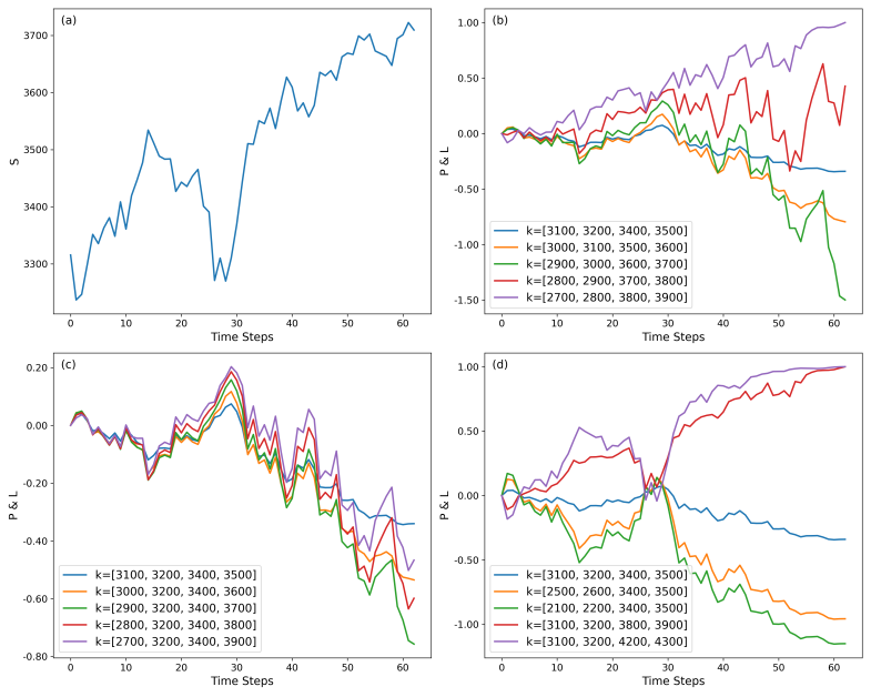
Figure 14 illustrates the P&L performance of portfolios under a sideways market condition (Figure 14(a)). In Figure 14(b), four out of five portfolios achieve their maximum profits, except the one with the smallest . This result aligns with our simulation findings that increasing improves the success rate. In Figure 14(c), for portfolios with a fixed , varying results in similar P&L patterns. Notably, three out of five portfolios yield positive returns. In Figure 14(d), all left-biased portfolios achieve their maximum profits, whereas the symmetric and right-biased portfolios exhibit poorer performance. This observation further supports the outcomes from our simulations. Moreover, adopting an optimal stopping strategy within the time interval [40, 50] days can significantly reduce overall risks, even if the profits of some portfolios are slightly diminished.
Finally, Figure 15(a) depicts an extreme bearish market. Under such conditions, changes in either or result in losses, as shown in Figures 15(b) and 15(c). However, constructing an asymmetric right-biased Iron Condor portfolio leads to positive returns, aligning with our findings from simulations.
7 Conclusion
This paper provides an in-depth analysis of the influence of the control process () on Iron Condor portfolios.
Initially, we assume the underlying price process is a bounded martingale within , and then prove a theorem that the optimal stopping time is if the Iron Condor strike structure satisfies for all .
We extend our study to more general scenarios by employing a simulation method based on the data generator derived from the Rough Heston model. We parameterize using four variables: moneyness (), strike span (), asymmetry degree () and optimal stopping time . The simulation results reveal the following key findings: (1) Asymmetric, left-biased Iron Condor portfolios with tend to be optimal in SPX markets, balancing profitability and risk management effectively; (2) Deep OTM Iron Condor portfolios improve profitability and success rates, but they also introduce the risk of extreme losses. Adopting an optimal stopping strategy can mitigate these losses, although it slightly reduces potential profits; (3) generally falls between 50% and 75% of the total duration, except for left-biased portfolios.
Finally, we validate our findings on the actual SPX market through three case studies covering bullish, sideways, and bearish market conditions, and the results support the simulation findings.
There are two limitations to the current research:
-
1.
The optimal stopping strategies derived from simulation methods need to be quantified and further analyzed.
-
2.
The approach requires a market trend forecasting method for effective strategy design.
The first limitation may be addressed using entropy-based methods, while the second could be further investigated through machine learning techniques in future research.
Declarations
-
1.
Funding:
This work is supported by National Natural Fundation of China (No.42402239) and Jiangsu University of Science and Technology Scientific Research Start-up Fund (No.1132932306). -
2.
Competing Interest declaration:
The author declare that they have no known competing financial interests or personal relationships that could have appeared to influence the work reported in this paper. -
3.
Data Availability Statement:
The author do not have permission to share data. -
4.
Author Contributions:
Qiguo Sun: Conceptualization, Investigation, Methodology, Analysis, Writing - Review& Editing.
Hanyue Huang: Conceptualization, Investigation, Methodology, Analysis, Writing - Review& Editing.
Xibei Yang: Methodology -
5.
Ethical statement:
All data handling procedures adhered to ethical guidelines for research.
References
- Abi Jaber (2019) Eduardo Abi Jaber. Lifting the heston model. Quantitative finance, 19(12):1995–2013, 2019.
- Bayer et al. (2016) Christian Bayer, Peter Friz, and Jim Gatheral. Pricing under rough volatility. Quantitative Finance, 16(6):887–904, 2016.
- Bennedsen et al. (2017) Mikkel Bennedsen, Asger Lunde, and Mikko S Pakkanen. Hybrid scheme for brownian semistationary processes. Finance and Stochastics, 21:931–965, 2017.
- Cohen (2005) Guy Cohen. The bible of options strategies: the definitive guide for practical trading strategies. Pearson Education, 2005.
- de Saint-Cyr (2023) Alberic de Saint-Cyr. A simple historical analysis of the performance of iron condors on the spx. Available at SSRN 4643378, 2023.
- Dupire et al. (1994) Bruno Dupire et al. Pricing with a smile. Risk, 7(1):18–20, 1994.
- Dziawgo (2020) Ewa Dziawgo. The iron condor strategy in financial risk management. Prace Naukowe Uniwersytetu Ekonomicznego we Wrocławiu, 64(2):33–44, 2020.
- El Euch et al. (2019) Omar El Euch, Jim Gatheral, and Mathieu Rosenbaum. Roughening heston. Risk, pages 84–89, 2019.
- Fadugba (2020) Sunday Emmanuel Fadugba. Homotopy analysis method and its applications in the valuation of european call options with time-fractional black-scholes equation. Chaos, Solitons & Fractals, 141:110351, 2020.
- Gatheral and Jacquier (2014) Jim Gatheral and Antoine Jacquier. Arbitrage-free svi volatility surfaces. Quantitative Finance, 14(1):59–71, 2014.
- Heston (1993) Steven L Heston. A closed-form solution for options with stochastic volatility with applications to bond and currency options. The review of financial studies, 6(2):327–343, 1993.
- Hu and Øksendal (2003) Yaozhong Hu and Bernt Øksendal. Fractional white noise calculus and applications to finance. Infinite dimensional analysis, quantum probability and related topics, 6(01):1–32, 2003.
- Ma and Wu (2022) Jingtang Ma and Haofei Wu. A fast algorithm for simulation of rough volatility models. Quantitative Finance, 22(3):447–462, 2022.
- Wang et al. (2022) Jian Wang, Shuai Wen, Mengdie Yang, and Wei Shao. Practical finite difference method for solving multi-dimensional black-scholes model in fractal market. Chaos, Solitons & Fractals, 157:111895, 2022.
- Wong and Bilokon (2024) Yat Chun Chester Wong and Paul Bilokon. Simulation of fractional brownian motion and related stochastic processes in practice: A straightforward approach. Available at SSRN, 2024.
- Woodard (2011) Jared Woodard. Iron Condor Spread Strategies: Timing, Structuring, and Managing Profitable Options Trades. Pearson Education, 2011.