Multiple truly topological unidirectional surface magnetoplasmons at terahertz frequencies
Abstract
Unidirectional propagation based on surface magnetoplasmons (SMPs) has recently been realized at the interface of magnetized semiconductors. However, usually SMPs lose their unidirectionality due to non-local effects, especially in the lower trivial bandgap of such structures. More recently, a truly unidirectional SMP (USMP) has been demonstrated in the upper topological non-trivial bandgap, but it supports only a single USMP, limiting its functionality. In this work, we present a fundamental physical model for multiple, robust, truly topological USMP modes at terahertz (THz) frequencies, realized in a semiconductor-dielectric-semiconductor (SDS) slab waveguide under opposing external magnetic fields. We analytically derive the dispersion properties of the SMPs and perform numerical analysis in both local and non-local models. Our results show that the SDS waveguide supports two truly (even and odd) USMP modes in the upper topological non-trivial bandgap. Exploiting these two modes, we demonstrate unidirectional SMP multimode interference (USMMI), being highly robust and immune to backscattering, overcoming the back-reflection issue in conventional bidirectional waveguides. To demonstrate the usefullness of this approach, we numerically realize a frequency- and magnetically-tunable arbitrary-ratio splitter based on this robust USMMI, enabling multimode conversion. We, further, identify a unique index-near-zero (INZ) odd USMP mode in the SDS waveguide, distinct from conventional semiconductor-dielectric-metal waveguides. Leveraging this INZ mode, we achieve phase modulation with a phase shift from - to . Our work expands the manipulation of topological waves and enriches the field of truly non-reciprocal topological physics for practical device applications.
I Introduction
Topological electromagnetics (EM) [1, 2, 3, 4] has gained significant attention due to its intriguing physics and potential applications [5]. One of the most remarkable features is the existence of unidirectional EM edge modes [6, 7] in non-trivial topological bandgaps, which can propagate in a single direction while suppressing backward refection, even in the presence of defects [8, 9]. These unidirectional edge modes arise from the breaking of time-reversal symmetry through an external magnetic field [10, 11], and were first proposed as analogues of quantum Hall edge states [12, 13] in photonic crystals (PhCs) [14]. Such PhCs-based unidirectional modes have been demonstrated both theoretically [15, 16] and experimentally [17, 18, 19, 20, 21, 22] at microwave frequencies.
As an alternative, surface magnetoplasmons (SMPs) have been proposed for unidirectional propagation due to their simple and robust structure [23, 24, 25, 26, 27, 28]. Recently, unidirectional SMPs (USMPs) have been realized using gyromagnetic (YIG) [29, 30, 31, 32] and gyroelectric (InSb) [33, 34, 35, 36] materials. In the terahertz (THz) regime, two types of USMP have been identified [37, 38, 39]. The first type, non-topological USMP, exists in the lower trivial bandgap of a magnetized semiconductor and transparent dielectric () waveguide [36, 40, 41], maintaining unidirectional characteristics due to non-reciprocal flat asymptotes [36]. However, these SMPs lose their strict unidirectionality when non-local effects are included [42], as the asymptotes vanish [43]. The second type, truly topological USMPs, exist in the upper non-trivial bandgap [39, 44, 45], at the interface between magnetized semiconductors and opaque dielectrics (), and are immune to non-local effect. These genuinely topological USMPs were first theoretically proposed and shown to exhibit robust unidirectionality against non-locality [39], and later experimentally demonstrated in a magnetized InSb-metal waveguide [46]. Further, a low-loss broadband USMP in the upper bandgap was proposed in an InSb-Si-air-metal waveguide [47], though only one truly USMP mode is supported in these waveguides.
Moreover, multimode interference (MMI) has been realized by coupling two or more conventional edge modes[48, 49], but these modes are bidirectional and suffer from back reflection. To overcome this limitation, PhCs-based MMI using multiple unidirectional modes has been proposed, effectively suppressing backscattering [50, 51]. More recently, unidirectional MMI based on PhCs has been experimentally demonstrated at microwave frequencies [52]. However, unidirectional MMI based on USMPs has not been reported at THz frequencies.
In this work, we propose a fundamental physical model for multiple truly USMP modes at THz frequencies, differing from previously proposed waveguides that support only one true USMP mode [39, 46, 47]. The model involves a semiconductor-dielectric-semiconductor (SDS) waveguide under opposing magnetic fields. We analytically derive and numerically analyze the dispersion in both local and non-local models, demonstrating that this waveguide supports two truly even and odd USMP modes in the upper bulk mode bandgap due to topological protection while these modes lose their unidirectionality in the lower bulk mode bandgap due to non-local effects. Using these two modes, we realize unidirectional SMP multimode interference (USMMI), which exhibits strong robustness against defects and eliminates backscattering, effectively overcoming the backscattering problem in conventional bidirectional waveguides; similarly to the PhCs-based MMI at microwave frequencies [52]. Additionally, we demonstrate a frequency- and magnetically-tunable arbitrary-ratio power splitter based on this robust USMMI, along with mode conversion capabilities. Notably, we report a unique index-near-zero (INZ) odd USMP mode in our waveguide, contrasting with conventional semiconductor-dielectric-metal waveguides that do not support the INZ mode [36]. This discovery enables efficient phase modulation with a phase shift of .
II Theoretical Physical model
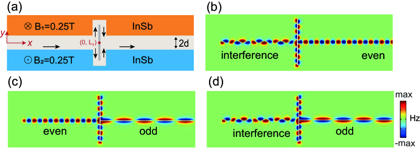
The basic physical model of multiple truly THz USMP modes in the SDS waveguide is illustrated in Fig. 1. In this part, we theoretically derive the dispersion equations for the SMP supported by the SDS structure in both local and non-local models.
II.1 Dispersion of SMP in the local model
First, we derive the dispersion equation of SMP in the local model. In our SDS system, the dielectric constant and thickness of the dielectric layer are and , respectively. To break the time-reversal symmetry of the system, opposing external magnetic fields ( and ) are imposed on the semiconductors in the direction. Consequently, the semiconductors exhibit gyroelectric anisotropy, with two corresponding relative permittivity tensors [36, 40]
| (1) |
with , (), and , where , is the electron scattering frequency, (where and are respectively the charge and effective mass of the electron) is the electron cyclotron frequency, is the plasma frequency, and is the high-frequency relative permittivity. In the magnetized semiconductor, the bulk modes have a dispersion relation of
| (2) |
for transverse-magnetic (TM) polarization, where is the propagation constant, is the vacuum wavenumber, and is Voigt permittivity. It has two bandgaps with . The upper boundaries of the lower and upper bandgaps are and by into Eq. (2). The lower boundary of the upper bandgaps are by into Eq. (2). The waveguide supports TM polarized SMP. Solving Maxwell’s equations with four continuous boundary conditions, the dispersion relation of SMP in the local model can be derived as (the details see Appendix A)
| (3) |
with
where , . By substituting into Eq. (3), the forward () and backward () asymptotic frequencies are obtained as and
Consider a special symmetric case of (corresponding to ), we have , , and , thus , then Eq. (3) becomes
| (4a) | |||
| (4b) | |||
for the even and odd modes, respectively.
II.2 Dispersion of SMP in the non-local model
We further derive the dispersion equation of SMP in the non-local model. When non-local effects are introduced into our system as a hydrodynamic model of free-electron gas [53, 54], the response of the semiconductors to EM field gives rise to an induced free electron current [39, 43, 42], which satisfies the hydrodynamic equation , where is the non-local parameter, and is a phenomenological damping rate. Maxwell’s equations can be expressed as and due to non-local effect. The dispersion relation of bulk modes can be found as [39, 47]
| (5) |
where , , and . By solving Eq. (5), we obtain two dispersion relations for the upper and lower bulk modes: and , where the lower cutoff frequencies are identical to and in the local model. Here, and are the propagation constants. In contrast to the local model, the upper cutoff frequency does not exist in the non-local model.
Combining hydrodynamic and Maxwell’s equations with six continuous boundary conditions, the SMP dispersion in the non-local model can be expressed as (the details see Appendix B)
| (6) |
with
where , , and
Consider a special symmetric case, we have , , and ; thus ; Eq. (6) becomes
| (7a) | |||
| (7b) | |||
for the even and odd modes, respectively.
III Simulation Results
In this part, we conduct a detailed numerical analysis of the SMP dispersion based on the derived equations in the SDS system and demonstrate many degrees of freedom to manipulate SMP modes, including interference, power, and phase, by full-wave simulation. Throughout the paper, the semiconductor is assumed to be InSb with , rad/s ( THz), and the dielectric layer is exemplified by silicon with a relative permittivity of .
III.1 The dispersion in the lower bulk mode bandgap
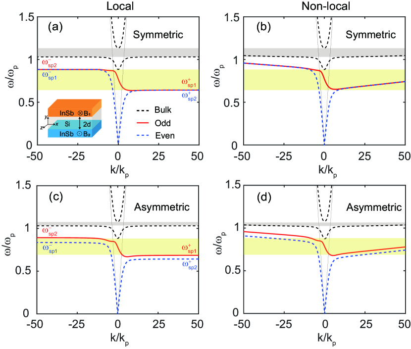
We first analyze the dispersion of SMP within the lower bulk mode bandgap. This bandgap ranges from to , where when . The special case of the symmetric () waveguide is considered. Using Eqs. (4) and (7), we numerically calculate the dispersion relations of SMPs in both local and non-local models, respectively. In the calculation, we ignore the effect of material loss (i.e., = 0) and take as an example. Figure 1(a) shows the dispersion of SMP in the symmetric waveguides for , corresponding to T. As expected, the SDS structure supports two SMP modes: odd mode (solid red line) and even mode (dashed blue line). These two modes exhibit identical asymptotic frequencies (, ). Moreover, these two modes propagate backward only within the frequency range [,], corresponding to [0.6425,0.8828]; As a result, a unidirectional propagation range is formed, as seen in the shaded yellow region in Fig. 1(a). However, when the non-local effects (non-local parameter m/s) are taken into account, the dispersion curves of the SMP modes differ significantly, as shown in Fig. 1(b). The forward and backward asymptotic frequencies of both modes vanish at large wave numbers, leading to the disappearance of the unidirectional propagation region within the lower bulk mode bandgap.
To further investigate the phenomenon of unidirectional disappearance induced by non-local effects, we analyze the dispersion in the common case of asymmetric waveguide () using Eqs. (3) and (6). As an example, and , which correspond to T and T, and the other parameters are identical to those of the symmetric waveguide. Figure 1(c) shows the dispersion curve for the local model. Due to the asymmetric structure, the SMP waveguide also supports even and odd modes. The asymptotic frequencies for the odd modes are and , while those for the even modes are and . As seen in the yellow shaded region, a unidirectional window based on horizontal asymptotes clearly occurs in [,], corresponds to [0.6859,0.8828]. For comparison, the dispersion curve for the non-local model is numerically calculated using Eq. (6). Similarly to the symmetric waveguide, Fig. 1(d) further demonstrates the disappearance of the asymptotic frequency when considering non-local effects, leading to the absence of the USMP window in the asymmetric waveguide. Therefore, the results demonstrate that for both symmetric and asymmetric waveguides, the SMP modes lose their unidirectionality in the lower bulk mode bandgap when non-local effects are considered.
III.2 The dispersion in the upper bulk mode bandgap
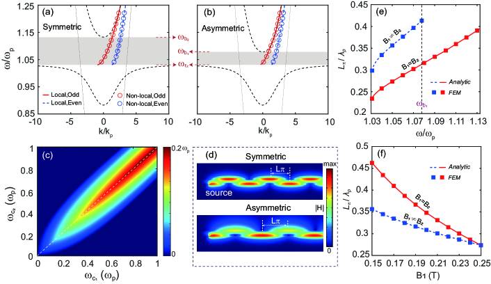
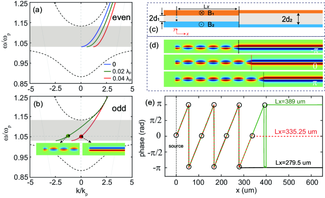
We further analyze the dispersion of SMP in the upper bulk mode bandgap [, ], where and , corresponding to the gray region in Fig. 1. We numerically calculate the dispersion of SMP in the local model, and the parameters are consistent with those in Fig. 1. Figure 2(a) shows the dispersion diagram for the symmetric waveguide with . As seen from the lines, this symmetric waveguide supports both odd (red solid line) and even (blue dashed line) USMP modes in upper bulk mode bandgap [, ], which corresponds to [,], marked by the grey shaded area. For comparison, the dispersion of SMP in the non-local model is also shown as circles in Fig. 2(a). Obviously, the dispersion curves for odd and even SMP modes almost completely coincide for both the local and non-local models. In contrast to the lower trivial bandgap, the SMP modes maintain their unidirectionality for small wavenumbers in the upper topologically non-trivial bandgap, even when non-local effects are considered. Figure 2(b) illustrates the dispersion curves for the asymmetric waveguide with and . Similarly to the symmetric results in Fig. 2(a), the USMP modes still exist, and the lines and circles almost completely overlap. However, the USMP band is compressed to the range [,], resulting from the asymmetric structure. When , the USMP bandwidth is characterized by
| (8) |
Note that when , the roles of and in the Eq. (8) will be interchanged. Figure 2(c) illustrates the variation of bandwidth with respect to and , which correspond to related parameters and . Due to and , the unidirectional bandwidth is magnetically-controllable by varying and . It is found that exhibits a local maximum when . The white dashed line indicates the distribution of this local maximum, which increases with .
These results confirm that in the upper bandgap, our waveguide supports two truly USMP modes at THz frequencies. The even and odd USMP modes maintain their unidirectionality when considering non-local effects, which is different from the situation in the lower bandgap. Moreover, the unidirectional characteristics of the SMP modes are equivalent in both the local and non-local models. Therefore, we will take the local model in the subsequent numerical calculations and simulations as an example, and our interest focuses on the upper bulk mode bandgap.
III.3 Unidirectional MMI based on two USMP modes
When two USMP modes are excited simultaneously and interact with each other in the silicon layer, unidirectional SMP multimode interference (USMMI) emerges. To verify this phenomenon, we simulate wave transmission in both symmetric and asymmetric waveguides with the finite element method (FEM) using COMSOL Multiphysics, as shown in Fig. 2(d). In the simulation, we position a magnetic current point source with a frequency of to excite the SMP and take into account the material loss (i.e., ). As expected, USMMI is realized at THz frequencies, and it can only propagate forward, not backward, in both symmetric and asymmetric waveguides. The -field distribution in the symmetric waveguide is identical at both InSb-Si interfaces, whereas it differs in the asymmetric waveguide due to structural asymmetry. Moreover, the -fields of USMMI are periodic with a period of 2, where the beat length is denoted by [55, 50]
| (9) |
where () is the propagation constant of the even (odd) mode, respectively.
To further investigate the characteristics of USMMI, we analyze the variation of with frequency and the external magnetic field. Figure 2(e) shows the analytical value of as a function of using Eq. (9) in the whole USMMI range. It is evident that increases with for both symmetric ( T) and asymmetric ( T and T) waveguides, corresponding to the red and blue lines, respectively. Figure 2(f) shows as a function of , where is fixed at as an example. As seen from the solid red line, the analytical monotonically decreases with varying from T to T, demonstrating the magnetically-controllable properties of USMMI by tuning two symmetric magnetic fields (). More interestingly, we achieve magnetically-controllable with a single-sided magnetic field, as indicated by the dashed blue line in Fig. 2(f). Here, is fixed at 0.25 T as an example. monotonically decreases with . Furthermore, we select multiple frequencies and magnetic fields to calculate the simulated with the full-wave FEM, as seen in the squares in Figs. 2(e) and 2(f), respectively. Obviously, the FEM results are in perfect agreement with the analytical values. Note that USMMI persists in the whole range, resulting from the magnetically-controllable USMMI band. This result confirms that USMMI is controllable by both frequency and the external magnetic field.
III.4 Frequency- and magnetically-tunable arbitrary-ratio power splitter based on USMMI
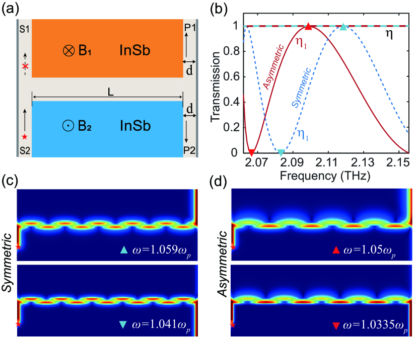
By controlling the beat length of MMI with external magnetic fields and frequencies, power manipulation has been achieved in topological PhCs at microwave frequencies [52]. Here, utilizing USMMI, we achieve arbitrary ratio power manipulation at THz frequencies. To verify this, we propose an H-shaped splitter, as shown in Fig. 3(a). The middle part is an SDS waveguide supporting USMMI, while the left and right parts are InSb-Si-Metal waveguides with silicon thickness [36], which has the same dispersion equation as given in Eq. (4a). A source, marked by a star, is placed at the input channel S2 to excite USMP and USMMI. Consequently, it is divided into the upper and lower outputs labeled as P1 and P2, respectively. To illustrate this, we perform full-wave simulations in both symmetric ( T) and asymmetric ( T, T) waveguides, and define the power ratio of channel P1 (P2) to channel S2 as (), and the total transmission as .
Figure 3(b) displays the transmission coefficients and versus for both splitters. oscillates arbitrarily between 0 and 1 in the unidirectional range from to . Owing to the backscattering-immune property of topologically USMP mode and the absence of reflection at the corners, remains close to 1 under low-loss conditions. For the symmetric waveguide, () at and () at ; whereas for the asymmetric waveguide, () at and () at . For clarity, the distributions of both waveguides are presented in Figs. 3(c) and 3(d), respectively. As expected, the power almost entirely flows into Channels P1 and P2 at and , and the interference length satisfies with an inverted (direct) image at the corner in the symmetric waveguide. Similarly, the power flow into Channel P1 (P2) at (), with in the asymmetric waveguide. The results demonstrate that a frequency-tunable arbitrary-ratio power splitter is realized using USMMI.
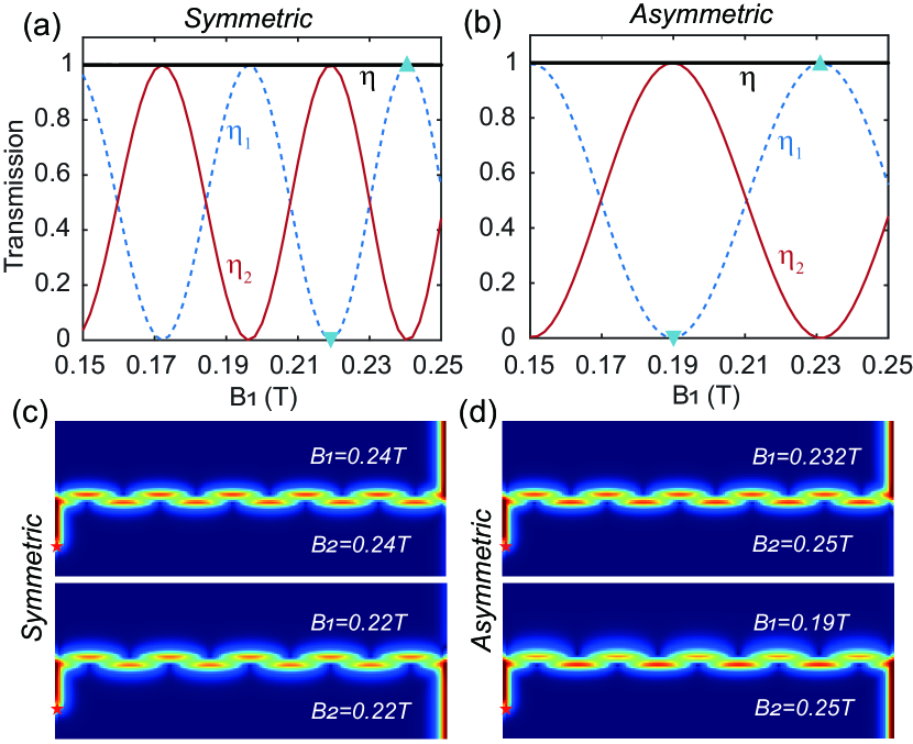

Furthermore, the magnetically-tunable power splitter based on USMMI is demonstrated. To verify this, the frequency is fixed at . Figure 4(a) shows the , , and versus by tuning two symmetric magnetic fields (). and vary continuously from to as changes within the range of [0.15 T, 0.25 T]. As a special case, and at T, and and at T. The corresponding full-wave simulation results are displayed in Fig. 4(c). As expected, the power respectively flows into channel P1 (P2) at T ( T), and the values of satisfy with an inverted (direct) image at the corner. This result confirms the arbitrary ratio power manipulation by the magnetic field. More importantly, we propose a single-sided magnetic control power splitter, which is much easier to operate than the both-sided control in practical applications. To demonstrate this, we set a fixed value of T as an example and resimulate by only adjusting . As seen in Fig. 4(b), the splitter achieves arbitrarily splitting ratios from 0 to 1 as expected. When T and T, the power is respectively directed to channels P1 and P2, as shown in Fig. 4(d), demonstrating magnetically-controllable power manipulation with only one magnetic field. Therefore, a USMMI-based power splitter has been demonstrated to achieve arbitrary ratios of power manipulation by the external magnetic field intensity and frequency, resulting from the frequency- and magnetically-controllable USMMI.
III.5 Robust USMMI at THz frequencies
To demonstrate the robustness of the USMMI, we introduce a square metallic defect of into the waveguide, as highlighted by the grey part in Fig. 5(a). We take a symmetric waveguide as an example. Figure 5(a) shows the simulated -field amplitudes for . It can be seen that the excited USMMI mode can smoothly bypass the defect and still travel forward without generating a backward wave from the defect. To clearly illustrate this phenomenon, the -field distributions along the upper InSb-Si interface are displayed for both cases with (dashed line) and without (solid line) defects in Fig. 5(c). As expected, the fields of USMMI remain unchanged before the defect and quickly recover the same amplitude after it. These results confirm the strong robustness of USMMI.
For comparison, we remove the external magnetic field from the waveguide in Fig. 5(a), effectively making it a conventional waveguide and resimulating it. Fig. 5(b) shows the simulated -field amplitudes with the defect. The excited wave is transmitted bidirectionally, and the H-field radiates everywhere in this waveguide. To clearly show this, the -field distributions for conventional waveguides with and without defects are plotted in Fig. 5(d). Without defects, the forward and backward fields are symmetric (solid line). When the defect is introduced, the field amplitudes become asymmetric (dashed line), with an increase before the defect and a decrease after it, demonstrating the backward reflection induced by the defect. These results demonstrate that our waveguide supports a robust USMMI mode without backscattering against defects, in contrast to the conventional bidirectional waveguide with backscattering.
III.6 Multiple modes conversion and phase modulation based on USMP
Based on the splitter, we further design a structure to achieve the conversion among multiple modes, as shown in Fig. 6(a). In this structure, the left and right parts are symmetric waveguides, and the silicon thickness is in the middle part. The input mode is equally divided and then recombines into a single output mode, with a phase difference , where is the initial phase difference, and is the position of the center of the metal bar along the -axis. It is found that the incident mode can be converted to an even mode when (where n is an integer) and to an odd mode when . The mode conversion satisfies the equations
| (10) |
where , this indicates that multimode conversion can be realized by tuning . We first consider a special case of mode conversion from an even mode to an odd mode, where . Here, we take =1.08 as an example, corresponding to . Thus, the theoretical value is found to be for using Eq. (10). To verify this, we perform full-wave simulations and the simulated -field for =1.08 is displayed in Fig. 6(c). The even mode is converted into odd modes when as expected. Furthermore, our FEM simulations demonstrate that the USMMI mode is converted into both even and odd modes when and , as shown in Figs. 6(b) and 6(d). It is found that , and the values of also satisfy Eq. (10) when . The results demonstrate that our structure achieves not only the conversion between USMMI and single mode but also the conversion between odd and even modes.
Interestingly, we further discover a unique index-near-zero (INZ) odd USMP mode without phase variation () supported by the SDS waveguide at THz frequencies, which is distinct from USMP in the conventional InSb-Si-Metal waveguides [36, 32]. These waveguides do not support INZ mode in the upper non-trivial bandgap. Based on the INZ odd mode in our waveguide, THz phase modulation is achieved. To illustrate this, we first calculate the dispersion curves of odd and even modes for different silicon thicknesses in the upper bandgap, as shown in Figs. 7(a) and 7(b), respectively. Both dispersion curves shift to the left as decreases. For a given frequency (), the propagation constant () of the even mode gradually approaches zero (), but as decreases, whose dispersion is the same as that of the conventional InSb-Si-Metal waveguides [36]. In contrast to the even mode, the most significant difference from the odd mode is the presence of the INZ mode (). As an example, the corresponding frequency for the INZ odd mode is when , marked by the red dot in Fig. 7(b). Unlike the regular even and odd modes, this INZ odd mode exhibits a stable phase. To clearly verify this, we perform full-wave simulations of the INZ mode at , as seen in the right inset of Fig. 7(b). For comparison, the result for the regular odd mode when is displayed in the left inset. It clearly demonstrates the zero-phase-shift transmission of the INZ odd mode, which is consistent with the theoretical results.
Next, utilizing the INZ odd USMP mode, we design a structure to achieve phase modulation with a phase shift of , as shown in Fig. 7(c). This structure consists of two symmetric waveguides with different , and the left part with supports a non-INZ odd mode, while the right part with supports an INZ odd mode. The point source (marked by the star) is positioned at a distance of from the interface (dashed line). By adjusting , we can precisely control the output phase ranging from - to . To verify this, we perform simulations for different values at . As an example, and , corresponding to the green and red dots. Figure 7(d) shows the simulated field amplitudes for um, um, and um, with the corresponding output phases being -, 0, and . To more clearly demonstrate this, we plot the phase of the field along the lower InSb-Si interface for these three values, as shown in Fig. 7(e). As expected, the output phases are -, 0, and due to the ’super-coupling’ effect [56]. These results show that our waveguide can realize all-optical phase modulation with a phase shift ranging from - to .
IV Conclusion
In this work, we have proposed and investigated a slab waveguide consisting of a dielectric layer sandwiched between two semiconductors subjected to opposite external magnetic fields. The dispersion characteristics of SMPs are analytically derived in both local and non-local models. Our numerical results show that the waveguide supports two truly USMP modes in the upper bulk mode bandgap, owning to topological protection. However, in the lower bulk mode bandgap, SMPs lose their strict unidirectionality due to non-local effects. By leveraging the two USMP modes, we demonstrate a magnetically-controllable USMMI at THz frequencies. Notably, USMMI exhibits strong robustness against defects, with no backscattering, in contrast to conventional bidirectional waveguides, which are susceptible to backscattering. Furthermore, we realized a frequency- and magnetically-tunable arbitrary-ratio splitter based on robust USMMI, enabling precise control of the splitter’s properties. Additionally, multimode conversion is achieved based on the splitter. We also identify a unique index-near-zero (INZ) odd USMP mode supported by our waveguide, distinct from conventional InSb-Si-Metal waveguides. Utilizing the INZ mode with zero phase shift transmission, we have designed a phase modulator that precisely controls the phase from - to . These results in mode manipulation utilizing USMP - encompassing interference, power, and phase control - offer a novel approach for the flexible manipulation of THz topological waves.
Acknowledgements.
This work was supported by National Natural Science Foundation of China (12464057, 12104203, 12264027, 61927813); Natural Science Foundation of Jiangxi Province (20242BAB25039, 20224BAB211015, 20242BAB20030, 20242BAB20024); Jiangxi Double-Thousand Plan (jxsq2023101069); Research Program of NUDT (ZK22-17). K. L. Tsakmakidis acknowledges funding within the framework of the National Recovery and Resilience Plan Greece 2.0, funded by the European Union NextGenerationEU (Implementation body: HFRI), under Grant No. 16909. K. L. Tsakmakidis was also supported by the General Secretariat for Research and Technology and the Hellenic Foundation for Research and Innovation under Grant No. 4509.Appendix A Derivation of dispersion formula in local model
In this appendix, we demonstrate Eq. (3) in the main text. In the local model, the magnetic field of SMP has non-zero components
| (11) | |||||
for the upper semiconductor layer, middle dielectric layer, and lower semiconductor layer, respectively. Using Maxwell’s equations and , the non-zero components ( and ) of the electric field in each layer can be directly derived from in Eq. (11), thus can be written as
| (12) | |||||
According to the boundary conditions of fields, and are continuous at boundaries and . Considering the continuity of , which requires and , we obtain from Eq. (11)
| (13) | ||||
Considering the continuity of , which satisfies and , we obtain from Eq. (12)
| (14) | ||||
By eliminating the four coefficients , , and in Eqs. (13) and (14), the dispersion relation of SMPs can be derived as
| (15) |
which corresponds to Eq. (3) of the main text.
Appendix B Derivation of formula in non-local model
In this appendix, we demonstrate Eq. (6) in the main text. When non-local effects are taken into account, the dispersion relation of SMP can be derived by solving the hydrodynamic and Maxwell’s equations as follows [39]
| (16) | ||||
Since the SDS waveguide only supports the TM mode (), the above equations for the lossless case () can be expressed as
| (17) | ||||
In the non-local model, the non-zero field components () and the normal component () are found to have the form [47]
| (18) |
for the upper semiconductor, and they can be written as
| (19) |
For the lower semiconductor, the parameters are given in the main text. According to the continuous boundary conditions of electric fields, we have and . Combining this with the first equations in Eq. (18) and Eq. (19) and the second equations in Eq. (12), it is found that
| (20) | ||||
According to the continuous boundary conditions of magnetic fields, and . By combining the third equation in Eqs. (18) and (19) with the second equation in Eq. (11), we obtain
| (21) | ||||
Unlike in the local model, an additional boundary condition is required: [43] at InSb-Si interface, which can be written as and . Using the last equations from Eq. (18) and Eq. (19), we have
| (22) | ||||
where and , with and , . By eliminating the six coefficients , , , , and in Eqs. (20)- Eq. (22), the dispersion relation of SMPs can be derived as
| (23) |
with
which corresponds to Eq. (6) of the main text.
References
- Lu et al. [2014] L. Lu, J. D. Joannopoulos, and M. Soljačić, Topological photonics, Nat. Photonics 8, 821 (2014).
- Hu et al. [2024] Y. Hu, M. Tong, T. Jiang, J.-H. Jiang, H. Chen, and Y. Yang, Observation of two-dimensional time-reversal broken non-Abelian topological states, Nat. Commun. 15, 10036 (2024).
- Prudêncio and Silveirinha [2022] F. R. Prudêncio and M. G. Silveirinha, Ill-Defined Topological Phases in Local Dispersive Photonic Crystals, Phys. Rev. Lett. 129, 133903 (2022).
- Rosiek et al. [2023] C. A. Rosiek, G. Arregui, A. Vladimirova, M. Albrechtsen, B. Vosoughi Lahijani, R. E. Christiansen, and S. Stobbe, Observation of strong backscattering in valley-Hall photonic topological interface modes, Nat. Photonics 17, 386 (2023).
- Bahari et al. [2017] B. Bahari, A. Ndao, F. Vallini, A. El Amili, Y. Fainman, and B. Kanté, Nonreciprocal lasing in topological cavities of arbitrary geometries, Science 358, 636 (2017).
- Gao et al. [2023] Z.-X. Gao, J.-Z. Liao, F.-L. Shi, K. Shen, F. Ma, M. Chen, X.-D. Chen, and J.-W. Dong, Observation of Unidirectional Bulk Modes and Robust Edge Modes in Triangular Photonic Crystals, Laser & Photonics Reviews 17, 2201026 (2023).
- Yu et al. [2023] X. Yu, J. Chen, Z.-Y. Li, and W. Liang, Topological large-area one-way transmission in pseudospin-field-dependent waveguides using magneto-optical photonic crystals, Photon. Res. 11, 1105 (2023).
- Ao et al. [2009] X. Ao, Z. Lin, and C. T. Chan, One-way edge mode in a magneto-optical honeycomb photonic crystal, Phys. Rev. B 80, 033105 (2009).
- Khanikaev and Alù [2024] A. B. Khanikaev and A. Alù, Topological photonics: robustness and beyond, Nat. Commun. 15, 931 (2024).
- Hadad and Steinberg [2010] Y. Hadad and B. Z. Steinberg, Magnetized Spiral Chains of Plasmonic Ellipsoids for One-Way Optical Waveguides, Phys. Rev. Lett. 105, 233904 (2010).
- Chen and Li [2022] J. Chen and Z.-Y. Li, Prediction and Observation of Robust One-Way Bulk States in a Gyromagnetic Photonic Crystal, Phys. Rev. Lett. 128, 257401 (2022).
- Haldane and Raghu [2008] F. D. M. Haldane and S. Raghu, Possible Realization of Directional Optical Waveguides in Photonic Crystals with Broken Time-Reversal Symmetry, Phys. Rev. Lett. 100, 013904 (2008).
- Prange and Girvin [1987] R. E. Prange and S. M. Girvin, The Quantum Hall Effect (Springer, New York, 1987).
- Joannopoulos et al. [2008] J. D. Joannopoulos, R. D. Meade, and J. N. Winn, Photonic Crystals: Molding the Flow of Light, 2nd ed. (Princeton University Press, Princeton, NJ, 2008).
- Wang et al. [2008] Z. Wang, Y. D. Chong, J. D. Joannopoulos, and M. Soljačić, Reflection-Free One-Way Edge Modes in a Gyromagnetic Photonic Crystal, Phys. Rev. Lett. 100, 013905 (2008).
- Lu et al. [2018] L. Lu, H. Gao, and Z. Wang, Topological one-way fiber of second Chern number, Nat. Commun. 9, 5384 (2018).
- Wang et al. [2009] Z. Wang, Y. D. Chong, J. D. Joannopoulos, and M. Soljačić, Observation of unidirectional backscattering-immune topological electromagnetic states, Nature 461, 772 (2009).
- Poo et al. [2011] Y. Poo, R.-x. Wu, Z. Lin, Y. Yang, and C. T. Chan, Experimental Realization of Self-Guiding Unidirectional Electromagnetic Edge States, Phys. Rev. Lett. 106, 093903 (2011).
- Wang et al. [2021] M. Wang, R.-Y. Zhang, L. Zhang, D. Wang, Q. Guo, Z.-Q. Zhang, and C. T. Chan, Topological One-Way Large-Area Waveguide States in Magnetic Photonic Crystals, Phys. Rev. Lett. 126, 067401 (2021).
- Zhou et al. [2020] P. Zhou, G.-G. Liu, Y. Yang, Y.-H. Hu, S. Ma, H. Xue, Q. Wang, L. Deng, and B. Zhang, Observation of Photonic Antichiral Edge States, Phys. Rev. Lett. 125, 263603 (2020).
- Chen et al. [2024] F. Chen, H. Xue, Y. Pan, M. Wang, Y. Hu, L. Zhang, Q. Chen, S. Han, G.-g. Liu, Z. Gao, P. Zhou, W. Yin, H. Chen, B. Zhang, and Y. Yang, Multiple Brillouin Zone Winding of Topological Chiral Edge States for Slow Light Applications, Phys. Rev. Lett. 132, 156602 (2024).
- Liu et al. [2025] G.-G. Liu, S. Mandal, X. Xi, Q. Wang, C. Devescovi, A. Morales-Pérez, Z. Wang, L. Yang, R. Banerjee, Y. Long, Y. Meng, P. Zhou, Z. Gao, Y. Chong, A. García-Etxarri, M. G. Vergniory, and B. Zhang, Photonic axion insulator, Science 387, 162 (2025).
- Yu et al. [2008] Z. Yu, G. Veronis, Z. Wang, and S. Fan, One-Way Electromagnetic Waveguide Formed at the Interface between a Plasmonic Metal under a Static Magnetic Field and a Photonic Crystal, Phys. Rev. Lett. 100, 023902 (2008).
- Hu et al. [2012] B. Hu, Q. J. Wang, and Y. Zhang, Broadly tunable one-way terahertz plasmonic waveguide based on nonreciprocal surface magneto plasmons, Opt. Lett. 37, 1895 (2012).
- Gao et al. [2016] W. Gao, B. Yang, M. Lawrence, F. Fang, B. Béri, and S. Zhang, Photonic Weyl degeneracies in magnetized plasma, Nat. Commun. 7, 12435 (2016).
- Tsakmakidis et al. [2021] K. L. Tsakmakidis, K. Baskourelos, and T. Stefański, Topological, nonreciprocal, and multiresonant slow light beyond the time-bandwidth limit, Appl. Phys. Lett. 119, 190501 (2021).
- Fernandes and Silveirinha [2019] D. E. Fernandes and M. G. Silveirinha, Topological Origin of Electromagnetic Energy Sinks, Phys. Rev. Appl. 12, 014021 (2019).
- Ozawa et al. [2019] T. Ozawa, H. M. Price, A. Amo, N. Goldman, M. Hafezi, L. Lu, M. C. Rechtsman, D. Schuster, J. Simon, O. Zilberberg, and I. Carusotto, Topological photonics, Rev. Mod. Phys. 91, 015006 (2019).
- Li et al. [2024] S. Li, K. L. Tsakmakidis, T. Jiang, Q. Shen, H. Zhang, J. Yan, S. Sun, and L. Shen, Unidirectional guided-wave-driven metasurfaces for arbitrary wavefront control, Nat. Commun. 15, 5992 (2024).
- Deng et al. [2015] X. Deng, L. Hong, X. Zheng, and L. Shen, One-way regular electromagnetic mode immune to backscattering, Appl. Opt. 54, 4608 (2015).
- Hong et al. [2019] L. Hong, Y. You, Q. Shen, Y. Wang, X. Liu, H. Zhang, C. Wu, L. Shen, X. Deng, and S. Xiao, Magnetic field assisted beam-scanning leaky-wave antenna utilizing one-way waveguide, Sci. Rep. 9, 16777 (2019).
- Zhou et al. [2022] Y. Zhou, P. He, S. Xiao, F. Kang, L. Hong, Y. Shen, Y. Luo, and J. Xu, Realization of tunable index-near-zero modes in nonreciprocal magneto-optical heterostructures, Opt. Express 30, 27259 (2022).
- Tsakmakidis et al. [2017a] K. L. Tsakmakidis, O. Hess, R. W. Boyd, and X. Zhang, Ultraslow waves on the nanoscale, Science 358, eaan5196 (2017a).
- Xu et al. [2023] J. Xu, Y. Luo, K. Yong, K. Baskourelos, and K. L. Tsakmakidis, Topological and high-performance nonreciprocal extraordinary optical transmission from a guided mode to free-space radiation, Commun. Phys. 6, 1 (2023).
- Shen et al. [2018] L. Shen, J. Xu, Y. You, K. Yuan, and X. Deng, One-Way Electromagnetic Mode Guided by the Mechanism of Total Internal Reflection, IEEE Photon. Technol. Lett. 30, 133 (2018).
- Tsakmakidis et al. [2017b] K. L. Tsakmakidis, L. Shen, S. A. Schulz, X. Zheng, J. Upham, X. Deng, H. Altug, A. F. Vakakis, and R. W. Boyd, Breaking Lorentz reciprocity to overcome the time-bandwidth limit in physics and engineering, Science 356, 1260 (2017b).
- Shen et al. [2015] L. Shen, Y. You, Z. Wang, and X. Deng, Backscattering-immune one-way surface magnetoplasmons at terahertz frequencies, Opt. Express 23, 950 (2015).
- Jin et al. [2016] D. Jin, L. Lu, Z. Wang, C. Fang, J. D. Joannopoulos, M. Soljačić, L. Fu, and N. X. Fang, Topological magnetoplasmon, Nat. Commun. 7, 13486 (2016).
- Gangaraj and Monticone [2019] S. A. H. Gangaraj and F. Monticone, Do truly unidirectional surface plasmon-polaritons exist?, Optica 6, 1158 (2019).
- Brion et al. [1972] J. J. Brion, R. F. Wallis, A. Hartstein, and E. Burstein, Theory of Surface Magnetoplasmons in Semiconductors, Phys. Rev. Lett. 28, 1455 (1972).
- Tsakmakidis et al. [2020] K. L. Tsakmakidis, Y. You, T. Stefański, and L. Shen, Nonreciprocal cavities and the time-bandwidth limit: comment, Optica 7, 1097 (2020).
- Raza et al. [2015] S. Raza, S. I. Bozhevolnyi, M. Wubs, and N. Asger Mortensen, Nonlocal optical response in metallic nanostructures, J. Phys.: Condens. Matter 27, 183204 (2015).
- Buddhiraju et al. [2020] S. Buddhiraju, Y. Shi, A. Song, C. Wojcik, M. Minkov, I. A. D. Williamson, A. Dutt, and S. Fan, Absence of unidirectionally propagating surface plasmon-polaritons at nonreciprocal metal-dielectric interfaces, Nat. Commun. 11, 674 (2020).
- Baskourelos et al. [2022] K. Baskourelos, O. Tsilipakos, T. Stefański, S. F. Galata, E. N. Economou, M. Kafesaki, and K. L. Tsakmakidis, Topological extraordinary optical transmission, Phys. Rev. Res. 4, L032011 (2022).
- Monticone [2020] F. Monticone, A truly one-way lane for surface plasmon polaritons, Nat. Photonics 14, 461 (2020).
- Liang et al. [2021] Y. Liang, S. Pakniyat, Y. Xiang, J. Chen, F. Shi, G. W. Hanson, and C. Cen, Tunable unidirectional surface plasmon polaritons at the interface between gyrotropic and isotropic conductors, Optica 8, 952 (2021).
- Yan et al. [2023] J. Yan, Q. Shen, H. Zhang, S. Li, H. Tang, and L. Shen, Broadband unidirectional surface plasmon polaritons with low loss, Opt. Express 31, 35313 (2023).
- Liu et al. [2022] L. Liu, Y. Wang, F. Zheng, and T. Sang, Multimode interference in topological photonic heterostructure, Opt. Lett. 47, 2634 (2022).
- Ma et al. [2024] X. Ma, Y. Li, Q. Xu, and J. Han, Terahertz plasmonic functional devices enabled by multimode interference, Opt. Laser Technol. 171, 110391 (2024).
- Liu and Wang [2023] L. Liu and Y. Wang, Unidirectional mode interference in magneto-optical photonic heterostructure, Opt. Laser Technol. 161, 109224 (2023).
- Skirlo et al. [2014] S. A. Skirlo, L. Lu, and M. Soljačić, Multimode One-Way Waveguides of Large Chern Numbers, Phys. Rev. Lett. 113, 113904 (2014).
- Tang et al. [2024] W. Tang, M. Wang, S. Ma, C. T. Chan, and S. Zhang, Magnetically controllable multimode interference in topological photonic crystals, Light Sci. Appl. 13, 112 (2024).
- Halevi [1995] P. Halevi, Hydrodynamic model for the degenerate free-electron gas: Generalization to arbitrary frequencies, Phys. Rev. B 51, 7497 (1995).
- Fonseca et al. [2024] G. R. Fonseca, F. R. Prudêncio, M. G. Silveirinha, and P. A. Huidobro, First-principles study of topological invariants of Weyl points in continuous media, Phys. Rev. Research 6, 013017 (2024).
- Soldano and Pennings [1995] L. Soldano and E. Pennings, Optical multi-mode interference devices based on self-imaging: Principles and applications, J. Lightwave Technol. 13, 615 (1995).
- Engheta [2013] N. Engheta, Pursuing Near-Zero Response, Science 340, 286 (2013).