We investigate the thermodynamics of asymptotically Anti-de Sitter charged and rotating black strings in extended phase space, in which the cosmological constant is interpreted as thermodynamic pressure and the thermodynamic volume is defined as its conjugate. We find, the thermodynamic volume, the internal energy, and the Smarr law. We study the thermal stability of solusions and show that some of the solutions have positive specific heat, which makes them thermodynamically stable. We also study the maximal efficiency of a Penrose process for solutions and find that an extremal rotating black string can have an efficiency of up to 50% compared to the corresponding value of 0%, when the cosmological constant is zero. We also find the equation of state for uncharged solutions. By comparing with the liquid-gas system, we observe that there is not a critical behavior to coincide with those of the Van der Waals system.

1 Introduction

Recently, there has been significant interest in the field of black hole thermodynamics in extended phase space, where the cosmological constant and/or other coupling parameters are treated as thermodynamic variables [1, 2, 3]. Although, the cosmological constant was traditionally considered a fixed parameter in the theory, however it could become a dynamical variable in gauged supergravity and string theories [4, 5].

The black hole thermodynamics in extended phase space has offered a variety of physical implications and applications. For example, investigating black hole phase transitions and the emergence of a research direction known as black hole chemistry [6, 7, 8]. In the contex of AdS/CFT, the holographic dual of the black hole thermodynamics in extended phase space on the CFT side has been widely explored. It also has been shown that the cosmological constant is not directly related to the CFT pressure but rather to the central charge [9, 10]. The thermodynamics in extended phase space can also find applications in the study of holographic complexity, and other research fields [11, 12, 13]. It is not only the cosmological constant that can be considered as a thermodynamic variable; but also other coupling parameters in higher curvature theories of gravity, just like those in Lovelock gravity, can also be regarded as thermodynamic variables [14, 15, 16, 17, 18]. An elegant derivation of extended thermodynamics from the extended Iyer-Wald formalism has also been fulfilled in [19].

Specific interest developed in the thermodynamics of charged black holes in asymptotically AdS spacetimes [20, 21], after the leading work by Hawking and Page [22], who observe that, there is a certain phase transition in the phase space of a Schwarzchild-AdS black hole. Since then, phase transitions and critical phenomena have been studied for more complicated backgrounds [23, 24]. The conventional phase space of a black hole consists only of entropy, temperature, charge and potential. Investigations of the critical behavior in the extended phase space seems more meaningful. With the extended phase space, the Smarr relation is satisfied in addition to the first law of thermodynamics, from which it is derived from scaling arguments. Furthermore, the resulting equation of state can be used for comparison with real world thermodynamic systems. This makes it evident that the phase space that should be considered is not the conventional one. Thermodynamic volume has been studied for a wide variety of black holes and is conjectured to satisfy the reverse isoperimetric inequality [4, 25]. The critical behavior of charged and rotating AdS black holes in $d$ spacetime dimensions, including effects from non-linear electrodynamics via the Born-Infeld action, in an extended phase space is also investigated in [26].

In this paper we are going to investigate the thermodynamic properties of the asymptotically AdS charged and rotating black strings in extended phase space. The asymptotically AdS charged rotating black strings first introduced in [27, 28]. The thermodynamic properties of solutions in conventional phase space are also investigated in [29].

The structure of our paper is arranged as follows. In the next section we review the metric and possible horizons of charged and rotating black strings. In Sec. 3, we review the thermodynamic properties, the first law of thermodynamics and Smarr law in ordinary phase space. In Sec. 4, we construct the theory of thermodynamics of charged and rotating black strings in extended phase space by considering the cosmological constant as thermodynamic pressure and introducing the extended first law of thermodynamics and Smarr law. We also find the thermodynamic volume, the mass and the internal energy as a function of thermodynamic variables. The thermal stability of solutions is also investigated in Sec. 5. In Sec. 6, we explore the maximal efficiency of a Penrose process. In Sec. 7, we extract the equation of state for uncharged black string and compare it with a liquid-gas system. Finally, Sec. 8 is devoted to conclusions.

2 Black strings

The metric of four-dimensional spacetime with cylindrical or toroidal horizons can be written as [27, 28]

$$ds^{2}=-f(r)\left(\Xi dt-ad\phi\right)^{2}+\frac{1}{f(r)}dr^{2}+\frac{r^{2}}{\ell^{4}}\left(adt-\Xi\ell^{2}d\phi\right)^{2}+\frac{r^{2}}{\ell^{2}}dz^{2},$$ (2.1)

where

$$\Xi=\sqrt{1+\frac{a^{2}}{\ell^{2}}}.$$ (2.2)

The mtric function $f(r)$ is given by

$$f(r)=\frac{r^{2}}{\ell^{2}}-\frac{m}{r}+\frac{q^{2}}{r^{2}},$$ (2.3)

and the gauge potential has the following form

$$A=-\frac{q}{r}\left(\Xi dt-ad\phi\right).$$ (2.4)

Here, the integration constants $m$ and $q$ are proportional to the mass and charge of black string and we call them the mass and charge parameters, respectively. The constants $a$ and $\ell$ have dimensions of length and can be interpreted as the rotation parameter and AdS radius, respectively. In the following, we are going to study the solutions with cylindrical symmetry. This implies that the spacetime admits a commutative two-dimensional Lie group $G_{2}$. The ranges of the time and radial coordinates are $-\infty<t<\infty,0\leq r<\infty$, and the topology of the horizon can be regarded as follows:

1. the flat torus $T^{2}$ with topology $S^{1}\times S^{1}$ (i.e., $G_{2}=U(1)\times U(1)$) and the ranges $0\leq\phi<2\pi,0\leq z<2\pi\ell$, which describes a closed black string,

2. the cylinder with topology $\mathbb{R}\times S^{1}$ (i.e., $G_{2}=\mathbb{R}\times U(1)$) and the ranges $0\leq\phi<2\pi,-\infty<z<\infty$, which describes a stationary black string,

3. the infinite plane with topology $\mathbb{R}^{2}$ and the ranges $-\infty<\phi<\infty,-\infty<z<\infty$, which does not rotate and can be interpreted as black hole.

We consider the topologies (i) and (ii) throughout the paper.

3 Thermodynamics

The relevant thermodynamic potentials are given by

$${\cal M}=\frac{1}{16\pi\ell}\left(3\Xi^{2}-1\right)m,\qquad T=\frac{3r_{+}^{4}-q^{2}\ell^{2}}{4\pi r_{+}^{3}\ell^{2}\Xi},\qquad{\cal S}=\frac{r_{+}^{2}\Xi}{4\ell},\qquad\Omega=\frac{a}{\Xi\ell^{2}},$$

$${\cal J}=\frac{3}{16\pi\ell}\Xi am,\qquad\qquad\qquad\Phi=\frac{q}{r_{+}\Xi},\qquad\quad{\cal Q}=\frac{q\Xi}{4\pi\ell},\qquad m=\frac{r_{+}^{3}}{\ell^{2}}+\frac{q^{2}}{r_{+}},$$ (3.1)

where $T$ is the Hawking temperature of the black string, $\Omega$ the angular velocity, $\Phi$ the electrostatic potential difference between infinity and the horizon. Here also, ${\cal M}$ is the mass, ${\cal S}$ the entropy, ${\cal J}$ the angular momentum and ${\cal Q}$ the electric charge, per unit volume of black string horizon. The thermodynamic potentials per unit length of black string horizon are given in [29]. They also can be derived from [30, 31] by setting the coupling constant to zero. In the above, we rewrite them per unit volume of black string horizon.

The event horizon is located at the largest root of the metric function (2.3) i.e., $f(r_{+})=0$. This equation leads to the mass parameter $m$, given in Eq. (3), in terms of the horizon radius $r_{+}$, the charge paramete $q$ and the AdS radius $\ell$.

If we consider the mass per unit volume of black string horizon ${\cal M}$ as a function of the entropy ${\cal S}$, the charge ${\cal Q}$, and the angular momentum ${\cal J}$ per unit volume of black string horizon i.e., ${\cal M}\left({\cal S},{\cal J},{\cal Q}\right)$, the first law of black hole thermodynamics,

$$d{\cal M}=Td{\cal S}+\Omega d{\cal J}+\Phi d{\cal Q},$$ (3.2)

is also astisfied for black string. The above first law is consistent with an integrated formula relating the black hole mass to other thermodynamic quantities known as Smarr relation:

$$0=T{\cal S}+\Omega{\cal J}.$$ (3.3)

In deriving this relation, we have used the fact that under a change of length scale, $\left({\cal M},{\cal S},{\cal J},{\cal Q}\right)\propto\left(L^{0},L^{1},L^{1},L^{0}\right)$. Applying the Euler’s theorem leads to the smarr relation.

4 Thermodynamic volume

When a cosmological constant, $\Lambda$, is included, there is a natural candidate for thermodynamic pressure,

$$P=-\frac{\Lambda}{8\pi}=\frac{3}{8\pi\ell^{2}},$$ (4.1)

and it is proposed that the thermodynamic volume of the black string per unit horizon volume, ${\cal V}$, be defined as the thermodynamic variable conjugate to $P$.

By allowing the pressure, the first law of black hole thermodynamics should then be modified to

$$d{\cal M}=Td{\cal S}+\Omega d{\cal J}+\Phi d{\cal Q}+{\cal V}dP.$$ (4.2)

The above extended first law is consistent with the following modified Smarr relation:

$$0=T{\cal S}+\Omega{\cal J}-2P{\cal V}.$$ (4.3)

In writting the above result we have used the fact that under a change of length scale $\left({\cal M},{\cal S},{\cal J},{\cal Q},P\right)\propto\left(L^{0},L^{1},L^{1},L^{0},L^{-2}\right)$ and apply Euler’s theorem.

The expression for mass ${\cal M}$ in terms of thermodynamic variables $({\cal S},P,{\cal J},{\cal Q})$ is

$$\!\!\!\!\!\!\!\!\!\!{\cal M}=\frac{1}{2^{3/4}\sqrt{3}\sqrt[4]{\pi}\sqrt[4]{P}\sqrt{\mathcal{S}}\left(32\pi^{3/2}\sqrt{2}\mathcal{J}^{2}P^{3/2}\mathcal{S}+\varUpsilon\right)^{3/2}}\left[32\pi^{3/2}\sqrt{2}\mathcal{J}^{2}P^{3/2}\mathcal{S}\varUpsilon+36864P^{4}\mathcal{S}^{8}\right.$$

$$\!\!\!\!\!\!\!\!\!\!\left.+55296\pi P^{3}\mathcal{Q}^{2}\mathcal{S}^{6}+32\pi^{3}P\mathcal{S}^{2}\left(64\mathcal{J}^{4}P^{2}+243\mathcal{Q}^{6}\right)+31104\pi^{2}P^{2}\mathcal{Q}^{4}\mathcal{S}^{4}+729\pi^{4}\mathcal{Q}^{8}\right],$$ (4.4)

where

$$\!\!\!\!\!\!\!\!\!\!\varUpsilon\equiv\left[110592P^{4}\mathcal{S}^{8}+165888\pi P^{3}\mathcal{Q}^{2}\mathcal{S}^{6}+32\pi^{3}P\mathcal{S}^{2}\left(64\mathcal{J}^{4}P^{2}+729\mathcal{Q}^{6}\right)\right.$$

$$\left.+93312\pi^{2}P^{2}\mathcal{Q}^{4}\mathcal{S}^{4}+2187\pi^{4}\mathcal{Q}^{8}\right]^{1/2}.$$ (4.5)

Differentiating with respect to $P$ according to Eq. (4.2) gives the thermodynamic volume per unit volume of black string horizon, in terms of thermodynamic variables as

$$\!\!\!\!\!\!\!\!\!\!\mathcal{V}=\left(\frac{\partial{\cal{\cal M}}}{\partial P}\right)_{\cal S,\cal J,\cal Q}=\frac{\sqrt{32\pi^{3/2}\sqrt{2}\mathcal{J}^{2}P^{3/2}\mathcal{S}+\varUpsilon}}{108\ 2^{3/4}\sqrt{3}\sqrt[4]{\pi}P^{5/4}\sqrt{\mathcal{S}}\left(8P\mathcal{S}^{2}+3\pi\mathcal{Q}^{2}\right)^{5}}\times$$

$$\left[256\pi^{5/2}\sqrt{2}\mathcal{J}^{2}P^{3/2}\mathcal{Q}^{2}\mathcal{S}\varUpsilon+884736P^{5}\mathcal{S}^{10}+1216512\pi P^{4}\mathcal{Q}^{2}\mathcal{S}^{8}+580608\pi^{2}P^{3}\mathcal{Q}^{4}\mathcal{S}^{6}\right.$$

$$\left.-8\pi^{4}P\mathcal{Q}^{2}\mathcal{S}^{2}\left(2048\mathcal{J}^{4}P^{2}+729\mathcal{Q}^{6}\right)+93312\pi^{3}P^{2}\mathcal{Q}^{6}\mathcal{S}^{4}-2187\pi^{5}\mathcal{Q}^{10}\right].$$ (4.6)

Transforming back to geometric variables $(r_{+},a({\rm or}~\Xi),q,\ell)$, one finds

$${\cal V}=\frac{\Xi^{2}r_{+}^{3}}{4\ell}+\frac{q^{2}\ell\left(3\Xi^{2}-4\right)}{12r_{+}}.$$ (4.7)

In terms of thermodynamic variables $({\cal S},P,\cal J,\cal Q)$ the temperature is,

$$\!\!\!\!\!\!\!\!\!\!T=\left(\frac{\partial{\cal M}}{\partial{\cal S}}\right)_{P,\cal J,\cal Q}=-\frac{9\sqrt{3}\left(\pi\mathcal{Q}^{2}-8P\mathcal{S}^{2}\right)\left(8P\mathcal{S}^{2}+3\pi\mathcal{Q}^{2}\right)^{3}\left(32\pi^{3/2}\sqrt{2}\mathcal{J}^{2}P^{3/2}\mathcal{S}\varUpsilon+\varUpsilon^{2}\right)}{2\ 2^{3/4}\sqrt[4]{\pi}\sqrt[4]{P}\mathcal{S}^{3/2}\varUpsilon\left(32\pi^{3/2}\sqrt{2}\mathcal{J}^{2}P^{3/2}\mathcal{S}+\varUpsilon\right)^{5/2}},$$

the angular velocity is

$$\Omega=\left(\frac{\partial{\cal M}}{\partial{\cal J}}\right)_{{\cal S},P,\cal Q}=\frac{16\ 2^{3/4}\pi^{5/4}\mathcal{J}P^{5/4}\sqrt{\mathcal{S}}}{\sqrt{3}\sqrt{32\pi^{3/2}\sqrt{2}\mathcal{J}^{2}P^{3/2}\mathcal{S}+\varUpsilon}},$$ (4.9)

and the electric potential is

$$\!\!\!\!\!\!\!\!\!\!\Phi=\left(\frac{\partial{\cal M}}{\partial\cal Q}\right)_{{\cal S},P,\cal J}=\frac{\sqrt[4]{2}\pi^{3/4}\mathcal{Q}\sqrt{32\pi^{3/2}\sqrt{2}\mathcal{J}^{2}P^{3/2}\mathcal{S}+\varUpsilon}}{27\sqrt{3}\sqrt[4]{P}\sqrt{\mathcal{S}}\left(8P\mathcal{S}^{2}+3\pi\mathcal{Q}^{2}\right)^{5}}\times$$

$$\!\!\!\!\!\!\!\!\!\!\left[-64\sqrt{2}\pi^{3/2}\mathcal{J}^{2}P^{3/2}\mathcal{S}\varUpsilon+110592P^{4}\mathcal{S}^{8}+165888\pi P^{3}\mathcal{Q}^{2}\mathcal{S}^{6}\right.$$

$$\left.+32\pi^{3}P\mathcal{S}^{2}\left(128\mathcal{J}^{4}P^{2}+729\mathcal{Q}^{6}\right)+93312\pi^{2}P^{2}\mathcal{Q}^{4}\mathcal{S}^{4}+2187\pi^{4}\mathcal{Q}^{8}\right].$$ (4.10)

Transforming back to geometric variables $(r_{+},a({\rm or}~\Xi),q,\ell)$, one finds the corresponding values in Eq. (3).

The internal energy per unit horizon volume of black string, ${\cal U}$ is the Legendre transformation of the mass (enthalpy),

$${\cal U}={\cal M}-P{\cal V},$$ (4.11)

where ${\cal M}$ is a function of $\cal S$, $P$, $\cal J$ and $\cal Q$ while $\cal U(\cal S,\cal V,\cal J,\cal Q)$ is a function of purely extensive variables. Then we get the usual form of the first law,

$$d{\cal U}=Td{\cal S}+\Omega d{\cal J}+\Phi d{\cal Q}-Pd{\cal V}.$$ (4.12)

Finding ${\cal U}$ in terms of purely extensive variables $(\cal S,\cal V,\cal J,\cal Q)$ is not possible. Because we can not solve Eq. (4) analytically to find $P$ in terms of $(\cal S,\cal V,\cal J,\cal Q)$.

In the next section, it will be more convenient to use the variables ${\cal S},P,\cal J$ and $\cal Q$, rather than $\cal S,\cal V,\cal J$ and $\cal Q$, in terms of which

$${\cal U}=\frac{1}{4\ 2^{3/4}\sqrt{3}\sqrt[4]{\pi}\sqrt[4]{P}\sqrt{\mathcal{S}}\left(32\pi^{3/2}\sqrt{2}\mathcal{J}^{2}P^{3/2}\mathcal{S}+\varUpsilon\right)^{3/2}}\times$$

$$\left[64\pi^{3/2}\sqrt{2}\mathcal{J}^{2}P^{3/2}\mathcal{S}\varUpsilon+36864P^{4}\mathcal{S}^{8}+110592\pi P^{3}\mathcal{Q}^{2}\mathcal{S}^{6}\right.$$

$$\left.+128\pi^{3}P\mathcal{S}^{2}\left(32\mathcal{J}^{4}P^{2}+243\mathcal{Q}^{6}\right)+93312\pi^{2}P^{2}\mathcal{Q}^{4}\mathcal{S}^{4}+3645\pi^{4}\mathcal{Q}^{8}\right].$$ (4.13)

In terms of geometrical variables,

$${\cal U}=\frac{r_{+}^{4}\left(3\Xi^{2}-2\right)+q^{2}\ell^{2}\left(3\Xi^{2}+2\right)}{32\pi r_{+}\ell^{3}}.$$ (4.14)

There is also a critical value of the black string charge parameter,

$$q_{\rm ext}=\frac{\sqrt{3}r_{+}^{2}}{\ell},$$ (4.15)

at which, the temperature vanishes, the horizon is degenerate and the black string is extremal. This leads to the following extermal value for mass parameter

$$m_{\rm ext}=\frac{4r_{+}^{3}}{\ell^{2}}.$$ (4.16)

Replacing the above two parameters into the thermodynamic potentials (3) and thermodynamic volume (4.7), one can easly find the extermal limit of thermodynamic variables.

5 Thermal stability

Here, we are going to investigate the thermal stability of the system in canonical ensemble. For an electrically neutral rotating black string, the specific heat at constant pressure per unit horizon volume is given by

$${\cal C}_{P} = T\left(\frac{\partial T}{\partial{\cal S}}\right)_{P,{\cal J}}^{-1}$$ (5.1)

$$= \frac{\mathcal{S}\left(\pi^{3}\mathcal{J}^{4}+54P\mathcal{S}^{6}-9\pi^{3/2}\mathcal{J}^{2}\sqrt{\pi^{3}\mathcal{J}^{4}+54P\mathcal{S}^{6}}\right)}{27P\mathcal{S}^{6}-40\pi^{3}\mathcal{J}^{4}}.$$

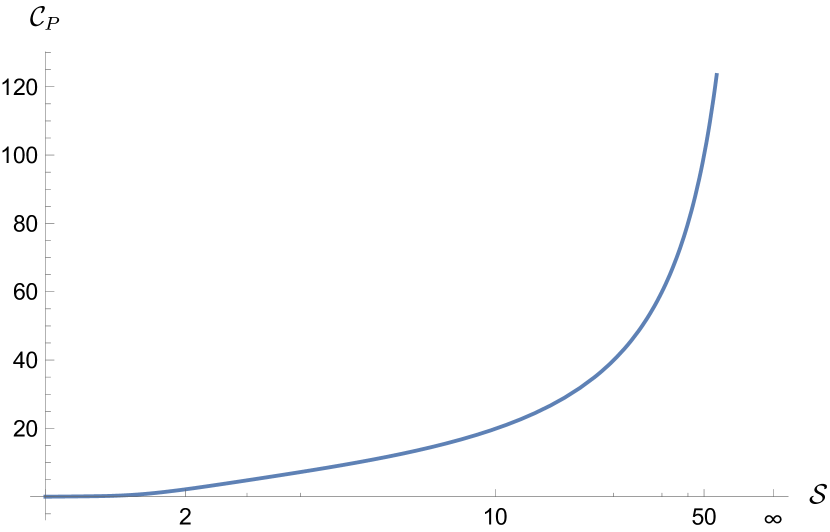
(a)

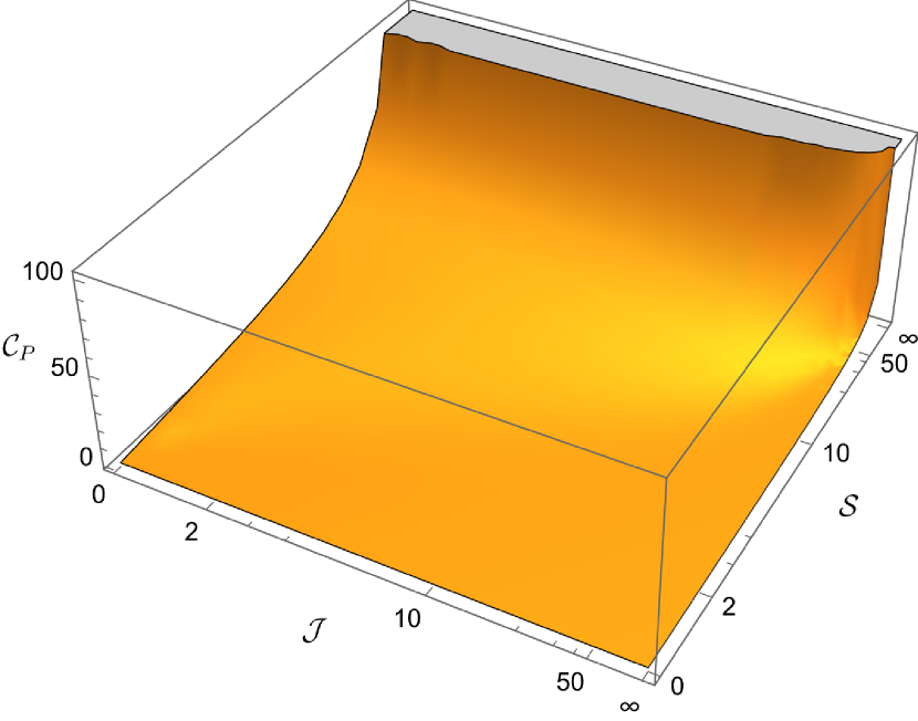
(b)

Figure 1: The profiles of the specific heat per unit horizon volume at constant pressure for uncharged rotating black string as a function of (a) ${\cal S}$ with fixed values $P=1$ and ${\cal J}=1$, (b) ${\cal S}$ and ${\cal J}$ at fixed value $P=1$.

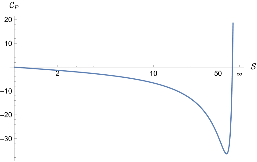
(a)

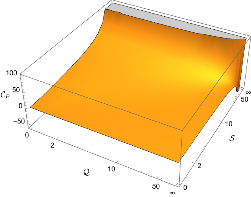
(b)

Figure 2: The profiles of the specific heat per unit horizon volume at constant pressure for charged rotating black string as a function of (a) ${\cal S}$ with fixed values $P=1$, ${\cal J}=1$ and ${\cal Q}=250$ (b) ${\cal S}$ and ${\cal Q}$ at fixed value $P=1$ and ${\cal J}=1$.

As illustrated in Fig. 1, the specific heat at constant pressure per unit horizon volume for uncharged rotating black string is positive and the solutions are thermodynamially stable.

In the case of charged solutions,

$${\cal C}_{P}\!\!\!\!\! = \!\!\!\!\!T\left(\frac{\partial T}{\partial{\cal S}}\right)_{P,{\cal J},{\cal Q}}^{-1}$$ (5.2)

$$= \!\!\!\!\!-2\mathcal{S}\left(\pi\mathcal{Q}^{2}-8P\mathcal{S}^{2}\right)\left(8P\mathcal{S}^{2}+3\pi\mathcal{Q}^{2}\right)\left[-288\sqrt{2}\pi^{7/2}\mathcal{J}^{2}P^{3/2}\mathcal{Q}^{4}\mathcal{S}\varUpsilon\right.$$

$$\!\!\!\!\!\left.+4608\pi^{5/2}\sqrt{2}\mathcal{J}^{2}P^{5/2}\mathcal{Q}^{2}\mathcal{S}^{3}\varUpsilon-18432\sqrt{2}\pi^{3/2}\mathcal{J}^{2}P^{7/2}\mathcal{S}^{5}\varUpsilon+7077888P^{6}\mathcal{S}^{12}\right.$$

$$\!\!\!\!\!\left.+15925248\pi P^{5}\mathcal{Q}^{2}\mathcal{S}^{10}+14929920\pi^{2}P^{4}\mathcal{Q}^{4}\mathcal{S}^{8}+144\pi^{5}P\mathcal{Q}^{4}\mathcal{S}^{2}\left(128\mathcal{J}^{4}P^{2}+2187\mathcal{Q}^{6}\right)\right.$$

$$\!\!\!\!\!\left.+192\pi^{4}P^{2}\mathcal{Q}^{2}\mathcal{S}^{4}\left(512\mathcal{J}^{4}P^{2}+10935\mathcal{Q}^{6}\right)+2048\pi^{3}P^{3}\mathcal{S}^{6}\left(64\mathcal{J}^{4}P^{2}+3645\mathcal{Q}^{6}\right)\right.$$

$$\!\!\!\!\!\left.+19683\pi^{6}\mathcal{Q}^{12}\right]\left[452984832P^{8}\mathcal{S}^{16}+1358954496\pi P^{7}\mathcal{Q}^{2}\mathcal{S}^{14}+1783627776\pi^{2}P^{6}\mathcal{Q}^{4}\mathcal{S}^{12}\right.$$

$$\!\!\!\!\!\left.+6912\pi^{6}P^{2}\mathcal{Q}^{6}\mathcal{S}^{4}\left(1024\mathcal{J}^{4}P^{2}+5103\mathcal{Q}^{6}\right)+262144\pi^{3}P^{5}\mathcal{S}^{10}\left(5103\mathcal{Q}^{6}-2560\mathcal{J}^{4}P^{2}\right)\right.$$

$$\!\!\!\!\!\left.+172032\pi^{4}P^{4}\mathcal{Q}^{2}\mathcal{S}^{8}\left(2048\mathcal{J}^{4}P^{2}+3645\mathcal{Q}^{6}\right)+110592\pi^{5}P^{3}\mathcal{Q}^{4}\mathcal{S}^{6}\left(1701\mathcal{Q}^{6}-512\mathcal{J}^{4}P^{2}\right)\right.$$

$$\!\!\!\!\!\left.+3779136\pi^{7}P\mathcal{Q}^{14}\mathcal{S}^{2}+177147\pi^{8}\mathcal{Q}^{16}\right]^{-1}.$$

As can be seen from Fig. 2, the solutions are thermodynamically unstable unless at large values of ${\cal Q}$.

6 The efficiency

In an isentropic, isobaric process, an uncharged black string can yield mechanical work by decreasing its angular momentum. If ${\cal J}$ is reduced from some finite value to zero, the efficiency is

$$\eta = \frac{{\cal U}({\cal J})-{\cal U}(0)}{{\cal M}}$$ (6.1)

$$= \frac{1}{12\left(\pi^{3}\mathcal{J}^{4}+54P\mathcal{S}^{6}+\pi^{3/2}\mathcal{J}^{2}\sqrt{\pi^{3}\mathcal{J}^{4}}+18P\mathcal{S}^{6}\right)}\times$$

$$\left[6\pi^{3}\mathcal{J}^{4}+54P\mathcal{S}^{6}+6\pi^{3/2}\mathcal{J}^{2}\sqrt{\pi^{3}\mathcal{J}^{4}}\right.$$

$$\left.-\sqrt[4]{2}3^{3/4}\sqrt[4]{P}\mathcal{S}^{3/2}\left(\pi^{3/2}\mathcal{J}^{2}+\sqrt{\pi^{3}\mathcal{J}^{4}+54P\mathcal{S}^{6}}\right)^{3/2}\right].$$

In terms of geometrical variables,

$$\eta=\frac{\Xi^{3/2}-3\Xi^{2}+2}{2-6\Xi^{2}}.$$ (6.2)

The asymptotically flat case is obtained by taking the limit $\ell\to\infty$, which requires $\Xi\to 1$. This leads to $\eta=0$. For finite $\ell$, the efficiency is greater than the asymptotically flat value. The greatest efficiency is for extremal black strings, when the Hawking tempereture vanishes. For a given $\mathcal{S}$, $P$ and $\mathcal{J}$, there is a maximal value of $\eta$ determined by demanding that $T=0$, which requires ${\cal S}=0$. Vanishing the entropy in Eq. (6.1) leads to $\eta=1/2$, as illustrated in Fig. 3.

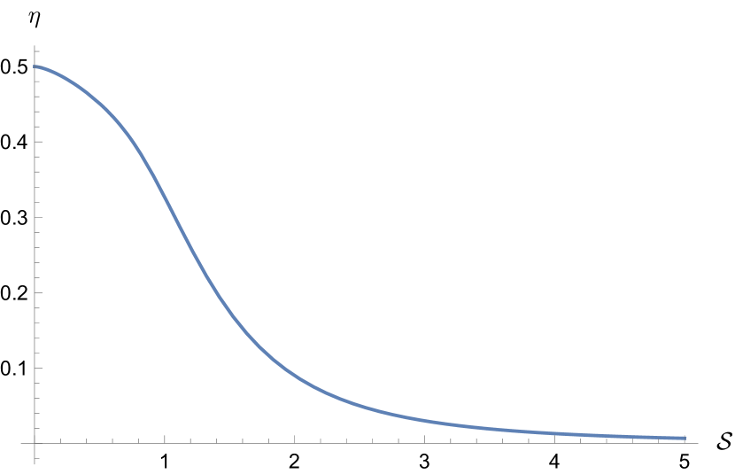
(a)

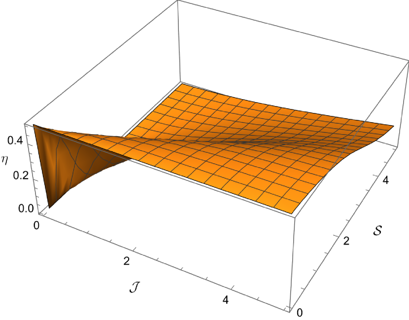
(b)

Figure 3: The profiles of efficiency as a function of (a) ${\cal S}$ with fixed values $P=1$ and ${\cal J}=1$, (b) ${\cal S}$ and ${\cal J}$ at fixed value $P=1$.

It also can be seen that the thermodynamic volume is a monotonically increasing function of ${\cal J}$, hence the volume decreases as ${\cal J}$ is lowered, keeping the area constant. The black string also heats up during the process, as illustrated in Fig. 4.

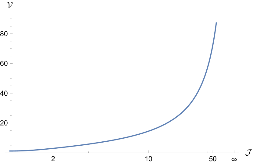
(a)

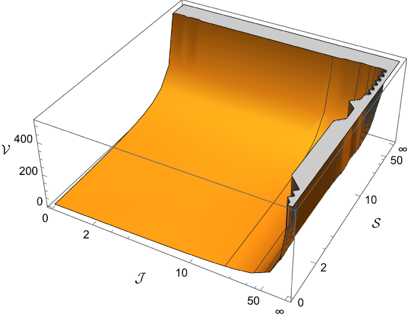
(b)

Figure 4: The profiles of the thermodynamic volume as a function of (a) ${\cal J}$ with fixed values $P=1$ and ${\cal S}=1$, (b) ${\cal J}$ and ${\cal S}$ at fixed value $P=1$.

When the black string is electrically charged and ${\cal J}$ and ${\cal Q}$ are both non-zero initially and are both decreased to zero, the efficiency is given by a complicated function of $\cal S$, $P$, $\cal J$ and $\cal Q$. But, in terms of geometrical variables, it takes the following simple form,

$$\eta=\frac{\left(-5\Xi^{3/2}+3\Xi^{2}+2\right)q^{2}\ell^{2}+\left(-\Xi^{3/2}+3\Xi^{2}-2\right)r_{+}^{4}}{2\left(3\Xi^{2}-1\right)\left(q^{2}\ell^{2}+r_{+}^{4}\right)}.$$ (6.3)

The efficiency for asymptotically flat case is obtained by taking the limit $\ell\to\infty$, which requires $\Xi\to 1$, and leads to $\eta=0$. The greatest efficiency is for extremal black strings, for which one can replace the mass parameter $q$ in the above equation from Eq. (4.15). Doing this gives

$$\eta=\frac{1-2\Xi^{3/2}}{3\Xi^{2}-1}+\frac{1}{2}.$$ (6.4)

As illustrated in Fig. 5, it can easily find that the maximum value of $\eta$ is $1/2$ which occurs for asymptotic value of $\Xi$.

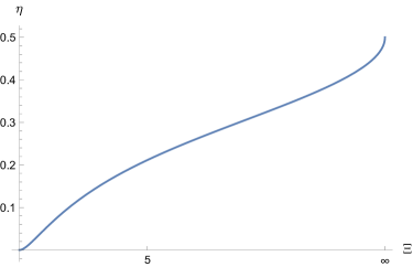
Figure 5: The profiles of efficiency as a function of $\Xi$.

7 Equation of state

When ${\cal Q}=0$, one can easily find the internal energy per unit horizon volume ${\cal U}$ as a function of purely extensive variables $({\cal S},{\cal V},{\cal J})$. To do so, we set ${\cal Q}=0$ in Eq. (4) for thermodynamic volume and solve it in terms of pressure, the result is

$$P=\frac{2\pi\mathcal{J}^{2}}{3\mathcal{V}^{2}}+\frac{6\mathcal{S}^{6}}{\pi\mathcal{V}^{4}}.$$ (7.1)

By setting ${\cal Q}=0$ in Eq. (4) for mass and plugging the above formula for pressure into it, one finds

$$\mathcal{M}=\frac{4\pi\mathcal{J}^{2}}{3\mathcal{V}}+\frac{8\mathcal{S}^{6}}{\pi\mathcal{V}^{3}}.$$ (7.2)

Replacing Eqs. (7.1) and (7.2) into Eq. (4.11), yields the following value for internal energy per unit horizon volume

$${\cal U}=\frac{2\pi\mathcal{J}^{2}}{3\mathcal{V}}+\frac{2\mathcal{S}^{6}}{\pi\mathcal{V}^{3}}.$$ (7.3)

with temperature

$$T=\left(\frac{\partial{\cal U}}{\partial\cal S}\right)_{{\cal V},\cal J}=\frac{12\mathcal{S}^{5}}{\pi\mathcal{V}^{3}}.$$ (7.4)

The equation of state, in the form of the relation between the pressure, the temperature and the thermodynamic volume per unit horizon volume, can be obtained by eliminating $\mathcal{S}$ between Eqs. (7.1) and (7.4),

$$P=\frac{2\pi\mathcal{J}^{2}}{3\mathcal{V}^{2}}+\frac{\sqrt[5]{\frac{\pi}{3}}T^{6/5}}{2\ 2^{2/5}\mathcal{V}^{2/5}}.$$ (7.5)

To make contact with the Van der Waals fluid in four dimensions, we should write the equation of state in terms of physical volume. To do so, we first set ${\cal Q}=0$ in Eq. (4) to find the thermodynamic volume for uncharged solutions. Then, we rewrite the result in terms of horizon radius by substituting the entropy from Eq. (3). The result reads

$$\mathcal{V}=\frac{\sqrt{\frac{\pi}{6}}\left(\sqrt{16\mathcal{J}^{2}+P^{2}r_{+}^{6}}+Pr_{+}^{3}\right)}{2\sqrt{P}}.$$ (7.6)

By plugging Eq. (7.6) into Eq. (7.5), one finds the pressure as

$$P = \frac{1}{2\sqrt{3}r_{+}^{5}}\left[r_{+}^{8}T^{2}+r_{+}^{20/3}T^{4/3}\sqrt[3]{12\mathcal{J}\left(18\mathcal{J}+\sqrt{324\mathcal{J}^{2}+3r_{+}^{4}T^{2}}\right)+r_{+}^{4}T^{2}}\right.$$ (7.7)

$$\qquad\qquad\left.+\frac{r_{+}^{28/3}T^{8/3}}{\sqrt[3]{12\mathcal{J}\left(18\mathcal{J}+\sqrt{324\mathcal{J}^{2}+3r_{+}^{4}T^{2}}\right)+r_{+}^{4}T^{2}}}\right]^{1/2}.$$

Making an expansion in powers of the angular momentum up to order ${\cal J}^{2}$, one finds,

$$P=\frac{T}{2r_{+}}+\frac{4\mathcal{J}^{2}}{r_{+}^{5}T}+{\cal O}\left({\cal J}^{4}\right).$$ (7.8)

Note that, in four dimensions

$$l_{p}^{2}=\frac{\hbar G}{c^{3}}.$$ (7.9)

To Translate the “geometric” equation of state (7.8) to a physical one, note that the physical pressure and temperature are given by

$${\rm Press}=\frac{\hbar c}{l_{p}^{2}}P,\qquad{\rm Temp}=\frac{\hbar c}{k}T.$$ (7.10)

When ${\cal J}=0$, multiplying (7.8) with $\hbar c/l_{p}^{2}$ we get

$${\rm Press} = \frac{k{\rm Temp}}{2r_{+}l_{p}^{2}}.$$ (7.11)

Comparing with the Van der Waals equation,

$$\left({\rm Press}+\frac{a}{v^{2}}\right)\left(v-b\right)=k{\rm Temp},$$ (7.12)

we conclude that, we should identify the specific volume $v$ with

$$v=2r_{+}l_{p}^{2}.$$ (7.13)

In geometric units, we have

$$r_{+}=kv,\quad k=\frac{1}{2}.$$ (7.14)

By setting ${\cal J}=0$ in Eq. (7.6), one finds

$$v=2\frac{\sqrt[6]{\frac{6}{\pi}}\sqrt[3]{\mathcal{V}}}{\sqrt[6]{P}}.$$ (7.15)

When ${\cal J}\neq 0$, by inserting (7.6) into (7.15), we get

$$\mathit{v}=\frac{2^{2/3}\sqrt[3]{\sqrt{16\mathcal{J}^{2}+P^{2}r_{+}^{6}}+Pr_{+}^{3}}}{\sqrt[3]{P}}.$$ (7.16)

Solving the above equation in terms of $r_{+}$ and substituting the result into Eq. (7.8), the equation of state can be rewritten as

$$P=\frac{P^{2/3}T\mathit{v}}{\sqrt[3]{P^{2}\mathit{v}^{6}-256\mathcal{J}^{2}}}+\frac{128\mathcal{J}^{2}P^{10/3}\mathit{v}^{5}}{T\left(P^{2}\mathit{v}^{6}-256\mathcal{J}^{2}\right)^{5/3}}+{\cal O}\left({\cal J}^{4}\right).$$ (7.17)

Making once again an expansion in powers of the angular momentum up to order ${\cal J}^{2}$, one finds,

$$P=\frac{T}{\mathit{v}}+\frac{640\mathcal{J}^{2}}{3T\mathit{v}^{5}}+{\cal O}\left({\cal J}^{4}\right).$$ (7.18)

The associated $P-v$ diagram for an uncharged rotating black string is displayed in Fig. 6.

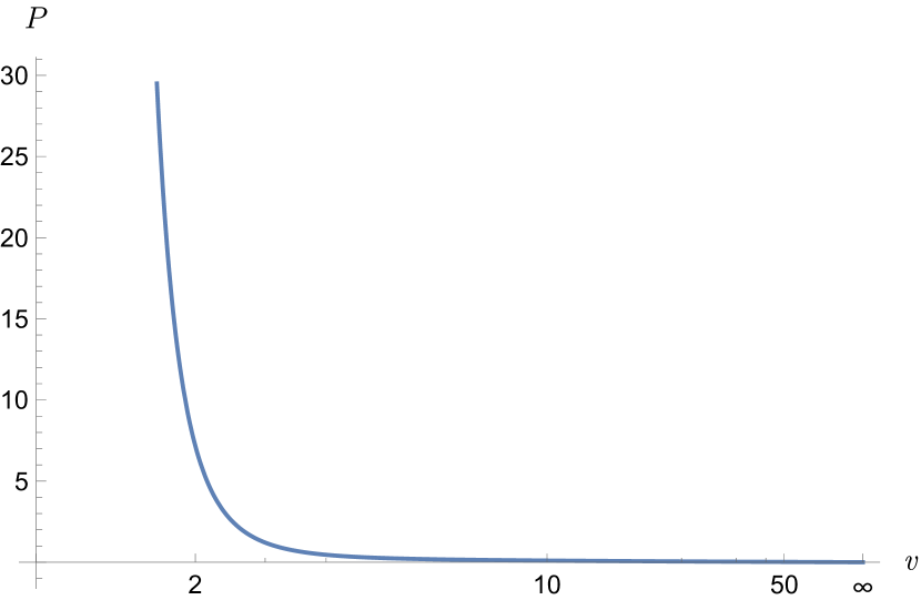
(a)

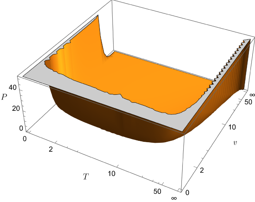
(b)

Figure 6: The profiles of $P$ as a function of (a) $v$ with fixed values $T=1$ and ${\cal J}=1$, (b) $v$ and $T$ at fixed value ${\cal J}=1$.

It can be seen there is no critical behvaior and as a result no Hawking-Page phase transition.

8 Conclusion

The thermodynamics of asymptotically AdS charged and rotating black strings in four-dimensional spacetime has been discussed in detail, with particular attention payed to the role of pressure and the volume. The cosmological constant is interpreted as a positive pressure and treated as a thermodynamic variable whose conjugate thermodynamic variable is a thermodynamic volume.

The thermal stability of solutions has been analyzed in canonical ensemble and it has been observed that the unchared solutions have positive specific heat at constant temperature and accordingly are thermodynamically stable while the charged ones are thermodynamically stable only for large values of charge.

In a Penrose process the volume decreases as the black string looses angular momentum and the $Pd{\cal V}$ term in the first law reduces the amount of energy available to do work. However a negative cosmological constant also extends the range of the angular momentum, pushing the maximum allowed value beyond that of the $\Lambda=0$ case, so that in fact more work can be extracted from an extremal black string in a spacetime that is asymptotically AdS than from one in a spacetime that is asymptotically flat. Efficiencies of up to 50% are theoretically achievable for a black string in asymptotically AdS spacetime, compared to 0% in asymptotically flat one.

The black string equation of state has been analysed in terms of pressure and physical volume. Non-zero angular momentum causes a rapid rise in pressure as the volume is reduced at constant temperature. We have found that, there is no critical behvaior and thus no Hawking-Page phase transition.

Let us close with some possible future explorations. It would be interesting to perform this kind of study, in higher dimensions. The asymptotically AdS charged and rotating solutions in $d$–dimensions have been presented in [32], and their thermodynamics in ordinary phase space has been explored in [33]. These solutions, depending on their global identifications, have toroidal, planar or cylindrical horizons and can be interpreted as black holes, or black strings/branes. Finding the solutions in the presence of nonlinear electrodynamics is also an interesting feature.

References

- [1] D. Kastor, S. Ray and J. Traschen, Class. Quant. Grav. 26, 195011 (2009) doi:10.1088/0264-9381/26/19/195011 [arXiv:0904.2765 [hep-th]].
- [2] B. P. Dolan, Class. Quant. Grav. 28, 125020 (2011) doi:10.1088/0264-9381/28/12/125020 [arXiv:1008.5023 [gr-qc]].
- [3] D. Kubiznak and R. B. Mann, JHEP 07, 033 (2012) doi:10.1007/JHEP07(2012)033 [arXiv:1205.0559 [hep-th]].
- [4] M. Cvetic, G. W. Gibbons, D. Kubiznak and C. N. Pope, Phys. Rev. D 84, 024037 (2011) doi:10.1103/PhysRevD.84.024037 [arXiv:1012.2888 [hep-th]].
- [5] P. Meessen, D. Mitsios and T. Ortin, JHEP 12, 155 (2022) doi:10.1007/JHEP12(2022)155 [arXiv:2203.13588 [hep-th]].
- [6] D. Kubiznak, R. B. Mann and M. Teo, Class. Quant. Grav. 34, no.6, 063001 (2017) doi:10.1088/1361-6382/aa5c69 [arXiv:1608.06147 [hep-th]].
- [7] S. W. Wei and Y. X. Liu, Phys. Rev. Lett. 115, no.11, 111302 (2015) [erratum: Phys. Rev. Lett. 116, no.16, 169903 (2016)] doi:10.1103/PhysRevLett.115.111302 [arXiv:1502.00386 [gr-qc]].
- [8] S. W. Wei, Y. X. Liu and R. B. Mann, Phys. Rev. Lett. 123, no.7, 071103 (2019) doi:10.1103/PhysRevLett.123.071103 [arXiv:1906.10840 [gr-qc]].
- [9] W. Cong, D. Kubiznak and R. B. Mann, Phys. Rev. Lett. 127, no.9, 091301 (2021) doi:10.1103/PhysRevLett.127.091301 [arXiv:2105.02223 [hep-th]].
- [10] M. B. Ahmed, W. Cong, D. Kubizňák, R. B. Mann and M. R. Visser, Phys. Rev. Lett. 130, no.18, 181401 (2023) doi:10.1103/PhysRevLett.130.181401 [arXiv:2302.08163 [hep-th]].
- [11] A. Al Balushi, R. A. Hennigar, H. K. Kunduri and R. B. Mann, Phys. Rev. Lett. 126, no.10, 101601 (2021) doi:10.1103/PhysRevLett.126.101601 [arXiv:2008.09138 [hep-th]].
- [12] B. Gwak, JHEP 11, 129 (2017) doi:10.1007/JHEP11(2017)129 [arXiv:1709.08665 [gr-qc]].
- [13] D. Harlow, B. Heidenreich, M. Reece and T. Rudelius, Rev. Mod. Phys. 95, no.3, 3 (2023) doi:10.1103/RevModPhys.95.035003 [arXiv:2201.08380 [hep-th]].
- [14] S. Dutta and G. S. Punia, Phys. Rev. D 106, no.2, 026003 (2022) doi:10.1103/PhysRevD.106.026003 [arXiv:2205.15593 [hep-th]].
- [15] D. Kastor, S. Ray and J. Traschen, Class. Quant. Grav. 27, 235014 (2010) doi:10.1088/0264-9381/27/23/235014 [arXiv:1005.5053 [hep-th]].
- [16] A. M. Frassino, D. Kubiznak, R. B. Mann and F. Simovic, JHEP 09, 080 (2014) doi:10.1007/JHEP09(2014)080 [arXiv:1406.7015 [hep-th]].
- [17] B. P. Dolan, A. Kostouki, D. Kubiznak and R. B. Mann, Class. Quant. Grav. 31, no.24, 242001 (2014) doi:10.1088/0264-9381/31/24/242001 [arXiv:1407.4783 [hep-th]].
- [18] M. Sinamuli and R. B. Mann, Phys. Rev. D 96, no.8, 086008 (2017) doi:10.1103/PhysRevD.96.086008 [arXiv:1706.04259 [hep-th]].
- [19] Y. Xiao, Y. Tian and Y. X. Liu, Phys. Rev. Lett. 132, no.2, 2 (2024) doi:10.1103/PhysRevLett.132.021401 [arXiv:2308.12630 [gr-qc]].
- [20] A. Chamblin, R. Emparan, C. V. Johnson and R. C. Myers, Phys. Rev. D 60, 064018 (1999) doi:10.1103/PhysRevD.60.064018 [arXiv:hep-th/9902170 [hep-th]].
- [21] A. Chamblin, R. Emparan, C. V. Johnson and R. C. Myers, Phys. Rev. D 60, 104026 (1999) doi:10.1103/PhysRevD.60.104026 [arXiv:hep-th/9904197 [hep-th]].
- [22] S. W. Hawking and D. N. Page, Commun. Math. Phys. 87, 577 (1983) doi:10.1007/BF01208266
- [23] M. Cvetic and S. S. Gubser, JHEP 04, 024 (1999) doi:10.1088/1126-6708/1999/04/024 [arXiv:hep-th/9902195 [hep-th]].
- [24] M. Cvetic and S. S. Gubser, JHEP 07, 010 (1999) doi:10.1088/1126-6708/1999/07/010 [arXiv:hep-th/9903132 [hep-th]].
- [25] M. Amo, A. M. Frassino and R. A. Hennigar, Phys. Rev. Lett. 131, no.24, 241401 (2023) doi:10.1103/PhysRevLett.131.241401 [arXiv:2307.03011 [gr-qc]].
- [26] S. Gunasekaran, R. B. Mann and D. Kubiznak, JHEP 11, 110 (2012) doi:10.1007/JHEP11(2012)110 [arXiv:1208.6251 [hep-th]].
- [27] J. P. S. Lemos, Phys. Lett. B 353, 46-51 (1995) doi:10.1016/0370-2693(95)00533-Q [arXiv:gr-qc/9404041 [gr-qc]].
- [28] J. P. S. Lemos and V. T. Zanchin, Phys. Rev. D 54, 3840-3853 (1996) doi:10.1103/PhysRevD.54.3840 [arXiv:hep-th/9511188 [hep-th]].
- [29] M. H. Dehghani, Phys. Rev. D 66, 044006 (2002) doi:10.1103/PhysRevD.66.044006 [arXiv:hep-th/0205129 [hep-th]].
- [30] H. R. Bakhtiarizadeh, Phys. Rev. D 105, no.6, 064037 (2022) doi:10.1103/PhysRevD.105.064037 [arXiv:2111.02663 [gr-qc]].
- [31] H. R. Bakhtiarizadeh, Nucl. Phys. B 987, 116083 (2023) doi:10.1016/j.nuclphysb.2023.116083 [arXiv:2112.11825 [gr-qc]].
- [32] A. M. Awad, Class. Quant. Grav. 20, 2827-2834 (2003) doi:10.1088/0264-9381/20/13/327 [arXiv:hep-th/0209238 [hep-th]].
- [33] M. H. Dehghani and A. Khoddam-Mohammadi, Phys. Rev. D 67, 084006 (2003) doi:10.1103/PhysRevD.67.084006 [arXiv:hep-th/0212126 [hep-th]].