A Novel Simulation Approach for Evaporation Processes in Small Gaps of Industrial Applications
Abstract
Long liquid retention times in industrial gaps, due to capillary effects, significantly affect product lifetime by facilitating corrosion on solid surfaces. Concentration-driven evaporation plays a major role in mitigating this corrosion. Accurate evaporation rate predictions are crucial for improved product design. However, simulating capillary-driven flows with evaporation in complex geometries is challenging, requiring consideration of surface tension, wetting, and phase-change effects. Traditional approaches, such as the Volume-of-Fluid method, are prone to curvature calculation errors and have long simulation times due to strict time step limitations.
This study introduces a novel semi-transient simulation approach for fast evaporation rate prediction in arbitrarily shaped cavities. The approach involves a unidirectional coupling circuit, simulating the fluid surface in Surface Evolver and combining it with a vapor-in-gas diffusion simulation in OpenFOAM. The approach assumes that the evaporation rate is calculated solely based on the conditions at a given liquid filling level, without considering the evaporation history. This allows for highly parallelized simulations, achieving simulation runtimes in the order of 10 minutes to cover up to 150 hours of physical time.
Numerical investigations are conducted for water evaporation in air at a temperature of 23°C and a relative humidity of 17%, for round and polygonal-shaped capillaries with inner diameters ranging from 1 mm to 13 mm. The results are validated using experimental data and show strong agreement. Simulations are also performed for complex industrial relevant gaps, demonstrating the applicability of the approach to a wide range of crevice geometries.
keywords:
Concentration-driven evaporation, Microfluidics, Wetting, Phase change, Numerical study, Surface Evolver, OpenFOAM[label1]organization=Robert Bosch GmbH, addressline=Robert-Bosch-Campus 1, city=Renningen, postcode=71272, country=Germany \affiliation[label2]organization=School of Mechanical and Safety Engineering, University Wuppertal, addressline=Gaußstraße 20, city=Wuppertal, postcode=42119, country=Germany
1 Introduction
Long liquid retention times in industrial gaps enable corrosion at solid surfaces which can be mitigated by evaporation of the liquid. Volatile liquids evaporate at a free liquid-gas surface and lead to a mass loss. The rate at which a liquid evaporates, depends on the geometry, thermal conditions and thermodynamical properties of the liquid and the surrounding gas. The numerical prediction of the evaporation rate in complex geometries is a part of recent research [1].
First investigations on the evaporation of water from capillaries go back to Stefan in 1871 [2]. He proposed an analytical model to calculate the evaporation rate from round capillaries based on Fick’s law of diffusion. Since then, experiments were conducted which confirm Stefan’s model [3, 4]. The evaporation rate in Stefan’s model depends on the mean diffusion length which describes the distance between the open capillary end and the mean meniscus position as depicted in Figure 1. Although this model is in good agreement with experimental results, it does not take the meniscus shape into account and assumes a flat surface.
In 1805 Young formulated a model to describe the change in pressure at a fluid-fluid interface, known as the capillary pressure, which depends on the interface curvature [5]. In the same year, this model was mathematically described by Laplace yielding the Young-Laplace equation [6]. Concus and Finn studied the shape of liquid surfaces in a wedge and showed that the Young-Laplace equation only has a bounded solution if , where is the contact angle as depicted in Figure 1 and is the half wedge angle [7].
Violating the condition by Concus and Finn leads to the formation of liquid fingers in the corners of the capillary as shown in Figure 1(b). Depending on corner geometry and liquid properties, the liquid fingers may reach up until the end of the capillary [8, 9] which results in a local reduction of diffusion length in the vicinity of the liquid fingers [4]. The reduced diffusion length in turn results in an enhanced evaporation, which could be confirmed in various experiments [10, 4].
Ransohoff and Radke performed numerical studies on non-circular capillaries to calculate corner liquid flow. They introduced a dimensionless flow resistance to account for corner angle, corner roundedness, surface shear viscosity and contact angle [8]. Chauvet et al. built up on their findings and showed that corner roundedness has a significant influence on the liquid finger geometry and might lead to depinning of the fingers from the top of the capillary [9]. Additionally, Chauvet et al. separated the drying process of capillaries into the three phases constant rate period (CRP), falling rate period (FRP) and receeding front period (RFP) depending on the free diffusion length [11]. CRP is characterized by the liquid-gas interface touching the open end of the capillary providing a nearly constant evaporation rate. Further evaporation leads to depinning of the liquid fingers and a drop in evaporation rate. In experiments, the depinning tends to coincide with the initiation of the FRP. Nevertheless, Keita et al. [10] showed for a rectangular channel where gravity was neglected, that liquid fingers might also be present in FRP. During RFP the meniscus shape can be assumed to stay constant, leading to an internal evaporation front receding inside the capillary [11].
Two centuries after Stefan’s findings, Camassel et al. proposed a simplified analytical model for square capillaries that neglects gravity and viscous effects to calculate the evaporation rate [3]. A few years later, Yiotis et al. developed an analytical model that also takes gravity and viscous effects into account [12] to determine the three-phase drying process in non-circular capillaries which was previously proposed by Chauvet et al. [11, 9]. Since analytical solutions are mostly limited to simple geometries, such as round capillaries, numerical models were developed to enable prediction of evaporation in arbitrary shaped geometries.
A major problem in common numerical methods that enable a full resolution of the free liquid surface, e.g. Volume-of-Fluid (VoF) or Front-Tracking, is the numerical handling of the mass source term at the liquid-gas interface due to evaporation in combination with the interface movement [13, 1, 14]. Irfan and Muradoglu developed a model to incorporate concentration-driven evaporation for the front-tracking method [15]. Their model is tested for 2D cases but they state that it could be easily adapted to 3D cases as well. Nonetheless, the Front-Tracking method is difficult to parallelize, thus it’s hardly applicable to complex simulations with several Million grid cells [16]. For the VoF approach a volume fraction field is used which allows interface capturing. The evaporation mass source term results in a non-divergence-free volume fraction field which tends to produce artificial spurious currents. To counteract this unintended behavior due to jump conditions at the interface, several methods were developed to dampen spurious currents [14, 17, 18, 13]. In all previously mentioned works the Navier-Stokes equations are solved in combination with an energy equation, which results in a high computational effort. However, Schweigler et al. used an Allen-Cahn phase-field approach where only an energy functional is solved to predict evaporation behavior in capillaries [4]. Although this method yields good results for arbitrary capillary shapes, it strongly relies on numerical parameters, gathered from calibration with experimental data.
Experimental investigations from Schweigler et al. [19] show that the evaporation of from a round capillary with 1 mm diameter can take more than 5 days. Thereby, significant time scale differences between evaporation and diffusion occur [20] that must be resolved by conventional methods with time steps in the order of . Considering small time steps and large time periods to be simulated, it is neither computationally nor temporally feasible to calculate the entire drying process of a capillary. Consequently, we present a decoupled approach where the fluid-fluid interface simulation is separated from the diffusion simulation. The goal of this work is to develop a generalized approach to calculate the evaporation rate from liquid to gas for various geometries, given specific thermodynamical boundary conditions. To the best of our knowledge there is no similar method in literature with a comparable speed while still providing accurate results.
2 Methodology
For the proposed quasi-steady approach, gas flow above and inside cavities is neglected to simplify the underlying Convection-Diffusion equation. Additionally, isothermal conditions are assumed such that the evaporation rate of liquid in a gas environment can be calculated for time steps individually according to
| (1) |
where is the gas density, is the diffusion coefficient of the evaporating species in the inert species, is the saturation vapor mass fraction, is the partial derivative of vapor mass fraction with respect to the interface normal vector and is the liquid-gas interface surface area which depends on the capillary geometry and the mean diffusion length . The times , at which the evaporation rate is evaluated, are unknown prior to the simulation. Thus, the function is solved which can be transformed into by substituting where is the evaporated vapor mass. Since , the time evaluates to
| (2) |
Utilizing Equation 2, the water mass at a certain point in time is implicitly determined as
| (3) |
In order to determine the function , the following three-step method is proposed:
-
1.
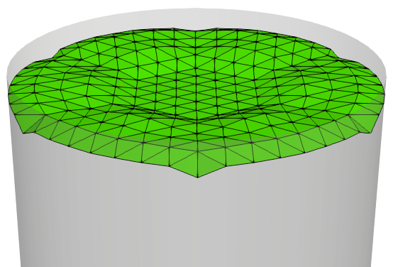
Surface formation simulation: The liquid surface shape is determined with Surface Evolver (SE). It is initialized as a plane and treated as a discrete differential geometry with movable vertices. The total surface energy is then minimized using a gradient-descent approach.
-
2.
Pre-processing: The capillary geometry is extended by an environment domain above the open end of the capillary. The liquid surface from SE divides the resulting domain into a liquid and a gas domain. By utilizing the OpenFOAM (OF) meshing utility snappyHexMesh (sHM), only the gas domain is meshed and the liquid domain is neglected.
-
3.
Diffusion simulation: The evaporation rate is determined using OF which solves the Laplace equation .
The previously described three-step process is depicted in Figure 2. The following sections describe the separate steps in more detail. The complete source code of the presented method is uploaded to the Bosch Research GitHub 111https://github.com/boschresearch/sepMultiphaseFoam/tree/publications/novelSimulationApproachForEvaporationProcesses.
2.1 Surface formation simulation
The surface shape is treated as a function of the crevice geometry and the mean diffusion length as given in Equation 1. For the surface formation simulation, the SE is used which was developed by Brakke in 1992 [21]. SE allows the user to create own geometries by defining vertices, edges and facets and then calculate the interface shape which is subject to different boundary conditions such as contact angle or surface tension. The algorithm behind SE is a gradient-descent method which minimizes the total surface energy of a given surface [21]. SE further provides features to manipulate the surface mesh such as refinement, equiangulation or vertex averaging which are described in the SE manual in more detail [22].
Since SE doesn’t provide a convergence algorithm, the solution depends on the sequence of iteration and surface manipulation steps. To prevent this, the convergence algorithm from the Surface Evolver - Fluid Interface Tool (SE-FIT®) is used which is developed at the Portland State University [23]. In order to serve the presented purpose, the algorithm settings are tuned which is further discussed in A.
Simulation setup
In this work, capillaries with various cross section shapes are considered. For all cases, a parameterized input file for SE is created with the mean diffusion length as a parameter. All geometries are centered around the origin and the bottom of the capillary is aligned with the plane at as visualized in Figure 1.
To simplify the file setup and reduce simulation runtime, completely wetted wall areas are omitted in the setup, thus leaving only the free fluid surface as depicted in Figure 3.
In the surface formation simulations, the liquid surface is initialized as a plane at where is the liquid filling height (see Figure 1) and then discretized as facets, edges and vertices. In order to comply with the contact angle boundary condition, the surface must be deformed. The surface deformation is done by calculating a vertex displacement vector depending on the local surface energy contribution, thus energy constraints must be implemented at the walls. The total liquid-gas surface energy at the walls is
| (4) |
with the wall area and the surface energy
| (5) |
between liquid and gas where is the surface tension coefficient. By applying Stoke’s theorem, the integral in Equation 4 can be transformed into a line integral around the three phase contact line of the surface. This calls for a divergenceless vector field , thus
| (6) |
where is a vector potential [22]. Substituting from Equation 6 in Equation 4 yields
| (7) |
In order to satisfy Equation 6, must be specified. In this work, the vector potential is set to
| (8) |
The initial filling height depends on the mean diffusion length as , thus the volume at the start of simulation is given as . Since the liquid is assumed to be incompressible, its volume must be conserved. In order to comply with volume conservation, the volume error at each iteration is calculated as
| (9) |
where is a facet of the surface and are the vertices z coordinates. The volume error then contributes to the surface energy loss function.
Further contributions to the surface energy calculation through gravity and surface tension in the bulk are taken care of by the SE and are described in the SE manual in detail [22].
2.2 Pre-processing
Since SE calculates a 2D surface in 3D space, the surface must be embedded into a volume mesh in order to simulate diffusion in the following three-dimensional vapor simulation step. Therefore, the capillary geometry is built in OF and extended by an environment over the open end of the capillary as depicted in Figure 4.
In order to create the curved meniscus shape as a lower boundary, the empty capillary is modeled first. As a second step the evolved interface from SE is scaled up by 1% in and direction to ensure that the interface completely intersects the outer capillary walls. The interface then splits the capillary into a liquid and a gas domain. As a third step, sHM is used to create a volume mesh for the upper gas domain.
2.3 Vapor diffusion simulation
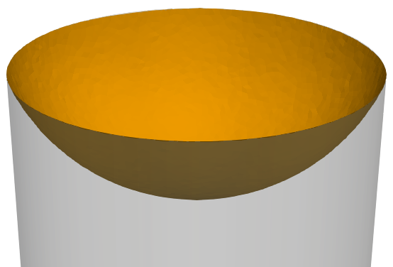
For the vapor diffusion simulation, the liquid phase is completely neglected leaving only the gas domain as depicted in Figure 5. The transport of multiple miscible species in a domain is governed by the convection-diffusion equation
| (10) |
for each species . In Equation 10, is the species density and is the velocity. In the following, a two-species system is assumed, consisting of an inert specie (index in) and a vapor specie (index v), i.e. no chemical reactions take place. Under this assumption the inert specie is omitted, since its mass fraction can be calculated as .
The inert gas at the interface is assumed to be constantly saturated. The vapor saturation mass fraction depends on the vapor saturation pressure which can be calculated using the Antoine equation
| (11) |
with the Antoine coefficients . The mole fraction of vapor in the gas mixture is given by
| (12) |
where is the vapor partial pressure. The mole fraction can then be converted to a mass fraction using
| (13) |
with the molar masses of vapor and inert specie respectively. The domain is assumed to be isothermal, hence evaporative cooling is not considered and no energy equation needs to be solved. In this case, the saturation vapor mass fraction is constant at the interface boundary.
To determine the quasi-steady solution of Equation 10, the temporal dependence . Air flow over the capillary is also neglected such that . Thus, the vapor in the domain is only subject to molecular diffusion. For liquid and gas at rest, the evaporation time scale is much smaller than the diffusion time scale . According to Sultan et al. [20], this further allows the assumption of a quasi-steady interface and that the distribution of vapor in air is a solution of the Laplace equation
| (14) |
Simulation setup
In the gas domain, only the vapor specie is considered and the inert specie is omitted as stated before. For all boundaries in Figure 5 and simulations, boundary conditions must be specified. They are listed in Table 1.
| boundary name | boundary type | value |
|---|---|---|
| interface | Dirichlet | |
| capillary walls | Neumann | |
| environment | Dirichlet |
To solve the Laplace Equation 14 for the given domain, a customized version of the laplacianFoam solver from OF is used, which is called steadyMolecularDiffusionFoam. The solver is adapted to calculate the steady-state Laplace solution by dropping all time-dependent terms in the laplacianFoam code. The numerical parameters that are used across all simulations are listed in Table 2.
| parameter/setting | value |
|---|---|
| solver | PCG |
| preconditioner | DIC |
| tolerance | |
| relTol | 0 |
| laplacianSchemes | Gauss linear corrected |
| 10 |
3 Results and discussion
Simulations are conducted for the evaporation of water in air for round and square capillaries according to the experiments from Schweigler [4]. A height of mm is used for all capillaries as in the experiments. The temperature °C and the pressure Pa are constant for all simulations. The environmental mass fraction is set according to a relative humidity of %. The temperature dependence of density and diffusion coefficient are incorporated using the ideal gas law for the humid air gas mixture and the Fuller method [24, 25] respectively. The thermodynamical properties of water and air under the given conditions are listed in Table 3.
| Property | Water | Air | Unit | Reference |
| Environment vapor mass fraction | - | Equations 11, 12 and 13 | ||
| Saturated vapor mass fraction | - | Equations 11, 12 and 13 | ||
| Density | [25] | |||
| Surface tension | [25] | |||
| Diffusion coefficient | [24, 25] | |||
| Contact angle (with borosilicate glass) | ∘ | [19] | ||
| Antoine coefficient | 23.4751 | - | [26] | |
| Antoine coefficient | 3978.205 | [26] | ||
| Antoine coefficient | -39.801 | [26] | ||
The evaporation rate is calculated and used as a measure to compare the simulative results to the experimental results. It is evaluated as the area integrated flux of vapor over the environment boundaries such that
| (15) |
3.1 Round capillaries
First, two round capillaries with an inner diameter of (cases R1, R10) are investigated. Simulations are conducted for a mean diffusion length in the range of . In order to better resolve high evaporation rate gradients for , the stepwidths are unevenly distributed with
| (16) |
For each diffusion length, SE simulates the equilibrium fluid surface. The results from SE for the R1 case are shown in Figure 6.
Looking at the shape of the menisci in Figure 6 it is noticeable that the fluid surface shapes are similar for all displayed mean diffusion lengths. In order to better compare the shapes, the half sections for the R1 and R10 case are visualized in Figure 7.
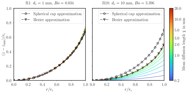
Figure 7 shows that the meniscus deepest point lies in the capillary center () in all simulated cases. The gradient for yielding a continuously differentiable surface for . Further, the water rises at the capillary walls () in both cases in order to meet the contact angle boundary condition. The meniscus shape where this boundary condition is satisfied, is referred to as fully developed shape in the following. This shape corresponds to the meniscus of a motionless fluid in a round capillary of infinite height. In the R10 case, the meniscus is not fully developed for , as visible in the right graph. In those simulations, the water surface reaches the top of the capillary which results in an increasing contact angle in order to comply with the volume conservation. However, in the R1 case, the meniscus is fully developed for all mean diffusion lengths due to the liquid elevation not being limited at the top of the capillary.
Differences in meniscus shape depend strongly on the Bond number which relates gravitational forces to surface tension forces. It is defined as for round capillaries where is the gravity constant. For capillaries with a sufficiently small diameter where , surface tension dominates the force balance at the interface which results in an approximate shape of a spherical cap [27, 28]. The surface formation simulation of the R1 case on the left side of Figure 7 shows only slight deviations from the spherical cap approximation.
However, for large diameters with , the spherical cap approximation fails to estimate the meniscus shape as shown in Figure 7 for the R10 case. This is due to the dominance of gravitational forces, which result in a flattened liquid surface at the center of the capillary [27]. Using the well-known Young-Laplace equation, an equation for the meniscus shape can be derived which also takes gravity effects into consideration. Lewis and Matsuura [27] proposed a method to approximate this equation using a Bezier curve approach.
Using the Bezier curve method, the meniscus shape in both cases is solved numerically with Python 3.10 and the SciPy 1.13.1 package [29]. Therefore, the trust-constr minimization algorithm [30, 31] is used to approximate the modified Young-Laplace equation and incorporate constraints, initial and boundary conditions. For both capillaries, the fully developed menisci in SE coincide with the Bezier approximation. Thus, SE accomplishes to approximate the Young-Laplace equation for fully developed menisci.
The R1 and R10 cases are used to validate the presented method and can be compared to the analytical solution from Stefan [2]. According to Stefan, the evaporation rate of round capillaries is calculated by
| (17) |
The analytical solution from Stefan does not consider an initial mass boundary layer over the capillary which leads to for . To take the initial mass boundary layer above the capillary into account, Camassel et al. [3] use a modified diffusion length where is the assumed uniform thickness of the external mass boundary layer. In order to better compare the analytical solution with the experimental results, the boundary layer thickness is calculated from the experimental data using the following equation by Camassel et al. [3]
| (18) |
The simulated results are compared with the experiments and the analytical solution in Figure 8.
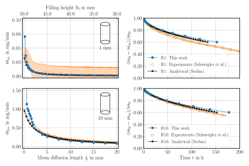
The left graphs in Figure 8 show the evaporation rate for the 1 and the 10 capillary. In both cases, the evaporation rate is highest for and decreases at higher mean diffusion lengths. In the R1 case, the simulated evaporation rate lies perfectly within the experimental error band for and further matches the analytical solution for . The simulated evaporation rate in the R10 case deviates more from the experiments in the beginning compared to the R1 case, but shows good agreement for nonetheless. Deviations in the beginning must not be caused by simulation errors but could also be attributed to small changes in the meniscus position at which the logging started in the experiments.
Although the proposed method provides reasonable results in most simulations, the evaporation rate for in the R10 case is exceptionally high. This can be traced back to a failed meshing process in sHM which occurs irregularly and is part of further improvement.
The simulations and the analytical solution in both cases predict a slower decrease of water mass on the long run compared to the experiments as depicted in the right graphs of Figure 8. This can be an indicator for additional effects that promote evaporation which are not considered in the analytical solution and the simulation. Further work should investigate the influence of buoyancy-driven convection on the evaporation rate, since temperature gradients in the experimental setup could induce currents that enhance the transport of water vapor out of the capillary.
3.2 Square capillaries
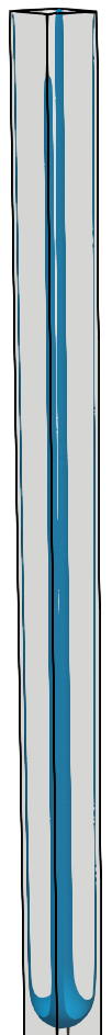
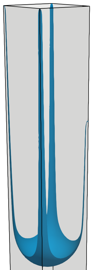
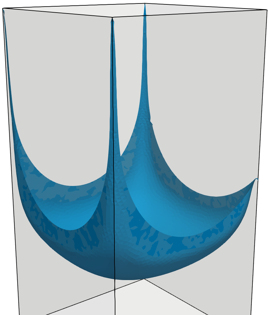
Previous experiments by Schweigler et al. [4] show that the evaporation rate increases significantly for capillaries with a square cross-section compared to round capillaries with a similar cross-sectional area. The reason for higher evaporation rates is the presence of liquid fingers in the corners of the capillary, resulting in a local reduction of the diffusion length [4]. In order to elaborate the influence of liquid fingers on the evaporation rate, simulations of square capillaries with an inner edge length of (cases S1, S4, S13) are performed. As a first step, the liquid surface formation is simulated in SE for the mean diffusion lengths in Equation 16. The resulting water surface for case S1 is shown as an example in Figure 9.
The water surfaces in Figure 9 are axisymmetric in relation to the capillary principal axis. For the specified geometry, the contact angle of does not satisfy Concus and Finn’s condition for a bounded solution of the Young-Laplace equation [7] which results in liquid fingers, rising inside the corners of the capillary. Based on investigations from Chauvet et al. [9], the liquid finger length strongly depends on the corner roundedness of the capillary. The investigated square capillary has sharp corners which in theory results in infinitely high finger lengths. Since the capillary height is limited in the simulation, the liquid fingers stop at the top of the capillary as depicted in Figure 9.
Figure 10 shows the cross-section of a single liquid finger for the S1, S4 and S13 case and various mean diffusion lengths. The liquid fingers are each cut at 25%, 50% and 75% of the total meniscus height which is the distance between the surfaces deepest and highest points.
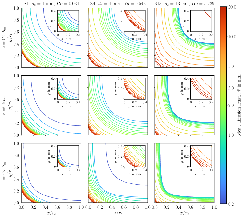
In order to comply with the contact angle boundary condition, the fingers are horizontally curved. For higher mean diffusion lengths, the fingers rise vertically in the corners and their thickness approaches a minimum value. Although the capillary widths between the S1 and S13 cases are an order of magnitude apart, the minimum finger thickness is in the same order of magnitude. Furthermore, the minimum finger thickness does not change significantly over the finger height. In the S1 case, the finger thickness quickly approaches a limit for small mean diffusion lengths, whereas in the S13 case, the fingers are developed at much higher mean diffusion lengths. Figure 10 also shows that the water surface in the S13 case tends to represent the outer square shape more strongly than the S1 case. This is attributed to the Bond number being higher, thus gravitational effects dominate capillary effects.
After simulating the water surface, the evaporation rate is determined according to Section 2.3. The simulative results and the experimental values are shown in Figure 11.
The total evaporation rate in the S1 case on the upper left of Figure 11 matches the experimental data well, although the simulated evaporation rates are slightly higher than the mean values from the experiment. However, the general trend of the experiment is well replicated.
In the S1 case, the measured water mass can be separated into three distinct phases that were previously described by Chauvet et al. [11] (see Section 1). The transition from CRP to FRP is characterized by a reduction in evaporation rate, attributed to the depinning of liquid fingers from the open end of the capillary. Given that the simulations are performed with sharp capillary corners, the natural depinning that occurs due to rounded corners cannot be replicated in the simulations.
In the S4 and S13 case, the simulation also overestimates the evaporation rate in the beginning but approaches the experimental values for increasing mean diffusion lengths. The deviations in the beginning only have a minor influence on the predicted water mass, as depicted in the right graphs. However, the evaporation rate in the S13 case is underestimated for which leads to a slower drying, compared to the experiment, as visualized in the lower right graph.
The previous observations show that the proposed method enables the determination of evaporation rate also for square capillaries. Expected liquid fingers could be verified in the simulations which lead to a higher evaporation rate compared to round capillaries. Due to the anti-proportional relation between time and evaporation rate (see Equation 2), minor deviations in evaporation rate result in slower drying compared to the experiment. This behavior is more pronounced in case of wide capillaries and can also be observed for the round capillaries which might be attributed to large scale effects, such as convection inside the capillary.
3.3 Temperature dependence
Previous simulations were only conducted for a temperature of C and a relative humidity of . In order to predict evaporation rates for different thermodynamical boundary conditions, only the vapor diffusion simulations are repeated for various temperatures while the relative humidity is kept constant. Simulations are conducted as an example for the S1 case from Section 3.2. Thermal influences on contact angle and surface tension are neglected, thus the same set of surfaces from SE is used for all investigated temperatures.
Since the temperature is not a direct input to the diffusion simulation, it must be used to determine the vapor mass fractions at the meniscus and environment, according to Equations 11, 12 and 13. In order to evaluate the evaporation rate, the gas mixture density and the diffusion coefficient in Equation 15 must be adapted. The calculated values are listed in Table 4 and the respective results are plotted in Figure 12.
| in ∘C | 10 | 20 | 23 | 30 | 40 | 50 | 60 | 70 | 80 | 90 |
|---|---|---|---|---|---|---|---|---|---|---|
| in % | 17 | 17 | 17 | 17 | 17 | 17 | 17 | 17 | 17 | 17 |
| in g/kg | 1.30 | 2.48 | 2.98 | 4.51 | 7.86 | 13.17 | 21.36 | 33.65 | 51.69 | 77.72 |
| in g/kg | 7.68 | 14.71 | 17.71 | 26.90 | 47.32 | 80.64 | 134.2 | 219.9 | 359.1 | 594.2 |
| in kg/m3 | 1.24 | 1.20 | 1.18 | 1.15 | 1.11 | 1.06 | 1.01 | 0.96 | 0.89 | 0.81 |
| in mm2/s | 22.88 | 24.31 | 24.75 | 25.78 | 27.28 | 28.83 | 30.41 | 32.02 | 33.67 | 35.36 |
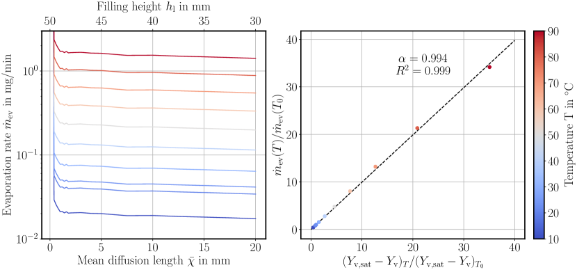
The results in Figure 12 on the left side show that the evaporation rate increases significantly with higher temperatures and that the graphs are self-similar to each other because the water surface has not been adjusted to account for temperature changes. In the logarithmic scale of the plot, the evaporation rate increases almost linear which allows the assumption of an exponential relation . In fact, the evaporation rate depends on the mass fraction gradient which is related to the temperature in terms of the Antoine Equation 11.
To obtain a general correlation for , the influence of the mass fraction difference on the evaporation rate is investigated. Therefore, the relationship
| (19) |
is proposed, with the proportionality factor . The proportionality factor is determined by normalizing all evaporation rates in Figure 12 using the evaporation rate at C. Further, the vapor mass fraction differences at each temperature are normalized by the vapor mass fraction difference at C. The resulting plot is depicted in Figure 12 on the right side.
The plot shows that the normalized evaporation rate strongly correlates with the vapor mass fraction ratio. The correlation factor is and the proportionality factor evaluates to . According to the simulative results the evaporation rate can be easily adapted to various temperatures, depending on the vapor mass fraction difference. This allows to simulate the evaporation rate only for one specific temperature and calculate the evaporation rate for a different temperature using Equation 19. Nevertheless, experiments with higher temperatures must be performed in the future, in order to validate the presented results and provide information, whether additional non-linear effects must be included in the simulation.
3.4 Runtime
The major advantage of the presented method is the short simulation runtime. All simulations were carried out on a high performance cluster that runs Linux and uses Intel Xeon Gold 6342 CPUs (Central Processing Unit). The simulation process is subdivided into four steps in order to set the computational resources according to the individual computational requirements. The respective steps and resources are listed in Table 5.
| Step | Description | No. of cores | Max. memory per core in GB |
|---|---|---|---|
| 1 | Surface formation simulation | 1 | 0.5 |
| 2 | Meshing preparation | 1 | 16 |
| 3 | Meshing (sHM) | 4 | 8 |
| 4 | Vapor diffusion simulation | 1 | 16 |
In the following, the first step is considered separately, since it only involves SE calculations while step 2,3 and 4 incorporate Linux commands and OF calculations. The runtime for all simulations from Sections 3.1 and 3.2 are visualized in Figure 13.
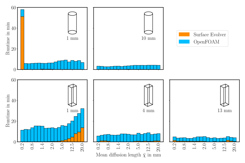
With the presented method we are now able to run simulations in 5 min to 60 min to cover up to 178 h of physical time for round capillaries. The simulation runtime is dominated by the calculations in OF while the SE runtime is negligible. Only in one case, the SE struggles to simulate the water surface for (see Figure 13 upper left) which is attributed to slow surface energy decrease. This behavior is likely caused by bad initial conditions for high filling heights as discussed in B and is part of further investigations.
The square capillary simulation runtime is between 5 min and 30 min and is also dominated by the OF simulations, although the SE runtime increases continuously for higher mean diffusion lengths in the S1 case. This is related to the formation of liquid fingers and their increasing height.
Although the simulated physical time ranges from in the S1 case to in the R10 case, the maximum runtime of the simulations is only . Since the simulations for various mean diffusion lengths are independent from each other, it must be emphasized that all simulations can run at the same time if sufficient CPUs are provided. To the best of our knowledge, there is no other method with a comparable runtime while still providing accurate results.
3.5 Generalization
Idealized geometries like round or square capillaries are rarely found in real-world applications. Nevertheless, rectangular gaps are often created by ribs that are used to increase stiffness of industrial housings. In order to test the proposed method for a wider range of applications, simulations are conducted for flat gaps with various length-to-width ratios. The gap width and height are kept constant at and respectively. The gap length is set according to a length-to-width ratio ranging from . The thermodynamical boundary conditions are . Using the presented method, the simulated evaporation rate and mass decrease over time are visualized in Figure 14.
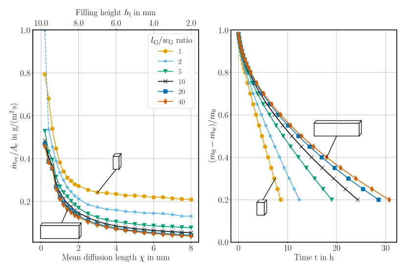
To better compare the evaporation rate in various gaps, the results are normalized by the cross-sectional area of the gap. The graph clearly shows that the normalized evaporation rate is highest for and decreases towards a limit for higher length-to-width ratios. As described in Section 3.2, the liquid finger thickness increases only slightly for higher capillary widths which results in a decreasing influence of liquid fingers for higher ratios. The mass plot allows for a similar conclusion, as the water volume and absolute evaporation rate depend linearly on the gap cross-sectional area. With the presented method, the evaporation in arbitrary capillaries can be simulated within a reasonable simulation time, as far as the geometry can be described in SE. Future work should focus on incorporating STL (stereolithography) files in SE and conducting experiments to validate the simulated results shown here.
4 Conclusion
This work presents a novel semi-transient simulation approach to estimate evaporation rates in small gaps, relevant to industrial applications. By decoupling the simulation of the liquid-gas interface from the vapor diffusion simulation, the approach addresses the challenges of long simulation times and numerical errors associated with traditional methods like Volume-of-Fluid. The proposed method utilizes SE to simulate the fluid surface formation, considering capillary effects and then employs OF to simulate vapor diffusion in the gas domain. The source code is uploaded to the Bosch Research GitHub 222https://github.com/boschresearch/sepMultiphaseFoam/tree/publications/novelSimulationApproachForEvaporationProcesses. The decoupling allows for the evaporation rate to be calculated independently of previous time steps, enabling highly parallelized simulations.
The key advantage of this method is its speed. Simulations for round, square and rectangular capillaries were conducted, covering physical times up to 178 hours, that are completed within 1 hour of computational time. The simulations significantly outperform conventional methods like Volume-of-Fluid, which require small time steps to resolve the interface motion coupled with evaporation, resulting in prohibitively long simulation times for realistic scenarios.
The numerical investigations conducted for round and square capillaries demonstrate good agreement with experimental results for a wide range of capillary sizes. While the approach effectively predicts liquid finger formation in square and rectangular capillaries and captures the associated increase in evaporation rate, some limitations were observed. In narrow capillaries with large filling heights, the accurate prediction of the liquid surface and the evaporation rate becomes more challenging, leading to deviations from experimental values. Simulations were also conducted for gaps, showing the wide applicability of this method. The simulation runtime remains significantly lower than fully coupled approaches, highlighting the computational efficiency of the proposed method.
Future work will focus on incorporating the influence of corner roundedness in square capillaries to include the prediction of depinning and the associated phases which were described by Chauvet et al. [9]. Furthermore, the inclusion of buoyancy-driven convection, could enhance the model’s accuracy and applicability to more complex scenarios. Experimental validation for a broader range of geometries will also be pursued to further refine the proposed method. This novel approach provides a valuable tool to understand and predict evaporation processes, contributing to improved product design and corrosion mitigation in industrial applications.
Appendix A Surface Evolver parameter settings
As described in Section 2, the SE simulates the liquid surface based on a gradient descent approach. Therefore, a velocity vector is calculated for each vertex, based on the contribution of a vertex to the minimization of the total surface energy [22]. In each iteration a vertex is moved along the velocity vector according to
| (20) |
where is the vertex position and is a universal scale factor that can be interpreted as a learning rate or time step for the algorithm [22]. In order to increase convergence speed, the scale factor is optimized each iteration, whereas is limited to by default. Although this setting yields good results for low mean diffusion lengths, artificial depinning of liquid fingers in the corners of square capillaries can be observed for high mean diffusion lengths, as shown in Figure 15.
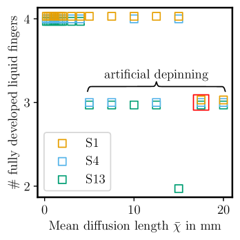
In the investigated cases, the artificial depinning is only observed for high mean diffusion lengths and tends to occur more often in cases where the liquid finger thickness is small in relation to the capillary cross-sectional area. For the investigated cases and mean diffusion lengths the number of liquid fingers that rise to the top of the capillary is plotted in Figure 15 on the right side. In the S1 case, only the simulations for have less than 4 fingers whereas the artificial depinning occurs irregularly for in the S4 and S13 case. According to the diagram in Figure 15, the investigated simulations show no clear dependency on the mean diffusion length at which all liquid fingers are no longer fully developed.
To calculate the velocity vector of a vertex, the surface energy gradient is multiplied with the surface tension. The surface tension of water is in the order of which results in a velocity vector of similar order of magnitude. This leads to the vertices moving too little to reach a global energy minimum state, thus a local minimum is found which incorporates depinned liquid fingers. This behavior can be prevented by using a scale limit of [22]. By scaling the velocity vector with the inverse of the surface tension, the velocity vector is guaranteed to be in the order of and allows the gradient descent approach to find the global minimum rather than a local minimum. A scale limit of is used throughout this work which solves the problem of artificial depinning.
Appendix B Reliability
The method presented in this paper allows the user to simulate evaporation from small cavities in a very fast way. However, it also has some limitations. SE has a particularly difficult time finding a steady-state solution in rare cases (see Section 3.4), if the initial surface is close to the top of the capillary.
Usually the initialized water surface does not meet the contact angle boundary condition, thus the initial water surface will be far away from a fully developed state. This results in high surface energy gradients in the first iterations that further lead to large vertex movement , since in Equation 20. Large vertex movements are particularly detrimental if the initialized surface is close to the top of the capillary. This leads to the velocity vector moving vertices outside the prescribed geometry, as shown in Figure 16(a), which triggers instabilities and results in unreasonable surfaces (see Figures 16(b) and 16(c)).


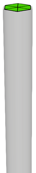
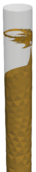
In Figure 16, the surfaces are initialized at followed by a different amount of refinement and iteration steps. Figure 16(b) shows the result for a capillary without an explicit upper boundary condition where is the vertices z coordinate. After the first iteration step, the surface already diverges and breaks out of the capillary. Further iterations lead to a stable solution above the capillary although the volume conservation is violated. Numerical errors result in liquid droplets above the actual liquid surface.
Figure 16(c) shows the resulting surface with an explicitly implemented upper surface boundary condition . In the first iteration the vertices are projected to the upper boundary, demonstrating the conditions effectiveness. However, the convergence algorithm leads to a very distorted and unreasonable surface.
To obtain reasonable results, the relation , where is the minimum edge length at a vertex, is used to reduce the magnitude of the velocity vector at the start of a simulation. Therefore, each initial surface is refined, followed by SE iteration steps before starting the actual SE-FIT convergence algorithm. Three refinement steps, followed by 100 SE iterations showed the best results, as visualized in Figure 16(d), and is therefore used throughout this work.
References
-
[1]
N. Kubochkin, T. Gambaryan-Roisman, Capillary-driven flow in corner geometries, Current Opinion in Colloid & Interface Science 59 (2022) 101575.
doi:10.1016/j.cocis.2022.101575.
URL https://linkinghub.elsevier.com/retrieve/pii/S1359029422000140 - [2] J. Stefan, Über das Gleichgewicht und die Bewegung, insbesondere die Diffusion von Gasgemengen, Sitzungsberichte der Mathematisch-Naturwissenschaftlichen Classe der Kaiserlichen Akademie der Wissenschaften Wien, 2te Abteilung 63 (1871) 63 – 124.
-
[3]
B. Camassel, N. Sghaier, M. Prat, S. Ben Nasrallah, Evaporation in a capillary tube of square cross-section: application to ion transport, Chemical Engineering Science 60 (3) (2005) 815–826.
doi:10.1016/j.ces.2004.09.044.
URL https://linkinghub.elsevier.com/retrieve/pii/S0009250904007043 -
[4]
K. Schweigler, S. Seifritz, M. Selzer, B. Nestler, Evaporation rate analysis of capillaries with polygonal cross-section, International Journal of Heat and Mass Transfer 121 (2018) 943–951.
doi:10.1016/j.ijheatmasstransfer.2017.12.090.
URL https://linkinghub.elsevier.com/retrieve/pii/S0017931017344241 -
[5]
R. S. G. Britain), Philosophical Transactions of the Royal Society of London, no. Bd. 95, W. Bowyer and J. Nichols for Lockyer Davis, printer to the Royal Society, 1805.
URL https://books.google.de/books?id=C5JJAAAAYAAJ -
[6]
P. de Laplace, J. Duprat, Traité de mécanique céleste /par P.S. Laplace … ; tome premier [-quatrieme], no. Bd. 4 in Traité de mécanique céleste /par P.S. Laplace … ; tome premier [-quatrieme], de l’Imprimerie de Crapelet, 1805.
URL https://books.google.de/books?id=_A8OAAAAQAAJ -
[7]
P. Concus, R. Finn, ON THE BEHAVIOR OF A CAPILLARY SURFACE IN A WEDGE, Proceedings of the National Academy of Sciences 63 (2) (1969) 292–299.
doi:10.1073/pnas.63.2.292.
URL https://pnas.org/doi/full/10.1073/pnas.63.2.292 -
[8]
T. Ransohoff, C. Radke, Laminar flow of a wetting liquid along the corners of a predominantly gas-occupied noncircular pore, Journal of Colloid and Interface Science 121 (2) (1988) 392–401.
doi:10.1016/0021-9797(88)90442-0.
URL https://linkinghub.elsevier.com/retrieve/pii/0021979788904420 -
[9]
F. Chauvet, P. Duru, M. Prat, Depinning of evaporating liquid films in square capillary tubes: Influence of corners’ roundedness, Physics of Fluids 22 (11) (2010) 112113.
doi:10.1063/1.3503925.
URL https://pubs.aip.org/pof/article/22/11/112113/1013834/Depinning-of-evaporating-liquid-films-in-square -
[10]
E. Keita, S. A. Koehler, P. Faure, D. A. Weitz, P. Coussot, Drying kinetics driven by the shape of the air/water interface in a capillary channel, The European Physical Journal E 39 (2) (2016) 23.
doi:10.1140/epje/i2016-16023-8.
URL http://link.springer.com/10.1140/epje/i2016-16023-8 -
[11]
F. Chauvet, P. Duru, S. Geoffroy, M. Prat, Three Periods of Drying of a Single Square Capillary Tube, Physical Review Letters 103 (12) (2009) 124502.
doi:10.1103/PhysRevLett.103.124502.
URL https://link.aps.org/doi/10.1103/PhysRevLett.103.124502 -
[12]
A. G. Yiotis, D. Salin, E. S. Tajer, Y. C. Yortsos, Analytical solutions of drying in porous media for gravity-stabilized fronts, Physical Review E 85 (4) (2012) 046308.
doi:10.1103/PhysRevE.85.046308.
URL https://link.aps.org/doi/10.1103/PhysRevE.85.046308 -
[13]
N. Scapin, P. Costa, L. Brandt, A volume-of-fluid method for interface-resolved simulations of phase-changing two-fluid flows, Journal of Computational Physics 407 (2020) 109251.
doi:10.1016/j.jcp.2020.109251.
URL https://linkinghub.elsevier.com/retrieve/pii/S0021999120300255 -
[14]
S. Hardt, F. Wondra, Evaporation model for interfacial flows based on a continuum-field representation of the source terms, Journal of Computational Physics 227 (11) (2008) 5871–5895.
doi:10.1016/j.jcp.2008.02.020.
URL https://linkinghub.elsevier.com/retrieve/pii/S0021999108001228 -
[15]
M. Irfan, M. Muradoglu, A front tracking method for direct numerical simulation of evaporation process in a multiphase system, Journal of Computational Physics 337 (2017) 132–153.
doi:10.1016/j.jcp.2017.02.036.
URL https://linkinghub.elsevier.com/retrieve/pii/S0021999117301304 -
[16]
M. N. Farooqi, D. Izbassarov, M. Muradoğlu, D. Unat, Communication analysis and optimization of 3D front tracking method for multiphase flow simulations, The International Journal of High Performance Computing Applications 33 (1) (2019) 67–80.
doi:10.1177/1094342017694426.
URL http://journals.sagepub.com/doi/10.1177/1094342017694426 -
[17]
J. Schlottke, B. Weigand, Direct numerical simulation of evaporating droplets, Journal of Computational Physics 227 (10) (2008) 5215–5237.
doi:10.1016/j.jcp.2008.01.042.
URL https://linkinghub.elsevier.com/retrieve/pii/S0021999108000740 -
[18]
J. Palmore, O. Desjardins, A volume of fluid framework for interface-resolved simulations of vaporizing liquid-gas flows, Journal of Computational Physics 399 (2019) 108954.
doi:10.1016/j.jcp.2019.108954.
URL https://linkinghub.elsevier.com/retrieve/pii/S002199911930659X - [19] K. M. Schweigler, Analyse geometrieabha\”ngiger Verdunstungsraten in ungesa\”ttigter, konvektionsfreier Atmospha\”re, PhD Thesis, Karlsruher Institut für Technologie (KIT) (2017). doi:10.5445/IR/1000077924.
-
[20]
E. Sultan, A. Boudaoud, M. Ben Amar, Evaporation of a thin film: diffusion of the vapour and Marangoni instabilities (Aug. 2004).
URL https://hal.science/hal-00002706 - [21] K. A. Brakke, The surface evolver, Experimental Mathematics 1 (2) (1992) 141 – 165, publisher: A K Peters, Ltd.
-
[22]
K. Brakke, Surface Evolver (Aug. 2013).
URL https://kenbrakke.com/evolver/evolver.html -
[23]
Y. Chen, B. Schaffer, M. Weislogel, G. Zimmerli, Introducing SE-FIT: Surface Evolver - Fluid Interface Tool for Studying Capillary Surfaces, in: 49th AIAA Aerospace Sciences Meeting including the New Horizons Forum and Aerospace Exposition, American Institute of Aeronautics and Astronautics, Orlando, Florida, 2011.
doi:10.2514/6.2011-1319.
URL https://arc.aiaa.org/doi/10.2514/6.2011-1319 -
[24]
E. N. Fuller, K. Ensley, J. C. Giddings, Diffusion of halogenated hydrocarbons in helium. The effect of structure on collision cross sections, The Journal of Physical Chemistry 73 (11) (1969) 3679–3685.
doi:10.1021/j100845a020.
URL https://pubs.acs.org/doi/abs/10.1021/j100845a020 -
[25]
VDI e. V. (Ed.), VDI-Wärmeatlas, Springer Berlin Heidelberg, Berlin, Heidelberg, 2013.
doi:10.1007/978-3-642-19981-3.
URL http://link.springer.com/10.1007/978-3-642-19981-3 - [26] R. C. Reid, J. M. Prausnitz, B. E. Poling, The properties of gases and liquids, 4th Edition, McGraw-Hill, New York, 1987.
-
[27]
K. Lewis, T. Matsuura, Calculation of the Meniscus Shape Formed under Gravitational Force by Solving the Young–Laplace Differential Equation Using the Bézier Curve Method, ACS Omega 7 (41) (2022) 36510–36518.
doi:10.1021/acsomega.2c04359.
URL https://pubs.acs.org/doi/10.1021/acsomega.2c04359 -
[28]
D. Gründing, M. Fricke, D. Bothe, Capillary Rise ‐ Jurin’s Height vs Spherical Cap, PAMM 19 (1) (2019) e201900336.
doi:10.1002/pamm.201900336.
URL https://onlinelibrary.wiley.com/doi/10.1002/pamm.201900336 -
[29]
P. Virtanen, R. Gommers, T. E. Oliphant, M. Haberland, T. Reddy, D. Cournapeau, E. Burovski, P. Peterson, W. Weckesser, J. Bright, S. J. van der Walt, M. Brett, J. Wilson, K. J. Millman, N. Mayorov, A. R. J. Nelson, E. Jones, R. Kern, E. Larson, C. J. Carey, I. Polat, Y. Feng, E. W. Moore, J. VanderPlas, D. Laxalde, J. Perktold, R. Cimrman, I. Henriksen, E. A. Quintero, C. R. Harris, A. M. Archibald, A. H. Ribeiro, F. Pedregosa, P. van Mulbregt, SciPy 1.0 Contributors, A. Vijaykumar, A. P. Bardelli, A. Rothberg, A. Hilboll, A. Kloeckner, A. Scopatz, A. Lee, A. Rokem, C. N. Woods, C. Fulton, C. Masson, C. Häggström, C. Fitzgerald, D. A. Nicholson, D. R. Hagen, D. V. Pasechnik, E. Olivetti, E. Martin, E. Wieser, F. Silva, F. Lenders, F. Wilhelm, G. Young, G. A. Price, G.-L. Ingold, G. E. Allen, G. R. Lee, H. Audren, I. Probst, J. P. Dietrich, J. Silterra, J. T. Webber, J. Slavič, J. Nothman, J. Buchner, J. Kulick, J. L. Schönberger, J. V. de Miranda Cardoso, J. Reimer, J. Harrington, J. L. C. Rodríguez,
J. Nunez-Iglesias, J. Kuczynski, K. Tritz, M. Thoma, M. Newville, M. Kümmerer, M. Bolingbroke, M. Tartre, M. Pak, N. J. Smith, N. Nowaczyk, N. Shebanov, O. Pavlyk, P. A. Brodtkorb, P. Lee, R. T. McGibbon, R. Feldbauer, S. Lewis, S. Tygier, S. Sievert, S. Vigna, S. Peterson, S. More, T. Pudlik, T. Oshima, T. J. Pingel, T. P. Robitaille, T. Spura, T. R. Jones, T. Cera, T. Leslie, T. Zito, T. Krauss, U. Upadhyay, Y. O. Halchenko, Y. Vázquez-Baeza, SciPy 1.0: fundamental algorithms for scientific computing in Python, Nature Methods 17 (3) (2020) 261–272.
doi:10.1038/s41592-019-0686-2.
URL https://www.nature.com/articles/s41592-019-0686-2 - [30] J. Nocedal, S. J. Wright, Numerical optimization, 2nd Edition, Springer series in operations research, Springer, New York, 2006, oCLC: ocm68629100.
-
[31]
M. Lalee, J. Nocedal, T. Plantenga, On the Implementation of an Algorithm for Large-Scale Equality Constrained Optimization, SIAM Journal on Optimization 8 (3) (1998) 682–706.
doi:10.1137/S1052623493262993.
URL http://epubs.siam.org/doi/10.1137/S1052623493262993