Estimating shared subspace with AJIVE:
the power and limitation of multiple data matrices

Abstract

Integrative data analysis often requires disentangling joint and individual variations across multiple datasets, a challenge commonly addressed by the Joint and Individual Variation Explained (JIVE) model. While numerous methods have been developed to estimate the shared subspace under JIVE, the theoretical understanding of their performance remains limited, particularly in the context of multiple matrices and varying levels of subspace misalignment. This paper bridges this gap by providing a systematic analysis of shared subspace estimation in multi-matrix settings.

We focus on the Angle-based Joint and Individual Variation Explained (AJIVE) method, a two-stage spectral approach, and establish new performance guarantees that uncover its strengths and limitations. Specifically, we show that in high signal-to-noise ratio (SNR) regimes, AJIVE’s estimation error decreases with the number of matrices, demonstrating the power of multi-matrix integration. Conversely, in low-SNR settings, AJIVE exhibits a non-diminishing error, highlighting fundamental limitations. To complement these results, we derive minimax lower bounds, showing that AJIVE achieves optimal rates in high-SNR regimes. Furthermore, we analyze an oracle-aided spectral estimator to demonstrate that the non-diminishing error in low-SNR scenarios is a fundamental barrier. Extensive numerical experiments corroborate our theoretical findings, providing insights into the interplay between SNR, matrix count, and subspace misalignment.

1 Introduction

Modern data analysis is increasingly focused on integrating information from multiple sources. This has sparked a wave of applications using diverse datasets, such as identifying communities within heterogeneous networks [MLZ22], analyzing various types of high-dimensional genomic data [LHMN13], and discerning global and local features in federated learning [SK24]. A significant challenge in these analyses lies in separating the joint and individual variations present in such multi-view datasets.

In the seminal paper [LHMN13], Lock et al. pioneered a matrix decomposition model known as Joint and Individual Variation Explained (JIVE). JIVE models each dataset as a noisy low-rank matrix $\bm{A}_{k}\in\mathbb{R}^{n\times d_{k}}$, which can be further decomposed into

$$\bm{A}_{k}\approx\bm{U}^{\star}\bm{V}_{k}^{\star\top}+\bm{U}_{k}^{\star}\bm{W}_{k}^{\star\top}\in\mathbb{R}^{n\times d_{k}},\qquad\text{for }1\leq k\leq K.$$ (1)

Here, $\bm{U}^{\star}$—an $n\times r$ orthonormal matrix, denotes the shared subspace, and $\bm{U}_{k}^{\star}\perp\bm{U}^{\star}$—an $n\times r_{k}$ orthonormal matrix, denotes the unique subspace. In words, JIVE assumes that the column spaces of multiple data matrices share the same component $\mathrm{col}(\bm{U}^{\star})$, while each matrix also has a unique subspace modeled by $\mathrm{col}(\bm{U}_{k}^{\star})$.

Despite its wide adoption and various methodological advancements, the theoretical understanding of shared subspace estimation under the JIVE model remains limited compared to single-matrix subspace estimation [CLC⁺21]. Two key challenges contribute to this gap:

• Impact of multiple matrices. Theoretical studies on shared subspace estimation often focus on cases with only two matrices (see e.g., [STG24, MM24]), leaving the potential advantages and limitations of having multiple matrices unexplored.

• Impact of unique subspaces. The identifiability of the model requires that the unique subspaces $\{\mathrm{col}(\bm{U}_{k}^{\star})\}$ do not have an intersection, i.e., they are misaligned. Conceptually, estimating the shared subspace becomes more challenging when the unique subspaces are less misaligned. Existing work [ZT22, MM24] typically assumes highly misaligned subspaces, overlooking a broader spectrum of alignment scenarios.

Our contributions.

In this work, we establish fundamental limits for estimating shared subspaces from multiple matrices, highlighting dependencies on the signal-to-noise ratio (SNR), the number of matrices, and the degree of subspace misalignment. Key results include:

• Performance guarantees for AJIVE: We derive new statistical guarantees for AJIVE, a two-stage spectral method [FJHM18]. These results reveal that (1) in high-SNR regimes, estimation error decreases with more matrices, demonstrating the benefits of multi-matrix integration, and (2) in low-SNR regimes, AJIVE’s error does not diminish even as the number of matrices grows, illustrating inherent limitations.

• Minimax lower bounds: We prove that AJIVE achieves optimal performance in high-SNR settings, confirming its efficiency. More importantly, the optimal rate of convergence is faster when the level of misalignment is lower, confirming our intuition.

• Insights into low-SNR limitations: Numerical experiments corroborate our theoretical findings, showing that AJIVE’s error stagnation is not merely an artifact of analysis but a fundamental barrier. Furthermore, we provide lower bounds for an oracle-aided spectral estimator, establishing that non-diminishing error persists even under ideal conditions.

By addressing these challenges, our work offers a deeper understanding of shared subspace estimation and the role of multiple matrices in integrative data analysis.

1.1 Related work

JIVE.

The JIVE model is originally proposed in the paper [LHMN13], in which they also propose a nonconvex least-squares approach to estimate the shared and indivual components. A similar approach is discussed in the work [ZCZM15]. The optimization-based approach is iterative and computationally intensive. As a remedy, Feng et al. [FJHM18] proposed a two-stage spectral method AJIVE, followed by its robust version RaJIVE [PTG21]. Other spectral approaches include stacked singular value decomposition (SVD) [MM24], and methods based on the product of projection matrices [STG24].

Instead of complete noisy observations, recent work [SKF23, SFAK24] has extended the JIVE model to accommodate missing data as well as entrywise outliers in the observed matrices.

When the matrices $\bm{V}^{\star}_{k}$ and $\bm{W}^{\star}_{k}$, the JIVE model is closely related to the personalized PCA problem [SKF23]. When there is no personalization, i.e., the unique components are not present, this problem reduces to the distributed PCA problem studied in [FWWZ19, ZT22].

In the JIVE model, the subspace $\mathrm{col}(\bm{U}^{\star})$ is assumed to be shared among all data matrices. Recent efforts have been made towards partially-shared subspaces, meaning that different subsets of the data matrices share different subspaces. Examples include Data Integraton via Anlysis of Subspaces (DIVAS) [PJH⁺24], covariate-driven factorization by thresholding for multiblock data [GLLJ21], and Structural Learning and Integrative DEcomposition of multi-view data (SLIDE)[GL19].

Subspace estimation from a single matrix.

Our theoretical investigation is closely related to estimating the subspace of a single matrix. Wedin’s theorem [Wed73], a classical result in matrix perturbation theory allows one to obtain perturbation bounds for both the left and right singular subspaces. However, the bound provided by Wedin is loose when we focus exclusively on column subspace estimation and the number of columns is much larger than the number of rows. The paper [CZ18] provides rate-optimal guarantees in this scenario. Later, Cai et al. [CLC⁺21] provides more refined analysis for subspace estimation in the face of missing data. We refer interested readers to the recent monograph on this topic [CCFM21].

Notation

For a positive integer $n$, we denote $[n]=\{1,2,\ldots,n\}$. For any $a,b\in\mathbb{R}$, $a\wedge b$ means the minimum of $a,b$, and $a\vee b$ means the maximum of $a,b$. For symmetric matrices $\bm{A},\bm{B}\in\mathbb{R}^{n\times n}$, $\bm{A}\preceq\bm{B}$ means $\bm{B}-\bm{A}$ is positive semidefinite, i.e., $\bm{v}^{\top}(\bm{B}-\bm{A})\bm{v}\geq 0$ for any $\bm{v}\in\mathbb{R}^{n}$. We use $\bm{e}_{i}$ to denote the standard unit vector with $1$ at $i$-th coordinate and 0 elsewhere. For any rank-$r$ matrix $\bm{A}$, we use $\sigma_{1}(\bm{A})\geq\sigma_{2}(\bm{A})\geq\ldots\geq\sigma_{r}(\bm{A})>0$ to denote its singular values. For any $n\times d$ matrix $\bm{A}$, we use $[\bm{A}]_{i,\cdot}$ to denote its $i$-th row in the form of a $1\times d$ matrix. We use $\mathrm{Trace}(\cdot)$ to denote the trace of a square matrix. For $r\leq d$, we use $\mathcal{O}^{d\times r}$ to denote the set of orthonormal matrices $\bm{U}$, i.e., $\bm{U}^{\top}\bm{U}=\bm{I}_{r}$. We use the big-O notation $O(X)$ to indicate any term $Y$ such that $Y\leq CX$ for some large enough constant $C$.

2 Background

In this section, we introduce the problem of estimating the shared subspace from multiple noisy data matrices, focusing on its identifiability. We also provide a review of the AJIVE method, a two-stage spectral method for shared subspace estimation.

2.1 Observation models

Consider $K$ ground truth matrices $\{\bm{A}_{k}^{\star}\}_{1\leq k\leq K}$, each with a low-rank decomposition

$$\bm{A}_{k}^{\star}=\bm{U}^{\star}\bm{V}_{k}^{\star\top}+\bm{U}_{k}^{\star}\bm{W}_{k}^{\star\top}\in\mathbb{R}^{n\times d_{k}}.$$ (2)

Here, $\bm{U}^{\star}\in\mathcal{O}^{n\times r}$ represents the shared subspace common to all matrices, and $\bm{U}_{k}^{\star}\in\mathcal{O}^{n\times r_{k}}\perp\bm{U}^{\star}$ represents the unique subspace specific to the $k$-th matrix. For each $k\in[K]$, $\bm{V}_{k}^{\star}\in\mathbb{R}^{d_{k}\times r}$ and $\bm{W}_{k}^{\star}\in\mathbb{R}^{d_{k}\times r_{k}}$ are full-rank loading matrices. Suppose we observe noisy versions of $\{\bm{A}_{k}^{\star}\}_{1\leq k\leq K}$:

$$\bm{A}_{k}=\bm{A}_{k}^{\star}+\bm{E}_{k},$$ (3)

where $\bm{E}_{k}$ denotes additive noise, containing i.i.d. Gaussian entries with mean 0 and variance $\sigma^{2}$. The goal is then to estimate the shared subspace $\bm{U}^{\star}$ based on noisy observations $\{\bm{A}_{k}\}_{1\leq k\leq K}$.

2.2 Identifiability of the shared subspace

Before discussing estimation methods, we must ensure that the shared subspace $\mathrm{col}(\bm{U}^{\star})$ is identifiable from the noiseless matrices $\{\bm{A}_{k}^{\star}\}$. The identifiability condition requires:

$$\mathrm{col}(\bm{U}^{\star})=\cap_{1\leq k\leq K}\mathrm{col}(\bm{A}_{k}^{\star}).$$ (4)

Note that the orthogonality constraint $\bm{U}_{k}^{\star}\perp\bm{U}^{\star}$ alone does not guarantee the identifiability condition (4). Additional assumptions are needed.

Faithfulness: $\mathrm{col}(\bm{U}^{\star})\subseteq\cap_{1\leq k\leq K}\mathrm{col}(\bm{A}_{k}^{\star})$.

Since we are estimating the shared subspace $\mathrm{col}(\bm{U}^{\star})$ among $\mathrm{col}(\bm{A}_{k}^{\star})$, it is necessary to assume that $\mathrm{col}(\bm{U}^{\star})\subseteq\mathrm{col}(\bm{A}_{k}^{\star})$. This together with the orthogonality constraint $\bm{U}^{\star}\perp\bm{U}_{k}^{\star}$ also implies $\mathrm{col}(\bm{U}_{k}^{\star})\subseteq\mathrm{col}(\bm{A}_{k}^{\star})$. In fact, both assumptions combined are equivalent to assuming $\mathrm{rank}(\bm{A}_{k}^{\star})=r+r_{k}$.

Throughout the paper, we define $\sigma_{\min}\coloneqq\min_{k}\sigma_{r+r_{k}}(\bm{A}_{k}^{\star})$, $\sigma_{\max}\coloneqq\max_{k}\sigma_{1}(\bm{A}_{k}^{\star})$ and the condition number to be $\kappa\coloneqq\sigma_{\max}/\sigma_{\min}$.

Exhaustiveness: $\cap_{1\leq k\leq K}\mathrm{col}(\bm{A}_{k}^{\star})\subseteq\mathrm{col}(\bm{U}^{\star}).$

Faithfulness of $\mathrm{col}(\bm{U}^{\star})$ allows us to conclude that $\mathrm{col}(\bm{U}^{\star})\subseteq\cap_{1\leq k\leq K}\mathrm{col}(\bm{A}_{k}^{\star})$. However, to enable identifiability, we still need to guarantee that $\cap_{1\leq k\leq K}\mathrm{col}(\bm{A}_{k}^{\star})\subseteq\mathrm{col}(\bm{U}^{\star})$, that is $\mathrm{col}(\bm{U}^{\star})$ includes all shared information in $\cap_{1\leq k\leq K}\mathrm{col}(\bm{A}_{k}^{\star})$. To illustrate potential issues, consider the degenerate case where $\cap_{1\leq k\leq K}\mathrm{col}(\bm{U}_{k}^{\star})\neq\emptyset$. In other words, there exists a common direction in the unique components. It is clear that $\mathrm{col}(\bm{U}^{\star})$ is a strict subset of $\cap_{1\leq k\leq K}\mathrm{col}(\bm{A}_{k}^{\star})$, and hence not identifiable. Consequently, to ensure identifiability, one needs to assume that $\cap_{1\leq k\leq K}\mathrm{col}(\bm{U}_{k}^{\star})=\emptyset$, i.e., the unique subspaces are misaligned.

In this paper, we quantify the level of misalignment among the unique subspaces via the following definition [SK24, SKF23].

Definition 1.

(misalignment) We say that the collection of subspaces $\{\bm{U}_{k}^{\star}\}$ is $\theta$-misaligned if

$$\left\|\frac{1}{K}\sum_{k=1}^{K}\bm{U}_{k}^{\star}\bm{U}_{k}^{\star\top}\right\|\leq 1-\theta.$$

It is easy to see that $\theta\in[0,1-1/K]$. We single out several interesting scenarios.

• Aligned. One of the extreme cases is when $\theta=0$. This is equivalent to $\cap_{1\leq k\leq K}\mathrm{col}(\bm{U}_{k}^{\star})\neq\emptyset$, i.e., the unique subspaces are aligned. In this case, the shared subspace is not identifiable.

• Misaligned. The other extreme case is when all the unique subspaces are orthogonal to each other, implying that $\left\|\frac{1}{K}\sum_{k=1}^{K}\bm{U}_{k}^{\star}\bm{U}_{k}^{\star\top}\right\|=1/K$, and that $\theta=1-1/K$. This is also the regime considered in the recent work [MM24].

• Realizability via randomization. Fix any $\theta\in(0,1-1/K]$. One can generate a collection of $\theta$-misaligned subspaces $\{\bm{U}_{k}^{\star}\}$ in a random fashion. To see this, for each $k\in[K]$, generate $\bm{U}_{k}^{\star}$ via

  $$\bm{U}_{k}^{\star}=\sqrt{1-\theta}\bm{Z}+\sqrt{\theta}\bm{Z}_{k}$$ (5)

  for some fixed $\bm{Z}\in\mathcal{O}^{d\times r_{k}}$, and $\bm{Z_{k}}\in\mathcal{O}^{d\times r_{k}}$ drawn uniformly at random from the orthogonal subspace to $\bm{Z}$. Rough calculations show that

  $$\left\|\frac{1}{K}\sum_{k=1}^{K}\bm{U}_{k}^{\star}\bm{U}_{k}^{\star\top}\right\|\approx\left\|\mathbb{E}\frac{1}{K}\sum_{k=1}^{K}\bm{U}_{k}^{\star}\bm{U}_{k}^{\star\top}\right\|=1-\theta.$$

2.3 Angle-based joint and individual variation explained (AJIVE)

Now we are ready to review the AJIVE method put forward in the paper [FJHM18] for extracting the shared and unique subspaces from noisy observations $\{\bm{A}_{k}\}$. AJIVE is essentially a two-stage spectral method. In the first stage, for each $k\in[K]$, we estimate the ($r+r_{k}$)-dimensional column space of $\bm{A}_{k}^{\star}$ using SVD of the noisy matrix $\bm{A}_{k}$. Then in the second stage, we combine the estimates in the first stage and use SVD again to estimate the most prominent (i.e., shared) $r$-dimensional subspace $\mathrm{col}(\bm{U}^{\star})$. See Algorithm 1 for the detailed descriptions of AJIVE.

Algorithm 1 Angle-based joint and individual variation explained (AJIVE)

Input: $\{\bm{A}_{k}\}_{k=1}^{K},r,\{r_{k}\}_{k=1}^{K}$.

1. For $k=1,\ldots,K$, Let $\widetilde{\bm{U}}_{k}$ be the top-$(r+r_{k})$ left singular matrix of $\bm{A}_{k}$.

2. Let $\widehat{\bm{U}}$ be the matrix whose columns are the top-$r$ eigenvectors of $\sum_{k=1}^{K}\widetilde{\bm{U}}_{k}\widetilde{\bm{U}}_{k}^{\top}$. Output $\mathrm{col}(\widehat{\bm{U}})$ as the estimate of $\mathrm{col}(\bm{U}^{\star})$.

3. (Optional) For $k=1,\ldots,K$, let $\widehat{\bm{V}}_{k}=\bm{A}_{k}^{\top}\widehat{\bm{U}}$, $\widehat{\bm{U}}_{k}$ be the top-$r_{k}$ left singular matrix of $\bm{I}_{n}-\widehat{\bm{U}}\widehat{\bm{V}}_{k}^{\top}$, and $\widehat{\bm{W}}_{k}=\bm{A}_{k}^{\top}\widehat{\bm{U}}_{k}$. Output $\widehat{\bm{V}}_{k},\widehat{\bm{U}}_{k},\widehat{\bm{W}}_{k}$ as the estimates of $\bm{V}_{k}^{\star},\bm{U}_{k}^{\star},\bm{W}_{k}^{\star}$, and

   $$\widehat{\bm{A}}_{k}\coloneqq\widehat{\bm{U}}\widehat{\bm{V}}_{k}^{\top}+\widehat{\bm{U}}_{k}\widehat{\bm{W}}_{k}^{\top}$$

   as the estimates of $\bm{A}_{k}^{\star}$.

AJIVE is one-shot, and hence computationally cheaper than other optimization-based methods [LHMN13]. In addition, it can be naturally distributed, and therefore can be made private.

A digression: failure of stacked SVD.

Another method to estimate the shared column space is to use the top eigenvectors of $\sum_{k=1}^{K}\bm{A}_{k}\bm{A}_{k}^{\top}$. This is equivalent to taking the left singular vectors of the stacked matrix $\begin{bmatrix}\bm{A}_{1}\cdots\bm{A}_{K}\end{bmatrix}$.

Stacked SVD is extensively studied in the concurrent work [MM24]. When there are no unique components, i.e., all the matrices share the same subspace, stacked SVD is shown to be an optimal estimator for the shared subsapce. However, when unique subspaces are present, stacked SVD cannot even recover the true subspace in the noiseless case. Consider the following simple example with $n=3$, $K=2$, and $r_{1}=r_{2}=1$. Let $\epsilon>0$ be a scalar. For $k=1,2$, set

$$\bm{A}_{1}^{\star} =\begin{bmatrix}1\\ 0\\ 0\end{bmatrix}\begin{bmatrix}1&0&0\end{bmatrix}+\epsilon\begin{bmatrix}0\\ 1\\ -1\end{bmatrix}\begin{bmatrix}1&1&1\end{bmatrix};$$

$$\bm{A}_{2}^{\star} =\begin{bmatrix}1\\ 0\\ 0\end{bmatrix}\begin{bmatrix}1&0&0\end{bmatrix}+\epsilon\begin{bmatrix}0\\ 1\\ 1\end{bmatrix}\begin{bmatrix}1&1&1\end{bmatrix}.$$

It is easy to check that is satisfies the identifiability assumptions in Section 2.2. However, the matrix

$$\frac{1}{2}\left(\bm{A}_{1}\bm{A}_{1}^{\top}+\bm{A}_{2}\bm{A}_{2}^{\top}\right)=\begin{bmatrix}1&\epsilon&0\\ \epsilon&3\epsilon^{2}&0\\ 0&0&3\epsilon^{2}\end{bmatrix}$$

does not have $\begin{bmatrix}1&0&0\end{bmatrix}^{\top}$ as its eigenvector. In the general case, we compute

$$\sum_{k=1}^{K}\bm{A}_{k}^{\star}\bm{A}_{k}^{\star\top}=\sum_{k=1}^{K}\left(\bm{U}^{\star}\bm{V}_{k}^{\star\top}\bm{V}_{k}^{\star}\bm{U}^{\star\top}+\bm{U}^{\star}\bm{V}_{k}^{\star\top}\bm{W}_{k}^{\star}\bm{U}_{k}^{\star\top}+\bm{U}_{k}^{\star}\bm{W}_{k}^{\star\top}\bm{V}_{k}^{\star}\bm{U}^{\star\top}+\bm{U}_{k}^{\star}\bm{W}_{k}^{\star\top}\bm{W}_{k}^{\star}\bm{U}_{k}^{\star\top}\right).$$

The cross terms $\bm{U}^{\star}\bm{V}_{k}^{\star\top}\bm{W}_{k}^{\star}\bm{U}_{k}^{\star\top}$ and $\bm{U}_{k}^{\star}\bm{W}_{k}^{\star\top}\bm{V}_{k}^{\star}\bm{U}^{\star\top}$ can introduce bias when $\bm{V}_{k}^{\star\top}\bm{W}_{k}^{\star}\neq\bm{0}$, and hence stacked SVD estimates the wrong direction.

Remark 1.

Ma et al. [MM24] require two extra assumptions to make stacked SVD a correct method in the noiseless: (1) they require the singular values of $\bm{A}_{1}^{\star}$ and $\bm{A}_{2}^{\star}$ are distinct, and (2) they need to know the column indices of $\bm{U}^{\star}$ in the singular vectors of the stacked matrix $[\bm{A}_{1}^{\star},\bm{A}_{2}^{\star}]$.

3 Performance guarantees of AJIVE

In this section, we present the performance guarantees of the AJIVE algorithm; See Section C for the proof of Theorem 1.

From now on, we set $d\coloneqq\max_{k}d_{k}$, and $N\coloneqq\max\{n,d\}$.

Theorem 1.

Assume $n\geq C_{1}\log N$ for some sufficiently large constant $C_{1}>0$. Further assume the following conditions

$$\frac{\kappa\sigma\sqrt{n}}{\sigma_{\min}}+\frac{\sigma^{2}\sqrt{nd}}{\sigma_{\min}^{2}}\leq c_{1}\sqrt{\theta}$$ (6a)

$$\left(\frac{\sigma\sqrt{n}}{\sigma_{\min}}+\frac{\sigma^{2}\sqrt{nd}}{\sigma_{\min}^{2}}\right)\left(\sqrt{\frac{\log N}{K}}+\frac{\log N}{K}\right) \leq c_{2}\theta$$ (6b)

hold for some small enough constants $c_{1},c_{2}>0$. Then with probability at least $1-O(KN^{-10})$, the AJIVE estimate $\widehat{\bm{U}}$ output by Algorithm 1 satisfies

$$\left\|\widehat{\bm{U}}\widehat{\bm{U}}^{\top}-\bm{U}^{\star}\bm{U}^{\star\top}\right\| \leq C_{2}\log^{5/2}N\left[\frac{\sigma}{\sigma_{\min}}\left(\sqrt{\frac{n}{K}+\frac{r+r_{\mathrm{avg}}}{K\theta}+\frac{r\cdot r_{\mathrm{avg}}}{K\theta}\wedge\frac{r}{K^{2}\theta^{2}}}\right)\right.$$

$$\qquad\left.+\frac{\kappa^{2}}{\theta(1\wedge K\theta)}\cdot\frac{\sigma^{2}}{\sigma_{\min}^{2}}\left(\sqrt{nd}+n\right)\right].$$

for some constant $C_{2}>0$. Here $r_{\mathrm{avg}}\coloneqq K^{-1}\sum_{k=1}^{K}r_{k}$.

An immediate implication of Theorem 1 is that AJIVE achieves exact recovery of the shared subspace when there is no observation noise, i.e., when $\sigma=0$. As a by-product, this also demonstrates the identifiability of the shared subspace under the assumed conditions in Section 2.2.

Now we turn to the performance of AJIVE in the noisy case. To simplify the discussion, we focus on the well-conditioned case when $\kappa\asymp 1$, $r\asymp r_{\mathrm{avg}}\asymp 1$, and $d\asymp n$, and also ignore the log factors. Under this circumstance, Theorem 1 asserts that as long as the noise obeys

$$\frac{\sigma\sqrt{n}}{\sigma_{\min}}\ll\min\{\sqrt{\theta},\sqrt{K}\theta\},$$ (7)

the AJIVE estimate $\hat{\bm{U}}$ satisfies

$$\left\|\widehat{\bm{U}}\widehat{\bm{U}}^{\top}-\bm{U}^{\star}\bm{U}^{\star\top}\right\|\lesssim\underbrace{\frac{\sigma}{\sigma_{\min}}\sqrt{\frac{n}{K}+\frac{r}{K\theta}}}_{\eqqcolon\mathcal{E}_{1}}\quad+\quad\underbrace{\frac{1}{\theta(1\wedge K\theta)}\cdot\frac{\sigma^{2}n}{\sigma_{\min}^{2}}}_{\eqqcolon\mathcal{E}_{2}}.$$ (8)

Our upper bound consists of two terms—depending on the scaling w.r.t. the noise $\sigma$: (1) the first-order term $\mathcal{E}_{1}$, and (2) the second-order term $\mathcal{E}_{2}$.

First-order optimality when SNR is high.

When the signal-to-noise ratio (SNR) $\sigma_{\min}/(\sigma\sqrt{n})$ is high, the first-order term $\mathcal{E}_{1}$ dominates the upper bound (8). Two terms appear in $\mathcal{E}_{1}$. The first component $(\sigma/\sigma_{\min})\sqrt{n/K}$ is the expected boost of performance by the factor of $K^{-1/2}$ over subspace estimation based on a single data matrix. The second component $(\sigma/\sigma_{\min})\sqrt{r/K\theta}$ highlights the challenge raised by the existence of unique components and the (in)dsitinguishability between shared and unique subspaces: The factor $1/\theta$ here comes from the fact that the eigen-gap between $\bm{U}^{\star}\bm{U}^{\star\top}$ and $(1/K)\sum_{k=1}^{K}\bm{U}_{k}^{\star}\bm{U}_{k}^{\star\top}$ is $\theta$. The good news is that the first-order dependency on this eigen-gap also shrinks at the rate of $1/\sqrt{K}$. It is also more connected to the much smaller intrinsic dimension $r$ instead of the ambient dimension $n$. Overall, the first-order term demonstrates the power of multiple matrices, as the estimation error decays at a rate $1/\sqrt{K}$. Later in Section 4, we will show that the first-order term is indeed the minimax optimal rate when the SNR is high.

Non-diminishing second-order error.

When the SNR $\sigma_{\min}/(\sigma\sqrt{n})$ is low, the second-order term $\mathcal{E}_{2}$ dominates. Notably, $\mathcal{E}_{2}$ does not vanish when the number $K$ of matrices increases, as $\mathcal{E}_{2}$ will converge to $\frac{1}{\theta}\frac{\sigma^{2}n}{\sigma_{\min}^{2}}$. At first sight, this non-diminishing second-order error is puzzling, as it shows the limitation of multiple matrices: the benefit of more data matrices in estimating the shared subspace will disappear when the number $K$ of matrices goes beyond a certain threshold.

It turns out that this non-diminishing term is not an analytical artifact about the spectral method. In Section 6, we present numerical examples to demonstrate that the estimation error of AJIVE indeed does not vanish as $K\rightarrow\infty$. Analytically, this non-diminishing effect is fundamentally tied to the fact that SVD on each matrix $\bm{A}_{k}$ produces a biased estimator of the true singular subspace of $\bm{A}_{k}^{\star}$. Consequently, when we average the subspace estimates in the second stage in AJIVE, the bias persists, and hence the estimation error does not converge to 0.

It is natural to wonder if this non-diminishing error is the fundamental limit of this problem, and whether other estimators can improve over the spectral approach AJIVE. Although we are unable to deliver an information-theoretic limit against this non-diminishing error, in Section 5, we provide a performance lower bound of an oracle-aided spectral estimator that leverages extra information about the underlying statistical model. It is evident from the algorithm-specific lower bound that even for this oracle estimator, the estimation error does not vanish as $K$ increases in the low SNR regime.

Tightness of SNR assumption (7) when $K=O(1)$.

Last but not least, we focus on the case where the number $K$ of matrices is a constant. In this case, Theorem 1 (more specifically Equations (7) and (8)) asserts that the spectral method achieves consistent estimation when

$$\frac{\sigma\sqrt{n}}{\sigma_{\min}}\ll\theta.$$ (9)

This showcases an interesting interplay between the noise level $\sigma$ and the level $\theta$ of misalignment. In fact, such an interplay is tight in the sense that if $\theta\ll\frac{\sigma\sqrt{n}}{\sigma_{\min}}$, no estimator can detect if the shared subspace exists or not.

To formalize this, consider the following two hypotheses when $K=2$. Let $\bm{u}$, $\bm{w}$, and $\widetilde{\bm{w}}$ be unit vectors in $\mathbb{R}^{n}$ orthogonal to each other. Let two hypotheses $H_{0},H_{1}$ be defined as

$$H_{0}: \begin{cases}\bm{A}_{1}=\bm{u}\bm{v}_{1}^{\top}+\bm{E}_{1}\\ \bm{A}_{2}=(\cos\alpha\cdot\bm{u})\cos\alpha\cdot\bm{u}^{\top}+\bm{E}_{2};\end{cases}$$

$$H_{1}: \begin{cases}\bm{A}_{1}=\bm{u}\bm{v}_{1}^{\top}+\bm{E}_{1}\\ \bm{A}_{2}=(\cos\alpha\cdot\bm{u}+\sin\alpha\cdot\bm{w})(\cos\alpha\cdot\bm{u}+\sin\alpha\cdot\widetilde{\bm{w}})^{\top}+\bm{E}_{2},\end{cases}$$

where $\bm{v}_{1}\in\mathbb{R}^{n}$ is an arbitrary unit vector and $\alpha$ is chosen such that $\cos\alpha=1-2\theta$. Under the null hypothesis $H_{0}$, the two matrices share the same subspace spanned by $\bm{u}$. In comparison, under the alternative hypothesis $H_{1}$, the two matrices have two unique components $\bm{u}$, and $\cos\alpha\cdot\bm{u}+\sin\alpha\cdot\bm{w}$. In the latter case, the choice of $\alpha$ guarantees that the two unique subspaces are $\theta$-misaligned.

Suppose that one even knows $\bm{u}$ and $\bm{v}_{1}$. Then the hypothesis testing problem boils down to a simpler one:

$$H_{0}:\; (\bm{I-\bm{u}\bm{u}^{\top}})\bm{A}_{2}(\bm{I-\bm{u}\bm{u}^{\top}})=(\bm{I-\bm{u}\bm{u}^{\top}})\bm{E}_{2}(\bm{I-\bm{u}\bm{u}^{\top}});$$

$$H_{1}:\; (\bm{I-\bm{u}\bm{u}^{\top}})\bm{A}_{2}(\bm{I-\bm{u}\bm{u}^{\top}})=(\sin\alpha)^{2}\bm{w}\widetilde{\bm{w}}^{\top}+(\bm{I-\bm{u}\bm{u}^{\top}})\bm{E}_{2}(\bm{I-\bm{u}\bm{u}^{\top}}).$$

This is exactly the detection problem in the high-dimensional spiked rectangular model [EAJ18]. Leveraging the results therein, we can show that detection is impossible if

$$\sigma\sqrt{n}>(\sin\alpha)^{2}.$$

This concludes our argument as $\sigma_{\min}=(\cos\alpha)^{2}\asymp 1$, and $(\sin\alpha)^{2}\asymp\theta$ when $\theta$ is sufficiently small.

4 Minimax lower bounds

In this section, we develop information-theoretic lower bounds for estimating the shared subspace $\bm{U}^{\star}$ from noisy matrices $\{\bm{A}_{k}\}$.

We start with formalizing the parameter space. Consider $\bm{U}^{\star}\in\mathbb{R}^{n\times r}$, $\bm{U}_{k}^{\star}\in\mathbb{R}^{n\times r_{k}}$, $\bm{V}_{k}^{\star}\in\mathbb{R}^{d_{k}\times r}$, $\bm{W}_{k}^{\star}\in\mathbb{R}^{d_{k}\times r_{k}}$ for $k\in[K]$ and $\bm{A}_{k}^{\star}=\bm{U}^{\star}\bm{V}_{k}^{\star\top}+\bm{U}_{k}^{\star}\bm{W}_{k}^{\star\top}$. Fix some $\sigma_{\min}>0$ and $\theta\in(0,1)$. We assume the following conditions for all $k\in[K]$:

Orthogonality: $$\bm{U}^{\star\top}\bm{U}^{\star}=\bm{I}_{r},\qquad\bm{U}_{k}^{\star\top}\bm{U}_{k}^{\star}=\bm{I}_{r_{k}},\qquad\bm{U}^{\star\top}\bm{U}_{k}^{\star}=\bm{0}_{r\times r_{k}};$$ (10a)

Misalignment: $$\left\|\frac{1}{K}\sum_{k=1}^{K}\bm{U}_{k}^{\star}\bm{U}_{k}^{\star\top}\right\|\leq 1-\theta;$$ (10b)

Signal strength: $$\sigma_{r+r_{k}}(\bm{A}_{k}^{\star})\geq\sigma_{\min}.$$ (10c)

With these definitions in place, we define the parameter space to be

$$\Theta\coloneqq\left\{\left(\bm{U}^{\star},\{\bm{U}_{k}^{\star}\}_{k=1}^{K},\{\bm{V}_{k}^{\star}\}_{k=1}^{K},\{\bm{W}_{k}^{\star}\}_{k=1}^{K}\right):\text{ conditions }\eqref{eq:minimax_req}\text{ hold}\right\}.$$

We then have the following minimax lower bound when $n=d_{1}=\cdots=d_{K}$ and $r=r_{1}=\cdots=r_{K}.$

Theorem 2.

Suppose that $\theta\leq 1/2$, $r\geq 8$, and $n\geq 6r$. Then we have

$$\inf_{\widehat{\bm{U}}}\sup_{\{\bm{A}_{k}^{\star}\}\in\Theta}\mathbb{E}\left\|\bm{U}^{\star}\bm{U}^{\star\top}-\widehat{\bm{U}}\widehat{\bm{U}}^{\top}\right\|\geq C_{1}\sqrt{\frac{n}{K}+\frac{r}{K\theta}}\cdot\frac{\sigma}{\sigma_{\min}},$$ (11)

where $C_{1}>0$ is a universal constant.

Remark 2.

The assumption $\theta\leq 1/2$ is made without loss of generality. Recall that the range of $\theta$ is $(0,1-1/K]$. Therefore $\theta\leq 1/2$ when $K\geq 2$.

If we compare the lower bound (11) with the simplified upper bound (8) when $\kappa\asymp 1$, $r\asymp r_{\mathrm{avg}}\asymp 1$, and $n\asymp d$, we see that the lower bound matches the first-order term $\mathcal{E}_{1}$ in (8), and hence the lower bound is tight when the SNR $\sigma_{\min}/(\sigma\sqrt{n})$ is high. The optimal rate of convergence $\sqrt{\frac{n}{K}+\frac{r}{K\theta}}\cdot\frac{\sigma}{\sigma_{\min}}$ reveals two interesting regimes with different dimensional dependency.

• Large $\theta$: when $\theta$ is large, i.e., when the unique components are not aligned, the estimation error scales with $\frac{\sigma}{\sigma_{\min}}\sqrt{n/K}$. This, in fact, corresponds to the optimal rate when all the matrices share the same column subspace, that is, when the unique components are not present.

• Small $\theta$: when $\theta$ is small, i.e., when the unique components are somewhat aligned, the estimation error scales with $\frac{\sigma}{\sigma_{\min}}\sqrt{\frac{r}{K\theta}}$. In this case, the presence of unique components interferes with the estimation of the shared component, and renders the estimation of the shared one more challenging.

5 Performance lower bound of an oracle-aided spectral estimator

The minimax lower bound in Section 4 matches our error guarantee in Theorem 1 in the high SNR regime. However, it fails to explain the non-diminishing error in the low SNR regime when the number $K$ of matrices approaches infinity. In this section, we describe an oracle-aided spectral estimator that leverages extra information about the underlying statistical model, and provide performance lower bound of this estimator. It turns out that even for this oracle estimator, its estimation error will not drop when $K$ increases. To some extent, this argument provides evidence of the non-diminishing error as the fundamental barrier of this problem.

5.1 Oracle spectral estimator

Suppose that one is given the information about unique components $\bm{U}_{k}^{\star}\bm{W}_{k}^{\star\top}$ for each $k\in[K]$, then the optimal estimator is given by the top-$r$ eigenspace of

$$\frac{1}{K}\sum_{k=1}^{K}\left(\bm{A}_{k}-\bm{U}_{k}^{\star}\bm{W}_{k}^{\star\top}\right)\left(\bm{A}_{k}-\bm{U}_{k}^{\star}\bm{W}_{k}^{\star\top}\right)^{\top}.$$

However, perfect knowledge about the unique components is not possible in reality. It makes sense to replace $\bm{U}_{k}^{\star}\bm{W}_{k}^{\star\top}$ with its estimate. The oracle spectral estimator is precisely doing so: it uses an oracle-aided estimate for $\bm{U}_{k}^{\star}\bm{W}_{k}^{\star\top}$:

$$\text{top-}r_{k}\text{ SVD of }\quad\mathcal{P}_{\star}^{\perp}\bm{A}_{k}=\bm{U}_{k}^{\star}\bm{W}_{k}^{\star\top}+\mathcal{P}_{\star}^{\perp}\bm{E}_{k},$$

where $\mathcal{P}_{\star}^{\perp}\coloneqq\bm{I}-\bm{U}^{\star}\bm{U}^{\star\top}$. See Algorithm 2 for detailed implementations of the oracle spectral estimator. In words, the oracle spectral estimator is given a good estimate of the unique component, where the goodness arises from using the oracle knowledge $\bm{U}^{\star}$.

Algorithm 2 Oracle spectral method for shared singular subspace estimation

Input: $\{\bm{A}_{k}\}_{k=1}^{K},r,\{r_{k}\}_{k=1}^{K}$, $\bm{U}^{\star}$.

1. Let $\widehat{\bm{U}}_{k}\widehat{\bm{W}}_{k}^{\top}$ be the top-$r_{k}$ SVD of $\mathcal{P}_{\star}^{\perp}\bm{A}_{k}=\bm{U}_{k}^{\star}\bm{W}_{k}^{\star\top}+\mathcal{P}_{\star}^{\perp}\bm{E}_{k}$.

2. Let $\widehat{\bm{U}}$ be the matrix whose columns are the top-$r$ eigenvectors of

   $$\bm{M}\coloneqq\frac{1}{K}\sum_{k=1}^{K}\left(\bm{A}_{k}-\widehat{\bm{U}}_{k}\widehat{\bm{W}}_{k}^{\top}\right)\left(\bm{A}_{k}-\widehat{\bm{U}}_{k}\widehat{\bm{W}}_{k}^{\top}\right)^{\top}.$$ (12)

Connections to nonconvex estimator.

While we introduce the oracle estimator from the perspective of the spectral method, it in fact bears intimate connections with the nonconvex least-squares approach that solves the following optimization problem

$$\min_{\bm{U},\bm{U}_{k},\bm{V}_{k},\bm{W}_{k}} \qquad\sum_{k=1}^{K}\|\bm{U}\bm{V}_{k}^{\top}+\bm{U}_{k}\bm{W}_{k}^{\top}-\bm{A}_{k}\|_{\mathrm{F}}^{2}$$

subject to $$\qquad\bm{U}^{\top}\bm{U}=\bm{I}_{r},$$

$$\qquad\bm{U}_{k}^{\top}\bm{U}_{k}=\bm{I}_{r_{k}},\quad\bm{U}^{\top}\bm{U}_{k}=\bm{0}_{r\times r_{k}},\qquad\text{for each }k\in[K].$$

A natural way to solve the nonconvex program is alternating minimization where one alternates between

• Fixing the shared subspace $\bm{U}$, find the unique components $\bm{U}_{k}\bm{W}_{k}^{\top}$;

• Fixing the unique components $\{\bm{U}_{k}\bm{W}_{k}^{\top}\}$, find the shared component $\bm{U}$.

With some calculations, it is straightforward to see that the oracle spectral estimator we put forward early corresponds exactly to one step of alternating minimization starting from the ground truth $\bm{U}^{\star}$.

5.2 Performance lower bounds

Theorem 3 delivers a performance lower bound of the oracle spectral estimator when $r=r_{1}=\cdots=r_{k}$ and $n=d_{1}=d_{2}=\cdots=d_{k}\eqqcolon d$. We defer its proof to Section E.

Theorem 3.

Consider $\theta\leq 1/2$. Suppose $n$ is large enough, $r\leq n/3$, and $\sigma\sqrt{n}/\sigma_{\min}\leq C_{1}$ for some small enough constant $C_{1}$. There exists a configuration of $\bm{U}^{\star}$, $\{\bm{U}_{k}^{\star}\}_{k=1}^{K}$, $\{\bm{V}_{k}^{\star}\}_{k=1}^{K}$, $\{\bm{W}_{k}^{\star}\}_{k=1}^{K}$ such that with probability at least $1-O(KN^{-10})$, the oracle estimator $\widehat{\bm{U}}$ output by Algorithm 2 satisfies

$$\left\|\widehat{\bm{U}}\widehat{\bm{U}}^{\top}-\bm{U}^{\star}\bm{U}^{\star\top}\right\|\geq C_{2}\frac{\sigma^{4}n^{2}}{\sigma_{\min}^{4}}-C_{3}\frac{\log n}{\sqrt{K}}\cdot\frac{\sigma\sqrt{n}}{\sigma_{\min}}$$ (13)

for some constants $C_{2},C_{3}>0$, with the proviso that $K\geq C_{4}\log^{2}n$ for some large constant $C_{4}>0$.

For a fixed noise level $\sigma$, as $K\rightarrow\infty$, this lower bound is dominated by the first term that is positive and invariant to $K$. It shows that, even with oracle information, the spectral estimator can yield a non-diminishing error for estimating the shared subspace.

5.3 Why oracle estimator fails?

In this section, we present a brief overview of the proof of the performance lower bound, hoping to convey the intuitions regarding its inconsistency when $K\rightarrow\infty$.

The key in the analysis is the series expansion of SVD, developed in the work [Xia21] that allows us to obtain a tight degree-4 polynomial approximation $\bm{Q}$ of the oracle matrix $\bm{M}$. To see how this unfolds, we first consider a fourth-order approximation of $\bm{A}_{k}-\widehat{\bm{U}}_{k}\widehat{\bm{W}}_{k}^{\top}$

$$\bm{A}_{k}-\widehat{\bm{U}}_{k}\widehat{\bm{W}}_{k}^{\top}\approx\bm{T}_{0,k}+\bm{T}_{1,k}+\bm{T}_{2,k}+\bm{T}_{3,k}+\bm{T}_{4,k},$$

where each $\bm{T}_{i,k}$ is an $i$-th degree polynomial of the noise matrix $\bm{E}_{k}$. And the approximate error decreases as the noise $\|\bm{E}_{k}\|$ becomes smaller. As a result, we can approximate the oracle spectral estimator as

$$\frac{1}{K}\sum_{k=1}^{K}\left(\bm{A}_{k}-\widehat{\bm{U}}_{k}\widehat{\bm{W}}_{k}^{\top}\right)\left(\bm{A}_{k}-\widehat{\bm{U}}_{k}\widehat{\bm{W}}_{k}^{\top}\right)^{\top}\approx\underbrace{\frac{1}{K}\sum_{k=1}^{K}\sum_{i=0}^{4}\sum_{j=0}^{4-i}\bm{T}_{i,k}\bm{T}_{j,k}^{\top}}_{\eqqcolon\bm{Q}}\approx\mathbb{E}[\bm{Q}],$$

where the last approximation arises from concentration of measure, and the approximation is tighter as $K$ increases. It now boils down to studying the eigenstructure of $\mathbb{E}[\bm{Q}]$, which takes the form

$$\mathbb{E}\bm{Q} =(1+\alpha_{1})\bm{U}^{\star}\bm{U}^{\star\top}+\alpha_{2}\bm{I}_{n}+\alpha_{3}\cdot\frac{1}{K}\sum_{k=1}^{K}\bm{U}_{k}^{\star}\bm{U}_{k}^{\star\top}+\alpha_{4}\cdot\frac{1}{K}\sum_{k=1}^{K}\left(\bm{U}^{\star}\bm{V}_{k}^{\star\top}\bm{W}_{k}^{\star}\bm{U}_{k}^{\star\top}+\bm{U}_{k}^{\star}\bm{W}_{k}^{\star\top}\bm{V}_{k}^{\star}\bm{U}^{\star\top}\right).$$

Here, $\alpha_{i}\asymp(\sigma\sqrt{n}/\sigma_{\min})^{i}$. We can choose $\bm{V}_{k}^{\star}$ and $\bm{W}_{k}^{\star}$ so that $\bm{V}_{k}^{\star\top}\bm{W}_{k}=\bm{I}$ and the cross term $\{\bm{U}^{\star}\bm{U}_{k}^{\star\top}+\bm{U}_{k}^{\star}\bm{U}^{\star\top}\}$ is not negligible. Due to the presence of this cross term, one readily sees that the leading eigenspace of $\mathbb{E}[\bm{Q}]$ is not $\bm{U}^{\star}\bm{U}^{\star\top}$. This together with proper control on the approximation accuracy allows one to conclude the inconsistency of the oracle spectral estimator when $K\rightarrow\infty$.

6 Numerical experiments

In this section, we provide numerical support for Theorems 1 and 3.

Setup.

Recall the JIVE model

$$\bm{A}_{k}=\bm{U}^{\star}\bm{V}_{k}^{\star\top}+\bm{U}_{k}^{\star}\bm{W}_{k}^{\star\top}+\bm{E}_{k},$$

where $\bm{E}_{k}$ has i.i.d zero-mean Gaussian entries with variance $\sigma^{2}$. Throughout the experiment, we set $r=r_{1}=\cdots=r_{k}$ and $d=d_{1}=\cdots=d_{k}$.

For each instance in our simulation, we generate the shared component $\bm{U}^{\star}$ as a random $n\times r$ orthogonal matrix. Then we generate the unique subspaces $\{\bm{U}_{k}^{\star}\}$ that are $\theta$-misaligned. We follow the randomized method proposed in Section 2.2. Specifically, we generate $\bm{Z}$ and $\bm{Z}_{k}$ such that

• $\bm{Z}$ is a random $d\times r$ orthonormal matrix such that $\bm{Z}^{\top}\bm{U}=\bm{0}$.

• For each $k\in[K]$, $\bm{Z}_{k}$ is a random $d\times r$ orthonormal matrix such that $\bm{Z}_{k}^{\top}\bm{U}=\bm{0}$ and $\bm{Z}_{k}^{\top}\bm{Z}=\bm{0}$.

Then for each $k\in[K]$, we construct $\bm{U}_{k}^{\star}$ as

$$\bm{U}_{k}^{\star}=\sqrt{1-{\theta}}\cdot\bm{Z}+\sqrt{{\theta}}\cdot\bm{Z}_{k}.$$

This ensures that $\bm{U}_{k}^{\star}$ is orthonormal and $\bm{U}_{k}^{\star\top}\bm{U}^{\star}=\bm{0}$. As we have explained in Section 2.2, this construction also fulfills the $\theta$-misalignment requirement. Last but not least, we introduce two schemes for generating the loading matrices $\bm{V}_{k}^{\star}$ and $\bm{W}_{k}^{\star}$.

• Random loading: for each $k$, we let $\bm{V}_{k}^{\star}$ and $(1/\gamma)\bm{W}_{k}^{\star}$ be random orthonormal matrices, where $\gamma$ is a parameter controlling the signal strength of the unique components relative to the shared component.

• Shared loading: we let $\bm{V}^{\star}$ and $(1/\gamma)\bm{W}^{\star}$ be random orthonormal matrices. For each $k\in[K]$, we let $\bm{V}_{k}^{\star}=\bm{V}^{\star}$ and $\bm{W}_{k}^{\star}=\bm{W}^{\star}$. This selection arises from the hard instance for the oracle-aided spectral estimator.

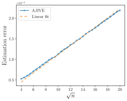
(a) Estimation error $\|\widehat{\bm{U}}\widehat{\bm{U}}^{\top}-\bm{U}^{\star}\bm{U}^{\star\top}\|$ vs $\sqrt{n}$. The parameter is chosen to be $K=100$ and $n$ ranges from 16 to 400.

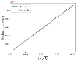
(b) Estimation error $\|\widehat{\bm{U}}\widehat{\bm{U}}^{\top}-\bm{U}^{\star}\bm{U}^{\star\top}\|$ vs $1/\sqrt{K}$. The parameter is chosen to be $n=20$ and $K$ ranges from 25 to 10000.

Figure 1: Estimation error when ${\theta}=1/2$. The parameters are chosen to be $d=20$, $r=2$, $\sigma=0.001$, and $\gamma=0.5$. The loading matrices use the random generation scheme. Each point is an average of 100 trials.

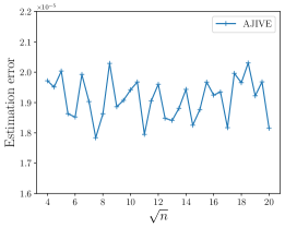
(a) Estimation error $\|\widehat{\bm{U}}\widehat{\bm{U}}^{\top}-\bm{U}^{\star}\bm{U}^{\star\top}\|$ vs $\sqrt{n}$.

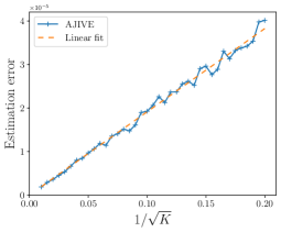
(b) Estimation error $\|\widehat{\bm{U}}\widehat{\bm{U}}^{\top}-\bm{U}^{\star}\bm{U}^{\star\top}\|$ vs $1/\sqrt{K}$.

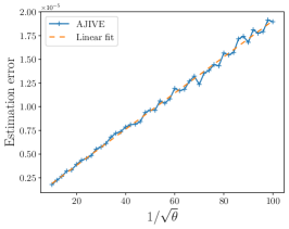
(c) Estimation error $\|\widehat{\bm{U}}\widehat{\bm{U}}^{\top}-\bm{U}^{\star}\bm{U}^{\star\top}\|$ vs $1/\sqrt{\theta}$.

Figure 2: Estimation error when $\widetilde{\theta}$ is small. The loading matrices use the random generation scheme. For all three subfigures, the parameters are $d=20$, $r=2$, $\sigma=10^{-6}$, and $\gamma=0.5$. In (a), $K=100$, $\theta=0.0001$ and $n$ ranges from 16 to 400. In (b), $n=20$, $\theta=0.0001$, and $K$ ranges from 25 to 10000. In (c), $n=20$, $K=100$, and $\theta$ ranges from $0.01$ to $0.0001$. Each point is an average of 100 trials.

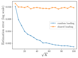
(a) Estimation error with Algorithm 1. The noise level is set to be $\sigma=0.01$.

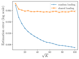
(b) Estimation error with Algorithm 2. The noise level is set to be $\sigma=0.1$.

Figure 3: Estimation error $\|\widehat{\bm{U}}\widehat{\bm{U}}^{\top}-\bm{U}^{\star}\bm{U}^{\star\top}\|$ vs $\sqrt{K}$ using random vs shared loading generation scheme. The parameters are chosen to be $n=d=20$, $r=2$, $\gamma=0.5$, and $K$ ranges from 25 to 10000. Each point is an average of 100 trials. The $y$-axis is in log scale.

Results.

Theorem 1 shows that when $r\asymp r_{\mathrm{avg}}\asymp 1$, AJIVE achieves estimation error

$$\left\|\widehat{\bm{U}}\widehat{\bm{U}}^{\top}-\bm{U}^{\star}\bm{U}^{\star\top}\right\|\lesssim\frac{\sigma}{\sigma_{\min}}\sqrt{\frac{n}{K}+\frac{r}{K\theta}}.$$ (14)

in the high-SNR regime. To highlight this error dependence, we set a small noise level $\sigma$.

• Figure 1 shows the performance of AJIVE when $\theta$ is large; we set $\theta=1/2$ in the experiment. In this case, we see from Figure 1 that the error scales linearly with $\sqrt{n}$ and $1/\sqrt{K}$.

• Figure 2 shows the performance of AJIVE when $\theta$ is small. In particular, Figures 2 and 2 fix a small $\theta=0.0001$. We clearly see that the error does not depend on the ambient dimension $n$, and decays linearly with $1/\sqrt{K}$. Moreover, Figure 2 fixes $n$ and $K$, and we see a clear linear dependence on $1/\sqrt{\theta}$.

All of these corroborate our theoretical prediction about AJIVE’s performance.

Another phenomenon we observe in Theorem 1 is that with a high signal-to-noise ratio, AJIVE can be inconsistent, i.e., the estimation error does not go to 0 as $K\rightarrow\infty$. Figure 3 demonstrates this stagnation under the shared loading scheme. Moreover, Figure 3 shows a similar persisting error with the oracle-aided Algorithm 2, supporting our oracle lower bound in Theorem 3. This observation underscores the challenge of estimating shared singular subspaces in this regime.

7 Discussion

In this paper, we analyzed the performance of the AJIVE algorithm for estimating the shared subspace from multiple data matrices. We provided new statistical guarantees on its performance, highlighting the power and potential limitations of multiple matrices in estimating the shared subspace. We also developed minimax lower bounds, demonstrating the optimality of AJIVE in the high-SNR regime.

Our analysis revealed that AJIVE achieves exact recovery in the noiseless case and exhibits first-order optimality in the high-SNR regime. Additionally, we confirmed the benefit of using multiple data matrices for estimation in this regime. However, we also observed that AJIVE suffers from a non-diminishing error in the low-SNR regime as the number of matrices increases.

To further investigate this non-diminishing error, we provided a performance lower bound for an oracle-aided spectral estimator. This analysis suggested that the non-diminishing error might be a fundamental limit of the problem, rather than an artifact of the AJIVE algorithm.

Our work provides a theoretical understanding of shared subspace estimation from multiple matrices. Future research directions include closing the gap between the upper and lower bounds in the low-SNR regime and exploring the potential of non-convex methods in this context.

Appendix A Additional experiments

In this section we show the results of some additional experiment that is omitted in the main text due to space constraint. We use the same experiment setting as Section 6.

We verify the first-order error dependency on $\sigma$ and $d$. In Figure 4, we can see that the estimation errors are about the same for different $d$. In Figure 4, we see that the estimation error scales linearly with the noise level $\sigma$.

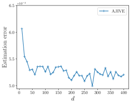
(a) Estimation error $\|\widehat{\bm{U}}\widehat{\bm{U}}^{\top}-\bm{U}^{\star}\bm{U}^{\star\top}\|$ vs $d$. The parameter is chosen to be $\sigma=10^{-3}$ and $d$ ranges from 10 to 400.

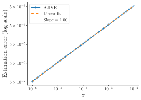
(b) Estimation error $\|\widehat{\bm{U}}\widehat{\bm{U}}^{\top}-\bm{U}^{\star}\bm{U}^{\star\top}\|$ vs $\sigma$. The parameter is chosen to be $d=20$ and $\sigma$ ranges from $10^{-6}$ to $10^{-3}$. Both $x$-axis and $y$-axis are in log scale.

Figure 4: Estimation error when $\widetilde{\theta}=1/2$. The parameters are chosen to be $n=20$, $r=2$, $K=100$, and $\gamma=0.5$. The loading matrices use the random generation scheme. Each point is an average of 100 trials.

Appendix B Expectation of monomials of the noise

In this section we collect some generic results about the expectation of monomials of $\bm{E}\in\mathbb{R}^{n_{1}\times n_{2}}$, which is a random matrix whose entries are i.i.d. Gaussian random variables with variance $\sigma^{2}$. These results will be helpful in proving Lemma 10. As any odd degree monomial of $\bm{E}$ is zero-mean, we focus on degree 2 and 4 monomials here. By linearity of expectation, we only need to compute those monomials in the form of $\bm{E}_{1}\bm{A}\bm{E}_{2}$ and $\bm{E}_{1}\bm{A}\bm{E}_{2}\bm{B}\bm{E}_{3}\bm{C}\bm{E}_{4}$, where $\bm{A},\bm{B},\bm{C}$ are generic matrices and $\bm{E}_{i}$ is either $\bm{E}$ or $\bm{E}^{\top}$. Note that the flip all the transpose of $\bm{E}$ is equivalent to computing the expectation as a monomial of $\bm{E}^{\top}$, which is itself a random matrix with i.i.d. Gaussian noise. Hence we omit those monomials that are inherently repetitive.

We start with degree-2 monomials $\bm{E}\bm{A}\bm{E}$ and $\bm{E}\bm{A}\bm{E}^{\top}$. In addition we compute $\mathbb{E}[\mathrm{Trace}(\bm{E}\bm{A})\bm{E}]$ which is useful later in the analysis for the degree-4 monomials. The proof is deferred to Section B.1.

Lemma 1.

Let $\bm{E}$ be a $n_{1}\times n_{2}$ matrix where each entry $E_{ij}$ is a zero-mean Gaussian random variable with variance $\sigma^{2}$. Let $\bm{A}$ be a matrix of appropriate dimension. Then

$$\mathbb{E}[\bm{E}\bm{A}\bm{E}] =\sigma^{2}\bm{A}^{\top};$$

$$\mathbb{E}[\bm{E}\bm{A}\bm{E}^{\top}] =\sigma^{2}\mathrm{Trace}(\bm{A})\bm{I};$$

$$\mathbb{E}[\mathrm{Trace}(\bm{E}\bm{A})\bm{E}] =\sigma^{2}\bm{A}^{\top}.$$

Similarly we have the following lemma for degree-4 monomials. The proof is deferred to Section B.2.

Lemma 2.

Let $\bm{E}$ be a $n_{1}\times n_{2}$ matrix where each entry $E_{ij}$ is a zero-mean Gaussian random variable with variance $\sigma^{2}$. Let $\bm{A},\bm{B},\bm{C}$ be matrices of appropriate dimension. Then

$$\mathbb{E}\left[\bm{E}\bm{A}\bm{E}^{\top}\bm{B}\bm{E}\bm{C}\bm{E}^{\top}\right] =\sigma^{4}\mathrm{Trace}(\bm{C})\mathrm{Trace}(\bm{A})\bm{B}+\sigma^{4}\mathrm{Trace}(\bm{A}\bm{C}^{\top})\bm{B}^{\top}+\sigma^{4}\mathrm{Trace}(\bm{B})\mathrm{Trace}(\bm{AC})\bm{I}$$ (15a)

$$\mathbb{E}\left[\bm{E}\bm{A}\bm{E}\bm{B}\bm{E}^{\top}\bm{C}\bm{E}^{\top}\right] =\sigma^{4}\bm{A}^{\top}\bm{B}\bm{C}^{\top}+\sigma^{4}\bm{C}\bm{B}\bm{A}+\sigma^{4}\mathrm{Trace}(\bm{B})\mathrm{Trace}(\bm{AC})\bm{I}$$ (15b)

$$\mathbb{E}\left[\bm{E}^{\top}\bm{A}\bm{E}\bm{B}\bm{E}\bm{C}\bm{E}^{\top}\right] =\sigma^{4}\mathrm{Trace}(\bm{C})\mathrm{Trace}(\bm{A})\bm{B}+\sigma^{4}\bm{C}\bm{B}\bm{A}+\sigma^{4}\bm{C}^{\top}\bm{B}\bm{A}^{\top}$$ (15c)

$$\mathbb{E}\left[\bm{E}^{\top}\bm{A}\bm{E}\bm{B}\bm{E}\bm{C}\bm{E}\right] =\sigma^{4}\mathrm{Trace}(\bm{A})\bm{B}\bm{C}^{\top}+\sigma^{4}\bm{C}\bm{A}^{\top}\bm{B}^{\top}+\sigma^{4}\mathrm{Trace}(\bm{A}\bm{B}^{\top}\bm{C})\bm{I}$$ (15d)

$$\mathbb{E}\left[\bm{E}\bm{A}\bm{E}^{\top}\bm{B}\bm{E}\bm{C}\bm{E}\right] =\sigma^{4}\mathrm{Trace}(\bm{A})\bm{B}\bm{C}^{\top}+\sigma^{4}\bm{B}^{\top}\bm{C}^{\top}\bm{A}+\sigma^{4}\mathrm{Trace}(\bm{B})\bm{C}^{\top}\bm{A}^{\top}$$ (15e)

$$\mathbb{E}\left[\bm{E}\bm{A}\bm{E}\bm{B}\bm{E}^{\top}\bm{C}\bm{E}\right] =\sigma^{4}\mathrm{Trace}(\bm{C})\bm{A}^{\top}\bm{B}+\sigma^{4}\bm{C}\bm{A}^{\top}\bm{B}^{\top}+\sigma^{4}\mathrm{Trace}(\bm{B})\bm{C}^{\top}\bm{A}^{\top}$$ (15f)

$$\mathbb{E}\left[\bm{E}\bm{A}\bm{E}\bm{B}\bm{E}\bm{C}\bm{E}^{\top}\right] =\sigma^{4}\mathrm{Trace}(\bm{C})\bm{A}^{\top}\bm{B}+\sigma^{4}\bm{B}^{\top}\bm{C}^{\top}\bm{A}+\sigma^{4}\mathrm{Trace}(\bm{A}\bm{B}^{\top}\bm{C})\bm{I}$$ (15g)

$$\mathbb{E}\left[\bm{E}\bm{A}\bm{E}\bm{B}\bm{E}\bm{C}\bm{E}\right] =\sigma^{4}\bm{A}^{\top}\bm{B}\bm{C}^{\top}+\sigma^{4}\mathrm{Trace}(\bm{A}\bm{C}^{\top})\bm{B}^{\top}+\sigma^{4}\bm{C}^{\top}\bm{B}\bm{A}^{\top}.$$ (15h)

B.1 Proof of Lemma 1

We prove the equations in Lemma 1 in order.

$\mathbb{E}[\bm{E}\bm{A}\bm{E}]$.

For each $(i,j)\in[n_{1}]\times[n_{2}]$,

$$\mathbb{E}[\bm{E}\bm{A}\bm{E}]_{ij}=\sum_{k,l}\mathbb{E}\bm{E}_{ik}A_{kl}\bm{E}_{lj}=\mathbb{E}\bm{E}_{ij}A_{ji}\bm{E}_{ij}=\sigma^{2}A_{ji},$$

where the second equality holds since $\mathbb{E}\bm{E}_{ik}A_{kl}\bm{E}_{lj}=0$ if $i\neq l$ or $k\neq j$. Thus

$$\mathbb{E}[\bm{E}\bm{A}\bm{E}]=\sigma^{2}\bm{A}^{\top}.$$

$\mathbb{E}[\bm{E}\bm{A}\bm{E}^{\top}]$.

For each $(i,j)\in[n_{1}]\times[n_{2}]$, if $i\neq j$,

$$\mathbb{E}[\bm{E}\bm{A}\bm{E}^{\top}]_{ij}=\sum_{k,l}\mathbb{E}\bm{E}_{ik}A_{kl}\bm{E}_{jl}=0$$

If $i=j$,

$$\mathbb{E}[\bm{E}\bm{A}\bm{E}^{\top}]_{ii} =\sum_{k,l}\mathbb{E}\bm{E}_{ik}A_{kl}\bm{E}_{il}=\sum_{k}\mathbb{E}\bm{E}_{ik}A_{kk}\bm{E}_{ik}=\sigma^{2}\mathrm{Trace}(\bm{A}).$$

Then $\mathbb{E}[\bm{E}\bm{A}\bm{E}^{\top}]=\sigma^{2}\mathrm{Trace}(\bm{A})\bm{I}$.

$\mathbb{E}[\mathrm{Trace}(\bm{E}\bm{A})\bm{E}]$.

For each $(i,j)$,

$$\mathbb{E}[\mathrm{Trace}(\bm{E}\bm{A})\bm{E}]_{ij}=\mathbb{E}[\mathrm{Trace}(\bm{E}\bm{A})E_{ij}]=\mathbb{E}\left(\sum_{k}\sum_{l}E_{kl}A_{lk}\right)E_{ij}=\mathbb{E}E_{ij}A_{ji}E_{ij}=\sigma^{2}A_{ji}.$$

Then

$$\mathbb{E}[\mathrm{Trace}(\bm{E}\bm{A})\bm{E}]=\sigma^{2}\bm{A}^{\top}.$$

B.2 Proof of Lemma 2

This proof is inspired by results in [NW87], which gives a formula for $\mathbb{E}\left[\bm{E}\bm{A}\bm{E}^{\top}\bm{B}\bm{E}\bm{C}\bm{E}^{\top}\right]$. It is proved using the following argument:

Expand $\mathbb{E}\left[\bm{E}\bm{A}\bm{E}^{\top}\bm{B}\bm{E}\bm{C}\bm{E}^{\top}\right]$ as a polynomial of real valued random variables $E_{ij}$. Consider a degree-four monomial $abcE_{i_{1}j_{1}}E_{i_{2}j_{2}}E_{i_{3}j_{3}}E_{i_{4}j_{4}}$, where $a,b,c$ are some scalars. by Isserlis’s theorem ([Iss18]), we have that

$$abc\mathbb{E}E_{i_{1}j_{1}}E_{i_{2}j_{2}}E_{i_{3}j_{3}}E_{i_{4}j_{4}} =abc\mathbb{E}\left[E_{i_{1}j_{1}}E_{i_{2}j_{2}}\right]\mathbb{E}\left[E_{i_{3}j_{3}}E_{i_{4}j_{4}}\right]$$

$$\quad+abc\mathbb{E}\left[E_{i_{1}j_{1}}E_{i_{3}j_{3}}\right]\mathbb{E}\left[E_{i_{2}j_{2}}E_{i_{4}j_{4}}\right]$$

$$\quad+abc\mathbb{E}\left[E_{i_{1}j_{1}}E_{i_{4}j_{4}}\right]\mathbb{E}\left[E_{i_{2}j_{2}}E_{i_{3}j_{3}}\right].$$

Now we putting this back to the polynomial of $\mathbb{E}\left[\bm{E}\bm{A}\bm{E}^{\top}\bm{B}\bm{E}\bm{C}\bm{E}^{\top}\right]$. To help with the notation, we label the four occurrences of $\bm{E}$ as $\bm{E}_{1},\bm{E}_{2},\bm{E}_{3},\bm{E}_{4}$ without altering their meaning. We also label the expectation sign $\mathbb{E}_{ij}$ to indicate that the expectation is taken for $\bm{E}_{i}$ and $\bm{E}_{j}$, treating all other matrices as constants. Combining all terms, we have that

$$\mathbb{E}\left[\bm{E}_{1}\bm{A}\bm{E}_{2}^{\top}\bm{B}\bm{E}_{3}\bm{C}\bm{E}_{4}^{\top}\right] =\mathbb{E}_{12}\left[\bm{E}_{1}\bm{A}\bm{E}_{2}^{\top}\bm{B}\mathbb{E}_{34}\left[\bm{E}_{3}\bm{C}\bm{E}_{4}^{\top}\right]\right]$$

$$\quad+\mathbb{E}_{13}\left[\bm{E}_{1}\bm{A}\mathbb{E}_{24}\left[\bm{E}_{2}^{\top}\bm{B}\bm{E}_{3}\bm{C}\bm{E}_{4}^{\top}\right]\right]$$

$$\quad+\mathbb{E}_{14}\left[\bm{E}_{1}\bm{A}\mathbb{E}_{23}\left[\bm{E}_{2}^{\top}\bm{B}\bm{E}_{3}\right]\bm{C}\bm{E}_{4}^{\top}\right].$$

Using the same idea, we can get (15a) to (15h) by substituting some of the $\bm{E}_{i}$’s with their transpose and simplifying the equation with Lemma 1. We include all the detailed steps in the rest of this section.

Proof of (15a).

$$\mathbb{E}\left[\bm{E}\bm{A}\bm{E}^{\top}\bm{B}\bm{E}\bm{C}\bm{E}^{\top}\right] =\mathbb{E}\left[\bm{E}_{1}\bm{A}\bm{E}_{2}^{\top}\bm{B}\mathbb{E}_{34}[\bm{E}_{3}\bm{C}\bm{E}_{4}^{\top}]\right]+\mathbb{E}\left[\bm{E}\bm{A}\mathbb{E}_{24}[\bm{E}_{2}^{\top}\bm{B}\bm{E}_{3}\bm{C}\bm{E}_{4}^{\top}]\right]$$

$$\quad+\mathbb{E}\left[\bm{E}_{1}\bm{A}\mathbb{E}_{23}[\bm{E}_{2}^{\top}\bm{B}\bm{E}_{3}]\bm{C}\bm{E}_{4}^{\top}\right]$$

$$=\sigma^{2}\mathrm{Trace}(\bm{C})\mathbb{E}\left[\bm{E}_{1}\bm{A}\bm{E}_{2}^{\top}\bm{B}\right]+\sigma^{2}\mathbb{E}\left[\bm{E}\bm{A}\bm{C}^{\top}\bm{E}_{3}^{\top}\bm{B}^{\top}\right]$$

$$\quad+\sigma^{2}\mathrm{Trace}(\bm{B})\mathbb{E}\left[\bm{E}_{1}\bm{A}\bm{C}\bm{E}_{4}^{\top}\right]$$

$$=\sigma^{4}\mathrm{Trace}(\bm{C})\mathrm{Trace}(\bm{A})\bm{B}+\sigma^{4}\mathrm{Trace}(\bm{A}\bm{C}^{\top})\bm{B}^{\top}+\sigma^{4}\mathrm{Trace}(\bm{B})\mathrm{Trace}(\bm{AC})\bm{I}.$$

Proof of (15b).

$$\mathbb{E}\left[\bm{E}\bm{A}\bm{E}\bm{B}\bm{E}^{\top}\bm{C}\bm{E}^{\top}\right] =\mathbb{E}\left[\bm{E}_{1}\bm{A}\bm{E}_{2}\bm{B}\mathbb{E}_{34}[\bm{E}_{3}^{\top}\bm{C}\bm{E}_{4}^{\top}]\right]+\mathbb{E}\left[\bm{E}\bm{A}\mathbb{E}_{24}[\bm{E}_{2}\bm{B}\bm{E}_{3}^{\top}\bm{C}\bm{E}_{4}^{\top}]\right]$$

$$\quad+\mathbb{E}\left[\bm{E}_{1}\bm{A}\mathbb{E}_{23}[\bm{E}_{2}\bm{B}\bm{E}_{3}^{\top}]\bm{C}\bm{E}_{4}^{\top}\right]$$

$$=\sigma^{2}\mathbb{E}\left[\bm{E}_{1}\bm{A}\bm{E}_{2}\bm{B}\bm{C}^{\top}\right]+\sigma^{2}\mathbb{E}\left[\bm{E}\bm{A}\mathrm{Trace}(\bm{B}\bm{E}_{3}^{\top}\bm{C})\right]$$

$$\quad+\sigma^{2}\mathrm{Trace}(\bm{B})\mathbb{E}\left[\bm{E}_{1}\bm{A}\bm{C}\bm{E}_{4}^{\top}\right]$$

$$=\sigma^{4}\bm{A}^{\top}\bm{B}\bm{C}^{\top}+\sigma^{4}\bm{C}\bm{B}\bm{A}+\sigma^{4}\mathrm{Trace}(\bm{B})\mathrm{Trace}(\bm{AC})\bm{I}.$$

Proof of (15c).

$$\mathbb{E}\left[\bm{E}^{\top}\bm{A}\bm{E}\bm{B}\bm{E}\bm{C}\bm{E}^{\top}\right] =\mathbb{E}\left[\bm{E}_{1}^{\top}\bm{A}\bm{E}_{2}\bm{B}\mathbb{E}_{34}[\bm{E}\bm{C}\bm{E}^{\top}]\right]+\mathbb{E}\left[\bm{E}_{1}^{\top}\bm{A}\mathbb{E}_{24}[\bm{E}\bm{B}\bm{E}\bm{C}\bm{E}^{\top}]\right]$$

$$\quad+\mathbb{E}\left[\bm{E}_{1}^{\top}\bm{A}\mathbb{E}_{23}[\bm{E}\bm{B}\bm{E}]\bm{C}\bm{E}_{4}^{\top}\right]$$

$$=\sigma^{2}\mathrm{Trace}(\bm{C})\mathbb{E}\left[\bm{E}_{1}^{\top}\bm{A}\bm{E}_{2}\bm{B}\right]+\sigma^{2}\mathbb{E}\left[\bm{E}_{1}^{\top}\bm{A}\mathrm{Trace}(\bm{B}\bm{E}_{3}\bm{C})\right]$$

$$\quad+\sigma^{2}\mathbb{E}\left[\bm{E}_{1}^{\top}\bm{A}\bm{B}^{\top}\bm{C}\bm{E}_{4}^{\top}\right]$$

$$=\sigma^{4}\mathrm{Trace}(\bm{C})\mathrm{Trace}(\bm{A})\bm{B}+\sigma^{4}\bm{C}\bm{B}\bm{A}+\sigma^{4}\bm{C}^{\top}\bm{B}\bm{A}^{\top}.$$

Proof of (15d).

$$\mathbb{E}\left[\bm{E}^{\top}\bm{A}\bm{E}\bm{B}\bm{E}\bm{C}\bm{E}\right] =\mathbb{E}\left[\bm{E}_{1}^{\top}\bm{A}\bm{E}_{2}\bm{B}\mathbb{E}_{34}[\bm{E}_{3}\bm{C}\bm{E}_{4}]\right]+\mathbb{E}\left[\bm{E}_{1}^{\top}\bm{A}\mathbb{E}_{24}[\bm{E}_{2}\bm{B}\bm{E}_{3}\bm{C}\bm{E}_{4}]\right]$$

$$\quad+\mathbb{E}\left[\bm{E}_{1}^{\top}\bm{A}\mathbb{E}_{23}[\bm{E}_{2}\bm{B}\bm{E}_{3}]\bm{C}\bm{E}_{4}\right]$$

$$=\sigma^{2}\mathbb{E}\left[\bm{E}_{1}^{\top}\bm{A}\bm{E}_{2}\bm{B}\bm{C}^{\top}\right]+\sigma^{2}\mathbb{E}\left[\bm{E}_{1}^{\top}\bm{A}\bm{C}^{\top}\bm{E}_{3}^{\top}\bm{B}^{\top}\right]$$

$$\quad+\sigma^{2}\mathbb{E}\left[\bm{E}_{1}^{\top}\bm{A}\bm{B}^{\top}\bm{C}\bm{E}_{4}\right]$$

$$=\sigma^{4}\mathrm{Trace}(\bm{A})\bm{B}\bm{C}^{\top}+\sigma^{4}\bm{C}\bm{A}^{\top}\bm{B}^{\top}+\sigma^{4}\mathrm{Trace}(\bm{A}\bm{B}^{\top}\bm{C})\bm{I}.$$

Proof of (15e).

$$\mathbb{E}\left[\bm{E}\bm{A}\bm{E}^{\top}\bm{B}\bm{E}\bm{C}\bm{E}\right] =\mathbb{E}\left[\bm{E}\bm{A}\bm{E}^{\top}\bm{B}\mathbb{E}_{34}[\bm{E}\bm{C}\bm{E}]\right]+\mathbb{E}\left[\bm{E}_{1}^{\top}\bm{A}\mathbb{E}_{24}[\bm{E}_{2}\bm{B}\bm{E}_{3}^{\top}\bm{C}\bm{E}_{4}^{\top}]\right]$$

$$\quad+\mathbb{E}\left[\bm{E}_{1}\bm{A}\mathbb{E}_{23}[\bm{E}_{2}^{\top}\bm{B}\bm{E}_{3}]\bm{C}\bm{E}_{4}\right]$$

$$=\sigma^{2}\mathbb{E}\left[\bm{E}_{1}\bm{A}\bm{E}_{2}^{\top}\bm{B}\bm{C}^{\top}\right]+\sigma^{2}\mathbb{E}\left[\bm{E}_{1}\bm{A}\mathrm{Trace}(\bm{B}\bm{E}_{3}^{\top}\bm{C})\right]$$

$$\quad+\sigma^{2}\mathrm{Trace}(\bm{B})\mathbb{E}\left[\bm{E}_{1}\bm{A}\bm{C}\bm{E}_{4}\right]$$

$$=\sigma^{4}\mathrm{Trace}(\bm{A})\bm{B}\bm{C}^{\top}+\sigma^{4}\bm{B}^{\top}\bm{C}^{\top}\bm{A}+\sigma^{4}\mathrm{Trace}(\bm{B})\bm{C}^{\top}\bm{A}^{\top}.$$

Proof of (15f).

$$\mathbb{E}\left[\bm{E}\bm{A}\bm{E}\bm{B}\bm{E}^{\top}\bm{C}\bm{E}\right] =\mathbb{E}\left[\bm{E}_{1}\bm{A}\bm{E}_{2}\bm{B}\mathbb{E}_{34}[\bm{E}_{3}^{\top}\bm{C}\bm{E}_{4}]\right]+\mathbb{E}\left[\bm{E}_{1}\bm{A}\mathbb{E}_{24}[\bm{E}_{2}\bm{B}\bm{E}_{3}^{\top}\bm{C}\bm{E}_{4}]\right]$$

$$\quad+\mathbb{E}\left[\bm{E}_{1}\bm{A}\mathbb{E}_{23}[\bm{E}_{2}\bm{B}\bm{E}_{3}^{\top}]\bm{C}\bm{E}_{4}\right]$$

$$=\sigma^{2}\mathrm{Trace}(\bm{C})\mathbb{E}\left[\bm{E}_{1}\bm{A}\bm{E}_{2}\bm{B}\right]+\sigma^{2}\mathbb{E}\left[\bm{E}_{1}\bm{A}\bm{C}^{\top}\bm{E}_{3}\bm{B}^{\top}\right]$$

$$\quad+\sigma^{2}\mathrm{Trace}(\bm{B})\mathbb{E}\left[\bm{E}_{1}\bm{A}\bm{C}\bm{E}_{4}\right]$$

$$=\sigma^{4}\mathrm{Trace}(\bm{C})\bm{A}^{\top}\bm{B}+\sigma^{4}\bm{C}\bm{A}^{\top}\bm{B}^{\top}+\sigma^{4}\mathrm{Trace}(\bm{B})\bm{C}^{\top}\bm{A}^{\top}.$$

Proof of (15g).

$$\mathbb{E}\left[\bm{E}\bm{A}\bm{E}\bm{B}\bm{E}\bm{C}\bm{E}^{\top}\right] =\mathbb{E}\left[\bm{E}_{1}\bm{A}\bm{E}_{2}\bm{B}\mathbb{E}_{34}[\bm{E}_{3}\bm{C}\bm{E}_{4}^{\top}]\right]+\mathbb{E}\left[\bm{E}_{1}\bm{A}\mathbb{E}_{24}[\bm{E}_{2}\bm{B}\bm{E}_{3}\bm{C}\bm{E}_{4}^{\top}]\right]$$

$$\quad+\mathbb{E}\left[\bm{E}_{1}\bm{A}\mathbb{E}_{23}[\bm{E}_{2}\bm{B}\bm{E}_{3}]\bm{C}\bm{E}_{4}^{\top}\right]$$

$$=\sigma^{2}\mathrm{Trace}(\bm{C})\mathbb{E}\left[\bm{E}_{1}\bm{A}\bm{E}_{2}\bm{B}\right]+\sigma^{2}\mathbb{E}\left[\bm{E}_{1}\bm{A}\mathrm{Trace}(\bm{B}\bm{E}_{3}\bm{C})\right]$$

$$\quad+\sigma^{2}\mathbb{E}\left[\bm{E}_{1}\bm{A}\bm{B}^{\top}\bm{C}\bm{E}_{4}^{\top}\right]$$

$$=\sigma^{4}\mathrm{Trace}(\bm{C})\bm{A}^{\top}\bm{B}+\sigma^{4}\bm{B}^{\top}\bm{C}^{\top}\bm{A}+\sigma^{4}\mathrm{Trace}(\bm{A}\bm{B}^{\top}\bm{C})\bm{I}.$$

Proof of (15h).

$$\mathbb{E}\left[\bm{E}\bm{A}\bm{E}\bm{B}\bm{E}\bm{C}\bm{E}\right] =\mathbb{E}\left[\bm{E}_{1}\bm{A}\bm{E}_{2}\bm{B}\mathbb{E}_{34}[\bm{E}_{3}\bm{C}\bm{E}_{4}]\right]+\mathbb{E}\left[\bm{E}\bm{A}\mathbb{E}_{24}[\bm{E}_{2}\bm{B}\bm{E}_{3}\bm{C}\bm{E}_{4}]\right]$$

$$\quad+\mathbb{E}\left[\bm{E}_{1}\bm{A}\mathbb{E}_{23}[\bm{E}_{2}\bm{B}\bm{E}_{3}]\bm{C}\bm{E}_{4}\right]$$

$$=\sigma^{2}\mathbb{E}\left[\bm{E}_{1}\bm{A}\bm{E}_{2}\bm{B}\bm{C}^{\top}\right]+\sigma^{2}\mathbb{E}\left[\bm{E}\bm{A}\bm{C}^{\top}\bm{E}_{3}^{\top}\bm{B}^{\top}\right]$$

$$\quad+\sigma^{2}\mathbb{E}\left[\bm{E}_{1}\bm{A}\bm{B}^{\top}\bm{C}\bm{E}_{4}\right]$$

$$=\sigma^{4}\bm{A}^{\top}\bm{B}\bm{C}^{\top}+\sigma^{4}\mathrm{Trace}(\bm{A}\bm{C}^{\top})\bm{B}^{\top}+\sigma^{4}\bm{C}^{\top}\bm{B}\bm{A}^{\top}.$$

Appendix C Proof of Theorem 1

We prove a more detailed theorem here.

Theorem 4.

Instate the assumptions of Theorem 1, we have that with probability at least $1-O(KN^{-10})$,

$$\left\|\widehat{\bm{U}}\widehat{\bm{U}}^{\top}-\bm{U}^{\star}\bm{U}^{\star\top}\right\|\leq C_{1}\left[\frac{\sigma}{\sigma_{\min}}\left(\sqrt{\frac{n}{K}+\frac{r+r_{\mathrm{avg}}}{K\theta}+\frac{r\cdot r_{\mathrm{avg}}}{K\theta}\wedge\frac{r}{K^{2}\theta^{2}}}\right)\log^{5/2}N\right.$$

$$\qquad+\frac{\sigma^{2}}{\sigma_{\min}^{2}}\sqrt{\frac{nd}{K}+\frac{d(r+r_{\mathrm{avg}})}{K\theta}+\left(nd+n^{2}\right)\left(\frac{3r_{\mathrm{avg}}}{K\theta}\wedge\frac{1}{K^{2}\theta^{2}}\right)}\log N.$$

$$\qquad+\frac{1}{\theta}\left(\frac{\kappa^{2}\sigma^{2}n}{\sigma_{\min}^{2}}+\frac{\sigma^{4}(nd+n^{2})}{\sigma_{\min}^{4}}\right)$$

$$\qquad+\frac{\sigma^{2}n}{\sigma_{\min}^{2}}\left(\frac{\log N}{K\theta^{2}}+\frac{\log^{2}N}{K^{2}\theta^{2}}\right)$$

$$\qquad\left.+\frac{\sigma^{4}}{\sigma_{\min}^{4}}\left(\frac{nd\log N}{K\theta^{2}}+\frac{(nd+n^{2})\log^{2}N}{K^{2}\theta^{2}}\right)\right]$$

for some constant $C_{1}>0$.

It is easy to see that the following theorem can be simplified to Theorem 1 by using Assumption (6) and taking the worst log dependency. It is worth noting that when $d\gg n$, this complete theorem offers a better dependency on the dimension for second-order term that does not scale with $K$. Ignoring the log factors, the dependency of the upper bound of on $\sigma^{2}/\sigma_{\min}^{2}$ is

$$\frac{1}{\theta(K\theta\wedge 1)}\cdot\frac{\kappa^{2}\sigma^{2}n}{\sigma_{\min}^{2}}$$

in Theorem 4 and

$$\frac{1}{\theta(K\theta\wedge 1)}\cdot\frac{\kappa^{2}\sigma^{2}(\sqrt{nd}+n)}{\sigma_{\min}^{2}}$$

in the simplified Theorem 1.

We now begin the proof for Theorem 4. The key of the proof of this theorem is the use of a first-order approximation result in [Xia21] on SVD. We first establish a first-order approximation of $\widetilde{\bm{U}}_{k}\widetilde{\bm{U}}_{k}^{\top}$, and then a first-order approximation of $\widehat{\bm{U}}\widehat{\bm{U}}^{\top}$. This then allow us to control the estimation error $\|\bm{U}^{\star}\bm{U}^{\star\top}-\widehat{\bm{U}}\widehat{\bm{U}}^{\top}\|$ by controlling the first-order terms, resulting in a first-order optimal error bound.

We start with $\widetilde{\bm{U}}_{k}\widetilde{\bm{U}}_{k}^{\top}$. For any $k\in[K]$, let the top-$(r+r_{k})$ SVD of $\bm{A}_{k}^{\star}$ be $\widetilde{\bm{U}}_{k}^{\star}\widetilde{\bm{\Sigma}}_{k}^{\star}\widetilde{\bm{V}}_{k}^{\star\top}$. Since $\mathrm{rank}(\bm{A}_{k}^{\star})=r+r_{k}$, $\mathrm{col}(\bm{A}_{k}^{\star})=\mathrm{col}(\widetilde{\bm{U}}_{k}^{\star})=\mathrm{col}(\bm{U}^{\star})+\mathrm{col}(\bm{U}_{k}^{\star})$ and we can write it as

$$\widetilde{\bm{U}}_{k}^{\star}\widetilde{\bm{U}}_{k}^{\star\top}=\bm{U}^{\star}\bm{U}^{\star\top}+\bm{U}_{k}^{\star}\bm{U}_{k}^{\star\top}.$$

We also define the matrices $\bm{P}_{k}^{\perp}$ and $\bm{P}_{k}^{-1}$ as $\bm{P}_{k}^{\perp}\coloneqq\bm{I}_{n}-\widetilde{\bm{U}}_{k}^{\star}\widetilde{\bm{U}}_{k}^{\star\top}$ and $\bm{P}_{k}^{-1}\coloneqq\widetilde{\bm{U}}_{k}^{\star}\widetilde{\bm{\Sigma}}_{k}^{\star-2}\widetilde{\bm{U}}_{k}^{\star\top}$. We have the following first order approximation of $\widetilde{\bm{U}}_{k}\widetilde{\bm{U}}_{k}^{\top}$.

Lemma 3.

Instate the assumptions of Theorem 1. Then with probability at least $1-O(KN^{-11})$, for every $k\in[K]$,

$$\widetilde{\bm{U}}_{k}\widetilde{\bm{U}}_{k}^{\top}=\widetilde{\bm{U}}_{k}^{\star}\widetilde{\bm{U}}_{k}^{\star\top}+\bm{B}_{k}+\bm{B}_{k}^{\top}+\bm{R}_{k},$$

where

$$\bm{B}_{k}\coloneqq\bm{P}_{k}^{\perp}\bm{E}_{k}\widetilde{\bm{V}}_{k}^{\star}\widetilde{\bm{\Sigma}}_{k}^{\star-1}\widetilde{\bm{U}}_{k}^{\star\top}+\bm{P}_{k}^{\perp}\left(\bm{E}_{k}\bm{E}_{k}^{\top}-d_{k}\sigma^{2}\bm{I}_{n}\right)\bm{P}_{k}^{-1}$$

and $\bm{R}_{k}$ is some $n\times n$ matrix such that

$$\|\bm{R}_{k}\|\leq C_{1}\left(\frac{\kappa^{2}\sigma^{2}n}{\sigma_{\min}^{2}}+\frac{\sigma^{4}(nd_{k}+n^{2})}{\sigma_{\min}^{4}}\right)$$

for some constant $C_{1}>0$.

Moreover, the following lemma controls the overall size of the first-order perturbation terms.

Lemma 4.

Instate the assumptions of Theorem 1. We have that with probability $1-O(KN^{-10})$,

$$\left\|\frac{1}{K}\sum_{k=1}^{K}\bm{B}_{k}\right\| \leq C_{2}\cdot\frac{\sigma\sqrt{n}}{\sigma_{\min}}\left(\sqrt{\frac{\log N}{K}}+\frac{\log N}{K}\right)$$

$$\qquad+C_{3}\cdot\frac{\sigma^{2}}{\sigma_{\min}^{2}}\left(\sqrt{\frac{nd\log N}{K}}+\frac{\left(\sqrt{nd}+n\right)\log N}{K}\right)$$

for some constants $C_{2},C_{3}>0$.

Lemma 3 and 4 show that

$$\|\bm{\Delta}\| \leq C_{2}\cdot\frac{\sigma\sqrt{n}}{\sigma_{\min}}\left(\sqrt{\frac{\log N}{K}}+\frac{\log N}{K}\right)$$ (16)

$$\qquad+C_{3}\cdot\frac{\sigma^{2}}{\sigma_{\min}^{2}}\left(\sqrt{\frac{nd\log N}{K}}+\frac{\left(\sqrt{nd}+n\right)\log N}{K}\right)$$

$$\qquad+C_{1}\left(\frac{\kappa^{2}\sigma^{2}n}{\sigma_{\min}^{2}}+\frac{\sigma^{4}(nd+n^{2})}{\sigma_{\min}^{4}}\right)\leq\theta/8.$$

Here the last inequality comes from Assumption (6).

We now introduce the notations necessary for the first-order approximation of $\widehat{\bm{U}}\widehat{\bm{U}}^{\top}$. Let

$$\bm{\Delta} \coloneqq\frac{1}{K}\sum_{k=1}^{K}\left(\bm{B}_{k}+\bm{B}_{k}^{\top}+\bm{R}_{k}\right);$$ (17a)

$$\bm{P} \coloneqq\bm{I}_{n}-\frac{1}{K}\sum_{k=1}^{K}\widetilde{\bm{U}}_{k}^{\star}\widetilde{\bm{U}}_{k}^{\star\top}=\bm{I}_{n}-\bm{U}^{\star}\bm{U}^{\star\top}-\frac{1}{K}\sum_{k=1}^{K}\bm{U}_{k}^{\star}\bm{U}_{k}^{\star\top}.$$ (17b)

As $\|K^{-1}\sum_{k=1}^{K}\bm{U}_{k}^{\star}\bm{U}_{k}^{\star\top}\|<1$, $\mathrm{rank}(\bm{P})=n-r$. Let its eigen-decomposition be

$$\bm{P}=\sum_{i=1}^{n-r}\mu_{i}\bm{x}_{i}\bm{x}_{i}^{\top},$$ (18)

where $\mu_{i}\in\mathbb{R}$ and $\{\bm{x}_{i}\}_{i\in[n-r]}$ are mutually orthogonal unit vectors. We can then define

$$\bm{P}^{-1} \coloneqq\sum_{i=1}^{n-r}\mu_{i}^{-1}\bm{x}_{i}\bm{x}_{i}^{\top};$$

$$\bm{P}^{\perp} \coloneqq\bm{U}^{\star}\bm{U}^{\star\top}.$$

We are now ready to state the following lemma, which gives a first-order approximation of $\widehat{\bm{U}}\widehat{\bm{U}}^{\top}$.

Lemma 5.

Instate the assumptions of Theorem 1. Then with probability at least $1-O(KN^{-10})$,

$$\widehat{\bm{U}}\widehat{\bm{U}}^{\top}=\bm{U}^{\star}\bm{U}^{\star\top}+\bm{P}^{-1}\bm{\Delta}\bm{P}^{\perp}+\bm{P}^{\perp}\bm{\Delta}\bm{P}^{-1}+\bm{R}$$ (19)

where $\bm{R}$ is some $n\times n$ matrix such that

$$\|\bm{R}\|\leq\frac{32\|\bm{\Delta}\|^{2}}{\theta{}^{2}}.$$ (20)

Furthermore, the following lemma controls the size of first-order perturbation.

Lemma 6.

Instate the assumptions of Theorem 1. We have that with probability at least $1-O(KN^{-10})$,

$$\left\|\bm{P}^{-1}\bm{\Delta}\bm{P}^{\perp}\right\| \leq C_{4}\frac{\sigma}{\sigma_{\min}}\left(\sqrt{\frac{n}{K}+\frac{r+r_{\mathrm{avg}}}{K\theta}+\frac{r\cdot r_{\mathrm{avg}}}{K\theta}\wedge\frac{r}{K^{2}\theta^{2}}}\right)\log^{5/2}N$$ (21)

$$\qquad+C_{5}\frac{\sigma^{2}}{\sigma_{\min}^{2}}\sqrt{\frac{nd}{K}+\frac{d(r+r_{\mathrm{avg}})}{K\theta}+\left(nd+n^{2}\right)\left(\frac{3r_{\mathrm{avg}}}{K\theta}\wedge\frac{1}{K^{2}\theta^{2}}\right)}\log N.$$

$$\qquad+\frac{C_{6}}{\theta}\left(\frac{\kappa^{2}\sigma^{2}n}{\sigma_{\min}^{2}}+\frac{\sigma^{4}(nd+n^{2})}{\sigma_{\min}^{4}}\right).$$

for some constants $C_{4},C_{5},C_{6}>0$.

We are now ready to bound the estimation error $\|\widehat{\bm{U}}\widehat{\bm{U}}^{\top}-\bm{U}^{\star}\bm{U}^{\star\top}\|$. Combining (16), (19), (20), and (21), we reach the conclusion that

$$\left\|\widehat{\bm{U}}\widehat{\bm{U}}^{\top}-\bm{U}^{\star}\bm{U}^{\star\top}\right\| \leq 2\left\|\bm{P}^{-1}\bm{\Delta}\bm{P}^{\perp}\right\|+\|\bm{R}\|$$

$$\leq 2C_{7}\left[\frac{\sigma}{\sigma_{\min}}\left(\sqrt{\frac{n}{K}+\frac{r+r_{\mathrm{avg}}}{K\theta}+\frac{r\cdot r_{\mathrm{avg}}}{K\theta}\wedge\frac{r}{K^{2}\theta^{2}}}\right)\log^{5/2}N\right.$$

$$\qquad+\frac{\sigma^{2}}{\sigma_{\min}^{2}}\sqrt{\frac{nd}{K}+\frac{d(r+r_{\mathrm{avg}})}{K\theta}+\left(nd+n^{2}\right)\left(\frac{3r_{\mathrm{avg}}}{K\theta}\wedge\frac{1}{K^{2}\theta^{2}}\right)}\log N.$$

$$\qquad+\frac{1}{\theta}\left(\frac{\kappa^{2}\sigma^{2}n}{\sigma_{\min}^{2}}+\frac{\sigma^{4}(nd+n^{2})}{\sigma_{\min}^{4}}\right)$$

$$\qquad+\frac{\sigma^{2}n}{\sigma_{\min}^{2}}\left(\frac{\log N}{K\theta^{2}}+\frac{\log^{2}N}{K^{2}\theta^{2}}\right)$$

$$\qquad\left.+\frac{\sigma^{4}}{\sigma_{\min}^{4}}\left(\frac{nd\log N}{K\theta^{2}}+\frac{\left(\sqrt{nd}+n\right)^{2}\log^{2}N}{K^{2}\theta^{2}}\right)\right].$$

C.1 Proof of Lemma 3

Consider the Gram matrix $\bm{A}_{k}\bm{A}_{k}^{\top}$. Using the definition of SVD of $\bm{A}^{\star}$, we have that

$$\bm{A}_{k}\bm{A}_{k}^{\top} =\left(\widetilde{\bm{U}}_{k}^{\star}\widetilde{\bm{\Sigma}}_{k}^{\star}\widetilde{\bm{V}}_{k}^{\star\top}+\bm{E}_{k}\right)\left(\widetilde{\bm{U}}_{k}^{\star}\widetilde{\bm{\Sigma}}_{k}^{\star}\widetilde{\bm{V}}_{k}^{\star\top}+\bm{E}_{k}\right)^{\top}$$

$$=\widetilde{\bm{U}}_{k}^{\star}\widetilde{\bm{\Sigma}}_{k}^{\star 2}\widetilde{\bm{U}}_{k}^{\star\top}+\bm{E}_{k}\widetilde{\bm{V}}_{k}^{\star}\widetilde{\bm{\Sigma}}_{k}^{\star}\widetilde{\bm{U}}_{k}^{\star\top}+\widetilde{\bm{U}}_{k}^{\star}\widetilde{\bm{\Sigma}}_{k}^{\star}\widetilde{\bm{V}}_{k}^{\star\top}\bm{E}_{k}^{\top}+\bm{E}_{k}\bm{E}_{k}^{\top}.$$

Recall that the columns of $\widetilde{\bm{U}}_{k}$ are the top-$(r+r_{k})$ left singular vectors of $\bm{A}_{k}$. Then equivalently, these columns are also the top-$(r+r_{k})$ eigenvectors of $\bm{A}_{k}\bm{A}_{k}^{\top}-d_{k}\sigma^{2}\bm{I}_{n}$.

We will now first present an first-order approximation $\widetilde{\bm{U}}_{k}\widetilde{\bm{U}}_{k}^{\top}$ based on the eigen-decomposition. Treat $\widetilde{\bm{U}}_{k}^{\star}\widetilde{\bm{\Sigma}}_{k}^{\star 2}\widetilde{\bm{U}}_{k}^{\star\top}$ as the ground truth and

$$\bm{\Delta}_{k}\coloneqq\bm{E}_{k}\widetilde{\bm{V}}_{k}^{\star}\widetilde{\bm{\Sigma}}_{k}^{\star}\widetilde{\bm{U}}_{k}^{\star\top}+\widetilde{\bm{U}}_{k}^{\star}\widetilde{\bm{\Sigma}}_{k}^{\star}\widetilde{\bm{V}}_{k}^{\star\top}\bm{E}_{k}^{\top}+\bm{E}_{k}\bm{E}_{k}^{\top}-d_{k}\sigma^{2}\bm{I}_{n}$$

as the perturbation.

We first control $\|\bm{\Delta}_{k}\|$. We claim that as long as $n\geq C_{1}\log N$ for some large enough constant $C_{1}>0$, with probability at least $1-O(N^{-11})$,

$$\|\bm{E}_{k}\bm{E}_{k}^{\top}-d_{k}\sigma^{2}\bm{I}_{n}\| \leq C_{2}\sigma^{2}\left(\sqrt{nd_{k}}+n\right)$$ (22a)

$$\|\bm{E}_{k}\widetilde{\bm{V}}_{k}^{\star}\| \leq C_{3}\sigma\sqrt{n}.$$ (22b)

Moreover, this truncation is tight in the sense and the expectation of the truncated part is small. We have that with probability at least $1-O(N^{-11})$,

$$\mathbb{E}\left[\|\bm{E}_{k}\bm{E}_{k}^{\top}-d_{k}\sigma^{2}\bm{I}_{n}\|;\|\bm{E}_{k}\bm{E}_{k}^{\top}-d_{k}\sigma^{2}\bm{I}_{n}\|>C_{2}\sigma^{2}\left(\sqrt{nd_{k}}+n\right)\right] \leq C_{4}\sigma^{2}N^{-11}$$ (23a)

$$\left\|\mathbb{E}\left[\bm{E}_{k}\widetilde{\bm{V}}_{k}^{\star};\|\bm{E}_{k}\widetilde{\bm{V}}_{k}^{\star}\|>C_{3}\sigma\sqrt{n}\right]\right\| =0$$ (23b)

for some large enough constants $C_{4},C_{5}$. Here $\mathbb{E}[A;B]$ denotes the conditional expectation of $A$ given $B$. Both of (22) and (23) come from standard matrix concentration inequalities and we prove them in Section C.1.1. Moreover, Using (22) and the triangle inequality, we have that

$$\|\bm{\Delta}_{k}\| \leq 2\left\|\bm{E}_{k}\widetilde{\bm{V}}_{k}^{\star}\widetilde{\bm{\Sigma}}_{k}^{\star}\widetilde{\bm{U}}_{k}^{\star\top}\right\|+\left\|\bm{E}_{k}\bm{E}_{k}^{\top}-d_{k}\sigma^{2}\bm{I}_{n}\right\|$$ (24)

$$\leq 2\left\|\bm{E}_{k}\widetilde{\bm{V}}_{k}^{\star}\right\|\left\|\widetilde{\bm{\Sigma}}_{k}^{\star}\right\|\left\|\widetilde{\bm{U}}_{k}^{\star\top}\right\|+\|\bm{E}_{k}\bm{E}_{k}^{\top}-d_{k}\sigma^{2}\bm{I}_{n}\|$$

$$\leq 2C_{3}\sigma\cdot\sigma_{\max}\sqrt{n}+C_{2}\sigma^{2}\left(\sqrt{nd_{k}}+n\right)$$

Then Assumption (6) implies that

$$\|\bm{\Delta}_{k}\|\leq\sigma_{\min}^{2}/8\leq\sigma_{r+r_{k}}(\widetilde{\bm{U}}_{k}^{\star}\widetilde{\bm{\Sigma}}_{k}^{\star 2}\widetilde{\bm{U}}_{k}^{\star\top})/8.$$ (25)

Recall that $\bm{P}_{k}^{-1}=\widetilde{\bm{U}}_{k}^{\star}\widetilde{\bm{\Sigma}}_{k}^{\star-2}\widetilde{\bm{U}}_{k}^{\star\top}$ and $\bm{P}_{k}^{\perp}=\bm{I}_{n}-\widetilde{\bm{U}}_{k}^{\star}\widetilde{\bm{U}}_{k}^{\star\top}$. We can then invoke Theorem 1 of [Xia21] to see that

$$\widetilde{\bm{U}}_{k}\widetilde{\bm{U}}_{k}^{\top}=\widetilde{\bm{U}}_{k}^{\star}\widetilde{\bm{U}}_{k}^{\star\top}+\bm{P}_{k}^{\perp}\bm{\Delta}_{k}\bm{P}_{k}^{-1}+\bm{P}_{k}^{-1}\bm{\Delta}_{k}\bm{P}_{k}^{\perp}+\bm{R}_{k},$$ (26)

where $\bm{R}_{k}$ is some $n\times n$ matrix such that

$$\|\bm{R}_{k}\| \leq\sum_{i=2}^{\infty}\left(\frac{4\|\bm{\Delta}_{k}\|}{\sigma_{r+r_{k}}(\widetilde{\bm{U}}_{k}^{\star}\widetilde{\bm{\Sigma}}_{k}^{\star 2}\widetilde{\bm{U}}_{k}^{\star\top})}\right)^{i}\leq\frac{32\|\bm{\Delta}_{k}\|^{2}}{\sigma_{\min}^{4}}.$$

Here the second inequality holds because of (25). Substituting (24) in the above inequality, we reach that

$$\|\bm{R}_{k}\| \leq\frac{256C_{3}^{2}n\sigma^{2}\cdot\sigma_{\max}^{2}+4C_{2}^{2}\sigma^{4}(nd_{k}+n^{2})}{\sigma_{\min}^{4}}$$

$$\leq C_{4}\left(\frac{\kappa^{2}\sigma^{2}n}{\sigma_{\min}^{2}}+\frac{\sigma^{4}(nd_{k}+n^{2})}{\sigma_{\min}^{4}}\right).$$

for some large enough constant $C_{4}>0$. Here we use the inequality $(a+b)^{2}\leq 2a^{2}+2b^{2}$.

Expand $\bm{P}_{k}^{\perp}\bm{\Delta}_{k}\bm{P}_{k}^{-1}$, we have that

$$\bm{P}_{k}^{\perp}\bm{\Delta}_{k}\bm{P}_{k}^{-1} =\bm{P}_{k}^{\perp}\left(\bm{E}_{k}\widetilde{\bm{V}}_{k}^{\star}\widetilde{\bm{\Sigma}}_{k}^{\star}\widetilde{\bm{U}}_{k}^{\star\top}+\widetilde{\bm{U}}_{k}^{\star}\widetilde{\bm{\Sigma}}_{k}^{\star}\widetilde{\bm{V}}_{k}^{\star\top}\bm{E}_{k}^{\top}+\bm{E}_{k}\bm{E}_{k}^{\top}-d_{k}\sigma^{2}\bm{I}_{n}\right)\bm{P}_{k}^{-1}$$

$$=\bm{P}_{k}^{\perp}\bm{E}_{k}\widetilde{\bm{V}}_{k}^{\star}\widetilde{\bm{\Sigma}}_{k}^{\star-1}\widetilde{\bm{U}}_{k}^{\star\top}+\bm{P}_{k}^{\perp}\left(\bm{E}_{k}\bm{E}_{k}^{\top}-d_{k}\sigma^{2}\bm{I}_{n}\right)\bm{P}_{k}^{-1}.$$

This equals $\bm{B}_{k}$ by definition. Plugging it back to (26) finishes the proof.

C.1.1 Proof of (22) and (23)

By (4.22) in [Ver18], for any $t>0$,

$$\mathbb{P}\left[\|\bm{E}_{k}\bm{E}_{k}^{\top}-d_{k}\sigma^{2}\bm{I}_{n}\|\geq C_{1}\sigma^{2}\left(\sqrt{nd_{k}}+t\sqrt{d_{k}}+n+t^{2}\right)\right]\leq 2\exp(-2t^{2}),$$ (27)

where $C_{1}>0$ is some large enough constant.

Set $t=\sqrt{6\log N}$, as long as $n\geq C_{2}\log N$ for some large enough constant $C_{2}>0$, we have that with probability at least $1-2N^{-12}$,

$$\|\bm{E}_{k}\bm{E}_{k}^{\top}-d_{k}\sigma^{2}\bm{I}_{n}\| \leq C_{1}\sigma^{2}\left(\sqrt{nd_{k}}+\sqrt{d_{k}\log N}+n+\log N\right)$$

$$\leq 2C_{1}\sigma^{2}\left(\sqrt{nd_{k}}+n\right).$$

Within this proof, let $\alpha\coloneqq 2C_{1}\sigma^{2}(\sqrt{nd_{k}}+n)$. Using integration by parts, we have that

$$\mathbb{E}\left[\|\bm{E}_{k}\bm{E}_{k}^{\top}-d_{k}\sigma^{2}\bm{I}_{n}\|;\|\bm{E}_{k}\bm{E}_{k}^{\top}-d_{k}\sigma^{2}\bm{I}_{n}\|>\alpha\right]$$

$$\quad=\alpha\mathbb{P}\left[\|\bm{E}_{k}\bm{E}_{k}^{\top}-d_{k}\sigma^{2}\bm{I}_{n}\|\geq\alpha\right]+\int_{\alpha}^{\infty}\mathbb{P}\left[\|\bm{E}_{k}\bm{E}_{k}^{\top}-d_{k}\sigma^{2}\bm{I}_{n}\|\geq x\right]\mathrm{d}x.$$

For the first term,

$$\alpha\mathbb{P}\left[\|\bm{E}_{k}\bm{E}_{k}^{\top}-d_{k}\sigma^{2}\bm{I}_{n}\|\geq\alpha\right] \leq 2C_{1}\sigma^{2}(\sqrt{nd_{k}}+n)\cdot 2N^{-12}$$

$$\leq 4C_{1}\sigma^{2}N^{-11}.$$

For the second term, using the change of variable $x=C_{1}\sigma^{2}(\sqrt{nd_{k}}+t\sqrt{d_{k}}+n+t^{2})$ and (27), we have that

$$\int_{\alpha}^{\infty}\mathbb{P}\left[\|\bm{E}_{k}\bm{E}_{k}^{\top}-d_{k}\sigma^{2}\bm{I}_{n}\|\geq x\right]\mathrm{d}x \leq C_{1}\sigma^{2}\int_{\sqrt{6\log N}}^{\infty}\left(2t+\sqrt{d_{k}}\right)\cdot 2\exp(-2t^{2})\mathrm{d}t$$

$$\leq C_{3}\sigma^{2}\sqrt{d_{k}}\exp(-12\log N)=C_{2}\sigma^{2}N^{-11}$$

for some large enough constant $C_{3}>0$. The last inequality here follows from standard Gaussian tail bound. Combining the bounds for these two terms completes the proof for (23a).

Now consider $\bm{E}_{k}\widetilde{\bm{V}}_{k}^{\star}$ which is a $n\times(r+r_{k})$ matrix, since $\widetilde{\bm{V}}_{k}^{\star\top}\widetilde{\bm{V}}_{k}^{\star}=\bm{I}_{r+r_{k}}$, the rows $[\bm{E}_{k}\widetilde{\bm{V}}_{k}^{\star}]_{i,\cdot}=[\bm{E}_{k}]_{i,\cdot}\widetilde{\bm{V}}_{k}^{\star}$ are independent isotropic Gaussian vectors with covariance $\sigma^{2}\bm{I}_{n}$. Then by Theorem 4.6.1 in [Ver18], for any $t>0$,

$$\mathbb{P}\left[\|\bm{E}_{k}\widetilde{\bm{V}}_{k}^{\star}\|>C_{4}\sigma\left(\sqrt{n}+\sqrt{r+r_{k}}+t\right)\right]\leq 2\exp(-t^{2})$$

for some large enough constant $C_{4}>0$. Now let $t=\sqrt{6\log(n)}$, we have that as long as $n\geq C_{2}\log N$ for some large enough constant $C_{2}$, with probability at least $1-2n^{-12}$,

$$\|\bm{E}_{k}\widetilde{\bm{V}}_{k}^{\star}\|\leq 4C_{4}\sigma\sqrt{n}.$$

Finally, (23b) is obtained by observing the symmetry of Gaussian random variable.

C.2 Proof of Lemma 4

Recall that

$$\bm{B}_{k}\coloneqq\underbrace{\bm{P}_{k}^{\perp}\bm{E}_{k}\widetilde{\bm{V}}_{k}^{\star}\widetilde{\bm{\Sigma}}_{k}^{\star-1}\widetilde{\bm{U}}_{k}^{\star\top}}_{\eqqcolon\bm{B}_{k,1}}+\underbrace{\bm{P}_{k}^{\perp}\left(\bm{E}_{k}\bm{E}_{k}^{\top}-d_{k}\sigma^{2}\bm{I}_{n}\right)\bm{P}_{k}^{-1}}_{\eqqcolon\bm{B}_{k,2}}.$$ (28)

We define $\bm{B}_{k,1}$ and $\bm{B}_{k,2}$ as in (28). In Section C.2.1 and C.2.2, We will show that with probability at least $1-O(KN^{-10})$,

$$\left\|\frac{1}{K}\sum_{k=1}^{K}\bm{B}_{k,1}\right\| \leq C_{1}\cdot\frac{\sigma\sqrt{n}}{\sigma_{\min}}\left(\sqrt{\frac{\log N}{K}}+\frac{\log N}{K}\right)$$ (29a)

$$\left\|\frac{1}{K}\sum_{k=1}^{K}\bm{B}_{k,2}\right\| \leq C_{2}\cdot\frac{\sigma^{2}}{\sigma_{\min}^{2}}\left(\sqrt{\frac{nd_{k}\log N}{K}}+\frac{\left(\sqrt{nd_{k}}+n\right)\log N}{K}\right)$$ (29b)

Then the proof is completed by triangular inequality.

C.2.1 Proof of (29a)

We will use the truncated matrix Bernstein inequality to control $\|K^{-1}\sum_{k=1}^{K}\bm{B}_{k,1}\|$. We first show that the following inequalities. Recall $r_{\mathrm{avg}}=K^{-1}\sum_{k=1}^{K}r_{k}$. For all $k\in[K]$, with probability at least $1-O(N^{-11})$, as long as $n\geq C_{1}\log N$ for some constant $C_{1}>0$,

$$\|\bm{B}_{k,1}\|\leq C_{2}\cdot\frac{\sigma\sqrt{n}}{\sigma_{\min}}$$ (30a)

and

$$\left\|\mathbb{E}\left[\bm{B}_{k,1};\|\bm{B}_{k,1}\|>C_{2}\cdot\frac{\sigma\sqrt{n}}{\sigma_{\min}}\right]\right\|=0.$$ (30b)

for some constant $$C_{2}>0.$$Moreover,

$$\left\|\sum_{k=1}^{K}\mathbb{E}\bm{B}_{k,1}\bm{B}_{k,1}^{\top}\right\| \leq\frac{K(r+r_{\mathrm{avg}})\sigma^{2}}{\sigma_{\min}^{2}}$$ (30c)

$$\left\|\sum_{k=1}^{K}\mathbb{E}\bm{B}_{k,1}^{\top}\bm{B}_{k,1}\right\| \leq\frac{Kn\sigma^{2}}{\sigma_{\min}^{2}}.$$ (30d)

The proof of these bounds is deferred to the end of this section. Now invoking the truncated matrix Bernstein inequality (see [CCFM21], Corollary 3.2), we have that with probability at least $1-O(KN^{-10})$,

$$\left\|\frac{1}{K}\sum_{k=1}^{K}\bm{B}_{k}\right\|\leq C_{3}\frac{\sigma\sqrt{n}}{\sigma_{\min}}\left(\sqrt{\frac{\log N}{K}}+\frac{\log N}{K}\right)$$

for some large enough constant $C_{3}>0$.

Proof of (30a) and (30b).

For each $k\in[K]$,

$$\|\bm{B}_{k,1}\| =\left\|\bm{P}_{k}^{\perp}\bm{E}_{k}\widetilde{\bm{V}}_{k}^{\star}\widetilde{\bm{\Sigma}}_{k}^{\star-1}\widetilde{\bm{U}}_{k}^{\star\top}\right\|\leq\left\|\bm{P}_{k}^{\perp}\right\|\left\|\bm{E}_{k}\widetilde{\bm{V}}_{k}^{\star}\right\|\left\|\widetilde{\bm{\Sigma}}_{k}^{\star-1}\right\|\left\|\widetilde{\bm{U}}_{k}^{\star}\right\|.$$

Recall that $\bm{P}_{k}^{-1}=\widetilde{\bm{U}}_{k}^{\star}\widetilde{\bm{\Sigma}}_{k}^{\star-2}\widetilde{\bm{U}}_{k}^{\star\top}$ so and $\|\bm{P}_{k}^{\perp}\|\leq 1$. Combining this with (22), we have that with probability at least $1-O(N^{-11})$,

$$\|\bm{B}_{k,1}\| \leq C_{1}\cdot\frac{\sigma\sqrt{n}}{\sigma_{\min}},$$

for some large enough constant $C_{1}>0$. For the truncated expectation, similar to (23b), the symmetry of Gaussian random variable implies that the expectation is $\bm{0}$.

Proof of (30c).

For each $k\in[K]$,

$$\mathbb{E}\left[\bm{B}_{k,1}\bm{B}_{k,1}^{\top}\right] =\bm{P}_{k}^{\perp}\mathbb{E}\left[\bm{E}_{k}\widetilde{\bm{V}}_{k}^{\star}\widetilde{\bm{\Sigma}}_{k}^{\star-2}\widetilde{\bm{V}}_{k}^{\star\top}\bm{E}_{k}^{\top}\right]\bm{P}_{k}^{\perp}.$$

$$\overset{\text{(i)}}{=}\sigma^{2}\mathrm{Trace}\left(\widetilde{\bm{V}}_{k}^{\star}\widetilde{\bm{\Sigma}}_{k}^{\star-2}\widetilde{\bm{V}}_{k}^{\star\top}\right)\bm{P}_{k}^{\perp}\overset{\text{(ii)}}{=}\frac{(r+r_{k})\sigma^{2}}{\sigma_{\min}^{2}}\bm{P}_{k}^{\perp}.$$

Here (i) follows from Lemma 1 and (ii) follows from the fact

$$\mathrm{Trace}\left(\widetilde{\bm{V}}_{k}^{\star}\widetilde{\bm{\Sigma}}_{k}^{\star-2}\widetilde{\bm{V}}_{k}^{\star\top}\right)\leq\mathrm{rank}\left(\widetilde{\bm{V}}_{k}^{\star}\widetilde{\bm{\Sigma}}_{k}^{\star-2}\widetilde{\bm{V}}_{k}^{\star\top}\right)\cdot\left\|\widetilde{\bm{V}}_{k}^{\star}\widetilde{\bm{\Sigma}}_{k}^{\star-2}\widetilde{\bm{V}}_{k}^{\star\top}\right\|\leq\frac{(r+r_{k})}{\sigma_{\min}^{2}}.$$

Then combining triangular inequality with the fact that $\|\bm{P}_{k}^{\perp}\|\leq 1$ finishes the proof.

Proof of (30d).

Expanding $\bm{B}_{k}^{\top}\bm{B}_{k}$, we have that

$$\mathbb{E}\bm{B}_{k,1}^{\top}\bm{B}_{k,1} =\widetilde{\bm{U}}_{k}^{\star}\widetilde{\bm{\Sigma}}_{k}^{\star-1}\widetilde{\bm{V}}_{k}^{\star\top}\mathbb{E}\left[\bm{E}_{k}^{\top}\bm{P}_{k}^{\perp}\bm{E}_{k}\right]\widetilde{\bm{V}}_{k}^{\star}\widetilde{\bm{\Sigma}}_{k}^{\star-1}\widetilde{\bm{U}}_{k}^{\star\top}$$

$$\overset{\text{(i)}}{=}\sigma^{2}\mathrm{Trace}\left(\bm{P}_{k}^{\perp}\right)\widetilde{\bm{U}}_{k}^{\star}\widetilde{\bm{\Sigma}}_{k}^{\star-1}\widetilde{\bm{V}}_{k}^{\star\top}\widetilde{\bm{V}}_{k}^{\star}\widetilde{\bm{\Sigma}}_{k}^{\star-1}\widetilde{\bm{U}}_{k}^{\star\top}$$

$$=\sigma^{2}(n-r-r_{k})\widetilde{\bm{U}}_{k}^{\star}\widetilde{\bm{\Sigma}}_{k}^{\star-2}\widetilde{\bm{U}}_{k}^{\star\top}.$$

Here (i) follows from Lemma 1. Then by triangular inequality

$$\left\|\sum_{k=1}^{K}\mathbb{E}\bm{B}_{k,1}^{\top}\bm{B}_{k,1}\right\| \leq\sum_{k=1}^{K}\left\|\mathbb{E}\bm{B}_{k,1}^{\top}\bm{B}_{k,1}\right\|\leq K\cdot n\sigma^{2}\cdot\|\widetilde{\bm{\Sigma}}_{k}^{\star-2}\|=\frac{Kn\sigma^{2}}{\sigma_{\min}^{2}}.$$

C.2.2 Proof of (29b)

We will use the truncated matrix Bernstein inequality to control $\|K^{-1}\sum_{k=1}^{K}\bm{B}_{k,2}\|$. We first show the following inequalities. For each $k\in[K]$, with probability at least $1-O(N^{-11})$, as long as $n\geq C_{1}\log N$ for some constant $C_{12}>0$,

$$\|\bm{B}_{k,2}\|\leq\frac{C_{2}\sigma^{2}\left(\sqrt{nd}+n\right)}{\sigma_{\min}^{2}}$$ (31a)

and

$$\left\|\mathbb{E}\left[\bm{B}_{k,2};\|\bm{B}_{k,2}\|>\frac{C_{2}\sigma^{2}\left(\sqrt{nd}+n\right)}{\sigma_{\min}^{2}}\right]\right\|\leq\frac{C_{2}\sigma^{2}}{\sigma_{\min}^{2}}N^{-11}$$ (31b)

for some constant $$C_{2}>0$$. Moreover,

$$\left\|\sum_{k=1}^{K}\mathbb{E}\bm{B}_{k,2}\bm{B}_{k,2}^{\top}\right\| \leq\frac{K\sigma^{4}d(r+r_{\mathrm{avg}})}{\sigma_{\min}^{4}}$$ (31c)

$$\left\|\sum_{k=1}^{K}\mathbb{E}\bm{B}_{k,2}^{\top}\bm{B}_{k,2}\right\| \leq\frac{K\sigma^{4}dn}{\sigma_{\min}^{4}}.$$ (31d)

The proof of these bounds is deferred to the end of this section. Now invoking the truncated matrix Bernstein inequality (see [CCFM21], Corollary 3.2), with probability at least $1-O(KN^{-10})$,

$$\left\|\frac{1}{K}\sum_{k=1}^{K}\bm{B}_{k}\right\| \leq C_{3}\frac{\sigma^{2}}{\sigma_{\min}^{2}}\left(\sqrt{\frac{nd\log N}{K}}+\frac{\left(\sqrt{nd}+n\right)\log N}{K}\right)$$

for some large enough constant $C_{3}>0$.

Proof of (31a) and (31b).

For each $k\in[K]$,

$$\|\bm{B}_{k,2}\| \leq\left\|\bm{P}_{k}^{\perp}\left(\bm{E}_{k}\bm{E}_{k}^{\top}-d_{k}\sigma^{2}\bm{I}_{n}\right)\bm{P}_{k}^{-1}\right\|\leq\left\|\bm{P}_{k}^{\perp}\right\|\left\|\bm{E}_{k}\bm{E}_{k}^{\top}-d_{k}\sigma^{2}\bm{I}_{n}\right\|\left\|\bm{P}_{k}^{-1}\right\|.$$

Recall that $\bm{P}_{k}^{-1}=\widetilde{\bm{U}}_{k}^{\star}\widetilde{\bm{\Sigma}}_{k}^{\star-2}\widetilde{\bm{U}}_{k}^{\star\top}$ and $\bm{P}_{k}^{\perp}=\bm{I}_{n}-\widetilde{\bm{U}}_{k}^{\star}\widetilde{\bm{U}}_{k}^{\star\top}$. Then $\|\bm{P}_{k}^{-1}\|\leq 1/\sigma_{\min}^{2}$ and $\|\bm{P}_{k}^{\perp}\|\leq 1$. Combining this with (22), we have that with probability at least $1-O(N^{-11})$,

$$\|\bm{B}_{k,2}\| \leq C_{1}\frac{\sigma^{2}\left(\sqrt{nd_{k}}+n\right)}{\sigma_{\min}^{2}},$$

for some large enough constant $C_{1}>0$. For the truncated expectation, by (23b), for some large enough constant $C_{2}>0$,

$$\mathbb{E}\left[\|\bm{B}_{k,2}\|;\|\bm{B}_{k,2}\|>\frac{C_{1}\sigma^{2}\left(\sqrt{nd_{k}}+n\right)}{\sigma_{\min}^{2}}\right]$$

$$\quad\leq\left\|\bm{P}_{k}^{-1}\right\|\cdot\mathbb{E}\left[\|\bm{E}_{k}\bm{E}_{k}^{\top}-d_{k}\sigma^{2}\bm{I}_{n}\|;\|\bm{E}_{k}\bm{E}_{k}^{\top}-d_{k}\sigma^{2}\bm{I}_{n}\|>C_{1}\cdot\sigma\sqrt{n}\right]\leq\frac{C_{2}\sigma^{2}}{\sigma_{\min}^{2}}N^{-11}.$$

Union bound on $k\in[K]$ completes the proof.

Proof of (31c).

For each $k\in[K]$,

$$\mathbb{E}\left[\bm{B}_{k,2}\bm{B}_{k,2}^{\top}\right]=\bm{P}_{k}^{\perp}\mathbb{E}\left[\left(\bm{E}_{k}\bm{E}_{k}^{\top}-d_{k}\sigma^{2}\bm{I}_{n}\right)\bm{P}_{k}^{-1}\bm{P}_{k}^{-1}\left(\bm{E}_{k}\bm{E}_{k}^{\top}-d_{k}\sigma^{2}\bm{I}_{n}\right)\right]\bm{P}_{k}^{\perp}.$$

By Lemma 1, $\mathbb{E}\bm{E}_{k}\bm{E}_{k}^{\top}=d_{k}\sigma^{2}\bm{I}_{n}$, therefore we can simplify the equation above to

$$\mathbb{E}\left[\bm{B}_{k,2}\bm{B}_{k,2}^{\top}\right] =\bm{P}_{k}^{\perp}\mathbb{E}\left[\bm{E}_{k}\bm{E}_{k}^{\top}\bm{P}_{k}^{-1}\bm{P}_{k}^{-1}\bm{E}_{k}\bm{E}_{k}^{\top}\right]\bm{P}_{k}^{\perp}-\sigma^{4}d_{k}^{2}\bm{P}_{k}^{\perp}\bm{P}_{k}^{-1}\bm{P}_{k}^{-1}\bm{P}_{k}^{\perp}$$ (32)

$$=\sigma^{4}\mathrm{Trace}(\bm{I}_{d_{k}})\mathrm{Trace}(\bm{P}_{k}^{-1}\bm{P}_{k}^{-1})\bm{P}_{k}^{\perp}.$$

Here the second equality follows from Lemma 2 and the fact that $\bm{P}_{k}^{-1}\bm{P}_{k}^{\perp}=\bm{0}$. Then

$$\left\|\mathbb{E}\left[\bm{B}_{k,2}\bm{B}_{k,2}^{\top}\right]\right\| \leq\sigma^{4}d_{k}(r+r_{k})\left\|\bm{P}_{k}^{-1}\bm{P}_{k}^{-1}\right\|=\sigma^{4}d_{k}(r+r_{k})\left\|\widetilde{\bm{U}}_{k}^{\star}\widetilde{\bm{\Sigma}}_{k}^{\star-4}\widetilde{\bm{U}}_{k}^{\star\top}\right\|\leq\frac{\sigma^{4}d_{k}(r+r_{k})}{\sigma_{\min}^{4}}.$$

Summing it up over $k\in[K]$ with triangular inequality completes the proof.

Proof of (31d).

Expanding $\bm{B}_{k}^{\top}\bm{B}_{k}$, we have that

$$\mathbb{E}\bm{B}_{k,2}^{\top}\bm{B}_{k,2} =\bm{P}_{k}^{-1}\mathbb{E}\left[\left(\bm{E}_{k}\bm{E}_{k}^{\top}-d_{k}\sigma^{2}\bm{I}_{n}\right)\bm{P}_{k}^{\perp}\left(\bm{E}_{k}\bm{E}_{k}^{\top}-d_{k}\sigma^{2}\bm{I}_{n}\right)\right]\bm{P}_{k}^{-1}$$

$$\overset{\text{(i)}}{=}\bm{P}_{k}^{-1}\mathbb{E}\left[\bm{E}_{k}\bm{E}_{k}^{\top}\bm{P}_{k}^{\perp}\bm{E}_{k}\bm{E}_{k}^{\top}\right]\bm{P}_{k}^{-1}$$

$$\overset{\text{(ii)}}{=}\sigma^{4}\mathrm{Trace}(\bm{I}_{d_{k}})\cdot\mathrm{Trace}(\bm{P}_{k}^{\perp})\bm{P}_{k}^{-1}\bm{P}_{k}^{-1}.$$

Here (i) uses the same simplification as (32) and (ii) follows from Lemma 2. Then

$$\left\|\mathbb{E}\left[\bm{B}_{k,2}\bm{B}_{k,2}^{\top}\right]\right\|\leq\frac{\sigma^{4}d_{k}n}{\sigma_{\min}^{4}}.$$

Summing it up over $k\in[K]$ with triangular inequality completes the proof.

C.3 Proof of Lemma 5

Suppose Lemma 3 and 4 hold. Consider $\bm{I}_{n}-\widehat{\bm{U}}\widehat{\bm{U}}^{\top}$. It is the top-$(n-r)$ eigenspace of $\bm{I}_{n}-K^{-1}\sum_{k=1}^{K}\widetilde{\bm{U}}_{k}\widetilde{\bm{U}}_{k}^{\top}$. Using the decomposition in Lemma 3, we have that

$$\bm{I}_{n}-\frac{1}{K}\sum_{k=1}^{K}\widetilde{\bm{U}}_{k}\widetilde{\bm{U}}_{k}^{\top} =\bm{I}_{n}-\frac{1}{K}\sum_{k=1}^{K}\widetilde{\bm{U}}_{k}^{\star}\widetilde{\bm{U}}_{k}^{\star\top}-\frac{1}{K}\sum_{k=1}^{K}\left(\bm{B}_{k}+\bm{B}_{k}^{\top}+\bm{R}_{k}\right)$$

$$=\bm{I}_{n}-\frac{1}{K}\sum_{k=1}^{K}\widetilde{\bm{U}}_{k}^{\star}\widetilde{\bm{U}}_{k}^{\star\top}-\bm{\Delta}.$$

Then (16) imples $\|\bm{\Delta}\|\leq\theta/8.$ Now consider

$$\bm{I}_{n}-\frac{1}{K}\sum_{k=1}^{K}\widetilde{\bm{U}}_{k}^{\star}\widetilde{\bm{U}}_{k}^{\star\top}=\bm{I}_{n}-\bm{U}^{\star}\bm{U}^{\star\top}-\frac{1}{K}\sum_{k=1}^{K}\bm{U}_{k}^{\star}\bm{U}_{k}^{\star\top}$$

as the ground truth and $\bm{\Delta}$ as the perturbation. Since

$$\left\|\frac{1}{K}\sum_{k=1}^{K}\bm{U}_{k}^{\star}\bm{U}_{k}^{\star\top}\right\|=1-\theta,$$

the rank of $\bm{I}_{n}-\frac{1}{K}\sum_{k=1}^{K}\widetilde{\bm{U}}_{k}^{\star}\widetilde{\bm{U}}_{k}^{\star\top}$ is $n-r$ and its top-$(n-r)$ subspace is $\bm{I}_{n}-\bm{U}^{\star}\bm{U}^{\star\top}$. This and the fact that $\theta/8$ allow us to invoke Theorem 1 in [Xia21], and arrive at

$$\bm{I}_{n}-\widehat{\bm{U}}\widehat{\bm{U}}^{\top}=\bm{I}_{n}-\bm{U}^{\star}\bm{U}^{\star\top}-\bm{P}^{-1}\bm{\Delta}\bm{P}^{\perp}-\bm{P}^{\perp}\bm{\Delta}\bm{P}^{-1}-\bm{R}$$

for some $\bm{R}\in\mathbb{R}^{n\times n}$ such that $\|\bm{R}\|\leq 32\|\bm{\Delta}\|^{2}/\theta^{2}.$ Then

$$\widehat{\bm{U}}\widehat{\bm{U}}^{\top}=\bm{U}^{\star}\bm{U}^{\star\top}+\bm{P}^{-1}\bm{\Delta}\bm{P}^{\perp}+\bm{P}^{\perp}\bm{\Delta}\bm{P}^{-1}+\bm{R}.$$

C.4 Proof of Lemma 6

Recall that

$$\bm{\Delta} =\frac{1}{K}\sum_{k=1}^{K}\left(\bm{B}_{k}+\bm{B}_{k}^{\top}+\bm{R}_{k}\right),$$

where

$$\bm{B}_{k} =\bm{P}_{k}^{\perp}\bm{E}_{k}\widetilde{\bm{V}}_{k}^{\star}\widetilde{\bm{\Sigma}}_{k}^{\star-1}\widetilde{\bm{U}}_{k}^{\star\top}+\bm{P}_{k}^{\perp}\left(\bm{E}_{k}\bm{E}_{k}^{\top}-d_{k}\sigma^{2}\bm{I}_{n}\right)\bm{P}_{k}^{-1}$$

$$=\bm{B}_{k,1}+\bm{B}_{k,2}$$

with $\bm{P}_{k}^{\perp}=\bm{I}_{n}-\widetilde{\bm{U}}_{k}^{\star}\widetilde{\bm{U}}_{k}^{\star\top}$ and $\bm{P}_{k}^{-1}=\widetilde{\bm{U}}_{k}^{\star\top}\widetilde{\bm{\Sigma}}_{k}^{\star-2}\widetilde{\bm{U}}_{k}^{\star\top}$. Moreover,

$$\bm{P}=\sum_{i=1}^{n-r}\mu_{i}\bm{x}_{i}\bm{x}_{i}^{\top},\qquad\bm{P}^{-1}=\sum_{i=1}^{n-r}\mu_{i}^{-1}\bm{x}_{i}\bm{x}_{i}^{\top},\qquad\text{and}\qquad\bm{P}^{\perp}=\bm{U}^{\star}\bm{U}^{\star\top}.$$

Since

$$\bm{P}^{\perp}\bm{P}_{k}^{\perp}=\bm{U}^{\star}\bm{U}^{\star\top}(\bm{I}_{n}-\widetilde{\bm{U}}_{k}^{\star}\widetilde{\bm{U}}_{k}^{\star\top})=\bm{U}^{\star}\bm{U}^{\star\top}(\bm{I}_{n}-\bm{U}^{\star}\bm{U}^{\star\top}-\bm{U}_{k}^{\star}\bm{U}_{k}^{\star\top})=\bm{0},$$

we have that for all $k\in[K]$, $\bm{P}^{-1}\bm{B}_{k}^{\top}\bm{P}^{\perp}=\bm{0}$. Then it suffices to control $K^{-1}\sum_{k=1}^{K}\bm{P}^{-1}\bm{B}_{k}\bm{P}^{\perp}$ and $K^{-1}\sum_{k=1}^{K}\bm{P}^{-1}\bm{R}_{k}\bm{P}^{\perp}$. In the rest of this proof, we will show that with probability at least $1-O(KN^{-10})$, the following inequalities hold:

$$\left\|\frac{1}{K}\sum_{k=1}^{K}\bm{P}^{-1}\bm{R}_{k}\bm{P}^{\perp}\right\| \leq\frac{C_{1}}{\theta}\left(\frac{\kappa^{2}\sigma^{2}n}{\sigma_{\min}^{2}}+\frac{\sigma^{4}(nd_{k}+n^{2})}{\sigma_{\min}^{4}}\right)$$ (33a)

$$\left\|\frac{1}{K}\sum_{k=1}^{K}\bm{P}^{-1}\bm{B}_{k,1}\bm{P}^{\perp}\right\| \leq C_{2}\frac{\sigma}{\sigma_{\min}}\left(\sqrt{\frac{n}{K}+\frac{r+r_{\mathrm{avg}}}{K\theta}+\frac{r\cdot r_{\mathrm{avg}}}{K\theta}\wedge\frac{r}{K^{2}\theta^{2}}}\right)\log^{5/2}N$$ (33b)

$$\left\|\frac{1}{K}\sum_{k=1}^{K}\bm{P}^{-1}\bm{B}_{k,2}\bm{P}^{\perp}\right\| \leq C_{3}\frac{\sigma^{2}}{\sigma_{\min}^{2}}\sqrt{\frac{nd}{K}+\frac{d(r+r_{\mathrm{avg}})}{K\theta}+\left(nd+n^{2}\right)\left(\frac{3r_{\mathrm{avg}}}{K\theta}\wedge\frac{1}{K^{2}\theta^{2}}\right)}\log N.$$ (33c)

for some constants $C_{1},C_{2},C_{3}>0$. These combined imply the result of Lemma (6).

Proof of (33a).

Recall that Lemma 3 says that with probability at least $1-O(KN^{-10})$, for any $k\in[K]$,

$$\|\bm{R}_{k}\|\leq C_{1}\left(\frac{\kappa^{2}\sigma^{2}n}{\sigma_{\min}^{2}}+\frac{\sigma^{4}(nd_{k}+n^{2})}{\sigma_{\min}^{4}}\right)$$

for some constant $C_{1}>0$. Then since $\mu_{i}\geq\theta$ and $\bm{P}^{\perp}$ is a projection,

$$\left\|\frac{1}{K}\sum_{k=1}^{K}\bm{P}^{-1}\bm{R}_{k}\bm{P}^{\perp}\right\| \leq\frac{1}{K}\sum_{k=1}^{K}\|\bm{P}^{-1}\|\cdot\|\bm{R}_{k}\|\cdot\|\bm{P}^{\perp}\|$$

$$\leq\frac{C_{1}}{\theta}\left(\frac{\kappa^{2}\sigma^{2}n}{\sigma_{\min}^{2}}+\frac{\sigma^{4}(nd_{k}+n^{2})}{\sigma_{\min}^{4}}\right).$$

Proof of (33b).

Within the scope of this proof, for any $k\in[K]$, let

$$\bm{Y}_{k,1} \coloneqq\bm{P}^{-1}\bm{B}_{k,1}\bm{P}^{\perp}=\bm{P}^{-1}\bm{P}_{k}^{\perp}\bm{E}_{k}\widetilde{\bm{V}}_{k}^{\star}\widetilde{\bm{\Sigma}}^{\star-1}\widetilde{\bm{U}}_{k}^{\star\top}\bm{P}^{\perp}.$$

It is clear that $\bm{Y}_{k,1}$ is zero-mean. We will prove (33b) with truncated matrix Bernstein inequality. We first claim the following inequalities hold. For some constant $C_{1}>0$, with probability at least for each $k\in[K]$, with probability at least $1-O(N^{-11})$,

$$\|\bm{Y}_{k,1}\|\leq C_{1}\frac{\sigma}{\sigma_{\min}}\left(\sqrt{\left(n+\frac{Kr_{\mathrm{avg}}}{\theta}+\frac{Kr\cdot r_{\mathrm{avg}}}{\theta}\wedge\frac{r}{\theta^{2}}\right)\log^{3}N}\right)$$ (34a)

and

$$\left\|\mathbb{E}\left[\bm{Y}_{k,1};\|\bm{Y}_{k,1}\|>C_{1}\frac{\sigma}{\sigma_{\min}}\left(\sqrt{\left(n+\frac{Kr_{\mathrm{avg}}}{\theta}+\frac{Kr\cdot r_{\mathrm{avg}}}{\theta}\wedge\frac{r}{\theta^{2}}\right)\log^{3}N}\right)\right]\right\|=0.$$ (34b)

Moreover,

$$\left\|\mathbb{E}\sum_{k=1}^{K}\bm{Y}_{k,1}\bm{Y}_{k,1}^{\top}\right\| \leq\frac{rK\sigma^{2}}{\theta\sigma_{\min}^{2}}$$ (34c)

$$\left\|\mathbb{E}\sum_{k=1}^{K}\bm{Y}_{k,1}^{\top}\bm{Y}_{k,1}\right\| \leq 2\left(n+\frac{r_{\mathrm{avg}}}{\theta}\right)\frac{K\sigma^{2}}{\sigma_{\min}^{2}}.$$ (34d)

The identity (34b) holds since Gaussian random variable is symmetric and the whole expectation is $\bm{0}$. We defer the proof of (34a), (34c) and (34d) to Section C.4.1, C.4.2, and C.4.3, respectively. Now invoking the truncated matrix Bernstein inequality (see [CCFM21], Corollary 3.2), we have that with probability at least $1-O(KN^{-10})$,

$$\left\|\frac{1}{K}\sum_{k=1}^{K}\bm{P}^{-1}\bm{B}_{k,1}\bm{P}^{\perp}\right\|=\left\|\frac{1}{K}\sum_{k=1}^{K}\bm{Y}_{k,1}\right\| \leq C_{4}\frac{\sigma}{\sigma_{\min}}\left(\sqrt{\frac{n}{K}+\frac{r+r_{\mathrm{avg}}}{K\theta}+\frac{r\cdot r_{\mathrm{avg}}}{K\theta}\wedge\frac{r}{K^{2}\theta^{2}}}\right)\log^{5/2}N$$

for some constants $C_{4}>0$.

Proof of (33c).

Within the scope of this proof, for any $k\in[K]$, let

$$\bm{Y}_{k,2} \coloneqq\bm{P}^{-1}\bm{B}_{k,2}\bm{P}^{\perp}=\bm{P}^{-1}\bm{P}_{k}^{\perp}\left(\bm{E}_{k}\bm{E}_{k}^{\top}-d_{k}\sigma^{2}\bm{I}_{n}\right)\bm{P}_{k}^{-1}\bm{P}^{\perp}.$$

By Lemma 1, $\bm{E}_{k}\bm{E}_{k}^{\top}-d_{k}\sigma^{2}\bm{I}_{n}$ is zero-mean. Then $\bm{Y}_{k,2}$ is zero-mean as well. We will prove (33b) with truncated matrix Bernstein inequality. We first claim the following inequalities hold. For some constant $C_{1}>0$, with probability at least for each $k\in[K]$, with probability at least $1-O(N^{-11})$,

$$\|\bm{Y}_{k,2}\|\leq\frac{C_{1}\sigma^{2}\left(\sqrt{nd_{k}}+n\right)}{\sigma_{\min}^{2}}\sqrt{\frac{3Kr_{\mathrm{avg}}}{\theta}\wedge\frac{1}{\theta^{2}}}$$ (35a)

and

$$\left\|\mathbb{E}\left[\bm{Y}_{k,2};\|\bm{Y}_{k,2}\|>\frac{C_{1}\sigma^{2}\left(\sqrt{nd_{k}}+n\right)}{\sigma_{\min}^{2}}\sqrt{\frac{3Kr_{\mathrm{avg}}}{\theta}\wedge\frac{1}{\theta^{2}}}\right]\right\|\leq C_{4}\frac{\sigma^{2}}{\sigma_{\min}^{2}}N^{-11}\sqrt{\frac{3Kr_{\mathrm{avg}}}{\theta}\wedge\frac{1}{\theta^{2}}}.$$ (35b)

Moreover,

$$\left\|\mathbb{E}\sum_{k=1}^{K}\bm{Y}_{k,2}\bm{Y}_{k,2}^{\top}\right\| \leq\frac{Krd\sigma^{4}}{\theta\sigma_{\min}^{4}}$$ (35c)

$$\left\|\mathbb{E}\sum_{k=1}^{K}\bm{Y}_{k,2}^{\top}\bm{Y}_{k,2}\right\| \leq\frac{2\sigma^{4}}{\sigma_{\min}^{4}}Kd\left(n+\frac{r_{\mathrm{avg}}}{\theta}\right).$$ (35d)

The identity (35b) holds since Gaussian random variable is symmetric and the whole expectation is $\bm{0}$. We defer the proof of (35a), (35c) and (35d) to Section C.4.1, C.4.2, and C.4.3, respectively. Now invoking the truncated matrix Bernstein inequality (see [CCFM21], Corollary 3.2), we have that with probability at least $1-O(KN^{-10})$,

$$\left\|\frac{1}{K}\sum_{k=1}^{K}\bm{P}^{-1}\bm{B}_{k,2}\bm{P}^{\perp}\right\|=\left\|\frac{1}{K}\sum_{k=1}^{K}\bm{Y}_{k,2}\right\| \leq C_{4}\frac{\sigma^{2}}{\sigma_{\min}^{2}}\sqrt{\frac{nd}{K}+\frac{d(r+r_{\mathrm{avg}})}{K\theta}+\left(nd+n^{2}\right)\left(\frac{3r_{\mathrm{avg}}}{K\theta}\wedge\frac{1}{K^{2}\theta^{2}}\right)}\log N.$$

for some constants $C_{4}>0$.

Before we proceed with the proof of the these conditions, we present several useful lemmas. The first one controls the number of $\mu_{i}$ that is small and gives a upper bound on $\sum_{i=1}^{n-r}\mu_{i}^{-1}$. The proof is deferred to Section C.4.7.

Lemma 7.

Let $\{\mu_{i}\}_{i\in[n-r]}$ be defined as in (18). Then

$$\left|\{i:\mu_{i}\leq 1/2\}\right|\leq 2r_{\mathrm{avg}}$$ (36a)

and

$$\sum_{i=1}^{n-r}\mu_{i} =n-r-r_{\mathrm{avg}}$$ (36b)

$$\sum_{i=1}^{n-r}\mu_{i}^{-1} \leq 2n+\frac{2r_{\mathrm{avg}}}{\theta}.$$ (36c)

The second lemma concerns with the result on alignment of eigenvectors of $\bm{P}$ and $\bm{P}_{k}^{\perp}$. We defer the proof to Section C.4.8.

Lemma 8.

Recall $\bm{x}_{i}$ is defined by the eigen-decomposition $\bm{P}=\sum_{i=1}^{n-r}\mu_{i}\bm{x}_{i}\bm{x}_{i}^{\top}.$ We claim that for every $k\in[K]$ and $i\in[n-r]$,

$$\bm{x}_{i}^{\top}\bm{P}_{k}^{\perp}\bm{x}_{i}\leq(K\mu_{i})\wedge 1,$$ (37a)

and

$$\left\|\bm{P}^{-1}\bm{P}_{k}^{\perp}\right\|^{2}\leq\frac{3Kr_{\mathrm{avg}}}{\theta}\wedge\frac{1}{\theta^{2}}.$$ (37b)

C.4.1 Proof of (34a)

Fix $k\in[K]$. Recall that

$$\bm{Y}_{k,1} =\bm{P}^{-1}\bm{B}_{k,1}\bm{P}^{\perp}=\bm{P}^{-1}\bm{P}_{k}^{\perp}\bm{E}_{k}\widetilde{\bm{V}}_{k}^{\star}\widetilde{\bm{\Sigma}}_{k}^{\star-1}\widetilde{\bm{U}}_{k}^{\star\top}\bm{U}^{\star}\bm{U}^{\star\top}.$$

$$=\sum_{ij}\underbrace{[\bm{E}_{k}]_{ij}\bm{P}^{-1}\bm{P}_{k}^{\perp}\bm{e}_{i}\bm{e}_{j}^{\top}\widetilde{\bm{V}}_{k}^{\star}\widetilde{\bm{\Sigma}}_{k}^{\star-1}\widetilde{\bm{U}}_{k}^{\star\top}\bm{U}^{\star}\bm{U}^{\star\top}}_{\eqqcolon\bm{S}_{ij}}.$$

We will bound $\|\bm{Y}_{k}\|$ with truncated matrix Bernstein inequality. We first claim that for each $(i,j)\in[n]\times[d_{k}]$, with probability at least $1-O(N^{-14})$,

$$\|\bm{S}_{ij}\|\leq\frac{C_{1}\sigma\sqrt{\log N}}{\sigma_{\min}}\sqrt{\frac{3Kr_{\mathrm{avg}}}{\theta}\wedge\frac{1}{\theta^{2}}}$$ (38a)

and

$$\left\|\mathbb{E}\left[\bm{S}_{ij};\|\bm{S}_{ij}\|>\frac{C_{1}\sigma\sqrt{\log N}}{\sigma_{\min}}\sqrt{\frac{3Kr_{\mathrm{avg}}}{\theta}\wedge\frac{1}{\theta^{2}}}\right]\right\|=0.$$ (38b)

Moreover,

$$\left\|\mathbb{E}\sum_{ij}\bm{S}_{ij}\bm{S}_{ij}^{\top}\right\| \leq\frac{r\sigma^{2}}{\sigma_{\min}^{2}}\cdot\left(\frac{3Kr_{\mathrm{avg}}}{\theta}\wedge\frac{1}{\theta^{2}}\right)$$ (38c)

$$\left\|\mathbb{E}\sum_{ij}\bm{S}_{ij}^{\top}\bm{S}_{ij}\right\| \leq\frac{\sigma^{2}}{\sigma_{\min}^{2}}\left(4n+\frac{2Kr_{\mathrm{avg}}}{\theta}\right).$$ (38d)

The equality (38b) follows from the symmetry of Gaussian random variable. We defer the proof of the other inequalities to the end of this section. Now invoking the truncated matrix Bernstein inequality (see [CCFM21], Corollary 3.2), we have that with probability at least $1-O(N^{-11})$,

$$\|\bm{Y}_{k}\| \leq C_{2}\frac{\sigma}{\sigma_{\min}}\left(\sqrt{\left(n+\frac{Kr_{\mathrm{avg}}}{\theta}+\frac{Kr\cdot r_{\mathrm{avg}}}{\theta}\wedge\frac{r}{\theta^{2}}\right)\log^{3}N}\right)$$

for some constant $C_{2}>0$.

Proof of (38a).

Using Gaussian tail bound, we have that for each $(i,j)\in[n]\times[d_{k}]$, with probability at least $1-N^{-14}$,

$$|[\bm{E}_{k}]_{ij}|\leq C_{1}\sigma\sqrt{\log N}$$

for some constant $C_{1}>0$. Moreover,

$$\|\bm{S}_{ij}\| \leq\left|[\bm{E}_{k}]_{ij}\right|\cdot\|\widetilde{\bm{\Sigma}}_{k}^{\star-1}\|\cdot\left\|\bm{P}^{-1}\bm{P}_{k}^{\perp}\right\|$$

$$\leq\frac{C_{1}\sigma\sqrt{\log N}}{\sigma_{\min}}\sqrt{\frac{3Kr_{\mathrm{avg}}}{\theta}\wedge\frac{1}{\theta^{2}}}$$

for some constant $C_{1}>0$. The last inequality uses (37b) in Lemma 8.

Proof of (38c).

Consider $\mathbb{E}\sum_{ij}\bm{S}_{ij}\bm{S}_{ij}^{\top}$. We organize it to be

$$\mathbb{E}\sum_{ij}\bm{S}_{ij}\bm{S}_{ij}^{\top} =\mathbb{E}[\bm{E}_{k}]_{ij}^{2}\bm{P}^{-1}\bm{P}_{k}^{\perp}\left(\sum_{ij}\alpha_{j}\bm{e}_{i}\bm{e}_{i}^{\top}\right)\bm{P}_{k}^{\perp}\bm{P}^{-1}$$

$$=\sigma^{2}\bm{P}^{-1}\bm{P}_{k}^{\perp}\left(\sum_{j=1}^{d_{k}}\alpha_{j}\bm{I}_{n}\right)\bm{P}_{k}^{\perp}\bm{P}^{-1}$$

$$=\left(\sigma^{2}\sum_{j=1}^{d_{k}}\alpha_{j}\right)\bm{P}^{-1}\bm{P}_{k}^{\perp}\bm{P}^{-1},$$

where

$$\alpha_{j}\coloneqq\bm{e}_{j}^{\top}\widetilde{\bm{V}}_{k}^{\star}\widetilde{\bm{\Sigma}}_{k}^{\star-1}\widetilde{\bm{U}}_{k}^{\star\top}\bm{U}^{\star}\bm{U}^{\star\top}\widetilde{\bm{U}}_{k}^{\star}\widetilde{\bm{\Sigma}}_{k}^{\star-1}\widetilde{\bm{V}}_{k}^{\star\top}\bm{e}_{j}.$$

Since $\bm{U}^{\star}\bm{U}^{\star\top}$ is rank-$r$,

$$\sum_{j=1}^{d_{k}}\alpha_{j} =\mathrm{Trace}\left(\widetilde{\bm{V}}_{k}^{\star}\widetilde{\bm{\Sigma}}_{k}^{\star-1}\widetilde{\bm{U}}_{k}^{\star\top}\bm{U}^{\star}\bm{U}^{\star\top}\widetilde{\bm{U}}_{k}^{\star}\widetilde{\bm{\Sigma}}_{k}^{\star-1}\widetilde{\bm{V}}_{k}^{\star\top}\right)$$

$$\leq r\left\|\widetilde{\bm{V}}_{k}^{\star}\widetilde{\bm{\Sigma}}_{k}^{\star-1}\widetilde{\bm{U}}_{k}^{\star\top}\bm{U}^{\star}\bm{U}^{\star\top}\widetilde{\bm{U}}_{k}^{\star}\widetilde{\bm{\Sigma}}_{k}^{\star-1}\widetilde{\bm{V}}_{k}^{\star\top}\right\|$$

$$\leq r\|\widetilde{\bm{\Sigma}}_{k}^{\star-2}\|\leq\frac{r}{\sigma_{\min}^{2}}.$$

Then with Lemma (8), we have that

$$\left\|\mathbb{E}\sum_{ij}\bm{S}_{ij}\bm{S}_{ij}^{\top}\right\| \leq\frac{r\sigma^{2}}{\sigma_{\min}^{2}}\left\|\bm{P}^{-1}\bm{P}_{k}^{\perp}\bm{P}^{-1}\right\|$$

$$=\frac{r\sigma^{2}}{\sigma_{\min}^{2}}\left\|\bm{P}^{-1}\bm{P}_{k}^{\perp}\right\|^{2}\leq\frac{r\sigma^{2}}{\sigma_{\min}^{2}}\cdot\left(\frac{3Kr_{\mathrm{avg}}}{\theta}\wedge\frac{1}{\theta^{2}}\right).$$

Proof of for (38d).

Within the scope of this proof we define $\bm{M}$ with

$$\bm{M}\coloneqq \sum_{ij}\bm{e}_{j}\bm{e}_{i}^{\top}\bm{P}_{k}^{\perp}\bm{P}^{-2}\bm{P}_{k}^{\perp}\bm{e}_{i}\bm{e}_{j}^{\top}$$

$$= \sum_{j=1}^{d_{k}}\bm{e}_{j}\left(\sum_{i=1}^{n}\bm{e}_{i}^{\top}\bm{P}_{k}^{\perp}\bm{P}^{-2}\bm{P}_{k}^{\perp}\bm{e}_{i}\right)\bm{e}_{j}^{\top}$$

$$= \mathrm{Trace}\left(\bm{P}_{k}^{\perp}\bm{P}^{-2}\bm{P}_{k}^{\perp}\right)\bm{I}_{d_{k}}$$

To control this, we have

$$\mathrm{Trace}\left(\bm{P}_{k}^{\perp}\bm{P}^{-2}\bm{P}_{k}^{\perp}\right) =\mathrm{Trace}\left(\bm{P}^{-2}\bm{P}_{k}^{\perp}\right)$$

$$=\mathrm{Trace}\left(\sum_{i}^{n-r}\mu_{i}^{-2}\bm{x}_{i}\bm{x}_{i}^{\top}\bm{P}_{k}^{\perp}\right)$$

$$=\sum_{i=1}^{n-r}\mu_{i}^{-2}\bm{x}_{i}^{\top}\bm{P}_{k}^{\perp}\bm{x}_{i}\leq\sum_{i=1}^{n-r}\left(K\mu_{i}^{-1}\wedge\mu_{i}^{-2}\right).$$

The last inequality uses (37a).

By Lemma 7, $\left|\{i:\mu_{i}\leq 1/2\}\right|\leq 2r_{\mathrm{avg}}$. For any $i$ such that $\mu_{i}\leq 1/2$, $K\mu_{i}^{-1}\wedge\mu_{i}^{-2}\leq K/\theta$, otherwise $K\mu_{i}^{-1}\wedge\mu_{i}^{-2}\leq 4$. Therefore,

$$\mathrm{Trace}\left(\bm{P}_{k}^{\perp}\bm{P}^{-2}\bm{P}_{k}^{\perp}\right)\leq\sum_{i=1}^{n-r}\left(K\mu_{i}^{-1}\wedge\mu_{i}^{-2}\right)\leq 4n+\frac{2Kr_{\mathrm{avg}}}{\theta}.$$ (39)

Combining these results, we have

$$\mathbb{E}\sum_{ij}\bm{S}_{ij}^{\top}\bm{S}_{ij} =\sigma^{2}\bm{U}^{\star}\bm{U}^{\star\top}\widetilde{\bm{U}}_{k}^{\star}\widetilde{\bm{\Sigma}}^{\star-1}\widetilde{\bm{V}}_{k}^{\star\top}\bm{M}\widetilde{\bm{V}}_{k}^{\star}\widetilde{\bm{\Sigma}}^{\star-1}\widetilde{\bm{U}}_{k}^{\star\top}\bm{U}^{\star}\bm{U}^{\star\top}$$

$$\preceq\sigma^{2}\left(4n+\frac{2Kr_{\mathrm{avg}}}{\theta}\right)\bm{U}^{\star}\bm{U}^{\star\top}\widetilde{\bm{U}}_{k}^{\star}\widetilde{\bm{\Sigma}}^{\star-1}\widetilde{\bm{V}}_{k}^{\star\top}\widetilde{\bm{V}}_{k}^{\star}\widetilde{\bm{\Sigma}}^{\star-1}\widetilde{\bm{U}}_{k}^{\star\top}\bm{U}^{\star}\bm{U}^{\star\top}$$

Then

$$\left\|\mathbb{E}\sum_{ij}\bm{S}_{ij}^{\top}\bm{S}_{ij}\right\| \leq\frac{\sigma^{2}}{\sigma_{\min}^{2}}\left(4n+\frac{2Kr_{\mathrm{avg}}}{\theta}\right).$$

C.4.2 Proof of (34c)

Recall

$$\bm{Y}_{k,1}\bm{Y}_{k,1}^{\top}=\bm{P}^{-1}\bm{B}_{k,1}\bm{P}^{\perp}\bm{B}_{k,1}^{\top}\bm{P}^{-1},$$

where $\bm{B}_{k,1}=\bm{P}_{k}^{\perp}\bm{E}_{k}\widetilde{\bm{V}}_{k}^{\star}\widetilde{\bm{\Sigma}}_{k}^{\star-1}\widetilde{\bm{U}}_{k}^{\star\top}$. Invoke Lemma 1, we have that

$$\mathbb{E}\bm{Y}_{k,1}\bm{Y}_{k,1}^{\top} =\bm{P}^{-1}\bm{P}_{k}^{\perp}\mathbb{E}\left[\bm{E}_{k}\widetilde{\bm{V}}_{k}^{\star}\widetilde{\bm{\Sigma}}_{k}^{\star-1}\widetilde{\bm{U}}_{k}^{\star\top}\bm{P}^{\perp}\widetilde{\bm{U}}_{k}^{\star}\widetilde{\bm{\Sigma}}_{k}^{\star-1}\widetilde{\bm{V}}_{k}^{\star\top}\bm{E}_{k}^{\top}\right]\bm{P}_{k}^{\perp}\bm{P}^{-1}$$

$$=\mathrm{Trace}(\widetilde{\bm{V}}_{k}^{\star}\widetilde{\bm{\Sigma}}_{k}^{\star-1}\widetilde{\bm{U}}_{k}^{\star\top}\bm{P}^{\perp}\widetilde{\bm{U}}_{k}^{\star}\widetilde{\bm{\Sigma}}_{k}^{\star-1}\widetilde{\bm{V}}_{k}^{\star\top})\bm{P}^{-1}\bm{P}_{k}^{\perp}\bm{P}^{-1}.$$

As $\bm{P}^{\perp}$ is rank-$r$ and $\|\widetilde{\bm{\Sigma}}_{k}^{\star-1}\|\leq\sigma_{\min}^{-1}$,

$$\mathbb{E}\bm{Y}_{k,1}\bm{Y}_{k,1}^{\top}\preceq\frac{r\sigma^{2}}{\sigma_{\min}^{2}}\bm{P}^{-1}\bm{P}_{k}^{\perp}\bm{P}^{-1}.$$ (40)

Summing up over $k$ and substituting $\bm{P}_{k}^{\perp}=\bm{I}_{n}-\widetilde{\bm{U}}_{k}^{\star}\widetilde{\bm{U}}_{k}^{\star\top}$, we have

$$\sum_{k=1}^{K}\mathbb{E}\bm{Y}_{k,1}\bm{Y}_{k,1}^{\top} \preceq\frac{r\sigma^{2}}{\sigma_{\min}^{2}}\bm{P}^{-1}\sum_{k=1}^{K}\left(\bm{I}_{n}-\widetilde{\bm{U}}_{k}^{\star}\widetilde{\bm{U}}_{k}^{\star\top}\right)\bm{P}^{-1}$$

$$=\frac{r\sigma^{2}}{\sigma_{\min}^{2}}\left(\sum_{i=1}^{n-r}\mu_{i}^{-1}\bm{x}_{i}\bm{x}_{i}^{\top}\right)\left(K\sum_{i=1}^{n-r}\mu_{i}\bm{x}_{i}\bm{x}_{i}^{\top}\right)\left(\sum_{i=1}^{n-r}\mu_{i}^{-1}\bm{x}_{i}\bm{x}_{i}^{\top}\right)$$

$$=\frac{Kr\sigma^{2}}{\sigma_{\min}^{2}}\left(\sum_{i=1}^{n-r}\mu_{i}^{-1}\bm{x}_{i}\bm{x}_{i}^{\top}\right).$$ (41)

The first equality follows from the definition of $\bm{P}^{-1}$, $\{\mu_{i}\}$ and $\{\bm{x}_{i}\}$. Then as $\min_{i}\mu_{i}\geq\theta$,

$$\left\|\sum_{k=1}^{K}\mathbb{E}[\bm{Y}_{k}\bm{Y}_{k}^{\top}]\right\|\leq\frac{Kr\sigma^{2}}{\theta\sigma_{\min}^{2}}.$$

C.4.3 Proof of (34d)

Let $\bm{v}\in\mathbb{R}^{n}$ be an arbitrary vector such that $\|\bm{v}\|\leq 1$. By linearity of expectation,

$$\bm{v}^{\top}\left(\mathbb{E}\sum_{k=1}^{K}\bm{Y}_{k}^{\top}\bm{Y}_{k}\right)\bm{v} =\mathrm{Trace}\left(\sum_{k=1}^{K}\mathbb{E}\left[\bm{Y}_{k}\bm{v}\bm{v}^{\top}\bm{Y}_{k}^{\top}\right]\right).$$

Similar to (41), since $\bm{v}\bm{v}^{\top}$is rank 1 and $\|\bm{v}\|\leq 1$, we have that

$$\sum_{k=1}^{K}\mathbb{E}[\bm{Y}_{k}\bm{v}\bm{v}^{\top}\bm{Y}_{k}^{\top}]\preceq\frac{K\sigma^{2}}{\sigma_{\min}^{2}}\left(\sum_{i=1}^{n-r}\mu_{i}^{-1}\bm{x}_{i}\bm{x}_{i}^{\top}\right).$$

Therefore

$$\bm{v}^{\top}\left(\mathbb{E}\sum_{k=1}^{m}\bm{Y}_{k}^{\top}\bm{Y}_{k}\right)\bm{v} =\mathrm{Trace}\left(\sum_{k=1}^{K}\mathbb{E}\left[\bm{Y}_{k}\bm{v}\bm{v}^{\top}\bm{Y}_{k}^{\top}\right]\right)$$

$$\leq\mathrm{Trace}\left(\sum_{i=1}^{n-r}\mu_{i}^{-1}\bm{x}_{i}\bm{x}_{i}^{\top}\right)\cdot\frac{K\sigma^{2}}{\sigma_{\min}^{2}}=\sum_{i=1}^{n-r}\mu_{i}^{-1}\cdot\frac{K\sigma^{2}}{\sigma_{\min}^{2}}.$$

To this end we take supremum over $\bm{v}$ such that $\|\bm{v}\|\leq 1$ and invoke the Lemma 7 to reach (34d).

C.4.4 Proof of (35a) and (35b)

Fix $k\in[K]$. By (22a) and (37b), with probability at least $1-O(N^{-11})$, for some large enough constant $C_{1}$.

$$\left\|\bm{Y}_{k,2}\right\| \leq\left\|\bm{P}^{-1}\bm{P}_{k}^{\perp}\right\|\left\|\bm{E}_{k}\bm{E}_{k}^{\top}-d_{k}\sigma^{2}\bm{I}_{n}\right\|\left\|\bm{P}_{k}^{-1}\bm{P}^{\perp}\right\|$$

$$\leq\sqrt{\frac{3Kr_{\mathrm{avg}}}{\theta}\wedge\frac{1}{\theta^{2}}}\cdot C_{1}\sigma^{2}\left(\sqrt{nd_{k}}+n\right)\cdot\sigma_{\min}^{-2}$$

$$=\frac{C_{1}\sigma^{2}\left(\sqrt{nd_{k}}+n\right)}{\sigma_{\min}^{2}}\sqrt{\frac{3Kr_{\mathrm{avg}}}{\theta}\wedge\frac{1}{\theta^{2}}}\cdot$$

Moreover,

$$\left\|\mathbb{E}\left[\bm{Y}_{k,2};\|\bm{Y}_{k,2}\|>\frac{C_{1}\sigma^{2}\left(\sqrt{nd_{k}}+n\right)}{\sigma_{\min}^{2}}\sqrt{\frac{3Kr_{\mathrm{avg}}}{\theta}\wedge\frac{1}{\theta^{2}}}\right]\right\|$$

$$\quad\leq\left\|\bm{P}^{-1}\bm{P}_{k}^{\perp}\right\|\left\|\bm{P}_{k}^{-1}\bm{P}^{\perp}\right\|\left\|\mathbb{E}\left[\|\bm{E}_{k}\bm{E}_{k}^{\top}-d_{k}\sigma^{2}\bm{I}_{n}\|;\|\bm{E}_{k}\bm{E}_{k}^{\top}-d_{k}\sigma^{2}\bm{I}_{n}\|>C_{2}\sigma^{2}\left(\sqrt{nd_{k}}+n\right)\right]\right\|$$

$$\quad\leq\frac{C_{2}\sigma^{2}N^{-10}}{\sigma_{\min}^{2}}\sqrt{\frac{3Kr_{\mathrm{avg}}}{\theta}\wedge\frac{1}{\theta^{2}}}$$

for some large enough constant $C_{2}$.

C.4.5 Proof of (35c)

By Lemma 1, $\mathbb{E}[\bm{E}_{k}\bm{E}_{k}^{\top}]=d_{k}\sigma^{2}\bm{I}_{n}$. Then we can simplify $\mathbb{E}\bm{Y}_{k,2}\bm{Y}_{k,2}^{\top}$ as

$$\mathbb{E}\bm{Y}_{k,2}\bm{Y}_{k,2}^{\top} =\bm{P}^{-1}\bm{P}_{k}^{\perp}\mathbb{E}\left[\bm{E}_{k}\bm{E}_{k}^{\top}\bm{P}_{k}^{-1}\bm{P}^{\perp}\bm{P}_{k}^{-1}\bm{E}_{k}\bm{E}_{k}^{\top}\right]\bm{P}_{k}^{\perp}\bm{P}^{-1}-d_{k}^{2}\sigma^{4}\bm{P}^{-1}\bm{P}_{k}^{\perp}\bm{P}_{k}^{-1}\bm{P}^{\perp}\bm{P}_{k}^{-1}\bm{P}_{k}^{\perp}\bm{P}^{-1}$$

$$=\bm{P}^{-1}\bm{P}_{k}^{\perp}\mathbb{E}\left[\bm{E}_{k}\bm{E}_{k}^{\top}\bm{P}_{k}^{-1}\bm{P}^{\perp}\bm{P}_{k}^{-1}\bm{E}_{k}\bm{E}_{k}^{\top}\right]\bm{P}_{k}^{\perp}\bm{P}^{-1}.$$

Now using Lemma 2, we can simplify this to be

$$\mathbb{E}\bm{Y}_{k,2}\bm{Y}_{k,2}^{\top} =\sigma^{4}d_{k}\mathrm{Trace}(\bm{P}_{k}^{-1}\bm{P}^{\perp}\bm{P}_{k}^{-1})\bm{P}^{-1}\bm{P}_{k}^{\perp}\bm{P}^{-1}\preceq\frac{rd_{k}\sigma^{4}}{\sigma_{\min}^{2}}\bm{P}^{-1}\bm{P}_{k}^{\perp}\bm{P}^{-1}.$$

The last line uses the fact that $\mathrm{rank}(\bm{P}_{k}^{-1}\bm{P}^{\perp}\bm{P}_{k}^{-1})\leq r$ and $\|\bm{P}_{k}^{-1}\bm{P}^{\perp}\bm{P}_{k}^{-1}\|\leq\sigma_{\min}^{4}$. Summing up over $k\in[K]$, by the definition of $\bm{P}$ in (17b) and $\bm{P}_{k}^{\perp}\coloneqq\bm{I}_{n}-\widetilde{\bm{U}}_{k}^{\star}\widetilde{\bm{U}}_{k}^{\star\top}$, we have that

$$\sum_{k=1}^{K}\mathbb{E}\bm{Y}_{k,2}\bm{Y}_{k,2}^{\top} \preceq\frac{rd\sigma^{4}}{\sigma_{\min}^{4}}\bm{P}^{-1}\left(\sum_{k=1}^{K}\bm{P}_{k}^{\perp}\right)\bm{P}^{-1}=\frac{Krd\sigma^{4}}{\sigma_{\min}^{4}}\bm{P}^{-1}\left(\bm{I}_{n}-\frac{1}{K}\sum_{k=1}^{K}\widetilde{\bm{U}}^{\star}\widetilde{\bm{U}}^{\star\top}\right)\bm{P}^{-1}=\frac{Krd\sigma^{4}}{\sigma_{\min}^{4}}\bm{P}^{-1}.$$

Then

$$\left\|\sum_{k=1}^{K}\mathbb{E}\bm{Y}_{k,2}\bm{Y}_{k,2}^{\top}\right\|\leq\frac{Krd\sigma^{4}}{\sigma_{\min}^{4}}\|\bm{P}^{-1}\|\leq\frac{Krd\sigma^{4}}{\theta\sigma_{\min}^{4}}.$$

C.4.6 Proof of (35d)

By Lemma 1, $\mathbb{E}[\bm{E}_{k}\bm{E}_{k}^{\top}]=d_{k}\sigma^{2}\bm{I}_{n}$. Then we can simplify $\mathbb{E}\bm{Y}_{k,2}^{\top}\bm{Y}_{k,2}$ as

$$\mathbb{E}\bm{Y}_{k,2}^{\top}\bm{Y}_{k,2} =\bm{P}^{\perp}\bm{P}_{k}^{-1}\mathbb{E}\left[\bm{E}_{k}\bm{E}_{k}^{\top}\bm{P}_{k}^{\perp}\bm{P}^{-2}\bm{P}_{k}^{\perp}\bm{E}_{k}\bm{E}_{k}^{\top}\right]\bm{P}_{k}^{-1}\bm{P}^{\perp}-d_{k}^{2}\sigma^{4}\bm{P}^{\perp}\bm{P}_{k}^{-1}\bm{P}_{k}^{\perp}\bm{P}^{-1}\bm{P}_{k}^{\perp}\bm{P}_{k}^{-1}\bm{P}^{\perp}$$

$$=\bm{P}^{\perp}\bm{P}_{k}^{-1}\mathbb{E}\left[\bm{E}_{k}\bm{E}_{k}^{\top}\bm{P}_{k}^{\perp}\bm{P}^{-2}\bm{P}_{k}^{\perp}\bm{E}_{k}\bm{E}_{k}^{\top}\right]\bm{P}_{k}^{-1}\bm{P}^{\perp}.$$

Now using Lemma 2 and (39), we can simplify the summation over $k$ be

$$\sum_{k=1}^{K}\mathbb{E}\bm{Y}_{k,2}^{\top}\bm{Y}_{k,2} =\sum_{k=1}^{K}\sigma^{4}d_{k}\mathrm{Trace}(\bm{P}_{k}^{\perp}\bm{P}^{-2}\bm{P}_{k}^{\perp})\bm{P}^{\perp}\bm{P}_{k}^{-1}\bm{P}_{k}^{-1}\bm{P}^{\perp}$$

$$\preceq\sigma^{4}d\mathrm{Trace}\left(\bm{P}^{-2}\sum_{k=1}^{K}\bm{P}_{k}^{\perp}\right)\bm{P}^{\perp}\bm{P}_{k}^{-1}\bm{P}_{k}^{-1}\bm{P}^{\perp}$$

$$=\sigma^{4}d\mathrm{Trace}\left(K\bm{P}^{-1}\right)\bm{P}^{\perp}\bm{P}_{k}^{-1}\bm{P}_{k}^{-1}\bm{P}^{\perp}$$

The last line uses the definition of $\bm{P}$ in (17b) and $\bm{P}_{k}^{\perp}\coloneqq\bm{I}_{n}-\widetilde{\bm{U}}_{k}^{\star}\widetilde{\bm{U}}_{k}^{\star\top}$. Now invoke Lemma 7, we have that

$$\mathrm{Trace}\left(\bm{P}^{-1}\right)=\sum_{i=1}^{n-r}\mu_{i}^{-1}\leq 2n+\frac{2r_{\mathrm{avg}}}{\theta}.$$

Then we conclude that

$$\left\|\sum_{k=1}^{K}\mathbb{E}\bm{Y}_{k,2}^{\top}\bm{Y}_{k,2}\right\| \leq\sigma^{4}Kd\left(2n+\frac{2r_{\mathrm{avg}}}{\theta}\right)\left\|\bm{P}^{\perp}\bm{P}_{k}^{-1}\bm{P}_{k}^{-1}\bm{P}^{\perp}\right\|$$

$$\leq\frac{\sigma^{4}}{\sigma_{\min}^{4}}Kd\left(2n+\frac{2r_{\mathrm{avg}}}{\theta}\right).$$

C.4.7 Proof of Lemma 7

We prove (36b), (36a), and (36c) in order.

For (36b), recall that

$$\bm{I}_{n}-\bm{U}^{\star}\bm{U}^{\star\top}-\frac{1}{K}\sum_{k=1}^{K}\bm{U}_{k}^{\star}\bm{U}_{k}^{\star\top}=\sum_{i=1}^{n-r}\mu_{i}\bm{x}_{i}\bm{x}_{i}^{\top}.$$

We take the trace of both sides. For the left hand side,

$$\mathrm{Trace}\left(\bm{I}_{n}-\bm{U}^{\star}\bm{U}^{\star\top}-\frac{1}{K}\sum_{k=1}^{K}\bm{U}_{k}^{\star}\bm{U}_{k}^{\star\top}\right) =\frac{1}{K}\sum_{k=1}^{K}\mathrm{Trace}\left(\bm{I}_{n_{1}}-\bm{U}^{\star}\bm{U}^{\star\top}-\bm{U}_{k}^{\star}\bm{U}_{k}^{\star\top}\right)$$

$$=\frac{1}{K}\sum_{k=1}^{K}\left(n-r-r_{k}\right)=n-r-r_{\mathrm{avg}}.$$

The last line follows from the fact that $\bm{I}_{n_{1}}-\bm{U}^{\star}\bm{U}^{\star\top}-\bm{U}_{k}^{\star}\bm{U}_{k}^{\star\top}$ has eigenvalue 1 with $n-r-r_{k}$ algorithmic multiplicity. For the right hand side, since the trace equals the sum of eigenvalues,

$$\mathrm{Trace}\left(\sum_{i=1}^{n-r}\mu_{i}\bm{x}_{i}\bm{x}_{i}^{\top}\right)=\sum_{i=1}^{n-r}\mu_{i}.$$

Combining the two identities yields (36b).

For (36a), let $\alpha\coloneqq\left|\{i:\mu_{i}\leq 1/2\}\right|$. Since $\mu_{i}\leq 1$, then

$$n-r-r_{\mathrm{avg}}=\sum_{i=1}^{n-r}\mu_{i}\geq n-r-\left|\{i:\mu_{i}\leq 1/2\}\right|+\frac{1}{2}\left|\{i:\mu_{i}\leq 1/2\}\right|.$$

Therefore $\alpha\leq 2r_{\mathrm{avg}}$.

Finally we prove (36c). For all $i$ such that $\mu_{i}\leq 1/2$, we use the upper bound $\mu_{i}^{-1}\leq 1/\theta$, otherwise we use $\mu_{i}^{-1}\leq 2$, then

$$\sum_{i=1}^{n-r}\mu_{i}^{-1}\leq\frac{2r_{\mathrm{avg}}}{\theta}+2n.$$

C.4.8 Proof of Lemma 8

We start with the proof of (37a). As $\bm{x}_{i}$ is a unit vector and $\bm{I}_{n}-\bm{U}^{\star}\bm{U}^{\star\top}-\bm{U}_{k}^{\star}\bm{U}_{k}^{\star\top}$ is a projection,

$$\bm{x}_{i}^{\top}\left(\bm{I}_{n}-\widetilde{\bm{U}}_{k}^{\star}\widetilde{\bm{U}}_{k}^{\star\top}\right)\bm{x}_{i}\leq 1.$$

By the definition of $\bm{x}_{i}$,

$$\bm{x}_{i}^{\top}\left(\bm{I}_{n}-\bm{U}^{\star}\bm{U}^{\star\top}-\frac{1}{K}\sum_{j=1}^{K}\bm{U}_{j}^{\star}\bm{U}_{j}^{\star\top}\right)\bm{x}_{i}=\mu_{i}.$$

Then since $\bm{x}_{i}^{\top}(\bm{I}_{n}-\widetilde{\bm{U}}_{k}^{\star}\widetilde{\bm{U}}_{k}^{\star\top})\bm{x}_{k}\geq 0$ for all $k\in[K]$,

$$\frac{1}{K}\bm{x}_{i}^{\top}\left(\bm{I}_{n}-\widetilde{\bm{U}}_{k}^{\star}\widetilde{\bm{U}}_{k}^{\star\top}\right)\bm{x}_{i}\leq\bm{x}_{i}^{\top}\left(\bm{I}_{n}-\bm{U}^{\star}\bm{U}^{\star\top}-\frac{1}{K}\sum_{j=1}^{K}\bm{U}_{j}^{\star}\bm{U}_{j}^{\star\top}\right)\bm{x}_{i} =\mu_{i}.$$

Combining the two inequalities we have (37a).

Now we consider (37b). Let $\bm{v}\in\mathbb{R}^{n}$ be a unit vector. Let $\alpha_{i}\coloneqq\bm{x}_{i}^{\top}(\bm{I}_{n}-\widetilde{\bm{U}}_{k}^{\star}\widetilde{\bm{U}}_{k}^{\star\top})\bm{v}$. Since $\{\bm{x}_{i}\}$ is a basis of $\mathrm{col}(\bm{I}_{n}-\bm{U}^{\star}\bm{U}^{\star\top})$, $\sum_{i}\alpha_{i}^{2}\leq 1$. Moreover,

$$\alpha_{i} \leq\|\bm{x}_{i}^{\top}(\bm{I}_{n}-\widetilde{\bm{U}}_{k}^{\star}\widetilde{\bm{U}}_{k}^{\star\top})\|\leq\sqrt{\bm{x}_{i}^{\top}\left(\bm{I}_{n}-\widetilde{\bm{U}}_{k}^{\star}\widetilde{\bm{U}}_{k}^{\star\top}\right)\bm{x}_{i}}\leq\sqrt{K\mu_{i}}.$$ (42)

We also have that

$$\bm{P}^{-1}(\bm{I}_{n}-\widetilde{\bm{U}}_{k}^{\star}\widetilde{\bm{U}}_{k}^{\star\top})\bm{v} =\sum_{i=1}^{n-r}\mu_{i}^{-1}\bm{x}_{i}\bm{x}_{i}^{\top}(\bm{I}_{n}-\widetilde{\bm{U}}_{k}^{\star}\widetilde{\bm{U}}_{k}^{\star\top})\bm{v}=\sum_{i=1}^{n-r}\frac{\alpha_{i}}{\mu_{i}}\bm{x}_{i}.$$

Therefore

$$\left\|\bm{P}^{-1}(\bm{I}_{n}-\widetilde{\bm{U}}_{k}^{\star}\widetilde{\bm{U}}_{k}^{\star\top})\bm{v}\right\|^{2}=\sum_{i=1}^{n-r}\frac{\alpha_{i}^{2}}{\mu_{i}^{2}}.$$

As $\mu_{i}\geq\theta$, we immediately has

$$\left\|\bm{P}^{-1}(\bm{I}_{n}-\widetilde{\bm{U}}_{k}^{\star}\widetilde{\bm{U}}_{k}^{\star\top})\bm{v}\right\|^{2}\leq\frac{1}{\theta^{2}}\sum_{i=1}^{n-r}\alpha_{i}^{2}\leq\frac{1}{\theta^{2}}.$$

By Lemma 7, we have that $|\{i:\mu_{i}\leq 1/2\}|\leq 2r_{\mathrm{avg}}$. Then for all $i$ such that $\mu_{i}\leq 1/2$, we have the upper bound $\alpha_{i}^{2}/\mu_{i}^{2}\leq K/\mu_{i}\leq K/\theta$ from (42). Otherwise we use $\mu_{1}>1/2$ to get $\alpha_{i}^{2}/\mu_{i}^{2}\leq 4\alpha_{i}^{2}$. Then

$$\sum_{i=1}^{n-r}\frac{\alpha_{i}^{2}}{\mu_{i}^{2}}\leq\frac{2Kr_{\mathrm{avg}}}{\theta}+1\leq\frac{3Kr_{\mathrm{avg}}}{\theta}.$$

Combining the two bounds and taking supremum over $\bm{v}$, we have that

$$\left\|\bm{P}^{-1}\bm{P}_{k}^{\perp}\right\|^{2} =\sup_{\bm{v}:\|\bm{v}\|\leq 1}\left\|\bm{P}^{-1}(\bm{I}_{n}-\widetilde{\bm{U}}_{k}^{\star}\widetilde{\bm{U}}_{k}^{\star\top})\bm{v}\right\|^{2}\leq\frac{3Kr_{\mathrm{avg}}}{\theta}\wedge\frac{1}{\theta^{2}}.$$

Appendix D Proof of Theorem 2

This section proves the two main terms on the minimax lower bound separately:

$$\inf_{\widehat{\bm{U}}}\sup_{\{\bm{A}_{k}^{\star}\}\in\Theta}\mathbb{E}\left\|\bm{U}^{\star}\bm{U}^{\star\top}-\widehat{\bm{U}}\widehat{\bm{U}}^{\top}\right\| \geq C_{1}\cdot\frac{\sigma}{\sigma_{\min}}\sqrt{\frac{N}{K}}$$ (43a)

$$\inf_{\widehat{\bm{U}}}\sup_{\{\bm{A}_{k}^{\star}\}\in\Theta}\mathbb{E}\left\|\bm{U}^{\star}\bm{U}^{\star\top}-\widehat{\bm{U}}\widehat{\bm{U}}^{\top}\right\| \geq C_{2}\cdot\frac{\sigma}{\sigma_{\min}}\sqrt{\frac{r}{K\theta}}$$ (43b)

for some constants $C_{1},C_{2}>0$.

D.1 Proof of (43a)

We employ the generalized Fano’s method. Let $\epsilon>0$ be a scalar to be specified later. We construct a hypotheses class $\Gamma\subset\Theta$, where each $\gamma\in\Gamma$ represents a hypothesis consisting of $\bm{U}^{\star},\bm{U}_{k}^{\star},\bm{V}_{k}^{\star},\bm{W}_{k}^{\star}\in\mathbb{R}^{N\times r}$ for $k\in[K]$. We use subscript $\gamma$ (e.g. $[\bm{U}^{\star}\bm{U}^{\star\top}]_{\gamma}$) to denote the elements associated with the hypothesis $\gamma$. We also use $\mathbb{P}^{(\gamma)}$ to denote the probability distribution of $\{\bm{A}_{k}\}_{k=1}^{K}$ induced by (3). We will construct a hypothesis class $\Gamma$ of cardinality $|\Gamma|\geq e^{Nr/6}$ such that for all $\gamma_{1},\gamma_{2}\in\Gamma$, if $\gamma_{1}\neq\gamma_{2}$,

$$\left\|\left[\bm{U}^{\star}\bm{U}^{\star\top}\right]_{\gamma_{1}}-\left[\bm{U}^{\star}\bm{U}^{\star\top}\right]_{\gamma_{2}}\right\|\geq\frac{C_{1}\epsilon}{\sqrt{2r}}$$ (44)

and

$$\mathrm{KL}\left(\mathbb{P}^{(\gamma_{1})}\parallel\mathbb{P}^{(\gamma_{2})}\right)\leq\frac{2K\epsilon^{2}\sigma_{\min}^{2}}{\sigma^{2}}.$$ (45)

Set $\epsilon=\sqrt{rN\sigma^{2}/(48K\sigma_{\min}^{2})}$. For any $\gamma_{1},\gamma_{2}\in\Gamma$ such that $\gamma_{1}\neq\gamma_{2}$,

$$\mathrm{KL}\left(\mathbb{P}^{(\gamma_{1})}\parallel\mathbb{P}^{(\gamma_{2})}\right)\leq\frac{2K\epsilon^{2}\sigma_{\min}^{2}}{\sigma^{2}}\leq\frac{rN}{24}\leq\frac{\log|\Gamma|}{4}.$$

Meanwhile,

$$\left\|\left[\bm{U}^{\star}\bm{U}^{\star\top}\right]_{\gamma_{1}}-\left[\bm{U}^{\star}\bm{U}^{\star\top}\right]_{\gamma_{2}}\right\|\geq\frac{C_{1}\epsilon}{\sqrt{2r}}\geq C_{1}\sqrt{\frac{N\sigma^{2}}{96K\sigma_{\min}^{2}}}.$$

Then by generalized Fano method (Lemma 3 in [Yu97]), as long as $|\Gamma|\geq 16$,

$$\inf_{\widehat{\bm{U}}}\sup_{\gamma\in\Theta}\mathbb{E}\|\bm{U}^{\star}\bm{U}^{\star\top}-\widehat{\bm{U}}\widehat{\bm{U}}^{\top}\| \geq\frac{C_{1}}{2}\sqrt{\frac{N\sigma^{2}}{96K\sigma_{\min}^{2}}}\left(1-\frac{\log|\Gamma|/4+\log 2}{\log|\Gamma|}\right)$$

$$\geq\frac{C_{1}}{40}\cdot\frac{\sigma}{\sigma_{\min}}\sqrt{\frac{N}{K}}.$$

It remains to find a satisfactory $\Gamma$. We construct $\Gamma$ in Section D.1.1 and prove (44) and (45) in Section D.1.2.

D.1.1 Instance construction

Without loss of generality, assume $N$ is divisible by 3 and $K$ is even. For each $\gamma\in\Gamma$, we will associate it with an orthogonal matrix $\bm{X}\in\mathbb{R}^{N/3\times r}$. Let $\bm{X}_{0}\in\mathbb{R}^{N/3\times r}$ be an arbitrary orthogonal matrix, i.e., $\bm{X}_{0}^{\top}\bm{X}_{0}=\bm{I}_{r}$. Consider the Frobenius norm on the projection matrix, i.e., for any orthogonal matrices $\bm{X}_{1}$ and $\bm{X}_{2}$, $d(\bm{X}_{1},\bm{X}_{2})=\|\bm{X}_{1}\bm{X}_{1}^{\top}-\bm{X}_{2}\bm{X}_{2}^{\top}\|_{\mathrm{F}}$. Let

$$B_{d}(\bm{X}_{0},\epsilon)\coloneqq\left\{\bm{X}\in\mathbb{R}^{N/3\times r}:\bm{X}^{\top}\bm{X}=\bm{I}_{r},d(\bm{X},\bm{X}_{0})\leq\epsilon\right\}.$$

Then Lemma 1 in [CMW13] implies that for some small enough constant $C_{1}>0$, the packing number $\mathcal{M}(B_{d}(\bm{X}_{0},\epsilon),C_{1}\epsilon,d)$ satisfies

$$\mathcal{M}(B_{d}(\bm{X}_{0},\epsilon),C_{1}\epsilon,d)\geq e^{r(N/3-r)}\geq e^{rN/6}.$$

The last inequality comes from the assumption that $6r\leq N$. By the definition of a packing number, there exists a set $A_{\epsilon}\subset B_{d}(\bm{X}_{0},\epsilon)$ with $|A_{\epsilon}|\geq e^{rN/6}$ such that for all $\bm{X}_{1},\bm{X}_{2}\in A_{\epsilon}$, if $\bm{X}_{1}\neq\bm{X}_{2}$,

$$\|\bm{X}_{1}\bm{X}_{1}^{\top}-\bm{X}_{2}\bm{X}_{2}^{\top}\|\geq\frac{1}{\sqrt{2r}}\|\bm{X}_{1}\bm{X}_{1}^{\top}-\bm{X}_{2}\bm{X}_{2}^{\top}\|_{\mathrm{F}}\geq\frac{C_{1}\epsilon}{\sqrt{2r}}.$$ (46)

For any $\bm{X}$, we design a $\gamma$ uniquely associated with it. We construct the hypothesis set $\Gamma$ by doing this for all $\bm{X}\in A_{\epsilon}$.

Construction of $\gamma$.

Fix $\bm{X}\in A_{\epsilon}$. For the shared component, let $\bm{U}^{\star}$ and $\bm{V}^{\star}$ be

$$\bm{U}^{\star}=\begin{bmatrix}\bm{X}\\ \bm{0}_{2N/3\times r}\end{bmatrix},\qquad\text{and}\qquad\bm{V}_{k}^{\star}=\sigma_{\min}\bm{U}^{\star}.$$

For the unique component, set $\bm{U}_{+}^{\star}$ and $\bm{U}_{-}^{\star}$ to be

$$\bm{U}_{+}^{\star}=\begin{bmatrix}\bm{0}_{N/3\times r}\\ \sqrt{1-\theta}\bm{X}\\ \sqrt{\theta}\bm{X}\end{bmatrix}\qquad\text{and}\qquad\bm{U}_{-}^{\star}=\begin{bmatrix}\bm{0}_{N/3\times r}\\ \sqrt{1-\theta}\bm{X}\\ -\sqrt{\theta}\bm{X}\end{bmatrix}.$$

We then let $\bm{U}_{k}^{\star}=\bm{U}_{+}^{\star}$ for all odd $k$ and $\bm{U}_{k}^{\star}=\bm{U}_{-}^{\star}$ for all even $k$. In addition, let $\bm{W}_{k}^{\star}=\sigma_{\min}\bm{U}_{k}^{\star}$.

We now verify the conditions (10):

1. Orthogonality (10a): Since $\bm{U}^{\star}\in B_{d}(\bm{X}_{0},\epsilon)$, we have $\bm{U}^{\star\top}\bm{U}^{\star}=\bm{X}^{\top}\bm{X}=\bm{I}_{r}$. For any $k\in[K]$,

   $$\bm{U}_{k}^{\star\top}\bm{U}_{k}^{\star}=\bm{0}_{N/3\times r}^{\top}\bm{0}_{N/3\times r}+(1-\theta)\bm{X}^{\top}\bm{X}+\theta\bm{X}^{\top}\bm{X}=\bm{X}^{\top}\bm{X}=\bm{I}_{r},$$

   and $\bm{U}^{\star\top}\bm{U}_{k}^{\star}=\bm{0}_{r\times r}$.

2. Misalignment (10b): Compute the sum of outer products:

   $$\bm{U}_{+}^{\star}\bm{U}_{+}^{\star\top}+\bm{U}_{-}^{\star}\bm{U}_{-}^{\star\top} =\begin{bmatrix}\bm{0}_{N/3\times N/3}&\bm{0}_{N/3\times N/3}&\bm{0}_{N/3\times N/3}\\ \bm{0}_{N/3\times N/3}&(1-\theta)\bm{X}\bm{X}^{\top}&\sqrt{\theta(1-\theta)}\bm{X}\bm{X}^{\top}\\ \bm{0}_{N/3\times N/3}&\sqrt{\theta(1-\theta)}\bm{X}\bm{X}^{\top}&\theta\bm{X}\bm{X}^{\top}\end{bmatrix}$$

   $$\quad+\begin{bmatrix}\bm{0}_{N/3\times N/3}&\bm{0}_{N/3\times N/3}&\bm{0}_{N/3\times N/3}\\ \bm{0}_{N/3\times N/3}&(1-\theta)\bm{X}\bm{X}^{\top}&-\sqrt{\theta(1-\theta)}\bm{X}\bm{X}^{\top}\\ \bm{0}_{N/3\times N/3}&-\sqrt{\theta(1-\theta)}\bm{X}\bm{X}^{\top}&\theta\bm{X}\bm{X}^{\top}\end{bmatrix}$$

   $$=2\begin{bmatrix}\bm{0}_{N/3\times N/3}&\bm{0}_{N/3\times N/3}&\bm{0}_{N/3\times N/3}\\ \bm{0}_{N/3\times N/3}&(1-\theta)\bm{X}\bm{X}^{\top}&\bm{0}_{N/3\times N/3}\\ \bm{0}_{N/3\times N/3}&\bm{0}_{N/3\times N/3}&\theta\bm{X}\bm{X}^{\top}\end{bmatrix}.$$

   Then

   $$\left\|\frac{1}{K}\sum_{k=1}^{K}\bm{U}_{k}^{\star}\bm{U}_{k}^{\star\top}\right\|=\left\|\frac{1}{2}\left(\bm{U}_{+}^{\star}\bm{U}_{+}^{\star\top}+\bm{U}_{-}^{\star}\bm{U}_{-}^{\star\top}\right)\right\|=\theta\vee(1-\theta)=1-\theta.$$

3. Signal strength (10c): Since $\bm{U}^{\star\top}\bm{U}_{k}^{\star}=\bm{0}_{r\times r}$,

   $$\|\bm{A}_{k}^{\star}\|=\sigma_{\min}\left\|\bm{U}^{\star}\bm{U}^{\star\top}+\bm{U}_{k}^{\star}\bm{U}_{k}^{\star\top}\right\|=\sigma_{\min}.$$

D.1.2 Proof of (44) and (45)

Let $\gamma_{1},\gamma_{2}$ be two hypotheses and let $\bm{X}_{1}$, $\bm{X}_{2}$ be the corresponding matrix in $A_{\epsilon}$. For the separation gap, it follows directly from (46) that

$$\left\|\left[\bm{U}^{\star}\bm{U}^{\star\top}\right]_{\gamma_{1}}-\left[\bm{U}^{\star}\bm{U}^{\star\top}\right]_{\gamma_{2}}\right\|=\left\|\bm{X}_{1}\bm{X}_{1}^{\top}-\bm{X}_{2}\bm{X}_{2}^{\top}\right\|\geq\frac{C_{1}\epsilon}{\sqrt{2r}}.$$

For the KL-divergence, for $i=1,2$, let $\mathbb{P}_{k}^{(\gamma_{i})}$ be the law of $\bm{A}_{k}$ under $\gamma_{i}$ and $\mathbb{P}^{(\gamma_{i})}$ be the joint law of $\{\bm{A}_{k}\}_{k=1}^{K}$ under $\gamma_{i}$. Due to independence and symmetry, we have

$$\mathrm{KL}\left(\mathbb{P}^{(\gamma_{1})}\parallel\mathbb{P}^{(\gamma_{2})}\right)=\sum_{k=1}^{K}\mathrm{KL}\left(\mathbb{P}_{k}^{(\gamma_{1})}\parallel\mathbb{P}_{k}^{(\gamma_{2})}\right)=K\cdot\mathrm{KL}\left(\mathbb{P}_{1}^{(\gamma_{1})}\parallel\mathbb{P}_{1}^{(\gamma_{2})}\right).$$ (47)

As shown by (178) in [CWC21],

$$\mathrm{KL}\left(\mathbb{P}_{1}^{(\gamma_{1})}\parallel\mathbb{P}_{1}^{(\gamma_{2})}\right)=\frac{\left\|\mathbb{E}_{\gamma_{1}}\bm{A}_{1}-\mathbb{E}_{\gamma_{2}}\bm{A}_{1}\right\|_{\mathrm{F}}^{2}}{2\sigma^{2}}=\frac{\left\|[\bm{A}_{1}^{\star}]_{\gamma_{1}}-[\bm{A}_{1}^{\star}]_{\gamma_{2}}\right\|_{\mathrm{F}}^{2}}{2\sigma^{2}}.$$ (48)

For $\gamma_{i}$, $i=1,2$,

$$[\bm{A}_{1}^{\star}]_{\gamma_{i}} =\sigma_{\min}\cdot\left(\bm{U}^{\star}\bm{U}^{\star\top}+\bm{U}_{+}^{\star}\bm{U}_{+}^{\star\top}\right)$$

$$=\sigma_{\min}\cdot\begin{bmatrix}\bm{X}_{i}\bm{X}_{i}^{\top}&\bm{0}_{N/3\times N/3}&\bm{0}_{N/3\times N/3}\\ \bm{0}_{N/3\times N/3}&(1-\theta)\bm{X}_{i}\bm{X}_{i}^{\top}&\sqrt{\theta(1-\theta)}\bm{X}_{i}\bm{X}_{i}^{\top}\\ \bm{0}_{N/3\times N/3}&\sqrt{\theta(1-\theta)}\bm{X}_{i}\bm{X}_{i}^{\top}&\theta\bm{X}_{i}\bm{X}_{i}^{\top}\end{bmatrix}.$$

Then

$$\frac{\left\|[\bm{A}_{1}^{\star}]_{\gamma_{1}}-[\bm{A}_{1}^{\star}]_{\gamma_{2}}\right\|_{\mathrm{F}}^{2}}{2\sigma^{2}}=\frac{2\sigma_{\min}^{2}\left\|\bm{X}_{1}\bm{X}_{1}^{\top}-\bm{X}_{2}\bm{X}_{2}^{\top}\right\|_{\mathrm{F}}^{2}}{2\sigma^{2}}\geq\frac{2\epsilon^{2}\sigma_{\min}^{2}}{\sigma^{2}},$$

where the last inequality follows from the fact that $\bm{X}_{1},\bm{X}_{2}\in B_{d}(\bm{X}_{0},\epsilon)$. Combining this with (47) and (48), we have

$$\mathrm{KL}\left(\mathbb{P}^{(\gamma_{1})}\parallel\mathbb{P}^{(\gamma_{2})}\right)\geq\frac{2K\epsilon\sigma_{\min}^{2}}{\sigma^{2}}.$$

D.2 Proof of (43b)

We use generalized Fano’s method. Let $\epsilon>0$ be a scalar to be specified later. We will construct a hypotheses class $\Gamma\subset\Theta$, where each $\gamma\in\Gamma$ represents a hypothesis consisting of $\bm{U}^{\star},\bm{U}_{k}^{\star},\bm{V}_{k}^{\star},\bm{W}_{k}^{\star}\in\mathbb{R}^{N\times r}$ for $k\in[K]$. We use the subscript $\gamma$ (e.g. $[\bm{U}^{\star}\bm{U}^{\star\top}]_{\gamma}$) to denote the elements associated with the hypothesis $\gamma$. We also use $\mathbb{P}^{(\gamma)}$ to denote the probability distribution of $\{\bm{A}_{k}\}_{k=1}^{K}$ induced by (3). We will construct $\Gamma$ with cardinality $|\Gamma|\geq 2^{r/8}$ such that for all $\gamma,\gamma^{\prime}\in\Gamma$, if $\gamma\neq\gamma^{\prime}$,

$$\left\|\left[\bm{U}^{\star}\bm{U}^{\star\top}\right]_{\gamma}-\left[\bm{U}^{\star}\bm{U}^{\star\top}\right]_{\gamma^{\prime}}\right\|^{2}\geq\frac{\epsilon}{16}$$ (49)

and

$$\mathrm{KL}(\mathbb{P}^{(\gamma)}\parallel\mathbb{P}^{(\gamma^{\prime})})\leq\frac{4K\epsilon\theta\sigma_{\min}^{2}}{\sigma^{2}}.$$ (50)

Set $\epsilon=r\sigma^{2}/(256K\theta\sigma_{\min}^{2})$. For any $\gamma,\gamma^{\prime}\in\Gamma$ such that $\gamma\neq\gamma^{\prime}$,

$$\mathrm{KL}(\mathbb{P}^{(\gamma)}\parallel\mathbb{P}^{(\gamma^{\prime})})\leq\frac{4K\epsilon\theta\sigma_{\min}^{2}}{\sigma^{2}}\leq\frac{r}{64}\leq\frac{\log|\Gamma|}{4},$$

and

$$\left\|\left[\bm{U}^{\star}\bm{U}^{\star\top}\right]_{\gamma}-\left[\bm{U}^{\star}\bm{U}^{\star\top}\right]_{\gamma^{\prime}}\right\|^{2}\geq\frac{\epsilon}{16}\geq\frac{1}{4096}\cdot\frac{r\sigma^{2}}{K\theta\sigma_{\min}^{2}}.$$

Applying the generalized Fano method (Lemma 3 in [Yu97]), as long as $|\Gamma|\geq 16$, we have

$$\inf_{\widehat{\bm{U}}}\sup_{\gamma\in\Theta}\mathbb{E}\|\bm{U}^{\star}\bm{U}^{\star\top}-\widehat{\bm{U}}\widehat{\bm{U}}^{\top}\| \geq\frac{1}{2}\sqrt{\frac{1}{4096}\cdot\frac{r\sigma^{2}}{K\theta\sigma_{\min}^{2}}}\left(1-\frac{\log|\Gamma|/4+\log 2}{\log|\Gamma|}\right)$$

$$\geq\frac{1}{256}\cdot\frac{\sigma}{\sigma_{\min}}\sqrt{\frac{r}{K\theta}}.$$

It remains to construct such $\Gamma$. We construct $\Gamma$ in Section D.2.1 and prove (49) and (50) in Section D.2.2.

D.2.1 Instance construction

For each $\gamma\in\Gamma$, we associate it with a vector $\bm{h}\in\{-1,1\}^{r}$. Let $H$ be a parameter set such that for any $\bm{h},\bm{h}^{\prime}\in H$, the hamming distance $|\{i:h_{i}\neq h^{\prime}_{i}\}|\geq r/8$. By Gilbert-Varshamov bound (see Theorem 6.21, [JJ12]), $|H|$ can be at least $2^{r/8}$. For any $\epsilon\in(0,1/2)$, we specify the hypothesis $\gamma$ associated with $\bm{h}$ as follows

Construction of $\bm{U}^{\star}$ and $\bm{V}_{k}^{\star}$.

The columns of $\bm{U}^{\star}$ are defined as

$$\left[\bm{U}^{\star}\right]_{\cdot i} =\begin{cases}\sqrt{1-\epsilon}\cdot\bm{e}_{1}+\sqrt{\epsilon/r}\cdot\left(h_{1}\bm{e}_{r+1}+\cdots+h_{r}\bm{e}_{2r}\right),&i=1;\\ \bm{e}_{i},&i=2,\ldots,r.\end{cases}$$

We also let $\bm{V}_{k}^{\star}=\sigma_{\min}\bm{U}^{\star}$ for any $k\in[K]$.

Construction of $\bm{U}_{k}^{\star}$ and $\bm{W}_{k}^{\star}$.

We set $\bm{U}_{k}^{\star}=\bm{U}_{+}^{\star}$ for odd $k$ and $\bm{U}_{k}^{\star}=\bm{U}_{-}^{\star}$ for even $k$. The entries of $\bm{U}_{+}^{\star}$ are defined by

$$\left[\bm{U}_{+}^{\star}\right]_{ij} =\begin{cases}-h_{j}\sqrt{\epsilon(1-\theta)/r},&i=1\\ \sqrt{1-\theta}\left(1-\frac{1-\sqrt{1-\epsilon}}{r}\right),&i=j+r\\ -h_{i-r}h_{j}\frac{1}{r}(1-\sqrt{1-\epsilon})\sqrt{1-\theta},&i=r+1,\ldots,2r,i\neq j+r\\ \sqrt{\theta},&i=j+2r=2r+1,\ldots 3r\\ 0,&\text{otherwise}.\end{cases}$$

For $\bm{U}_{-}^{\star}$, the entries are the same except that $\sqrt{\theta}$ becomes $-\sqrt{\theta}$ when $i=2j+r$. As an example, when $r=3$, the top-$3r$ rows of $\bm{U}^{\star}$ and $\bm{U}_{+}^{\star}$ are

$$\left[\bm{U}^{\star}\right]_{1:3r,\cdot}=\begin{bmatrix}-\sqrt{1-\epsilon}&0&0\\ 0&1&0\\ 0&0&1\\ -h_{1}\sqrt{\epsilon/r}&0&0\\ -h_{2}\sqrt{\epsilon/r}&0&0\\ -h_{3}\sqrt{\epsilon/r}&0&0\\ 0&0&0\\ 0&0&0\\ 0&0&0\end{bmatrix}$$

$$\left[\bm{U}_{+}^{\star}\right]_{1:3r,\cdot}=\begin{bmatrix}-h_{1}\sqrt{\epsilon(1-\theta)/r}&-h_{2}\sqrt{\epsilon(1-\theta)/r}&-h_{3}\sqrt{\epsilon(1-\theta)/r}\\ 0&0&0\\ 0&0&0\\ \sqrt{1-\theta}\left(1-\frac{1-\sqrt{1-\epsilon}}{r}\right)&-\frac{1}{r}h_{1}h_{2}(1-\sqrt{1-\epsilon})\sqrt{1-\theta}&-\frac{1}{r}h_{1}h_{3}(1-\sqrt{1-\epsilon})\sqrt{1-\theta}\\ -\frac{1}{r}h_{1}h_{2}(1-\sqrt{1-\epsilon})\sqrt{1-\theta}&\sqrt{1-\theta}\left(1-\frac{1-\sqrt{1-\epsilon}}{r}\right)&-\frac{1}{r}h_{2}h_{3}(1-\sqrt{1-\epsilon})\sqrt{1-\theta}\\ -\frac{1}{r}h_{1}h_{3}(1-\sqrt{1-\epsilon})\sqrt{1-\theta}&-\frac{1}{r}h_{2}h_{3}(1-\sqrt{1-\epsilon})\sqrt{1-\theta}&\sqrt{1-\theta}\left(1-\frac{1-\sqrt{1-\epsilon}}{r}\right)\\ \sqrt{\theta}&0&0\\ 0&\sqrt{\theta}&0\\ 0&0&\sqrt{\theta}\end{bmatrix}.$$

Finally, we let $\bm{W}_{k}^{\star}=\sigma_{\min}\bm{U}_{k}^{\star}$.

We now verify that this hypothesis is in the parameter class $\Theta$ by confirming the condition (10). The orthogonality (10a) is straightforward. Since $\bm{U}^{\star\top}\bm{U}_{k}^{\star}=\bm{0}_{r\times r}$, we have $\sigma_{r+r_{k}}(\bm{A}_{k}^{\star})=\sigma_{\min}$ and the signal strength constraint (10c) holds.

It remains to verify the misalignment (10b). By symmetry,

$$\frac{1}{2}\left(\bm{U}_{+}^{\star}\bm{U}_{+}^{\star\top}+\bm{U}_{-}^{\star}\bm{U}_{-}^{\star\top}\right)=\begin{bmatrix}\sum_{i=1}^{r}\left[\bm{U}_{+}^{\star}\right]_{1:2r,i}\left[\bm{U}_{+}^{\star}\right]_{1:2r,i}^{\top}&0_{2r\times r}&0_{2r\times(n-3r)}\\ 0_{r\times 2r}&\theta\bm{I}_{r}&0_{r\times(n-3r)}\\ 0_{(n-3r)\times 2r}&0_{(n-3r)\times r}&0_{(n-3r)\times(n-3r)}\end{bmatrix}.$$

Consider the top-left block. For any $i,j\in[r]$, $i\neq j$,

$$\left[\bm{U}_{+}^{\star}\right]_{1:2r,i}^{\top}\left[\bm{U}_{+}^{\star}\right]_{1:2r,j}=0\qquad\text{and}\qquad\left[\bm{U}_{+}^{\star}\right]_{1:2r,i}^{\top}\left[\bm{U}_{+}^{\star}\right]_{1:2r,i}=1-\theta.$$

Then $\|\sum_{i=1}^{r}[\bm{U}_{+}^{\star}]_{1:2r,i}[\bm{U}_{+}^{\star}]_{1:2r,i}^{\top}\|=1-\theta$. and

$$\left\|\frac{1}{K}\sum_{k=1}^{K}\bm{U}_{k}^{\star}\bm{U}_{k}^{\star\top}\right\| =\left\|\frac{1}{2}\left(\bm{U}_{+}^{\star}\bm{U}_{+}^{\star\top}+\bm{U}_{-}^{\star}\bm{U}_{-}^{\star\top}\right)\right\|$$

$$=\theta\vee\left\|\sum_{i=1}^{r}\left[\bm{U}_{+}^{\star}\right]_{1:2r,i}\left[\bm{U}_{+}^{\star}\right]_{1:2r,i}^{\top}\right\|$$

$$=\theta\vee(1-\theta)=1-\theta$$

as long as $\theta\leq 1/2$.

D.2.2 Proof of (49) and (50)

Denote $\bm{h},\bm{h}^{\prime}\in H$ as the vectors associated with $\gamma,\gamma^{\prime}$.

Lower bound of $\|[\bm{U}^{\star}\bm{U}^{\star\top}]_{\gamma}-[\bm{U}^{\star}\bm{U}^{\star\top}]_{\gamma^{\prime}}\|$.

Observe that $[\bm{U}^{\star}\bm{U}^{\star\top}]_{\gamma}$ and $[\bm{U}^{\star}\bm{U}^{\star\top}]_{\gamma^{\prime}}$ differ only in the first column and they are both projection matrices. Thus

$$\left[\bm{U}^{\star}\bm{U}^{\star\top}\right]_{\gamma}-\left[\bm{U}^{\star}\bm{U}^{\star\top}\right]_{\gamma^{\prime}} =\left[\left[\bm{U}^{\star}\right]_{\cdot 1}\left[\bm{U}^{\star}\right]_{\cdot 1}^{\top}\right]_{\gamma}-\left[\left[\bm{U}^{\star}\right]_{\cdot 1}\left[\bm{U}^{\star}\right]_{\cdot 1}^{\top}\right]_{\gamma^{\prime}}.$$

By Lemma 2.6 in [CCFM21], we have

$$\left\|\left[\left[\bm{U}^{\star}\right]_{\cdot 1}\left[\bm{U}^{\star}\right]_{\cdot 1}^{\top}\right]_{\gamma}-\left[\left[\bm{U}^{\star}\right]_{\cdot 1}\left[\bm{U}^{\star}\right]_{\cdot 1}^{\top}\right]_{\gamma^{\prime}}\right\|^{2} \geq\frac{1}{2}\left\|\left[\left[\bm{U}^{\star}\right]_{\cdot 1}\right]_{\gamma}-\left[\left[\bm{U}^{\star}\right]_{\cdot 1}\right]_{\gamma^{\prime}}\right\|^{2}\wedge\frac{1}{2}\left\|\left[\left[\bm{U}^{\star}\right]_{\cdot 1}\right]_{\gamma}+\left[\left[\bm{U}^{\star}\right]_{\cdot 1}\right]_{\gamma^{\prime}}\right\|^{2}$$

$$\geq\frac{\epsilon}{2r}\cdot\left|\{i:h_{i}\neq h^{\prime}_{i}\}\right|\wedge 2(1-\epsilon).$$

Using $|\{i:h_{i}\neq h^{\prime}_{i}\}\geq r/8$ and $\epsilon<1/2$, this can be simplified to

$$\left\|\left[\left[\bm{U}^{\star}\right]_{\cdot 1}\left[\bm{U}^{\star}\right]_{\cdot 1}^{\top}\right]_{\gamma}-\left[\left[\bm{U}^{\star}\right]_{\cdot 1}\left[\bm{U}^{\star}\right]_{\cdot 1}^{\top}\right]_{\gamma^{\prime}}\right\|^{2}\geq\frac{\epsilon}{16}.$$

Upper bound of $\mathrm{KL}(\mathbb{P}^{(\gamma)}\parallel\mathbb{P}^{(\gamma^{\prime})})$.

Let $\mathbb{P}_{k}^{(\gamma)}$ be the law of $\bm{A}_{k}$ under hypothesis $\gamma$ and $\mathbb{P}^{(\gamma)}$ be the joint law of $\{\bm{A}_{k}\}_{k=1}^{K}$ under $\gamma$. By independence and symmetry, it follows that for any $\gamma,\gamma^{\prime}\in\Gamma$

$$\mathrm{KL}(\mathbb{P}^{(\gamma)}\parallel\mathbb{P}^{(\gamma^{\prime})})=\sum_{k=1}^{K}\mathrm{KL}\left(\mathbb{P}_{k}^{(\gamma)}\parallel\mathbb{P}_{k}^{(\gamma^{\prime})}\right)=K\cdot\mathrm{KL}\left(\mathbb{P}_{1}^{(\gamma)}\parallel\mathbb{P}_{1}^{(\gamma^{\prime})}\right).$$ (51)

As shown in (178) in [CWC21],

$$\mathrm{KL}(\mathbb{P}_{1}^{(\gamma)}\parallel\mathbb{P}_{1}^{(\gamma^{\prime})})=\frac{\left\|\mathbb{E}_{\gamma}\bm{A}_{1}-\mathbb{E}_{\gamma^{\prime}}\bm{A}_{1}\right\|_{\mathrm{F}}^{2}}{2\sigma^{2}}=\frac{\left\|[\bm{A}_{1}^{\star}]_{\gamma}-[\bm{A}_{1}^{\star}]_{\gamma^{\prime}}\right\|_{\mathrm{F}}^{2}}{2\sigma^{2}}.$$ (52)

Recall that $\bm{A}_{1}^{\star}=\sigma_{\min}\cdot(\bm{U}^{\star}\bm{U}^{\star\top}+\bm{U}_{+}^{\star}\bm{U}_{+}^{\star\top})$. Due to symmetry, we only need to compute the lower triangle of $\bm{A}_{1}^{\star}$ .

$$\left[\bm{U}^{\star}\bm{U}^{\star\top}+\bm{U}_{+}^{\star}\bm{U}_{+}^{\star\top}\right]_{ij} =\sum_{l=1}^{r}\left[\bm{U}^{\star}\right]_{il}\left[\bm{U}^{\star}\right]_{jl}^{\top}+\sum_{l=1}^{r}\left[\bm{U}_{+}^{\star}\right]_{il}\left[\bm{U}_{+}^{\star}\right]_{jl}^{\top}$$

$$=\begin{cases}1-\epsilon\theta,&i=j=1\\ h_{i-r}\theta\sqrt{\epsilon(1-\epsilon)/r},&i=r+1,\ldots,2r,j=1\\ -h_{i-2r}\sqrt{\epsilon\theta(1-\theta)/r},&i=2r+1,\ldots,3r,j=1\\ 1&i=j=2,\ldots,r\\ 1-\theta+\theta\epsilon/r,&i=j=r+1,\ldots,2r\\ h_{i-r}h_{j-r}\epsilon\theta/r,&r+1\leq j\leq i\leq 2r\\ \sqrt{\theta(1-\theta)}\left(1-\frac{1-\sqrt{1-\epsilon}}{r}\right)&i=j+r\geq 2r+1\\ -h_{i-2r}h_{j-r}\left((1-\sqrt{1-\epsilon})\sqrt{(1-\theta)\theta}\right)/r&2r+1\leq j+r<i<3r\\ \theta&i=j=2r+1,\ldots,3r\\ 0&\text{otherwise}\end{cases}$$

Analyzing the form of $\bm{U}^{\star}\bm{U}^{\star\top}+\bm{U}_{+}^{\star}\bm{U}_{+}^{\star\top}$, we can see that for any $\gamma,\gamma^{\prime}\in\Gamma$,

$$\left\|\left[\bm{U}^{\star}\bm{U}^{\star\top}+\bm{U}_{+}^{\star}\bm{U}_{+}^{\star\top}\right]_{\gamma}-\left[\bm{U}^{\star}\bm{U}^{\star\top}+\bm{U}_{+}^{\star}\bm{U}_{+}^{\star\top}\right]_{\gamma^{\prime}}\right\|_{\mathrm{F}}^{2}$$

$$\quad\leq\sum_{i=1}^{r}(h_{i}-h_{i}^{\prime})^{2}\theta^{2}\epsilon(1-\epsilon)/r+\sum_{i=1}^{r}(h_{i}-h_{i}^{\prime})^{2}\epsilon\theta(1-\theta)/r.$$

$$\quad\quad+\sum_{i=1}^{r}\sum_{j=1}^{r}(h_{i}h_{j}-h_{i}h_{j})^{2}\epsilon^{2}\theta^{2}/r^{2}+\sum_{i=1}^{r}\sum_{j=1}^{r}(h_{i}h_{j}-h_{i}h_{j})^{2}\left((1-\sqrt{1-\epsilon})\sqrt{(1-\theta)\theta}\right)/r$$

$$\quad\leq\theta^{2}\epsilon+\epsilon\theta+\epsilon^{2}\theta^{2}+\epsilon\theta\leq 4\epsilon\theta.$$

Multiplying this with the scaling factor $\sigma_{\min}^{2}$ and substituting into (51) and (52), we have

$$\mathrm{KL}(\mathbb{P}^{(\gamma)}\parallel\mathbb{P}^{(\gamma^{\prime})})\leq\frac{4K\epsilon\theta\sigma_{\min}^{2}}{\sigma^{2}}.$$

Appendix E Proof of Theorem 3

In this section, we give an analysis that leads to an oracle algorithmic lower bound. For notational convenience we use the shorthand $\rho\coloneqq\sigma_{\min}/(\sigma\sqrt{N})$ and abuse the big-O notation $O(X)$ to indicate any residual term $Y$ such that $\|Y\|\leq CX$ for some large enough constant $C$. We prove a more general theorem that assumes $d_{1}=\ldots=d_{k}\eqqcolon d$ but $d$ can differ from $n$. Theorem 3 is the special case when $n=d$.

Theorem 5.

Consider $\theta\leq 1/2$. Suppose $n$ is large enough, $r\leq n/3$, and $\rho\geq C_{1}$ for some large enough constant $C_{1}$. There exists a configuration of $\bm{U}^{\star}$, $\{\bm{U}_{k}^{\star}\}_{k=1}^{K}$, $\{\bm{V}_{k}^{\star}\}_{k=1}^{K}$, $\{\bm{W}_{k}^{\star}\}_{k=1}^{K}$ such that with probability at least $1-O(KN^{-10})$, the oracle estimator $\widehat{\bm{U}}$ output by Algorithm 2 satisfies

$$\left\|\widehat{\bm{U}}\widehat{\bm{U}}^{\top}-\bm{U}^{\star}\bm{U}^{\star\top}\right\|\geq C_{2}\sigma^{4}nd-C_{3}\left[\frac{\log N}{\sqrt{K}}\cdot\rho^{-1}+\rho^{-5}\right]$$ (53)

for some constants $C_{2},C_{3}>0$, with the proviso that $K\geq C_{4}\log^{2}n$ for some large constant $C_{4}>0$.

The proof can be summarized as five steps:

1. We define a configuration of $\bm{U}^{\star}$, $\{\bm{U}_{k}^{\star}\}_{k=1}^{K}$, $\{\bm{V}_{k}^{\star}\}_{k=1}^{K}$, $\{\bm{W}_{k}^{\star}\}_{k=1}^{K}$.

2. We use the singular subspace expansion in [Xia21] to identify a fourth-order approximation $\bm{Q}$ such that $\bm{M}=\bm{Q}+O(\rho^{-5})$.

3. We show that SVD on $\mathbb{E}\bm{Q}$ results in a biased estimation of $\bm{U}^{\star}$.

4. We observe $\bm{Q}\rightarrow\mathbb{E}\bm{Q}$ as $K\rightarrow\infty$ and deduce that $\bm{M}=\mathbb{E}\bm{Q}+O(\rho^{-5})+O(K^{-1/2}\rho^{-1})$.

5. We combine Step 3 and 4 to reach the algorithmic estimation lower bound.

Specifying the configuration.

Without loss of generality assume $k$ is even. Let $\bm{U}^{\star}$ be an arbitrary orthogonal matrix. For each $k\in[K]$, Define $\bm{U}_{k}^{\star}$ to be

$$\bm{U}_{k}^{\star}=\begin{cases}\sqrt{1-\theta}\bm{Z}_{2}+\sqrt{\theta}\bm{Z}_{3},&k\text{ is odd}\\ \sqrt{1-\theta}\bm{Z}_{2}-\sqrt{\theta}\bm{Z}_{3},&k\text{ is even,}\end{cases}$$

where $\bm{Z}_{2},\bm{Z}_{3}$ are some orthogonal matrices such that $\bm{Z}_{2}^{\top}\bm{Z}_{3}=\bm{U}^{\star\top}\bm{Z}_{2}=\bm{U}^{\star\top}\bm{Z}_{3}=\bm{0}_{r\times r}$. It is straightforward to verify that $\|K^{-1}\sum_{k=1}^{K}\bm{U}_{k}^{\star}\bm{U}_{k}^{\star\top}\|=1-\theta$.

For the loading matrices, we let $\bm{V}^{\star}$ be an arbitrary orthogonal matrix and $\bm{W}^{\star}$ be $\bm{W}^{\star}=0.6\bm{V}^{\star}+0.8\bm{Z}_{1}$, where $\bm{Z}_{1}$ is some orthogonal matrix such that $\bm{V}^{\star\top}\bm{Z}_{1}=\bm{0}$. This construction makes $\bm{V}^{\star\top}\bm{W}^{\star}=0.6\bm{I}_{r}$. For all $k\in[K]$, we set $\bm{V}_{k}^{\star}=\sigma_{\min}\bm{V}^{\star}/\sqrt{0.4}$ and $\bm{W}_{k}^{\star}=\sigma_{\min}\bm{W}^{\star}/\sqrt{0.4}$. It can be verified that $\sigma_{2r}(\bm{A}_{k}^{\star})=\sigma_{\min}.$

From this point forward, we assume without loss of generality that $\sigma_{\min}=\sqrt{0.4}$, so that $\bm{V}_{k}^{\star}=\bm{V}^{\star}$ and $\bm{W}_{k}^{\star}=\bm{W}^{\star}$ for all $k\in[K]$.

Identifying $\bm{Q}$.

We establish a fourth-order approximation for $\widehat{\bm{U}}_{k}\widehat{\bm{W}}_{k}^{\top}$ by utilizing the expansion presented in [Xia21] (see Section E.1 for a brief introduction).

Lemma 9.

Suppose $\rho\leq C_{1}$ for some small enough constant $C_{1}$. Then with probability at least $1-O(KN^{-10})$,

$$\bm{A}_{k}-\widehat{\bm{U}}_{k}\widehat{\bm{W}}_{k}^{\top}=\bm{T}_{0,k}+\bm{T}_{1,k}+\bm{T}_{2,k}+\bm{T}_{3,k}+\bm{T}_{4,k}+O(\rho^{-5}),$$ (54)

where $\bm{T}_{i,k}$ is an $i$-th degree polynomial of the noise matrix $\bm{E}_{k}$ and $\|\bm{T}_{i,k}\|=O(\rho^{-i})$.

The proof of this lemma is deferred to Section E.2. Using this lemma, we can see that for each $k\in[K]$,

$$\left(\bm{A}_{k}-\widehat{\bm{U}}_{k}\widehat{\bm{W}}_{k}^{\top}\right)\left(\bm{A}_{k}-\widehat{\bm{U}}_{k}\widehat{\bm{W}}_{k}^{\top}\right)^{\top}=\sum_{i=0}^{4}\sum_{j=0}^{4-i}\bm{T}_{i,k}\bm{T}_{j,k}^{\top}+O(\rho^{-5}).$$ (55)

We may now define the fourth-order approximation to be

$$\bm{Q}\coloneqq\frac{1}{K}\sum_{k=1}^{K}\sum_{i=0}^{4}\sum_{j=0}^{4-i}\bm{T}_{i,k}\bm{T}_{j,k}^{\top}.$$ (56)

From (55) and (12), we deduce that $\bm{M}=\bm{Q}+O(\rho^{-5})$.

Biased estimation of $\mathbb{E}\bm{Q}$.

We characterize what SVD would achieve on the expectation of $\bm{Q}$. We start with a precise characterization of $\mathbb{E}\bm{Q}$ in the following lemma. The proof is deferred to Section F.

Lemma 10.

Instate the assumptions of Theorem 5. Let $\bm{Q}$ be defined as in (56). Then

$$\mathbb{E}\bm{Q} =(1+\alpha_{1})\bm{U}^{\star}\bm{U}^{\star\top}+\alpha_{2}\bm{I}_{n}+\alpha_{3}\cdot\frac{1}{K}\sum_{k=1}^{K}\bm{U}_{k}^{\star}\bm{U}_{k}^{\star\top}$$ (57)

$$\quad+\alpha_{4}\cdot\frac{1}{K}\sum_{k=1}^{K}\left(\bm{U}^{\star}\bm{U}_{k}^{\star\top}+\bm{U}_{k}^{\star}\bm{U}^{\star\top}\right),$$

where $\{\alpha_{i}\}_{i=1}^{4}$ are real numbers satisfying $|\alpha_{i}|\leq C_{1}\rho^{-2}$ for $i=1,2,3$ and $\alpha_{4}\in[C_{2}\sigma^{4}nd,C_{3}\sigma^{4}nd]$ for some constants $C_{1},C_{2},C_{3}>0$ and $C_{2}<C_{3}$.

The cross term $\bm{U}^{\star}\bm{U}_{k}^{\star\top}$ is simplified from $\bm{U}^{\star}\bm{V}^{\star\top}\bm{W}^{\star}\bm{U}_{k}^{\star\top}$. By picking $\bm{V}^{\star},\bm{W}^{\star}$ not orthogonal to each other, we introduce a non-trivial cross term that leads to biased estimation. Let $\widetilde{\bm{U}}\in\mathbb{R}^{n\times r}$ be the matrix whose columns are the top-$r$ eigenvectors of $\mathbb{E}\bm{Q}$. The following lemma formally demonstrates this induced bias.

Lemma 11.

Instate the assumptions of Theorem 5. Let $\widetilde{\bm{U}}\widetilde{\bm{U}}^{\top}$ be the eigen space of $\mathbb{E}\bm{Q}$ and $\alpha_{1},\alpha_{4}$ be the scalars appeared in Lemma 10. Then

$$\widetilde{\bm{U}}\widetilde{\bm{U}}^{\top}=\bm{U}^{\star}\bm{U}^{\star\top}+\frac{\alpha_{4}}{1+\alpha_{1}}\cdot\frac{1}{K}\sum_{k=1}^{K}\left(\bm{U}^{\star}\bm{U}_{k}^{\star\top}+\bm{U}_{k}^{\star}\bm{U}^{\star\top}\right)+O(\rho^{-6}).$$

Proximity of $\bm{M}$ and $\mathbb{E}\bm{Q}$.

The following lemma shows that $\bm{M}$ is close to $\mathbb{E}\bm{Q}$.

Lemma 12.

Instate the assumptions of Theorem 5, with probability at least $1-O(KN^{-10})$,

$$\left\|\bm{M}-\mathbb{E}\bm{Q}\right\|\leq C_{1}\left[\frac{\log N}{\sqrt{K}}\cdot\rho^{-1}+\rho^{-5}\right]$$

for some constant $C_{1}>0$.

Proof of the lower bound (53).

We assume that the event that Lemma 9, 11, and 12 hold, which happens with probability at least $1-O(KN^{-10})$. We first bound $\|\widehat{\bm{U}}\widehat{\bm{U}}^{\top}-\widetilde{\bm{U}}\widetilde{\bm{U}}^{\top}\|$ and then $\|\widetilde{\bm{U}}\widetilde{\bm{U}}^{\top}-\bm{U}^{\star}\bm{U}^{\star\top}\|$.

By Wedin’s theorem,

$$\left\|\widehat{\bm{U}}\widehat{\bm{U}}^{\top}-\widetilde{\bm{U}}\widetilde{\bm{U}}^{\top}\right\|\leq\frac{\sqrt{2}\left\|\bm{M}-\mathbb{E}\bm{Q}\right\|}{\sigma_{r}(\mathbb{E}\bm{Q})-\sigma_{r+1}(\mathbb{E}\bm{Q})-\left\|\bm{M}-\mathbb{E}\bm{Q}\right\|}.$$ (58)

Take $\bm{U}^{\star}\bm{U}^{\star\top}$ as the ground truth matrix and $\mathbb{E}\bm{Q}-\bm{U}^{\star}\bm{U}^{\star\top}$ as the perturbation. By Weyl’s inequality and (57),

$$\sigma_{r}(\mathbb{E}\bm{Q})-\sigma_{r+1}(\mathbb{E}\bm{Q}) \geq 1-2\left\|\mathbb{E}\bm{Q}-\bm{U}^{\star}\bm{U}^{\star\top}\right\|$$

$$\geq 1-2\left(\alpha_{1}+\alpha_{2}+\alpha_{3}+2\alpha_{4}\right)$$

$$\geq\frac{3}{4},$$

where the last line holds as long as $\rho\geq C_{1}$ for some large enough constant $C_{1}$. More over, by assumption of Theorem 5, $K\geq C_{1}\log^{2}N$ and $\rho\geq C_{2}$ for some large enough constant $C_{1},C_{2}$. Then

$$\|\bm{M}-\mathbb{E}\bm{Q}\|\leq C_{1}\left[\frac{\log N}{\sqrt{K}}\cdot\rho^{-1}+\rho^{-5}\right]\leq\frac{1}{8}+\frac{1}{8}\leq 1/4.$$

Applying these bounds and Lemma 12 to (58), we have

$$\left\|\widehat{\bm{U}}\widehat{\bm{U}}^{\top}-\widetilde{\bm{U}}\widetilde{\bm{U}}^{\top}\right\|\leq\frac{\sqrt{2}\left\|\bm{M}-\mathbb{E}\bm{Q}\right\|}{1/4}\leq C_{3}\left[\frac{\log N}{\sqrt{K}}\cdot\rho^{-1}+\rho^{-5}\right]$$

for some constant $C_{3}>0$,

On the other hand, by Lemma 11,

$$\left\|\widetilde{\bm{U}}\widetilde{\bm{U}}^{\top}-\bm{U}^{\star}\bm{U}^{\star\top}\right\| \geq\left\|\frac{\alpha_{4}}{1+\alpha_{1}}\cdot\frac{1}{K}\sum_{k=1}^{K}\left(\bm{U}^{\star}\bm{U}_{k}^{\star\top}+\bm{U}_{k}^{\star}\bm{U}^{\star\top}\right)\right\|-O(\rho^{-6}).$$

We lower bound the main term:

$$\left\|\frac{1}{K}\sum_{k=1}^{K}\left(\bm{U}^{\star}\bm{U}_{k}^{\star\top}+\bm{U}_{k}^{\star}\bm{U}^{\star\top}\right)\right\| \geq\sup_{\bm{v}\in\mathbb{R}^{r}:\|\bm{v}\|\leq 1}\left\|\frac{1}{K}\sum_{k=1}^{K}\left(\bm{U}^{\star}\bm{U}_{k}^{\star\top}+\bm{U}_{k}^{\star}\bm{U}^{\star\top}\right)\bm{U}^{\star}\bm{v}\right\|$$

$$=\sup_{\bm{v}\in\mathbb{R}^{r}:\|\bm{v}\|\leq 1}\left\|\frac{1}{K}\sum_{k=1}^{K}\bm{U}_{k}^{\star}\bm{v}\right\|$$

$$\overset{\text{(i)}}{=}\sup_{\bm{v}\in\mathbb{R}^{r}:\|\bm{v}\|\leq 1}\left\|\sqrt{1-\theta}\bm{Z}_{2}\bm{v}\right\|$$

$$=\sqrt{1-\theta}.$$

Here (i) follows from the definition of $\bm{U}_{k}^{\star}$. Recall that $|\alpha_{1}|\leq C_{4}\rho^{-2}$ and $|\alpha_{4}|\geq C_{5}\sigma^{4}nd$ for some constants $C_{4},C_{5}$. Assuming $\theta\leq 1/2$ and $\rho\geq C_{2}$ for some large enough constant $C_{2}$, we have

$$\left\|\widetilde{\bm{U}}\widetilde{\bm{U}}^{\top}-\bm{U}^{\star}\bm{U}^{\star\top}\right\| \geq\frac{\alpha_{4}}{1+\alpha_{1}}\sqrt{1-\theta}-O(\rho^{-6})$$

$$\geq C_{6}\sigma^{4}nd-O(\rho^{-6})$$

for some constant $C_{6}>0$.

Combining the lower bound of $\|\widehat{\bm{U}}\widehat{\bm{U}}^{\top}-\widetilde{\bm{U}}\widetilde{\bm{U}}^{\top}\|$ and $\|\widetilde{\bm{U}}\widetilde{\bm{U}}^{\top}-\bm{U}^{\star}\bm{U}^{\star\top}\|$, we conclude that

$$\left\|\widehat{\bm{U}}\widehat{\bm{U}}^{\top}-\bm{U}^{\star}\bm{U}^{\star\top}\right\| \geq\left\|\widetilde{\bm{U}}\widetilde{\bm{U}}^{\top}-\bm{U}^{\star}\bm{U}^{\star\top}\right\|-\left\|\widehat{\bm{U}}\widehat{\bm{U}}^{\top}-\widetilde{\bm{U}}\widetilde{\bm{U}}^{\top}\right\|$$

$$\geq C_{6}\sigma^{4}nd-O(\rho^{-6})-C_{3}\left[\frac{\log N}{\sqrt{K}}\cdot\rho^{-1}+\rho^{-5}\right]$$

$$\geq C_{6}\sigma^{4}nd-C_{3}\left[\frac{\log N}{\sqrt{K}}\cdot\rho^{-1}+\rho^{-5}\right]$$

as long as $\rho\geq C_{2}$ for some large enough constant $C_{2}$.

E.1 Approximation of SVD

In this section, we give a brief explanation of the approximation of SVD in [Xia21]. This is based on Theorem 1 and Section 3 of [Xia21] Here we introduce it for asymmetric matrices. The symmetric version is more striaightforward since Theorem 1 in [Xia21] would be applicable. All the notations in this section works as a generic result and is not related to our problem setting.

Let $\bm{A}=\bm{X}\bm{\Sigma}\bm{Y}^{\top}\in\mathbb{R}^{n\times d}$ be a rank-$r$ matrix and its SVD. Let

$$\bm{P}^{-1}=\begin{bmatrix}\bm{0}&\bm{X}\bm{\Sigma}^{-1}\bm{Y}^{\top}\\ \bm{Y}\bm{\Sigma}^{-1}\bm{X}^{\top}&\bm{0}\end{bmatrix},\qquad\text{and}\qquad\bm{P}^{\perp}=\begin{bmatrix}\bm{I}-\bm{X}\bm{X}^{\top}&\bm{0}\\ \bm{0}&\bm{I}-\bm{Y}\bm{Y}^{\top}\end{bmatrix}.$$

Overloading the notation we also use $\bm{P}^{0}$ to denote $\bm{P}^{\perp}$. Furthermore

$$\bm{P}^{-2k}=\begin{bmatrix}\bm{X}\bm{\Sigma}^{-2k}\bm{X}^{\top}&\bm{0}\\ \bm{0}&\bm{Y}\bm{\Sigma}^{-2k}\bm{Y}^{\top}\end{bmatrix},\qquad\text{and}\qquad\bm{P}^{-2k-1}=\begin{bmatrix}\bm{0}&\bm{X}\bm{\Sigma}^{-2k-1}\bm{Y}^{\top}\\ \bm{Y}\bm{\Sigma}^{-2k-1}\bm{X}^{\top}&\bm{0}\end{bmatrix}$$

for any integer $k$. Let $\bm{E}$ be error matrix and

$$\widetilde{\bm{E}}=\begin{bmatrix}\bm{0}&\bm{E}\\ \bm{E}^{\top}&\bm{0}\end{bmatrix}$$

be its dilation. Then let $\widehat{\bm{X}}\widehat{\bm{\Sigma}}\widehat{\bm{Y}}^{\top}$ be the SVD of $\bm{M}+\bm{E}$, we have that $\mathcal{S}_{i}$

$$\begin{bmatrix}\widehat{\bm{X}}\widehat{\bm{X}}^{\top}&\bm{0}\\ \bm{0}&\widehat{\bm{Y}}\widehat{\bm{Y}}^{\top}\end{bmatrix} =\begin{bmatrix}\bm{X}\bm{X}^{\top}&\bm{0}\\ \bm{0}&\bm{Y}\bm{Y}^{\top}\end{bmatrix}+\sum_{i=1}^{\infty}\mathcal{S}_{i}$$

where

$$\mathcal{S}_{i} =\sum_{\bm{\alpha}\in\mathbb{N}^{i+1},\sum_{j=1}^{i+1}\alpha_{j}=i}(-1)^{|\{j:\alpha_{j}\neq 0\}|+1}\bm{P}^{-\alpha_{1}}\widetilde{\bm{E}}\bm{P}^{-\alpha_{2}}\ldots\bm{P}^{-\alpha_{i}}\widetilde{\bm{E}}\bm{P}^{-\alpha_{i+1}}.$$

In addition, it can be computed that

$$\|\mathcal{S}_{i}\|\leq\left(\frac{4\|\bm{E}\|}{\lambda_{r}(\bm{A})}\right)^{i}.$$

E.2 Proof of Lemma 9

In this section we give an overview of the fourth order expansion of $\bm{A}_{k}-\widehat{\bm{U}}_{k}\widehat{\bm{W}}_{k}^{\top}$. To apply the analysis in Section E.1, we define the following matrices. Let

$$\widetilde{\bm{E}}_{k}\coloneqq\begin{bmatrix}\bm{0}&\bm{E}_{k}\\ \bm{E}_{k}^{\top}&\bm{0}\end{bmatrix}\qquad\text{and}\qquad\bm{P}_{k}^{0}\coloneqq\bm{P}_{k}^{\perp}=\begin{bmatrix}\bm{I}-\bm{U}_{k}^{\star}\bm{U}_{k}^{\star\top}&\bm{0}\\ \bm{0}&\bm{I}-\bm{W}^{\star}\bm{W}^{\star\top}\end{bmatrix}.$$

By Theorem 4.4.5 in [Ver18], as long as $\log N\leq C_{1}N$ for some constant $C_{1}$, with probability at least $1-N^{-10}$,

$$\|\widetilde{\bm{E}}_{k}\|=\|\bm{E}_{k}\|\leq C_{2}\sigma\sqrt{n\vee d_{k}}\leq C_{2}\sigma\sqrt{N}=O(\rho^{-1})$$

for some large enough constant $C_{2}>0$. For any positive integer $s$, let

$$\bm{P}_{k}^{-2s}=\begin{bmatrix}\bm{U}_{k}^{\star}\bm{U}_{k}^{\star\top}&\bm{0}\\ \bm{0}&\bm{W}^{\star}\bm{W}^{\star\top}\end{bmatrix}\qquad\text{and}\qquad\bm{P}_{k}^{-2s-1}=\begin{bmatrix}\bm{0}&\bm{U}_{k}^{\star}\bm{W}^{\star\top}\\ \bm{W}^{\star}\bm{U}_{k}^{\star\top}&\bm{0}\end{bmatrix}.$$

Note that $\|\bm{P}_{k}^{-2s}\|=\|\bm{P}_{k}^{-2s-1}\|=1$. Using the approximation of SVD in [Xia21] we described in Section E.1 on the ground truth matrix $\bm{U}_{k}^{\star}\bm{W}^{\star\top}$ and its perturbation $\mathcal{P}_{U}^{\perp}\bm{A}_{k}=\bm{U}_{k}^{\star}\bm{W}^{\star\top}+\mathcal{P}_{U}^{\perp}\bm{E}_{k}$, we have that $\widehat{\bm{U}}_{k}\widehat{\bm{U}}_{k}^{\top}=\widetilde{\bm{U}}_{k}\widetilde{\bm{U}}_{k}^{\top}+O(\rho^{-5})$ for

$$\widehat{\bm{U}}_{k}\widehat{\bm{U}}_{k}^{\top}=\bm{U}_{k}^{\star}\bm{U}_{k}^{\star\top}+\sum_{i=1}^{4}\bm{N}_{i,k}+O(\rho^{-5})$$

where

$$\bm{N}_{i,k}\coloneqq\left[\sum_{\bm{\alpha}\in\mathbb{N}^{i+1},\sum_{j=1}^{i+1}\alpha_{j}=i}(-1)^{|\{j:\alpha_{j}\neq 0\}|+1}\bm{P}_{k}^{-\alpha_{1}}\widetilde{\bm{E}}_{k}\bm{P}_{k}^{-\alpha_{2}}\ldots\bm{P}_{k}^{-\alpha_{i}}\widetilde{\bm{E}}_{k}\bm{P}_{k}^{-\alpha_{i+1}}\right]_{1:n,1:n}.$$ (59)

Since $\|\bm{P}_{k}^{-2s}\|=\|\bm{P}_{k}^{-2s-1}\|=1$, $\|\bm{N}_{i,k}\|\leq\|\widetilde{\bm{E}}_{k}\|=O(\rho^{-i})$. Now consider $\bm{A}_{k}-\widehat{\bm{U}}_{k}\widehat{\bm{W}}_{k}^{\top}$ . We use the approximation to reach that

$$\bm{A}_{k}-\widehat{\bm{U}}_{k}\widehat{\bm{W}}_{k}^{\top} =\bm{A}_{k}-\widehat{\bm{U}}_{k}\widehat{\bm{U}}_{k}^{\top}\mathcal{P}_{U}^{\perp}\bm{A}_{k}$$

$$=\bm{U}^{\star}\bm{V}^{\star\top}+\bm{U}_{k}^{\star}\bm{W}^{\star\top}+\bm{E}_{k}-\left(\bm{U}_{k}^{\star}\bm{U}_{k}^{\star\top}+\sum_{i=1}^{4}\bm{N}_{i,k}\right)\left(\bm{U}_{k}^{\star}\bm{W}^{\star\top}+\mathcal{P}_{U}^{\perp}\bm{E}_{k}\right)+O(\rho^{-5}).$$

Renaming the terms with their respective degrees (number of $\bm{E}_{k}$), we can write this approximation as

$$\bm{A}_{k}-\widehat{\bm{U}}_{k}\widehat{\bm{W}}_{k}^{\top}=\bm{T}_{0,k}+\bm{T}_{1,k}+\bm{T}_{2,k}+\bm{T}_{3,k}+\bm{T}_{4,k}+O(\rho^{-5}),$$

where

$$\bm{T}_{0,k} \coloneqq\bm{U}^{\star}\bm{V}^{\star\top}$$

$$\bm{T}_{1,k} \coloneqq\mathcal{P}_{U_{k}}^{\perp}\bm{E}_{k}-\bm{N}_{1,k}\bm{U}_{k}^{\star}\bm{W}^{\star\top}$$

$$\bm{T}_{2,k} \coloneqq-\bm{N}_{1,k}\mathcal{P}_{U}^{\perp}\bm{E}_{k}-\bm{N}_{2,k}\bm{U}_{k}^{\star}\bm{W}^{\star\top}$$ (60)

$$\bm{T}_{3,k} \coloneqq-\bm{N}_{2,k}\mathcal{P}_{U}^{\perp}\bm{E}_{k}-\bm{N}_{3,k}\bm{U}_{k}^{\star}\bm{W}^{\star\top}$$

$$\bm{T}_{4,k} \coloneqq-\bm{N}_{3,k}\mathcal{P}_{U}^{\perp}\bm{E}_{k}-\bm{N}_{4,k}\bm{U}_{k}^{\star}\bm{W}^{\star\top}.$$

Note that the term $-\bm{N}_{4,k}\mathcal{P}_{U}^{\perp}\bm{E}_{k}$ is hidden in the residual term $O(\rho^{-5})$. Moreover we have that $\|\bm{T}_{i,k}\|=O(\rho^{-i})$.

E.3 Proof of Lemma 11

Lemma 10 tells us that

$$\mathbb{E}\bm{Q} =(1+\alpha_{1})\bm{U}^{\star}\bm{U}^{\star\top}+\alpha_{2}\bm{I}_{n}+\alpha_{3}\cdot\frac{1}{K}\sum_{k=1}^{K}\bm{U}_{k}^{\star}\bm{U}_{k}^{\star\top}$$

$$\quad+\alpha_{4}\cdot\frac{1}{K}\sum_{k=1}^{K}\left(\bm{U}^{\star}\bm{U}_{k}^{\star\top}+\bm{U}_{k}^{\star}\bm{U}^{\star\top}\right),$$

where $\{\alpha_{i}\}_{i=1}^{4}$ are real numbers such that $|\alpha_{i}|\leq C_{1}\sigma^{2}(\sqrt{nd}+n)$ for $i=1,2,3$ and $\alpha_{4}\in[C_{2}\sigma^{4}nd,C_{3}\sigma^{4}nd]$ for some constants $C_{1},C_{2},C_{3}>0$ and $C_{2}<C_{3}$. Treat $(1+\alpha_{1})\bm{U}^{\star}\bm{U}^{\star\top}$ as the ground truth and

$$\bm{E}_{U} \coloneqq\alpha_{2}\bm{I}_{n}+\alpha_{3}\cdot\frac{1}{K}\sum_{k=1}^{K}\bm{U}_{k}^{\star}\bm{U}_{k}^{\star\top}+\alpha_{4}\cdot\frac{1}{K}\sum_{k=1}^{K}\left(\bm{U}^{\star}\bm{U}_{k}^{\star\top}+\bm{U}_{k}^{\star}\bm{U}^{\star\top}\right)$$

as the perturbation. It is easy to see that $\|\bm{E}_{U}\|\leq C_{3}\rho^{-2}\leq 1/8$ as long as $\rho^{-1}\leq C_{4}$ for some large enough constant $C_{3},C_{4}>0$. Moreover, for $j=1,2$, let $\bm{P}^{-j}\coloneqq(1+\alpha_{1})^{-j}\bm{U}^{\star}\bm{U}^{\star\top}$ and $\bm{P}^{\perp}\coloneqq\bm{I}-\bm{U}^{\star}\bm{U}^{\star\top}$. Now we may apply Theorem 1 in [Xia21] to get that

$$\widetilde{\bm{U}}\widetilde{\bm{U}}^{\top} =\bm{U}^{\star}\bm{U}^{\star\top}+\bm{P}^{-1}\bm{E}_{U}\bm{P}^{\perp}+\bm{P}^{\perp}\bm{E}_{U}\bm{P}^{-1}$$ (61)

$$\quad+\bm{P}^{-2}\bm{E}_{U}\bm{P}^{\perp}\bm{E}_{U}\bm{P}^{\perp}+\bm{P}^{\perp}\bm{E}_{U}\bm{P}^{-2}\bm{E}_{U}\bm{P}^{\perp}+\bm{P}^{\perp}\bm{E}_{U}\bm{P}^{\perp}\bm{E}_{U}\bm{P}^{-2}$$

$$\quad-\bm{P}^{-1}\bm{E}_{U}\bm{P}^{-1}\bm{E}_{U}\bm{P}^{\perp}-\bm{P}^{\perp}\bm{E}_{U}\bm{P}^{-1}\bm{E}_{U}\bm{P}^{-1}-\bm{P}^{-1}\bm{E}_{U}\bm{P}^{\perp}\bm{E}_{U}\bm{P}^{-1}+O(\|\bm{E}_{U}\|^{3}).$$

Observe that for $j=1,2$,

$$\left\|\bm{P}^{-j}\bm{E}_{U}\bm{P}^{\perp}\right\|=\left\|\frac{\alpha_{4}}{(1+\alpha_{1})^{j}}\cdot\frac{1}{K}\sum_{k=1}^{K}\bm{U}^{\star}\bm{U}_{k}^{\star\top}\right\|\leq\alpha_{4}.$$

Then we can simplify the expansion (61) as

$$\widetilde{\bm{U}}\widetilde{\bm{U}}^{\top} =\bm{U}^{\star}\bm{U}^{\star\top}+\frac{\alpha_{4}}{1+\alpha_{1}}\cdot\frac{1}{K}\sum_{k=1}^{K}\left(\bm{U}^{\star}\bm{U}_{k}^{\star\top}+\bm{U}_{k}^{\star}\bm{U}^{\star\top}\right)+O(\alpha_{4}\|\bm{E}_{U}\|)+O(\|\bm{E}_{U}\|^{3})$$

$$=\bm{U}^{\star}\bm{U}^{\star\top}+\frac{\alpha_{4}}{1+\alpha_{1}}\cdot\frac{1}{K}\sum_{k=1}^{K}\left(\bm{U}^{\star}\bm{U}_{k}^{\star\top}+\bm{U}_{k}^{\star}\bm{U}^{\star\top}\right)+O\left(\rho^{-6}\right).$$

The proof is now completed.

E.4 Proof of Lemma 12

Recall that

$$\bm{M} =\frac{1}{K}\sum_{k=1}^{K}\left(\bm{A}_{k}-\widehat{\bm{U}}_{k}\widehat{\bm{W}}_{k}^{\top}\right)\left(\bm{A}_{k}-\widehat{\bm{U}}_{k}\widehat{\bm{W}}_{k}^{\top}\right)^{\top}.$$

$$=\bm{Q}+O(\rho^{-5}),$$

where

$$\bm{Q}=\frac{1}{K}\sum_{k=1}^{K}\sum_{i=0}^{4}\sum_{j=0}^{4-i}\bm{T}_{i,k}\bm{T}_{j,k}^{\top}.$$

It suffices to show $\|\bm{Q}-\mathbb{E}\bm{Q}\|=O(1/\sqrt{K})$. The matrix $\bm{Q}$ is a sum of independent random matrices $\sum_{i=0}^{4}\sum_{j=0}^{4-i}\bm{T}_{i,k}\bm{T}_{j,k}^{\top}$, so we may use the matrix Bernstein inequality. We claim that for each $k\in[K]$, as long as $N\geq C_{1}\log N$ for some large enough constant $C_{1}>0$, with probability at least $1-O(N^{-11})$,

$$\left\|\sum_{i=0}^{4}\sum_{j=0}^{4-i}\left(\bm{T}_{i,k}\bm{T}_{j,k}^{\top}-\mathbb{E}\bm{T}_{i,k}\bm{T}_{j,k}^{\top}\right)\right\|\leq C_{2}\rho^{-1};$$ (62a)

and

$$\left\|\sum_{k=1}^{K}\sum_{i=0}^{4}\sum_{j=0}^{4-i}\left(\bm{T}_{i,k}\bm{T}_{j,k}^{\top}-\mathbb{E}\bm{T}_{i,k}\bm{T}_{j,k}^{\top}\right);\left\|\sum_{i=0}^{4}\sum_{j=0}^{4-i}\left(\bm{T}_{i,k}\bm{T}_{j,k}^{\top}-\mathbb{E}\bm{T}_{i,k}\bm{T}_{j,k}^{\top}\right)\right\|>C_{2}\rho^{-1}\right\|\leq C_{2}\rho^{-1}N^{-11}.$$ (62b)

for some constant $C_{2}>0$. Moreover,

$$\left\|\mathbb{E}\sum_{k=1}^{K}\left[\sum_{i=0}^{4}\sum_{j=0}^{4-i}\left(\bm{T}_{i,k}\bm{T}_{j,k}^{\top}-\mathbb{E}\bm{T}_{i,k}\bm{T}_{j,k}^{\top}\right)\right]\left[\sum_{i=0}^{4}\sum_{j=0}^{4-i}\left(\bm{T}_{i,k}\bm{T}_{j,k}^{\top}-\mathbb{E}\bm{T}_{i,k}\bm{T}_{j,k}^{\top}\right)\right]^{\top}\right\|\leq C_{2}^{2}K\cdot\rho^{-2}.$$ (62c)

and Now invoking the truncated matrix Bernstein inequality (see [CCFM21], Corollary 3.2), we have that with probability at least $1-O(KN^{-10})$,

$$\|\bm{Q}-\mathbb{E}\bm{Q}\|\leq\frac{C_{3}\log N}{\sqrt{K}}\cdot\rho^{-1}$$

for some large enough constant $C_{3}>0$.

We now prove (62a) to (62c). It is easy to see that (62c) is a direct consequence of (62a). It now suffices to show (62a). By Theorem 4.4.5 in [Ver18], as long as $\log N\leq C_{1}N$ for some constant $C_{1}$, with probability at least $1-N^{-11}$,

$$\|\bm{E}_{k}\|\leq C_{4}\sigma\sqrt{n\vee d_{k}}\leq C_{4}\sigma\sqrt{N}=C_{4}\rho^{-1}.$$

Since $\bm{T}_{0,k}=\bm{U}^{\star}\bm{V}^{\star\top}$ is not random,

$$\sum_{i=0}^{4}\sum_{j=0}^{4-i}\left(\bm{T}_{i,k}\bm{T}_{j,k}^{\top}-\mathbb{E}\bm{T}_{i,k}\bm{T}_{j,k}^{\top}\right)=\sum_{(i,j):1\leq i+j\leq 4}\left(\bm{T}_{i,k}\bm{T}_{j,k}^{\top}-\mathbb{E}\bm{T}_{i,k}\bm{T}_{j,k}^{\top}\right).$$

From the form of $\bm{T}_{i,k}$ we discussed in Section F.1, we observe that

$$\|\bm{T}_{i,k}\bm{T}_{j,k}^{\top}\|\leq\|\bm{E}_{k}\|^{i+j}\leq(C_{4}\rho^{-1})^{i+j}\leq C_{4}\cdot\rho^{-1}$$

as long as $\rho\geq 1/C_{4}$. Therefore

$$\left\|\sum_{i=0}^{4}\sum_{j=0}^{4-i}\left(\bm{T}_{i,k}\bm{T}_{j,k}^{\top}-\mathbb{E}\bm{T}_{i,k}\bm{T}_{j,k}^{\top}\right)\right\|\leq C_{2}\cdot\rho^{-1}$$

for some constant $C_{2}>0$.

Finally (62b) can be proved similar to (23a). We omit it here for conciseness.

Appendix F Proof of Lemma 10

In this section we give the proof of Lemma 10. In particular, we compute $\mathbb{E}\bm{Q}$ by brute force, i.e., we calculate the expectation of all possible monomial and sum them up. In Section F.1 we exhaust all monomials that shows up in $\bm{T}_{i,k}$ for $i=0,1,2,3,4$ and $k\in[K]$. Then in Section B, we provide some useful results that assist our computation. For conciseness in the notation, we define the projections $\mathcal{P}_{U}\coloneqq\bm{U}^{\star}\bm{U}^{\star\top}$, $\mathcal{P}_{U}^{\perp}\coloneqq\bm{I}-\bm{U}^{\star}\bm{U}^{\star\top}$, $\mathcal{P}_{U_{k}}=\bm{U}_{k}^{\star}\bm{U}_{k}^{\star\top}$, $\mathcal{P}_{U_{k}}^{\perp}=\bm{I}-\bm{U}_{k}^{\star}\bm{U}_{k}^{\star\top}$, $\mathcal{P}_{W}=\bm{W}^{\star}\bm{W}^{\star\top}$, and $\mathcal{P}_{W}^{\perp}=\bm{I}-\bm{W}^{\star}\bm{W}^{\star\top}$.

Recall that

$$\bm{Q}\coloneqq\frac{1}{K}\sum_{k=1}^{K}\sum_{i=0}^{4}\sum_{j=0}^{4-i}\bm{T}_{i,k}\bm{T}_{j,k}^{\top}.$$

where $\bm{T}_{0,k}$ is a sum of $i$-th degree monomials of $\bm{E}_{k}$. For $i=j=0$, it is easy to see that $\bm{T}_{0,k}\bm{T}_{0,k}^{\top}=\bm{S}_{0}\bm{S}_{0}^{\top}=\bm{U}^{\star}\bm{U}^{\star\top}$. When $i+j$ is odd, $\bm{T}_{i,k}\bm{T}_{j,k}^{\top}$ is the sum of several odd degree monomial of $\bm{E}_{k}$. Therefore its expectation is 0. Thus we only need to focus on the terms where $i+j$ is even.

In the rest of this section, we will first write out the expression of each term. We consider the second-order terms ($i+j=2$) and fourth-order terms ($i+j=4$) separately. For the second-order terms, the following lemma describes their expectation. The proof is deferred to Section F.2.

Lemma 13.

Let $\bm{T}_{i,k}$ be defined as in (60) for $i=0,1,2$ and $k\in[K]$. We have

$$\mathbb{E}\bm{T}_{1,k}\bm{T}_{1,k}^{\top} =\sigma^{2}\left(n\mathcal{P}_{U_{k}}^{\perp}-r_{k}\mathcal{P}_{U}^{\perp}\mathcal{P}_{U_{k}}^{\perp}\right)$$

$$\mathbb{E}\bm{T}_{0,k}\bm{T}_{2,k}^{\top} =0.$$

Similarly we can have a similar result for the fourth-order terms in the following Lemma. The proof is deferred to Section F.3.

Lemma 14.

Let $\bm{T}_{i,k}$ be defined as in (60) for $i=0,1,2,3,4$ and $k\in[K]$. We have

$$\mathbb{E}\bm{T}_{2,k}\bm{T}_{2,k}^{\top} =\sigma^{4}\left[\left(2n-r-2r_{k}\right)r_{k}\bm{I}-\left(2n-r-2r_{k}\right)r_{k}\bm{U}^{\star}\bm{U}^{\star\top}\right.$$

$$\qquad\left.+\left(n^{2}-nr-4nr_{k}+2rr_{k}+3r_{k}^{2}\right)\bm{U}_{k}^{\star}\bm{U}_{k}^{\star\top}\right]$$

$$\mathbb{E}\bm{T}_{1,k}\bm{T}_{3,k}^{\top} =-2\sigma^{4}(dr-r^{2})\mathcal{P}_{U}^{\perp}\mathcal{P}_{U_{k}}^{\perp}$$

$$\mathbb{E}\bm{T}_{0,k}\bm{T}_{4,k}^{\top} =0.6\sigma^{4}(n-r-r_{k})(d-r_{k})\bm{U}^{\star}\bm{U}_{k}^{\star\top}.$$

Combining these terms, as long as $\sigma^{2}(\sqrt{nd}+n)\leq C_{1}$ for some small enough constant $C_{1}$ and $r\leq(n\wedge d)/3$,

$$\mathbb{E}\sum_{i=0}^{4}\sum_{j=0}^{4-i}\bm{T}_{i,k}\bm{T}_{j,k}^{\top} =(1+\alpha_{1})\bm{U}^{\star}\bm{U}^{\star\top}+\alpha_{2}\bm{U}_{k}^{\star}\bm{U}_{k}^{\star\top}+\alpha_{3}(\bm{I}-\bm{U}^{\star}\bm{U}^{\star\top})$$

$$\quad+\alpha_{4}\left(\bm{U}^{\star}\bm{U}_{k}^{\star\top}+\bm{U}_{k}^{\star}\bm{U}^{\star\top}\right),$$

where $\{\alpha_{i}\}_{i=1,2,3,4}$ are some scalars such that $|\alpha_{i}|\leq C_{1}\sigma^{2}(\sqrt{nd}+n)$ for $i=1,2,3$ and $\alpha_{4}\in[C_{2}\sigma^{4}nd,C_{3}\sigma^{4}nd]$ for some constants $C_{1},C_{2},C_{3}>0$ and $C_{2}<C_{3}$, given that Summing it up over $k\in[K]$ gives us (57). Note that we assume $r_{k}=r$ for all $k\in[K]$.

F.1 Decomposition of (54) into monomials

In this Section we write down all the hidden monomials (54) to facilitate further computation. For each $\bm{T}_{i,k}$, we write it as a summation

$$\bm{T}_{i,k}=\sum_{j}\bm{S}_{i,j,k},$$

where each $\bm{S}_{i,j,k}$ is an $i$-th degree monomial of $\bm{E}_{k}$. In what follows, we list all such monomials grouped by their degree.

F.1.1 First-order terms

From (60), we have that

$$\bm{T}_{1,k} =\bm{S}_{1,1,k}+\bm{S}_{1,2,k}.$$ (63)

We then define

$$\bm{S}_{1,1,k} \coloneqq\mathcal{P}_{U_{k}}^{\perp}\bm{E}_{k};$$ (64)

$$\bm{S}_{1,2,k} \coloneqq-\bm{N}_{1,k}\bm{U}_{k}^{\star}\bm{W}^{\star\top}=-\mathcal{P}_{U}^{\perp}\mathcal{P}_{U_{k}}^{\perp}\bm{E}_{k}\bm{W}^{\star}\bm{W}^{\star\top}.$$

F.1.2 Second-order terms

Recall from (60) that

$$\bm{T}_{2,k}=-\bm{N}_{1,k}\mathcal{P}_{U}^{\perp}\bm{E}_{k}-\bm{N}_{2,k}\bm{U}_{k}^{\star}\bm{W}^{\star\top}.$$

We compute each term separately. For the first term $-\bm{N}_{1,k}\mathcal{P}_{U}^{\perp}\bm{E}_{k}$,

$$-\bm{N}_{1,k}\mathcal{P}_{U}^{\perp}\bm{E}_{k}=\sum_{i=1}^{2}\bm{S}_{2,i,k},$$

where

$$\bm{S}_{2,1,k} \coloneqq-\bm{U}_{k}^{\star}\bm{W}^{\star\top}\bm{E}_{k}^{\top}\mathcal{P}_{U}^{\perp}\mathcal{P}_{U_{k}}^{\perp}\bm{E}_{k};$$ (65)

$$\bm{S}_{2,2,k} \coloneqq-\mathcal{P}_{U}^{\perp}\mathcal{P}_{U_{k}}^{\perp}\bm{E}_{k}\bm{W}^{\star}\bm{U}_{k}^{\star\top}\bm{E}_{k}.$$

For the second term $-\bm{N}_{2,k}\bm{U}_{k}^{\star}\bm{W}^{\star\top}$, each monomial can be written as

$$-(-1)^{|\{i:\alpha_{i}>1\}|+1}\left[\bm{P}_{k}^{-\alpha_{1}}\widetilde{\bm{E}}_{k}\bm{P}_{k}^{-\alpha_{2}}\widetilde{\bm{E}}_{k}\bm{P}_{k}^{-\alpha_{3}}\right]_{1:n,1:n}\bm{U}_{k}^{\star}\bm{W}^{\star\top}$$

as long as $\sum_{i}\alpha_{i}=2$. When $\alpha_{3}=0$,

$$\left[\bm{P}_{k}^{-\alpha_{1}}\widetilde{\bm{E}}_{k}\bm{P}_{k}^{-\alpha_{2}}\widetilde{\bm{E}}_{k}\bm{P}_{k}^{-\alpha_{3}}\right]_{1:n,1:n}\bm{U}_{k}^{\star}\bm{W}^{\star\top}=\left[\bm{P}_{k}^{-\alpha_{1}}\widetilde{\bm{E}}_{k}\bm{P}_{k}^{-\alpha_{2}}\widetilde{\bm{E}}_{k}\right]_{1:n,1:n}(\bm{I}-\bm{U}_{k}^{\star}\bm{U}_{k}^{\star\top})\bm{U}_{k}^{\star}\bm{W}^{\star\top}=\bm{0}_{n\times d}.$$

Thus we only need to consider the cases where $\alpha_{3}\neq 0$. We then have

$$-\bm{N}_{2,k}\bm{U}_{k}^{\star}\bm{W}^{\star\top}=\sum_{j=3}^{5}\bm{S}_{2,j,k},$$

where

$$\bm{S}_{2,3,k} \coloneqq-\left[\bm{P}_{k}^{\perp}\widetilde{\bm{E}}_{k}\bm{P}_{k}^{\perp}\widetilde{\bm{E}}_{k}\bm{P}_{k}^{-2}\right]_{1:n,1:n}\bm{U}_{k}^{\star}\bm{W}^{\star\top}=-\mathcal{P}_{U}^{\perp}\mathcal{P}_{U_{k}}^{\perp}\bm{E}_{k}\mathcal{P}_{W}^{\perp}\bm{E}_{k}^{\top}\bm{U}_{k}^{\star}\bm{W}^{\star\top},$$

$$\bm{S}_{2,4,k} \coloneqq\left[\bm{P}_{k}^{\perp}\widetilde{\bm{E}}_{k}\bm{P}_{k}^{-1}\widetilde{\bm{E}}_{k}\bm{P}_{k}^{-1}\right]_{1:n,1:n}\bm{U}_{k}^{\star}\bm{W}^{\star\top}=\mathcal{P}_{U}^{\perp}\mathcal{P}_{U_{k}}^{\perp}\bm{E}_{k}\bm{W}^{\star}\bm{U}_{k}^{\star\top}\bm{E}_{k}\bm{W}^{\star}\bm{W}^{\star\top},$$ (66)

$$\bm{S}_{2,5,k} \coloneqq\left[\bm{P}_{k}^{-1}\widetilde{\bm{E}}_{k}\bm{P}_{k}^{\perp}\widetilde{\bm{E}}_{k}\bm{P}_{k}^{-1}\right]_{1:n,1:n}\bm{U}_{k}^{\star}\bm{W}^{\star\top}=\bm{U}_{k}^{\star}\bm{W}^{\star\top}\bm{E}_{k}^{\top}\mathcal{P}_{U}^{\perp}\mathcal{P}_{U_{k}}^{\perp}\bm{E}_{k}\bm{W}^{\star}\bm{W}^{\star\top}.$$

F.1.3 Third-order terms

Recall from (60) that

$$\bm{T}_{3,k}=-\bm{N}_{2,k}\mathcal{P}_{U}^{\perp}\bm{E}_{k}-\bm{N}_{3,k}\bm{U}_{k}^{\star}\bm{W}^{\star\top}.$$

For the first term $-\bm{N}_{2,k}\mathcal{P}_{U}^{\perp}\bm{E}_{k}$,

$$-\bm{N}_{2,k}\mathcal{P}_{U}^{\perp}\bm{E}_{k}=\sum_{j=1}^{6}\bm{S}_{3,j,k},$$ (67)

where

$$\bm{S}_{3,1,k} \coloneqq-\left[\bm{P}_{k}^{-2}\widetilde{\bm{E}}_{k}\bm{P}_{k}^{\perp}\widetilde{\bm{E}}_{k}\bm{P}_{k}^{\perp}\right]_{1:n,1:n}\mathcal{P}_{U}^{\perp}\bm{E}_{k}=-\bm{U}_{k}^{\star}\bm{U}_{k}^{\star\top}\bm{E}_{k}\mathcal{P}_{W}^{\perp}\bm{E}_{k}^{\top}\mathcal{P}_{U}^{\perp}\mathcal{P}_{U_{k}}^{\perp}\bm{E}_{k}$$

$$\bm{S}_{3,2,k} \coloneqq-\left[\bm{P}_{k}^{\perp}\widetilde{\bm{E}}_{k}\bm{P}_{k}^{-2}\widetilde{\bm{E}}_{k}\bm{P}_{k}^{\perp}\right]_{1:n,1:n}\mathcal{P}_{U}^{\perp}\bm{E}_{k}=-\mathcal{P}_{U}^{\perp}\mathcal{P}_{U_{k}}^{\perp}\bm{E}_{k}\bm{W}^{\star}\bm{W}^{\star\top}\bm{E}_{k}^{\top}\mathcal{P}_{U}^{\perp}\mathcal{P}_{U_{k}}^{\perp}\bm{E}_{k}$$

$$\bm{S}_{3,3,k} \coloneqq-\left[\bm{P}_{k}^{\perp}\widetilde{\bm{E}}_{k}\bm{P}_{k}^{\perp}\widetilde{\bm{E}}_{k}\bm{P}_{k}^{-2}\right]_{1:n,1:n}\mathcal{P}_{U}^{\perp}\bm{E}_{k}=-\mathcal{P}_{U}^{\perp}\mathcal{P}_{U_{k}}^{\perp}\bm{E}_{k}\mathcal{P}_{W}^{\perp}\bm{E}_{k}^{\top}\bm{U}_{k}^{\star}\bm{U}_{k}^{\star\top}\bm{E}_{k}$$

$$\bm{S}_{3,4,k} \coloneqq\left[\bm{P}_{k}^{\perp}\widetilde{\bm{E}}_{k}\bm{P}_{k}^{-1}\widetilde{\bm{E}}_{k}\bm{P}_{k}^{-1}\right]_{1:n,1:n}\mathcal{P}_{U}^{\perp}\bm{E}_{k}=\mathcal{P}_{U}^{\perp}\mathcal{P}_{U_{k}}^{\perp}\bm{E}\bm{W}^{\star}\bm{U}_{k}^{\star\top}\bm{E}\bm{W}^{\star}\bm{U}_{k}^{\star\top}\bm{E}_{k}$$

$$\bm{S}_{3,5,k} \coloneqq\left[\bm{P}_{k}^{-1}\widetilde{\bm{E}}_{k}\bm{P}_{k}^{\perp}\widetilde{\bm{E}}_{k}\bm{P}_{k}^{-1}\right]_{1:n,1:n}\mathcal{P}_{U}^{\perp}\bm{E}_{k}=\bm{U}_{k}^{\star}\bm{W}^{\star\top}\bm{E}_{k}^{\top}\mathcal{P}_{U}^{\perp}\mathcal{P}_{U_{k}}^{\perp}\bm{E}_{k}\bm{W}^{\star}\bm{U}_{k}^{\star\top}\bm{E}_{k}$$

$$\bm{S}_{3,6,k} \coloneqq\left[\bm{P}_{k}^{-1}\widetilde{\bm{E}}_{k}\bm{P}_{k}^{-1}\widetilde{\bm{E}}_{k}\bm{P}_{k}^{\perp}\right]_{1:n,1:n}\mathcal{P}_{U}^{\perp}\bm{E}_{k}=\bm{U}_{k}^{\star}\bm{W}^{\star\top}\bm{E}_{k}^{\top}\bm{U}_{k}^{\star}\bm{W}^{\star\top}\bm{E}_{k}^{\top}\mathcal{P}_{U}^{\perp}\mathcal{P}_{U_{k}}^{\perp}\bm{E}_{k}.$$

For the second term $-\bm{N}_{3,k}\bm{U}_{k}^{\star}\bm{W}^{\star\top}$, each monomial can be written in the form of

$$-(-1)^{|\{i:\alpha_{i}>1\}|+1}\left[\bm{P}_{k}^{-\alpha_{1}}\widetilde{\bm{E}}_{k}\bm{P}_{k}^{-\alpha_{2}}\widetilde{\bm{E}}_{k}\bm{P}_{k}^{-\alpha_{3}}\widetilde{\bm{E}}_{k}\bm{P}_{k}^{-\alpha_{4}}\right]_{1:n,1:n}\bm{U}_{k}^{\star}\bm{W}^{\star\top}.$$

for some $\bm{\alpha}\in\mathbb{N}^{4}$ such that $\sum_{i}\alpha_{i}=3$. If $\alpha_{4}=0$,

$$\left[\bm{P}_{k}^{-\alpha_{1}}\widetilde{\bm{E}}_{k}\bm{P}_{k}^{-\alpha_{2}}\widetilde{\bm{E}}_{k}\bm{P}_{k}^{-\alpha_{3}}\widetilde{\bm{E}}_{k}\bm{P}_{k}^{-\alpha_{4}}\right]_{1:n,1:n}\bm{U}_{k}^{\star}\bm{W}^{\star\top}$$

$$\quad=\left[\bm{P}_{k}^{-\alpha_{1}}\widetilde{\bm{E}}_{k}\bm{P}_{k}^{-\alpha_{2}}\widetilde{\bm{E}}_{k}\bm{P}_{k}^{-\alpha_{3}}\widetilde{\bm{E}}_{k}\right]_{1:n,1:n}(\bm{I}-\bm{U}_{k}^{\star}\bm{U}_{k}^{\star\top})\bm{U}_{k}^{\star}\bm{W}^{\star\top}=0.$$

We consider the cases when $\alpha_{4}\neq 0$. We have that

$$-\bm{N}_{3,k}\bm{U}_{k}^{\star}\bm{W}^{\star\top}=\sum_{j=7}^{16}\bm{S}_{3,j,k},$$ (68)

where $\bm{S}_{3,j,k}$ as defined below. For readability we group the terms by the multiset (unordered set allowing repetition) of $\{\alpha_{i}\}_{i=1}^{4}$.

Term for $\{\alpha_{i}\}=\{0,0,0,3\}$:

$$\bm{S}_{3,7,k}\coloneqq-\left[\bm{P}_{k}^{\perp}\widetilde{\bm{E}}_{k}\bm{P}_{k}^{\perp}\widetilde{\bm{E}}_{k}\bm{P}_{k}^{\perp}\widetilde{\bm{E}}_{k}\bm{P}_{k}^{-3}\right]_{1:n,1:n}\bm{U}_{k}^{\star}\bm{W}^{\star\top}=-\mathcal{P}_{U}^{\perp}\mathcal{P}_{U_{k}}^{\perp}\bm{E}_{k}\mathcal{P}_{W}^{\perp}\bm{E}_{k}^{\top}\mathcal{P}_{U}^{\perp}\mathcal{P}_{U_{k}}^{\perp}\bm{E}_{k}\bm{W}^{\star}\bm{W}^{\star\top}.$$

Terms for $\{\alpha_{i}\}=\{0,0,1,2\}$:

$$\bm{S}_{3,8,k} \coloneqq\left[\bm{P}_{k}^{-2}\widetilde{\bm{E}}_{k}\bm{P}_{k}^{\perp}\widetilde{\bm{E}}_{k}\bm{P}_{k}^{\perp}\widetilde{\bm{E}}_{k}\bm{P}_{k}^{-1}\right]_{1:n,1:n}\bm{U}_{k}^{\star}\bm{W}^{\star\top}=\bm{U}_{k}^{\star}\bm{U}_{k}^{\star\top}\bm{E}_{k}\mathcal{P}_{W}^{\perp}\bm{E}_{k}^{\top}\mathcal{P}_{U}^{\perp}\mathcal{P}_{U_{k}}^{\perp}\bm{E}_{k}\bm{W}^{\star}\bm{W}^{\star\top};$$

$$\bm{S}_{3,9,k} \coloneqq\left[\bm{P}_{k}^{\perp}\widetilde{\bm{E}}_{k}\bm{P}_{k}^{-2}\widetilde{\bm{E}}_{k}\bm{P}_{k}^{\perp}\widetilde{\bm{E}}_{k}\bm{P}_{k}^{-1}\right]_{1:n,1:n}\bm{U}_{k}^{\star}\bm{W}^{\star\top}=\mathcal{P}_{U}^{\perp}\mathcal{P}_{U_{k}}^{\perp}\bm{E}_{k}\bm{W}^{\star}\bm{W}^{\star\top}\bm{E}_{k}^{\top}\mathcal{P}_{U}^{\perp}\mathcal{P}_{U_{k}}^{\perp}\bm{E}_{k}\bm{W}^{\star}\bm{W}^{\star\top};$$

$$\bm{S}_{3,10,k} \coloneqq\left[\bm{P}_{k}^{\perp}\widetilde{\bm{E}}_{k}\bm{P}_{k}^{\perp}\widetilde{\bm{E}}_{k}\bm{P}_{k}^{-2}\widetilde{\bm{E}}_{k}\bm{P}_{k}^{-1}\right]_{1:n,1:n}\bm{U}_{k}^{\star}\bm{W}^{\star\top}=\mathcal{P}_{U}^{\perp}\mathcal{P}_{U_{k}}^{\perp}\bm{E}_{k}\mathcal{P}_{W}^{\perp}\bm{E}_{k}^{\top}\bm{U}_{k}^{\star}\bm{U}_{k}^{\star\top}\bm{E}_{k}\bm{W}^{\star}\bm{W}^{\star\top};$$

$$\bm{S}_{3,11,k} \coloneqq\left[\bm{P}_{k}^{-1}\widetilde{\bm{E}}_{k}\bm{P}_{k}^{\perp}\widetilde{\bm{E}}_{k}\bm{P}_{k}^{\perp}\widetilde{\bm{E}}_{k}\bm{P}_{k}^{-2}\right]_{1:n,1:n}\bm{U}_{k}^{\star}\bm{W}^{\star\top}=\bm{U}_{k}^{\star}\bm{W}^{\star\top}\bm{E}_{k}^{\top}\mathcal{P}_{U}^{\perp}\mathcal{P}_{U_{k}}^{\perp}\bm{E}_{k}\mathcal{P}_{W}^{\perp}\bm{E}_{k}^{\top}\bm{U}_{k}^{\star}\bm{W}^{\star\top};$$

$$\bm{S}_{3,12,k} \coloneqq\left[\bm{P}_{k}^{\perp}\widetilde{\bm{E}}_{k}\bm{P}_{k}^{-1}\widetilde{\bm{E}}_{k}\bm{P}_{k}^{\perp}\widetilde{\bm{E}}_{k}\bm{P}_{k}^{-2}\right]_{1:n,1:n}\bm{U}_{k}^{\star}\bm{W}^{\star\top}=\mathcal{P}_{U}^{\perp}\mathcal{P}_{U_{k}}^{\perp}\bm{E}_{k}\bm{W}^{\star}\bm{U}_{k}^{\star\top}\bm{E}_{k}\mathcal{P}_{W}^{\perp}\bm{E}_{k}^{\top}\bm{U}_{k}^{\star}\bm{W}^{\star\top};$$

$$\bm{S}_{3,13,k} \coloneqq\left[\bm{P}_{k}^{\perp}\widetilde{\bm{E}}_{k}\bm{P}_{k}^{\perp}\widetilde{\bm{E}}_{k}\bm{P}_{k}^{-1}\widetilde{\bm{E}}_{k}\bm{P}_{k}^{-2}\right]_{1:n,1:n}\bm{U}_{k}^{\star}\bm{W}^{\star\top}=\mathcal{P}_{U}^{\perp}\mathcal{P}_{U_{k}}^{\perp}\bm{E}_{k}\mathcal{P}_{W}^{\perp}\bm{E}_{k}^{\top}\bm{U}_{k}^{\star}\bm{W}_{k}^{\star\top}\bm{E}_{k}^{\top}\bm{U}_{k}^{\star}\bm{W}^{\star\top}.$$

Terms for $\{\alpha_{i}\}=\{0,1,1,1\}:$

$$\bm{S}_{3,14,k} \coloneqq-\left[\bm{P}_{k}^{-1}\widetilde{\bm{E}}_{k}\bm{P}_{k}^{-1}\widetilde{\bm{E}}_{k}\bm{P}_{k}^{\perp}\widetilde{\bm{E}}_{k}\bm{P}_{k}^{-1}\right]_{1:n,1:n}\bm{U}_{k}^{\star}\bm{W}^{\star\top}=-\bm{U}_{k}^{\star}\bm{W}^{\star\top}\bm{E}_{k}^{\top}\bm{U}_{k}^{\star}\bm{W}^{\star\top}\bm{E}_{k}^{\top}\mathcal{P}_{U}^{\perp}\mathcal{P}_{U_{k}}^{\perp}\bm{E}_{k}\bm{W}^{\star}\bm{W}^{\star\top};$$

$$\bm{S}_{3,15,k} \coloneqq-\left[\bm{P}_{k}^{-1}\widetilde{\bm{E}}_{k}\bm{P}_{k}^{\perp}\widetilde{\bm{E}}_{k}\bm{P}_{k}^{-1}\widetilde{\bm{E}}_{k}\bm{P}_{k}^{-1}\right]_{1:n,1:n}\bm{U}_{k}^{\star}\bm{W}^{\star\top}=-\bm{U}_{k}^{\star}\bm{W}^{\star\top}\bm{E}_{k}^{\top}\mathcal{P}_{U}^{\perp}\mathcal{P}_{U_{k}}^{\perp}\bm{E}_{k}\bm{W}^{\star}\bm{U}_{k}^{\star\top}\bm{E}_{k}\bm{W}^{\star}\bm{W}^{\star\top};$$

$$\bm{S}_{3,16,k} \coloneqq-\left[\bm{P}_{k}^{\perp}\widetilde{\bm{E}}_{k}\bm{P}_{k}^{-1}\widetilde{\bm{E}}_{k}\bm{P}_{k}^{-1}\widetilde{\bm{E}}_{k}\bm{P}_{k}^{-1}\right]_{1:n,1:n}\bm{U}_{k}^{\star}\bm{W}^{\star\top}=-\mathcal{P}_{U}^{\perp}\mathcal{P}_{U_{k}}^{\perp}\bm{E}_{k}\bm{W}^{\star}\bm{U}_{k}^{\star\top}\bm{E}_{k}\bm{W}^{\star}\bm{U}_{k}^{\star\top}\bm{E}_{k}\bm{W}^{\star}\bm{W}^{\star\top}.$$

F.1.4 Fourth-order terms

Recall from (60) that

$$\bm{T}_{4,k}=-\bm{N}_{3,k}\mathcal{P}_{U}^{\perp}\bm{E}_{k}-\bm{N}_{4}\bm{U}_{k}^{\star}\bm{W}^{\star\top}.$$

For the first term $-\bm{N}_{3,k}\mathcal{P}_{U}^{\perp}\bm{E}_{k}$, each monomial can be written as

$$-(-1)^{|\{i:\alpha_{i}>1\}|+1}\left[\bm{P}_{k}^{-\alpha_{1}}\widetilde{\bm{E}}_{k}\bm{P}_{k}^{-\alpha_{2}}\widetilde{\bm{E}}_{k}\bm{P}_{k}^{-\alpha_{3}}\widetilde{\bm{E}}_{k}\bm{P}_{k}^{-\alpha_{4}}\right]_{1:n,1:n}\mathcal{P}_{U}^{\perp}\bm{E}_{k},$$

for some $\bm{\alpha}\in\mathbb{N}^{4}$ such that $\sum_{i}\alpha_{i}=3$. We then have

$$-\bm{N}_{3,k}\mathcal{P}_{U}^{\perp}\bm{E}_{k}=\sum_{j=1}^{20}\bm{S}_{4,j,k},$$

where $\bm{S}_{4,j,k}$ as defined below. For readability we group the terms by the multiset (unordered set allowing repetition) of $\{\alpha_{i}\}_{i=1}^{4}$.

Terms for $\{\alpha_{i}\}=\{0,0,0,3\}:$

$$\bm{S}_{4,1,k} \coloneqq-\left[\bm{P}_{k}^{-3}\widetilde{\bm{E}}_{k}\bm{P}_{k}^{\perp}\widetilde{\bm{E}}_{k}\bm{P}_{k}^{\perp}\widetilde{\bm{E}}_{k}\bm{P}_{k}^{\perp}\right]_{1:n,1:n}\mathcal{P}_{U}^{\perp}\bm{E}_{k}=-\bm{U}_{k}^{\star}\bm{W}^{\star\top}\bm{E}_{k}^{\top}\mathcal{P}_{U}^{\perp}\mathcal{P}_{U_{k}}^{\perp}\bm{E}_{k}\mathcal{P}_{W}^{\perp}\bm{E}_{k}^{\top}\mathcal{P}_{U}^{\perp}\mathcal{P}_{U_{k}}^{\perp}\bm{E}_{k}$$

$$\bm{S}_{4,2,k} \coloneqq-\left[\bm{P}_{k}^{\perp}\widetilde{\bm{E}}_{k}\bm{P}_{k}^{-3}\widetilde{\bm{E}}_{k}\bm{P}_{k}^{\perp}\widetilde{\bm{E}}_{k}\bm{P}_{k}^{\perp}\right]_{1:n,1:n}\mathcal{P}_{U}^{\perp}\bm{E}_{k}=-\mathcal{P}_{U}^{\perp}\mathcal{P}_{U_{k}}^{\perp}\bm{E}_{k}\bm{W}^{\star}\bm{U}_{k}^{\star\top}\bm{E}_{k}\mathcal{P}_{W}^{\perp}\bm{E}_{k}^{\top}\mathcal{P}_{U}^{\perp}\mathcal{P}_{U_{k}}^{\perp}\bm{E}_{k}$$

$$\bm{S}_{4,3,k} \coloneqq-\left[\bm{P}_{k}^{\perp}\widetilde{\bm{E}}_{k}\bm{P}_{k}^{\perp}\widetilde{\bm{E}}_{k}\bm{P}_{k}^{-3}\widetilde{\bm{E}}_{k}\bm{P}_{k}^{\perp}\right]_{1:n,1:n}\mathcal{P}_{U}^{\perp}\bm{E}_{k}=-\mathcal{P}_{U}^{\perp}\mathcal{P}_{U_{k}}^{\perp}\bm{E}_{k}\mathcal{P}_{W}^{\perp}\bm{E}_{k}^{\top}\bm{U}_{k}^{\star}\bm{W}^{\star\top}\bm{E}_{k}^{\top}\mathcal{P}_{U}^{\perp}\mathcal{P}_{U_{k}}^{\perp}\bm{E}_{k}$$

$$\bm{S}_{4,4,k} \coloneqq-\left[\bm{P}_{k}^{\perp}\widetilde{\bm{E}}_{k}\bm{P}_{k}^{\perp}\widetilde{\bm{E}}_{k}\bm{P}_{k}^{\perp}\widetilde{\bm{E}}_{k}\bm{P}_{k}^{-3}\right]_{1:n,1:n}\mathcal{P}_{U}^{\perp}\bm{E}_{k}=-\mathcal{P}_{U}^{\perp}\mathcal{P}_{U_{k}}^{\perp}\bm{E}_{k}\mathcal{P}_{W}^{\perp}\bm{E}_{k}^{\top}\mathcal{P}_{U}^{\perp}\mathcal{P}_{U_{k}}^{\perp}\bm{E}_{k}\bm{W}^{\star}\bm{U}_{k}^{\star\top}\bm{E}_{k}$$

Terms for $\{\alpha_{i}\}=\{0,0,1,2\}:$

$$\bm{S}_{4,5,k} \coloneqq\left[\bm{P}_{k}^{-2}\widetilde{\bm{E}}_{k}\bm{P}_{k}^{-1}\widetilde{\bm{E}}_{k}\bm{P}_{k}^{\perp}\widetilde{\bm{E}}_{k}\bm{P}_{k}^{\perp}\right]_{1:n,1:n}\mathcal{P}_{U}^{\perp}\bm{E}_{k}=\bm{U}_{k}^{\star}\bm{U}_{k}^{\star\top}\bm{E}_{k}\bm{W}^{\star}\bm{U}_{k}^{\star\top}\bm{E}_{k}\mathcal{P}_{U_{k}}^{\perp}\bm{E}_{k}^{\top}\mathcal{P}_{U}^{\perp}\mathcal{P}_{U_{k}}^{\perp}\bm{E}_{k}$$

$$\bm{S}_{4,6,k} \coloneqq\left[\bm{P}_{k}^{-2}\widetilde{\bm{E}}_{k}\bm{P}_{k}^{\perp}\widetilde{\bm{E}}_{k}\bm{P}_{k}^{-1}\widetilde{\bm{E}}_{k}\bm{P}_{k}^{\perp}\right]_{1:n,1:n}\mathcal{P}_{U}^{\perp}\bm{E}_{k}=\bm{U}_{k}^{\star}\bm{U}_{k}^{\star\top}\bm{E}_{k}\mathcal{P}_{W}^{\perp}\bm{E}_{k}^{\top}\bm{U}_{k}^{\star}\bm{W}^{\star\top}\bm{E}_{k}^{\top}\mathcal{P}_{U}^{\perp}\mathcal{P}_{U_{k}}^{\perp}\bm{E}_{k}$$

$$\bm{S}_{4,7,k} \coloneqq\left[\bm{P}_{k}^{-2}\widetilde{\bm{E}}_{k}\bm{P}_{k}^{\perp}\widetilde{\bm{E}}_{k}\bm{P}_{k}^{\perp}\widetilde{\bm{E}}_{k}\bm{P}_{k}^{-1}\right]_{1:n,1:n}\mathcal{P}_{U}^{\perp}\bm{E}_{k}=\bm{U}_{k}^{\star}\bm{U}_{k}^{\star\top}\bm{E}_{k}\mathcal{P}_{W}^{\perp}\bm{E}_{k}^{\top}\mathcal{P}_{U}^{\perp}\mathcal{P}_{U_{k}}^{\perp}\bm{E}_{k}\bm{W}^{\star}\bm{U}_{k}^{\star\top}\bm{E}_{k}$$

$$\bm{S}_{4,8,k} \coloneqq\left[\bm{P}_{k}^{-1}\widetilde{\bm{E}}_{k}\bm{P}_{k}^{-2}\widetilde{\bm{E}}_{k}\bm{P}_{k}^{\perp}\widetilde{\bm{E}}_{k}\bm{P}_{k}^{\perp}\right]_{1:n,1:n}\mathcal{P}_{U}^{\perp}\bm{E}_{k}=\bm{U}_{k}^{\star}\bm{W}^{\star\top}\bm{E}_{k}^{\top}\bm{U}_{k}^{\star}\bm{U}_{k}^{\star\top}\bm{E}_{k}\mathcal{P}_{W}^{\perp}\bm{E}_{k}^{\top}\mathcal{P}_{U}^{\perp}\mathcal{P}_{U_{k}}^{\perp}\bm{E}_{k}$$

$$\bm{S}_{4,9,k} \coloneqq\left[\bm{P}_{k}^{\perp}\widetilde{\bm{E}}_{k}\bm{P}_{k}^{-2}\widetilde{\bm{E}}_{k}\bm{P}_{k}^{-1}\widetilde{\bm{E}}_{k}\bm{P}_{k}^{\perp}\right]_{1:n,1:n}\mathcal{P}_{U}^{\perp}\bm{E}_{k}=\mathcal{P}_{U}^{\perp}\mathcal{P}_{U_{k}}^{\perp}\bm{E}_{k}\bm{W}^{\star}\bm{W}^{\star\top}\bm{E}_{k}^{\top}\bm{U}_{k}^{\star}\bm{W}^{\star\top}\bm{E}_{k}^{\top}\mathcal{P}_{U}^{\perp}\mathcal{P}_{U_{k}}^{\perp}\bm{E}_{k}$$

$$\bm{S}_{4,10,k} \coloneqq\left[\bm{P}_{k}^{\perp}\widetilde{\bm{E}}_{k}\bm{P}_{k}^{-2}\widetilde{\bm{E}}_{k}\bm{P}_{k}^{\perp}\widetilde{\bm{E}}_{k}\bm{P}_{k}^{-1}\right]_{1:n,1:n}\mathcal{P}_{U}^{\perp}\bm{E}_{k}=\mathcal{P}_{U}^{\perp}\mathcal{P}_{U_{k}}^{\perp}\bm{E}_{k}\bm{W}^{\star}\bm{W}^{\star\top}\bm{E}_{k}^{\top}\mathcal{P}_{U}^{\perp}\mathcal{P}_{U_{k}}^{\perp}\bm{E}_{k}\bm{W}^{\star}\bm{U}_{k}^{\star\top}\bm{E}_{k}$$

$$\bm{S}_{4,11,k} \coloneqq\left[\bm{P}_{k}^{-1}\widetilde{\bm{E}}_{k}\bm{P}_{k}^{\perp}\widetilde{\bm{E}}_{k}\bm{P}_{k}^{-2}\widetilde{\bm{E}}_{k}\bm{P}_{k}^{\perp}\right]_{1:n,1:n}\mathcal{P}_{U}^{\perp}\bm{E}_{k}=\bm{U}_{k}^{\star}\bm{W}^{\star\top}\bm{E}_{k}^{\top}\mathcal{P}_{U}^{\perp}\mathcal{P}_{U_{k}}^{\perp}\bm{E}_{k}\bm{W}^{\star}\bm{W}^{\star\top}\bm{E}_{k}^{\top}\mathcal{P}_{U}^{\perp}\mathcal{P}_{U_{k}}^{\perp}\bm{E}_{k}$$

$$\bm{S}_{4,12,k} \coloneqq\left[\bm{P}_{k}^{\perp}\widetilde{\bm{E}}_{k}\bm{P}_{k}^{-1}\widetilde{\bm{E}}_{k}\bm{P}_{k}^{-2}\widetilde{\bm{E}}_{k}\bm{P}_{k}^{\perp}\right]_{1:n,1:n}\mathcal{P}_{U}^{\perp}\bm{E}_{k}=\mathcal{P}_{U}^{\perp}\mathcal{P}_{U_{k}}^{\perp}\bm{E}_{k}\bm{W}^{\star}\bm{U}_{k}^{\star\top}\bm{E}_{k}\bm{W}^{\star}\bm{W}^{\star\top}\bm{E}_{k}^{\top}\mathcal{P}_{U}^{\perp}\mathcal{P}_{U_{k}}^{\perp}\bm{E}_{k}$$

$$\bm{S}_{4,13,k} \coloneqq\left[\bm{P}_{k}^{\perp}\widetilde{\bm{E}}_{k}\bm{P}_{k}^{\perp}\widetilde{\bm{E}}_{k}\bm{P}_{k}^{-2}\widetilde{\bm{E}}_{k}\bm{P}_{k}^{-1}\right]_{1:n,1:n}\mathcal{P}_{U}^{\perp}\bm{E}_{k}=\mathcal{P}_{U}^{\perp}\mathcal{P}_{U_{k}}^{\perp}\bm{E}_{k}\mathcal{P}_{W}^{\perp}\bm{E}_{k}^{\top}\bm{U}_{k}^{\star}\bm{U}_{k}^{\star\top}\bm{E}_{k}\bm{W}^{\star}\bm{U}_{k}^{\star\top}\bm{E}_{k}$$

$$\bm{S}_{4,14,k} \coloneqq\left[\bm{P}_{k}^{-1}\widetilde{\bm{E}}_{k}\bm{P}_{k}^{\perp}\widetilde{\bm{E}}_{k}\bm{P}_{k}^{\perp}\widetilde{\bm{E}}_{k}\bm{P}_{k}^{-2}\right]_{1:n,1:n}\mathcal{P}_{U}^{\perp}\bm{E}_{k}=\bm{U}_{k}^{\star}\bm{W}^{\star\top}\bm{E}_{k}^{\top}\mathcal{P}_{U}^{\perp}\mathcal{P}_{U_{k}}^{\perp}\bm{E}_{k}\mathcal{P}_{W}^{\perp}\bm{E}_{k}^{\top}\bm{U}_{k}^{\star}\bm{U}_{k}^{\star\top}\bm{E}_{k}$$

$$\bm{S}_{4,15,k} \coloneqq\left[\bm{P}_{k}^{\perp}\widetilde{\bm{E}}_{k}\bm{P}_{k}^{-1}\widetilde{\bm{E}}_{k}\bm{P}_{k}^{\perp}\widetilde{\bm{E}}_{k}\bm{P}_{k}^{-2}\right]_{1:n,1:n}\mathcal{P}_{U}^{\perp}\bm{E}_{k}=\mathcal{P}_{U}^{\perp}\mathcal{P}_{U_{k}}^{\perp}\bm{E}_{k}\bm{W}^{\star}\bm{U}_{k}^{\star\top}\bm{E}_{k}\mathcal{P}_{W}^{\perp}\bm{E}_{k}^{\top}\bm{U}_{k}^{\star}\bm{U}_{k}^{\star\top}\bm{E}_{k}$$

$$\bm{S}_{4,16,k} \coloneqq\left[\bm{P}_{k}^{\perp}\widetilde{\bm{E}}_{k}\bm{P}_{k}^{\perp}\widetilde{\bm{E}}_{k}\bm{P}_{k}^{-1}\widetilde{\bm{E}}_{k}\bm{P}_{k}^{-2}\right]_{1:n,1:n}\mathcal{P}_{U}^{\perp}\bm{E}_{k}=\mathcal{P}_{U}^{\perp}\mathcal{P}_{U_{k}}^{\perp}\bm{E}_{k}\mathcal{P}_{W}^{\perp}\bm{E}_{k}^{\top}\bm{U}_{k}^{\star}\bm{W}_{k}^{\star\top}\bm{E}_{k}^{\top}\bm{U}_{k}^{\star}\bm{U}_{k}^{\star\top}\bm{E}_{k}$$

Terms for $\{\alpha_{i}\}=\{0,1,1,1\}:$

$$\bm{S}_{4,17,k} \coloneqq-\left[\bm{P}_{k}^{-1}\widetilde{\bm{E}}_{k}\bm{P}_{k}^{-1}\widetilde{\bm{E}}_{k}\bm{P}_{k}^{-1}\widetilde{\bm{E}}_{k}\bm{P}_{k}^{\perp}\right]_{1:n,1:n}\mathcal{P}_{U}^{\perp}\bm{E}_{k}=-\bm{U}_{k}^{\star}\bm{W}^{\star\top}\bm{E}_{k}^{\top}\mathcal{P}_{U}^{\perp}\mathcal{P}_{U_{k}}^{\perp}\bm{E}_{k}\bm{W}^{\star}\bm{U}_{k}^{\star\top}\bm{E}_{k}\bm{W}^{\star}\bm{U}_{k}^{\star\top}\bm{E}_{k}$$

$$\bm{S}_{4,18,k} \coloneqq-\left[\bm{P}_{k}^{-1}\widetilde{\bm{E}}_{k}\bm{P}_{k}^{-1}\widetilde{\bm{E}}_{k}\bm{P}_{k}^{\perp}\widetilde{\bm{E}}_{k}\bm{P}_{k}^{-1}\right]_{1:n,1:n}\mathcal{P}_{U}^{\perp}\bm{E}_{k}=-\bm{U}_{k}^{\star}\bm{W}^{\star\top}\bm{E}_{k}^{\top}\bm{U}_{k}^{\star}\bm{W}^{\star\top}\bm{E}_{k}^{\top}\mathcal{P}_{U}^{\perp}\mathcal{P}_{U_{k}}^{\perp}\bm{E}_{k}\bm{W}^{\star}\bm{U}_{k}^{\star\top}\bm{E}_{k}$$

$$\bm{S}_{4,19,k} \coloneqq-\left[\bm{P}_{k}^{-1}\widetilde{\bm{E}}_{k}\bm{P}_{k}^{\perp}\widetilde{\bm{E}}_{k}\bm{P}_{k}^{-1}\widetilde{\bm{E}}_{k}\bm{P}_{k}^{-1}\right]_{1:n,1:n}\mathcal{P}_{U}^{\perp}\bm{E}_{k}=-\bm{U}_{k}^{\star}\bm{W}^{\star\top}\bm{E}_{k}^{\top}\mathcal{P}_{U}^{\perp}\mathcal{P}_{U_{k}}^{\perp}\bm{E}_{k}\bm{W}^{\star}\bm{U}_{k}^{\star\top}\bm{E}_{k}\bm{W}^{\star}\bm{U}_{k}^{\star\top}\bm{E}_{k}$$

$$\bm{S}_{4,20,k} \coloneqq-\left[\bm{P}_{k}^{\perp}\widetilde{\bm{E}}_{k}\bm{P}_{k}^{-1}\widetilde{\bm{E}}_{k}\bm{P}_{k}^{-1}\widetilde{\bm{E}}_{k}\bm{P}_{k}^{-1}\right]_{1:n,1:n}\mathcal{P}_{U}^{\perp}\bm{E}_{k}=-\mathcal{P}_{U}^{\perp}\mathcal{P}_{U_{k}}^{\perp}\bm{E}_{k}\bm{W}^{\star}\bm{U}_{k}^{\star\top}\bm{E}_{k}\bm{W}^{\star}\bm{U}_{k}^{\star\top}\bm{E}_{k}\bm{W}^{\star}\bm{U}_{k}^{\star\top}\bm{E}_{k}$$

For the second term $-\bm{N}_{4}\bm{U}_{k}^{\star}\bm{W}^{\star\top}$, each monomial can be written as

$$-(-1)^{|\{i:\alpha_{i}>1\}|+1}\left[\bm{P}_{k}^{-\alpha_{1}}\widetilde{\bm{E}}_{k}\bm{P}_{k}^{-\alpha_{2}}\widetilde{\bm{E}}_{k}\bm{P}_{k}^{-\alpha_{3}}\widetilde{\bm{E}}_{k}\bm{P}_{k}^{-\alpha_{4}}\widetilde{\bm{E}}_{k}\bm{P}_{k}^{-\alpha_{5}}\right]_{1:n,1:n}\bm{U}_{k}^{\star}\bm{W}^{\star\top},$$

for some $\bm{\alpha}\in\mathbb{N}^{5}$ such that $\sum_{i}\alpha_{i}=4$. If $\alpha_{5}=0$,

$$\left[\bm{P}_{k}^{-\alpha_{1}}\widetilde{\bm{E}}_{k}\bm{P}_{k}^{-\alpha_{2}}\widetilde{\bm{E}}_{k}\bm{P}_{k}^{-\alpha_{3}}\widetilde{\bm{E}}\bm{P}_{k}^{-\alpha_{4}}\widetilde{\bm{E}}_{k}\bm{P}_{k}^{-\alpha_{5}}\right]_{1:n,1:n}\bm{U}_{k}^{\star}\bm{W}^{\star\top}$$

$$\quad=\left[\bm{P}_{k}^{-\alpha_{1}}\widetilde{\bm{E}}_{k}\bm{P}_{k}^{-\alpha_{2}}\widetilde{\bm{E}}_{k}\bm{P}_{k}^{-\alpha_{3}}\widetilde{\bm{E}}_{k}\bm{P}_{k}^{-\alpha_{4}}\widetilde{\bm{E}}_{k}\right]_{1:n,1:n}(\bm{I}-\bm{U}_{k}^{\star}\bm{U}_{k}^{\star\top})\bm{U}_{k}^{\star}\bm{W}^{\star\top}=0.$$

Thus we focus on the cases when $\alpha_{5}\neq 0$. We then have

$$-\bm{N}_{4,k}\bm{U}_{k}^{\star}\bm{W}^{\star\top}=\sum_{j=21}^{55}\bm{S}_{4,j,k},$$

where $\bm{S}_{4,j,k}$ as defined below. For readability we group the terms by the multiset (set allowing repeation) of $\{\alpha_{i}\}_{i=1}^{4}$. We also discuss the case when $\alpha_{5}=1$ separately.

Terms for $\{\alpha_{i}\}=\{0,0,0,0,4\}$:

$$\bm{S}_{4,21,k} \coloneqq-\left[\bm{P}_{k}^{\perp}\widetilde{\bm{E}}_{k}\bm{P}_{k}^{\perp}\widetilde{\bm{E}}_{k}\bm{P}_{k}^{\perp}\widetilde{\bm{E}}_{k}\bm{P}_{k}^{\perp}\widetilde{\bm{E}}_{k}\bm{P}_{k}^{-4}\right]_{1:n,1:n}\bm{U}_{k}^{\star}\bm{W}^{\star\top}$$

$$=-\mathcal{P}_{U}^{\perp}\mathcal{P}_{U_{k}}^{\perp}\bm{E}_{k}\mathcal{P}_{W}^{\perp}\bm{E}_{k}^{\top}\mathcal{P}_{U}^{\perp}\mathcal{P}_{U_{k}}^{\perp}\bm{E}_{k}\mathcal{P}_{W}^{\perp}\bm{E}_{k}^{\top}\bm{U}_{k}^{\star}\bm{W}^{\star\top}$$

Terms for $\{\alpha_{i}\}=\{0,0,0,1,3\}$:

$$\bm{S}_{4,22,k} \coloneqq\left[\bm{P}_{k}^{\perp}\widetilde{\bm{E}}_{k}\bm{P}_{k}^{\perp}\widetilde{\bm{E}}_{k}\bm{P}_{k}^{\perp}\widetilde{\bm{E}}_{k}\bm{P}_{k}^{-1}\widetilde{\bm{E}}_{k}\bm{P}_{k}^{-3}\right]_{1:n,1:n}\bm{U}_{k}^{\star}\bm{W}^{\star\top}$$

$$=\mathcal{P}_{U}^{\perp}\mathcal{P}_{U_{k}}^{\perp}\bm{E}_{k}\mathcal{P}_{W}^{\perp}\bm{E}_{k}^{\top}\mathcal{P}_{U}^{\perp}\mathcal{P}_{U_{k}}^{\perp}\bm{E}_{k}\bm{W}^{\star}\bm{U}_{k}^{\star\top}\bm{E}_{k}\bm{W}^{\star}\bm{W}^{\star\top}$$

$$\bm{S}_{4,23,k} \coloneqq\left[\bm{P}_{k}^{\perp}\widetilde{\bm{E}}_{k}\bm{P}_{k}^{\perp}\widetilde{\bm{E}}_{k}\bm{P}_{k}^{-1}\widetilde{\bm{E}}_{k}\bm{P}_{k}^{\perp}\widetilde{\bm{E}}_{k}\bm{P}_{k}^{-3}\right]_{1:n,1:n}\bm{U}_{k}^{\star}\bm{W}^{\star\top}$$

$$=\mathcal{P}_{U}^{\perp}\mathcal{P}_{U_{k}}^{\perp}\bm{E}_{k}\mathcal{P}_{W}^{\perp}\bm{E}_{k}^{\top}\bm{U}_{k}^{\star}\bm{W}^{\star\top}\bm{E}_{k}^{\top}\mathcal{P}_{U}^{\perp}\mathcal{P}_{U_{k}}^{\perp}\bm{E}_{k}\bm{W}^{\star}\bm{W}^{\star\top}$$

$$\bm{S}_{4,24,k} \coloneqq\left[\bm{P}_{k}^{\perp}\widetilde{\bm{E}}_{k}\bm{P}_{k}^{-1}\widetilde{\bm{E}}_{k}\bm{P}_{k}^{\perp}\widetilde{\bm{E}}_{k}\bm{P}_{k}^{\perp}\widetilde{\bm{E}}_{k}\bm{P}_{k}^{-3}\right]_{1:n,1:n}\bm{U}_{k}^{\star}\bm{W}^{\star\top}$$

$$=\mathcal{P}_{U}^{\perp}\mathcal{P}_{U_{k}}^{\perp}\bm{E}_{k}\bm{W}^{\star}\bm{U}_{k}^{\star\top}\bm{E}_{k}\mathcal{P}_{W}^{\perp}\bm{E}_{k}^{\top}\mathcal{P}_{U}^{\perp}\mathcal{P}_{U_{k}}^{\perp}\bm{E}_{k}\bm{W}^{\star}\bm{W}^{\star\top}$$

$$\bm{S}_{4,25,k} \coloneqq\left[\bm{P}_{k}^{-1}\widetilde{\bm{E}}_{k}\bm{P}_{k}^{\perp}\widetilde{\bm{E}}_{k}\bm{P}_{k}^{\perp}\widetilde{\bm{E}}_{k}\bm{P}_{k}^{\perp}\widetilde{\bm{E}}_{k}\bm{P}_{k}^{-3}\right]_{1:n,1:n}\bm{U}_{k}^{\star}\bm{W}^{\star\top}$$

$$=\bm{U}_{k}^{\star}\bm{W}^{\star\top}\bm{E}_{k}^{\top}\mathcal{P}_{U}^{\perp}\mathcal{P}_{U_{k}}^{\perp}\bm{E}_{k}\mathcal{P}_{W}^{\perp}\bm{E}_{k}^{\top}\mathcal{P}_{U}^{\perp}\mathcal{P}_{U_{k}}^{\perp}\bm{E}_{k}\bm{W}^{\star}\bm{W}^{\star\top}$$

Terms for $\{\alpha_{i}\}=\{0,0,0,2,2\}$:

$$\bm{S}_{4,26,k} \coloneqq\left[\bm{P}_{k}^{\perp}\widetilde{\bm{E}}_{k}\bm{P}_{k}^{\perp}\widetilde{\bm{E}}_{k}\bm{P}_{k}^{\perp}\widetilde{\bm{E}}_{k}\bm{P}_{k}^{-2}\widetilde{\bm{E}}_{k}\bm{P}_{k}^{-2}\right]_{1:n,1:n}\bm{U}_{k}^{\star}\bm{W}^{\star\top}$$

$$=\mathcal{P}_{U}^{\perp}\mathcal{P}_{U_{k}}^{\perp}\bm{E}_{k}\mathcal{P}_{W}^{\perp}\bm{E}_{k}^{\top}\mathcal{P}_{U}^{\perp}\mathcal{P}_{U_{k}}^{\perp}\bm{E}_{k}\bm{W}^{\star}\bm{W}^{\star\top}\bm{E}_{k}^{\top}\bm{U}_{k}^{\star}\bm{W}^{\star\top}$$

$$\bm{S}_{4,27,k} \coloneqq\left[\bm{P}_{k}^{\perp}\widetilde{\bm{E}}_{k}\bm{P}_{k}^{\perp}\widetilde{\bm{E}}_{k}\bm{P}_{k}^{-2}\widetilde{\bm{E}}_{k}\bm{P}_{k}^{\perp}\widetilde{\bm{E}}_{k}\bm{P}_{k}^{-2}\right]_{1:n,1:n}\bm{U}_{k}^{\star}\bm{W}^{\star\top}$$

$$=\mathcal{P}_{U}^{\perp}\mathcal{P}_{U_{k}}^{\perp}\bm{E}_{k}\mathcal{P}_{W}^{\perp}\bm{E}_{k}^{\top}\bm{U}_{k}^{\star}\bm{U}_{k}^{\star\top}\bm{E}_{k}\mathcal{P}_{W}^{\perp}\bm{E}_{k}^{\top}\bm{U}_{k}^{\star}\bm{W}^{\star\top}$$

$$\bm{S}_{4,28,k} \coloneqq\left[\bm{P}_{k}^{\perp}\widetilde{\bm{E}}_{k}\bm{P}_{k}^{-2}\widetilde{\bm{E}}_{k}\bm{P}_{k}^{\perp}\widetilde{\bm{E}}_{k}\bm{P}_{k}^{\perp}\widetilde{\bm{E}}_{k}\bm{P}_{k}^{-2}\right]_{1:n,1:n}\bm{U}_{k}^{\star}\bm{W}^{\star\top}$$

$$=\mathcal{P}_{U}^{\perp}\mathcal{P}_{U_{k}}^{\perp}\bm{E}_{k}\bm{W}^{\star}\bm{W}^{\star\top}\bm{E}_{k}^{\top}\mathcal{P}_{U}^{\perp}\mathcal{P}_{U_{k}}^{\perp}\bm{E}_{k}\mathcal{P}_{W}^{\perp}\bm{E}_{k}^{\top}\bm{U}_{k}^{\star}\bm{W}^{\star\top}$$

$$\bm{S}_{4,29,k} \coloneqq\left[\bm{P}_{k}^{-2}\widetilde{\bm{E}}_{k}\bm{P}_{k}^{\perp}\widetilde{\bm{E}}_{k}\bm{P}_{k}^{\perp}\widetilde{\bm{E}}_{k}\bm{P}_{k}^{\perp}\widetilde{\bm{E}}_{k}\bm{P}_{k}^{-2}\right]_{1:n,1:n}\bm{U}_{k}^{\star}\bm{W}^{\star\top}$$

$$=\bm{U}_{k}^{\star}\bm{U}_{k}^{\star\top}\bm{E}_{k}\mathcal{P}_{W}^{\perp}\bm{E}_{k}^{\top}\mathcal{P}_{U}^{\perp}\mathcal{P}_{U_{k}}^{\perp}\bm{E}_{k}\mathcal{P}_{W}^{\perp}\bm{E}_{k}^{\top}\bm{U}_{k}^{\star}\bm{W}^{\star\top}$$

Terms for $\{\alpha_{i}\}=\{0,0,1,1,2\},\alpha_{5}\neq 1$:

$$\bm{S}_{4,30,k} \coloneqq-\left[\bm{P}_{k}^{-1}\widetilde{\bm{E}}_{k}\bm{P}_{k}^{-1}\widetilde{\bm{E}}_{k}\bm{P}_{k}^{\perp}\widetilde{\bm{E}}_{k}\bm{P}_{k}^{\perp}\widetilde{\bm{E}}_{k}\bm{P}_{k}^{-2}\right]_{1:n,1:n}\bm{U}_{k}^{\star}\bm{W}^{\star\top}$$

$$=\bm{U}_{k}^{\star}\bm{W}^{\star\top}\bm{E}_{k}^{\top}\bm{U}_{k}^{\star}\bm{W}^{\star\top}\bm{E}_{k}^{\top}\mathcal{P}_{U}^{\perp}\mathcal{P}_{U_{k}}^{\perp}\bm{E}_{k}\mathcal{P}_{W}^{\perp}\bm{E}_{k}^{\top}\bm{U}_{k}^{\star}\bm{W}^{\star\top}$$

$$\bm{S}_{4,31,k} \coloneqq-\left[\bm{P}_{k}^{-1}\widetilde{\bm{E}}_{k}\bm{P}_{k}^{\perp}\widetilde{\bm{E}}_{k}\bm{P}_{k}^{-1}\widetilde{\bm{E}}_{k}\bm{P}_{k}^{\perp}\widetilde{\bm{E}}_{k}\bm{P}_{k}^{-2}\right]_{1:n,1:n}\bm{U}_{k}^{\star}\bm{W}^{\star\top}$$

$$=\bm{U}_{k}^{\star}\bm{W}^{\star\top}\bm{E}_{k}^{\top}\mathcal{P}_{U}^{\perp}\mathcal{P}_{U_{k}}^{\perp}\bm{E}_{k}\bm{W}^{\star}\bm{U}_{k}^{\star\top}\bm{E}_{k}\mathcal{P}_{W}^{\perp}\bm{E}_{k}^{\top}\bm{U}_{k}^{\star}\bm{W}^{\star\top}$$

$$\bm{S}_{4,32,k} \coloneqq-\left[\bm{P}_{k}^{-1}\widetilde{\bm{E}}_{k}\bm{P}_{k}^{\perp}\widetilde{\bm{E}}_{k}\bm{P}_{k}^{\perp}\widetilde{\bm{E}}_{k}\bm{P}_{k}^{-1}\widetilde{\bm{E}}_{k}\bm{P}_{k}^{-2}\right]_{1:n,1:n}\bm{U}_{k}^{\star}\bm{W}^{\star\top}$$

$$=\bm{U}_{k}^{\star}\bm{W}^{\star\top}\bm{E}_{k}^{\top}\mathcal{P}_{U}^{\perp}\mathcal{P}_{U_{k}}^{\perp}\bm{E}_{k}\mathcal{P}_{W}^{\perp}\bm{E}_{k}^{\top}\bm{U}_{k}^{\star}\bm{W}^{\star\top}\bm{E}_{k}^{\top}\bm{U}_{k}^{\star}\bm{W}^{\star\top}$$

$$\bm{S}_{4,33,k} \coloneqq-\left[\bm{P}_{k}^{\perp}\widetilde{\bm{E}}_{k}\bm{P}_{k}^{-1}\widetilde{\bm{E}}_{k}\bm{P}_{k}^{-1}\widetilde{\bm{E}}_{k}\bm{P}_{k}^{\perp}\widetilde{\bm{E}}_{k}\bm{P}_{k}^{-2}\right]_{1:n,1:n}\bm{U}_{k}^{\star}\bm{W}^{\star\top}$$

$$=\mathcal{P}_{U}^{\perp}\mathcal{P}_{U_{k}}^{\perp}\bm{E}_{k}\bm{W}^{\star}\bm{U}_{k}^{\star\top}\bm{E}_{k}\bm{W}^{\star}\bm{U}_{k}^{\star\top}\bm{E}_{k}\mathcal{P}_{W}^{\perp}\bm{E}_{k}^{\top}\bm{U}_{k}^{\star}\bm{W}^{\star\top}$$

$$\bm{S}_{4,34,k} \coloneqq-\left[\bm{P}_{k}^{\perp}\widetilde{\bm{E}}_{k}\bm{P}_{k}^{-1}\widetilde{\bm{E}}_{k}\bm{P}_{k}^{\perp}\widetilde{\bm{E}}_{k}\bm{P}_{k}^{-1}\widetilde{\bm{E}}_{k}\bm{P}_{k}^{-2}\right]_{1:n,1:n}\bm{U}_{k}^{\star}\bm{W}^{\star\top}$$

$$=\mathcal{P}_{U}^{\perp}\mathcal{P}_{U_{k}}^{\perp}\bm{E}_{k}\bm{W}^{\star}\bm{U}_{k}^{\star\top}\bm{E}_{k}\mathcal{P}_{W}^{\perp}\bm{E}_{k}^{\top}\bm{U}_{k}^{\star}\bm{W}^{\star\top}\bm{E}_{k}^{\top}\bm{U}_{k}^{\star}\bm{W}^{\star\top}$$

$$\bm{S}_{4,35,k} \coloneqq-\left[\bm{P}_{k}^{\perp}\widetilde{\bm{E}}_{k}\bm{P}_{k}^{\perp}\widetilde{\bm{E}}_{k}\bm{P}_{k}^{-1}\widetilde{\bm{E}}_{k}\bm{P}_{k}^{-1}\widetilde{\bm{E}}_{k}\bm{P}_{k}^{-2}\right]_{1:n,1:n}\bm{U}_{k}^{\star}\bm{W}^{\star\top}$$

$$=\mathcal{P}_{U}^{\perp}\mathcal{P}_{U_{k}}^{\perp}\bm{E}_{k}\mathcal{P}_{W}^{\perp}\bm{E}_{k}^{\top}\bm{U}_{k}^{\star}\bm{W}^{\star\top}\bm{E}_{k}^{\top}\bm{U}_{k}^{\star}\bm{W}^{\star\top}\bm{E}_{k}^{\top}\bm{U}_{k}^{\star}\bm{W}^{\star\top}$$

Terms for $\alpha_{5}=1$: When $\alpha_{5}=1$, we have that

$$\left[\bm{P}_{k}^{-\alpha_{1}}\widetilde{\bm{E}}_{k}\bm{P}_{k}^{-\alpha_{2}}\widetilde{\bm{E}}_{k}\bm{P}_{k}^{-\alpha_{3}}\widetilde{\bm{E}}_{k}\bm{P}_{k}^{-\alpha_{4}}\widetilde{\bm{E}}_{k}\bm{P}_{k}^{-\alpha_{5}}\right]_{1:n,1:n}\bm{U}_{k}^{\star}\bm{W}^{\star\top}$$

$$\quad=\left[\bm{P}_{k}^{-\alpha_{1}}\widetilde{\bm{E}}_{k}\bm{P}_{k}^{-\alpha_{2}}\widetilde{\bm{E}}_{k}\bm{P}_{k}^{-\alpha_{3}}\widetilde{\bm{E}}_{k}\bm{P}_{k}^{-\alpha_{4}}\right]_{1:n,1:n}\mathcal{P}_{U}^{\perp}\bm{E}_{k}\bm{W}^{\star}\bm{U}_{k}^{\star\top}\bm{U}_{k}^{\star}\bm{W}^{\star\top}$$

$$\quad=\left[\bm{P}_{k}^{-\alpha_{1}}\widetilde{\bm{E}}_{k}\bm{P}_{k}^{-\alpha_{2}}\widetilde{\bm{E}}_{k}\bm{P}_{k}^{-\alpha_{3}}\widetilde{\bm{E}}_{k}\bm{P}_{k}^{-\alpha_{4}}\right]_{1:n,1:n}\mathcal{P}_{U}^{\perp}\bm{E}_{k}\bm{W}^{\star}\bm{W}^{\star\top}.$$

Now observe that since $\alpha_{1}+\alpha_{2}+\alpha_{3}+\alpha_{4}=3$,

$$-(-1)^{|\{i:\alpha_{i}>1\}|+1}\left[\bm{P}_{k}^{-\alpha_{1}}\widetilde{\bm{E}}_{k}\bm{P}_{k}^{-\alpha_{2}}\widetilde{\bm{E}}_{k}\bm{P}_{k}^{-\alpha_{3}}\widetilde{\bm{E}}_{k}\bm{P}_{k}^{-\alpha_{4}}\right]_{1:n,1:n}\mathcal{P}_{U}^{\perp}\bm{E}_{k}=\bm{S}_{4,j,k}$$

for some $j\in[20]$. We can then write $\bm{S}_{4,j,k}$ as

$$\bm{S}_{4,j,k} \coloneqq-(-1)^{|\{i:\alpha_{i}>1\}|+1}\left[\bm{P}_{k}^{-\alpha_{1}}\widetilde{\bm{E}}_{k}\bm{P}_{k}^{-\alpha_{2}}\widetilde{\bm{E}}_{k}\bm{P}_{k}^{-\alpha_{3}}\widetilde{\bm{E}}_{k}\bm{P}_{k}^{-\alpha_{4}}\right]_{1:n,1:n}\mathcal{P}_{U}^{\perp}\bm{E}_{k}\bm{W}^{\star}\bm{W}^{\star\top}$$ (69)

$$=-\bm{S}_{4,j-35,k}\bm{W}^{\star}\bm{W}^{\star\top}$$

for any $j=36,\ldots,55$. This result will be convenient for our computation of the expectation.

F.2 Proof of Lemma 13

There are two possible configurations of the second-order terms in the expectation: $\bm{T}_{0,k}\bm{T}_{2,k}^{\top}$ (and its transpose) and $\bm{T}_{1,k}\bm{T}_{1,k}^{\top}$. We consider each of them separately. We have that

$$\mathbb{E}\bm{T}_{1,k}\bm{T}_{1,k}^{\top} =\sigma^{2}\left(n\mathcal{P}_{U_{k}}^{\perp}-r_{k}\mathcal{P}_{U}^{\perp}\mathcal{P}_{U_{k}}^{\perp}\right);$$ (70a)

$$\mathbb{E}\bm{T}_{0,k}\bm{T}_{2,k}^{\top} =0.$$ (70b)

We defer the proof of (70a) to Section F.2.1 and the proof of (70b) to Section F.2.2.

F.2.1 Proof of (70a)

Combining (63), (64), and Lemma 1, we have that

$$\mathbb{E}\bm{S}_{1,1,k}\bm{S}_{1,1,k}^{\top} =\mathcal{P}_{U_{k}}^{\perp}\mathbb{E}\left[\bm{E}_{k}\bm{E}_{k}^{\top}\right]\mathcal{P}_{U_{k}}^{\perp}=n\sigma^{2}\mathcal{P}_{U_{k}}^{\perp}$$

$$\mathbb{E}\bm{S}_{1,1,k}\bm{S}_{1,2,k}^{\top} =-\mathcal{P}_{U_{k}}^{\perp}\mathbb{E}\left[\bm{E}_{k}\bm{W}^{\star}\bm{W}^{\star\top}\bm{E}_{k}^{\top}\right]\mathcal{P}_{U}^{\perp}\mathcal{P}_{U_{k}}^{\perp}=-r_{k}\sigma^{2}\mathcal{P}_{U}^{\perp}\mathcal{P}_{U_{k}}^{\perp}$$

$$\mathbb{E}\bm{S}_{1,2,k}\bm{S}_{1,2,k}^{\top} =\mathcal{P}_{U}^{\perp}\mathcal{P}_{U_{k}}^{\perp}\mathbb{E}\left[\bm{E}_{k}\bm{W}^{\star}\bm{W}^{\star\top}\bm{E}_{k}^{\top}\right]\mathcal{P}_{U}^{\perp}\mathcal{P}_{U_{k}}^{\perp}=r_{k}\sigma^{2}\mathcal{P}_{U}^{\perp}\mathcal{P}_{U_{k}}^{\perp}.$$

Then

$$\mathbb{E}\bm{T}_{1,k}\bm{T}_{1,k}^{\top} =\mathbb{E}\bm{S}_{1,1,k}\bm{S}_{1,1,k}^{\top}+\mathbb{E}\bm{S}_{1,1,k}\bm{S}_{1,2,k}^{\top}+\mathbb{E}\bm{S}_{1,2,k}\bm{S}_{1,1,k}^{\top}+\mathbb{E}\bm{S}_{1,2,k}\bm{S}_{1,2,k}^{\top}$$

$$=\sigma^{2}\left(n\mathcal{P}_{U_{k}}^{\perp}-r_{k}\mathcal{P}_{U}^{\perp}\mathcal{P}_{U_{k}}^{\perp}\right).$$

F.2.2 Proof of (70b)

Since $\bm{T}_{0,k}$ is a non-random quantity, it suffices to compute $\mathbb{E}\bm{T}_{2,k}$. Recall that $\bm{T}_{0,k}=\bm{U}^{\star}\bm{V}^{\star\top}$ and $\bm{T}_{2,k}=\sum_{j=1}^{5}\bm{S}_{2,j,k}$ (see Section F.1.2). We use (65), (66), and Lemma 1 to see that

$$\mathbb{E}\bm{S}_{2,1,k} =-\mathbb{E}\bm{U}_{k}^{\star}\bm{W}^{\star\top}\bm{E}_{k}^{\top}\mathcal{P}_{U}^{\perp}\mathcal{P}_{U_{k}}^{\perp}\bm{E}_{k}=-(n-r-r_{k})\sigma^{2}\bm{U}_{k}^{\star}\bm{W}^{\star\top}$$

$$\mathbb{E}\bm{S}_{2,2,k} =-\mathbb{E}\mathcal{P}_{U}^{\perp}\mathcal{P}_{U_{k}}^{\perp}\bm{E}_{k}\bm{W}^{\star}\bm{U}_{k}^{\star\top}\bm{E}_{k}=0$$

$$\mathbb{E}\bm{S}_{2,3,k} =-\mathbb{E}\mathcal{P}_{U}^{\perp}\mathcal{P}_{U_{k}}^{\perp}\bm{E}_{k}\mathcal{P}_{W}^{\perp}\bm{E}_{k}^{\top}\bm{U}_{k}^{\star}\bm{W}^{\star\top}=0$$

$$\mathbb{E}\bm{S}_{2,4,k} =\mathbb{E}\mathcal{P}_{U}^{\perp}\mathcal{P}_{U_{k}}^{\perp}\bm{E}_{k}\bm{W}^{\star}\bm{U}_{k}^{\star\top}\bm{E}_{k}\bm{W}^{\star}\bm{W}^{\star\top}=0$$

$$\mathbb{E}\bm{S}_{2,5,k} =\mathbb{E}\bm{U}_{k}^{\star}\bm{W}^{\star\top}\bm{E}_{k}^{\top}\mathcal{P}_{U}^{\perp}\mathcal{P}_{U_{k}}^{\perp}\bm{E}_{k}\bm{W}^{\star}\bm{W}^{\star\top}=(n-r-r_{k})\sigma^{2}\bm{U}_{k}^{\star}\bm{W}^{\star\top}.$$

Summing these up, we have that

$$\mathbb{E}\bm{T}_{0,k}\bm{T}_{2,k}^{\top}=\bm{T}_{0,k}\mathbb{E}\bm{T}_{2,k}^{\top}=0.$$

F.3 Proof of Lemma 14

There are three possible configurations of the fourth order terms: $\bm{T}_{0,k}\bm{T}_{4,k}^{\top}$, $\bm{T}_{1,k}\bm{T}_{3,k}^{\top}$, and $\bm{T}_{2,k}\bm{T}_{2,k}^{\top}$ (and the corresponding transposes). We will show that

$$\mathbb{E}\bm{T}_{2,k}\bm{T}_{2,k}^{\top} =\sigma^{4}\left[\left(2dr-3r^{2}\right)\bm{I}-\left(2dr-3r^{2}\right)\bm{U}^{\star}\bm{U}^{\star\top}+\left(nd-4dr-nr+5r^{2}\right)\bm{U}_{k}^{\star}\bm{U}_{k}^{\star\top}\right]$$ (71a)

$$\mathbb{E}\bm{T}_{1,k}\bm{T}_{3,k}^{\top} =-2\sigma^{4}(dr-r^{2})\mathcal{P}_{U}^{\perp}\mathcal{P}_{U_{k}}^{\perp}$$ (71b)

$$\mathbb{E}\bm{T}_{0,k}\bm{T}_{4,k}^{\top} =\sigma^{4}(n-r-r_{k})(d-r_{k})\bm{U}^{\star}\bm{V}^{\star\top}\bm{W}^{\star}\bm{U}_{k}^{\star\top}.$$ (71c)

Then the proof of Lemma 14 is completed by substituting $\bm{V}^{\star\top}\bm{W}^{\star}=0.6\bm{I}$. We defer the proof of (71a), (71b), and (71c) to Section F.3.1, F.3.2, and F.3.3, respectively. To be concise, in the rest of this section, we compute the expectations with Lemma 2 without explicitly mentioning the lemma.

F.3.1 Proof of (71a)

Recall that $\bm{T}_{2,k}=\sum_{j=1}^{5}\bm{S}_{2,j,k}$ (see Section F.1.2). For the symmetric terms in the form of $\bm{S}_{2,j,k}\bm{S}_{2,j,k}^{\top}$,

$$\mathbb{E}\bm{S}_{2,1,k}\bm{S}_{2,1,k}^{\top} =\bm{U}_{k}^{\star}\bm{W}^{\star\top}\mathbb{E}\left[\bm{E}_{k}^{\top}\mathcal{P}_{U}^{\perp}\mathcal{P}_{U_{k}}^{\perp}\bm{E}_{k}\bm{E}_{k}^{\top}\mathcal{P}_{U}^{\perp}\mathcal{P}_{U_{k}}^{\perp}\bm{E}_{k}\right]\bm{W}^{\star}\bm{U}_{k}^{\star\top}$$

$$=\sigma^{4}(n-r-r_{k})(n+d-r-r_{k}+1)\bm{U}_{k}^{\star}\bm{U}_{k}^{\star\top}$$

$$\mathbb{E}\bm{S}_{2,2,k}\bm{S}_{2,2,k}^{\top} =\mathcal{P}_{U}^{\perp}\mathcal{P}_{U_{k}}^{\perp}\mathbb{E}\left[\bm{E}_{k}\bm{W}^{\star}\bm{U}_{k}^{\star\top}\bm{E}_{k}\bm{E}_{k}^{\top}\bm{U}_{k}^{\star}\bm{W}^{\star\top}\bm{E}_{k}^{\top}\right]\mathcal{P}_{U}^{\perp}\mathcal{P}_{U_{k}}^{\perp}$$

$$=\sigma^{4}dr_{k}\mathcal{P}_{U}^{\perp}\mathcal{P}_{U_{k}}^{\perp}$$

$$\mathbb{E}\bm{S}_{2,3,k}\bm{S}_{2,3,k}^{\top} =\mathbb{E}\mathcal{P}_{U}^{\perp}\mathcal{P}_{U_{k}}^{\perp}\bm{E}_{k}\mathcal{P}_{W}^{\perp}\bm{E}_{k}^{\top}\bm{U}_{k}^{\star}\bm{W}^{\star\top}\bm{W}^{\star}\bm{U}_{k}^{\star\top}\bm{E}_{k}\mathcal{P}_{W}^{\perp}\bm{E}_{k}^{\top}\mathcal{P}_{U}^{\perp}\mathcal{P}_{U_{k}}^{\perp}$$

$$=\sigma^{4}(d-r-r_{k})r_{k}\mathcal{P}_{U}^{\perp}\mathcal{P}_{U_{k}}^{\perp}$$

$$\mathbb{E}\bm{S}_{2,4,k}\bm{S}_{2,4,k}^{\top} =\mathbb{E}\mathcal{P}_{U}^{\perp}\mathcal{P}_{U_{k}}^{\perp}\bm{E}_{k}\bm{W}^{\star}\bm{U}_{k}^{\star\top}\bm{E}_{k}\bm{W}^{\star}\bm{W}^{\star\top}\bm{E}_{k}^{\top}\bm{U}_{k}^{\star}\bm{W}^{\star\top}\bm{E}_{k}^{\top}\mathcal{P}_{U}^{\perp}\mathcal{P}_{U_{k}}^{\perp}$$

$$=\sigma^{4}r_{k}^{2}\mathcal{P}_{U}^{\perp}\mathcal{P}_{U_{k}}^{\perp}$$

$$\mathbb{E}\bm{S}_{2,5,k}\bm{S}_{2,5,k}^{\top} =\mathbb{E}\bm{U}_{k}^{\star}\bm{W}^{\star\top}\bm{E}_{k}^{\top}\mathcal{P}_{U}^{\perp}\mathcal{P}_{U_{k}}^{\perp}\bm{E}_{k}\bm{W}^{\star}\bm{W}^{\star\top}\bm{E}_{k}^{\top}\mathcal{P}_{U}^{\perp}\mathcal{P}_{U_{k}}^{\perp}\bm{E}_{k}\bm{W}^{\star}\bm{U}_{k}^{\star\top}$$

$$=\sigma^{4}(n-r-r_{k})(n-r+1)\bm{U}_{k}^{\star}\bm{U}_{k}^{\star\top}.$$

For the asymmetric terms,

$$\mathbb{E}\bm{S}_{2,1,k}\bm{S}_{2,2,k}^{\top} =\bm{U}_{k}^{\star}\bm{W}^{\star\top}\mathbb{E}\left[\bm{E}_{k}^{\top}\mathcal{P}_{U}^{\perp}\mathcal{P}_{U_{k}}^{\perp}\bm{E}_{k}\bm{E}_{k}^{\top}\bm{U}_{k}^{\star}\bm{W}^{\star\top}\bm{E}_{k}^{\top}\right]\mathcal{P}_{U}^{\perp}\mathcal{P}_{U_{k}}^{\perp}=\bm{0}$$

$$\mathbb{E}\bm{S}_{2,1,k}\bm{S}_{2,3,k}^{\top} =\mathbb{E}\bm{U}_{k}^{\star}\bm{W}^{\star\top}\bm{E}_{k}^{\top}\mathcal{P}_{U}^{\perp}\mathcal{P}_{U_{k}}^{\perp}\bm{E}_{k}\bm{W}^{\star}\bm{U}_{k}^{\star\top}\bm{E}_{k}\mathcal{P}_{W}^{\perp}\bm{E}_{k}^{\top}\mathcal{P}_{U}^{\perp}\mathcal{P}_{U_{k}}^{\perp}=\bm{0}$$

$$\mathbb{E}\bm{S}_{2,1,k}\bm{S}_{2,4,k}^{\top} =-\mathbb{E}\bm{U}_{k}^{\star}\bm{W}^{\star\top}\bm{E}_{k}^{\top}\mathcal{P}_{U}^{\perp}\mathcal{P}_{U_{k}}^{\perp}\bm{E}_{k}\bm{W}^{\star}\bm{W}^{\star\top}\bm{E}_{k}^{\top}\bm{U}_{k}^{\star}\bm{W}^{\star\top}\bm{E}_{k}^{\top}\mathcal{P}_{U}^{\perp}\mathcal{P}_{U_{k}}^{\perp}=\bm{0}$$

$$\mathbb{E}\bm{S}_{2,1,k}\bm{S}_{2,5,k}^{\top} =-\mathbb{E}\bm{U}_{k}^{\star}\bm{W}^{\star\top}\bm{E}_{k}^{\top}\mathcal{P}_{U}^{\perp}\mathcal{P}_{U_{k}}^{\perp}\bm{E}_{k}\bm{W}^{\star}\bm{W}^{\star\top}\bm{E}_{k}^{\top}\mathcal{P}_{U}^{\perp}\mathcal{P}_{U_{k}}^{\perp}\bm{E}_{k}\bm{W}^{\star}\bm{U}_{k}^{\star\top}$$

$$=-\sigma^{4}(n-r-r_{k})(n-r+1)\bm{U}_{k}^{\star}\bm{U}_{k}^{\star\top}$$

$$\mathbb{E}\bm{S}_{2,2,k}\bm{S}_{2,3,k}^{\top} =\mathbb{E}\mathcal{P}_{U}^{\perp}\mathcal{P}_{U_{k}}^{\perp}\bm{E}_{k}\bm{W}^{\star}\bm{U}_{k}^{\star\top}\bm{E}_{k}\bm{W}^{\star}\bm{U}_{k}^{\star\top}\bm{E}_{k}\mathcal{P}_{W}^{\perp}\bm{E}_{k}^{\top}\mathcal{P}_{U}^{\perp}\mathcal{P}_{U_{k}}^{\perp}=\bm{0}$$

$$\mathbb{E}\bm{S}_{2,2,k}\bm{S}_{2,4,k}^{\top} =-\mathbb{E}\mathcal{P}_{U}^{\perp}\mathcal{P}_{U_{k}}^{\perp}\bm{E}_{k}\bm{W}^{\star}\bm{U}_{k}^{\star\top}\bm{E}_{k}\bm{W}^{\star}\bm{W}^{\star\top}\bm{E}_{k}^{\top}\bm{U}_{k}^{\star}\bm{W}^{\star\top}\bm{E}_{k}^{\top}\mathcal{P}_{U}^{\perp}\mathcal{P}_{U_{k}}^{\perp}$$

$$=-\sigma^{4}r_{k}^{2}\mathcal{P}_{U}^{\perp}\mathcal{P}_{U_{k}}^{\perp}$$

$$\mathbb{E}\bm{S}_{2,2,k}\bm{S}_{2,5,k}^{\top} =-\mathbb{E}\mathcal{P}_{U}^{\perp}\mathcal{P}_{U_{k}}^{\perp}\bm{E}_{k}\bm{W}^{\star}\bm{U}_{k}^{\star\top}\bm{E}_{k}\bm{W}^{\star}\bm{W}^{\star\top}\bm{E}_{k}^{\top}\mathcal{P}_{U}^{\perp}\mathcal{P}_{U_{k}}^{\perp}\bm{E}_{k}\bm{W}^{\star}\bm{U}_{k}^{\star\top}=\bm{0}$$

$$\mathbb{E}\bm{S}_{2,3,k}\bm{S}_{2,4,k}^{\top} =-\mathbb{E}\mathcal{P}_{U}^{\perp}\mathcal{P}_{U_{k}}^{\perp}\bm{E}_{k}\mathcal{P}_{W}^{\perp}\bm{E}_{k}^{\top}\bm{U}_{k}^{\star}\bm{W}^{\star\top}\bm{E}_{k}^{\top}\bm{U}_{k}^{\star}\bm{W}^{\star\top}\bm{E}_{k}^{\top}\mathcal{P}_{U}^{\perp}\mathcal{P}_{U_{k}}^{\perp}=\bm{0}$$

$$\mathbb{E}\bm{S}_{2,3,k}\bm{S}_{2,5,k}^{\top} =-\mathbb{E}\mathcal{P}_{U}^{\perp}\mathcal{P}_{U_{k}}^{\perp}\bm{E}_{k}\mathcal{P}_{W}^{\perp}\bm{E}_{k}^{\top}\bm{U}_{k}^{\star}\bm{W}^{\star\top}\bm{E}_{k}^{\top}\mathcal{P}_{U}^{\perp}\mathcal{P}_{U_{k}}^{\perp}\bm{E}_{k}\bm{W}^{\star}\bm{U}_{k}^{\star\top}=\bm{0}$$

$$\mathbb{E}\bm{S}_{2,4,k}\bm{S}_{2,5,k}^{\top} =\mathbb{E}\mathcal{P}_{U}^{\perp}\mathcal{P}_{U_{k}}^{\perp}\bm{E}_{k}\bm{W}^{\star}\bm{U}_{k}^{\star\top}\bm{E}_{k}\bm{W}^{\star}\bm{W}^{\star\top}\bm{E}_{k}^{\top}\mathcal{P}_{U}^{\perp}\mathcal{P}_{U_{k}}^{\perp}\bm{E}_{k}\bm{W}^{\star}\bm{U}_{k}^{\star\top}=\bm{0}.$$

Combining all these terms and the fact that $r=r_{k}$ (note that cross terms need to include their transpose), we have that

$$\mathbb{E}\bm{T}_{2,k}\bm{T}_{2,k}^{\top} =\mathbb{E}\left(\sum_{i=1}^{5}\sum_{j=1}^{5}\bm{S}_{2,i,k}\bm{S}_{2,j,k}^{\top}\right)$$

$$=\sigma^{4}\left[\left(2dr-3r^{2}\right)\bm{I}-\left(2dr-3r^{2}\right)\bm{U}^{\star}\bm{U}^{\star\top}+\left(nd-4dr-nr+5r^{2}\right)\bm{U}_{k}^{\star}\bm{U}_{k}^{\star\top}\right].$$

F.3.2 Proof of (71b)

Recall that $\bm{T}_{1,k}=\sum_{j=1}^{2}\bm{S}_{1,j,k}$, $\bm{T}_{3,k}=\sum_{j=1}^{16}\bm{S}_{3,j,k}$ (see Section F.1.1 and F.1.3). For each term $\bm{S}_{1,i,k}\bm{S}_{3,j,k}^{\top}$, we first will discuss the case of $j=1,\ldots,6$ and $j=7,\ldots,16$ separately.

We start with the case $j=1,\ldots,6$.

$$\mathbb{E}\bm{S}_{3,1,k}\bm{S}_{1,1,k}^{\top} =-\mathbb{E}\bm{U}_{k}^{\star}\bm{U}_{k}^{\star\top}\bm{E}_{k}\mathcal{P}_{W}^{\perp}\bm{E}_{k}^{\top}\mathcal{P}_{U}^{\perp}\mathcal{P}_{U_{k}}^{\perp}\bm{E}_{k}\bm{E}_{k}^{\top}\mathcal{P}_{U_{k}}^{\perp}=\bm{0}$$

$$\mathbb{E}\bm{S}_{3,1,k}\bm{S}_{1,2,k}^{\top} =\mathbb{E}\bm{U}_{k}^{\star}\bm{U}_{k}^{\star\top}\bm{E}_{k}\mathcal{P}_{W}^{\perp}\bm{E}_{k}^{\top}\mathcal{P}_{U}^{\perp}\mathcal{P}_{U_{k}}^{\perp}\bm{E}_{k}\bm{W}^{\star}\bm{W}^{\star\top}\bm{E}_{k}^{\top}\mathcal{P}_{U}^{\perp}\mathcal{P}_{U_{k}}^{\perp}=\bm{0}$$

$$\mathbb{E}\bm{S}_{3,2,k}\bm{S}_{1,1,k}^{\top} =-\mathbb{E}\mathcal{P}_{U}^{\perp}\mathcal{P}_{U_{k}}^{\perp}\bm{E}_{k}\bm{W}^{\star}\bm{W}^{\star\top}\bm{E}_{k}^{\top}\mathcal{P}_{U}^{\perp}\mathcal{P}_{U_{k}}^{\perp}\bm{E}_{k}\bm{E}_{k}^{\top}\mathcal{P}_{U_{k}}^{\perp}$$

$$=-\sigma^{4}(n+d-r-r_{k}+1)r_{k}\mathcal{P}_{U}^{\perp}\mathcal{P}_{U_{k}}^{\perp}$$

$$\mathbb{E}\bm{S}_{3,2,k}\bm{S}_{1,2,k}^{\top} =\mathbb{E}\mathcal{P}_{U}^{\perp}\mathcal{P}_{U_{k}}^{\perp}\bm{E}_{k}\bm{W}^{\star}\bm{W}^{\star\top}\bm{E}_{k}^{\top}\mathcal{P}_{U}^{\perp}\mathcal{P}_{U_{k}}^{\perp}\bm{E}_{k}\bm{W}^{\star}\bm{W}^{\star\top}\bm{E}_{k}^{\top}\mathcal{P}_{U}^{\perp}\mathcal{P}_{U_{k}}^{\perp}$$

$$=\sigma^{4}(n-r+1)r_{k}\mathcal{P}_{U}^{\perp}\mathcal{P}_{U_{k}}^{\perp}$$

$$\mathbb{E}\bm{S}_{3,3,k}\bm{S}_{1,1,k}^{\top} =-\mathbb{E}\mathcal{P}_{U}^{\perp}\mathcal{P}_{U_{k}}^{\perp}\bm{E}_{k}\mathcal{P}_{W}^{\perp}\bm{E}_{k}^{\top}\bm{U}_{k}^{\star}\bm{U}_{k}^{\star\top}\bm{E}_{k}\bm{E}_{k}^{\top}\mathcal{P}_{U_{k}}^{\perp}$$

$$=-\sigma^{4}(d-r_{k})r_{k}\mathcal{P}_{U}^{\perp}\mathcal{P}_{U_{k}}^{\perp}$$

$$\mathbb{E}\bm{S}_{3,3,k}\bm{S}_{1,2,k}^{\top} =\mathbb{E}\mathcal{P}_{U}^{\perp}\mathcal{P}_{U_{k}}^{\perp}\bm{E}_{k}\mathcal{P}_{W}^{\perp}\bm{E}_{k}^{\top}\bm{U}_{k}^{\star}\bm{U}_{k}^{\star\top}\bm{E}_{k}\bm{W}^{\star}\bm{W}^{\star\top}\bm{E}_{k}^{\top}\mathcal{P}_{U}^{\perp}\mathcal{P}_{U_{k}}^{\perp}=\bm{0}$$

$$\mathbb{E}\bm{S}_{3,4,k}\bm{S}_{1,1,k}^{\top} =\mathbb{E}\mathcal{P}_{U}^{\perp}\mathcal{P}_{U_{k}}^{\perp}\bm{E}_{k}\bm{W}^{\star}\bm{U}_{k}^{\star\top}\bm{E}_{k}\bm{W}^{\star}\bm{U}_{k}^{\star\top}\bm{E}_{k}\bm{E}_{k}^{\top}\mathcal{P}_{U_{k}}^{\perp}$$

$$=\sigma^{4}r_{k}\mathcal{P}_{U}^{\perp}\mathcal{P}_{U_{k}}^{\perp}$$

$$\mathbb{E}\bm{S}_{3,4,k}\bm{S}_{1,2,k}^{\top} =-\mathbb{E}\mathcal{P}_{U}^{\perp}\mathcal{P}_{U_{k}}^{\perp}\bm{E}_{k}\bm{W}^{\star}\bm{U}_{k}^{\star\top}\bm{E}_{k}\bm{W}^{\star}\bm{U}_{k}^{\star\top}\bm{E}_{k}\bm{W}^{\star}\bm{W}^{\star\top}\bm{E}_{k}^{\top}\mathcal{P}_{U}^{\perp}\mathcal{P}_{U_{k}}^{\perp}$$

$$=-\sigma^{4}r_{k}\mathcal{P}_{U}^{\perp}\mathcal{P}_{U_{k}}^{\perp}$$

$$\mathbb{E}\bm{S}_{3,5,k}\bm{S}_{1,1,k}^{\top} =\mathbb{E}\bm{U}_{k}^{\star}\bm{W}^{\star\top}\bm{E}_{k}^{\top}\mathcal{P}_{U}^{\perp}\mathcal{P}_{U_{k}}^{\perp}\bm{E}_{k}\bm{W}^{\star}\bm{U}_{k}^{\star\top}\bm{E}_{k}\bm{E}_{k}^{\top}\mathcal{P}_{U_{k}}^{\perp}=\bm{0}$$

$$\mathbb{E}\bm{S}_{3,5,k}\bm{S}_{1,2,k}^{\top} =-\mathbb{E}\bm{U}_{k}^{\star}\bm{W}^{\star\top}\bm{E}_{k}^{\top}\mathcal{P}_{U}^{\perp}\mathcal{P}_{U_{k}}^{\perp}\bm{E}_{k}\bm{W}^{\star}\bm{U}_{k}^{\star\top}\bm{E}_{k}\bm{W}^{\star}\bm{W}^{\star\top}\bm{E}_{k}^{\top}\mathcal{P}_{U}^{\perp}\mathcal{P}_{U_{k}}^{\perp}=\bm{0}$$

$$\mathbb{E}\bm{S}_{3,6,k}\bm{S}_{1,1,k}^{\top} =\mathbb{E}\bm{U}_{k}^{\star}\bm{W}^{\star\top}\bm{E}_{k}^{\top}\bm{U}_{k}^{\star}\bm{W}^{\star\top}\bm{E}_{k}^{\top}\mathcal{P}_{U}^{\perp}\mathcal{P}_{U_{k}}^{\perp}\bm{E}_{k}\bm{E}_{k}^{\top}\mathcal{P}_{U_{k}}^{\perp}=\bm{0}$$

$$\mathbb{E}\bm{S}_{3,6,k}\bm{S}_{1,2,k}^{\top} =-\mathbb{E}\bm{U}_{k}^{\star}\bm{W}^{\star\top}\bm{E}_{k}^{\top}\bm{U}_{k}^{\star}\bm{W}^{\star\top}\bm{E}_{k}^{\top}\mathcal{P}_{U}^{\perp}\mathcal{P}_{U_{k}}^{\perp}\bm{E}_{k}\bm{W}^{\star}\bm{W}^{\star\top}\bm{E}_{k}^{\top}\mathcal{P}_{U}^{\perp}\mathcal{P}_{U_{k}}^{\perp}=\bm{0}$$

Now we discuss the case of $j=7,\ldots,16$. All the terms in this category ends with $\bm{W}^{\star\top}$. This is convenient for us since then

$$\bm{S}_{3,j,k}(\bm{S}_{1,1,k}+\bm{S}_{1,2,k})^{\top} =\bm{S}_{3,j,k}\bm{E}_{k}^{\top}\mathcal{P}_{U_{k}}^{\perp}-\bm{S}_{3,j,k}\bm{E}_{k}^{\top}\mathcal{P}_{U}^{\perp}\mathcal{P}_{U_{k}}^{\perp}$$

$$=\bm{S}_{3,j,k}\bm{E}_{k}^{\top}\bm{U}^{\star}\bm{U}^{\star\top}.$$

We can use it to compute that

$$\mathbb{E}\bm{S}_{3,7,k}(\bm{S}_{1,1,k}+\bm{S}_{1,2,k})^{\top} =-\mathbb{E}\mathcal{P}_{U}^{\perp}\mathcal{P}_{U_{k}}^{\perp}\bm{E}_{k}\mathcal{P}_{W}^{\perp}\bm{E}_{k}^{\top}\mathcal{P}_{U}^{\perp}\mathcal{P}_{U_{k}}^{\perp}\bm{E}_{k}\bm{W}^{\star}\bm{W}^{\star\top}\bm{E}_{k}^{\top}\bm{U}^{\star}\bm{U}^{\star\top}=\bm{0}$$

$$\mathbb{E}\bm{S}_{3,8,k}(\bm{S}_{1,1,k}+\bm{S}_{1,2,k})^{\top} =\mathbb{E}\bm{U}_{k}^{\star}\bm{U}_{k}^{\star\top}\bm{E}_{k}\mathcal{P}_{W}^{\perp}\bm{E}_{k}^{\top}\mathcal{P}_{U}^{\perp}\mathcal{P}_{U_{k}}^{\perp}\bm{E}_{k}\bm{W}^{\star}\bm{W}^{\star\top}\bm{E}_{k}^{\top}\bm{U}^{\star}\bm{U}^{\star\top}=\bm{0}$$

$$\mathbb{E}\bm{S}_{3,9,k}(\bm{S}_{1,1,k}+\bm{S}_{1,2,k})^{\top} =\mathbb{E}\mathcal{P}_{U}^{\perp}\mathcal{P}_{U_{k}}^{\perp}\bm{E}_{k}\bm{W}^{\star}\bm{W}^{\star\top}\bm{E}_{k}^{\top}\mathcal{P}_{U}^{\perp}\mathcal{P}_{U_{k}}^{\perp}\bm{E}_{k}\bm{W}^{\star}\bm{W}^{\star\top}\bm{E}_{k}^{\top}\bm{U}^{\star}\bm{U}^{\star\top}=\bm{0}$$

$$\mathbb{E}\bm{S}_{3,10,k}(\bm{S}_{1,1,k}+\bm{S}_{1,2,k})^{\top} =\mathbb{E}\mathcal{P}_{U}^{\perp}\mathcal{P}_{U_{k}}^{\perp}\bm{E}_{k}\mathcal{P}_{W}^{\perp}\bm{E}_{k}^{\top}\bm{U}_{k}^{\star}\bm{U}_{k}^{\star\top}\bm{E}_{k}\bm{W}^{\star}\bm{W}^{\star\top}\bm{E}_{k}^{\top}\bm{U}^{\star}\bm{U}^{\star\top}=\bm{0}$$

$$\mathbb{E}\bm{S}_{3,11,k}(\bm{S}_{1,1,k}+\bm{S}_{1,2,k})^{\top} =\mathbb{E}\bm{U}_{k}^{\star}\bm{W}^{\star\top}\bm{E}_{k}^{\top}\mathcal{P}_{U}^{\perp}\mathcal{P}_{U_{k}}^{\perp}\bm{E}_{k}\mathcal{P}_{W}^{\perp}\bm{E}_{k}^{\top}\bm{U}_{k}^{\star}\bm{W}^{\star\top}\bm{E}_{k}^{\top}\bm{U}^{\star}\bm{U}^{\star\top}=\bm{0}$$

$$\mathbb{E}\bm{S}_{3,12,k}(\bm{S}_{1,1,k}+\bm{S}_{1,2,k})^{\top} =\mathbb{E}\mathcal{P}_{U}^{\perp}\mathcal{P}_{U_{k}}^{\perp}\bm{E}_{k}\bm{W}^{\star}\bm{U}_{k}^{\star\top}\bm{E}_{k}\mathcal{P}_{W}^{\perp}\bm{E}_{k}^{\top}\bm{U}_{k}^{\star}\bm{W}^{\star\top}\bm{E}_{k}^{\top}\bm{U}^{\star}\bm{U}^{\star\top}=\bm{0}$$

$$\mathbb{E}\bm{S}_{3,13,k}(\bm{S}_{1,1,k}+\bm{S}_{1,2,k})^{\top} =\mathbb{E}\mathcal{P}_{U}^{\perp}\mathcal{P}_{U_{k}}^{\perp}\bm{E}_{k}\mathcal{P}_{W}^{\perp}\bm{E}_{k}^{\top}\bm{U}_{k}^{\star}\bm{W}_{k}^{\star\top}\bm{E}_{k}^{\top}\bm{U}_{k}^{\star}\bm{W}^{\star\top}\bm{E}_{k}^{\top}\bm{U}^{\star}\bm{U}^{\star\top}=\bm{0}$$

$$\mathbb{E}\bm{S}_{3,14,k}(\bm{S}_{1,1,k}+\bm{S}_{1,2,k})^{\top} =-\mathbb{E}\bm{U}_{k}^{\star}\bm{W}^{\star\top}\bm{E}_{k}^{\top}\bm{U}_{k}^{\star}\bm{W}^{\star\top}\bm{E}_{k}^{\top}\mathcal{P}_{U}^{\perp}\mathcal{P}_{U_{k}}^{\perp}\bm{E}_{k}\bm{W}^{\star}\bm{W}^{\star\top}\bm{E}_{k}^{\top}\bm{U}^{\star}\bm{U}^{\star\top}=\bm{0}$$

$$\mathbb{E}\bm{S}_{3,15,k}(\bm{S}_{1,1,k}+\bm{S}_{1,2,k})^{\top} =-\mathbb{E}\bm{U}_{k}^{\star}\bm{W}^{\star\top}\bm{E}_{k}^{\top}\mathcal{P}_{U}^{\perp}\mathcal{P}_{U_{k}}^{\perp}\bm{E}_{k}\bm{W}^{\star}\bm{U}_{k}^{\star\top}\bm{E}_{k}\bm{W}^{\star}\bm{W}^{\star\top}\bm{E}_{k}^{\top}\bm{U}^{\star}\bm{U}^{\star\top}=\bm{0}$$

$$\mathbb{E}\bm{S}_{3,16,k}(\bm{S}_{1,1,k}+\bm{S}_{1,2,k})^{\top} =-\mathbb{E}\mathcal{P}_{U}^{\perp}\mathcal{P}_{U_{k}}^{\perp}\bm{E}_{k}\bm{W}^{\star}\bm{U}_{k}^{\star\top}\bm{E}_{k}\bm{W}^{\star}\bm{U}_{k}^{\star\top}\bm{E}_{k}\bm{W}^{\star}\bm{W}^{\star\top}\bm{E}_{k}^{\top}\bm{U}^{\star}\bm{U}^{\star\top}=\bm{0}.$$

Combining all these terms and the fact that $r_{k}=r$, we have that

$$\mathbb{E}\bm{T}_{1,k}\bm{T}_{3,k}^{\top} =\mathbb{E}\left(\sum_{i=1}^{5}\sum_{j=1}^{5}\bm{S}_{1,i,k}\bm{S}_{3,j,k}^{\top}\right)$$

$$=-2\sigma^{4}(dr-r^{2})\mathcal{P}_{U}^{\perp}\mathcal{P}_{U_{k}}^{\perp}.$$

F.3.3 Proof of (71c)

As $\bm{T}_{0,k}$ is fixed, it suffices to show $\mathbb{E}[\bm{T}_{4,k}]$. Recall from that $\bm{T}_{4,k}=\sum_{j=1}^{55}\bm{S}_{4,j,k}$ (see Section F.1.4). We start with the group $j=1,\ldots,20$.

Terms for $j=1,\ldots,4$:

$$\mathbb{E}\bm{S}_{4,1,k} =-\mathbb{E}\bm{U}_{k}^{\star}\bm{W}^{\star\top}\bm{E}_{k}^{\top}\mathcal{P}_{U}^{\perp}\mathcal{P}_{U_{k}}^{\perp}\bm{E}_{k}\mathcal{P}_{W}^{\perp}\bm{E}_{k}^{\top}\mathcal{P}_{U}^{\perp}\mathcal{P}_{U_{k}}^{\perp}\bm{E}_{k}$$

$$=-\sigma^{4}(n-r-r_{k})(d-r_{k})\bm{U}_{k}^{\star}\bm{W}^{\star\top}$$

$$\mathbb{E}\bm{S}_{4,2,k} =-\mathbb{E}\mathcal{P}_{U}^{\perp}\mathcal{P}_{U_{k}}^{\perp}\bm{E}_{k}\bm{W}^{\star}\bm{U}_{k}^{\star\top}\bm{E}_{k}\mathcal{P}_{W}^{\perp}\bm{E}_{k}^{\top}\mathcal{P}_{U}^{\perp}\mathcal{P}_{U_{k}}^{\perp}\bm{E}_{k}=\bm{0}$$

$$\mathbb{E}\bm{S}_{4,3,k} =-\mathbb{E}\mathcal{P}_{U}^{\perp}\mathcal{P}_{U_{k}}^{\perp}\bm{E}_{k}\mathcal{P}_{W}^{\perp}\bm{E}_{k}^{\top}\bm{U}_{k}^{\star}\bm{W}^{\star\top}\bm{E}_{k}^{\top}\mathcal{P}_{U}^{\perp}\mathcal{P}_{U_{k}}^{\perp}\bm{E}_{k}=\bm{0}$$

$$\mathbb{E}\bm{S}_{4,4,k} =-\mathbb{E}\mathcal{P}_{U}^{\perp}\mathcal{P}_{U_{k}}^{\perp}\bm{E}_{k}\mathcal{P}_{W}^{\perp}\bm{E}_{k}^{\top}\mathcal{P}_{U}^{\perp}\mathcal{P}_{U_{k}}^{\perp}\bm{E}_{k}\bm{W}^{\star}\bm{U}_{k}^{\star\top}\bm{E}_{k}=\bm{0}.$$

Terms for $j=5,\ldots,16$:

$$\mathbb{E}\bm{S}_{4,5,k} =\mathbb{E}\bm{U}_{k}^{\star}\bm{U}_{k}^{\star\top}\bm{E}_{k}\bm{W}^{\star}\bm{U}_{k}^{\star\top}\bm{E}_{k}\mathcal{P}_{W}^{\perp}\bm{E}_{k}^{\top}\mathcal{P}_{U}^{\perp}\mathcal{P}_{U_{k}}^{\perp}\bm{E}_{k}=\bm{0}$$

$$\mathbb{E}\bm{S}_{4,6,k} =\mathbb{E}\bm{U}_{k}^{\star}\bm{U}_{k}^{\star\top}\bm{E}_{k}\mathcal{P}_{W}^{\perp}\bm{E}_{k}^{\top}\bm{U}_{k}^{\star}\bm{W}^{\star\top}\bm{E}_{k}^{\top}\mathcal{P}_{U}^{\perp}\mathcal{P}_{U_{k}}^{\perp}\bm{E}_{k}$$

$$=\sigma^{4}(n-r-r_{k})(d-r_{k})\bm{U}_{k}^{\star}\bm{W}^{\star\top}$$

$$\mathbb{E}\bm{S}_{4,7,k} =\mathbb{E}\bm{U}_{k}^{\star}\bm{U}_{k}^{\star\top}\bm{E}_{k}\mathcal{P}_{W}^{\perp}\bm{E}_{k}^{\top}\mathcal{P}_{U}^{\perp}\mathcal{P}_{U_{k}}^{\perp}\bm{E}_{k}\bm{W}^{\star}\bm{U}_{k}^{\star\top}\bm{E}_{k}=\bm{0}$$

$$\mathbb{E}\bm{S}_{4,8,k} =\mathbb{E}\bm{U}_{k}^{\star}\bm{W}^{\star\top}\bm{E}_{k}^{\top}\bm{U}_{k}^{\star}\bm{U}_{k}^{\star\top}\bm{E}_{k}\mathcal{P}_{W}^{\perp}\bm{E}_{k}^{\top}\mathcal{P}_{U}^{\perp}\mathcal{P}_{U_{k}}^{\perp}\bm{E}_{k}=\bm{0}$$

$$\mathbb{E}\bm{S}_{4,9,k} =\mathbb{E}\mathcal{P}_{U}^{\perp}\mathcal{P}_{U_{k}}^{\perp}\bm{E}_{k}\bm{W}^{\star}\bm{W}^{\star\top}\bm{E}_{k}^{\top}\bm{U}_{k}^{\star}\bm{W}^{\star\top}\bm{E}_{k}^{\top}\mathcal{P}_{U}^{\perp}\mathcal{P}_{U_{k}}^{\perp}\bm{E}_{k}=\bm{0}$$

$$\mathbb{E}\bm{S}_{4,10,k} =\mathbb{E}\mathcal{P}_{U}^{\perp}\mathcal{P}_{U_{k}}^{\perp}\bm{E}_{k}\bm{W}^{\star}\bm{W}^{\star\top}\bm{E}_{k}^{\top}\mathcal{P}_{U}^{\perp}\mathcal{P}_{U_{k}}^{\perp}\bm{E}_{k}\bm{W}^{\star}\bm{U}_{k}^{\star\top}\bm{E}_{k}=\bm{0}$$

$$\mathbb{E}\bm{S}_{4,11,k} =\mathbb{E}\bm{U}_{k}^{\star}\bm{W}^{\star\top}\bm{E}_{k}^{\top}\mathcal{P}_{U}^{\perp}\mathcal{P}_{U_{k}}^{\perp}\bm{E}_{k}\bm{W}^{\star}\bm{W}^{\star\top}\bm{E}_{k}^{\top}\mathcal{P}_{U}^{\perp}\mathcal{P}_{U_{k}}^{\perp}\bm{E}_{k}$$

$$=\sigma^{4}(n-r-r_{k})(n-r+1)\bm{U}_{k}^{\star}\bm{W}^{\star\top}$$

$$\mathbb{E}\bm{S}_{4,12,k} =\mathbb{E}\mathcal{P}_{U}^{\perp}\mathcal{P}_{U_{k}}^{\perp}\bm{E}_{k}\bm{W}^{\star}\bm{U}_{k}^{\star\top}\bm{E}_{k}\bm{W}^{\star}\bm{W}^{\star\top}\bm{E}_{k}^{\top}\mathcal{P}_{U}^{\perp}\mathcal{P}_{U_{k}}^{\perp}\bm{E}_{k}=\bm{0}$$

$$\mathbb{E}\bm{S}_{4,13,k} =\mathbb{E}\mathcal{P}_{U}^{\perp}\mathcal{P}_{U_{k}}^{\perp}\bm{E}_{k}\mathcal{P}_{W}^{\perp}\bm{E}_{k}^{\top}\bm{U}_{k}^{\star}\bm{U}_{k}^{\star\top}\bm{E}_{k}\bm{W}^{\star}\bm{U}_{k}^{\star\top}\bm{E}_{k}=\bm{0}$$

$$\mathbb{E}\bm{S}_{4,14,k} =\mathbb{E}\bm{U}_{k}^{\star}\bm{W}^{\star\top}\bm{E}_{k}^{\top}\mathcal{P}_{U}^{\perp}\mathcal{P}_{U_{k}}^{\perp}\bm{E}_{k}\mathcal{P}_{W}^{\perp}\bm{E}_{k}^{\top}\bm{U}_{k}^{\star}\bm{U}_{k}^{\star\top}\bm{E}_{k}=\bm{0}$$

$$\mathbb{E}\bm{S}_{4,15,k} =\mathbb{E}\mathcal{P}_{U}^{\perp}\mathcal{P}_{U_{k}}^{\perp}\bm{E}_{k}\bm{W}^{\star}\bm{U}_{k}^{\star\top}\bm{E}_{k}\mathcal{P}_{W}^{\perp}\bm{E}_{k}^{\top}\bm{U}_{k}^{\star}\bm{U}_{k}^{\star\top}\bm{E}_{k}=\bm{0}$$

$$\mathbb{E}\bm{S}_{4,16,k} =\mathbb{E}\mathcal{P}_{U}^{\perp}\mathcal{P}_{U_{k}}^{\perp}\bm{E}_{k}\mathcal{P}_{W}^{\perp}\bm{E}_{k}^{\top}\bm{U}_{k}^{\star}\bm{W}_{k}^{\star\top}\bm{E}_{k}^{\top}\bm{U}_{k}^{\star}\bm{U}_{k}^{\star\top}\bm{E}_{k}=\bm{0}.$$

Terms for $j=17,\ldots,20$:

$$\mathbb{E}\bm{S}_{4,17,k} =-\mathbb{E}\bm{U}_{k}^{\star}\bm{W}^{\star\top}\bm{E}_{k}^{\top}\bm{U}_{k}^{\star}\bm{W}^{\star\top}\bm{E}_{k}^{\top}\bm{U}_{k}^{\star}\bm{W}^{\star\top}\bm{E}_{k}^{\top}\mathcal{P}_{U}^{\perp}\mathcal{P}_{U_{k}}^{\perp}\bm{E}_{k}$$

$$=-\sigma^{4}(n-r-r_{k})\bm{U}_{k}^{\star}\bm{W}^{\star\top}$$

$$\mathbb{E}\bm{S}_{4,18,k} =-\mathbb{E}\bm{U}_{k}^{\star}\bm{W}^{\star\top}\bm{E}_{k}^{\top}\bm{U}_{k}^{\star}\bm{W}^{\star\top}\bm{E}_{k}^{\top}\mathcal{P}_{U}^{\perp}\mathcal{P}_{U_{k}}^{\perp}\bm{E}_{k}\bm{W}^{\star}\bm{U}_{k}^{\star\top}\bm{E}_{k}$$

$$=-\sigma^{4}(n-r-r_{k})r_{k}\bm{U}_{k}^{\star}\bm{W}^{\star\top}$$

$$\mathbb{E}\bm{S}_{4,19,k} =-\mathbb{E}\bm{U}_{k}^{\star}\bm{W}^{\star\top}\bm{E}_{k}^{\top}\mathcal{P}_{U}^{\perp}\mathcal{P}_{U_{k}}^{\perp}\bm{E}_{k}\bm{W}^{\star}\bm{U}_{k}^{\star\top}\bm{E}_{k}\bm{W}^{\star}\bm{U}_{k}^{\star\top}\bm{E}_{k}$$

$$=-\sigma^{4}(n-r-r_{k})\bm{U}_{k}^{\star}\bm{W}^{\star\top}$$

$$\mathbb{E}\bm{S}_{4,20,k} =-\mathbb{E}\mathcal{P}_{U}^{\perp}\mathcal{P}_{U_{k}}^{\perp}\bm{E}_{k}\bm{W}^{\star}\bm{U}_{k}^{\star\top}\bm{E}_{k}\bm{W}^{\star}\bm{U}_{k}^{\star\top}\bm{E}_{k}\bm{W}^{\star}\bm{U}_{k}^{\star\top}\bm{E}_{k}=\bm{0}.$$

It turns out that for any $j=1,\ldots,20$. $\mathbb{E}\bm{S}_{4,j,k}=c\bm{U}_{k}^{\star}\bm{W}^{\star\top}$ for some scalar $c$. Then applying (69), we have that

$$\mathbb{E}\left[\bm{S}_{4,j,k}+\bm{S}_{4,j+35,k}\right] =\mathbb{E}\bm{S}_{4,j,k}+\mathbb{E}\bm{S}_{4,j+35,k}$$

$$=\mathbb{E}\bm{S}_{4,j,k}+\mathbb{E}-\bm{S}_{4,j,k}\bm{W}^{\star}\bm{W}^{\star\top}$$

$$=\bm{0},$$

where the last equality holds since $\mathbb{E}\bm{S}_{4,j,k}=c\bm{U}_{k}^{\star}\bm{W}^{\star\top}$. This implies that

$$\sum_{j=1}^{20}\mathbb{E}\bm{S}_{4,j,k}+\sum_{j=36}^{55}\mathbb{E}\bm{S}_{4,j,k}=\bm{0}.$$

We continue with $j=21,\ldots,35$.

Terms for $j=21,\ldots,25$:

$$\mathbb{E}\bm{S}_{4,21,k} =-\mathbb{E}\mathcal{P}_{U}^{\perp}\mathcal{P}_{U_{k}}^{\perp}\bm{E}_{k}\mathcal{P}_{W}^{\perp}\bm{E}_{k}^{\top}\mathcal{P}_{U}^{\perp}\mathcal{P}_{U_{k}}^{\perp}\bm{E}_{k}\mathcal{P}_{W}^{\perp}\bm{E}_{k}^{\top}\bm{U}_{k}^{\star}\bm{W}^{\star\top}=\bm{0}$$

$$\mathbb{E}\bm{S}_{4,22,k} =\mathbb{E}\mathcal{P}_{U}^{\perp}\mathcal{P}_{U_{k}}^{\perp}\bm{E}_{k}\mathcal{P}_{W}^{\perp}\bm{E}_{k}^{\top}\mathcal{P}_{U}^{\perp}\mathcal{P}_{U_{k}}^{\perp}\bm{E}_{k}\bm{W}^{\star}\bm{U}_{k}^{\star\top}\bm{E}_{k}\bm{W}^{\star}\bm{W}^{\star\top}=\bm{0}$$

$$\mathbb{E}\bm{S}_{4,23,k} =\mathbb{E}\mathcal{P}_{U}^{\perp}\mathcal{P}_{U_{k}}^{\perp}\bm{E}_{k}\mathcal{P}_{W}^{\perp}\bm{E}_{k}^{\top}\bm{U}_{k}^{\star}\bm{W}^{\star\top}\bm{E}_{k}^{\top}\mathcal{P}_{U}^{\perp}\mathcal{P}_{U_{k}}^{\perp}\bm{E}_{k}\bm{W}^{\star}\bm{W}^{\star\top}=\bm{0}$$

$$\mathbb{E}\bm{S}_{4,24,k} =\mathbb{E}\mathcal{P}_{U}^{\perp}\mathcal{P}_{U_{k}}^{\perp}\bm{E}_{k}\bm{W}^{\star}\bm{U}_{k}^{\star\top}\bm{E}_{k}\mathcal{P}_{W}^{\perp}\bm{E}_{k}^{\top}\mathcal{P}_{U}^{\perp}\mathcal{P}_{U_{k}}^{\perp}\bm{E}_{k}\bm{W}^{\star}\bm{W}^{\star\top}=\bm{0}$$

$$\mathbb{E}\bm{S}_{4,25,k} =\mathbb{E}\bm{U}_{k}^{\star}\bm{W}^{\star\top}\bm{E}_{k}^{\top}\mathcal{P}_{U}^{\perp}\mathcal{P}_{U_{k}}^{\perp}\bm{E}_{k}\mathcal{P}_{W}^{\perp}\bm{E}_{k}^{\top}\mathcal{P}_{U}^{\perp}\mathcal{P}_{U_{k}}^{\perp}\bm{E}_{k}\bm{W}^{\star}\bm{W}^{\star\top}$$

$$=\sigma^{4}(n-r-r_{k})(d-r_{k})\bm{U}_{k}^{\star}\bm{W}^{\star\top}.$$

Terms for $j=26,\ldots,29$:

$$\mathbb{E}\bm{S}_{4,26,k} =\mathbb{E}\mathcal{P}_{U}^{\perp}\mathcal{P}_{U_{k}}^{\perp}\bm{E}_{k}\mathcal{P}_{W}^{\perp}\bm{E}_{k}^{\top}\mathcal{P}_{U}^{\perp}\mathcal{P}_{U_{k}}^{\perp}\bm{E}_{k}\bm{W}^{\star}\bm{W}^{\star\top}\bm{E}_{k}^{\top}\bm{U}_{k}^{\star}\bm{W}^{\star\top}=0$$

$$\mathbb{E}\bm{S}_{4,27,k} =\mathbb{E}\mathcal{P}_{U}^{\perp}\mathcal{P}_{U_{k}}^{\perp}\bm{E}_{k}\mathcal{P}_{W}^{\perp}\bm{E}_{k}^{\top}\bm{U}_{k}^{\star}\bm{U}_{k}^{\star\top}\bm{E}_{k}\mathcal{P}_{W}^{\perp}\bm{E}_{k}^{\top}\bm{U}_{k}^{\star}\bm{W}^{\star\top}=0$$

$$\mathbb{E}\bm{S}_{4,28,k} =\mathbb{E}\mathcal{P}_{U}^{\perp}\mathcal{P}_{U_{k}}^{\perp}\bm{E}_{k}\bm{W}^{\star}\bm{W}^{\star\top}\bm{E}_{k}^{\top}\mathcal{P}_{U}^{\perp}\mathcal{P}_{U_{k}}^{\perp}\bm{E}_{k}\mathcal{P}_{W}^{\perp}\bm{E}_{k}^{\top}\bm{U}_{k}^{\star}\bm{W}^{\star\top}=0$$

$$\mathbb{E}\bm{S}_{4,29,k} =\mathbb{E}\bm{U}_{k}^{\star}\bm{U}_{k}^{\star\top}\bm{E}_{k}\mathcal{P}_{W}^{\perp}\bm{E}_{k}^{\top}\mathcal{P}_{U}^{\perp}\mathcal{P}_{U_{k}}^{\perp}\bm{E}_{k}\mathcal{P}_{W}^{\perp}\bm{E}_{k}^{\top}\bm{U}_{k}^{\star}\bm{W}^{\star\top}$$

$$=\sigma^{4}(n-r-r_{k})(d-r_{k})\bm{U}_{k}^{\star}\bm{W}^{\star\top}.$$

Terms for $j=30,\ldots,35$:

$$\mathbb{E}\bm{S}_{4,30,k} =-\mathbb{E}\bm{U}_{k}^{\star}\bm{W}^{\star\top}\bm{E}_{k}^{\top}\bm{U}_{k}^{\star}\bm{W}^{\star\top}\bm{E}_{k}^{\top}\mathcal{P}_{U}^{\perp}\mathcal{P}_{U_{k}}^{\perp}\bm{E}_{k}\mathcal{P}_{W}^{\perp}\bm{E}_{k}^{\top}\bm{U}_{k}^{\star}\bm{W}^{\star\top}=\bm{0}$$

$$\mathbb{E}\bm{S}_{4,31,k} =-\mathbb{E}\bm{U}_{k}^{\star}\bm{W}^{\star\top}\bm{E}_{k}^{\top}\mathcal{P}_{U}^{\perp}\mathcal{P}_{U_{k}}^{\perp}\bm{E}_{k}\bm{W}^{\star}\bm{U}_{k}^{\star\top}\bm{E}_{k}\mathcal{P}_{W}^{\perp}\bm{E}_{k}^{\top}\bm{U}_{k}^{\star}\bm{W}^{\star\top}$$

$$=-\sigma^{4}(n-r-r_{k})(d-r_{k})\bm{U}_{k}^{\star}\bm{W}^{\star\top}$$

$$\mathbb{E}\bm{S}_{4,32,k} =-\mathbb{E}\bm{U}_{k}^{\star}\bm{W}^{\star\top}\bm{E}_{k}^{\top}\mathcal{P}_{U}^{\perp}\mathcal{P}_{U_{k}}^{\perp}\bm{E}_{k}\mathcal{P}_{W}^{\perp}\bm{E}_{k}^{\top}\bm{U}_{k}^{\star}\bm{W}^{\star\top}\bm{E}_{k}^{\top}\bm{U}_{k}^{\star}\bm{W}^{\star\top}=\bm{0}$$

$$\mathbb{E}\bm{S}_{4,33,k} =-\mathbb{E}\mathcal{P}_{U}^{\perp}\mathcal{P}_{U_{k}}^{\perp}\bm{E}_{k}\bm{W}^{\star}\bm{U}_{k}^{\star\top}\bm{E}_{k}\bm{W}^{\star}\bm{U}_{k}^{\star\top}\bm{E}_{k}\mathcal{P}_{W}^{\perp}\bm{E}_{k}^{\top}\bm{U}_{k}^{\star}\bm{W}^{\star\top}=\bm{0}$$

$$\mathbb{E}\bm{S}_{4,34,k} =-\mathbb{E}\mathcal{P}_{U}^{\perp}\mathcal{P}_{U_{k}}^{\perp}\bm{E}_{k}\bm{W}^{\star}\bm{U}_{k}^{\star\top}\bm{E}_{k}\mathcal{P}_{W}^{\perp}\bm{E}_{k}^{\top}\bm{U}_{k}^{\star}\bm{W}^{\star\top}\bm{E}_{k}^{\top}\bm{U}_{k}^{\star}\bm{W}^{\star\top}=\bm{0}$$

$$\mathbb{E}\bm{S}_{4,35,k} =-\mathbb{E}\mathcal{P}_{U}^{\perp}\mathcal{P}_{U_{k}}^{\perp}\bm{E}_{k}\mathcal{P}_{W}^{\perp}\bm{E}_{k}^{\top}\bm{U}_{k}^{\star}\bm{W}^{\star\top}\bm{E}_{k}^{\top}\bm{U}_{k}^{\star}\bm{W}^{\star\top}\bm{E}_{k}^{\top}\bm{U}_{k}^{\star}\bm{W}^{\star\top}=\bm{0}.$$

In summary, we have that

$$\mathbb{E}\bm{T}_{4,k}=\sum_{j=1}^{55}\mathbb{E}\bm{S}_{4,j,k}=\sigma^{4}(n-r-r_{k})(d-r_{k})\bm{U}_{k}^{\star}\bm{W}^{\star\top}.$$

Then

$$\mathbb{E}\bm{T}_{0,k}\bm{T}_{4,k}^{\top}=\sigma^{4}(n-r-r_{k})(d-r_{k})\bm{U}^{\star}\bm{V}^{\star\top}\bm{W}^{\star}\bm{U}_{k}^{\star\top}.$$

References

- [CCFM21] Yuxin Chen, Yuejie Chi, Jianqing Fan, and Cong Ma. Spectral methods for data science: A statistical perspective. Foundations and Trends® in Machine Learning, 14(5):566–806, 2021.
- [CLC+21] Changxiao Cai, Gen Li, Yuejie Chi, H. Vincent Poor, and Yuxin Chen. Subspace estimation from unbalanced and incomplete data matrices: statistical guarantees. Ann. Statist., 49(2):944–967, 2021.
- [CMW13] T. Tony Cai, Zongming Ma, and Yihong Wu. Sparse PCA: optimal rates and adaptive estimation. Ann. Statist., 41(6):3074–3110, 2013.
- [CWC21] Chen Cheng, Yuting Wei, and Yuxin Chen. Tackling small eigen-gaps: Fine-grained eigenvector estimation and inference under heteroscedastic noise. IEEE Transactions on Information Theory, 67(11):7380–7419, 2021.
- [CZ18] T. Tony Cai and Anru Zhang. Rate-optimal perturbation bounds for singular subspaces with applications to high-dimensional statistics. Ann. Statist., 46(1):60–89, 2018.
- [EAJ18] Ahmed El Alaoui and Michael I Jordan. Detection limits in the high-dimensional spiked rectangular model. In Conference On Learning Theory, pages 410–438. PMLR, 2018.
- [FJHM18] Qing Feng, Meilei Jiang, Jan Hannig, and JS Marron. Angle-based joint and individual variation explained. Journal of multivariate analysis, 166:241–265, 2018.
- [FWWZ19] Jianqing Fan, Dong Wang, Kaizheng Wang, and Ziwei Zhu. Distributed estimation of principal eigenspaces. Ann. Statist., 47(6):3009–3031, 2019.
- [GL19] Irina Gaynanova and Gen Li. Structural learning and integrative decomposition of multi-view data. Biometrics, 75(4):1121–1132, 2019.
- [GLLJ21] Xing Gao, Sungwon Lee, Gen Li, and Sungkyu Jung. Covariate-driven factorization by thresholding for multiblock data. Biometrics, 77(3):1011–1023, 2021.
- [Iss18] Leon Isserlis. On a formula for the product-moment coefficient of any order of a normal frequency distribution in any number of variables. Biometrika, 12(1/2):134–139, 1918.
- [JJ12] Gareth A Jones and J Mary Jones. Information and coding theory. Springer Science & Business Media, 2012.
- [LHMN13] Eric F Lock, Katherine A Hoadley, James Stephen Marron, and Andrew B Nobel. Joint and individual variation explained (JIVE) for integrated analysis of multiple data types. The annals of applied statistics, 7(1):523, 2013.
- [MLZ22] P. W. MacDonald, E. Levina, and J. Zhu. Latent space models for multiplex networks with shared structure. Biometrika, 109(3):683–706, 2022.
- [MM24] Zhengchi Ma and Rong Ma. Optimal estimation of shared singular subspaces across multiple noisy matrices. arXiv preprint arXiv:2411.17054, 2024.
- [NW87] Heinz Neudecker and Tom Wansbeek. Fourth-order properties of normally distributed random matrices. Linear Algebra and its Applications, 97:13–21, 1987.
- [PJH+24] Jack Prothero, Meilei Jiang, Jan Hannig, Quoc Tran-Dinh, Andrew Ackerman, and JS Marron. Data integration via analysis of subspaces (). TEST, pages 1–42, 2024.
- [PTG21] Erica Ponzi, Magne Thoresen, and Abhik Ghosh. Rajive: Robust angle based for integrating noisy multi-source data. arXiv preprint arXiv:2101.09110, 2021.
- [SFAK24] Naichen Shi, Salar Fattahi, and Raed Al Kontar. Triple component matrix factorization: Untangling global, local, and noisy components. Journal of Machine Learning Research, 25(332):1–76, 2024.
- [SK24] Naichen Shi and RA Kontar. Personalized : Decoupling shared and unique features. Journal of machine learning research, 25:1–82, 2024.
- [SKF23] Naichen Shi, Raed Al Kontar, and Salar Fattahi. Heterogeneous matrix factorization: When features differ by datasets. arXiv preprint arXiv:2305.17744, 2023.
- [STG24] Renat Sergazinov, Armeen Taeb, and Irina Gaynanova. A spectral method for multi-view subspace learning using the product of projections. arXiv preprint arXiv:2410.19125, 2024.
- [Ver18] Roman Vershynin. High-dimensional probability: An introduction with applications in data science, volume 47. Cambridge university press, 2018.
- [Wed73] Per-Åke Wedin. Perturbation theory for pseudo-inverses. BIT Numerical Mathematics, 13:217–232, 1973.
- [Xia21] Dong Xia. Normal approximation and confidence region of singular subspaces. Electronic Journal of Statistics, 15(2):3798–3851, 2021.
- [Yu97] Bin Yu. Assouad, Fano, and Le Cam. In Festschrift for Lucien Le Cam, pages 423–435. Springer, New York, 1997.
- [ZCZM15] Guoxu Zhou, Andrzej Cichocki, Yu Zhang, and Danilo P Mandic. Group component analysis for multiblock data: Common and individual feature extraction. IEEE transactions on neural networks and learning systems, 27(11):2426–2439, 2015.
- [ZT22] Runbing Zheng and Minh Tang. Limit results for distributed estimation of invariant subspaces in multiple networks inference and . arXiv preprint arXiv:2206.04306, 2022.