Jodes: Efficient Oblivious Join in the Distributed Setting

Abstract

Trusted execution environment (TEE) has provided an isolated and secure environment for building cloud-based analytic systems, but it still suffers from access pattern leakages caused by side-channel attacks. To better secure the data, computation inside TEE enclave should be made oblivious, which introduces significant overhead and severely slows down the computation. A natural way to speed up is to build the analytic system with multiple servers in the distributed setting. However, this setting raises a new security concern—the volumes of the transmissions among these servers can leak sensitive information to a network adversary. Existing works have designed specialized algorithms to address this concern, but their supports for equi-join, one of the most important but non-trivial database operators, are either inefficient, limited, or under a weak security assumption.

In this paper, we present Jodes, an efficient oblivious join algorithm in the distributed setting. Jodes prevents the leakage on both the network and enclave sides, supports a general equi-join operation, and provides a high security level protection that only publicizes the input sizes and the output size. Meanwhile, it achieves both communication cost and computation cost asymptotically superior to existing algorithms. To demonstrate the practicality of Jodes, we conduct experiments in the distributed setting comprising 16 servers. Empirical results show that Jodes achieves up to a sixfold performance improvement over state-of-the-art join algorithms.

1 Introduction

The provision of computation over encrypted data has become a crucial offering for cloud-based analytic system providers [4, 54, 61, 36]. The importance of encryption lies in its ability to ensure the confidentiality and privacy of data processed in the cloud, especially given the large amounts of sensitive and confidential information from enterprise customers. Data such as personal details, financial documents, trade secrets, and intellectual property require strong security measures to prevent unauthorized access or breaches. The deployment of encrypted data analytic systems [4, 6, 19, 60, 46, 47, 52, 54, 10, 25, 37] guarantees the secure computation and transmission of data, ensuring that only authorized parties can access and decipher the information. This capability grants customers more authority over their data, enabling them to adhere to data governance protocols and address issues revolving around data privacy and sovereignty.

However, computation over encrypted data often incurs significant overhead, typically resulting in several orders of magnitude slowdown. For instance, solutions based on secure multi-party computation [10, 45] or homomorphic encryption [48] can introduce at least three orders of magnitude slowdown in computations. Meanwhile, the more practical approach builds encrypted analytic systems based on trusted execution environments (TEEs) like Intel SGX  [4, 19, 60, 25, 52, 54, 37], which is the focus of this paper. In this setup, cloud services operate within isolated enclaves where confidential data is processed. Data must be decrypted only within the enclave for computation and re-encrypted before leaving the enclave, resulting in unavoidable encryption/decryption overhead. Besides, TEEs still suffer from an important vulnerability known as the access pattern leakage caused by side-channel attacks [57, 43] where the host system can infer auxiliary information of encrypted data by monitoring memory accesses of the application [31, 62]. To mitigate this issue, computation in enclave should be designed as oblivious [33, 15], ensuring that the access pattern of the computation is independent of the input. General techniques such as Oblivious RAM (ORAM) [22] can be employed to transform non-oblivious algorithms into oblivious counterparts. However, even the most practical ORAM scheme [51] could significantly increase the running time by a factor of $O(\log^{2}N)$ where $N$ is the input size, and the slowdown factor is between 90 and 450 according to the experiments of database join in [15]. Such a high overhead prevents the encrypted analytic system from practicality.

There are two directions to speed up the oblivious computation: (1) Design a specialized oblivious algorithm for each operator, which typically reduce the $O(\log^{2}N)$ blow-up factor of ORAM to $O(\log N)$, e.g., sorting [9] and some database operations [5, 33]; (2) Leverage the distributed setting [53, 16, 59], which distributes intensive computation tasks to multiple servers, therefore offsetting the overhead brought by obliviousness. Above two directions are orthogonal, and this paper studies their intersection point—designing efficient specialized oblivious algorithms in the distributed setting.

As firstly pointed out in [43], building encrypted analytic systems in the distributed setting raises new security concerns, even though data are encrypted and processed inside enclave with obliviousness protection. Consider a network adversary that observes the communications between the servers. Although data are encrypted, their volumes are revealed, which introduce the communication pattern leakage, i.e., the number of elements transmitted between each pair of servers leaks information. For example, a hash join operator will gather all the tuples that have the same join keys to the same server, which is determined by the hashing values. The network adversary could therefore infer some information about the distribution of join keys by analyzing the communication pattern. To clearly distinguish the two types of leakages, we follow [14] and define a distributed algorithm to be communication oblivious, if its communication pattern is independent of the input (see Section 2.3 for a formal definition). The communication obliviousness defends against the network adversary. Accordingly, computation oblivious is defined over a local computation, meaning the memory access pattern of the computation inside enclave is independent of the input, which defends against a memory adversary. All algorithms proposed in this paper are both communication and computation oblivious, which we simply refer to as oblivious. For the case that only communication obliviousness is required, e.g., the servers are fully trusted, the system could implement the local computations in a natural way without the computation obliviousness requirement, which we ignore the details.

1.1 Previous Work

Opaque [60] and SODA [38] are the only two prior works that present specialized oblivious distributed algorithms for join. Opaque starts by proposing the oblivious sorting algorithm based on column sort [34], and leverages it to implement oblivious filter, aggregate, and join. Opaque’s join algorithm, however, is limited to only primary key join (PK join), a special type of join where tuples from one of the input tables have unique join keys. SODA [38] considers column sort to be too expensive, so it proposes its own oblivious algorithms for filter, aggregate, and join without relying on oblivious sorting. SODA’s join supports a general binary equi-join, not limited to any special type of join. Nevertheless, it requires publicizing the degrees (i.e., frequencies) of the most popular keys of the two tables, hence has a lower security level compared to other algorithms. In SODA’s join algorithm, publicizing the maximum degrees is necessary for grouping tuples with the same keys to the same bins to perform join. To achieve obliviousness, all bins should be padded to the same volume, which is computed from the maximum degrees. We note that similar challenge also exists in the standalone setting (i.e., a single machine is utilized to perform the join), until the oblivious expansion algorithm appears [33]. It then becomes the core building block of state-of-the-art oblivious standalone join algorithm [33] without requiring any public degree information of the input tables. In this paper, we propose the first distributed expansion algorithm which also serves as one of the basic primitive of our join algorithm Jodes.

1.2 Our Contribution

The major contribution of this paper is Jodes (Algorithm 6), an efficient Join algorithm that is Oblivious in the DistributEd Setting. Compared with previous works, it has the following advantages:

1. Unlike Opaque’s join, Jodes supports a general binary equi-join operation, not limited to a primary key join. It also does not publicize any degree information as SODA’s join, thus achieving higher security level than it (Section 2).

2. Jodes is the first oblivious distributed join algorithm that achieves communication cost linear to only input size and output size. It also has computation cost asymptotically better than all existing works (Table 2).

3. Our experiments demonstrate that Jodes outperforms all baselines. For example, it can finish a join that outputs $1.9\times 10^{8}$ rows in 86s using 16 servers, which is only 1/6 of time taken by the the state-of-the-art distributed or standalone join algorithm (Section 6).

Apart from the expansion primitive, Jodes also takes shuffle, sorting, and PK join as primitives. For sorting, we simply adopt the column sort in Opaque, while for shuffle and PK join, we have dedicatedly design faster oblivious algorithms for them (Section 3). Experiments show that our algorithms for these operators improve the baselines by at least 60% (Section 6). These operators are basic and instrumental, and our improvements should be of independent interest to the community of oblivious query processing beyond the scope of Jodes itself. Any future refinement to the sorting operator can also enhance the performance of Jodes.

2 Preliminary

The frequently used notations are summarized in Table 1.

Table 1: Notations used in the paper

Notation	Meaning
$p$	Number of servers
$[p]$	The set $\{1,2,\dots,p\}$
$N$ (resp. $M$)	Number of input (resp. output) elements/tuples
$n$ (resp. $m$)	$N/p$ (resp. $M/p$)
$\sigma$	Security parameter
$X[i]$	The part of elements/tuples in $X$ that are located on the $i$-th server
$n_{i}$	$|X[i]|$, num of elements/tuples on the $i$-th server
$Y_{ij}$	The subset of elements in $X_{i}$ that will be sent to the $j$-th server through communication
$U_{i}$	The target size for padding of $Y_{ij}$ for any $j\in[p]$

2.1 Distributed Setting

In the distributed setting, there are $p$ servers that work collaboratively to execute a computational task as dictated by a specific algorithm, which we refer to as a distributed algorithm. Each server holds a portion of the input, which consists of $N$ elements almost equally distributed among them; the $i$-th server possesses a subset with $n_{i}=\Theta(N/p)$ elements, constituting its initial local dataset. The values $N$, $p$, and $\{n_{i}\}_{i=1}^{p}$ are public to all servers. The servers complete the task over several rounds. In each round, the $i$-th server processes its local dataset $X_{i}$ and generates output in the form $Y_{i1},\dots,Y_{ip}$, for $i\in[p]$. This marks the computation phase for this round. Following this, the servers enter the communication phase where all pairs of servers exchange data over a complete network. Specifically, the $i$-th server transmits the dataset $Y_{ij}$ to the $j$-th server. For any given server, the collective data received from all other servers are amalgamated to form its updated local dataset. This updated dataset is then either utilized in the subsequent round of computation, integrated into the input for the succeeding task, or emitted as the output.

To differentiate from the distributed setting, we employ the term standalone setting to refer to the standard setting when there is only one server. An algorithm that is designed for the standalone setting is called a standalone algorithm, which involves local computation on the server without any network communication.

2.2 Encrypted Analytic System

We focus on the cloud-based encrypted analytic system. The data on the servers is uploaded by one or more data owners in the encrypted form. When a client (who could also be one of the data owners) submits an (authorized) query to the servers, they translate the query to a query plan, i.e., a series of database operations, and then execute the operations following the underlying algorithms. The output of the last operation, which is also the output of the query, is then sent to the client, also in the encrypted form. The client has the key and can decrypt the query result into plaintext. This system securely enables querying across data from different owners, which may distrust each other as well as the servers.

In the system, each server is equipped with TEE, the size of whose protected memory is large enough to hold elements located in this server during computation. This is a reasonable assumption, thanks to the second-generation Intel SGX that supports enclave size up to 128GB or even larger [18]. All data elements are safeguarded with encryption while residing outside of the enclave, i.e., elements are in plaintext form inside enclave and are in ciphertext form outside enclave. The encryption scheme should defend against chosen-plaintext attack so that ciphertexts consistently appear random to the adversary, regardless of whether the corresponding plaintexts are identical. The length of a ciphertext is linear to the length of its underlying plaintext, which is independent of the plaintext’s actual value. For example, AES with GCM encryption mode is sufficient. The TEEs should hold all DEKs (data encryption keys) of the data owners and the client, so that the input and output can be correctly decrypted and encrypted respectively. A common DEK for intermediate computations is held by all the TEEs on the servers, allowing ciphertexts received from one server to be correctly decrypted in enclave of another server. In the descriptions of our algorithms, we refer to an element without explicitly distinguishing its form, as it is clear that a plaintext (resp. ciphertext) is always inside (resp. outside) enclave.

2.3 Security Definition

Communication oblivious

In the distributed setting, for any (deterministic or randomized) algorithm $\mathcal{A}$ and any input $X$, let $S(X)=\{s_{ijk}\}$ be a sequence where $s_{ijk}$ is the size of messages that the $i$-th server sends to the $j$-th server in the $k$-th round. Note that if $\mathcal{A}$ is random, then each $s_{ijk}$ is a random variable. This sequence $S(X)$ is all information that a network adversary can observe, which we call the transcript of $\mathcal{A}$. We then have the following definition:

Definition 1.

$\mathcal{A}$ is communication oblivious if there exists a probabilistic simulator $\mathrm{Sim}$ such that, for any input $X=(X_{1},\dots,X_{p})$ where $|X_{i}|=n_{i}$ for all $i\in[p]$, the simulator can generate the simulation $\bar{S}=\mathrm{Sim}(n_{1},\dots,n_{p})$ such that, there is no polynomial-time algorithm that can distinguish between the transcript $S(X)$ and the simulation $\bar{S}$ with success probability more than $1/2$.

In other words, the transcript of any input is only dependent on the input sizes across the servers, which ensures the network adversary infers no information of the input from the transcript (despite the input sizes). Note that the input sizes are usually assumed to be public. One may need to further protect them by, for example, differential privacy [17], which is out the scope of this paper.

Computation oblivious

For any standalone algorithm $\mathcal{A}$ with input $X$ performed locally on any server, its memory access operations of computing $\mathcal{A}(X)$ can be expressed by the sequence $((\mathrm{op}_{1},a_{1},x_{1}),\dots,(\mathrm{op}_{k},a_{k},x_{k}))$, where each $\mathrm{op}_{i}$ represents either a read or a write operation. Specifically, a read operation retrieves the element located at the $a_{i}$-th position inside enclave memory, while a write operation updates the element at the $a_{i}$-th position to $x_{i}$. The memory access pattern of $\mathcal{A}$ with input $X$ is defined as $A(X)\coloneq(a_{1},\dots,a_{k})$, which is all the information that a memory adversary can observe through TEE side-channel attacks. We define computation oblivious as below:

Definition 2.

$\mathcal{A}$ is computation oblivious if there exists a probabilistic simulator $\mathrm{Sim}$ such that, for any input $X$ with $|X|=n$, the simulator generates $\bar{A}=\mathrm{Sim}(n)$ such that no polynomial-time algorithm can distinguish between $A(X)$ and $\bar{A}$ with success probability more than $1/2$.

Security parameter

Our algorithms may fail to return correct answer. We define $\sigma$ as the security parameter, and the theoretical analysis ensures that the failure probabilities of our algorithms are all bounded by $2^{-\sigma}$. Note that the adversary could not observe any failure, but the potential reaction to the failure may leak information, e.g., the client may re-submit the same query when a wrong answer is detected. Therefore, it is necessary to choose a sufficiently large $\sigma$ (say, $\sigma=40$) so that the failure becomes almost impossible.

Dummy

During the execution of an oblivious algorithm, both computation and communication may involve dummy elements. These elements serve as placeholders to maintain the algorithm’s obliviousness without realistic meaning, as opposed to real elements. For example, to achieve communication oblivious, the $i$-th server may pad messages with dummy elements to a public and data independent size $U_{i}$ before sending to the $j$-th server (Section 3.2). To implement dummy elements, one may assign a unique value to it, guaranteed not to occur within the actual data domain, or alternatively, append an additional attribute to each element, indicating it as either dummy or real. Regardless of the chosen implementation strategy, it is crucial that dummy elements remain imperceptible to the adversary that: (1) the ciphertexts of dummy and real elements are indistinguishable, and (2) the access patterns to dummy and real elements are indistinguishable.

2.4 Cost Model

In evaluating a distributed algorithm, we consider both the communication cost and the computation cost. Regarding theoretical analysis, we treat each element (or tuple, in cases where the input comprises sets of tables) as a basic unit, and define input size (resp. output size) as the total number of elements or tuples within the input (resp. output). The communication cost is the total number of elements that are communicated across the servers during the execution of an algorithm. Algorithms in Opaque [60], SODA [38], and this paper, have communication cost linear to the input and output size, so we do not hide the constant of the linear term for detail comparison. However, we do neglect the lower-order terms. For instance, the communication cost of our oblivious shuffle by key algorithm is $N+o(N)$, and we omit the $o(N)$ term in our discussions. Meanwhile, the computation cost of an algorithm is the total costs of all the rounds, where the cost of each round is defined as the maximum cost of local computations of all the servers in the round. Computation cost typically scales superlinearly, especially with computation obliviousness. We express computation costs using asymptotic notations.

In the encrypted model, data are encrypted prior to communication and re-decrypted afterward. We incorporate these encryption and decryption costs into the communication cost since they are performed (and only performed) before and after communication, and their costs are also linear to the number of elements exchanged between servers. Specifically, the time incurred by communication costs is proportional to a combination of network bandwidth and the speeds of decryption and encryption, introducing a considerable constant factor to the overall runtime. In contrast, computation cost, while superlinear, typically has a smaller constant factor dependent on CPU clock speed, memory frequency and latency, etc. Given the varying significance of each cost in different scenarios, we strive in this paper to minimize both to the greatest extent possible.

Parameter assumptions

Commonly, the security $\sigma$ is set between 40 and 80 in the literature [20, 55]. Given this context, our study will focus on inputs with size $N$ that satisfies both $N=\omega(p^{2}\sigma)$ and $N=O(2^{\sigma})$. This ensures that $N$ is not overly small (rendering the distributed setting superfluous) nor excessively large (exceeding contemporary servers’ processing capabilities). In the join algorithm, the costs are also determined by the public output size $M$. We make similar assumptions to $M$, i.e., $M=\omega(p^{2}\sigma)$ and $M=O(2^{\sigma})$. Note that if $M$ is too small, the number of servers $p$ may be correspondingly reduced (in either a logical or physical sense) subsequent to the join operation, or it might even revert to the standalone setting. We leverage these assumptions to simplify complexity expressions throughout this paper, e.g., it is obvious that $\log N=\Theta(\log n)$ and $\log m=\Theta(\log M)=O(\log N)$, where $n=N/p$ and $m=M/p$. Note that these assumptions only affect the performance analysis; correctness and security of our algorithms remain intact.

2.5 Output Padding

The security definition in Section 2.3 assumes the input size $N$ is public but not the output size $M$ as it is data dependent. Therefore, an oblivious algorithm will always pad the output to the worst output size over all inputs with size $N$. For most database operations (e.g., filter, aggregate, PK join), this does not influence the overall performance of the algorithm much as the worst output size is only $O(N)$. However, for the join operation, the worst output size is the product of the sizes of the two input tables. Moreover, the composition of joins brings the computation cost to exponential, leading to poor performance or even unavailability of the system. Therefore, researches on oblivious query processing choose to sacrifice some security for better performance. Specifically, they propose different padding schemes to the output size of each join operation, including no padding [33, 26, 38], padding to the next power of two [15], padding by differential privacy [11], etc. A critical issue of these padding schemes is that the leakage can aggregate if operators compose: when a query plan involves multiple joins, all intermediate (padded) join sizes, instead of only the output size of the query, are leaked, which could breach the security requirement and raise privacy issues. Therefore, not only the query, but also the query plan (i.e., how the operators compose), should also be evaluated and authorized before execution. One exception is the acyclic query, in which with proper preprocessing, intermediate join sizes are always bounded by the final join size [5], hence the intermediate leakage can be remove by setting the padding size of each intermediate join equal to that of the final join.

We support all the padding schemes, including the perfect secure one that pads to the worst size, by introducing the output size bound [56]. For any function $f$, let $\mathcal{A}$ be a distributed algorithm that implements $f$. For example, $f$ is the join operation while $\mathcal{A}$ is a distributed join algorithm. For any input $X$, despite the public input sizes on the servers $\{n_{1},\dots,n_{p}\}$, an output size bound $M$ is also published to $\mathcal{A}$, which guarantees that $|f(X)|\leq M$. Note that the value $M$ could be data dependent, and may be obtained by executing another oblivious algorithm priori to $\mathcal{A}$. The communication and computation of $\mathcal{A}$ can then depend on both $\{n_{i}\}$ and $M$. The output of $\mathcal{A}$ is with size exactly $M$, which consists of $f(X)$ and a set of dummy elements. Jodes leverages the output size bound $M$ to avoid the worst quadratic case. The way to determine $M$ raises an interesting research topic and is orthogonal to the study of this paper.

3 Baseline

In this section, we review state-of-the-art distributed algorithms for the operators utilized by our join algorithm, as well as the sole existing oblivious distributed join algorithm. Our enhancements to some of these algorithms are presented in Section 4.

3.1 Computation Oblivious Primitives

Below we introduce some oblivious primitives that will be used in the local computations of our algorithms. All primitives introduced in this section only run locally in the standalone setting, i.e., they are standalone primitives, therefore in Section 3.1 by “oblivious” we mean computation oblivious. These primitives form the basic building blocks to achieve computational obliviousness.

We denote the oblivious computation of the assertion $c$ as a binary value with $[c]$ (e.g., $[x<y]$ has value 1 if $x<y$ and 0 otherwise). We employ the notation $\mathtt{CMove}(z,x,a)$ to denote an oblivious subroutine that conditionally assigns the value of $a$ to $x$ if $z$ equals 1; if $z$ is 0, $x$ remains unmodified. The concrete implementations of the above operations could be based on assembly instructions [44] or branchless XOR-based C code [42]. We use $\bot$ to represent a dummy element or tuple, which is utilized solely for the purpose of padding and is designed to exert no influence on the outcome of the computation.

Sorting $\mathtt{OSort}$

The bitonic sort [9] stands as the most favored oblivious sorting algorithm, celebrated for its simplicity and practicality. It accomplishes the sorting of $n$ elements in $O(n\log^{2}n)$ time. While there exist oblivious sorting algorithms with lower asymptotic complexity [3, 23, 7], they are either non fully oblivious (assuming a super-constant sized trusted memory without obliviousness requirement), or encumbered by impractically large constant factors (outpace bitonic sort only when the input size is exceedingly large, which is an uncommon circumstance in the distributed setting). In this paper, we use $\mathtt{OSort}(X,K)$ to represent an oblivious sorting operation that sorts $X$ by key $K$. Note that we will also discuss oblivious sorting under in the distributed setting that globally sorts the data across the servers. For disambiguation, we always use $\mathtt{OSort}$ to refer to the locally sorting in the standalone setting, while using “sorting” to refer to the globally sorting in the distributed setting.

Compaction $\mathtt{OCompact}$

The compaction operator takes an array $X$ of $n$ elements and a binary array $M$ of length $n$ as input. The positions of $M$ with a value of 1 indicate “marked” elements, while positions with a value of 0 indicate “unmarked” elements. The compaction operation rearranges the elements in $X$ such that all marked items are positioned before unmarked items. We use $\mathtt{OCompact}(X,M)$ to represent an oblivious compaction operation. Although it can be realized by invoking $\mathtt{OSort}(X,M)$, we use the specialized oblivious algorithm for compaction in [49], which has only $O(n\log n)$ cost and is highly practical.

Distribution $\mathtt{ODistribute}$

Let $X=(x_{1},\dots,x_{n})$ be an array of non-dummy elements, and $T=(t_{1},\dots,t_{n})$ is an array with distinct values such that $t_{i}\in[m]$ for all $i\in[n]$, where $m\geq n$ is a public parameter. The distribution operator $\mathtt{ODistribute}$ will output an array with size $m$ such that each $x_{i}$ is located at the $t_{i}$-th position for $i\in[m]$, while non-occupied positions are filled with dummy elements. Krastnikov et al. [33] proposed an oblivious distribution algorithm with $O(m\log m)$ cost under the constraint that elements in $T$ are in ascending order. Note that this constraint can be removed if we apply $\mathtt{OSort}((X,T),T)$ in advance, and then the total cost of $\mathtt{ODistribute}$ will be $O(n\log^{2}n+m\log m)$. We use $\mathtt{ODistribute}(X,T,m)$ to represent an oblivious distribution operation.

Partitioning $\mathtt{OPartition}$

Let $X=(x_{1},\dots,x_{n})$ be an array of elements, and $T=(t_{1},\dots,t_{n})$ is an array such that: (1) Each $t_{i}\in[p]$; (2) Let $X_{j}\coloneq\{i\in[n]\mid t_{i}=j\}$, then $|X_{j}|\leq U$ for all $j\in[p]$. We define the partitioning operator $\mathtt{OPartition}$ as taking $X$ and $T$ as input, and outputs $p$ sequences $\{Y_{j}\}_{i=p}$, where each sequence $Y_{j}$ consists of $X_{j}$ and $U-|X_{j}|$ dummy elements, while the orders of them can be arbitrary. In other words, $Y_{j}$ is obtained by padding $X_{j}$ to the size bound $U$. In the distributed setting, $\mathtt{OPartition}$ is an important primitive for a server to reorganize its local data $X$ by their specified targets $T$, where each $t_{i}\in[p]$ is the designated server that $x_{i}$ should be sent to from this server. After $\mathtt{OPartition}$, the $j$-th output sequence $Y_{j}$ will be sent to the $j$-th server. As the total size of the sequences is $pU$, the blow up factor of $\mathtt{OPartition}$ due to padding is $pU/n$. In this paper, to avoid oversized padding, our algorithms will always ensure that $U=O(n/p)$, so that the blow up factor is no more than a constant. SODA [38] has proposed an oblivious algorithm for $\mathtt{OPartition}$ (Algorithm 1 in [38]). The idea is to first $\mathtt{OSort}$ elements $X$ by $T$, compute the global position where each element should go to, and then apply $\mathtt{ODistribute}$ the elements to these positions. The complexity of their algorithm is hence $O(n\log^{2}n)$.

3.2 Shuffle

We then return to the distributed setting. If any sequence $X$ in a distributed algorithms is physically distributed across the servers, we use $X[i]$ to denote the segment of $X$ located on the $i$-th server.

The most basic operator is shuffle. Note that in this paper, shuffle does not mean random permutation (a procedure that puts data items in a uniformly random order). Instead, it refers to the operator for re-distributing data across servers in the distributed setting, as adopted in distributed data analytics engines such as Apache Spark [59]. The shuffle operator takes two sequences $X$ and $T$ as input, where each $x\in X$ corresponds to a $t_{x}\in T$ which specifies the target server that $x$ should be sent to. Note that $X$ and $T$ locates across the $p$ servers, but each $(x,t_{x})$ pair is in the same server. After the shuffle operator, the $j$-th server will receive $\{x\in X\mid t_{x}=j\}$, i.e., all elements in $X$ with target $j$. For communication obliviousness, the shuffle operator also takes public parameters $\{U_{i}\}_{i=1}^{p}$ as input, and then the set of elements the $i$-th server receives will be padded to size $U_{i}$ by some dummy elements. Apparently, the shuffle operator can be implemented based on SODA’s $\mathtt{OPartition}$, as shown in Algorithm 1. Given $U_{i}=(1+o(1))(n_{i}/p)$ for all $i$, the communication cost is $N$ and the computation cost of each server is $O(n\log^{2}n)$.

Input: $X$, $T$, and public parameters $\{U_{i}\}_{i=1}^{p}$

1 for $i\leftarrow 1$ to $p$ do

2    $(Y_{1},\dots,Y_{p})\leftarrow\mathtt{OPartition}(X[i],T[i],U_{i})$;

3    Send $Y_{j}$ to the $j$-th server for each $j\in[p]$;

4   

Algorithm 1 Shuffle

We use “shuffle $X$ by $T$” to represent a shuffle operator with input $X$ and target servers $T$. Despite the standard definition, the shuffle operator also has two commonly used variants:

Random shuffle

Random shuffle is a powerful operator that effectively eliminates the imbalance of the input. In the random shuffle operator, all $T$ are randomly chosen from $[p]$ uniformly and independently, i.e., all elements will be randomly shuffled across the $p$ servers. Since each $t\in T$ is independent to the input, it could be safely publicized without breaching the obliviousness definition, hence no padding is required. Therefore, instead of calling $\mathtt{OPartition}$, a random shuffle operator simply groups the elements with the same target server in a natural (non-oblivious) way (e.g., by a length-$p$ array of lists). The computation cost can therefore be reduced to $O(n)$. We use “shuffle $X$ randomly” to represent a random shuffle operator with input $X$.

Shuffle by key

Assume each element is in the key-value form $x=(k,v)$ where $k$ is the key and $v$ is the value. The shuffle by key operator defines $t_{x}=h(k)$, where $h$ is a random oracle that is public to all servers. The shuffle by key operator can gather elements with the same key across the servers to the same server for further computation. Since the targets of shuffle by key are data dependent, we should apply the $\mathtt{OPartition}$ for obliviousness. The parameters $\{U_{i}\}$ are determined by Theorem 1. We use “shuffle $X$ by key $K$” to represent a shuffle by key operator with input $X=(K,V)$ and its key $K$.

Theorem 1.

Setting $U_{i}=(1+c_{i})n_{i}/p$, if the keys of $X[i]$ are all distinct for any $i$, then the shuffle by key algorithm fails with probability at most $2^{-\sigma}$, where $c_{i}=\sqrt{{2.08p(\sigma+2\log p)}/{n_{i}}}=o(1).$

Proof.

Define $s_{ij}$ as the number of elements in $X[i]$ with target $j$, i.e., $s_{ij}=|\{x\in X[i]\mid t_{x}=j\}|$. Since the keys of $X[i]$ are all distinct, $s_{ij}$ follows the binomial distribution with parameters $n$ and $1/p$. Therefore, by Chernoff bound [40],

$$\Pr\left[s_{ij}>U_{i}\right]=\Pr\left[s_{ij}>(1+c_{i})\frac{n_{i}}{p}\right]\leq\exp\left(-\frac{c_{i}^{2}n_{i}}{3p}\right)=\frac{2^{-\sigma}}{p^{2}}.$$

Note that the algorithm fails only if there exists some $i\in[p]$ and $j\in[p]$ such that $s_{ij}>U_{i}$. By union bound, the probability of this event is at most $2^{-\sigma}$. ∎

3.3 Sorting

The sorting operator permutes the original input such that for each server $i$, its local data $X[i]$ is sorted, and for any two servers $i$ and $j$ where $i<j$, $x\leq y$ for any $x\in X[i]$ and $y\in X[j]$. Please note that the sorting operator in this section is for the distributed setting, while $\mathtt{OSort}$ in Section 3.1 is for the standalone setting. Opaque [60] uses column sort [34], which is naturally oblivious. Column sort requires four rounds of local sorting and communication, with the communication costs for these rounds being $N$, $N$, $N/2$, and $N/2$ respectively. Thus, the total communication cost sums up to $3N$. A recent study introduces DBucket [42], a distributed sorting algorithm. DBucket adapts the bucket oblivious random permutation proposed in [7] to the distributed setting. This is followed by a non-oblivious distribution sort [2] (aka. sample sort). The bucket random permutation leads to a communication cost of $2N$ due to padding, while the non-oblivious sort contributes an additional $N$. Consequently, the total communication cost for DBucket is also $3N$. We employ column sort in our experiments due to its simplicity.

3.4 Prefix Sum and Suffix Sum

Let $\oplus$ be a binary associative operator. The prefix sum operator takes $(x_{1},\dots,x_{N})$ as input and outputs $(x_{1},x_{1}\oplus x_{2},\dots,x_{1}\oplus x_{2}\oplus\dots\oplus x_{N})$. The common choices of $\oplus$ are $+$, $\max$, $\min$, etc. If each $x_{i}$ is in the key-value pair form $x_{i}=(k_{i},v_{i})$, then $\oplus$ is usually defined as

$$(k_{1},v_{1})\oplus(k_{2},v_{2})=\begin{cases}(k_{2},v_{1}\mathbin{\hat{\oplus}}v_{2})&\text{if }k_{1}=k_{2},\\ (k_{2},v_{2})&\text{otherwise,}\end{cases}$$

where $\mathbin{\hat{\oplus}}$ is another binary associative operator that operates on the values. For example, in Opaque [60], the stage 2–3 of oblivious aggregate is essentially a prefix sum operator where the key is the set of grouping attributes and $\mathbin{\hat{\oplus}}$ is the aggregate function, and the stage 2–3 of oblivious sort-merge join (PK join in our paper) is also equivalent to a prefix sum operator where the key is the set of join attributes and $\mathbin{\hat{\oplus}}$ always returns the first input, i.e., $v_{1}\mathbin{\hat{\oplus}}v_{2}=v_{1}$.

The distributed algorithm for prefix sum operator [24] has communication cost $O(p)$, which is negligible compared with other operators as $p\ll N$. The algorithm is quite simple. First, each server $i$ locally computes the prefix sum on its input $X[i]$. Let $Y[i]$ be the output and $y_{i}$ be the last element of $Y[i]$, which is equal to sum of elements in $X[i]$. Each server sends $y_{i}$ to the first server, who then locally computes the prefix sum of $\{y_{i}\}_{i=1}^{p}$. Denote $\{z_{i}\}_{i=1}^{p}$ to be the output. The first server sends each $z_{i}$ to the $i+1$-th server for all $i\in[p-1]$. Finally each server $i\geq 2$ adds the element $z_{i-1}$ it receives to all the elements in $Y[i]$, i.e., updates each $y\in Y[i]$ to $z_{i-1}\oplus y$. Then $(Y[i])_{i=1}^{p}$ is the prefix sum of $(X[i])_{i=1}^{p}$.

We will also need the suffix sum operator, which takes the same input as prefix sum but outputs $(x_{1}\oplus x_{2}\oplus\dots\oplus x_{N},x_{2}\oplus\dots\oplus x_{N},\dots,x_{N-1}\oplus x_{N},x_{N})$. It is trivial to implement oblivious suffix sum algorithm as the prefix sum operator in a symmetric way with the same costs, and we omit the details.

3.5 Join

In database theory, a join operator takes two tables $R$ and $S$ as input, and outputs the combinations of tuples from $R$ and $S$ that have the same values on the joined attributes (aka. join key). Without loss of generality, assume $R=R(A,B)$ and $S=S(B,C)$ and let the join key be $B$, then the join result of $R$ and $S$ is

$$R(A,B)\Join S(B,C)=\{(a,b,c)\mid(a,b)\in R\land(b,c)\in S\}.$$

In the rest of this paper, we denote $N_{1}=|R|$, $N_{2}=|S|$, and $M=|R\Join S|$. We define $\alpha_{1}$, the maximum degrees of the join key on $R$, as $\alpha_{1}\coloneq\max_{b_{0}}|\{(a,b)\in R\mid b=b_{0}\}|$. Similarly, $\alpha_{2}\coloneq\max_{b_{0}}|\{(b,c)\in S\mid b=b_{0}\}|$. We also define the $\ell_{\infty}$-skewness of a join with output size $M$ as $\phi=\alpha_{1}\alpha_{2}/M$.

Comparison between oblivious joins

The theoretical comparison between our oblivious join Jodes with existing ones is summarized in Table 2. The standalone algorithm works by all servers sending data to the first server who then performs state-of-the-art local oblivious join [33] in the standalone setting, splits the join result to $p$ parts, and sends each part to the corresponding server. Cartesian join first ignores the join conditions and computes the cartesian product of the two input tables [1, 12], and then filters the output tuples that does not meet the join conditions out by oblivious filter [38]. It is notable that Jodes has computation cost $O(1/p)$ of the standalone algorithm. The speed up factor $\Theta(p)$ means that Jodes has perfectly balanced the computation to the $p$ servers asymptotically.

SODA [38] proposed the first specialized oblivious algorithm for a general join. In addition to the total input size $N$ and the output size $M$, SODA’s join algorithm also reveals $\alpha_{1},\alpha_{2}$, the maximum degrees of the join key of the two tables. The key idea of SODA’s join algorithm is to first arrange all the various-sized join groups into a set of equally-sized bins (first level assignment), and then distribute the bins to servers in a load balanced manner (second level assignment). Thereafter, each server computes the local join based on its assigned bins. To achieve obliviousness, the local join at each server produces an output of size $M/p+\alpha_{1}\alpha_{2}$ padded with some dummy tuples. Optionally, the dummy tuples could be ultimately removed by SODA’s filter algorithm. Note that in second level assignment, the granularity of the involved shuffle is bins, with numbers bounded by $O(N/(\alpha_{1}+\alpha_{2}))$. As a result, it implicitly assumes $N=\Omega((\alpha_{1}+\alpha_{2})p^{2}\sigma)$ to avoid padding by a super-constant factor, which means that it is infeasible to set $\alpha_{1},\alpha_{2}$ to the worst sizes $N_{1},N_{2}$ to achieve the same security level as other algorithms, where $N_{1}$ and $N_{2}$ are the sizes of the two input tables respectively. In conclusion, Jodes has both costs asymptotically strictly better than all existing algorithms, except that when $\alpha_{1}\alpha_{2}=O(M/p)$, i.e., $p\phi=O(1)$, SODA’s join has the same complexity with Jodes. But in any case, SODA’s join provides a weaker security guarantee than Jodes.

Table 2: Comparisons between oblivious join algorithms. Computation costs are presented asymptotically.

Algorithm	Communication	Computation
Standalone	$N+M$	$p(n+m)\log^{2}n$
Cartesian join	$N_{1}N_{2}$	$p(n\log n)^{2}$
SODA [38]	$4N+(p\phi+1)M$	$(n+(p\phi+1)m)\log^{2}n$
Jodes (Ours)	$7N+2M+\min(2M,Np)$	$(n+m)\log^{2}n$

3.5.1 Primary Key Join

We consider a special type of join, primary key join (PK join), which guarantees that the join key is the primary key of $S$, i.e., All tuples in $S$ have distinct values in $B$. With this constraint on $S$, PK join typically gains more efficient algorithm than general join. Opaque [60] supports oblivious PK join following the idea of sort-merge join. It calls the oblivious sorting operator twice on the union of the two tables, and the communication and computation costs of their algorithm are $6N_{1}+6N_{2}$ and $O(n\log^{2}n)$ respectively, where $n=(N_{1}+N_{2})/p$. The oblivious join algorithm in SODA [38] can also be applied to PK join: By the primary key constraint, $\alpha_{2}=1$ and $M\leq N_{1}$, hence it has communication cost $5N_{1}+4N_{2}+p\alpha_{1}$ and computation cost $O((n+\alpha_{1})\log^{2}n)$.

4 Design

We propose the design of our algorithms in this section.

4.1 Shuffle

The computation cost of the shuffle algorithm (Algorithm 1) is primarily attributed to $\mathtt{OPartition}$. We note that $\mathtt{OPartition}$ does not need elements in each output sequence to be sorted, hence employing $\mathtt{OSort}$ on all elements is superfluous. We borrow the idea of quicksort and propose our oblivious algorithm for $\mathtt{OPartition}$ (Algorithm 2). At the high level, quicksort is a recursive algorithm that partitions data to several buckets, where any element in $i$-th bucket is not larger than any element in the $j$-th bucket for any $i<j$. Then it applies the quicksort algorithm on each bucket recursively. In $\mathtt{OPartition}$, this recursion can be early stopped as long as the bucket size is at most $U$, hence the number of recursion levels can be reduced from $\log n$ to $\log p$. The details of each recursion of $\mathtt{OPartition}$ is shown in Algorithm 3.For each level, we choose the middle point as the pivot(Line 3), and partition the elements to two parts according to the pivot by using $\mathtt{OCompact}$: Move all elements $(x_{i},t_{i})$ with $z_{i}=1$ in front of other elements in an oblivious way(Line 3). Such $z_{i}$ could be determined by a linear scan(Line 3–3). Afterwards, we input each of the two parts to Algorithm 3recursively. The cost of $\mathtt{OCompact}$ in each level is $O(n\log n)$ and the number of levels is $\lceil\log p\rceil$, so the total cost is $O(n\log n\log p)$. Hence our algorithm reduces the computation cost of the shuffle operator from SODA’s $O(n\log^{2}n)$ to $O(n\log n\log p)$.

Input: $\{(x_{i},t_{i})\}_{i=1}^{n}$ and public parameter $U$

Output: $Y_{1},\dots,Y_{p}$ with $|Y_{i}|=U$ for all $i\in[p]$

1 Define $x_{i}=\bot$ and $t_{i}=0$ for all $n<i\leq Up$;

2 $(Y_{1},\dots,Y_{p})\leftarrow$ run Algorithm 3 with input $\{(x_{i},t_{i})\}_{i=1}^{Up}$ and public parameters $0,p,U$;

3 return $(Y_{1},\dots,Y_{p})$;

Algorithm 2 Partitioning $\mathtt{OPartition}$

Input: $\{(x_{i},t_{i})\}_{i=1}^{Up}$ and public parameters $l,r,U$

Output: Sets $(Y_{l+1},\dots,Y_{r})$ with $|Y_{i}|=U$ for all $i$

1 $l^{\prime}\leftarrow lU$;

2 $r^{\prime}\leftarrow rU$;

3 if $r-l=1$ then

4    return $\{x_{i}\}_{i=l^{\prime}+1}^{r^{\prime}}$;

5   

6$m\leftarrow\lfloor(l+r)/2\rfloor$;

7 $m^{\prime}\leftarrow mU$;

8 $c\leftarrow 0$;

9 for $i\leftarrow l^{\prime}$ to $r^{\prime}$ do

    $c\leftarrow c+[0<t_{i}\leq m]$;

     // Non-dummy element that moves to the left side

10   

11for $i\leftarrow l^{\prime}$ to $r^{\prime}$ do

    $z_{i}\leftarrow[t_{i}=0\land c<m^{\prime}-l^{\prime}]$;

     // Dummy element that moves to the left side

12    $c\leftarrow c+z_{i}$;

13    $z_{i}\leftarrow z_{i}\lor[0<t_{i}\leq m]$;

14   

15 $\mathtt{OCompact}(\{(x_{i},t_{i})\}_{i=l^{\prime}+1}^{r^{\prime}},\{z_{i}\}_{i=l^{\prime}+1}^{r^{\prime}}$);

16 $(Y_{l+1},\dots,Y_{m})\leftarrow$ run this algorithm recursively with input $\{(x_{i},t_{i})\}_{i=1}^{Up}$ and public parameters $l,m,U$;

17 $(Y_{m+1},\dots,Y_{r})\leftarrow$ run this algorithm recursively with input $\{(x_{i},t_{i})\}_{i=1}^{Up}$ and public parameters $m,r,U$;

18 return $(Y_{l+1},\dots,Y_{r})$;

Algorithm 3 Partitioning $\mathtt{OPartition}$ recursion

4.2 Primary Key Join

Below we present our oblivious PK join algorithm (Algorithm 4) with lower costs. Our basic idea follows the aggregate algorithm in SODA [38] that tuples with the same key should be shuffled to the same server so that they can be joined locally. The main issue of simply invoking the shuffle by key operator is that it requires the tuples of the input table are distinct on their keys (Theorem 1), which holds for $S$ but not for $R$. To resolve this issue, for tuples in $R$ with the same key in each server, we choose one of them as the representative and mark other tuples as inactive. In the shuffle by key operator, the representatives are shuffled by the join key while the inactive tuples are shuffled to random target servers independently. Then we can join the representatives of $R$ with all tuples of $S$ locally in each server (Line 4–4). Taking the information from $S$, the representatives then go back to their original servers (Line 4) and distribute the data they receive from $S$ to those inactive tuples (Line 4–4). Note that in Line 4, representatives have distinct $B$ but with $Z=0$ while inactive tuples have distinct and nonzero $Z$, so they are all distinct on $(B,Z)$, hence shuffle by key operator can be applied. Also note that Line 4 is essentially the reverse of the shuffle in Line 4, so they should have the same padding size. Our algorithm has communication and computation cost $2N_{1}+N_{2}$ and $O(n\log^{2}n)$ respectively.

Input: $R(A,B)$ and $S(B,C)$ where $B$ is the primary key of $S$

Output: $V(A,B,C)=R\Join S$

1 Add column $Z$ to $R[i]$ with $Z\leftarrow 0$;

2 for $i\leftarrow 1$ to $p$ do

3    $\mathtt{OSort}(R[i],B)$;

    Add column $I$ to $R[i]$ with $I\leftarrow i$ ;

     // Record the original server id

4    for $j\leftarrow 2$ to $|R[i]|$ do

5       $(t_{j-1},t_{j})\leftarrow$ the $(j-1,j)$-th tuple of $R[i]$;

       $\mathtt{CMove}([t_{j}.B=t_{j-1}.B],t_{j}.Z,j)$ ;

        // Set inactive tuples to distinct and positive $Z$

6      

7   

Shuffle $R$ by key $(B,Z)$ ;

  // Inactive tuples are randomly shuffled

8 Shuffle $S$ by key $(B,0)$;

9 Initialize table $V(A,B,C,I,Z)$;

10 for $i\leftarrow 1$ to $p$ do

11    $n_{0}\leftarrow|R[i]|$;

12    Add column $C$ to $R[i]$;

13    Add columns $A,I,Z$ to $S[i]$ with $Z\leftarrow-1$;

14    $V[i]\leftarrow R[i]\cup S[i]$;

15    $\mathtt{OSort}(V[i],(B,Z))$;

16    for $j\leftarrow 2$ to $|V[i]|$ do

17       $(t_{j-1},t_{j})\leftarrow$ the $(j-1,j)$-th tuple of $V[i]$;

18       $c\leftarrow[t_{j}.B=t_{j-1}.B\land t_{j}.Z=0]$;

19       $\mathtt{CMove}(c,t_{j}.C,t_{j-1}.C)$;

20      

   $\mathtt{OCompact}(V[i],[Z\geq 0])$ ;

     // Move tuples from $R$ to the front

21    Truncate $V[i]$ to size $n_{0}$;

22   

Shuffle $V=(V[1],\dots,V[p])$ by $V.I$ ;

  // Shuffle tuples back

23 for $i\leftarrow 1$ to $p$ do

24    $\mathtt{OSort}(V[i],(B,Z))$;

25    for $j\leftarrow 2$ to $|V[i]|$ do

26       $(t_{j-1},t_{j})\leftarrow$ the $(j-1,j)$-th tuple of $V[i]$;

27       $\mathtt{CMove}([t_{j}.B=t_{j-1}.B],t_{j}.C,t_{j-1}.C)$;

28      

29   

30Remove columns $I,Z$ from $V$;

31 return $V$;

Algorithm 4 Oblivious PK join

Example 1.

Consider the example as shown in Figure 1, in which there are two servers S1 and S2. The representatives of $R$ in S1 and S2 are $(a_{1},1)$, $(a_{2},2)$ and $(a_{2},1)$, $(a_{1},2)$ respectively. All other tuples are deemed inactive and represented in gray. Step (a) is the shuffle by key operation, during which representatives in $R$ and all tuples in $S$ are shuffled by their $B$ values ($h(2)=h(3)=1$ and $h(1)=h(4)=2$), whereas the inactive tuples are randomly assigned to a server. Step (b) entails executing a local PK join on each server. Note that inactive tuples are excluded from this join and instead have their $C$ values designated as $\bot$ (dummy). In step (c), all tuples are shuffled back to their original server. For instance, the tuple $(a_{3},2,\bot)$, which was initially $(a_{3},2)$ on S1, is relocated back to S1. Finally, in step (d), the active tuples distribute their $C$ values to the inactive tuples, thus completing the PK join process.

$v$ $R(A,B)$ $S(B,C)$ S1 $(a_{1},1)$, $(a_{2},2)$, $(a_{3},2)$, $(a_{5},2)$ $(1,c_{1})$, $(2,c_{2})$ S2 $(a_{2},1)$, $(a_{3},1)$, $(a_{1},2)$, $(a_{4},2)$ $(3,c_{1})$, $(4,c_{3})$ $\xrightarrow{\text{(a)}}$ $R(A,B)$ $S(B,C)$ $(a_{1},2)$, $(a_{2},2)$, $(a_{3},1)$, $(a_{5},2)$ $(2,c_{2})$, $(3,c_{1})$ $(a_{1},1)$, $(a_{2},1)$, $(a_{3},2)$, $(a_{4},2)$ $(1,c_{1})$, $(4,c_{3})$ $\xrightarrow{\text{(b)}}$ $T(A,B,C)$ $(a_{1},2,c_{2})$, $(a_{2},2,c_{2})$, $(a_{3},1,\bot)$, $(a_{5},2,\bot)$ $(a_{1},1,c_{1})$, $(a_{2},1,c_{1})$, $(a_{3},2,\bot)$, $(a_{4},2,\bot)$ $\xrightarrow{\text{(c)}}$ $T(A,B,C)$ $(a_{1},1,c_{1})$, $(a_{2},2,c_{2})$, $(a_{3},2,\bot)$, $(a_{5},2,\bot)$ $(a_{2},1,c_{1})$, $(a_{3},1,\bot)$, $(a_{1},2,c_{2})$, $(a_{4},2,\bot)$ $\xrightarrow{\text{(d)}}$ $T(A,B,C)$ $(a_{1},1,c_{1})$, $(a_{2},2,c_{2})$, $(a_{3},2,c_{2})$, $(a_{5},2,c_{2})$ $(a_{2},1,c_{1})$, $(a_{3},1,c_{1})$, $(a_{1},2,c_{2})$, $(a_{4},2,c_{2})$

Figure 1: PK join algorithm example

4.3 Expansion

Before presenting our join algorithm, we need to introduce the expansion operator first. Given a public parameter $M$, the expansion operator takes two arrays $X=(x_{1},\dots,x_{N})$ and $D=(d_{1},\dots,d_{N})$ as input, where each $d_{i}$ is a non-negative integer and $d_{\bot}\coloneq M-\sum_{i=1}^{N}d_{i}\geq 0$. The values $d_{i}$ indicates the number of repetitions that $x_{i}$ should appear in the output, i.e., the output is a length-$M$ array:

$$(\underbrace{x_{1},\dots,x_{1}}_{d_{1}\text{ times}},\underbrace{x_{2},\dots,x_{2}}_{d_{2}\text{ times}},\dots,\underbrace{x_{N},\dots,x_{N}}_{d_{N}\text{ times}},\dots,\underbrace{\bot,\dots,\bot}_{d_{\bot}\text{ times}}).$$

Note that those $x_{i}$ with $d_{i}=0$ would not appear in the output. The expansion operator was initially proposed for database join in [5] and the oblivious standalone algorithm is formally described in [33]. In this section, we propose the first oblivious algorithm for the expansion operator in the distributed setting. Each server holds $N/p$ elements of $X$ and $D$ as input, and will hold $M/p$ elements of $Y$ as output after computation. Our algorithm is described in Algorithm 5, in which we (logically) organize the input as a table $R(X,D)$ and output as a table $S(X)$ for better readability.

Our algorithm works in two steps. Assume the output array $\{y_{i}\}_{i=1}^{M}$ is initially a length-$M$ array filled with dummy elements, i.e., $y_{i}=\bot$ for all $i\in[M]$. Note that the largest index of each $x_{i}$ appearing in the output array is supposed to be $l_{i}\coloneq\sum_{j=1}^{i}d_{j}$, except that those with $d_{i}=0$ would not appear. The first step is to set $y_{l_{i}}$ to $x_{i}$ for each $i\in[N]$ for those $d_{i}>0$, and the second step is to replace each dummy element with the first non-dummy element after it (if there is), which could be realized by a suffix sum operator by defining proper $\oplus$ (Line 5 in Algorithm 5).

To achieve the first step obliviously, we first note that the array $\{l_{i}\}_{i=1}^{N}$ can be obtained by calling a prefix sum operator with input $(d_{1},\dots,d_{N})$. Since each server will hold $m$ elements of the output array, the $l_{i}$-th element in the output will be held by server $t_{i}=\lceil l_{i}/m\rceil$, which suggests we should shuffle each $x_{i}$ to the $t_{i}$-th server (if $d_{i}=0$, $x_{i}$ is simply ignored). We denote this shuffle SF1. Since the target servers in SF1 are data dependent, it needs padding to achieve obliviousness. We perform a random shuffle SF0 before SF1 to balance the data, so that the padding size of SF1 is bounded.

Theorem 2.

Let SF0 be the random shuffle and SF1 be the shuffle following SF0. If we set $U_{i}=(1+c_{i})n_{i}\cdot\min(m/N,1)$ in SF1, then Algorithm 5 has communication cost $N+\min(M,Np)$ and computation cost $O(m\log n+\min(m,N)\log^{2}n)$ with failure probability at most $2^{-\sigma}$, where $n_{i}$ is the number of tuples on the $i$-th server after SF0, and $c_{i}=\sqrt{2.08\max(N/m,1)(\sigma+2\log p)/n_{i}}=o(1).$

Proof.

The communication cost of SF0 and SF1 are $N$ and $p\sum_{i=1}^{p}U_{i}=\min(M,Np)$ respectively, hence the total communication cost is $N+\min(M,Np)$. The computation cost is dominated by $\mathtt{ODistribute}(R[i].X,R[i].P,m)$, where the input size is $\sum_{i=1}^{p}U_{i}=\min(m,N)$. Hence the computation cost is $O(m\log n+\min(m,N)\log^{2}n)$.

Next we bound the failure probability. Let ${m}_{i}$ be the number of tuples the $i$-th server receives after SF1. First note that these tuples are chosen from the input $R$, hence ${m}_{i}\leq N$. Then we note that after expansion, each server should hold exact $m=M/p$ tuples, hence ${m}_{i}\leq m$. It suffices to consider the worst case ${m}_{i}=\hat{m}\coloneq\min(m,N)$ for all $i\in[p]$.

Let $s_{ij}$ be the number of tuples that should be sent to the $j$-th server in SF1. Since the tuples have been randomly shuffle, $s_{ij}$ follows the hypergeometric distribution with parameters $N,\hat{m},n_{i}$. By Chernoff bound,

$$\Pr\left[s_{ij}>(1+c_{i})\frac{\hat{m}n_{i}}{N}\right]\leq\exp\left(-\frac{c_{i}^{2}n_{i}\hat{m}}{3N}\right)=\frac{2^{-\sigma}}{p^{2}}.$$

Summing this probability over all $i\in[p]$ and $j\in[p]$, we conclude the theorem. ∎

Input: $R(X,D)$, and public parameter $M$

Output: $S(X)$ where $t.X$ appears $t.D$ times for any $t\in R$

1 Add columns $(L,T,P)$ to $R$;

$R.L\leftarrow$ the prefix sum of $R.D$ ;

  // Target global position

2 for $i\leftarrow 1$ to $p$ do

3    for $j\leftarrow 1$ to $|R[i]|$ do

4       $t_{j}\leftarrow$ the $j$-th tuple of $R[i]$;

       $t_{j}.T\leftarrow\lceil t_{j}.L/m\rceil$ ;

        // Target server

       $t_{j}.P\leftarrow t_{j}.L-(t_{j}.T-1)m$ ;

        // Target position in the target server

5       $\mathtt{CMove}([t_{j}.D=0],t_{j},\bot)$;

6      

7   

Shuffle $R$ randomly ;

  // No padding

8 Shuffle $R$ by $R.T$ with padding sizes specified by Theorem 2;

9 Initialize table $S(X)$;

10 for $i\leftarrow 1$ to $p$ do

11    $S[i].X\leftarrow\mathtt{ODistribute}(R[i].X,R[i].P,m)$;

12   

13Run suffix sum operator on $S$ with $\oplus$ defined as: $x_{1}\oplus x_{2}$ is $x_{2}$ if $x_{1}=\bot$, otherwise $x_{1}$;

14 return $S$;

Algorithm 5 Oblivious expansion

Example 2.

Consider the example in Figure 2 with $p=3$, $M=18$, and $d_{\bot}=2$. Each server will hold $m=M/p=6$ elements of the output. Our algorithm first computes the prefix sum of $(1,3,1,0,5,2,1,1,2)$ as $L$ in step (a), indicating that $x_{i}$ will lastly appear at the $l_{i}$-th location in the output array, except that $d$ will not appear. This in turn implies $x_{i}$ will lastly appear in the $p_{i}$-th location of the $t_{i}$-th server, with $T$ and $P$ locally computed in step (b). In step (c), we shuffle $R$ randomly, then shuffle it with target servers of tuples specified by $T$ with proper padding. Afterwards, each server locally put each tuple $t$ at the $t.P$-th position in its server by $\mathtt{ODistribute}$. The result is shown as the fourth table in this figure. Step (d) is a suffix sum operation as described in Line 5 of Algorithm 5 which finally yields the expansion result.

	$R(X,D)$
S1	$(a,1)$, $(b,3)$, $(c,1)$
S2	$(d,0)$, $(e,5)$, $(f,2)$
S3	$(g,1)$, $(h,1)$, $(i,2)$

$\xrightarrow{\text{(a)}}$ $R(X,D,L)$ $(a,1,1)$, $(b,3,4)$, $(c,1,5)$ $(d,0,5)$, $(e,5,10)$, $(f,2,12)$ $(g,1,13)$, $(h,1,14)$, $(i,2,16)$ $\xrightarrow{\text{(b)}}$ $R(X,T,P)$ $(a,1,1)$, $(b,1,4)$, $(c,1,5)$ $\bot$, $(e,2,4)$, $(f,2,6)$ $(g,3,1)$, $(h,3,2)$, $(i,3,4)$ $\xrightarrow{\text{(c)}}$ $S(X)$ $a$, $\bot$, $\bot$, $b$, $c$, $\bot$ $\bot$, $\bot$, $\bot$, $e$, $\bot$, $f$ $g$, $h$, $\bot$, $i$, $\bot$, $\bot$ $\xrightarrow{\text{(d)}}$ $S(X)$ $a$, $b$, $b$, $b$, $c$, $e$ $e$, $e$, $e$, $e$, $f$, $f$ $g$, $h$, $i$, $i$, $\bot$, $\bot$

Figure 2: Expansion algorithm example with $M=18$

4.4 Oblivious Join

Now we are ready to present our oblivious join algorithm. Note that our idea for PK join is not directly applicable to a generalized join operation, because for any $b$, there could be multiples tuples in both $R$ and $S$ with $B=b$. While it is still feasible to select any tuple from $R$ with $B=b$ as a representative, it is not known how to efficiently associate all corresponding tuples in $S$ with $B=b$ to this chosen representative.

We start by revisiting the state-of-the-art standalone oblivious join algorithm [33]. The high level idea is based on the observation that for any $(a,b)\in R$, it appears $\deg_{S}(b)$ times in the join result, where $\deg_{S}(b)$ is the number of tuples in $S$ with $B=b$, which we call the degree of $b$ in $S$. These degrees can be computed by combining sorting and prefix sum operators, and can be attached to the correct tuples in $R$ by a PK join operator. Then an expansion operator expands $R$ according to the degree of $S$, increasing the total size to $M$, the output table size. Note that this expansion requires $M$ as introduced in Section 2.5. These steps are then applied to $S$ symmetrically. Finally, it aligns the two expanded tables properly by an extra sorting on $S$ by join key and its alignment key, which could be computed by the degrees of the two tables. Note that the above algorithm is essentially the composition of the sorting, aggregate, PK join, and expansion operators. By instantiating these operators with our proposed distributed oblivious algorithms, it is transformed to the distributed version correctly.

Our oblivious join algorithm Jodes is presented in Algorithm 6, and the subroutine that computes the degrees of the two tables are described in Algorithm 7. Despite following the idea of the standalone oblivious join algorithm, we also optimize Jodes in distributed setting by noting that the final alignment can be implemented without the sorting operator. Specifically, the original alignment key $L$ indicates the positions of the tuples in each group of $B$. We redefine $L$ so that it indicates the global positions, which are computed as in Line 6–6. Instead of simply performing global sorting on $L$, we first compute the target servers $T$ of the tuples by the alignment key $L$ (Line 6), shuffle the table by $T$, and then perform $\mathtt{OSort}$ on the alignment key in each server. However, the target servers are data dependent, hence padding is required. Similar to our expansion algorithm, we perform a random shuffle in advance to balance the data, and setting padding size as stated in Theorem 3 is adequate. The communication costs of the first 6 lines are $3N_{1}+3N_{2},2N_{1}+N_{2},0,N_{1}+\min(M,N_{1}p),N_{1}+2N_{2},N_{2}+\min(M,N_{2}p)$ respectively, and the communication cost of the each of the two shuffles is $M$. Other operators involve only costs with low-order term. Hence the total communication cost of Jodes is $7(N_{1}+N_{2})+\min(M,N_{1}p)+\min(M,N_{2}p)+2M\leq 7N+2M+\min(2M,Np)$ where $N=N_{1}+N_{2}$. The computation cost of Jodes is dominated by $\mathtt{OSort}$ before and after expansion, which is $O((n+m)\log^{2}n)$.

Algorithm 6 assumes $M$ is a public parameter. If the padding scheme is “no padding”, i.e., $M$ is the exact output size of the join as in SODA [38], then we can simply compute $M$ by summing all the degrees that $R$ receives after PK join, without the need of it being public. Specifically, insert “$M\leftarrow$ sum of ${R^{\prime}}.D_{S}$” after Line 6.

Theorem 3.

Let SF0 be the random shuffle (Line 6) and SF1 be the other shuffle (Line 6) in Algorithm 5. If we set $U_{i}=(1+c_{i})n_{i}/p$ in SF1, then it fails with probability at most $2^{-\sigma}$, where $n_{i}$ is the number of tuples on the $i$-th server after SF0, and $c_{i}=\sqrt{{2.08p(\sigma+2\log p)}/{n_{i}}}=o(1).$

Proof.

Note that the number of tuples the $i$-th server receives after SF1 is exactly $m$ for any $i\in[p]$. Let $s_{ij}$ be the number of tuples that should be sent to the $j$-th server in SF1. Since the tuples have been randomly shuffle, $s_{ij}$ follows the hypergeometric distribution with parameters $M,{m},n_{i}$. By Chernoff bound,

$$\Pr\left[s_{ij}>(1+c_{i})\frac{n_{i}}{p}\right]\leq\exp\left(-\frac{c_{i}^{2}n_{i}}{3p}\right)=\frac{2^{-\sigma}}{p^{2}}.$$

Summing this probability over all $i\in[p]$ and $j\in[p]$, we conclude the theorem. ∎

Input: $R(A,B)$ and $S(B,C)$; public output size bound $M$

Output: $V(A,B,C)=R(A,B)\Join S(B,C)$

1 Sort both $R$ and $S$ by $B$;

2 ${R^{\prime}}(A,B,D_{R},D_{S})\leftarrow$ run Algorithm 7 with input $R,S$;

3 Remove column $D_{R}$ from $R^{\prime}$;

4 ${S^{\prime}}(B,C,D_{R},D_{S})\leftarrow$ run Algorithm 7 with input $S,R$;

5 $\bar{R}(A,B)\leftarrow$ expansion with input $({R^{\prime}}.A,{R^{\prime}}.B)$, $({R^{\prime}}.D_{S})$ and $M$;

6 $\bar{S}(B,C,D_{R},D_{S})\leftarrow$ expansion with input $S^{\prime}$, ${S^{\prime}}.D_{R}$ and $M$;

7 Add column $I,J,L,T$ to $\bar{S}$;

8 $\bar{S}.I\leftarrow$ prefix sum on key-value pair $(B,1)$;

9 $\bar{S}.J\leftarrow$ prefix min on key-value pair $(B,[M])$;

10 for $i\leftarrow 1$ to $p$ do

11    for $t\in\bar{S}[i]$ do

12       $q\leftarrow t.I-1$;

13       $t.L\leftarrow\lfloor q/t.D_{R}\rfloor+(q\bmod{t.D_{R}})\cdot t.D_{S}+t.J$;

14       $t.T\leftarrow\lceil t.L/m\rceil$;

15      

16   

17Shuffle $\bar{S}$ randomly;

18 Shuffle $\bar{S}$ by $S.T$ with padding size specified by Theorem 3;

19 Initialize table $V(A,B,C)$;

20 for $i\leftarrow 1$ to $p$ do

21    $\mathtt{OSort}(\bar{S}[i],L)$;

22    for $j\leftarrow 1$ to $m$ do

23       $(t_{R},t_{S})\leftarrow$ the $j$-th tuple of $(\bar{R}[i],\bar{S}[i])$;

24       Insert $(t_{R}.A,t_{R}.B,t_{S}.C)$ to $V[i]$;

25      

26   

27return $V$;

Algorithm 6 Oblivious join Jodes

Input: $R(A,B)$ and $S(B,C)$, both ordered by $B$ ;

Output: $R(A,B,D_{R},D_{S})$

1 Add column $D_{R}$ to ${R}$;

2 ${R}.D_{R}\leftarrow$ prefix sum on key-value pair $(B,1)$;

3 ${R}.D_{R}\leftarrow$ suffix max on key-value pair $(B,D_{R})$, i.e., $\oplus$ is defined as $x\oplus y=\max(x,y)$;

4 Add column $D_{S}$ to ${S}$;

5 $S.D_{S}\leftarrow$ prefix sum on key-value pair $(B,1)$;

6 ${S}.D_{S}\leftarrow$ suffix max on key-value pair $(B,D_{S})$;

7 for $i\leftarrow 1$ to $p$ do

8    for $j\leftarrow 2$ to $|S[i]|$ do

9       $(t_{j-1},t_{j})\leftarrow$ the $(j-1,j)$-th tuple of $S[i]$;

       $\mathtt{CMove}([t_{j-1}.B=t_{j}.B],t_{j-1},\bot)$;

        // Remove duplicates

10      

11   

$R(A,B,D_{R},D_{S})\leftarrow R(A,B,D_{R})\Join S(B,C,D_{S})$ ;

  // PK join with communication cost $2|R|+|S|$

12 return $R$;

Algorithm 7 Compute degrees

Example 3.

Consider the example shown in Figure 3, in which the output size bound $M$ is set to the true join size, i.e., no padding. The subroutine Algorithm 7 corresponds to step (a), which includes two sub-steps: (a1) computing the prefix sum on key-value pair $(B,1)$ to get $D_{R}$, and (a2) updating $D_{R}$ by suffix max and then obtaining $D_{S}$ by PK join. Step (b) is to apply the expansion operator on the degree of the other table. Besides, for $\bar{S}$, it also computes the alignment key $L$ and the target servers $T$. In step (c), we apply the two shuffle operators and then local $\mathtt{OSort}$ so that $\bar{S}$ is ordered by $L$. The final step (d) is to combine $\bar{R}$ and $\bar{S}$ to get the join result $V$.

$R(A,B)$ S1 $(a_{1},\alpha)$, $(a_{2},\alpha)$, $(a_{3},\alpha)$, $(a_{2},\beta)$ S2 $(a_{5},\beta)$, $(a_{3},\gamma)$, $(a_{1},\gamma)$, $(a_{4},\delta)$ $\xrightarrow{\text{(a1)}}$ ${R^{\prime}}(A,B,D_{R})$ $(a_{1},\alpha,1)$, $(a_{2},\alpha,2)$, $(a_{3},\alpha,3)$, $(a_{2},\beta,1)$ $(a_{5},\beta,2)$, $(a_{3},\gamma,1)$, $(a_{1},\gamma,2)$, $(a_{4},\delta,1)$ $\xrightarrow{\text{(a2)}}$ ${R^{\prime}}(A,B,D_{R},D_{S})$ $(a_{1},\alpha,3,1)$, $(a_{2},\alpha,3,1)$, $(a_{3},\alpha,3,1)$, $(a_{2},\beta,2,2)$ $(a_{5},\beta,2,2)$, $(a_{3},\gamma,2,0)$, $(a_{1},\gamma,2,0)$, $(a_{4},\delta,1,3)$ $\xrightarrow{\text{(b)}}$ $\bar{R}(A,B)$ $(a_{1},\alpha)$, $(a_{2},\alpha)$, $(a_{3},\alpha)$, $(a_{2},\beta)$, $(a_{2},\beta)$ $(a_{5},\beta)$, $(a_{5},\beta)$, $(a_{4},\delta)$, $(a_{4},\delta)$, $(a_{4},\delta)$ $\xrightarrow{\text{(d)}}$ ${T}(A,B,C)$ $(a_{1},\alpha,c_{1})$, $(a_{2},\alpha,c_{1})$, $(a_{3},\alpha,c_{1})$, $(a_{2},\beta,c_{1})$, $(a_{2},\beta,c_{2})$ $(a_{5},\beta,c_{1})$, $(a_{5},\beta,c_{2})$, $(a_{4},\delta,c_{3})$, $(a_{4},\delta,c_{4})$, $(a_{4},\delta,c_{5})$

$S(B,C)$ S1 $(\alpha,c_{1})$, $(\beta,c_{1})$, $(\beta,c_{2})$, $(\delta,c_{3})$ S2 $(\delta,c_{4})$, $(\delta,c_{5})$, $(\epsilon,c_{1})$, $(\epsilon,c_{2})$ $\xrightarrow{\text{(a)}}$ $S^{\prime}(A,B,D_{R},D_{S})$ $(\alpha,c_{1},3,1)$, $(\beta,c_{1},2,2)$, $(\beta,c_{2},2,2)$, $(\delta,c_{3},1,3)$ $(\delta,c_{4},1,3)$, $(\delta,c_{5},1,3)$, $(\epsilon,c_{1},0,2)$, $(\epsilon,c_{2},0,2)$ $\xrightarrow{\text{(b)}}$ $\bar{S}(B,C,D_{R},D_{S},I,J,L,T)$ $(\alpha,c_{1},3,1,1,1,1,1)$, $(\alpha,c_{1},3,1,2,1,2,1)$, $(\alpha,c_{1},3,1,3,1,3,1)$, $(\beta,c_{1},2,2,1,4,4,1)$, $(\beta,c_{1},2,2,2,4,6,2)$ $(\beta,c_{2},2,2,3,4,5,1)$, $(\beta,c_{2},2,2,4,4,7,2)$, $(\delta,c_{3},1,3,1,8,8,2)$, $(\delta,c_{4},1,3,2,8,9,2)$, $(\delta,c_{5},1,3,3,8,10,2)$ $\xrightarrow{\text{(c)}}$ $\bar{S}(B,C,\dots,L,T)$ $(\alpha,c_{1},\dots,1,1)$, $(\alpha,c_{1},\dots,2,1)$, $(\alpha,c_{1},\dots,3,1)$, $(\beta,c_{1},\dots,4,1)$, $(\beta,c_{2},\dots,5,1)$ $(\beta,c_{1},\dots,6,2)$, $(\beta,c_{2},\dots,7,2)$, $(\delta,c_{3},\dots,8,2)$, $(\delta,c_{4},\dots,9,2)$, $(\delta,c_{5},\dots,10,2)$

Figure 3: Join algorithm example

5 Security Analysis

In this section, we prove that our proposed algorithms are both communication oblivious and computation oblivious. Recall Definition 1 for communication obliviousness. Note that all our algorithms involve communication only by calling the shuffle operator accompanied by determinate padding sizes, and the servers will receive messages whose sizes are congruent with these padding sizes $\{U_{i}\}$, which can be computed from the input sizes $\{n_{i}\}$ and public parameters $p$ and $\sigma$ (Theorem 1, 2, 3). Therefore, let the simulator simply outputs $\bar{S}$ as random numbers with sizes $\{U_{i}\}$, then the transcript of the algorithm and $\bar{S}$ are in identical sizes and hence indistinguishable.

For computation obliviousness in Definition 2, note that none of our algorithms involves any data dependent operations due to: (1) the execution of all loops with publicly known sizes; (2) the substitution of all conditional branches with $\mathtt{CMove}$ instructions; (3) the utilization of data independent memory access locations; (4) the employment of primitives that are intrinsically oblivious, e.g., $\mathtt{OSort}$ and $\mathtt{OCompact}$. Therefore, the simulator can simply simulate the memory access pattern by running the algorithm with arbitrary input (of the same sizes), and the adversary could not distinguish between the access patterns from the true input and the simulated input. Note that for the random shuffle operator, the access pattern is random, but the distribution of the access pattern is data independent, thereby excluding any possibility for the adversary to differentiate.

6 Evaluation

6.1 Experimental Setup

Environment

We deployed the distributed environment on 16 machines, each equipped with an Intel(R) Xeon(R) Platinum 8369B CPU @ 2.90GHz and having 1TB RAM capacity. For each machine, we initialized the enclave with 64GB EPC size. The machines were interconnected via a local area network with bandwidth up to 2.9 GB/s, facilitating communication using the HTTP protocol built on Facebook’s Proxygen framework [21]. We counted the communication cost as the total number of bytes sent across the servers. We chose AES-GCM with 128-bit key as the data encryption scheme, with encryption and decryption speed (inside enclave) around 1.0GB/s. The compiler was GCC 8.5.0 with “-O3” optimization enabled, and the implementation of $\mathtt{CMove}$ followed the XOR-based C code in [42]. We enabled multi-threading outside the enclave, i.e., a server may receive data from other servers and perform computations inside the enclave simultaneously, but all computations within the enclave were executed using a single thread.

Default settings

For our experiments, we standardized the computational environment by configuring the number of servers to $p=16$ and setting the security parameter to $\sigma=40$. For join operator, we set $M$ to be the output size (no output padding). For a fair comparison, in evaluations involving shuffle or PK join operations, except when directly comparing these primitives, we consistently employed our implementations as described in Section 3. This ensured that any observed performance differences could be attributed to the intrinsic merits of the algorithms under investigation rather than variations in the underlying primitives.

6.2 Performance of Basic Operators

OPartition

Our first improvement to the baseline is the standalone algorithm for $\mathtt{OPartition}$, which is the key building block for the shuffle operator. We benchmarked the local computation phase of our algorithm against that of SODA [38] using inputs generated randomly, varying input size $N$, the number of servers $p$, or the security parameter $\sigma$. The nature of obliviousness ensures that the performance of the algorithms remains consistent regardless of the variability in the input data. The results are shown in Figure 4. Our algorithm shows a substantial empirical performance improvement, ranging from 60% to as much as 310%. Notably, this enhancement factor grows in proportion to the increase in input size $N$ or the decrease in the number of servers $p$. This trend is in line with our theoretical analysis, which states an improvement factor on the order of $\log n/\log p$. Besides, we find that both algorithms are insensitive to the security parameter. In applications requiring even smaller failure probability, the performance degradation will be minimal.

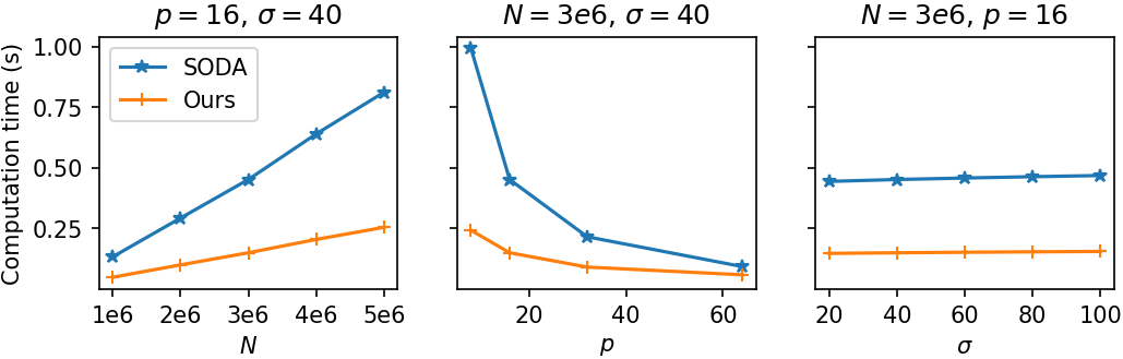
Figure 4: Computation time of $\mathtt{OPartition}$ varying input size $N$, number of servers $p$, or security parameter $\sigma$.

Primary key join (PK join)

We conducted the PK join experiments on the well-known TPC-H dataset evaluating our Algorithm 4 against Opaque’s PK join and SODA’s join using the query below:

⬇

SELECT * FROM orders JOIN customer ON o_custkey$\,=\,$c_custkey;

Note that c_custkey is the primary key of table customer, so the query is a PK join. Both tables were generated by the code from a publicly accessible GitHub repository [58] with a scale factor of 10 and with the orders table exhibiting four distinct values of Zipfian distribution parameters, denoted by $z$, as outlined in Table 3. Irrelevant columns were eliminated from computation, leaving only c_custkey, c_nationkey, o_orderkey, and o_custkey.

Table 3: PK join input table information; Total time and communication cost of the PK join algorithms

	customer		orders
#Rows	$N_{2}=1.5\!\times\!10^{6}$		$N_{1}=1.5\!\times\!10^{7}$
Zipf parameter $z$	0		0	0.5	1	1.5
Max degree $\alpha$	1		37	449	50697	210490
	Ours	Opaque	SODA
#Output ($\times 10^{7}$)	1.50	1.50	1.50	1.50	1.58	1.84
Total time (s)	6.44	12.5	11.0	11.0	11.3	12.0
Comm. cost (GB)	0.62	1.56	1.19	1.19	1.23	1.34

The results are also in Table 3. Different values of $z$ result in different maximum degrees on the join key, thereby affecting the output size of SODA’s join but not impacting our algorithm or Opaque’s join. In terms of overall running time, our algorithm improves upon the baselines by at least 70%. This improvement rises to more than 90% regarding communication costs. While SODA’s join slightly outperforms Opaque’s PK join, the gap narrows as $z$ increases, due to the increasing output size. Meanwhile, both Opaque’s PK join and our algorithm maintain steady performance despite varying $z$ due to obliviousness.

6.3 Performance of Join

For join, in addition to evaluating Jodes and SODA, we also conducted tests on a single server using the state-of-the-art oblivious standalone join [33], in which all data is sent to the first server that performs the standalone join locally and then sends the results to the other servers.

Varying datasets

We evaluated the join operator on Stanford Large Network Dataset Collection [35]. We selected four graphs with various $\ell_{\infty}$-skewnesses: “com-DBLP” (DBLP), “email-EuAll” (email), “com-Youtube” (Youtube), and “wiki-topcats” (wiki). More information of the four graphs are in Table 4. Each graph was converted into a relational table format with two columns, src and dst, to represent the source and destination nodes of each edge. We assessed the performance on the following self-join query designed to identify all length-2 paths within the graphs:

⬇

SELECT * FROM graph R JOIN graph S ON R.dst$\,=\,$S.src;

Table 4: Join input table information; Output sizes of the join algorithms

	DBLP	email	Youtube	wiki
#Input $N_{1}=N_{2}$	$1.0\!\times\!10^{6}$	$4.2\!\times\!10^{5}$	$2.9\!\times\!10^{6}$	$2.9\!\times\!10^{7}$
Max #dst $\alpha_{1}$	306	930	28576	3907
Max #src $\alpha_{2}$	113	7631	4256	238040
$\ell_{\infty}$-skewness $\phi$	$0.0049$	0.14	0.64	0.36
#Output $M$	$7.1\!\times\!10^{6}$	$5.0\!\times\!10^{7}$	$1.9\!\times\!10^{8}$	$2.6\!\times\!10^{9}$
#Output (SODA)	$7.7\!\times\!10^{6}$	$16\!\times\!10^{7}$	$21\!\times\!10^{8}$	$17\!\times\!10^{9}$

Figure 5(a) includes the performance results, with the y-axis represented on a logarithmic scale. For the wiki dataset, both SODA and standalone algorithm could not complete within an hour. The speed-up of Jodes compared to the standalone algorithm ranges from 4x (for small data) to 6x (for large data). In contrast, our speed-up over SODA is highly dependent on the value of $\phi$: it is 1.1x for DBLP (small $\phi$), 1.6x for email (medium $\phi$), and 6x for Youtube (large $\phi$). Specifically, for the Youtube dataset, the total time of SODA using 16 servers even exceeds that of the standalone algorithm with only one server, thus losing the advantages of distribution. With respect to communication costs, the standalone algorithm incurs the least, equivalent to only the I/O size. Jodes exhibits slightly higher communication costs than SODA for DBLP and email, but lower costs for Youtube.

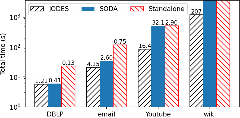
(a) Varying input datasets

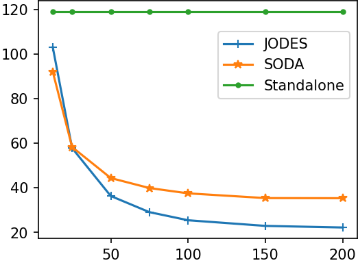
(b) Varying bandwidths (MB/s)

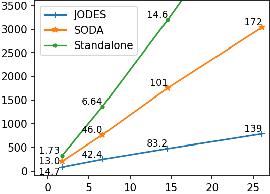
(c) Varying I/O sizes (GB)

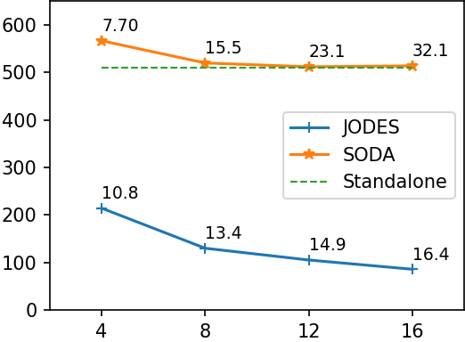
(d) Varying number of servers

Figure 5: Total time of join, where the labels on top of the bars or adjacent to the data points are communication costs (GB).

Varying bandwidths

We note that for DBLP and email in Figure 5(a), Jodes has a shorter running time but incurs a higher communication costs than SODA. The reason is that SODA adopts complex design of local computations to minimize the communication cost. To see whether SODA outperforms Jodes for limited bandwidth, we reran the tests on the email dataset and limited the bandwidth to assess its impact on performance. The results are shown in Figure 5(b). Since varying bandwidths does not change the communication costs, we only plot the running time. It appears that only under very limited bandwidth conditions (less than 25 MB/s), Jodes’s performance is surpassed by SODA. However, we argue that in distributed settings, a large bandwidth requirement is reasonable. For example, all instances of Amazon EMR [50] have a minimum bandwidth of 10 Gbps (1280 MB/s).

Varying I/O sizes

We also conducted experiments on sampled data from the wiki dataset to assess the scalability of Jodes and SODA. Specifically, we sampled each row of the input table with probability $\epsilon$ independently and then performed the join on the sampled table, as described by the following SQL:

⬇

WITH sampled AS (SELECT * FROM graph WHERE rand() < $\epsilon$)

SELECT * FROM sampled R JOIN sampled S ON R.dst$\,=\,$S.src;

Note that a sampling probability of $\epsilon$ induces the expected join size of the sampled table to be $\epsilon^{2}$ times that of the original table. We tried $\epsilon\in\{0.2,0.4,0.6,0.8\}$, and the performance results are shown in Figure 5(c). For $\epsilon=0.8$, the standalone algorithm could not finish in an hour. The total time of all algorithms scales almost linearly to the I/O sizes, i.e., the total sizes of input and output. The speed-up factor of Jodes to SODA ranges from 2.5 ($\epsilon=0.2)$ to 3.9 ($\epsilon=0.8$). Jodes also incurs less communication cost, except when $\epsilon=0.2$, where it is slightly higher.

Varying number of servers

To examine how the number of servers influences performance, we conducted experiments with different values of $p$ using the Youtube dataset, and the results are presented in Figure 5(d). We observe that SODA does not scale well for large $p$: the running time when using 12 servers is almost identical to that when using 16 servers. The major reason is that the output size of SODA on each server is $M(1/p+\phi)$. Since the extra padding size $M\phi$ is independent of $p$ and dominates the join size $M/p$, increasing the number of servers does not significantly reduce the workload on each server, while the increasing total communication can even degrade the performance. On the contrary, the output size of Jodes on each server is always $M/p$, allowing it to scale much more effectively.

Running time breakdown analysis

Jodes (Algorithm 6) works in a manner similar to the standalone algorithm at a high level, which can be segmented into the following three phases:

1. Preparation. This phase involves computing the degrees of join keys in both input tables and matching them through a primary key (PK) join (Lines 6–6);

2. Expansion. In this phase, both tables are expanded from size $N$ to $M$ through expansion operations (Lines 6–6);

3. Alignment. This phase focuses on aligning the two tables to ensure that the correct tuples match (Lines 6–6).

We evaluated the breakdown of running time for these three phases using the YouTube dataset, and the results are presented in Table 5. The findings align with our theoretical analysis, indicating that the preparation phase depends solely on $N$, while both the expansion and alignment phases are influenced by $M$, where $M\gg N$. Utilizing 16 servers, the performance improvement factors of Jodes compared to the standalone algorithm for the three phases are 5.2, 3.5, and 7.7, respectively. This suggests that optimizing the design of the expansion algorithm could be a productive pathway for further enhancing Jodes.

Table 5: Running time breakdown of Jodes and the standalone algorithm

	Preparation	Expansion	Alignment	Total
Jodes	5.7%	37.2%	57.1%	100%
Standalone	29.5%	129.7%	437.9%	597%

7 Related Work

Existing analytic systems based on TEE include [4, 19, 60, 25, 52, 54, 37]. However, most of them only focus on the standalone setting. Ohrimenko et al. [43] firstly pointed out the leakage by the network traffic in the distributed setting. Their empirical analysis on datasets that include personal and geographical data shows that the runs of typical jobs can infer precise information about their input. To prevent such leakage, they provided a shuffle-in-the middle solution: before sending data (with some padding techniques) to the intended destination, permuting the input randomly among the servers in advance to remove potential skewness; Chan et al. [14] proposed a different solution based on oblivious routing, which packs data into several bins, and routes the bins to a random server through the butterfly network. Both solutions turn any non-oblivious algorithm to the oblivious counterpart. Nevertheless, the communication cost blows up by a constant factor (at least 2) only when the load of the non-oblivious algorithm is balanced, i.e., the number of elements any server received in any round is $O(R/p)$ where $R$ is the total number of elements received of all the $p$ servers. Without load balancing, the communication cost can increase by a factor of up to $p$ in the worst-case scenario. However, existing non-oblivious join algorithms, including the hash join and sort merge join adopted by Spark [59], do not satisfy the constraint. Note that even in the plaintext model where obliviousness is not required, such imbalance happens when the input is skewed, leading to severe performance downgrade. Our join algorithm Jodes naturally provides a solution to this issue caused by input skew in the plaintext model, because its performance is independent of the input and hence its skewness.

Opaque [60] proposes an encrypted distributed analytic system based on Spark. Unlike these general solutions, it designs specialized oblivious algorithms for sorting, filter, aggregate, and PK join, but not (general equi-)join. Most of their designs are based on its oblivious sorting, which is implemented based on column sort. SODA [38] considers column sort to be heavy, so it proposes its own oblivious algorithms for filter, aggregate, and join without relying on oblivious sorting, but SODA’s join needs to publicize the maximum degrees of the input tables.

A circuit also naturally induces an oblivious algorithm in the distributed setting. To evaluate the circuit, it is necessary to ensure the inputs of each gate lie on the same server. Therefore, it incurs a communication round before each level, hence the number of rounds of the algorithm is linear to the depth of the circuit. However, existing circuits for database joins are all with $\Omega(\log^{2}N)$ depth [56, 33] and hence will induce algorithms with polylogarithm number of communication rounds, which severely downgrades the performance due to network latency. Meanwhile, common distributed algorithms introduced above incur only $O(1)$ communication rounds.

Plaintext distributed join

Numerous studies have been conducted on join algorithms within the plaintext distributed model, as referenced in [13, 32, 28, 29, 27]. These studies primarily focus on the massively parallel computation model where only the sizes of data received are considered, while disregarding the costs of sending data (including emitting the output) and local computations. However, these algorithms are unsuitable for cloud-based encrypted systems because their local computations, when made oblivious, incur costs that are significantly higher than negligible. Furthermore, the sizes of local joins in their final rounds are data-dependent, which presents challenges for adapting them into oblivious algorithms.

Join under MPC

There are several join algorithms [41, 10, 39, 8, 26, 55, 45] under the secure multi-party computation (MPC) model, in which several servers jointly compute the join over the secret shared data from the user. The security guarantee of MPC is incomparable to the distributed TEE model: Under MPC, the user does not need to trust any hardware as in TEE, but they believe that the servers will not collude to steal data from the user. In real-world scenarios, the servers in distributed TEE can belong to the same cluster connected by network with low latency and high bandwidth, while servers in MPC are usually from different organizations (e.g., Alibaba, Amazon, and Azure). Regarding efficiency, the speed of join under MPC is usually slower than the one in the standalone TEE setting, which is slower than the distributed TEE setting, All existing join algorithms under MPC incur both computation and communication cost $\Omega(N\log N+M)$ with a considerable hidden constant factor.

8 Conclusion and Future Work

We have proposed Jodes, an oblivious algorithm in the distributed setting that is superior to existing works in both theoretical and experimental aspects. Following the idea in [30], one can prove that the communication cost of a perfect load balanced oblivious join (i.e., each server holds $O(M/p)$ of the output tuples of join result) is $\Omega(N+\sqrt{Mp})$. Since the communication costs of existing oblivious join algorithms are all $\Omega(N+M)$, an interesting future research direction is to close the gap, i.e., either proposing an oblivious join algorithm with less cost or providing a stronger lower bound.

References

- Afrati and Ullman [2011] Foto N. Afrati and Jeffrey D. Ullman. Optimizing multiway joins in a map-reduce environment. IEEE Transactions on Knowledge and Data Engineering, 23(9):1282–1298, 2011. doi: 10.1109/TKDE.2011.47.
- Aggarwal and Vitter [1988] Alok Aggarwal and S. Vitter, Jeffrey. The input/output complexity of sorting and related problems. Commun. ACM, 31(9):1116–1127, sep 1988. ISSN 0001-0782. doi: 10.1145/48529.48535. URL https://doi.org/10.1145/48529.48535.
- Ajtai et al. [1983] M. Ajtai, J. Komlós, and E. Szemerédi. An 0(n log n) sorting network. In Proceedings of the Fifteenth Annual ACM Symposium on Theory of Computing, STOC ’83, page 1–9, New York, NY, USA, 1983. Association for Computing Machinery. ISBN 0897910990. doi: 10.1145/800061.808726. URL https://doi.org/10.1145/800061.808726.
- Antonopoulos et al. [2020] Panagiotis Antonopoulos, Arvind Arasu, Kunal D. Singh, Ken Eguro, Nitish Gupta, Rajat Jain, Raghav Kaushik, Hanuma Kodavalla, Donald Kossmann, Nikolas Ogg, Ravi Ramamurthy, Jakub Szymaszek, Jeffrey Trimmer, Kapil Vaswani, Ramarathnam Venkatesan, and Mike Zwilling. Azure sql database always encrypted. In Proceedings of the 2020 ACM SIGMOD International Conference on Management of Data, SIGMOD ’20, page 1511–1525, New York, NY, USA, 2020. Association for Computing Machinery. ISBN 9781450367356. doi: 10.1145/3318464.3386141. URL https://doi.org/10.1145/3318464.3386141.
- Arasu and Kaushik [2014] Arvind Arasu and Raghav Kaushik. Oblivious query processing. In Nicole Schweikardt, Vassilis Christophides, and Vincent Leroy, editors, Proc. 17th International Conference on Database Theory (ICDT), Athens, Greece, March 24-28, 2014, pages 26–37. OpenProceedings.org, 2014. doi: 10.5441/002/ICDT.2014.07. URL https://doi.org/10.5441/002/icdt.2014.07.
- Arasu et al. [2013] Arvind Arasu, Spyros Blanas, Ken Eguro, Manas Joglekar, Raghav Kaushik, Donald Kossmann, Ravi Ramamurthy, Prasang Upadhyaya, and Ramarathnam Venkatesan. Secure database-as-a-service with cipherbase. In Proceedings of the 2013 ACM SIGMOD International Conference on Management of Data, SIGMOD ’13, page 1033–1036, New York, NY, USA, 2013. Association for Computing Machinery. ISBN 9781450320375. doi: 10.1145/2463676.2467797. URL https://doi.org/10.1145/2463676.2467797.
- Asharov et al. [2020] Gilad Asharov, TH Hubert Chan, Kartik Nayak, Rafael Pass, Ling Ren, and Elaine Shi. Bucket oblivious sort: An extremely simple oblivious sort. In Symposium on Simplicity in Algorithms, pages 8–14. SIAM, 2020. doi: 10.1137/1.9781611976014.2. URL https://epubs.siam.org/doi/abs/10.1137/1.9781611976014.2.
- Badrinarayanan et al. [2022] Saikrishna Badrinarayanan, Sourav Das, Gayathri Garimella, Srinivasan Raghuraman, and Peter Rindal. Secret-shared joins with multiplicity from aggregation trees. In Proceedings of the 2022 ACM SIGSAC Conference on Computer and Communications Security, page 209–222. Association for Computing Machinery, 2022.
- Batcher [1968] K. E. Batcher. Sorting networks and their applications. In Proceedings of the April 30–May 2, 1968, Spring Joint Computer Conference, AFIPS ’68 (Spring), page 307–314, New York, NY, USA, 1968. Association for Computing Machinery. ISBN 9781450378970. doi: 10.1145/1468075.1468121. URL https://doi.org/10.1145/1468075.1468121.
- Bater et al. [2017] Johes Bater, Gregory Elliott, Craig Eggen, Satyender Goel, Abel Kho, and Jennie Rogers. Smcql: Secure querying for federated databases. Proc. VLDB Endow., 10(6):673–684, feb 2017. ISSN 2150-8097. doi: 10.14778/3055330.3055334. URL https://doi.org/10.14778/3055330.3055334.
- Bater et al. [2018] Johes Bater, Xi He, William Ehrich, Ashwin Machanavajjhala, and Jennie Rogers. Shrinkwrap: Efficient sql query processing in differentially private data federations. Proc. VLDB Endow., 12(3):307–320, nov 2018. ISSN 2150-8097. doi: 10.14778/3291264.3291274. URL https://doi.org/10.14778/3291264.3291274.
- Beame et al. [2014] Paul Beame, Paraschos Koutris, and Dan Suciu. Skew in parallel query processing. In Proceedings of the 33rd ACM SIGMOD-SIGACT-SIGART Symposium on Principles of Database Systems, PODS ’14, page 212–223, New York, NY, USA, 2014. Association for Computing Machinery. ISBN 9781450323758. doi: 10.1145/2594538.2594558. URL https://doi.org/10.1145/2594538.2594558.
- Beame et al. [2017] Paul Beame, Paraschos Koutris, and Dan Suciu. Communication steps for parallel query processing. J. ACM, 64(6), oct 2017. ISSN 0004-5411. doi: 10.1145/3125644. URL https://doi.org/10.1145/3125644.
- Chan et al. [2020] T-H. Hubert Chan, Kai-Min Chung, Wei-Kai Lin, and Elaine Shi. MPC for MPC: Secure Computation on a Massively Parallel Computing Architecture. In Thomas Vidick, editor, 11th Innovations in Theoretical Computer Science Conference (ITCS 2020), volume 151 of Leibniz International Proceedings in Informatics (LIPIcs), pages 75:1–75:52, Dagstuhl, Germany, 2020. Schloss Dagstuhl–Leibniz-Zentrum fuer Informatik. ISBN 978-3-95977-134-4. doi: 10.4230/LIPIcs.ITCS.2020.75. URL https://drops.dagstuhl.de/opus/volltexte/2020/11760.
- Chang et al. [2022] Zhao Chang, Dong Xie, Sheng Wang, and Feifei Li. Towards practical oblivious join. In Proceedings of the 2022 International Conference on Management of Data, SIGMOD ’22, page 803–817, New York, NY, USA, 2022. Association for Computing Machinery. ISBN 9781450392495. doi: 10.1145/3514221.3517868. URL https://doi.org/10.1145/3514221.3517868.
- Dean and Ghemawat [2008] Jeffrey Dean and Sanjay Ghemawat. Mapreduce: Simplified data processing on large clusters. Commun. ACM, 51(1):107–113, jan 2008. ISSN 0001-0782. doi: 10.1145/1327452.1327492. URL https://doi.org/10.1145/1327452.1327492.
- Dwork and Roth [2014] Cynthia Dwork and Aaron Roth. The algorithmic foundations of differential privacy. Found. Trends Theor. Comput. Sci., 9(3–4):211–407, aug 2014. ISSN 1551-305X. doi: 10.1561/0400000042. URL https://doi.org/10.1561/0400000042.
- El-Hindi et al. [2022] Muhammad El-Hindi, Tobias Ziegler, Matthias Heinrich, Adrian Lutsch, Zheguang Zhao, and Carsten Binnig. Benchmarking the second generation of intel sgx hardware. DaMoN ’22, New York, NY, USA, 2022. Association for Computing Machinery. ISBN 9781450393782. doi: 10.1145/3533737.3535098. URL https://doi.org/10.1145/3533737.3535098.
- Eskandarian and Zaharia [2019] Saba Eskandarian and Matei Zaharia. Oblidb: Oblivious query processing for secure databases. Proc. VLDB Endow., 13(2):169–183, oct 2019. ISSN 2150-8097. doi: 10.14778/3364324.3364331. URL https://doi.org/10.14778/3364324.3364331.
- Evans et al. [2018] David Evans, Vladimir Kolesnikov, and Mike Rosulek. A pragmatic introduction to secure multi-party computation. Found. Trends Priv. Secur., 2(2–3):70–246, dec 2018. ISSN 2474-1558. doi: 10.1561/3300000019. URL https://doi.org/10.1561/3300000019.
- Facebook [2022] Facebook. Proxygen: Facebook’s c++ http libraries, 2022. URL https://github.com/facebook/proxygen/releases/tag/v2022.11.14.00.
- Goldreich and Ostrovsky [1996] Oded Goldreich and Rafail Ostrovsky. Software protection and simulation on oblivious rams. J. ACM, 43(3):431–473, may 1996. ISSN 0004-5411. doi: 10.1145/233551.233553. URL https://doi.org/10.1145/233551.233553.
- Goodrich [2014] Michael T. Goodrich. Zig-zag sort: A simple deterministic data-oblivious sorting algorithm running in o(n log n) time. In Proceedings of the Forty-Sixth Annual ACM Symposium on Theory of Computing, STOC ’14, page 684–693, New York, NY, USA, 2014. Association for Computing Machinery. ISBN 9781450327107. doi: 10.1145/2591796.2591830. URL https://doi.org/10.1145/2591796.2591830.
- Goodrich et al. [2011] Michael T. Goodrich, Nodari Sitchinava, and Qin Zhang. Sorting, searching, and simulation in the mapreduce framework. In Takao Asano, Shin-ichi Nakano, Yoshio Okamoto, and Osamu Watanabe, editors, Algorithms and Computation, pages 374–383, Berlin, Heidelberg, 2011. Springer Berlin Heidelberg. ISBN 978-3-642-25591-5.
- Gribov et al. [2017] Alexey Gribov, Dhinakaran Vinayagamurthy, and Sergey Gorbunov. Stealthdb: a scalable encrypted database with full sql query support. Proceedings on Privacy Enhancing Technologies, 2019:370 – 388, 2017. URL https://api.semanticscholar.org/CorpusID:28591687.
- Han et al. [2022] Feng Han, Lan Zhang, Hanwen Feng, Weiran Liu, and Xiang-Yang Li. Scape: Scalable collaborative analytics system on private database with malicious security. In 38th IEEE International Conference on Data Engineering, ICDE 2022, Kuala Lumpur, Malaysia, May 9-12, 2022, pages 1740–1753. IEEE, 2022. doi: 10.1109/ICDE53745.2022.00176. URL https://doi.org/10.1109/ICDE53745.2022.00176.
- Hu [2021] Xiao Hu. Cover or pack: New upper and lower bounds for massively parallel joins. In Proceedings of the 40th ACM SIGMOD-SIGACT-SIGAI Symposium on Principles of Database Systems, PODS’21, page 181–198, New York, NY, USA, 2021. Association for Computing Machinery. ISBN 9781450383813. doi: 10.1145/3452021.3458319. URL https://doi.org/10.1145/3452021.3458319.
- Hu and Yi [2019] Xiao Hu and Ke Yi. Instance and output optimal parallel algorithms for acyclic joins. In Proceedings of the 38th ACM SIGMOD-SIGACT-SIGAI Symposium on Principles of Database Systems, PODS ’19, page 450–463, New York, NY, USA, 2019. Association for Computing Machinery. ISBN 9781450362276. doi: 10.1145/3294052.3319698. URL https://doi.org/10.1145/3294052.3319698.
- Hu and Yi [2020] Xiao Hu and Ke Yi. Parallel algorithms for sparse matrix multiplication and join-aggregate queries. In Proceedings of the 39th ACM SIGMOD-SIGACT-SIGAI Symposium on Principles of Database Systems, PODS’20, page 411–425, New York, NY, USA, 2020. Association for Computing Machinery. ISBN 9781450371087. doi: 10.1145/3375395.3387657. URL https://doi.org/10.1145/3375395.3387657.
- Hu et al. [2017] Xiao Hu, Yufei Tao, and Ke Yi. Output-optimal parallel algorithms for similarity joins. In Proceedings of the 36th ACM SIGMOD-SIGACT-SIGAI Symposium on Principles of Database Systems, PODS ’17, page 79–90, New York, NY, USA, 2017. Association for Computing Machinery. ISBN 9781450341981. doi: 10.1145/3034786.3056110. URL https://doi.org/10.1145/3034786.3056110.
- Islam et al. [2012] Mohammad Saiful Islam, Mehmet Kuzu, and Murat Kantarcioglu. Access pattern disclosure on searchable encryption: Ramification, attack and mitigation. In 19th Annual Network and Distributed System Security Symposium, NDSS 2012, San Diego, California, USA, February 5-8, 2012. The Internet Society, 2012. URL https://www.ndss-symposium.org/ndss2012/access-pattern-disclosure-searchable-encryption-ramification-attack-and-mitigation.
- Ketsman and Suciu [2017] Bas Ketsman and Dan Suciu. A worst-case optimal multi-round algorithm for parallel computation of conjunctive queries. In Proceedings of the 36th ACM SIGMOD-SIGACT-SIGAI Symposium on Principles of Database Systems, PODS ’17, page 417–428, New York, NY, USA, 2017. Association for Computing Machinery. ISBN 9781450341981. doi: 10.1145/3034786.3034788. URL https://doi.org/10.1145/3034786.3034788.
- Krastnikov et al. [2020] Simeon Krastnikov, Florian Kerschbaum, and Douglas Stebila. Efficient oblivious database joins. Proc. VLDB Endow., 13(12):2132–2145, jul 2020. ISSN 2150-8097. doi: 10.14778/3407790.3407814. URL https://doi.org/10.14778/3407790.3407814.
- Leighton [1984] Tom Leighton. Tight bounds on the complexity of parallel sorting. In Proceedings of the Sixteenth Annual ACM Symposium on Theory of Computing, STOC ’84, page 71–80, New York, NY, USA, 1984. Association for Computing Machinery. ISBN 0897911334. doi: 10.1145/800057.808667. URL https://doi.org/10.1145/800057.808667.
- Leskovec and Krevl [2014] Jure Leskovec and Andrej Krevl. SNAP Datasets: Stanford large network dataset collection. http://snap.stanford.edu/data, June 2014.
- Li et al. [2023a] Mingyu Li, Xuyang Zhao, Le Chen, Cheng Tan, Huorong Li, Sheng Wang, Zeyu Mi, Yubin Xia, Feifei Li, and Haibo Chen. Encrypted databases made secure yet maintainable. In 17th USENIX Symposium on Operating Systems Design and Implementation (OSDI 23), pages 117–133, Boston, MA, July 2023a. USENIX Association. ISBN 978-1-939133-34-2. URL https://www.usenix.org/conference/osdi23/presentation/li-mingyu.
- Li et al. [2023b] Xiang Li, Fabing Li, and Mingyu Gao. Flare: A fast, secure, and memory-efficient distributed analytics framework. Proc. VLDB Endow., 16(6):1439–1452, feb 2023b. ISSN 2150-8097. doi: 10.14778/3583140.3583158. URL https://doi.org/10.14778/3583140.3583158.
- Li et al. [2023c] Xiang Li, Nuozhou Sun, Yunqian Luo, and Mingyu Gao. Soda: A set of fast oblivious algorithms in distributed secure data analytics. Proc. VLDB Endow., 16(7):1671–1684, mar 2023c. ISSN 2150-8097. doi: 10.14778/3587136.3587142. URL https://doi.org/10.14778/3587136.3587142.
- Liagouris et al. [2023] John Liagouris, Vasiliki Kalavri, Muhammad Faisal, and Mayank Varia. SECRECY: secure collaborative analytics in untrusted clouds. In Mahesh Balakrishnan and Manya Ghobadi, editors, 20th USENIX Symposium on Networked Systems Design and Implementation, NSDI 2023, Boston, MA, April 17-19, 2023, pages 1031–1056. USENIX Association, 2023.
- Mitzenmacher and Upfal [2005] Michael Mitzenmacher and Eli Upfal. Probability and Computing: Randomized Algorithms and Probabilistic Analysis. Cambridge University Press, USA, 2005. ISBN 0521835402.
- Mohassel et al. [2020] Payman Mohassel, Peter Rindal, and Mike Rosulek. Fast database joins and psi for secret shared data. In Proceedings of the 2020 ACM SIGSAC Conference on Computer and Communications Security, page 1271–1287. Association for Computing Machinery, 2020.
- Ngai et al. [2024] N. Ngai, I. Demertzis, J. Ghareh Chamani, and D. Papadopoulos. Distributed & scalable oblivious sorting and shuffling. In 2024 IEEE Symposium on Security and Privacy (SP), pages 156–156, Los Alamitos, CA, USA, may 2024. IEEE Computer Society. doi: 10.1109/SP54263.2024.00153. URL https://doi.ieeecomputersociety.org/10.1109/SP54263.2024.00153.
- Ohrimenko et al. [2015] Olga Ohrimenko, Manuel Costa, Cédric Fournet, Christos Gkantsidis, Markulf Kohlweiss, and Divya Sharma. Observing and preventing leakage in mapreduce. In Proceedings of the 22nd ACM SIGSAC Conference on Computer and Communications Security, CCS ’15, page 1570–1581, New York, NY, USA, 2015. Association for Computing Machinery. ISBN 9781450338325. doi: 10.1145/2810103.2813695. URL https://doi.org/10.1145/2810103.2813695.
- Ohrimenko et al. [2016] Olga Ohrimenko, Felix Schuster, Cédric Fournet, Aastha Mehta, Sebastian Nowozin, Kapil Vaswani, and Manuel Costa. Oblivious multi-party machine learning on trusted processors. SEC’16, page 619–636, USA, 2016. USENIX Association. ISBN 9781931971324.
- Poddar et al. [2021] Rishabh Poddar, Sukrit Kalra, Avishay Yanai, Ryan Deng, Raluca Ada Popa, and Joseph M. Hellerstein. Senate: A Maliciously-Secure MPC platform for collaborative analytics. In 30th USENIX Security Symposium (USENIX Security 21), pages 2129–2146. USENIX Association, August 2021. ISBN 978-1-939133-24-3. URL https://www.usenix.org/conference/usenixsecurity21/presentation/poddar.
- Popa et al. [2011] Raluca Ada Popa, Catherine M. S. Redfield, Nickolai Zeldovich, and Hari Balakrishnan. Cryptdb: Protecting confidentiality with encrypted query processing. In Proceedings of the Twenty-Third ACM Symposium on Operating Systems Principles, SOSP ’11, page 85–100, New York, NY, USA, 2011. Association for Computing Machinery. ISBN 9781450309776. doi: 10.1145/2043556.2043566. URL https://doi.org/10.1145/2043556.2043566.
- Priebe et al. [2018] Christian Priebe, Kapil Vaswani, and Manuel Costa. Enclavedb: A secure database using sgx. In 2018 IEEE Symposium on Security and Privacy (SP), pages 264–278, 2018. doi: 10.1109/SP.2018.00025.
- Ren et al. [2022] Xuanle Ren, Le Su, Zhen Gu, Sheng Wang, Feifei Li, Yuan Xie, Song Bian, Chao Li, and Fan Zhang. Heda: Multi-attribute unbounded aggregation over homomorphically encrypted database. Proc. VLDB Endow., 16(4):601–614, dec 2022. ISSN 2150-8097. doi: 10.14778/3574245.3574248. URL https://doi.org/10.14778/3574245.3574248.
- Sasy et al. [2022] Sajin Sasy, Aaron Johnson, and Ian Goldberg. Fast fully oblivious compaction and shuffling. In Proceedings of the 2022 ACM SIGSAC Conference on Computer and Communications Security, CCS ’22, page 2565–2579, New York, NY, USA, 2022. Association for Computing Machinery. ISBN 9781450394505. doi: 10.1145/3548606.3560603. URL https://doi.org/10.1145/3548606.3560603.
- Services [2024] Amazon Web Services. Amazon emr pricing, 2024. URL https://aws.amazon.com/emr/pricing/. Accessed: 2024-08-12.
- Stefanov et al. [2018] Emil Stefanov, Marten Van Dijk, Elaine Shi, T.-H. Hubert Chan, Christopher Fletcher, Ling Ren, Xiangyao Yu, and Srinivas Devadas. Path oram: An extremely simple oblivious ram protocol. J. ACM, 65(4), apr 2018. ISSN 0004-5411. doi: 10.1145/3177872. URL https://doi.org/10.1145/3177872.
- Sun et al. [2021] Yuanyuan Sun, Sheng Wang, Huorong Li, and Feifei Li. Building enclave-native storage engines for practical encrypted databases. Proc. VLDB Endow., 14(6):1019–1032, feb 2021. ISSN 2150-8097. doi: 10.14778/3447689.3447705. URL https://doi.org/10.14778/3447689.3447705.
- Valiant [1990] Leslie G. Valiant. A bridging model for parallel computation. Commun. ACM, 33(8):103–111, aug 1990. ISSN 0001-0782. doi: 10.1145/79173.79181. URL https://doi.org/10.1145/79173.79181.
- Wang et al. [2022] Sheng Wang, Yiran Li, Huorong Li, Feifei Li, Chengjin Tian, Le Su, Yanshan Zhang, Yubing Ma, Lie Yan, Yuanyuan Sun, Xuntao Cheng, Xiaolong Xie, and Yu Zou. Operon: An encrypted database for ownership-preserving data management. Proc. VLDB Endow., 15(12):3332–3345, aug 2022. ISSN 2150-8097. doi: 10.14778/3554821.3554826. URL https://doi.org/10.14778/3554821.3554826.
- Wang and Yi [2021] Yilei Wang and Ke Yi. Secure yannakakis: Join-aggregate queries over private data. In Proceedings of the 2021 International Conference on Management of Data, SIGMOD ’21, page 1969–1981, New York, NY, USA, 2021. Association for Computing Machinery. ISBN 9781450383431. doi: 10.1145/3448016.3452808. URL https://doi.org/10.1145/3448016.3452808.
- Wang and Yi [2022] Yilei Wang and Ke Yi. Query evaluation by circuits. PODS ’22, page 67–78, New York, NY, USA, 2022. Association for Computing Machinery. ISBN 9781450392600. doi: 10.1145/3517804.3524142. URL https://doi.org/10.1145/3517804.3524142.
- Xu et al. [2015] Yuanzhong Xu, Weidong Cui, and Marcus Peinado. Controlled-channel attacks: Deterministic side channels for untrusted operating systems. In Proceedings of the 2015 IEEE Symposium on Security and Privacy, SP ’15, page 640–656, USA, 2015. IEEE Computer Society. ISBN 9781467369497. doi: 10.1109/SP.2015.45. URL https://doi.org/10.1109/SP.2015.45.
- YSU-Data-Lab [2024] YSU-Data-Lab. Tpc-h-skew, 2024. URL https://github.com/YSU-Data-Lab/TPC-H-Skew. Accessed: 2024-08-12.
- Zaharia et al. [2012] Matei Zaharia, Mosharaf Chowdhury, Tathagata Das, Ankur Dave, Justin Ma, Murphy McCauley, Michael J. Franklin, Scott Shenker, and Ion Stoica. Resilient distributed datasets: A fault-tolerant abstraction for in-memory cluster computing. In Proceedings of the 9th USENIX Conference on Networked Systems Design and Implementation, NSDI’12, page 2, USA, 2012. USENIX Association.
- Zheng et al. [2017] Wenting Zheng, Ankur Dave, Jethro G. Beekman, Raluca Ada Popa, Joseph E. Gonzalez, and Ion Stoica. Opaque: An oblivious and encrypted distributed analytics platform. In Proceedings of the 14th USENIX Conference on Networked Systems Design and Implementation, NSDI’17, page 283–298, USA, 2017. USENIX Association. ISBN 9781931971379.
- Zhu et al. [2021] Jinwei Zhu, Kun Cheng, Jiayang Liu, and Liang Guo. Full encryption: An end to end encryption mechanism in gaussdb. Proc. VLDB Endow., 14(12):2811–2814, jul 2021. ISSN 2150-8097. doi: 10.14778/3476311.3476351. URL https://doi.org/10.14778/3476311.3476351.
- Zhuang et al. [2004] Xiaotong Zhuang, Tao Zhang, and Santosh Pande. Hide: an infrastructure for efficiently protecting information leakage on the address bus. SIGARCH Comput. Archit. News, 32(5):72–84, oct 2004. ISSN 0163-5964. doi: 10.1145/1037947.1024403. URL https://doi.org/10.1145/1037947.1024403.