Prompt-CAM: A Simpler Interpretable Transformer for Fine-Grained Analysis

Abstract

We present a simple usage of pre-trained Vision Transformers (ViTs) for fine-grained analysis, aiming to identify and localize the traits that distinguish visually similar categories, such as different bird species or dog breeds. Pre-trained ViTs such as DINO have shown remarkable capabilities to extract localized, informative features. However, using saliency maps like Grad-CAM can hardly point out the traits: they often locate the whole object by a blurred, coarse heatmap, not traits. We propose a novel approach Prompt Class Attention Map (Prompt-CAM) to the rescue. Prompt-CAM learns class-specific prompts to a pre-trained ViT and uses the corresponding outputs for classification. To classify an image correctly, the true-class prompt must attend to the unique image patches not seen in other classes’ images, i.e., traits. As such, the true class’s multi-head attention maps reveal traits and their locations. Implementation-wise, Prompt-CAM is almost a free lunch by simply modifying the prediction head of Visual Prompt Tuning (VPT). This makes Prompt-CAM fairly easy to train and apply, sharply contrasting other interpretable methods that design specific models and training processes. It is even simpler than the recently published INterpretable TRansformer (INTR), whose encoder-decoder architecture prevents it from leveraging pre-trained ViTs. Extensive empirical studies on a dozen datasets from various domains (e.g., birds, fishes, insects, fungi, flowers, food, and cars) validate Prompt-CAM superior interpretation capability.

1 Introduction

Vision Transformers (ViT) [9] pre-trained on huge datasets have greatly improved vision recognition, even for fine-grained objects [46, 39, 51, 10]. DINO [4] and DINOv2 [28] further showed remarkable abilities to extract features that are localized and informative, precisely representing the corresponding coordinates in the input image. These advancements open up the possibility of using pre-trained ViTs to discover “traits” that highlight each category’s identity and distinguish it from other visually close ones.

One popular approach to this is saliency maps, for example, Class Activation Map (CAM) [50, 36, 24, 13]. After extracting the feature maps from an image, CAM highlights the spatial grids whose feature vectors align with the target class’s fully connected weight. While easy to implement and efficient, the reported CAM saliency on ViTs is often far from expectation. It frequently locates the whole object with a blurred, coarse heatmap, instead of focusing on subtle traits that tell visually similar objects (e.g., birds) apart. One may argue that CAM was not originally developed for ViTs, but even with dedicated variants like attention rollout [14, 5, 1], the issue is only mildly attenuated.

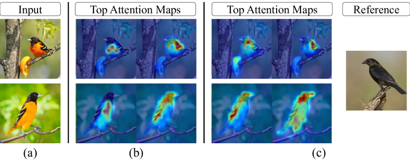
Figure 1: Prompt-CAM identifies and localizes traits class-specifically and consistently. (a) Images of “Baltimore Oriole.” (b) Top-2 “Baltimore Oriole”-specific attention maps (across 12 heads) using Prompt-CAM, focusing on the orange belly and black wings. (c) Top-2 “Bronzed Cowbird”-specific attention maps on the same images, focusing on the black wings and heads.

What if we look at the attention maps? ViTs rely on self-attention to relate image patches; the [CLS] token aggregates image features by attending to informative patches. As shown in [7, 38, 26], the attention maps of the [CLS] token do highlight local regions inside the object. However, these regions are not “class-specific.” Instead, they often point to the same object regions across different categories, such as body parts like heads, wings, and tails of bird species. While these are where traits usually reside, they are not traits. For example, the distinction between “Red-winged Blackbird” and other bird species is the red spot on the wing, having little to do with other body parts.

How can we leverage pre-trained ViTs, particularly their localized and informative patch features, to identify traits that are so special for each category?

Our proposal is to prompt the ViTs with learnable “class-specific” tokens, one for each class, inspired by [30, 19, 48]. These “class-specific” tokens, once inputted to ViTs, attend to image patches via self-attention, just like the [CLS] token. Yet, unlike [CLS] token which is “class-agnostic,” these “class-specific” tokens can attend to the same image differently, having the potential to highlight local regions that are specific to the corresponding classes, i.e., traits.

We implement our approach, which we name Prompt Class Attention Map (Prompt-CAM), as follows. Given a pre-trained ViT and a fine-grained classification dataset with $C$ classes, we add $C$ learnable tokens as extra inputs to the first Transformer layer. To make these tokens “class-specific,” we collect their corresponding output vectors after the final Transformer layer and perform inner products with a shared vector (also learnable) to obtain $C$ “class-specific” scores, following [30]. One may interpret each class-specific score as how clearly the corresponding class’s traits are seen in the input image. Intuitively, the input image’s ground-truth class should possess the highest score, and we encourage this by minimizing a cross-entropy loss, treating the scores as logits. We keep the whole pre-trained ViT frozen and only optimize the $C$ tokens and the shared scoring vector. See section 3 for details and variants.

For interpretation during inference, we input the image and the $C$ tokens simultaneously to the ViT to obtain the $C$ scores. One can then select a specific class, for example, the highest-score class, and visualize the $R$ multi-head attention maps to the image patches. (See section 3 for how to rank these $R$ maps to highlight the most discriminative traits.) When the highest-score class is the ground-truth class, the attention maps reveal its traits. Otherwise, comparing the highest-score class’s attention and the ground-truth class’s attention explains why the image is misclassified. Example reasons involve the object in the image being partially occluded or in an odd pose, such that its traits were invisible, or somehow its appearance being too similar to a wrong class, perhaps due to lighting conditions (see Figure 5).

Prompt-CAM is fairly easy to implement and train. It requires no change to pre-trained ViTs and no specially designed loss function or training strategy—just the standard cross-entropy loss and SGD. Indeed, building upon Visual Prompt Tuning (VPT) [12], one merely needs to adjust a few lines of code and can enjoy fine-grained interpretation. This simplicity sharply contrasts other interpretable methods like ProtoPNet [6] and ProtoTree [25]. Compared to INterpretable TRansformer (INTR) [30], which also featured simplicity, Prompt-CAM has three notable advantages. First, Prompt-CAM is encoder-only and can potentially take any ViT encoders. In contrast, INTR is built upon an encoder-decoder model pre-trained on object detection datasets. Thus, Prompt-CAM can leverage up-to-date pre-trained models more easily. Second, as a result, Prompt-CAM can be trained much faster—only the prompts and the shared vector need to be learned. In contrast, INTR typically demands full fine-tuning. Third, Prompt-CAM produces cleaner and sharper attention maps than INTR, which we attribute to the usages of state-of-the-art ViTs like DINO or DINOv2. Put things together, we view Prompt-CAM as a simpler yet stronger interpretable Transformer.

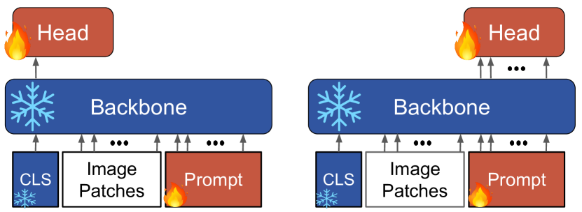
(a)              (b)

Figure 2: Prompt-CAM vs. Visual Prompt Tuning (VPT). (a) VPT [12] adds the prediction head on top of the [CLS] token’s output, a default design to use ViTs for classification. (b) Prompt-CAM adds the prediction head on top of the injected prompts’ outputs, making them class-specific to identify and localize traits.

We validate Prompt-CAM on over a dozen datasets: CUB-200-2011 [43], Birds-525 [32], Oxford Pet [29], Stanford Dogs [15], Stanford Cars [16], iNaturalist-2021-Moths [41], Fish Vista [23], Rare Species [40], Insects-2 [47], iNaturalist-2021-Fungi [41], Oxford Flowers [27], Medicinal Leaf [35], Stanford Cars [16] and Food 101 [2]. Prompt-CAM can identify different traits of a category through multi-head attention and consistently localize them in images. To our knowledge, Prompt-CAM is the only explainable or interpretable method for vision that has been evaluated on such a broad range of domains. We further show Prompt-CAM’s extendability by applying it to discovering taxonomy keys. Our contributions are two-fold.

• We present Prompt-CAM, an easily implementable, trainable, and reproducible interpretable method that leverages the representations of pre-trained ViTs to identify and localize traits for fine-grained analysis.

• We conduct extensive experiments on more than a dozen datasets to validate Prompt-CAM’s interpretation quality, wide applicability, and extendability.

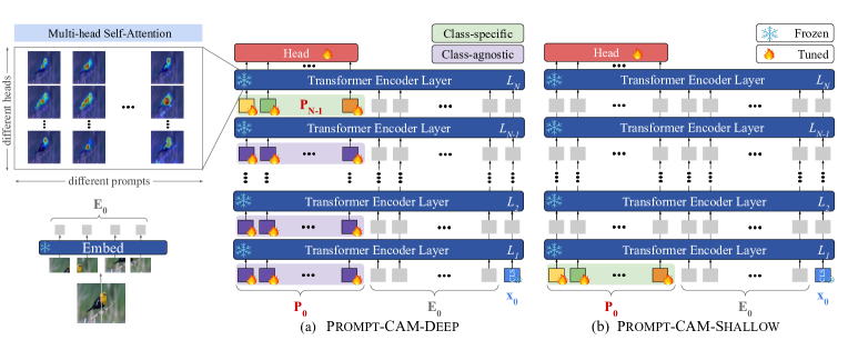
Figure 3: Overview of Prompt Class Attention Map (Prompt-CAM). We explore two variants, given a pre-trained ViT with $N$ layers and a downstream task with $C$ classes: (a) Prompt-CAM-Deep: insert $C$ learnable “class-specific” tokens to the last layer’s input and $C$ learnable “class-agnostic” tokens to each of the other $N-1$ layers’ input; (b) Prompt-CAM-Shallow: insert $C$ learnable “class-specific” tokens to the first layer’s input. During training, only the prompts and the prediction head are updated; the whole ViT is frozen.

Comparison to closely related work. Besides INTR [30], our class-specific attentions are inspired by two other works in different contexts, MCTformer for weakly supervised semantic segmentation [48] and Query2Label for multi-label classification [19]. Both of them learned class-specific tokens but aimed to localize visually distinct common objects (e.g., people, horses, and flights). In contrast, we focus on fine-grained analysis: supervised by class labels of visually similar objects (e.g., bird species), we aim to localize their traits (e.g., red spots on wings). One particular feature of Prompt-CAM is its simplicity, in both implementation and compatibility with pre-trained backbones, without extra modules, loss terms, and changes to the backbones, making it an almost plug-and-pay approach to interpretation.

2 Related Work (See the Suppl. for Details)

Seeing the remarkable performance of neural networks, researchers have strived to understand their predictions. Explainable methods do not change the neural network models but derive saliency maps or image masks to pinpoint where the model looks [36, 13, 24, 44]. Interpretable methods design specific neural networks (and training procedures) whose inner workings reveal how the model makes predicts [45, 30, 20, 49]. Prompt-CAM belongs to the interpretable methods but makes minimal changes to ViTs and can be easily trained and applied.

3 Approach

We propose Prompt Class Attention Map (Prompt-CAM) to leverage pre-trained Vision Transformers (ViTs) [9] for fine-grained analysis. The goal is to identify and localize traits that highlight an object category’s identity. Prompt-CAM adds learnable class-specific tokens to prompt ViTs, producing class-specific attention maps that reveal traits. The overall framework is presented in Figure 3. We deliberately follow the notation and naming of Visual Prompt Tuning (VPT) [12] for ease of reference.

3.1 Preliminaries

A ViT typically contains $N$ Transformer layers [42]. Each consists of a Multi-head Self-Attention (MSA) block, a Multi-Layer Perceptron (MLP) block, and several other operations like layer normalization and residual connections.

The input image $\bm{I}$ to ViTs is first divided into $M$ fixed-sized patches. Each is then projected into a $D$-dimensional feature space with positional encoding, denoted by ${\bm{e}}_{0}^{j}$, with $1\leq j\leq M$. We use $\bm{E}_{0}=[{\bm{e}}_{0}^{1},\cdots,{\bm{e}}_{0}^{M}]\in\mathbb{R}^{D\times M}$ to denote their column-wise concatenation.

Together with a learnable [CLS] token ${\bm{x}}_{0}\in\mathbb{R}^{D}$, the whole ViT is formulated as:

$$[\bm{E}_{i},{\bm{x}}_{i}]=L_{i}([\bm{E}_{i-1},{\bm{x}}_{i-1}]),\quad i=1,\cdots,N,$$

where $L_{i}$ denotes the $i$-th Transformer layer. The final ${\bm{x}}_{N}$ is typically used to represent the whole image and fed into a prediction head for classification.

3.2 Prompt Class Attention Map (Prompt-CAM)

Given a pre-trained ViT and a downstream classification dataset with $C$ classes, we introduce a set of $C$ learnable $D$-dimensional vectors to prompt the ViT. These vectors are learned to be “class-specific” by minimizing the cross-entropy loss, during which the ViT backbone is frozen. In the following, we first introduce the baseline version.

Prompt-CAM-Shallow. The $C$ class-specific prompts are injected into the first Transformer layer $L_{1}$. We denote each prompt by $\bm{p}^{c}\in\mathbb{R}^{D}$, where $1\leq c\leq C$, and use $\bm{P}=[\bm{p}^{1},\cdots,\bm{p}^{C}]\in\mathbb{R}^{D\times C}$ to indicate their column-wise concatenation. The prompted ViT is:

$$[\bm{Z}_{1},\bm{E}_{1},{\bm{x}}_{1}] =L_{1}([\bm{P},\bm{E}_{0},{\bm{x}}_{0}])$$

$$[\bm{Z}_{i},\bm{E}_{i},{\bm{x}}_{i}] =L_{i}([\bm{Z}_{i-1},\bm{E}_{i-1},{\bm{x}}_{i-1}]),\quad i=2,\cdots,N,$$

where $\bm{Z}_{i}$ represents the features corresponding to $\bm{P}$, computed by the $i$-th Transformer layer $L_{i}$. The order among ${\bm{x}}_{0}$, $\bm{E}_{0}$, and $\bm{P}$ does not matter since the positional encoding of patch locations has already been inserted into $\bm{E}_{0}$.

To make $\bm{P}=[\bm{p}^{1},\cdots,\bm{p}^{C}]$ class-specific, we employ a cross-entropy loss on top of the corresponding ViT’s output, i.e., $\bm{Z}_{N}=[{\bm{z}}_{N}^{1},\cdots,{\bm{z}}_{N}^{C}]$. Given a labeled training example $(\bm{I},y\in\{1,\cdots,C\})$, we calculate the logit of each class by:

$$s[c]=\bm{w}^{\top}{\bm{z}}_{N}^{c},\quad 1\leq c\leq C,$$ (1)

where $\bm{w}\in\mathbb{R}^{D}$ is a learnable vector. $\bm{P}$ can then be updated by minimizing the loss:

$$-\log\left(\cfrac{\exp{\left(s[y]\right)}}{\sum_{c}\exp{\left(s[c]\right)}}\right).$$ (2)

Prompt-CAM-Deep. While straightforward, Prompt-CAM-Shallow has two potential drawbacks. First, the class-specific prompts attend to every layer’s patch features, i.e., $\bm{E}_{i}$, $i=0,\cdots,N-1$. However, features of the early layers are often not informative enough but noisy for differentiating classes. Second, the prompts $\bm{p}^{1},\cdots,\bm{p}^{C}$ have a “double duty.” Individually, each needs to highlight class-specific traits. Collectively, they need to adapt pre-trained ViTs to downstream tasks, the original purpose of VPT [12]. In our case, the downstream task is a new usage of ViTs on a specific fine-grained dataset.

To address these issues, we resort to the VPT-Deep’s design while deliberately decoupling injected prompts’ roles. VPT-Deep adds learnable prompts to every layer’s input. Denote by $\bm{P}_{i-1}=[\bm{p}_{i-1}^{1},\cdots,\bm{p}_{i-1}^{C}]$ the prompts to the $i$-th Transformer layer, the deep-prompted ViT is formulated as:

$$[\bm{Z}_{i},\bm{E}_{i},{\bm{x}}_{i}] =L_{i}([\bm{P}_{i-1},\bm{E}_{i-1},{\bm{x}}_{i-1}]),\quad i=1,\cdots,N,$$ (3)

It is worth noting that the features $\bm{Z}_{i}$ after the $i$-th layer are not inputted to the next layer, and are typically disregarded.

In Prompt-CAM-Deep, we repurpose $\bm{Z}_{N}$ for classification, following Equation 1. As such, after minimizing the cross entropy loss in Equation 2, the corresponding prompts $\bm{P}_{N-1}=[\bm{p}_{N-1}^{1},\cdots,\bm{p}_{N-1}^{C}]$ will be class-specific. Prompts to the other layers’ inputs, i.e., $\bm{P}_{i}=[\bm{p}_{i}^{1},\cdots,\bm{p}_{i}^{C}]$ for $i=0,\cdots,N-2$, remain class-agnostic, because $\bm{p}_{i}^{c}$ does not particularly serve for the $c$-th class, unlike $\bm{p}_{N-1}^{c}$. In other words, Prompt-CAM-Deep learns both class-specific prompts for trait localization and class-agnostic prompts for adaptation. The class-specific prompts $\bm{P}_{N-1}$ only attend to the patch features $\bm{E}_{N-1}$ inputted to the last Transformer layer $L_{N}$, further addressing the other issue in Prompt-CAM-Shallow.

In the following, we focus on Prompt-CAM-Deep.

3.3 Trait Identification and Localization

During inference, given an image $\bm{I}$, Prompt-CAM-Deep extracts patch embeddings $\bm{E}_{0}=[{\bm{e}}_{0}^{1},\cdots,{\bm{e}}_{0}^{M}]$ and follows Equation 3 to obtain $\bm{Z}_{N}$ and Equation 1 to obtain $s[c]$ for $c\in\{1,\cdots,C\}$. The predicted label $\hat{y}$ is:

$$\hat{y}=\operatorname{arg\,max}_{c\in\{1,\cdots,C\}}s[c].$$ (4)

What are the traits of class $c$? To answer this question, one could collect images whose true and predicted classes are both class $c$ (i.e., correctly classified) and visualize the multi-head attention maps queried by $\bm{p}_{N-1}^{c}$ in layer $L_{N}$.

Specifically, in layer $L_{N}$ with $R$ attention heads, the patch features $\bm{E}_{N-1}\in\mathbb{R}^{D\times M}$ are projected into $R$ key matrices, denoted by $\bm{K}_{N-1}^{r}\in\mathbb{R}^{D^{\prime}\times M}$, $r=1,\cdots,R$. The $j$-th column corresponds to the $j$-th patch in $\bm{I}$. Meanwhile, the prompt $\bm{p}_{N-1}^{c}$ is projected into $R$ query vectors $\bm{q}_{N-1}^{c,r}\in\mathbb{R}^{D^{\prime}}$, $r=1,\cdots,R$. Queried by $\bm{p}_{N-1}^{c}$, the $r$-th head’s attention map ${\bm{\alpha}}^{c,r}_{N-1}\in\mathbb{R}^{M}$ is computed by:

$${\bm{\alpha}}^{c,r}_{N-1}=\operatorname{softmax}\left(\cfrac{{\bm{K}_{N-1}^{r}}^{\top}\bm{q}^{c,r}_{N-1}}{D^{\prime}}\right)\in\mathbb{R}^{M}.$$ (5)

Conceptually, from the $r$-th head’s perspective, the weight $\alpha^{c,r}_{N-1}[j]$ indicates how important the $j$-th patch is for classifying class $c$, hence localizing traits in the image. Ideally, each head should attend to different (sets of) patches to look for multiple traits that together highlight class $c$’s identity. By visualizing each attention map ${\bm{\alpha}}^{c,r}_{N-1}$, $r=1,\cdots,R$, instead of pooling them averagely, Prompt-CAM can potentially identify up to $R$ different traits for class $c$.

Which traits are more discriminative? For categories that are so distinctive like “Red-winged Blackbird,” a few traits are sufficient to distinguish them from others. To automatically identify these most discriminative traits, we take a greedy approach, progressively blurring the least important traits until the image is classified wrongly. The remaining ones highlight the traits that are sufficient for classification.

Suppose class $c$ is the true class and the image is correctly classified. In each greedy step, for each of the unblurred heads indexed by $r$, we iteratively replace ${\bm{\alpha}}^{c,r}_{N-1}$ with $\frac{1}{M}\textbf{1}$ and recalculate $s[c]$ in Equation 1, where $\textbf{1}\in\mathbb{R}^{M}$ is an all-one vector. Doing so essentially blurs the $r$-th head for class $c$, preventing it from focusing. The head with the highest blurred $s[c]$ is thus the least important, as blurring it hurts classification the least. See Suppl. for more details.

Why is an image wrongly classified? When $\hat{y}\neq y$ for a labeled image $(\bm{I},y)$, one could visualize both $\{{\bm{\alpha}}^{y,r}_{N-1}\}_{r=1}^{R}$ and $\{{\bm{\alpha}}^{\hat{y},r}_{N-1}\}_{r=1}^{R}$ to understand why the classifier made such a prediction. For example, some traits of class $y$ may be invisible or unclear in $\bm{I}$; the object in $\bm{I}$ may possess class $\hat{y}$’s visual traits, for example, due to light conditions.

3.4 Variants and Extensions

Other Prompt-CAM designs. Besides injecting class-specific prompts to the first layer (i.e., Prompt-CAM-Shallow) or the last (i.e., Prompt-CAM-Deep), we also explore their interpolation. We introduce class-specific prompts like Prompt-CAM-Shallow to the $i$-th layer and class-agnostic prompts like Prompt-CAM-Deep to the first $i-1$ layers. See the Suppl. for a comparison.

Focused Prompt-CAM for pair-wise comparison. To claim the highest prediction score, the ground-truth class’s prompt $\bm{p}_{N-1}^{y}$ must identify a comprehensive set of traits to tell itself apart from all the other categories. As a result, it may not prioritize the nuanced differences in patterns, colors, and shapes that distinguish it from the most visually similar class (e.g., animal species under the same Genus).

We investigate one approach to mitigating this, which is to feed only the ground-truth and targeted reference classes’ prompts into Prompt-CAM-Deep during inference, denoted by $y$ and $y^{\prime}$, respectively. We note that the MSA block in the Transformer layer $L_{N}$ allows each class-specific prompt to attend to the others. Subsampling the input prompts thus wound change the output score $s[y]$ in Equation 1 and consequently the order of the least important heads, focusing the model on what to look at.

Prompt-CAM for discovering taxonomy keys. So far, we have focused on a “flat” comparison over all the categories. In domains like biology that are full of fine-grained categories, researchers often have built hierarchical decision trees to ease manual categorization, such as taxonomy. The role of each intermediate “tree node” is to dichotomize a subset of categories into multiple groups, each possessing certain group-level characteristics (i.e., taxonomy keys).

The simplicity of Prompt-CAM allows us to efficiently train multiple sets of prompts, one for each intermediate tree node, potentially (re-)discovering the taxonomy keys. One just needs to relabel categories of the same group by a single label, before training. In expectation, along the path from the root to a leaf node, each of the intermediate tree nodes should look at different group-level traits on the same image of that leaf node. See Figure 10 for a preliminary result.

3.5 What is Prompt-CAM suited for?

As our paper is titled, Prompt-CAM is dedicated to fine-grained analysis, aiming to identify and, more importantly, localize traits useful for differentiating categories. This, however, does not mean that Prompt-CAM would excel in fine-grained classification accuracy. Modern neural networks easily have millions if not billions of parameters. How a model predicts is thus still an unanswered question, at least, not fully. It is known if a model is trained mainly to chase accuracies with no constraints, it will inevitably discover “shortcuts” in the collected data that are useful for classification but not analysis [8, 11]. We thus argue:

To make a model suitable for fine-grained analysis, one must constrain its capacity, while knowing that doing so would unavoidably hurt its classification accuracy.

Prompt-CAM is designed with such a mindset. Unlike conventional classifiers with a fully connected layer on top, Prompt-CAM follows [30] to learn a shared vector $\bm{w}$ in Equation 1, whose goal is NOT to record class-specific information BUT to answer the “binary” question: Based on where a class-specific prompt attends, does the class find itself in the input image?

To elucidate the difference, let us consider a simplified single-head-attention Transformer layer with no layer normalization, residual connection, MLP block, and other nonlinear operations. Let $\bm{V}=\{\bm{v}^{1},\cdots,\bm{v}^{M}\}\in\mathbb{R}^{D\times M}$ be the $M$ input patches’ value features, ${\bm{\alpha}}^{c}\in\mathbb{R}^{M}$ be the attention weights of class $c$, and ${\bm{\alpha}}^{\star}\in\mathbb{R}^{M}$ be the attention weights of the [CLS] token. Conventional models predict classes by:

$$\hat{y}= \operatorname{arg\,max}_{c}\bm{w}_{c}^{\top}(\sum_{j}\alpha^{\star}[j]\times\bm{v}^{j})$$

$$= \operatorname{arg\,max}_{c}\sum_{j}\alpha^{\star}[j]\times(\bm{w}_{c}^{\top}\bm{v}^{j}),$$ (6)

where $\bm{w}_{c}$ stores the fully connected weights for class $c$. We argue that such a formulation offers a “detour” such that the model can correctly classify an image $\bm{I}$ of class $y$ even without meaningful attention weights. In essence, the model can choose to produce holistically discriminative value features from $\bm{I}$ with no spatial resolution, such that $\bm{v}^{j}$ aligns with $\bm{w}_{y}$ but $\bm{v}^{j}=\bm{v}^{j^{\prime}},\forall j\neq j^{\prime}$. In this case, no matter what ${\bm{\alpha}}^{\star}$ is, as long as it sums to one as default in the $\operatorname{softmax}$ formula, the prediction remains intact.

In contrast, Prompt-CAM predicts classes by:

$$\hat{y}= \operatorname{arg\,max}_{c}\bm{w}^{\top}(\sum_{j}\alpha^{c}[j]\times\bm{v}^{j})$$

$$= \operatorname{arg\,max}_{c}\sum_{j}\alpha^{c}[j]\times(\bm{w}^{\top}\bm{v}^{j}),$$ (7)

where $\bm{w}$ is the shared binary classifier. (For brevity, we assume no self-attention among the prompts.) While the difference between Equation 7 and Equation 6 is subtle at first glance, it fundamentally changes the model’s behavior. In essence, it becomes less effective to store class discriminative information in the channels of $\bm{v}^{j}$, because there is no $\bm{w}_{c}$ to align with. Moreover, the model can no longer produce holistic features with no spatial resolution; otherwise, it cannot distinguish among classes since all of their scores $s[c]$ will be exactly the same, no matter what ${\bm{\alpha}}^{c}$ is.

In response, the model must be equipped with two capabilities to minimize the cross-entropy error:

• Generate representative, localized features $\bm{v}^{j}$ to precisely encode the trait (e.g., red spots) within each patch $j$.

• Generate distinctive attention weights ${\bm{\alpha}}^{c}$ among classes; each highlights traits frequently seen in class $c$.

These properties are what fine-grained analysis needs.

In sum, Prompt-CAM discourages patch features from encoding class-discriminative holistic information (e.g., the whole object shapes or mysterious long-distance pixel correlations), even if such information can be “beneficial” to a conventional classifier. To this end, Prompt-CAM needs to distill localized, trait-specific information from the pre-trained ViT’s patch features, which is achieved through the injected class-agnostic prompts in Prompt-CAM-Deep.

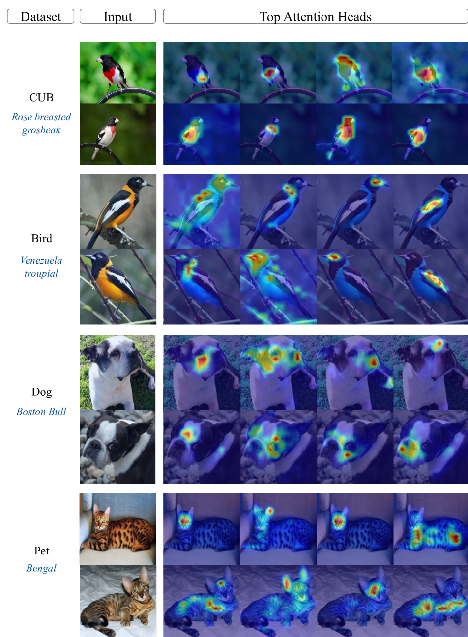
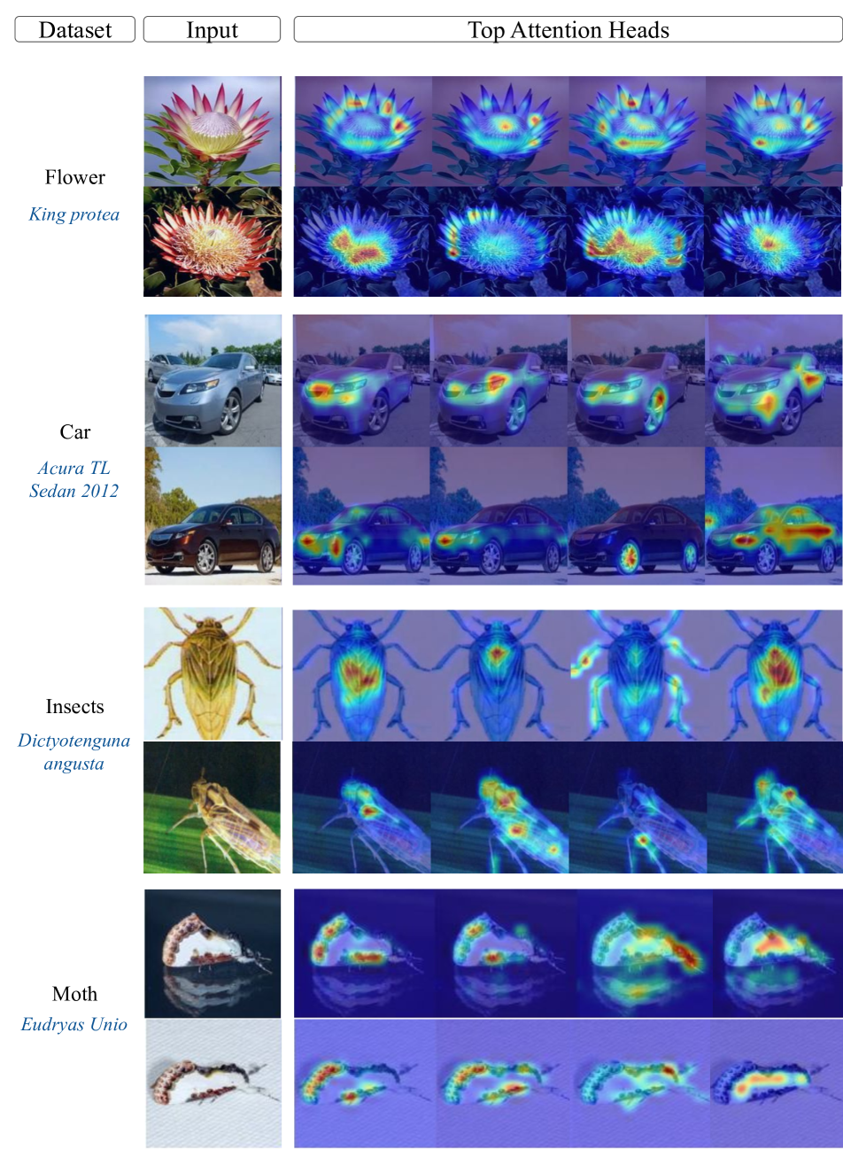
Figure 4: Visualization of Prompt-CAM on eight datasets. We show the top four attention maps (from left to right) per correctly classified test example triggered by the ground-truth classes. As top head indices per image may vary, traits may not align across rows.

4 Experiments

4.1 Experimental Setup

Dataset. We comprehensively evaluate the performance of Prompt-CAM on 13 diverse fine-grained image classification datasets across three domains: (1) animal-based: CUB-200-2011 (CUB) [43], Birds-525 (Bird) [32], Stanford Dogs (Dog) [15], Oxford Pet (Pet) [29], iNaturalist-2021-Moths (Moth) [41], Fish Vista (Fish) [23], Rare Species (RareS.) [40] and Insects-2 (Insects) [47]; (2) plant and fungi-based: iNaturalist-2021-Fungi (Fungi) [41], Oxford Flowers (Flower) [27] and Medicinal Leaf (MedLeaf) [35]; (3) object-based: Stanford Cars (Car) [16] and Food 101 (Food) [2]. We provide details about data processing and statistics in Suppl.

Model. We consider three pre-trained ViT backbones, DINO [4], DINOv2 [28], and BioCLIP [37] across different scales including ViT-B (the main one we use) and ViT-S. The backbones are kept completely frozen when applying Prompt-CAM. More details can be found in Suppl.

Baseline Methods. We compared Prompt-CAM with explainable methods like Grad-CAM [36], Layer-CAM [13] and Eigen-CAM [24] as well as with interpretable methods like ProtoPFormer [49], TesNet [45], ProtoConcepts [20] and INTR [30]. More details are in Suppl.

4.2 Experiment Results

Is Prompt-CAM faithful? For the faithfulness analysis, we apply Grad-CAM [36], Eigen-CAM [24], and Layer-CAM [13] to generate post-hoc saliency maps on the Linear Probing classifier as baselines. We then compare these with Prompt-CAM using the insertion and deletion metrics [31]. As shown in Table 1, Prompt-CAM yields significantly higher insertion scores and lower deletion scores, indicating a stronger focus on discriminative image traits and highlighting Prompt-CAM’s enhanced interpretability over standard post-hoc algorithms.

Table 1: Faithfulness evaluation based on insertion and deletion scores. A higher insertion score and a lower deletion score indicate better results. The results are obtained from the validation images of CUB using the DINO backbone.

	Insertion$\uparrow$	Deletion$\downarrow$
Grad-CAM	0.52	0.16
Layer-CAM	0.54	0.13
Eigen-CAM	0.42	0.33
Prompt-CAM	0.61	0.09

Prompt-CAM excels in trait identification (human assessment). Human assessment is conducted to evaluate trait identification quality for Prompt-CAM, TesNet [45], and ProtoConcepts [20]. Participants with no prior knowledge about the algorithms were instructed to compare the expert-identified traits (in text, such as orange belly) and the top heatmaps generated by each method. If an expert-identified trait is seen in the heatmaps, it is considered identified by the algorithm. On average, participants recognized $60.49\%$ of traits for Prompt-CAM, significantly outperforming TesNet and ProtoConcepts whose recognition rates are $39.14\%$ and $30.39$%, respectively. The results highlight Prompt-CAM’s superiority in emphasizing and conveying relevant traits effectively. More details are in Suppl.

Classification accuracy comparison. Building on the discussion in subsection 3.5, we observe that Prompt-CAM shows a slight accuracy drop compared to Linear Probing (see Table 2). However, the images misclassified by Prompt-CAM but correctly classified by Linear Probing align with our design philosophy: Prompt-CAM classifies images based on the presence of class-specific, localized traits and would fail if they are invisible. As illustrated in Figure 5, discriminative traits—such as the red breast of the Red-breasted Grosbeak—are barely visible in images misclassified by Prompt-CAM due to occlusion, unusual poses, or lighting conditions. Linear Probing correctly classifies them by leveraging global information such as body shapes and backgrounds. Please see more analysis in Suppl.

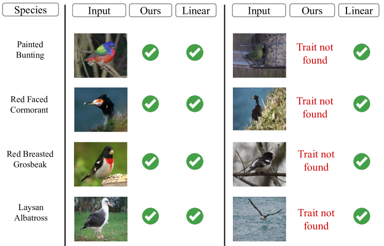
Figure 5: Images misclassified by Prompt-CAM but correctly classified by Linear Probing. Species-specific traits—such as the red breast of Red-breasted Grosbeak—are barely visible in misclassified images while Linear Probing uses global features such as body shapes, poses, and backgrounds for correct predictions.

Table 2: Accuracy (%) comparison using the DINO backbone.

	Bird	CUB	Dog	Pet
Linear Probing	98.1	78.6	82.4	92.4
Prompt-CAM	97.4	71.9	77.0	87.6

Comparison to interpretable models. We conduct a qualitative analysis to compare Prompt-CAM with other interpretable methods—ProtoPFormer, INTR, TesNet, and ProtoConcepts. Figure 6 shows the top-ranked attention maps or prototypes generated by each method. Prompt-CAM can capture a more extensive range of distinct, fine-grained traits, in contrast to other methods that often focus on a narrower or repetitive set of attributes (for example, ProtoConcepts in the first three ranks of the fifth row). This highlights Prompt-CAM’s ability to identify and localize different traits that collectively define a category’s identity.

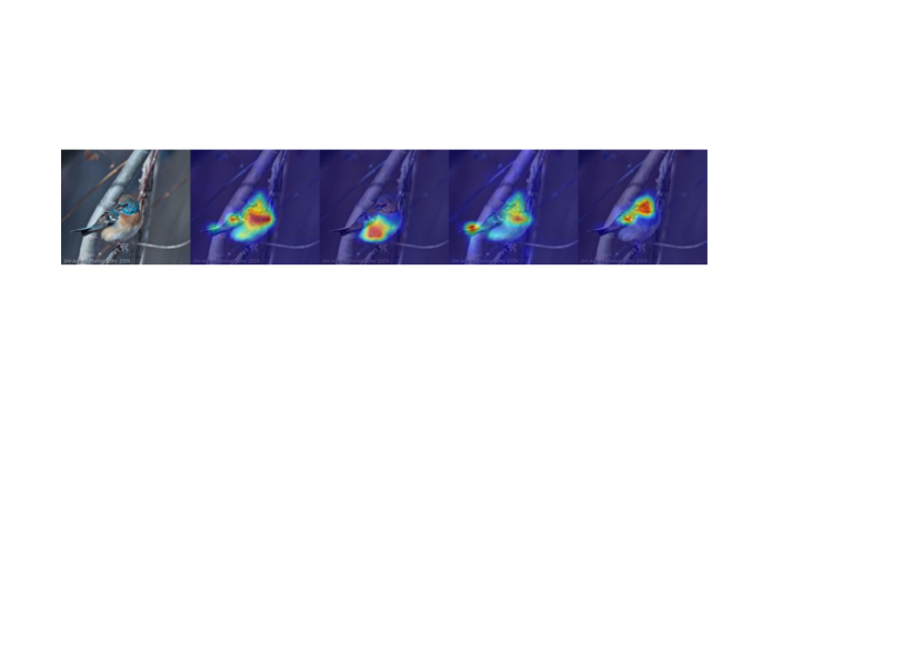
Figure 6: Comparison of interpretable models. Visual demonstration (heatmaps and bounding boxes) of the four most activated responses of attention heads (Prompt-CAM and INTR) or prototypes of each method on a Lazuli Bunting example image.

4.3 Further Analysis and Discussion

Prompt-CAM on different backbones. Figure 7 illustrates that Prompt-CAM is compatible with different ViT backbones. We show the top three attention maps generated by Prompt-CAM using different ViT backbones on an image of “Scott Oriole.” These maps highlight consistent identification of traits for species recognition, irrespective of the backbones. Please see the caption and Suppl. for details.

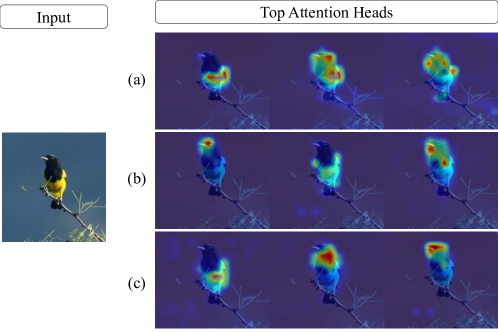
Figure 7: Prompt-CAM on different backbones. Here we show the top attention maps for Prompt-CAM on (a) DINO, (b) DINOv2, and (c) BioCLIP backbone. All three sets of attention heads point to consistent key traits of the species “Scott Oriole”—yellow belly, black head, and black chest.

Prompt-CAM on different datasets. Figure 4 presents the top four attention maps generated by Prompt-CAM across various datasets spanning diverse domains, including animals, plants, and objects. Prompt-CAM effectively captures the most important traits in each case to accurately identify species, demonstrating its remarkable generalizability and wide applicability.

Prompt-CAM can detect biologically meaningful traits. Figure 1 illustrates that Prompt-CAM can consistently identify traits from images of the same species to recognize it (e.g., breast color and wing pattern in the first and second columns of Figure 1.b for Baltimore Oriole). Another species like Bronzed Cowbird may see some of its traits from the images (e.g., head color and wing pattern in Figure 1.c) but not all of them (e.g., breast color), thus is unable to claim the images as Bronzed Cowbird. These results demonstrate Prompt-CAM’s ability to recognize species in a biologically meaningful way.

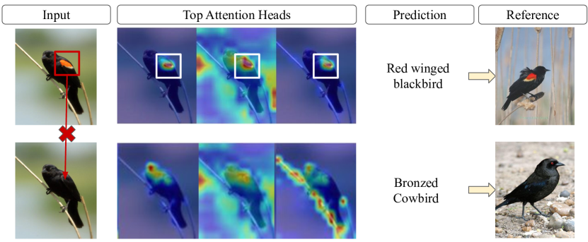
Figure 8: Trait manipulation. The top row shows attention maps for a correctly classified Red-winged Blackbird image. In the second row, the red spot on the bird’s wings was removed, and Prompt-CAM subsequently classified it as a Bronzed Cowbird, as depicted in the reference column.

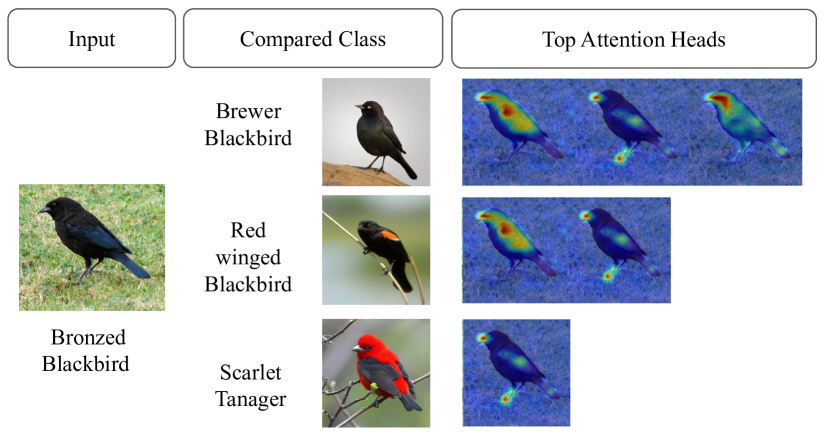
Figure 9: Focused Prompt-CAM (subsection 3.4) applied to pair-wise comparison. Given different references, Prompt-CAM looks at different (numbers of) traits to recognize the input image. For visually close species (Bronzed Blackbird vs. Brewer Blackbird), Prompt-CAM needs to look at the eye difference, which is not needed in differentiating visually dissimilar species.

Prompt-CAM can identify and interpret trait manipulation. We conduct a counterfactual-style analysis to investigate whether Prompt-CAM truly relies on the identified traits for making predictions. For instance, to correctly classify the Red-winged Blackbird, Prompt-CAM highlights the red wing patch (the first row of Figure 8), consistent with the field guide provided by the Cornell Lab of Ornithology. When we remove this red spot from the image to resemble a Bronzed Cowbird, Prompt-CAM no longer highlights the original position of the red patch. As such, it does not predict the image as a Red-winged Blackbird but a Bronzed Cowbird (the second row of Figure 8). This shows Prompt-CAM’s sensitivity to trait differences, showcasing its interpretability in fine-grained recognition.

Prompt-CAM uncovers subtle patterns in pair-wise comparison. Following the discussion in subsection 3.4, we illustrate Prompt-CAM’s capability to identify subtle differences between visually similar categories in Figure 9. From the bottom up, the compared classes become more visually similar to the true class, necessitating that Prompt-CAM identifies additional traits for recognition.

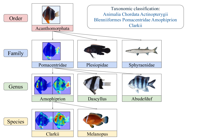
Figure 10: Prompt-CAM can detect taxonomically meaningful traits. Give an image of the species “Amophiprion Clarkii,” Prompt-CAM highlights the pelvic fin and double stripe to distinguish it from “Amophiprion Melanopus” at the species level. When it goes to the genus level, Prompt-CAM looks at the pattern in the body and tail to classify the image as the “Amophiprion” genus. As we go up, fishes at the family level become visually dissimilar. Prompt-CAM only needs to look at the tail and pelvic fin to classify the image as the “Pomacentridae” family.

Prompt-CAM can detect taxonomically meaningful traits. We train Prompt-CAM based on a hierarchical framework, considering four levels of taxonomic hierarchy: Order $\rightarrow$ Family $\rightarrow$ Genus $\rightarrow$ Species of Fish Dataset. In this setup, Prompt-CAM progressively shifts its focus from coarse-grained traits at the Family level to fine-grained traits at the Species level to distinguish categories (shown in Figure 10). This progression suggests Prompt-CAM’s potential to automatically identify and localize taxonomy keys to aid in biological and ecological research domains. We provide more details in Suppl.

5 Conclusion

We present Prompt Class Attention Map (Prompt-CAM), an effective interpretable method that leverages pre-trained ViTs to identify and localize traits for distinguishing among fine-grained categories. Prompt-CAM is easy to implement and train. Extensive experiments across domains such as animals, plants, and objects demonstrate Prompt-CAM’ superior performance and underscore the potential of repurposing standard models for interpretability.

Supplementary Material

The supplementary is organized as follows.

• Appendix A: Additional Related Work (cf. section 2 of the main paper)

• Appendix B: Details of Architecture Variant (cf. subsection 3.4 of the main paper)

• Appendix C: Dataset Details (cf. subsection 4.1 of the main paper)

• Appendix D: Inner Workings of Visualization (cf. subsection 3.3 of the main paper)

• Appendix E: Additional Experiment Settings (cf. subsection 4.1 of the main paper)

• Appendix F: Additional Experiment Results and Analysis (cf. subsection 4.2 of the main paper)

• Appendix G: More visualizations of different dataset (cf. Figure 4 of the main paper)

Appendix A Related Work

Pre-trained Vision Transformer. Vision Transformers (ViT) [9], pre-trained on massive amounts of data, has become indispensable to modern AI development. For example, ViTs pre-trained with millions of image-text pairs via a contrastive objective function (e.g., a CLIP-ViT model) show an unprecedented zero-shot capability, robustness to distribution shifts and serve as the encoders for various power generative models (e.g. Stable Diffusion [34] and LLaVA [18]). Domain-specific CLIP-based models like BioCLIP [37] and RemoteCLIP [17], trained on millions of specialized image-text pairs, outperform general-purpose CLIP models within their respective domains. Moreover, ViTs trained with self-supervised objectives on extensive sets of well-curated images, such as DINO and DINOv2 [4, 28], effectively capture fine-grained localization features that explicitly reveal object and part boundaries. We employ DINO, DINOv2, and BioCLIP as our backbone models in light of our focus on fine-grained analysis.

Prompting Vision Transformer. Traditional approaches to adapt pre-trained transformers—full fine-tuning and linear probing—face challenges: the former is computationally intensive and prone to overfitting, while the latter struggles with task-specific adaptation [21, 22]. Prompting, first popularized in natural language processing (NLP), addressed such challenges by prepending task-specific instructions to input text, enabling large language models like GPT-3 to perform zero-shot and few-shot learning effectively [3].

Recently, prompting has been introduced in vision transformers (ViTs) to enable efficient adaptation while leveraging the vast capabilities of pre-trained ViTs. Visual Prompt Tuning (VPT) [12] introduces learnable embedding vectors, either in the first transformer layer or across layers, which serve as “prompts” while keeping the backbone frozen. This offers a lightweight and scalable alternative to full fine-tuning, achieving competitive performance on a diverse range of tasks while preserving the pre-trained features.

Explainable methods. Understanding the decision-making process of neural networks has gained significant traction, particularly in tasks where model transparency is critical. Explainable methods (XAI) focus on post-hoc analysis to provide insights into pre-trained models without altering their structure. Methods like Class Activation Mapping (CAM) [50] and Gradient-weighted CAM (Grad-CAM) [36] visualize class-specific contributions by projecting gradients onto feature maps. Subsequent improvements, such as Score-CAM [44] and Eigen-CAM [24], incorporate global feature contributions or principal component analysis to generate more detailed explanations. Despite these advancements, many XAI methods produce coarse, low-resolution heatmaps, which can be imprecise and fail to fully capture the model’s decision-making process.

Interpretable methods. In contrast, interpretable methods provide a direct understanding of predictions by aligning intermediate representations with human-interpretable concepts. Early approaches such as ProtoPNet [6] utilized “learnable prototypes” to represent class-specific features, enabling visual comparison between input features and prototypical examples. Extensions like ProtoConcepts [20], ProtoPFormer [49], and TesNet [45] have refined this approach, integrating prototypes into transformer-based architectures to achieve higher accuracy and interoperability. More recent advancements leverage transformer architectures to enable interpretable decision-making. For example, Concept Transformers utilize query-based encoder-decoder designs to discover meaningful concepts [33], while methods like INTR [30] employ competing query mechanisms to elucidate how the model arrives at specific predictions. While these approaches offer fine-grained interpretability, they require substantial modifications to the backbone, leading to increased training complexity and longer computational times for new datasets.

Prompt-CAM aims to overcome the shortcomings of both approaches. The special prediction mechanism encourages explainable, class-specific attention that is aligned well with model predictions. Simultaneously, we leverage pre-trained ViTs by simply modifying the usage of task-specific prompts without altering the backbone architecture.

Appendix B Details of Architecture Variant

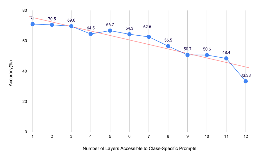
Figure 11: Accuracy versus the number of layers (from last layer to first) attended by class-specific prompts. As the number of attended layers increases in class-specific prompts, accuracy decreases, highlighting the importance of class-agnostic prompts. The more class-agnostic prompts a model has, the better trait localization and higher accuracy are achieved.

In this section, we explore variations of Prompt-CAM by experimenting with the placement of class-specific prompts within the vision transformer (ViT) architecture. While Prompt-CAM-Shallow introduces class-specific prompts in the first layer and Prompt-CAM-Deep applies them in the final layer, we also investigate injecting these prompts at various intermediate layers. Specifically, we control the layer depth at which class-specific prompts are added and analyze their impact on feature interpolation.

In Prompt-CAM-Shallow, class-specific prompts are introduced at the first layer ($i=1$), allowing them to interact with patch features across all transformer layers (i.e., $\bm{E}_{i}$, $i=0,\cdots,N-1$) without using class-agnostic prompts. As we increase the layer index $i$ where class-specific prompts are added, the number of layers class-specific prompts interact decreases. At the same time, the number of preceding class-agnostic prompts increases, which interacts with the preceding $(i-1)$ layers (mentioned in subsection 3.2).

In Figure 12, we demonstrate the relationship between the number of layers accessible to class-specific prompts and their ability to localize fine-grained traits effectively. The visualization provides a clear pattern: as the prompts attend only to the last layer (first row) (same as Prompt-CAM-Deep), their focus is highly localized on discriminative traits, such as the red patch on the wings of the “Red-Winged Blackbird.” This precise focus enables the model to excel in fine-grained trait analysis.

As we move downward through the rows, class-specific prompts attending to increasingly more layers (from top to bottom), the attention maps become progressively more diffused. For instance, in the middle rows (e.g., rows 6–8), the attention begins to cover broader regions of the object rather than the trait of interest. This diffusion correlates with a drop in accuracy, as seen in the accuracy plot, Figure 11.

In the bottom rows (e.g., rows 10–11), the attention becomes scattered and unfocused, covering irrelevant regions. This fails to correctly classify the object. The accuracy plot confirms this trend: as the class-specific prompts attend to more layers, accuracy steadily decreases.

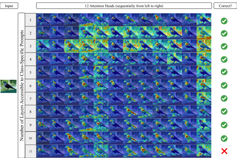
Figure 12: Visualization of attention maps for different configurations of Prompt-CAM. For a random image of the “Red-Winged Blackbird” species, twelve attention heads of the last layer of Prompt-CAM on the DINO backbone are shown for the ground truth class prompt. The first row shows class-specific prompts attending to only the last layer (as Prompt-CAM-Deep), resulting in highly localized attention on fine-grained traits, such as the red patch on the wings of the “Red-Winged Blackbird.” As these prompts attend to increasingly more layers (progressing down the rows), the attention becomes more diffuse, covering broader regions of the object and eventually leading to a loss of focus on relevant traits.

Appendix C Dataset Details

Table 3: Dataset statistics (Animals).

	Animals
	Bird	CUB	Dog	Pet	Insects	Fish	Moth	RareS.
# Train Images	84,635	5,994	12,000	3,680	52,603	35,328	5,000	9,584
# Test Images	2,625	5,795	8,580	3,669	22,619	7,556	1,000	2,399
# Labels	525	200	120	37	102	414	100	400

Table 4: Dataset statistics (Plants & Fungi and Objects).

	Plants & Fungi			Objects
	Flower	MedLeaf	Fungi	Car	Food
# Train Images	2,040	1,455	12,250	8,144	75,750
# Test Images	6,149	380	2,450	8,041	25,250
# Labels	102	30	245	196	101

We comprehensively evaluate the performance of Prompt-CAM on a diverse set of benchmark datasets curated for fine-grained image classification across multiple domains. The evaluation includes animal-based datasets such as CUB-200-2011 (CUB) [43], Birds-525 (Bird) [32], Stanford Dogs (Dog) [15], Oxford Pet (Pet) [29], iNaturalist-2021-Moths (Moth) [41], Fish Vista (Fish) [23], Rare Species (RareS.) [40] and Insects-2 (Insects) [47]. Additionally, we assess performance on plant and fungi-based datasets, including iNaturalist-2021-Fungi (Fungi) [41], Oxford Flowers (Flower) [27] and Medicinal Leaf (MedLeaf) [35]. Finally, object-based datasets, such as Stanford Cars (Car) [16] and Food 101 (Food) [2], are also included to ensure comprehensive coverage across various fine-grained classification tasks. For the Moth and Fungi dataset, we extract species belonging to Noctuidae Family from taxonomic class Animalia Arthropoda Insecta Lepidoptera Noctuidae and species belonging to Agaricomycetes Class from taxonomic path Fungi$\rightarrow$ Basidiomycota, respectively, from the iNaturalist-2021 dataset. For hierarchical classification and trait localization, we use taxonomical information from the Fish and iNaturalist-2021 dataset. We provide dataset statistics in Table 3 and Table 4.

Appendix D Inner Workings of Visualization

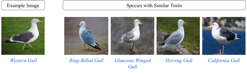
Figure 13: Example Image of a “Western Gull” and its closest bird species, highlighting overlapping traits. Correctly classifying the “Western Gull” requires attention to multiple subtle traits, as it shares many traits with similar species. This highlights the need to examine a broader range of attributes for accurate classification.

Which traits are more discriminative? As discussed in subsection 3.3, certain categories within the CUB dataset exhibit distinctive traits that are highly discriminative. For instance, in the case of the “Red-winged Blackbird,” the defining features are its red-spotted black wings. Similarly, the “Ruby-throated Hummingbird” is characterized by its ruby-colored throat and sharp, long beak. However, some species require consideration of multiple traits to distinguish them from others. For example, correctly classifying a “Western Gull” demands attention to several subtle traits (Figure 13), as it shares many features with other species. This observation raises a key question: can we automatically identify and rank the most important traits for a given image of a species?

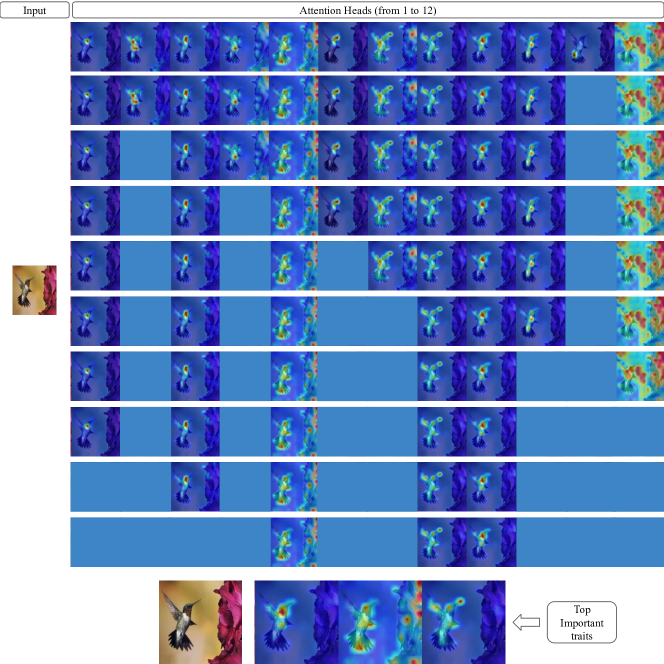
Figure 14: Greedy approach to identify and rank important traits for species classification. For the species “Ruby Throated Hummingbird”, we progressively blur attention heads (from top to bottom), retaining only the traits necessary for correct classification, using the Prompt-CAM on the DINO backbone. The blurred attention heads are shown in solid blue color.

To address this, we propose a greedy algorithm that progressively “blurs” traits in a correctly classified image until its decision changes. This process reveals the traits that are both necessary and sufficient for the correct prediction.

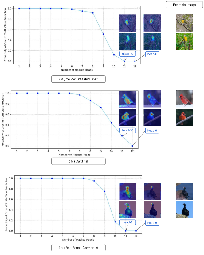
Figure 15: Visualization of ground truth class probability vs. the number of masked heads at the species level in Prompt-CAM. The left plots show how the probability of the ground truth class changes for all correctly classified images in a species, as heads are progressively masked in the greedy approach discussed in Appendix D. For class (a) “Yellow Breasted Chat,” the probability drops significantly after masking eight heads, indicating that the last four heads are critical. The top two heads, head-6 and head-10, focus on the yellow breast and lower belly. For class (b) “Cardinal,” the top 2 heads, head-9 and head-10, attend to the black pattern on the face and the red belly. In class (c) “Red Faced Cormorant,” the critical heads, head-6 and head-9, emphasize the red head and the neck’s shape. These results highlight the interpretability of Prompt-CAM in identifying essential traits for each species.

Greedy approach for identifying discriminative traits: Suppose class $c$ is the true class and the image is correctly classified. In the first greedy step, for each attention head, $r=1,\cdots,R$ (R attention heads), we iteratively replace the attention vector ${\bm{\alpha}}^{c,r}_{N-1}$, with a uniform distribution:

$${\bm{\alpha}}^{c,r}_{N-1}\leftarrow\frac{1}{M}\mathbf{1},$$

where $\mathbf{1}\in\mathbb{R}^{M}$ is a vector of all ones, and $M$ is the number of patches. This replacement effectively assigns equal importance to all patches in the attention weights, thereby “blurring” the $r$-th head’s contribution to class $c$. After this modification, we recalculate the score $s[c]$ in Equation 1.

For each iteration, we select the attention head $r^{*}$ that, when blurred, results in the highest probability for the correct class $c$. This head $r^{*}$ is then added to $B_{a}$ (set of blurred attention heads), as the blurred head with the highest $s[c]$ is the least important and contributes the least discriminative information for class $c$. We repeat this process, iteratively blurring additional heads and updating $B_{a}$, until blurring any remaining head not in $B_{a}$ changes the model’s prediction. In Figure 14, for an image of “Ruby Throated Hummingbird” we show this greedy approach, by progressively blurring out the attention heads in each step, retaining only necessary traits.

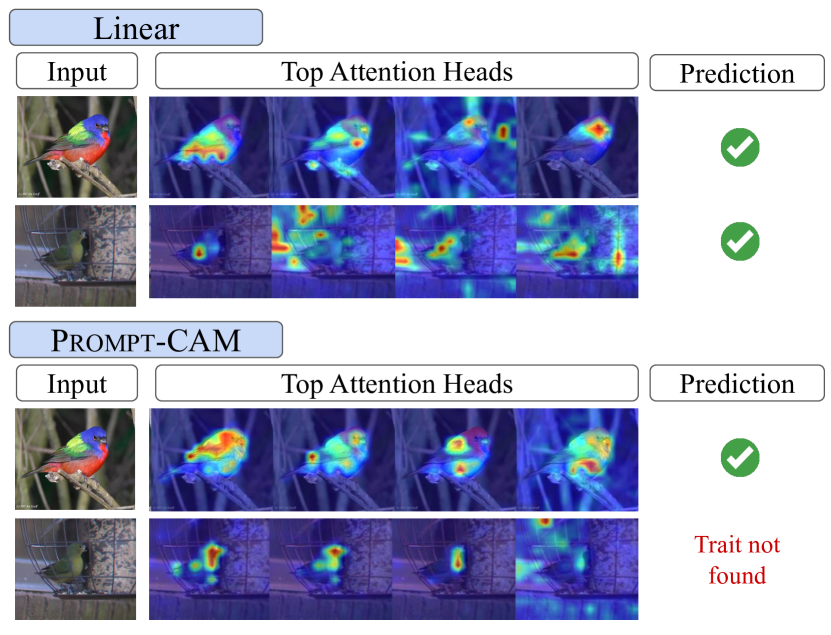
Figure 16: Comparison of top attention heads for Prompt-CAM and Linear probing on two images of the species “Painted Bunting.” For the correctly classified image by both, Prompt-CAM focuses on meaningful traits such as the blue head, wings, tail, and red lower belly, while Linear probing produces noisy and less diverse heatmaps. For the other image, Linear probing relies on global memorized attributes for correct classification, whereas Prompt-CAM attempts to identify object-specific traits, resulting in an interpretable misclassification due to poor visibility of key features.

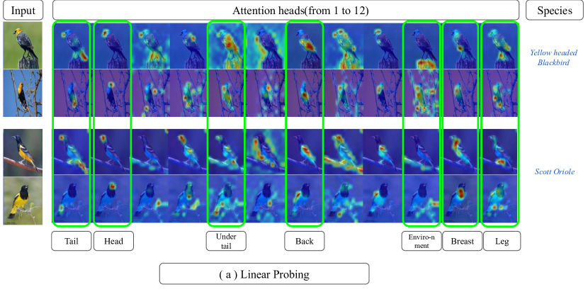
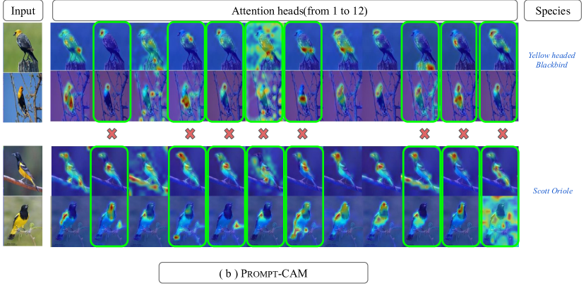
Figure 17: Comparison of attention heatmaps for Linear Probing and Prompt-CAM. On random images of “Yellow Headed Blackbird” and “Scott Oriole” from the CUB dataset, in (a), Linear Probing consistently focuses on similar body parts (e.g., tail, head, under-tail, wings) across all species, showing limited adaptability to traits specific to each class. In contrast, (b) Prompt-CAM (using pretrained DINO) dynamically adapts its attention to focus on distinct and meaningful traits required for class-specific identification. For instance, Prompt-CAM highlights traits such as the yellow head and breast for “Yellow Headed Blackbird” and the wing pattern for “Scott Oriole”.

Attention head vs species. In addition to image-level analysis, we conduct a species-level investigation to determine whether certain attention heads consistently focus on important traits across all images of a species. Using the greedy approach discussed in the above paragraph, we analyze each correctly classified image of a species $c$ to iteratively select the attention head $r^{*}$ that minimally impacts the probability of the correct class $c$. We then examine how the probability $s[c]$ changes as attention heads are progressively blurred or masked for all images of a species. This analysis, visualized in Figure 15, demonstrates that for most species in the CUB dataset, approximately four attention heads capture traits critical for class prediction. In the Figure 15, we highlight the top-2 attention heads for example images from various species. The results reveal that these heads consistently focus on important, distinctive traits for their respective species. For instance, in the case of the “Cardinal”, head-9 focuses on the black stripe near the beak, while head-10 attends to the red breast color—traits essential for identifying the species. Similarly, for “Yellow-breasted Chat” and “Red-faced Cormorant”, attention heads consistently highlight relevant features across their respective species. These findings emphasize the robustness of our approach in identifying class-specific discriminative traits and the flexibility of choosing any number of ranked important traits per species.

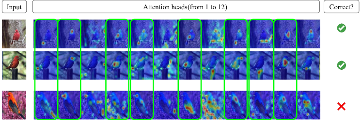
Figure 18: Attention heatmaps of cls-token for Linear Probing on misclassified images. For some random images of “Scarlet Tanager” from the CUB dataset, Linear Probing highlights the same body parts across images, failing to provide meaningful insights into misclassifications.

Appendix E Additional Experiment Settings

E.1 Implementation Details

Dataset-specific settings. For DINO backbone, the learning rate varied across datasets within the set $\{0.01,0.1,0.125\}$, selected based on dataset-specific characteristics. For Bird and MedLeaf, training was conducted for 30 epochs. For all other datasets, training was conducted for 100 epochs. For DINOv2 backbone, the learning rate varied across datasets within the set of $\{0.005,0.01\}$, selected based on dataset-specific characteristics. For Insect, CUB, and Bird, training was conducted for 130 epochs. For all other datasets, training was conducted for 100 epochs. For DINOv2 backbone, the learning rate varied across datasets within the set of $\{0.05,0.01\}$, selected based on dataset-specific characteristics. For all datasets, training was conducted for 100 epochs. A batch size of 64 was used for all datasets and all backbones.

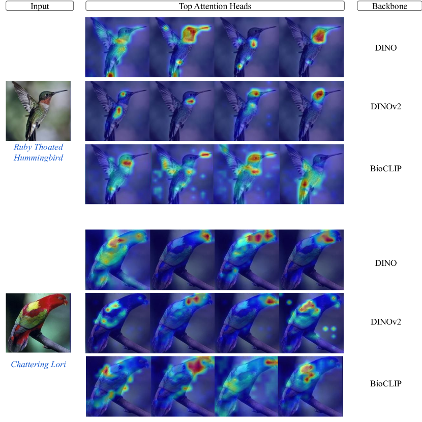
Figure 19: Visualization of top attention heads of Prompt-CAM for DINO, DINOv2 and BioCLIP backbones. For random correctly classified images from “Ruby Throated Hummingbird” and “Chattering Lori” species from Bird Dataset, top-4 attention heads (from left to right) are shown. Prompt-CAM can identify and locate meaningful important traits for species regardless of pre-trained visual backbone used.

Optimization settings. Stochastic Gradient Descent (SGD) optimizer with a momentum of 0.9. Weight Decay 0.0 was used for all datasets for DINO, 0.001 for the rest. A cosine learning rate scheduler was applied, with a warmup period of 10 epochs and cross-entropy loss was used.

E.2 Baseline Methods

We used XAI methods Grad-CAM, Score-CAM, and Eigen-CAM to compare Prompt-CAM performance with them on a quantitative scale. For qualitative comparison, we compare with a variety of interpretable methods, ProtoPFormer, TesNet, INTR, and ProtoPConcepts shown in Figure 6.

Appendix F Additional Experiment Results

Model performance analysis. As discussed in subsection 3.3, we analyze misclassified examples by Prompt-CAM, illustrated in Figure 5. We attribute the slight decline in accuracy of Prompt-CAM to its approach of forcing prompts to focus on the object itself and its traits, rather than relying on surrounding context for classification. In Figure 16, we compare the heatmaps of two images of the species “Painted Bunting”. The first image, $I_{c}$, is correctly classified by both Prompt-CAM and Linear probing, while the second image, $I_{m}$, is correctly classified by Linear probing but misclassified by Prompt-CAM. The image $I_{m}$ presents additional challenges: it is poorly lit, further from the camera, and depicts a less common gender of the species in the CUB dataset.

For $I_{c}$, the top heatmaps from Linear probing appear noisy and less diverse compared to Prompt-CAM. In contrast, Prompt-CAM exhibits a more meaningful focus, with its top attention heads targeting the blue head, part of the wings, the tail, and the red lower belly—traits characteristic of the species.

In the case of $I_{m}$, although Linear probing predicts the image correctly, its top attention heads fail to focus on consistent traits. Instead, they appear to rely on global features memorized from the training dataset, resulting in a lack of meaningful interpretation. On the other hand, Prompt-CAM, despite misclassifying $I_{m}$, focuses its attention on traits within the object itself. The heatmaps reveal that Prompt-CAM attempts to identify relevant features, but the lack of visible traits in the image leads to an interpretable misclassification.

In Figure 17, the comparison between Linear Probing and Prompt-CAM in the attention heatmaps reveals a fundamental difference in their classification and trait identification approach. As shown in the heatmaps, Linear Probing uniformly distributes its attention across similar body parts, such as the tail, head, and wings, irrespective of the species being analyzed. This behavior indicates that Linear Probing relies on global patterns that may not be specific to any particular class. In contrast, for each species, Prompt-CAM focuses on specific traits important for differentiating one class from another. For example, in the case of the “Yellow Headed Blackbird,” Prompt-CAM emphasizes the yellow head and breast, traits unique to the species. Similarly, for the “Scott Oriole,” the yellow breast and wing patterns are prominently highlighted. By prioritizing traits essential for species identification, Prompt-CAM provides a more robust and meaningful framework for understanding model decisions.

Furthermore, in Figure 18, we present attention heatmaps for random images of the “Scarlet Tanager” species from the CUB dataset, generated using Linear Probing. Linear Probing consistently assigns attention to the same body parts (e.g., wings, head) across images, without providing meaningful insights into the reasons for misclassification. In contrast, Prompt-CAM (as shown in Figure 8 and Figure 16) provides a more interpretable explanation for misclassifications. When Prompt-CAM misclassifies an image, it is evident that the misclassification occurs due to the absence of the necessary trait in the image, demonstrating its focus on biologically relevant and class-specific traits.

This analysis underscores Prompt-CAM prioritizes interpretability, ensuring that its classifications are based on meaningful and consistent traits, even at the cost of a slight accuracy decline.

Human assessment of trait identification settings. In subsection 4.2, we discussed how we measured robustness of Prompt-CAM with assessment from human observers. To evaluate the effectiveness of trait identification, in the human assessment, we compared Prompt-CAM, TesNet [45], and ProtoConcepts [20]. A total of 35 participants with no prior knowledge of the models participated in the study. Participants were presented with a set of top attention heatmaps (Prompt-CAM and INTR) or prototypes generated by each method and image-specific class attributes found in CUB dataset. Then they were asked to identify and check the traits they perceived as being highlighted in the heatmaps. The traits were taken from the CUB dataset, where image-specific traits are present. We used four random correctly classified images by every method, from four species “Cardinal”, “Painted Bunting”, “Rose Breasted Grosbeak” and “Red faced Cormorant” to generate attention heatmaps/prototypes.

The assessment revealed that participants recognized $60.49\%$ of the traits highlighted by Prompt-CAM, significantly outperforming TesNet and ProtoConcepts, which achieved recognition rates of $39.14\%$ and $30.39\%$, respectively. These findings demonstrate Prompt-CAM’s superior ability to emphasize and communicate relevant traits effectively to human observers.

Prompt-CAM on different backbones. We implement Prompt-CAM on multiple pre-trained vision transformers, including DINO, DINOv2, and Bioclip. In Table 5, we present the accuracy of Prompt-CAM across various datasets using different backbones: DINO (ViT-Base/16), DINOv2 (ViT-Base/14), and Bioclip (ViT-Base/16). For each model, we visualize the top-4 attention heads on the Bird Dataset in Figure 19. Notably, Bioclip achieves higher accuracy on biology-specific datasets, which we attribute to its pre-training on an extensive biology-focused dataset, enabling it to develop a highly specialized feature space for these species. Additionally, we also evaluate Prompt-CAM on other DINO variations, ViT-Base/8 (accuracy: $73.9\%$) and ViT-Small/8 (accuracy: $68.3\%$) on the CUB dataset, achieving comparable performance and interpretability to DINO ViT-Base/16 (accuracy: $71.9\%$) (shown in Figure 20). This demonstrates Prompt-CAM’s robustness, flexibility, and ease of implementation across various pre-trained vision transformer backbones and datasets.

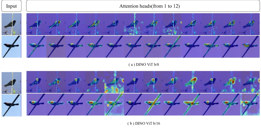
Figure 20: Visualization of attention heads for pre-trained DINO backbone variants. For correctly classified images of “Red winged blackbird”, with Prompt-CAM, both DINO ViT b/16 and DINO ViT b/8 backbones can capture traits for classification.

Table 5: Accuracy of Prompt-CAM on different backbones. To show the flexibility and robustness, the accuracy of Prompt-CAM on multiple datasets is shown implemented on pre-trained vision transformers, DINO, DINOv2 and BioCLIP.

		Bird	CUB	Dog	Pet	Insects-2	Flowers	Med.Leaf	Rare Species
Ours	DINO	97.4	71.9	77.0	87.6	64.7	86.4	99.1	60.8
	DINOv2	98.2	73.8	80.0	91.7	70.6	91.9	99.6	62.2
	BioCLIP	98.6	84.0	73.1	87.2	71.8	95.7	99.6	67.1

Taxonomical hierarchy trait discovery settings. In hierarchical taxonomic classification in biology, each level in the taxonomy leverages specific traits for classification. As we move down the taxonomic hierarchy, the traits become increasingly fine-grained. Motivated by this observation, we trained and visualized traits in a hierarchical taxonomic manner using the Fish Vista dataset.

We first constructed a taxonomic tree spanning from Kingdom to Species. For the Family level, we aggregated all images belonging to the diverse species under their respective Family and performed classification to assign images to the appropriate Family. As shown in Figure 10, even coarse traits, such as the tail and pelvic fin, were sufficient to classify an image of the species “Amphiprion Melanopus” to its’ correct Family (attribute information found in Fish Dataset).

At the Genus level, we create a new dataset for each Family by grouping all images from the children nodes of each Family and dividing them into classes by their respective Genus. For instance, within the “Pomacentridae” Family, finer traits like stripe patterns, pelvic fins, and tails became necessary to classify its’ Genus accurately for the same example image. Finally, at the Species level, all images from the children nodes of each Genus were used to create a new dataset and were divided into classes. For the example image in Figure 10, distinguishing between these two species now requires looking at subtle differences such as the pelvic fin structure and the number of white stripes on the body for the same image from the “Amphiprion Melanopus” species. This hierarchical approach offers an exciting framework to discover traits in a manner that is both evolutionary and biologically meaningful, enabling a deeper understanding of trait importance across taxonomic levels.

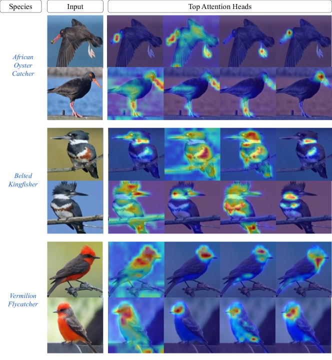
Figure 21: Visualization of Prompt-CAM on Bird Dataset. We show the top four attention maps (from left to right) per correctly classified test example, triggered by the ground-truth classes. As top head indices per image may vary, traits may not align across columns.

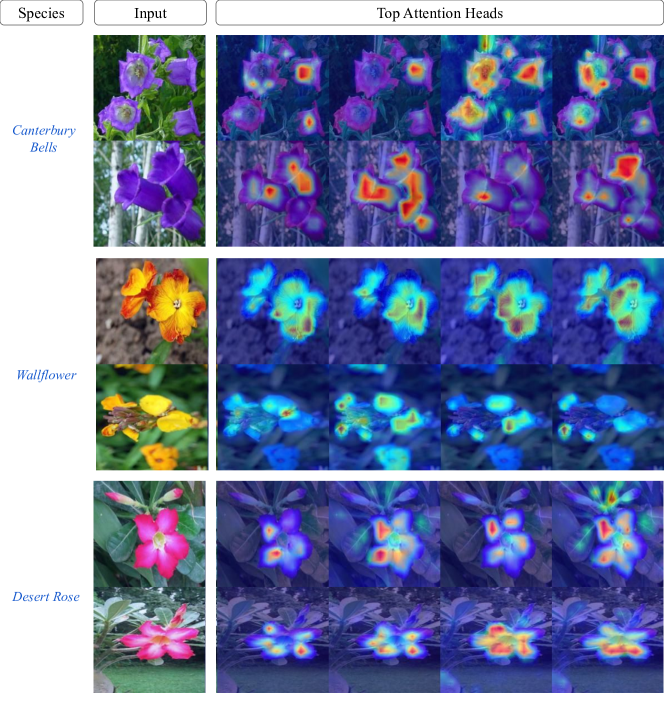
Figure 22: Visualization of Prompt-CAM on Flower Dataset. We show the top four attention maps (from left to right) per correctly classified test example, triggered by the ground-truth classes. As top head indices per image may vary, traits may not align across columns.

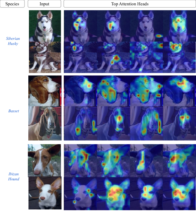
Figure 23: Visualization of Prompt-CAM on Dog Dataset. We show the top four attention maps (from left to right) per correctly classified test example, triggered by the ground-truth classes. As top head indices per image may vary, traits may not align across columns.

Appendix G More Visualizations

In this section, we show the top-4 attention maps triggered by ground truth classes for correctly predicted classes, for some datasets mentioned Appendix C, following the same format of Figure 4. Each attention head of Prompt-CAM for each dataset successfully identifies different and important attributes of each class of every dataset. For some datasets, if the images of a class are simple enough, we might need less than four heads to predict.

References

- Abnar and Zuidema [2020] Samira Abnar and Willem Zuidema. Quantifying attention flow in transformers. arXiv preprint arXiv:2005.00928, 2020.
- Bossard et al. [2014] Lukas Bossard, Matthieu Guillaumin, and Luc Van Gool. Food-101–mining discriminative components with random forests. In Computer vision–ECCV 2014: 13th European conference, zurich, Switzerland, September 6-12, 2014, proceedings, part VI 13, pages 446–461. Springer, 2014.
- Brown et al. [2020] Tom B. Brown, Benjamin Mann, Nick Ryder, Melanie Subbiah, Jared Kaplan, Prafulla Dhariwal, Arvind Neelakantan, Pranav Shyam, Girish Sastry, Amanda Askell, Sandhini Agarwal, Ariel Herbert-Voss, Gretchen Krueger, Tom Henighan, Rewon Child, Aditya Ramesh, Daniel M. Ziegler, Jeffrey Wu, Clemens Winter, Christopher Hesse, Mark Chen, Eric Sigler, Mateusz Litwin, Scott Gray, Benjamin Chess, Jack Clark, Christopher Berner, Sam McCandlish, Alec Radford, Ilya Sutskever, and Dario Amodei. Language models are few-shot learners. In Proceedings of the 34th International Conference on Neural Information Processing Systems, 2020.
- Caron et al. [2021] Mathilde Caron, Hugo Touvron, Ishan Misra, Hervé Jégou, Julien Mairal, Piotr Bojanowski, and Armand Joulin. Emerging properties in self-supervised vision transformers. In Proceedings of the International Conference on Computer Vision (ICCV), 2021.
- Chefer et al. [2021] Hila Chefer, Shir Gur, and Lior Wolf. Transformer interpretability beyond attention visualization. In Proceedings of the IEEE/CVF conference on computer vision and pattern recognition, pages 782–791, 2021.
- Chen et al. [2019] Chaofan Chen, Oscar Li, Daniel Tao, Alina Barnett, Cynthia Rudin, and Jonathan K Su. This looks like that: deep learning for interpretable image recognition. Advances in neural information processing systems, 32, 2019.
- Darcet et al. [2024] Timothée Darcet, Maxime Oquab, Julien Mairal, and Piotr Bojanowski. Vision transformers need registers. In ICLR, 2024.
- Deng et al. [2024] Yihe Deng, Yu Yang, Baharan Mirzasoleiman, and Quanquan Gu. Robust learning with progressive data expansion against spurious correlation. Advances in neural information processing systems, 36, 2024.
- Dosovitskiy et al. [2021] Alexey Dosovitskiy, Lucas Beyer, Alexander Kolesnikov, Dirk Weissenborn, Xiaohua Zhai, Thomas Unterthiner, Mostafa Dehghani, Matthias Minderer, Georg Heigold, Sylvain Gelly, Jakob Uszkoreit, and Neil Houlsby. An image is worth 16x16 words: Transformers for image recognition at scale. In International Conference on Learning Representations, 2021.
- He et al. [2022] Ju He, Jie-Neng Chen, Shuai Liu, Adam Kortylewski, Cheng Yang, Yutong Bai, and Changhu Wang. Transfg: A transformer architecture for fine-grained recognition. In Proceedings of the AAAI conference on artificial intelligence, pages 852–860, 2022.
- Jackson and Somers [1991] Darneisha A Jackson and Keith M Somers. The spectre of ‘spurious’ correlations. Oecologia, 86:147–151, 1991.
- Jia et al. [2022] Menglin Jia, Luming Tang, Bor-Chun Chen, Claire Cardie, Serge Belongie, Bharath Hariharan, and Ser-Nam Lim. Visual prompt tuning. In European Conference on Computer Vision, pages 709–727. Springer, 2022.
- Jiang et al. [2021] Peng-Tao Jiang, Chang-Bin Zhang, Qibin Hou, Ming-Ming Cheng, and Yunchao Wei. Layercam: Exploring hierarchical class activation maps for localization. IEEE Transactions on Image Processing, 30:5875–5888, 2021.
- Kashefi et al. [2023] Rojina Kashefi, Leili Barekatain, Mohammad Sabokrou, and Fatemeh Aghaeipoor. Explainability of vision transformers: A comprehensive review and new perspectives. arXiv preprint arXiv:2311.06786, 2023.
- Khosla et al. [2011] Aditya Khosla, Nityananda Jayadevaprakash, Bangpeng Yao, and Fei-Fei Li. Novel dataset for fine-grained image categorization: Stanford dogs. In Proceedings CVPR workshop on fine-grained visual categorization (FGVC), 2011.
- Krause et al. [2013] Jonathan Krause, Michael Stark, Jia Deng, and Li Fei-Fei. 3d object representations for fine-grained categorization. In Proceedings of the IEEE international conference on computer vision workshops, pages 554–561, 2013.
- Liu et al. [2024a] Fan Liu, Delong Chen, Zhangqingyun Guan, Xiaocong Zhou, Jiale Zhu, Qiaolin Ye, Liyong Fu, and Jun Zhou. Remoteclip: A vision language foundation model for remote sensing. IEEE Transactions on Geoscience and Remote Sensing, 2024a.
- Liu et al. [2024b] Haotian Liu, Chunyuan Li, Qingyang Wu, and Yong Jae Lee. Visual instruction tuning. In Advances in neural information processing systems, 2024b.
- Liu et al. [2021] Shilong Liu, Lei Zhang, Xiao Yang, Hang Su, and Jun Zhu. Query2label: A simple transformer way to multi-label classification. arXiv preprint arXiv:2107.10834, 2021.
- Ma et al. [2024] Chiyu Ma, Brandon Zhao, Chaofan Chen, and Cynthia Rudin. This looks like those: Illuminating prototypical concepts using multiple visualizations. Advances in Neural Information Processing Systems, 36, 2024.
- Mai et al. [2024a] Zheda Mai, Arpita Chowdhury, Ping Zhang, Cheng-Hao Tu, Hong-You Chen, Vardaan Pahuja, Tanya Berger-Wolf, Song Gao, Charles Stewart, Yu Su, et al. Fine-tuning is fine, if calibrated. In The Thirty-eighth Annual Conference on Neural Information Processing Systems, 2024a.
- Mai et al. [2024b] Zheda Mai, Ping Zhang, Cheng-Hao Tu, Hong-You Chen, Li Zhang, and Wei-Lun Chao. Lessons learned from a unifying empirical study of parameter-efficient transfer learning (petl) in visual recognition. arXiv preprint arXiv:2409.16434, 2024b.
- Mehrab et al. [2024] Kazi Sajeed Mehrab, M Maruf, Arka Daw, Harish Babu Manogaran, Abhilash Neog, Mridul Khurana, Bahadir Altintas, Yasin Bakis, Elizabeth G Campolongo, Matthew J Thompson, et al. Fish-vista: A multi-purpose dataset for understanding & identification of traits from images. arXiv preprint arXiv:2407.08027, 2024.
- Muhammad and Yeasin [2020] Mohammed Bany Muhammad and Mohammed Yeasin. Eigen-cam: Class activation map using principal components. In 2020 international joint conference on neural networks (IJCNN), pages 1–7. IEEE, 2020.
- Nauta et al. [2021] Meike Nauta, Ron Van Bree, and Christin Seifert. Neural prototype trees for interpretable fine-grained image recognition. In Proceedings of the IEEE/CVF conference on computer vision and pattern recognition, pages 14933–14943, 2021.
- Ng et al. [2023] Kam Woh Ng, Xiatian Zhu, Yi-Zhe Song, and Tao Xiang. Dreamcreature: Crafting photorealistic virtual creatures from imagination. arXiv preprint arXiv:2311.15477, 2023.
- Nilsback and Zisserman [2008] Maria-Elena Nilsback and Andrew Zisserman. Automated flower classification over a large number of classes. In 2008 Sixth Indian conference on computer vision, graphics & image processing, pages 722–729. IEEE, 2008.
- Oquab et al. [2023] Maxime Oquab, Timothée Darcet, Theo Moutakanni, Huy V. Vo, Marc Szafraniec, Vasil Khalidov, Pierre Fernandez, Daniel Haziza, Francisco Massa, Alaaeldin El-Nouby, Russell Howes, Po-Yao Huang, Hu Xu, Vasu Sharma, Shang-Wen Li, Wojciech Galuba, Mike Rabbat, Mido Assran, Nicolas Ballas, Gabriel Synnaeve, Ishan Misra, Herve Jegou, Julien Mairal, Patrick Labatut, Armand Joulin, and Piotr Bojanowski. Dinov2: Learning robust visual features without supervision, 2023.
- Parkhi et al. [2012] Omkar M Parkhi, Andrea Vedaldi, Andrew Zisserman, and CV Jawahar. Cats and dogs. In 2012 IEEE conference on computer vision and pattern recognition, pages 3498–3505, 2012.
- Paul et al. [2024] Dipanjyoti Paul, Arpita Chowdhury, Xinqi Xiong, Feng-Ju Chang, David Carlyn, Samuel Stevens, Kaiya Provost, Anuj Karpatne, Bryan Carstens, Daniel Rubenstein, Charles Stewart, Tanya Berger-Wolf, Yu Su, and Wei-Lun Chao. A simple interpretable transformer for fine-grained image classification and analysis. In International Conference on Learning Representations, 2024.
- Petsiuk et al. [1806] V Petsiuk, A Das, and K Saenko. Rise: Randomized input sampling for explanation of black-box models. arxiv 2018. arXiv preprint arXiv:1806.07421, 1806.
- Piosenka [2023] Gerald Piosenka. Birds 525 species - image classification. 2023.
- Rigotti et al. [2021] Mattia Rigotti, Christoph Miksovic, Ioana Giurgiu, Thomas Gschwind, and Paolo Scotton. Attention-based interpretability with concept transformers. In International conference on learning representations, 2021.
- Rombach et al. [2022] Robin Rombach, Andreas Blattmann, Dominik Lorenz, Patrick Esser, and Björn Ommer. High-resolution image synthesis with latent diffusion models. In Proceedings of the IEEE/CVF conference on computer vision and pattern recognition, pages 10684–10695, 2022.
- S and J [2020] Roopashree S and Anitha J. Medicinal Leaf Dataset, 2020. Mendeley Data, V1.
- Selvaraju et al. [2017] Ramprasaath R Selvaraju, Michael Cogswell, Abhishek Das, Ramakrishna Vedantam, Devi Parikh, and Dhruv Batra. Grad-cam: Visual explanations from deep networks via gradient-based localization. In Proceedings of the IEEE international conference on computer vision, pages 618–626, 2017.
- Stevens et al. [2024] Samuel Stevens, Jiaman Wu, Matthew J Thompson, Elizabeth G Campolongo, Chan Hee Song, David Edward Carlyn, Li Dong, Wasila M Dahdul, Charles Stewart, Tanya Berger-Wolf, et al. Bioclip: A vision foundation model for the tree of life. In Proceedings of the IEEE/CVF Conference on Computer Vision and Pattern Recognition, pages 19412–19424, 2024.
- Tang et al. [2023a] Luming Tang, Menglin Jia, Qianqian Wang, Cheng Perng Phoo, and Bharath Hariharan. Emergent correspondence from image diffusion. Advances in Neural Information Processing Systems, 36:1363–1389, 2023a.
- Tang et al. [2023b] Zhenchao Tang, Hualin Yang, and Calvin Yu-Chian Chen. Weakly supervised posture mining for fine-grained classification. In Proceedings of the IEEE/CVF Conference on Computer Vision and Pattern Recognition, pages 23735–23744, 2023b.
- Team [2023] Imageomics Team. Rare Species Dataset, 2023. Dataset with 400 classes of rare species images and descriptions sourced from the Encyclopedia of Life and the IUCN Red List.
- Van Horn et al. [2021] Grant Van Horn, Elijah Cole, Sara Beery, Kimberly Wilber, Serge Belongie, and Oisin Mac Aodha. Benchmarking representation learning for natural world image collections. In Proceedings of the IEEE/CVF conference on computer vision and pattern recognition, pages 12884–12893, 2021.
- Vaswani et al. [2017] Ashish Vaswani, Noam Shazeer, Niki Parmar, Jakob Uszkoreit, Llion Jones, Aidan N. Gomez, Łukasz Kaiser, and Illia Polosukhin. Attention is all you need. In Proceedings of the 31st International Conference on Neural Information Processing Systems, page 6000–6010, 2017.
- Wah et al. [2011] Catherine Wah, Steve Branson, Peter Welinder, Pietro Perona, and Serge Belongie. The caltech-ucsd birds-200-2011 dataset. 2011.
- Wang et al. [2020] Haofan Wang, Zifan Wang, Mengnan Du, Fan Yang, Zijian Zhang, Sirui Ding, Piotr Mardziel, and Xia Hu. Score-cam: Score-weighted visual explanations for convolutional neural networks. In Proceedings of the IEEE/CVF conference on computer vision and pattern recognition workshops, pages 24–25, 2020.
- Wang et al. [2021] Jiaqi Wang, Huafeng Liu, Xinyue Wang, and Liping Jing. Interpretable image recognition by constructing transparent embedding space. In Proceedings of the IEEE/CVF international conference on computer vision, pages 895–904, 2021.
- Wang et al. [2023] Shijie Wang, Jianlong Chang, Haojie Li, Zhihui Wang, Wanli Ouyang, and Qi Tian. Open-set fine-grained retrieval via prompting vision-language evaluator. In Proceedings of the IEEE/CVF Conference on Computer Vision and Pattern Recognition, pages 19381–19391, 2023.
- Wu et al. [2019] Xiaoping Wu, Chi Zhan, Yu-Kun Lai, Ming-Ming Cheng, and Jufeng Yang. Ip102: A large-scale benchmark dataset for insect pest recognition. In Proceedings of the IEEE/CVF conference on computer vision and pattern recognition, pages 8787–8796, 2019.
- Xu et al. [2022] Lian Xu, Wanli Ouyang, Mohammed Bennamoun, Farid Boussaid, and Dan Xu. Multi-class token transformer for weakly supervised semantic segmentation. In Proceedings of the IEEE/CVF conference on computer vision and pattern recognition, pages 4310–4319, 2022.
- Xue et al. [2022] Mengqi Xue, Qihan Huang, Haofei Zhang, Lechao Cheng, Jie Song, Minghui Wu, and Mingli Song. Protopformer: Concentrating on prototypical parts in vision transformers for interpretable image recognition. arXiv preprint arXiv:2208.10431, 2022.
- Zhou et al. [2016] Bolei Zhou, Aditya Khosla, Agata Lapedriza, Aude Oliva, and Antonio Torralba. Learning deep features for discriminative localization. In Proceedings of the IEEE conference on computer vision and pattern recognition, pages 2921–2929, 2016.
- Zhu et al. [2022] Haowei Zhu, Wenjing Ke, Dong Li, Ji Liu, Lu Tian, and Yi Shan. Dual cross-attention learning for fine-grained visual categorization and object re-identification. In Proceedings of the IEEE/CVF conference on computer vision and pattern recognition, pages 4692–4702, 2022.