MINDS: Motor Imitation Assessment Network for Distinguishing Children with Autism

Computerized Assessment of Motor Imitation for Distinguishing Autism in Video (CAMI-2DNet)

Abstract

Motor imitation impairments are commonly reported in individuals with autism spectrum conditions (ASCs), suggesting that motor imitation could be used as a phenotype for addressing autism heterogeneity. Traditional methods for assessing motor imitation are subjective and labor-intensive, and require extensive human training. Modern Computerized Assessment of Motor Imitation (CAMI) methods, such as CAMI-3D for motion capture data and CAMI-2D for video data, are less subjective. However, they rely on labor-intensive data normalization and cleaning techniques, and human annotations for algorithm training. To address these challenges, we propose CAMI-2DNet, a scalable and interpretable deep learning-based approach to motor imitation assessment in video data, which eliminates the need for data normalization, cleaning and annotation. CAMI-2DNet uses an encoder-decoder architecture to map a video to a motion encoding that is disentangled from nuisance factors such as body shape and camera views. To learn a disentangled representation, we employ synthetic data generated by motion retargeting of virtual characters through the reshuffling of motion, body shape, and camera views, as well as real participant data. To automatically assess how well an individual imitates an actor, we compute a similarity score between their motion encodings, and use it to discriminate individuals with ASCs from neurotypical (NT) individuals. Our comparative analysis demonstrates that CAMI-2DNet has a strong correlation with human scores while outperforming CAMI-2D in discriminating ASC vs NT children. Moreover, CAMI-2DNet performs comparably to CAMI-3D while offering greater practicality by operating directly on video data and without the need for ad-hoc data normalization and human annotations.

Autism Spectrum Conditions, Behavior Analysis, Motor Imitation Assessment, Motion Analysis in Video Data, Disentangled Motion Representation Learning.

1 Introduction

Imitating the actions of others plays a fundamental role in the formation of social bonds and the acquisition of essential skills, particularly during early development and in human interactions [1]. However, individuals with autism spectrum conditions (ASCs) often exhibit atypical imitation patterns, reflecting core social and communicative challenges [2]. Assessing these imitation patterns is essential for understanding the unique developmental needs of individuals with ASCs and plays a critical role in early diagnosis and intervention.

Human Observation Coding (HOC) has long been the standard method for assessing imitation, providing a detailed and nuanced examination of individuals’ motor imitation skills through direct observation by trained human coders. However, while HOC has provided valuable insights into the specific challenges and variations in imitation that are indicative of ASC-related impairments, HOC has several limitations. First and foremost, it is inherently subjective, relying on the interpretation and judgment of human observers, which can introduce biases and inconsistencies in the assessment process. Second, the HOC process is labor-intensive, requiring significant time, effort, and trained personnel to analyze and code behaviors accurately. Its manual nature makes it impractical limiting the ability to scale imitation and other motor assessments to clinical and home settings.

With the increasing prevalence of ASCs and the growing demand for early and accurate assessments, there is a need for automated and objective assessment tools that address the challenges associated with HOC in evaluating motor imitation. The development of tools that are effective and widely applicable offers several potential advantages, including efficiency, objectivity, and scalability. However, the development of such tools faces several challenges including (i) the diverse range and complex nature of human actions involved in imitation, (ii) the trade-off between sensitivity and specificity in recognizing atypical imitation patterns, and (iii) the need to ensure the adaptability of the tool across diverse settings.

Several automated methods have been proposed for addressing these challenges [3, 4, 5, 6, 7, 8, 9]. Among them, motion-capture-based methods have proven to be effective as they rely on precise 3-dimensional (3D) motion data which enables a more accurate analysis of the subtleties in human movement. One example is the Computerized Assessment of Motor Imitation (CAMI) method. CAMI-3D [10] takes 3D motion data acquired from Kinect Xbox cameras as input and uses a combination of Dynamic Time Warping (DTW) [11] and linear regression to produce a similarity score that takes into account variations in both motion trajectories and timing discrepancies. The findings of this method on autism diagnosis were encouraging [10], demonstrating high test-retest reliability and surpassing the performance of HOC in effectively discriminating children with ASCs from neurotypical (NT) children as well as from children with Attention-Deficit/Hyperactivity Disorder (ADHD), a highly prevalent condition that is both a differential diagnosis of ASC as well as a frequent co-occurring diagnosis [12].

However, despite its promising results, CAMI-3D has several limitations. First, its scalability is hindered by its dependence on Kinect or other 3D cameras, which may impede its applicability in settings where such specialized hardware is not readily available (e.g., homes and clinics). Second, it requires cumbersome frame-by-frame manual cleaning of a subject’s skeleton to obtain motion coordinates, which can potentially take hours, especially if part of the body is consistently outside the point-cloud, rotated incorrectly, or occluded. Third, it uses hand-crafted normalization techniques to handle natural variations in body structure (e.g., height, limb length) and slight differences in camera angles. While these techniques may be effective within the specific context of a study, they could lack adaptability to the wide range of anatomical and pose variations encountered in real-world scenarios. Furthermore, the HOC annotations are required during training, thus requiring continued human input for new action sequences.

To address the dependence on costly 3D motion capture devices and make motion analysis more accessible and scalable, one can leverage recent advances in 2D pose estimation techniques in computer vision [13, 14, 15], which allow for accurate detection and tracking of skeletal joints in video data captured using readily available 2D cameras. These advances motivated the development of CAMI-2D [16], which uses an off-the-shelf pose estimation network, OpenPose [13], to extract 2D joints from video data, DTW to compare these 2D trajectories, and linear regression to produce an imitation score, as in CAMI-3D. However, CAMI-2D inherits CAMI-3D limitations such as the need for hand-crafted normalization and HOC annotations. Moreover, 2D joint locations are more heavily affected by camera viewpoint due to perspective projection and occlusions. Therefore, comparing 2D trajectories can be misleading as these trajectories are affected by nuisance factors such as variations in body shape and camera viewpoint.

Recent advances in deep learning offer a more robust and efficient approach to comparing human movements in video data [17, 18]. The key idea is to use a neural network to map the video to an abstract, compressed motion representation that captures the essence of the movements. This is achieved by using large-scale video data or pose sequences to learn disentangled representations, i.e., motion representations that are invariant to nuisance factors such as body shape and camera viewpoint. For example, [19] proposes a novel approach for decomposing motion data into dynamic and static representations. Originally developed for motion retargeting, this technique utilizes an encoder-decoder network to separate motion data into skeleton-independent dynamic features and skeleton-dependent static features. The model in[20] further decomposes a pose sequence into individual body parts, generating representations for each part separately. This results in motion representations that are suitable for measuring the similarity between different motions of each part. The network is trained with a motion variation loss, enhancing its ability to distinguish even subtly different motions. However, these methods are not directly applicable for distinguishing an individual with ASC as they need very large training datasets to be able to distinguish fine-grained differences in motion, e.g., when an individual is trying to imitate precise movements.

In this work, we propose CAMI-2DNet, a novel deep learning-based method to assess motor imitation for distinguishing individuals with ASC in video data. CAMI-2DNet utilizes an encoder-decoder architecture that learns distinct motion representations disentangled from nuisance factors such as skeletal shape and camera views. Disentangling motion representation from these nuisance factors is crucial for ensuring that the model accurately captures the essence of the movements themselves, without being influenced by irrelevant variations. For example, people with different body types may perform the same movement in slightly different ways due to variations in limb length or skeletal structure. If the model does not disentangle these factors, it might incorrectly attribute these differences to the quality of the imitation, rather than as natural variations due to the person’s physical characteristics. Similarly, variations in camera angles or distances could make identical motions look different. By isolating the motion characteristics from these factors, CAMI-2DNet can consistently evaluate the quality of motor imitation, regardless of an individual’s height, body shape, or whether the video was recorded from a different angle, thereby eliminating the need for labor-intensive tasks like manual frame-by-frame data cleaning and ad-hoc normalization, which are needed in methods like CAMI-3D and CAMI-2D.

To effectively learn these disentangled representations, we employ large-scale synthetic data generated by motion retargeting of virtual characters through the reshuffling of motion, body, and camera views, along with participant data from individuals with ASCs and neurotypical individuals. CAMI-2DNet automatically assesses a person’s imitation performance by computing a similarity score between motion encodings, which can then be used for autism diagnosis. CAMI-2DNet addresses critical limitations of existing manual methods such as HOC and automated systems such as CAMI-3D and CAMI-2D by providing a quick, reliable, and easy-to-use tool for assessing imitation. Therefore, CAMI-2DNet has the potential to enable the use of more frequent, accessible, and detailed assessments, facilitating earlier and more accurate diagnoses, and more personalized treatment planning.

Specifically, the contributions of this paper are as follows:

• A deep-learning-based approach to motor imitation assessment. CAMI-2DNet uses an encoder-decoder architecture trained on (a) large-scale synthetic data generated through motion retargeting and (b) participant data from individuals with ASCs as well as neurotypical individuals to effectively disentangle complex motion, skeletal structures, and camera viewpoint from a video, providing a more robust assessment of motor imitation.

• Objective and quantitative assessment. CAMI-2DNet provides a quantitative motion imitation score obtained by comparing the motion representations of the individual and an actor, leading to an objective metric that reduces the subjectivity and variability of human-coded methods such as HOC.

• Interpretability through localized scores. By segmenting the motion representation into different body parts and movement types, CAMI-2DNet offers localized imitation scores, which not only improves the interpretability of the results but also has the potential to enable tailored interventions based on the specific imitation deficits identified in individuals with ASCs.

• Scalability and practicality. Unlike CAMI-3D, which relies on specialized 3D cameras and HOC annotations for training, CAMI-2DNet operates directly on standard video input and does not depend on HOC annotations. This capability significantly enhances the practicality and scalability of our method, making it suitable for use in varied settings including clinics and home environments without the need for specialized hardware.

• Empirical validation. The comparative analysis conducted between CAMI-2DNet and current assessment methods (HOC, CAMI-3D, and CAMI-2D) demonstrates that CAMI-2DNet correlates strongly with HOC scores and shows superior performance in classifying children into diagnostic groups. Moreover, CAMI-2DNet matches the performance of CAMI-3D while offering significant advantages in terms of ease of use and independence from specialized equipment or the need for HOC annotations. These findings validate CAMI-2DNet as a highly effective and practical tool for assessing motor imitation for distinguishing children with autism in video captured using standard off-the-shelf 2D cameras.

2 Overview of CAMI-2DNet

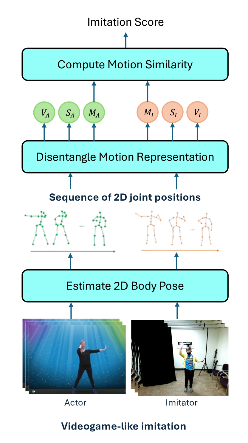
(a) Overview

 

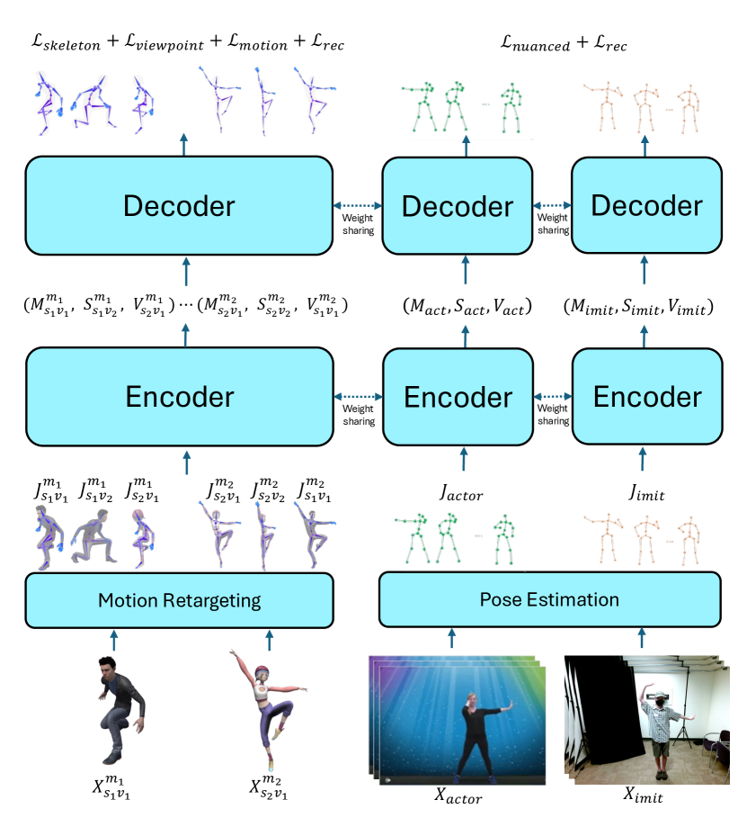
(b) Training Process

Figure 1: The overall architecture of CAMI-2DNet, including (a) an overview of the method and (b) the training process – (a) The overview of the method illustrates how CAMI-2DNet computes the imitation score. Given input videos of both an actor performing a target action and an individual imitating the action, a pose estimation network extracts sequences of 2D joint positions from the videos. These pose sequences are then encoded into disentangled motion, shape, and viewpoint representations. Only the motion representations ($M_{a}$ for the actor and $M_{i}$ for the individual) are used for comparison. The motion encodings are optimized and temporally aligned using Dynamic Time Warping (DTW), and the cosine similarity between the motion encodings is computed to produce the imitation score. (b) In the training process, the model learns disentangled motion, shape, and viewpoint representations using both synthetic and participant data from individuals with ASCs as well as neurotypical individuals. The synthetic data undergoes motion retargeting, where the same motion is performed by virtual characters with different shapes and from various viewpoints. For the participant data, pose estimation is applied to extract pose sequences from video recordings. These pose sequences are then processed by the encoder, which disentangles the interactions between motion ($M$), skeletal structures ($S$), and camera viewpoints ($V$). The decoder reconstructs the original pose sequences from these encodings to ensure the accurate learning of disentangled representations. Training on synthetic data is guided by losses for disentangle motion ($\mathcal{L}_{\text{motion}}$), shape ($\mathcal{L}_{\text{shape}}$), and viewpoint ($\mathcal{L}_{\text{viewpoint}}$), along with the reconstruction loss ($\mathcal{L}_{\text{rec}}$). For the participant data, the model is trained using both the nuanced motion loss ($\mathcal{L}_{\text{nuanced}}$) and the reconstruction loss ($\mathcal{L}_{\text{rec}}$).

In this section, we summarize our CAMI-2DNet method for distinguishing individuals with autism in video. Given a video of an actor performing a sequence of movements and a video of a person imitating the movements, the goal is to produce a score that quantifies how closely the person’s movements match those of the actor. This matching imitation score is then used to help discriminate an individual with ASCs from NT.

2.1 Stages of CAMI-2DNet

An overview of CAMI-2DNet is illustrated in Figure 1(a). CAMI-2DNet comprises three main stages: estimating body pose, disentangling motion representation, and computing the imitation score. Here is a summary of each stage, with further details provided in the corresponding sections.

• Estimate 2D Body Pose: Extract sequence of 2D body joints (e.g., elbows, knees) from each video, converting visual data to 2D trajectories suitable for motion analysis.

• Disentangle Motion Representation: Map the sequence of 2D body joints to a learnable motion representation that is disentangled from nuisance factors such as variations in body shape or camera viewpoint.

• Compute Motion Imitation Score: Use the disentangled motion representation to compute a score that quantifies how well a person imitates the movements of the actor.

These stages allow CAMI-2DNet to yield a more accurate and robust motor imitation assessment by disentangling the dynamics of motion and eliminating distortions caused by irrelevant variables such as body shape and camera viewpoint.

2.2 Estimating 2D Body Pose

The first step in CAMI-2DNet is to extract the 2D coordinates of the human body joints (e.g., elbows, knees, shoulders) in each video frame, a.k.a. 2D pose estimation. Given a video $\mathbf{X}\in\mathbb{R}^{T\times H\times W\times 3}$, where $T$ represents the number of frames and ($H$, $W$) denotes the height and width of each frame, a pose estimation model predicts the 2D coordinates of key body joints, which we represent as $\mathbf{J}\in\mathbb{R}^{T\times J\times 2}$, where $J$ is the number of body joints. These joint positions form a time series that tracks the subject’s body movements throughout the video, providing suitable data for understanding their motion in subsequent stages of motor imitation assessment.

In this work we employ a Vision Transformer-based pose estimation model, EViTPose [15], due to its ability to capture long-range dependencies between body parts while maintaining computational efficiency. This allows the model to generate accurate joint positions even in complex scenarios, such as when the subject is partially occluded or in varying postures.

To further enhance the specificity and interpretability of motor imitation assessments, we isolate different regions of the body to localize the motor imitation assessments and provide detailed insights into which specific areas may be contributing to any observed differences in motor imitation. Thus, we divide the overall pose sequence $\mathbf{J}$ into $S$ segments, each one corresponding to a specific body part (e.g., arms, legs, torso). We denote the joint trajectories for segment $\mathcal{S}$ by $\mathbf{J}_{\mathcal{S}}$, where $\mathcal{S}$ is the set of joint indices for that body part. For more details, please refer to Appendix 8.

2.3 Learning Disentangled Representations

While pose estimation provides raw data about the joint trajectories, motion imitation assessment based on comparing such trajectories can be misleading. This is because raw trajectories are affected by natural variations in body shape (e.g., height, limb length) or differences in camera angles and distances. These factors, referred to as nuisance factors, can distort the motion analysis, making it difficult to accurately evaluate how well a subject is imitating a target action.

For instance, consider a scenario where two people are performing the same action, such as raising an arm. One person might have a longer arm or a different posture due to natural skeletal differences. Thus, comparing the pose sequences could incorrectly suggest that the two people’s motions are fundamentally different when, in fact, the movement patterns are identical. Similarly, camera angles or distance variations can cause identical movements to appear different. For example, a movement recorded from a side view might look different from the same movement recorded from a front view. As discussed in the introduction, some prior approaches, such as CAMI-3D [10], attempt to address these nuisance factors using hand-crafted normalization techniques. CAMI-3D, for instance, adjusts joint coordinates based on estimated body proportions or reorients poses to account for changes in the camera angle. While these hand-crafted techniques, which rely on pre-set rules, may be effective within a controlled environment, they often struggle to generalize to the wide range of anatomical and positional variations encountered in real-world scenarios, leading to potential inaccuracies. Therefore, CAMI-2DNet goes beyond pose estimation by learning disentangled representations of motion, shape, and viewpoint. The goal is to extract a pure motion encoding that remains unaffected by body shape or viewpoint variations, allowing for a fair and accurate comparison of the actor’s and an individual’s movements as discussed in detail in Section 3.

2.4 Computing Motion Similarity

After disentangling the motion from skeletal and viewpoint variations, the next step in CAMI-2DNet is computing an imitation score that quantifies how closely an individual’s movements mimic those of the actor. CAMI-2DNet focuses solely on the motion encodings of both the actor and the person, ignoring any irrelevant factors related to body shape or camera angle. By comparing these disentangled motion representations, CAMI-2DNet provides a robust, objective measure of motor imitation performance. This score serves as a reliable indicator of how well a person imitates an action, enabling the system to discriminate typical motor imitation abilities from potential signs of impairment, such as those associated with ASCs [2]. The details of how we compute the motion imitation score are discussed in Section 4.

3 Learning a Disentangled Motion Representation

As discussed in the previous section, simply relying on raw pose sequences for motor imitation assessment is insufficient due to the entanglement of motion with irrelevant factors like body shape and camera viewpoint. To address these challenges, a key component of CAMI-2DNet is to automatically learn a motion representation from the raw pose sequences that is disentangled from these nuisance factors. In this section, we discuss how CAMI-2DNet achieves this disentanglement. First, we describe the encoder-decoder model architecture that processes pose sequences to produce disentangled motion, shape, and viewpoint encodings. Next, we discuss the role of training data, specifically motion retargeting and the integration of synthetic and participant data. Finally, we outline the training objectives that guide the model in learning robust and disentangled representations. The overall training process is illustrated in Figure 1(b), which provides a visual summary of how CAMI-2DNet leverages both synthetic and real data to achieve effective disentanglement of motion, shape, and viewpoint components.

3.1 Model Architecture

To effectively learn a representation disentangled from nuisance factors, we employ an encoder-decoder architecture. The encoder compresses the input pose sequences into latent representations that focus on different action components, while the decoder reconstructs the original pose sequence to validate the quality of the learned representation.

3.1.1 Encoding

The encoder is designed to isolate the core characteristics of motion so that the learned representation accurately reflects the subject’s motor abilities, free from distortions caused by skeletal structure and camera perspectives. The encoding process is formally defined as:

$$(\mathbf{M},\mathbf{S},\mathbf{V})=f_{\text{enc}}(\mathbf{J};\theta_{\text{enc}}),$$ (1)

where $f_{\text{enc}}$ is the encoding network, parameterized by weights $\theta_{\text{enc}}$, which transforms the raw pose sequence $\mathbf{J}$ into three disentangled components: (i) $\mathbf{M}$ is a motion representation that captures the essence of the subject’s movement, (ii) $\mathbf{S}$ is a shape representation that models the body structure of the subject, which can vary across individuals, and (iii) $\mathbf{V}$ is a viewpoint representation that accounts for the camera perspective from which the movement is captured.

By disentangling these components, the encoder allows CAMI-2DNet to focus solely on the core aspects of the motion $\mathbf{M}$, independent of irrelevant factors like body structure $\mathbf{S}$ or camera viewpoint $\mathbf{V}$. This is crucial for enabling accurate motion comparisons across subjects and environments.

3.1.2 Decoding

The decoder plays a vital role in ensuring that the learned latent representation not only captures the essential characteristics of the motion but also retains sufficient information for accurate reconstruction of the original pose sequence. The decoder’s objective is to reconstruct the pose sequence $\hat{\mathbf{J}}$ from the disentangled representations, $\mathbf{M}$ (motion), $\mathbf{S}$ (shape), and $\mathbf{V}$ (viewpoint). This reconstruction ensures that the latent space adequately represents all the necessary details to model the original movement accurately. Formally, the decoding process is defined as:

$$\hat{\mathbf{J}}=f_{\text{dec}}(\mathbf{M},\mathbf{S},\mathbf{V};\theta_{\text{dec}}),$$ (2)

where $f_{\text{dec}}$ is the decoding network, parameterized by weights $\theta_{\text{dec}}$, which maps the disentagled components $\mathbf{M},\mathbf{S},$ and $\mathbf{V}$ to a reconstructed pose sequence $\hat{\mathbf{J}}$ that should match the original pose sequence $\mathbf{J}$ as closely as possible. Please refer to Appendix 7 for further details about the architecture.

3.2 Training Data

3.2.1 Motion Retargeting

Directly learning disentangled representations from real-world data is inherently challenging due to the absence of explicit information about the underlying motion, body shape, or camera viewpoint. In natural scenarios, the variations in motion are often entangled with differences in body shapes (e.g., height, limb length) and camera perspectives (e.g., angle, distance), making it difficult to isolate the core movement characteristics from irrelevant factors.

This is where motion retargeting becomes essential. Motion retargeting allows us to synthetically generate training data by systematically reshuffling motion, body shape, and camera viewpoint. More specifically, by having the same motion performed by different virtual characters with varying body shapes and by capturing the movements from multiple camera angles, we can create a diverse set of training samples that retain the same core motion dynamics but exhibit variation in body shape and viewpoint configurations.

We leverage the Synthetic Actors and Real Actions Dataset [21], a synthetic dataset generated via motion retargeting. In this dataset, virtual characters from a set $\mathcal{B}$ perform motions from a set $\mathcal{M}$, and these motions are observed from different viewpoints in a set $\mathcal{V}$. Each training sample includes pairs of virtual characters ${s_{1},s_{2}}\subseteq\mathcal{B}$ performing a triplet of motions ${m_{1},m_{2},m_{3}}\subseteq\mathcal{M}$, captured from two distinct viewpoints ${v_{1},v_{2}}\subseteq\mathcal{V}$. The motions $m_{1}$ and $m_{2}$ are variations within the same motion class – such as a low jump and a high jump – while $m_{3}$ is a distinctly different motion, such as sitting. By reshuffling these components, we ensure that the model learns robust, disentangled motion representations that are invariant to skeletal and viewpoint differences, ultimately leading to more accurate and fair motion comparisons.

3.2.2 Integrating Synthetic and Real Participant Data

While synthetic data is essential for learning disentangled representations, it introduces a domain gap: synthetic motions are generic and do not fully reflect the specific types of motions we target in motor imitation assessment for distinguishing ASCs. To address this gap, we adopt a mixed training process that combines synthetic and real participant data. Synthetic data lays the foundation for learning robust motion representations by disentangling motion from skeletal and viewpoint variations, while the participant data refines the model’s ability to adapt to the target motion types and captures nuanced differences present in practical settings. This integration ensures that the model benefits from the controlled variability of large-scale synthetic data while simultaneously adapting to the complexity and subtleties of real-world scenarios.

3.3 Training Objectives

During training, we employ a combination of loss functions tailored to both synthetic and participant data. These loss functions are crucial in guiding the model to effectively separate the core motion from irrelevant factors such as body shape and camera viewpoint, while also capturing the nuanced variations in motor imitation tasks.

For the synthetic data, the model is trained with losses that enforce the disentanglement of motion, shape, and viewpoint, in addition to the reconstruction loss. In contrast, the participant data training utilizes the reconstruction loss alongside a nuanced motion loss, which helps the model capture the subtleties of the motor imitation task.

3.3.1 Disentanglement Losses

Here, we describe the disentanglement loss functions, beginning with a common triplet loss formulation that is applied across all action components.

Triplet Loss: The triplet loss is designed to ensure that encodings of the same type (motion, shape, or viewpoint) are closer to each other than encodings of different types. The triplet consists of an anchor, a positive example (similar to the anchor), and a negative example (dissimilar to the anchor). The objective of the triplet loss is to minimize the distance between the anchor and the positive example while maximizing the distance between the anchor and the negative example, encouraging separation between distinct factors. Formally, the triplet loss for an anchor encoding $\mathbf{E}_{\text{A}}$ with its corresponding positive and negative example encodings $\mathbf{E}_{\text{P}},\mathbf{E}_{\text{N}}$, is defined as:

$$\!\!\mathcal{L}_{\text{triplet}}(\mathbf{E}_{\text{A}},\mathbf{E}_{\text{P}},\mathbf{E}_{\text{N}})=\left[\|\mathbf{E}_{\text{A}}\!-\!\mathbf{E}_{\text{P}}\|_{2}^{2}-\|\mathbf{E}_{\text{A}}\!-\!\mathbf{E}_{\text{N}}\|_{2}^{2}+\alpha\right]_{+}\!\!$$ (3)

where $\mathbf{E}$ can represent motion, shape, or viewpoint representations, $[\cdot]_{+}$ denotes $\max(0,\cdot)$ and $\alpha$ is a margin parameter that ensures the distance between $\mathbf{E}_{\text{A}}$ and $\mathbf{E}_{\text{P}}$ is smaller than the distance between $\mathbf{E}_{\text{A}}$ and $\mathbf{E}_{\text{N}}$ by at least the margin $\alpha$.

Shape Disentanglement Loss: To ensure that the shape encoding $\mathbf{S}$ is invariant to variations in motion and viewpoint but still captures differences in body structure, we apply the triplet loss to shape encodings. In each training sample from the synthetic dataset, virtual characters ${s_{1},s_{2}}\subseteq\mathcal{B}$ perform motions ${m_{1},m_{2},m_{3}}\subseteq\mathcal{M}$ from two distinct viewpoints ${v_{1},v_{2}}\subseteq\mathcal{V}$. This allows us to create different combinations for anchor, positive, and negative examples. For an anchor shape encoding $\mathbf{S}_{m_{1}s_{1}v_{1}}$, where body $s_{1}$ performs motion $m_{1}$ from viewpoint $v_{1}$, the positive example is $\mathbf{S}_{m_{2}s_{1}v_{2}}$ (same body, different motion and viewpoint), and the negative example is $\mathbf{S}_{m_{1}s_{2}v_{1}}$ (same motion and viewpoint, different body). The shape disentanglement loss is defined as:

$$\mathcal{L}_{\text{shape}}=\mathcal{L}_{\text{triplet}}(\mathbf{S}_{m_{1}s_{1}v_{1}},\mathbf{S}_{m_{2}s_{1}v_{2}},\mathbf{S}_{m_{1}s_{2}v_{1}}).$$ (4)

Viewpoint Disentanglement Loss: Similarly, we apply the triplet loss to disentangle the viewpoint representation $\mathbf{V}$ from the motion and shape. In this case, for an anchor $\mathbf{V}_{m_{1}s_{1}v_{1}}$ representing the viewpoint encoding of motion $m_{1}$ performed by body $s_{1}$ from viewpoint $v_{1}$, the positive example is $\mathbf{V}_{m_{2}s_{2}v_{1}}$ (different motion and body, same viewpoint), and the negative example is $\mathbf{V}_{m_{1}s_{1}v_{2}}$ (same motion and body, different viewpoint). The viewpoint disentanglement loss is:

$$\mathcal{L}_{\text{viewpoint}}=\mathcal{L}_{\text{triplet}}(\mathbf{V}_{m_{1}s_{1}v_{1}},\mathbf{V}_{m_{2}s_{2}v_{1}},\mathbf{V}_{m_{1}s_{1}v_{2}}).$$ (5)

Motion Disentanglement Loss: We apply a set of motion-specific loss functions to disentangle the motion representation $\mathbf{M}$ from the shape representation $\mathbf{S}$ and the viewpoint representation $\mathbf{V}$, while capturing both intra-class variations and subtle differences in motor imitation. We employ two motion disentanglement losses: one for training on the synthetic dataset and another for refining the model’s performance on real-world data where the differences in motor imitation are more nuanced. For the synthetic dataset, we extend the triplet loss into a quadruplet loss as in [21], to ensure that the model is sensitive to small variations within the same motion class. This quadruplet loss introduces a semi-positive example, which represents a variation within the same motion class. Given an anchor motion encoding $\mathbf{M}_{m_{1}s_{1}v_{1}}$ for motion $m_{1}$ performed by body $s_{1}$ from viewpoint $v_{1}$, a positive example $\mathbf{M}_{m_{1}s_{2}v_{2}}$ with the same motion but different body and viewpoint, a semi-positive example $\mathbf{M}_{m_{2}s_{2}v_{2}}$ with a variation within the same motion class but different body and viewpoint, and a negative example $\mathbf{M}_{m_{3}s_{1}v_{1}}$ with a different motion but same body and viewpoint, the quadruplet loss can formally be defined as:

$$\begin{split}\!\!\!\mathcal{L}_{\text{motion}}&=\mathcal{L}_{\text{triplet}}(\mathbf{M}_{m_{1}s_{1}v_{1}},\mathbf{M}_{m_{1}s_{2}v_{2}},\mathbf{M}_{m_{3}s_{1}v_{1}})\\ &+\beta\{\|\mathbf{M}_{m_{1}s_{1}v_{1}}-\mathbf{M}_{m_{2}s_{2}v_{2}}\|_{2}-\gamma\cdot\text{var}(m_{1},m_{2})\}.\!\!\end{split}$$ (6)

The first term is a triplet loss that ensures that the anchor motion remains closer to the positive example than to the negative example. The second term controls the sensitivity of the motion encoding to intra-class variations by penalizing the Euclidean distance between anchor and semi-positive example. The third term penalizes a variation score between the characteristics vectors $v_{m_{1}}$ and $v_{m_{2}}$ of the anchor and semi-positive example and is defined as:

$$\text{var}(m_{1},m_{2})=\frac{\|\mathbf{v}_{m_{1}}-\mathbf{v}_{m_{2}}\|_{1}}{2\times|\mathbf{v}_{m_{1}}|}.$$ (7)

These characteristics vectors contain variables such as energy, distance, and height, which influence the shape movement and are provided as metadata in the dataset. Finally, $\beta$ and $\gamma$ are scaling factors that adjust the impact of each term in the loss.

Nuanced Motion Loss: For the participant data, where motor imitation assessments require distinguishing even more subtle differences between a target and an imitated motion, we introduce a nuanced motion loss to capture these fine distinctions. This loss penalizes the distance between the motion encodings, using the DTW distance between the corresponding pose sequences as a dynamic margin that guides how “close” or “far apart” these motion encodings should be. Given a pair of pose sequences – $\mathbf{J}_{\text{actor}}$, representing the actor’s movements and, $\mathbf{J}_{\text{imit}}$, representing a person’s imitated movements – and their corresponding motion encodings, $\mathbf{M}_{\text{actor}}$ and $\mathbf{M}_{\text{imit}}$, respectively, the loss is defined as:

$$\!\!\!\mathcal{L}_{\text{nuanced}}\!=\!\|\mathbf{M}_{\text{actor}}\!-\!\mathbf{M}_{\text{imit}}\|_{2}^{2}+\delta\cdot\text{dist}(\text{DTW}(\mathbf{J}_{\text{actor}},\mathbf{J}_{\text{imit}})),\!\!$$ (8)

where the function $\text{dist}(\text{DTW}(\mathbf{J}_{\text{actor}},\mathbf{J}_{\text{imit}}))$ calculates the distance between the pose sequences after alignment with Dynamic Time Warping (DTW). The Euclidean distance between the motion encodings $\|\mathbf{M}_{\text{actor}}-\mathbf{M}_{\text{imit}}\|_{2}^{2}$ is influenced by this DTW distance which acts as a margin, and the parameter $\delta$ is a scaling factor that modulates its impact. If the DTW distance between the pose sequences is small (indicating strong alignment in the movements), the encodings are encouraged to be closer together than the ones with larger DTW distance (indicating less alignment).

3.3.2 Reconstruction Loss

The reconstruction loss ensures that the latent representations contain sufficient information to accurately reconstruct the original pose sequence. This loss helps maintain the integrity of the learned representation while simultaneously validating the completeness of the disentangled components: motion ($\mathbf{M}$), shape ($\mathbf{S}$), and viewpoint ($\mathbf{V}$). The reconstruction loss is computed as:

$$\mathcal{L}_{rec}(\mathbf{J},\mathbf{\hat{J}})=\frac{1}{T}\frac{1}{J}\sum_{t=1}^{T}\sum_{j=1}^{J}\|\mathbf{J}_{t}^{j}-\hat{\mathbf{J}}_{t}^{j}\|_{2}^{2},$$ (9)

where $\mathbf{J}_{t}^{j}$ and $\hat{\mathbf{J}}_{t}^{j}$ represent the 2D coordinates of joint $j$ at time $t$ in the original and reconstructed sequences, respectively.

3.3.3 Total Loss

The total loss integrates the disentanglement, reconstruction, and nuanced motion losses. For the synthetic data, the focus is on disentangling motion, shape, and viewpoint while ensuring that the model can reconstruct the original pose sequences. The total loss for synthetic data is given by:

$$\!\!\mathcal{L}_{\text{total-syn}}=\lambda_{\text{dis}}(\mathcal{L}_{\text{shape}}+\mathcal{L}_{\text{viewpoint}}+\mathcal{L}_{\text{motion}})+\lambda_{\text{rec}}\mathcal{L}_{rec},\!\!$$ (10)

where $\lambda_{\text{dis}}$ and $\lambda_{\text{rec}}$ are weighting factors that control the contribution of each component.

For the participant data, we apply a different combination of losses to ensure that the model can reconstruct real sequences and capture the nuanced differences in motor imitation. The total loss for the participant data is given by:

$$\mathcal{L}_{\text{total-real}}=\lambda_{\text{rec}}\mathcal{L}_{\text{rec}}+\lambda_{\text{nuanced}}\mathcal{L}_{\text{nuanced}},$$ (11)

where the weights $\lambda_{\text{rec}}$ and $\lambda_{\text{nuanced}}$ balance the two losses.

During training, the model learns from both synthetic and participant data in a mixed process. The overall total loss is a weighted sum of the synthetic and real data losses:

$$\mathcal{L}_{\text{total}}=\lambda_{\text{syn}}\mathcal{L}_{\text{total-syn}}+\lambda_{\text{real}}\mathcal{L}_{\text{total-real}},$$ (12)

where $\lambda_{\text{syn}}$ and $\lambda_{\text{real}}$ are weighting factors that balance the contributions of the synthetic and participant data during training. By combining these losses, the model benefits from the strengths of both datasets – leveraging synthetic data for disentanglement and participant data for adapting to the nuanced complexities of real-world motor imitation.

4 Computing Motion Imitation Score

Having learned robust and disentangled representations of motion, shape, and viewpoint during training, the goal of CAMI-2DNet is to compute an imitation score that quantifies the similarity between the actor’s motion and the person’s imitated motion. As discussed before, this score is critical for evaluating motor imitation performance for diagnosing ASCs.

To compute this score, CAMI-2DNet focuses solely on the motion encodings, eliminating the influence of nuisance factors such as differences in body shape or camera viewpoint. This allows for a more accurate and fair comparison of the movements between the actor and a person. In this section, we detail the process CAMI-2DNet uses to compute the imitation score, beginning with the encoding of the pose sequences, followed by refining and aligning the motion encodings, and concluding with the calculation of cosine similarity between the actor’s and the person’s motion encodings.

4.0.1 Encoding

Given two pose sequences, $\mathbf{J}_{\text{actor}}$ representing the actor’s movements and $\mathbf{J}_{\text{imit}}$ representing the person’s imitated movements, we first encode these sequences using the trained encoder $f_{\text{enc}}$, which generates three disentangled components for both the actor and the person: motion encoding $\mathbf{M}$, shape encoding $\mathbf{S}$, and viewpoint encoding $\mathbf{V}$:

$$(\mathbf{M}_{\text{actor}},\mathbf{S}_{\text{actor}},\mathbf{V}_{\text{actor}}) =f_{\text{enc}}(\mathbf{J}_{\text{actor}};\theta_{\text{enc}}),$$ (13)

$$(\mathbf{M}_{\text{imit}},\mathbf{S}_{\text{imit}},\mathbf{V}_{\text{imit}}) =f_{\text{enc}}(\mathbf{J}_{\text{imit}};\theta_{\text{enc}}).$$ (14)

4.0.2 Optimizing Motion Encodings

Once the original pose sequences $(\mathbf{J}_{\text{actor}},\mathbf{J}_{\text{imit}})$ have been encoded, we refine their motion encodings $(\mathbf{M}_{\text{actor}},\mathbf{M}_{\text{imit}})$ to improve the reconstruction of the original pose sequences. The refinement is carried out by minimizing the reconstruction loss $\mathcal{L}_{\text{rec}}$, which measures the difference between the original pose sequences and their reconstructed versions $\hat{\mathbf{J}}_{\text{actor}}=f_{\text{dec}}(\mathbf{M}_{\text{actor}},\mathbf{S}_{\text{actor}},\mathbf{V}_{\text{actor}};\theta_{\text{dec}})$ and $\hat{\mathbf{J}}_{\text{imit}}=f_{\text{dec}}(\mathbf{M}_{\text{imit}},\mathbf{S}_{\text{imit}},\mathbf{V}_{\text{imit}};\theta_{\text{dec}})$, while keeping shape $(\mathbf{S}_{\text{actor}},\mathbf{S}_{\text{imit}})$ and viewpoint $(\mathbf{V}_{\text{actor}},\mathbf{V}_{\text{imit}})$ encodings and the decoder $f_{\text{rec}}$ freezed. The objective function for this optimization is given by:

$$\min_{\mathbf{M}_{\text{actor}}}\mathcal{L}_{\text{rec}}(\mathbf{J}_{\text{actor}},f_{\text{dec}}(\mathbf{M}_{\text{actor}},\mathbf{S}_{\text{actor}},\mathbf{V}_{\text{actor}};\theta_{\text{dec}})),$$ (15)

$$\min_{\mathbf{M}_{\text{imit}}}\mathcal{L}_{\text{rec}}(\mathbf{J}_{\text{imit}},f_{\text{dec}}(\mathbf{M}_{\text{imit}},\mathbf{S}_{\text{imit}},\mathbf{V}_{\text{imit}};\theta_{\text{dec}})).$$ (16)

4.0.3 Computing the Imitation Score

After optimizing the motion encodings, we ignore the shape and viewpoint encodings and focus solely on comparing the motion representations $\mathbf{M}_{\text{actor}}$ and $\mathbf{M}_{\text{imit}}$. Before computing the similarity between the two motion encodings, we first temporally align the encodings using DTW to account for any differences in timing or duration between the actor’s and the person’s motions. Following the alignment, we compute the similarity between the motion encodings using cosine similarity, which provides a quantitative measure of how closely the encoded representations of the two motions align. The cosine similarity is given by:

$$\text{score}(\mathbf{M}_{\text{actor}},\mathbf{M}_{\text{imit}})=\frac{\mathbf{M}_{\text{actor}}\cdot\mathbf{M}_{\text{imit}}}{\|\mathbf{M}_{\text{actor}}\|_{2}\|\mathbf{M}_{\text{imit}}\|_{2}}.$$ (17)

To enhance the interpretability of the imitation assessment, the final score is computed as a weighted average of the cosine similarity of motion encodings of the actor and an individual for the $\mathcal{S}$ body segments as discussed in Section 2.2. The final imitation score is computed as:

$$\text{CAMI}(\mathbf{M}_{\text{actor}},\mathbf{M}_{\text{imit}})=\sum_{\mathcal{S}\subset\mathcal{J}}w_{\mathcal{S}}\cdot\left[\text{score}(\mathbf{M}^{\mathcal{S}}_{\text{actor}},\mathbf{M}^{\mathcal{S}}_{\text{imit}})\right]_{+}\!\!,$$ (18)

where $w_{\mathcal{S}}$ represents the weight assigned to the body segment ${\mathcal{S}}$, which is a subset of $\mathcal{J}$, the full set of body joint indices. Each body segment ${\mathcal{S}}$ corresponds to a specific set of joint indices (e.g., joints for the left arm or right leg). By isolating body segments, CAMI-2DNet localizes the assessment to specific areas of the body, providing insight into which body segment contributes to the imitation differences. For visualization examples of these localized assessments, refer to Appendix 8. The final CAMI score ranges between 0 and 1, and quantifies how well the person imitates the actor’s movement, with higher values indicating greater similarity and better imitation performance. This score, after normalization using the minimum and maximum values, is then used to discriminate people with ASCs from NT.

5 Experiments

In this section, we provide an overview of the synthetic dataset and the participant dataset, including details about the participants and experimental procedures. Moreover, we present the results of our experiments, which are designed to evaluate the effectiveness of our proposed method, CAMI-2DNet, relative to CAMI-3D, CAMI-2D, and HOC, focusing on construct validity, reliability, and diagnostic classification performance.

5.1 Dataset details

5.1.1 Synthetic Actors and Real Actions Dataset

We employed the synthetic motion dataset SARA [21], created using Adobe Mixamo [22], to gather sequences of poses from a variety of 3D characters, each with unique skeletal structures, performing the same motions under kinematic constraints. This dataset comprises motion sequences from 18 different 3D characters across four action categories: Combat, Adventure, Sport, and Dance. Each action sequence comprises a minimum of 32 frames, with a total of 4,428 base motions (e.g., dancing, jumping), having noticeable intra-class variations, resulting in a total of 103,143 variations. Each frame in these sequences contains the 3D coordinates of 17 joints from various body parts, and samples were generated through 2D projection.

5.1.2 Participant Dataset

In addition, we incorporated participant data from neurotypical (NT) individuals and individuals with Autism Spectrum Conditions (ASCs) to train and evaluate our method. These participant data were collected as part of a wider-scale study examining imitation skills in autism.

Participants

The participant dataset included 185 people aged 6 to 12 years, comprising 82 children with ASCs and 103 neurotypical (NT) children. We refer to this dataset as CAMI-185. Among these participants, 47 participants (27 with ASCs, 20 NT) have HOC score annotations, forming a subset we refer to as CAMI-47. The CAMI-47 subset was used to evaluate the performance of the methods against HOC and to train the CAMI-3D method. The autism diagnoses were based on the Diagnostic and Statistical Manual of Mental Disorders, Fifth Edition (DSM-5) [23] criteria as applied by a board-certified Child Neurologist (SHM) with over 30 years of clinical and research experience with children with ASC. Research-reliable assessors confirmed the diagnosis on-site using the Autism Diagnostic Observation Schedule, Second Edition (ADOS-2) [24]. The parent-report version of the Social Responsiveness Scale, Second Edition (SRS-2) [25] was also administered. To participate, children needed a full-scale IQ score of at least 80 or at least one index score of 80 (verbal comprehension, visual-spatial, or fluid reasoning index) on the Wechsler Intelligence Scale for Children–Fifth Edition [26]. Additionally, to account for autism-associated differences in general motor abilities, we used the Movement Assessment Battery for Children (mABC), Second Edition [27]. Ethics approval was obtained from the Johns Hopkins University School of Medicine Institutional Review Board before the study began. Written informed consent was obtained from all participants’ legal guardians, and verbal assent was obtained from all children. Recruitment was conducted through local schools and community events. Participants were invited to the Center for Neurodevelopmental and Imaging Research at the Kennedy Krieger Institute for two-day visits and received $100 compensation for their time.

Procedure

Children participated in an imitation task involving two movement sequences, (Sequence 1, Sequence 2), each repeated across two trials (Trial A and Trial B). The two sequences included different types of movements (Sequence 1: 14 movements, Sequence 2: 18 movements) that were relatively unfamiliar to the participants (e.g., moving arms up and down like a puppeteer), lacked an end goal, and required the simultaneous movement of multiple limbs. These movement sequences were chosen based on previous research indicating that individuals with ASCs often experience difficulties with such movements [28, 29, 30, 31, 32]. The stimulus video was displayed on a large TV screen, showing an actor performing dance-like whole-body movements without any background music or sound. The children’s movements were recorded using two Kinect Xbox cameras at 30 frames per second, one positioned in front of the child and the other at the back. 3D data was used for CAMI-3D and video data from the front camera was used for CAMI-2D and CAMI-2DNet analysis. In the CAMI-185 dataset, 182 participants completed Trial A of both sequences, while fewer participants completed Trial B (Sequence 1: 54, Sequence 2: 61). For the CAMI-47 subset, participants in Trial A were 43 for Sequence 1 and 46 for Sequence 2, while in Trial B they were 40 for Sequence 1 and 36 for Sequence 2.

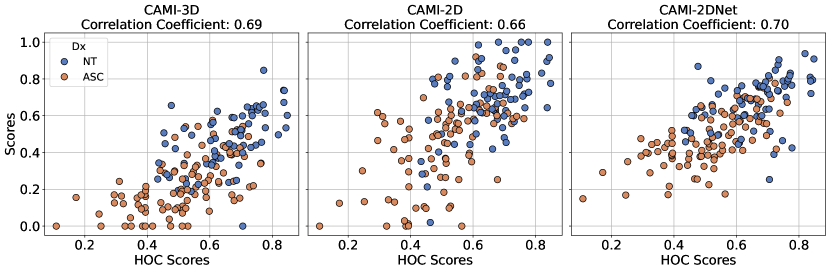
(a)

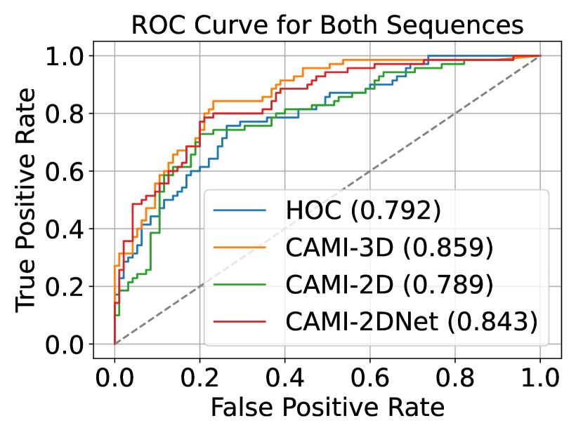
(b)

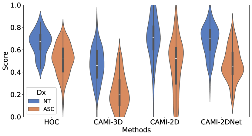
(c)

Figure 2: Comparisons between the CAMI-2DNet, CAMI-2D, CAMI-3D, and human observation coding (HOC) methods using CAMI-47 dataset (27 ASCs, 20 NT). (a) Correlation with HOC Scores: Scatter plots showing the correlation between HOC scores and the scores from CAMI-3D, CAMI-2D, and CAMI-2DNet. The correlation coefficients are 0.69 for CAMI-3D, 0.66 for CAMI-2D, and 0.70 for CAMI-2DNet, indicating that CAMI-2DNet has the highest correlation with HOC scores. (b) ROC Curve for Both Sequences: Receiver operating characteristic (ROC) curve: true positive rate vs. false positive rate as classification threshold is varied. The Area Under the Curve (AUC) indicates the diagnostic ability of the different methods. CAMI-2DNet (AUC = 0.843) demonstrates comparable performance to CAMI-3D (AUC = 0.859) and superior performance over both HOC (AUC = 0.792) and CAMI-2D (AUC = 0.789). (c) Violin Plot of Scores: The violin plots illustrate the distribution of scores for ASC and NT groups across the four methods. CAMI-2DNet not only shows a clear separation between the ASC groups but also displays less variability within each group, highlighting its robustness and reliability.

5.2 Results

5.2.1 Construct Validity and Test Re-test Reliability

To verify the construct validity of our method relative to CAMI-3D and CAMI-2D, we analyzed their correlation with the scores obtained from HOC across all sequences and trials of the CAMI-47 dataset. The results, as illustrated in Figure 2(a), show strong positive correlations between the three methods and HOC. Specifically, the correlation coefficients were 0.69 for CAMI-3D, 0.66 for CAMI-2D, and 0.70 for CAMI-2DNet. Notably, CAMI-2DNet, which operates entirely without supervision from HOC, demonstrated the highest correlation with HOC scores. This strong correlation not only highlights the accuracy and reliability of CAMI-2DNet but also underscores its potential as a highly effective tool for analyzing the participant data independently of HOC supervision.

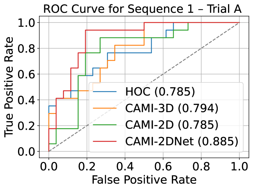
(a)

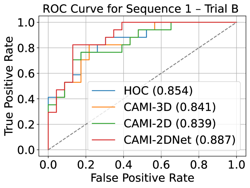
(b)

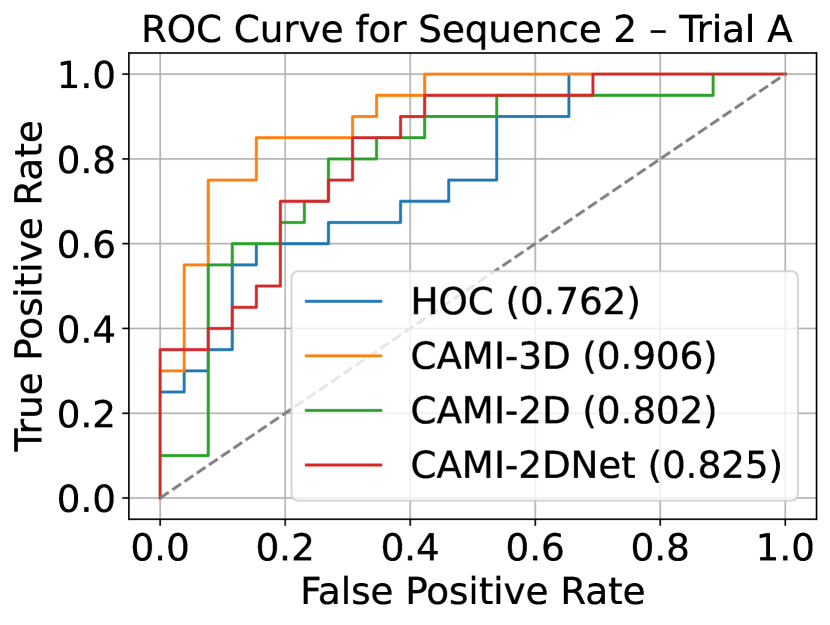
(c)

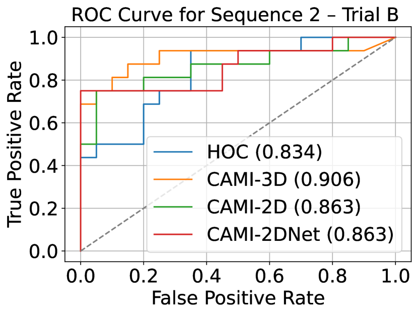
(d)

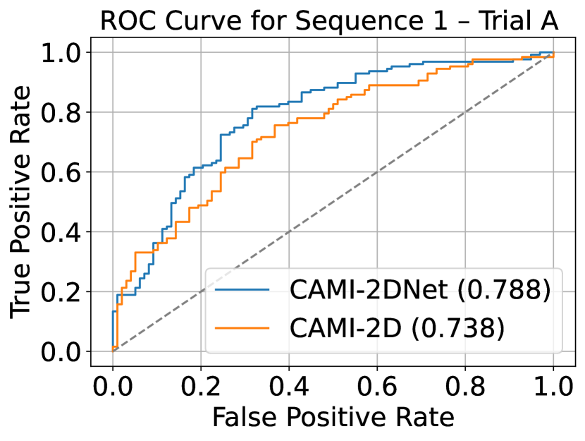
(e)

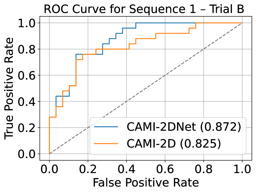
(f)

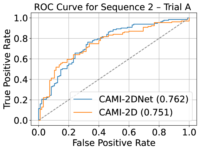
(g)

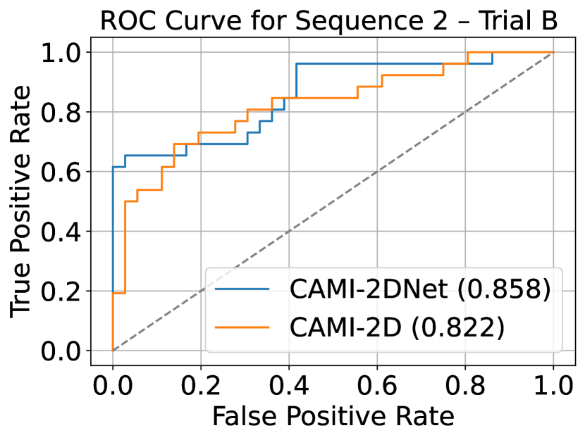
(h)

Figure 3: Receiver Operating Characteristic (ROC) curves comparing the diagnostic performance of HOC, CAMI-3D, CAMI-2D, and CAMI-2DNet across two datasets: CAMI-47 and CAMI-185. The top row (a-d) presents results on the CAMI-47 dataset for two sequences, each consisting of two trials. CAMI-2DNet consistently outperforms HOC and CAMI-2D and demonstrates comparable or superior performance to CAMI-3D. The bottom row (e-h) shows results on the CAMI-185 dataset, comparing CAMI-2DNet with CAMI-2D across two sequences and two trials. CAMI-2DNet achieves higher diagnostic accuracy in all trials, demonstrating a higher AUC than CAMI-2D.

5.2.2 Diagnostic Classification Ability

We evaluated the performance of our method, CAMI-2DNet, relative to CAMI-3D, CAMI-2D, and HOC in classifying children into diagnostic groups by computing the receiver-operating characteristic (ROC) curve across all sequences and trials of the CAMI-47 dataset. Larger areas under the curve (AUC) indicate better discriminative ability, as shown in Figure 2(b). CAMI-3D demonstrated the highest performance with an AUC of 0.859, indicating its superior capability in distinguishing between diagnostic groups. The 3D nature of this method likely contributes to its better performance. The CAMI-2D method, which operates on 2D video data, showed an AUC of 0.789. While its performance is slightly lower than that of CAMI-3D, it provides valuable discriminative ability, comparable to the HOC method (AUC = 0.792). The reliance on 2D data without leveraging the depth information of 3D data might account for this difference. CAMI-2DNet achieved an AUC of 0.843, demonstrating comparable performance to CAMI-3D and superior performance over both CAMI-2D and HOC. CAMI-2DNet’s ability to operate directly on video data without requiring HOC annotations during training offers a significant practical advantage. This makes CAMI-2DNet a highly effective and efficient tool for diagnostic classification, balancing high performance with operational simplicity. Furthermore, the violin plots, in Figure 2(c), showing the distribution of scores for the NT and ASC groups across the four methods, demonstrate that CAMI-2DNet not only exhibits a distinct separation between ASCs and NT groups but also shows relatively reduced variability within each group, underscoring its robustness and reliability.

The ROC curve for both sequences, consisting of two trials in CAMI-47, is shown in Figure 3 (a-d). For instance, in both trials of Sequence 1, CAMI-2DNet achieved the highest AUC (Trial A: 0.885, Trial B: 0.887), outperforming CAMI-3D (Trial A: 0.794, Trial B: 0.84), CAMI-2D (Trial A: 0.785, Trial B: 0.839, and HOC (Trial A: 0.785, Trial B: 0.854). For Sequence 2 - Trial A, CAMI-2DNet achieved an AUC of 0.825, which is higher than CAMI-2D (0.802) and HOC (0.762), but lower than CAMI-3D (0.906). In Sequence 2 - Trial B, CAMI-2DNet and CAMI-2D both achieved an AUC of 0.863, while CAMI-3D scored the highest at 0.906 and HOC obtained 0.834. These trials demonstrate the consistent and high performance of CAMI-2DNet across different sequences and trials, reinforcing its capability as a practical and effective tool for diagnostic classification.

The ROC curves across both sequences and trials in the CAMI-185 dataset further highlight CAMI-2DNet’s consistent superiority compared to CAMI-2D. As shown in Figure 3 (e-h), CAMI-2DNet achieves higher AUC scores in both trials of Sequence 1 (Trial A: 0.787 vs. 0.737, Trial B: 0.853 vs. 0.824) and Sequence 2 (Trial A: 0.767 vs. 0.751, Trial B: 0.856 vs. 0.824). Overall, CAMI-2DNet outperforms CAMI-2D and HOC in terms of diagnostic ability and maintains a strong correlation with HOC scores. Moreover, CAMI-2DNet performs comparably to CAMI-3D while offering greater practicality by operating directly on video data and without needing labor-intensive HOC annotations and ad-hoc normalization steps.

6 Conclusion

We introduced CAMI-2DNet, a scalable and interpretable deep learning-based approach to motor imitation assessment in video data. CAMI-2DNet uses 2D pose estimation techniques to extract 2D joint trajectories from the video. These trajectories are then mapped to a motion representation that is disentangled from nuisance factors such as body shape and camera viewpoint. A motor imitation score is then computed by comparing the motion representation of an individual to that of the actor. Our experiments demonstrate that CAMI-2DNet performs on par with CAMI-3D in discriminating ASC vs neurotypical children, and outperforms both HOC and CAMI-2D, while offering greater practicality by operating directly on video data and without the need for ad-hoc data normalization and HOC annotations. These results highlight CAMI-2DNet as an effective and accessible tool for assessing motor imitation in children with ASCs and related developmental conditions.

7 Model Architecture Details

The encoder-decoder architecture we employed consists of three encoders – Motion Encoder, Body Encoder, and View Encoder – along with a Decoder module as in [19]. Each encoder disentangles a specific aspect of the input pose sequences: motion dynamics, skeletal structure, and camera viewpoint, respectively. The decoder reconstructs the input 2D pose sequence, ensuring that the disentangled representations retain sufficient information to reconstruct the original poses.

Motion Encoder

The Motion Encoder processes the temporal dynamics of input pose sequences. It uses three convolutional layers, each with a kernel size $k=8$ and a stride $s=2$, followed by leaky ReLU (LReLU) activation. All convolutional layers use reflected padding. The input has $2\!\times\!\!J_{\mathcal{S}}$ channels, where $J_{\mathcal{S}}$ represents the number of joints of a body segment $\mathcal{S}$. The number of channels progressively increases to 128, allowing the encoder to extract higher-level motion features at multiple resolutions.

Body Encoder

The Body Encoder disentangles skeletal structure information. It uses convolutional layers with a smaller kernel size $k=7$ and stride $s=1$, followed by max pooling (MP) to downsample spatial features. The third convolutional layer incorporates global max pooling to capture global skeletal structure features. Finally, a $1\times 1$ convolution reduces the dimensionality of the feature maps to 16 channels.

View Encoder

The View Encoder extracts viewpoint-related features, disentangling variations due to camera angles. Similar to the Body Encoder, it applies convolutional layers with $k=7$, followed by average pooling (AP). The third convolutional layer uses global average pooling to summarize viewpoint information globally, and a final $1\times 1$ convolution reduces the output to 8 channels.

Decoder

The Decoder reconstructs the input 2D joint locations from the disentangled motion, skeletal, and viewpoint representations. It consists of three layers that progressively upsample the features. Each layer includes an upsampling operation followed by convolution, dropout, and LReLU activation. Dropout is applied in the first two layers to reduce overfitting and improve generalization. The final layer outputs $2\!\times\!\!J_{\mathcal{S}}$ channels, corresponding to the 2D locations of the $J_{\mathcal{S}}$ joints for a body segment $\mathcal{S}$. Table 1 provides a detailed summary of the encoder-decoder architecture.

Table 1: Network Architecture Summary. The table describes the network structure of the encoder-decoder architecture for disentangling motion, skeletal structure, and viewpoint representations. Conv., LReLU, MP, AP, Upsample, and Dropout denote convolution, leaky ReLU, max pooling, average pooling, upsampling, and dropout layers, respectively. The parameters $k$ and $s$ represent the kernel width and stride, respectively, and the rightmost column reports the number of input and output channels for each layer.

Name	Layers	$k$	$s$	in/out
Motion Encoder	Conv. + LReLU	8	2	($2\!\times\!\!J_{\mathcal{S}}$)/64
	Conv. + LReLU	8	2	64/96
	Conv. + LReLU	8	2	96/128
Body Encoder	Conv. + LReLU + Max Pooling (MP)	7	1	($2\!\times\!\!J_{\mathcal{S}}$)/32
	Conv. + LReLU + MP	7	1	32/48
	Conv. + LReLU + Global MP	7	1	48/64
	Conv.	1	1	64/16
View Encoder	Conv. + LReLU + Average Pooling (AP)	7	1	($2\!\times\!\!J_{\mathcal{S}}$)/32
	Conv. + LReLU + AP	7	1	32/48
	Conv. + LReLU + Global AP	7	1	48/64
	Conv.	1	1	64/8
Decoder	Upsample + Conv. + Dropout + LReLU	7	1	152/128
	Upsample + Conv. + Dropout + LReLU	7	1	128/64
	Upsample + Conv.	7	1	64/($2\!\times\!\!J_{\mathcal{S}}$)

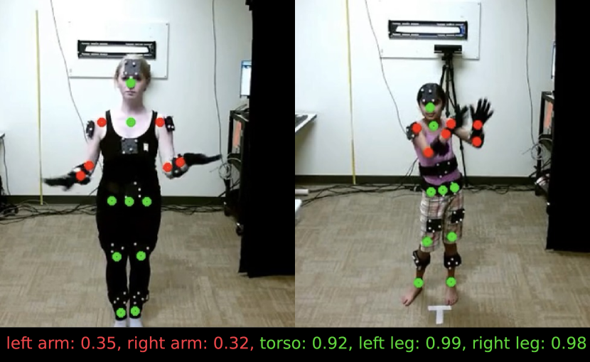
(a)

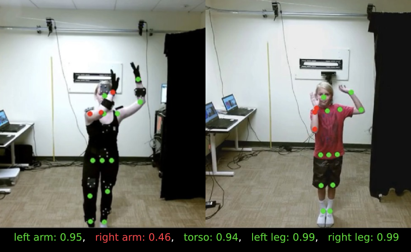
(b)

Figure 4: Visualization of localized motion imitation scores for body segments, comparing the actor (left) and children’s imitation (right). (a) Top: The scores indicate low similarity for arms (left: 0.35, right: 0.32), with high alignment for the torso (0.92), left leg (0.99), and right leg (0.98). (b) Bottom: Higher similarity for the left arm (0.95) but lower for the right arm (0.46). Torso (0.94), left leg (0.99), and right leg (0.99) maintain high alignment. Red highlights low alignment below a threshold, while green indicates high alignment.

8 Interpretable Scores

As discussed in Section 2.2, to enhance the interpretability of motor imitation assessments, CAMI-2DNet localizes the analysis to specific body segments, such as the left arm, right arm, torso, left leg, and right leg. By isolating the imitation performance for each segment, CAMI-2DNet provides detailed insights into which body regions contribute to observed differences in motor imitation. This localized assessment enhances the interpretability of imitation performance, potentially facilitating more targeted interventions. Figure 4 illustrates a snapshot of examples of localized motion imitation scores for two different motions.

References

- [1] H. Over and M. Carpenter, “The social side of imitation,” Child Development Perspectives, vol. 7, pp. 6–11, 2013. [Online]. Available: https://api.semanticscholar.org/CorpusID:145356998
- [2] J. H. G. Williams, A. Whiten, and T. Singh, “A systematic review of action imitation in autistic spectrum disorder,” Journal of Autism and Developmental Disorders, vol. 34, pp. 285–299, 2004. [Online]. Available: https://api.semanticscholar.org/CorpusID:45785161
- [3] S. Michelet, K. Karp, E. Delaherche, C. Achard, and M. Chetouani, “Automatic imitation assessment in interaction,” in International Workshop on Human Behavior Unterstanding, 2012. [Online]. Available: https://api.semanticscholar.org/CorpusID:14011095
- [4] R. C. Schmidt, S. Morr, P. A. Fitzpatrick, and M. J. Richardson, “Measuring the dynamics of interactional synchrony,” Journal of Nonverbal Behavior, vol. 36, pp. 263–279, 2012. [Online]. Available: https://api.semanticscholar.org/CorpusID:144971602
- [5] A. Paxton and R. Dale, “Frame-differencing methods for measuring bodily synchrony in conversation,” Behavior Research Methods, vol. 45, pp. 329 – 343, 2012. [Online]. Available: https://api.semanticscholar.org/CorpusID:8543016
- [6] S. Y. Chun and C.-S. Lee, “Human action recognition using histogram of motion intensity and direction from multiple views,” IET Comput. Vis., vol. 10, pp. 250–256, 2016. [Online]. Available: https://api.semanticscholar.org/CorpusID:33423418
- [7] C.-P. Huang, C.-H. Hsieh, K.-T. Lai, and W.-Y. Huang, “Human action recognition using histogram of oriented gradient of motion history image,” 2011 First International Conference on Instrumentation, Measurement, Computer, Communication and Control, pp. 353–356, 2011. [Online]. Available: https://api.semanticscholar.org/CorpusID:10162344
- [8] R. A. Chaudhry, A. Ravichandran, G. Hager, and R. Vidal, “Histograms of oriented optical flow and binet-cauchy kernels on nonlinear dynamical systems for the recognition of human actions,” 2009 IEEE Conference on Computer Vision and Pattern Recognition, pp. 1932–1939, 2009. [Online]. Available: https://api.semanticscholar.org/CorpusID:123081582
- [9] A. Ravichandran, R. A. Chaudhry, and R. Vidal, “View-invariant dynamic texture recognition using a bag of dynamical systems,” 2009 IEEE Conference on Computer Vision and Pattern Recognition, pp. 1651–1657, 2009. [Online]. Available: https://api.semanticscholar.org/CorpusID:14193472
- [10] B. Tunçgenç, C. Pacheco, R. Rochowiak, R. Nicholas, S. Rengarajan, E. Zou, B. Messenger, R. Vidal, and S. H. Mostofsky, “Computerised assessment of motor imitation (cami) as a scalable method for distinguishing children with autism,” in iol Psychiatry Cogn Neurosci Neuroimaging, 2021. [Online]. Available: https://api.semanticscholar.org/CorpusID:263508051
- [11] R. Bellman and R. E. Kalaba, “On adaptive control processes,” Ire Transactions on Automatic Control, vol. 4, pp. 1–9, 1959. [Online]. Available: https://api.semanticscholar.org/CorpusID:123112075
- [12] R. Santra, C. Pacheco, D. Crocetti, R. Vidal, S. H. Mostofsky, and B. Tunçgenç, “Computerised assessment of motor imitation (cami) identifies autism-specific difficulties not observed in adhd or neurotypical development,” British Journal of Psychiatry, in press.
- [13] Z. Cao, G. Hidalgo, T. Simon, S.-E. Wei, and Y. Sheikh, “Openpose: Realtime multi-person 2d pose estimation using part affinity fields,” IEEE Transactions on Pattern Analysis and Machine Intelligence, vol. 43, pp. 172–186, 2018. [Online]. Available: https://api.semanticscholar.org/CorpusID:198169848
- [14] K. Sun, B. Xiao, D. Liu, and J. Wang, “Deep high-resolution representation learning for human pose estimation,” 2019 IEEE/CVF Conference on Computer Vision and Pattern Recognition (CVPR), pp. 5686–5696, 2019.
- [15] K. A. Kinfu and R. Vidal, “Efficient vision transformer for human pose estimation via patch selection,” in British Machine Vision Conference, 2023. [Online]. Available: https://api.semanticscholar.org/CorpusID:259096162
- [16] D. E. Lidstone, R. Rochowiak, C. Pacheco, B. Tunçgenç, R. Vidal, and S. H. Mostofsky, “Automated and scalable computerized assessment of motor imitation (cami) in children with autism spectrum disorder using a single 2d camera: A pilot study,” Research in Autism Spectrum Disorders, vol. 87, p. 101840, 2021. [Online]. Available: https://api.semanticscholar.org/CorpusID:238658976
- [17] D. Holden, T. Komura, and J. Saito, “Phase-functioned neural networks for character control,” ACM Transactions on Graphics (TOG), vol. 36, pp. 1 – 13, 2017. [Online]. Available: https://api.semanticscholar.org/CorpusID:7261259
- [18] D. Holden, J. Saito, and T. Komura, “A deep learning framework for character motion synthesis and editing,” Seminal Graphics Papers: Pushing the Boundaries, Volume 2, 2016. [Online]. Available: https://api.semanticscholar.org/CorpusID:18149328
- [19] K. Aberman, R. Wu, D. Lischinski, B. Chen, and D. Cohen-Or, “Learning character-agnostic motion for motion retargeting in 2d,” ACM Transactions on Graphics (TOG), vol. 38, pp. 1 – 14, 2019. [Online]. Available: https://api.semanticscholar.org/CorpusID:146120721
- [20] H. Coskun, D. J. Tan, S. Conjeti, N. Navab, and F. Tombari, “Human motion analysis with deep metric learning,” ArXiv, vol. abs/1807.11176, 2018. [Online]. Available: https://api.semanticscholar.org/CorpusID:51880887
- [21] J. Park, S. Cho, D. Kim, O. Bailo, H. Park, S. Hong, and J. Park, “A body part embedding model with datasets for measuring 2d human motion similarity,” IEEE Access, vol. 9, pp. 36 547–36 558, 2021. [Online]. Available: https://api.semanticscholar.org/CorpusID:232152082
- [22] Adobe Systems Inc, “Mixamo.” [Online]. Available: https://www.mixamo.com
- [23] A. P. Association, Diagnostic and Statistical Manual of Mental Disorders, 5th ed. American Psychiatric Association, 2022. [Online]. Available: https://doi.org/10.1176/appi.books.9780890425787
- [24] A. Mccrimmon and K. Rostad, “Test review: Autism diagnostic observation schedule, second edition (ados-2) manual (part ii): Toddler module,” Journal of Psychoeducational Assessment, vol. 32, pp. 88 – 92, 2014. [Online]. Available: https://api.semanticscholar.org/CorpusID:145257612
- [25] T. P. Bruni, “Test review: Social responsiveness scale–second edition (srs-2),” Journal of Psychoeducational Assessment, vol. 32, pp. 365 – 369, 2014. [Online]. Available: https://api.semanticscholar.org/CorpusID:146619745
- [26] L. G. Weiss, V. N. Locke, T. Pan, J. G. Harris, D. H. Saklofske, and A. Prifitera, “Wechsler intelligence scale for children—fifth edition,” WISC-V, 2019. [Online]. Available: https://api.semanticscholar.org/CorpusID:150834011
- [27] S. E. Henderson, D. A. Sugden, and A. L. Barnett, Movement Assessment Battery for Children – Second Edition (MABC-2). London, UK: Pearson Assessment, 2007.
- [28] E. Gowen, “Imitation in autism: why action kinematics matter,” Frontiers in Integrative Neuroscience, vol. 6, 2012. [Online]. Available: https://api.semanticscholar.org/CorpusID:10727495
- [29] L. K. MacNeil and S. H. Mostofsky, “Specificity of dyspraxia in children with autism.” Neuropsychology, vol. 26 2, pp. 165–71, 2012. [Online]. Available: https://api.semanticscholar.org/CorpusID:13944491
- [30] D. McAuliffe, A. S. Pillai, A. Tiedemann, S. H. Mostofsky, and J. B. Ewen, “Dyspraxia in asd: Impaired coordination of movement elements,” Autism Research, vol. 10, 2017. [Online]. Available: https://api.semanticscholar.org/CorpusID:4475753
- [31] R. P. Hobson and J. A. Hobson, “Dissociable aspects of imitation: a study in autism.” Journal of experimental child psychology, vol. 101 3, pp. 170–85, 2008. [Online]. Available: https://api.semanticscholar.org/CorpusID:41120882
- [32] L. E. Marsh, A. Pearson, D. Ropar, and A. F. de C. Hamilton, “Children with autism do not overimitate,” Current Biology, vol. 23, pp. R266–R268, 2013. [Online]. Available: https://api.semanticscholar.org/CorpusID:1817284