Delocalization of a general class of random block Schrödinger operators

Abstract.

We consider a natural class of extensions of the Anderson model on $\mathbb{Z}^{d}$, called random block Schrödinger operators, which feature a random block potential. They are defined on the $d$-dimensional lattice $(\mathbb{Z}/L\mathbb{Z})^{d}$ and take the form $H=V+\lambda\Psi$, where $V$ is a diagonal block matrix with diagonal blocks that are i.i.d. $W^{d}\times W^{d}$ GUE, $\Psi$ describes the interactions between neighboring blocks, and $\lambda>0$ is a coupling parameter. We focus on three specific random block Schrödinger operators: the block Anderson model, where $\Psi$ is the Laplacian operator on $\mathbb{Z}^{d}$; the Anderson orbital model, where $\Psi$ is a block Laplacian operator; the Wegner orbital model, where the nearest-neighbor blocks of $\Psi$ are random matrices. Let $\Lambda_{\Psi}$ denote the strength of interaction between two neighboring blocks. Assuming $d\geq 7$ and $W\geq L^{\varepsilon}$ for a small constant ${\varepsilon}>0$, under the condition $W^{d/4}/\Lambda_{\Psi}\ll\lambda\ll 1$, we prove delocalization and quantum unique ergodicity for the bulk eigenvectors, as well as a quantum diffusion estimate for the Green’s function. Together with the localization result proved in [44], our results rigorously establish an Anderson localization-delocalization transition of the random block Schrödinger operators as $\lambda$ varies.

Our proof is based on a nontrivial extension of the $T$-expansion method and the concept of self-energy renormalization developed for random band matrices [55, 56, 54]. Additionally, we explore a conceptually new idea called coupling renormalization in our proof. This phenomenon extends the self-energy renormalization and is prevalent in quantum field theory, yet it is identified here for the first time within the context of random Schrödinger operators. We anticipate that our techniques can be adapted to real or non-Gaussian block potentials and more general interactions $\Psi$.

1. Introduction

The random Schrödinger operator or, more specifically, the Anderson model [9], is a significant framework for describing the spectral and transport properties of disordered media, such as the behavior of moving electrons in a metal with impurities. Mathematically, the $d$-dimensional Anderson model is defined by a random Hamiltonian on $\ell^{2}(\mathbb{Z}^{d})$:

$$H=-\Delta+\delta V$$ (1.1)

where $\Delta$ is the Laplacian operator on $\mathbb{Z}^{d}$, $V$ is a random potential with i.i.d. random diagonal entries, and $\delta>0$ is a coupling parameter describing the strength of the disorder. The Anderson model exhibits a localization-delocalization transition that depends on the energy, dimension, and disorder strength, capturing the physical phenomenon of metal-insulator transition in disordered quantum systems. In the strong disorder regime, where $\delta$ is large, the eigenvectors of the Anderson model are expected to be exponentially localized. Conversely, in the weak disorder regime, it is conjectured that for dimensions $d\geq 3$, there exist mobility edges that separate the localized and delocalized phases; particularly, within the bulk of the spectrum, the eigenvectors are expected to be completely delocalized.

The localization phenomenon of the 1D Anderson model has long been well understood; see e.g., [34, 40, 13, 19] among many other references. Studying the Anderson model in higher dimensions ($d\geq 2$) is significantly more challenging. The first rigorous localization result was established by Fröhlich and Spencer [31] using multi-scale analysis. A simpler alternative proof was later provided by Aizenman and Molchanov [3] using a fractional moment method. In dimension $d=2$, Anderson localization is expected to occur at all energies when $\delta>0$ [1]. Numerous remarkable results have been proven concerning the localization of the Anderson model in dimensions $d\geq 2$ (see, e.g., [30, 14, 46, 2, 12, 33, 20, 41]), but the above conjecture remains open. For more extensive reviews and related references, we direct readers to [39, 49, 47, 7, 37].

On the other hand, our understanding of delocalization in the Anderson model for dimensions $d\geq 3$ is even more limited—almost nonexistent. To date, the existence of a delocalized regime has only been proved for the Anderson model on Bethe lattice [5, 6], but not for any finite-dimensional integer lattice $\mathbb{Z}^{d}$. In this paper, we make an effort toward addressing the Anderson delocalization conjecture by considering a natural variant of the random Schrödinger operator—the random block Schrödinger operator (RBSO), which is formed by replacing the i.i.d. potential with i.i.d. block potential. More precisely, we define RBSO, denoted by $H$, on a $d$-dimensional lattice $\mathbb{Z}_{L}^{d}:=\{1,2,\cdots,L\}^{d}$ of linear size $L$. We decompose $\mathbb{Z}_{L}^{d}$ into $n^{d}$ disjoint boxes of side length $W$ (with $L=nW$). Corresponding to these boxes, we define $V$ as a diagonal block matrix, with blocks being i.i.d. $W^{d}\times W^{d}$ random matrices. For simplicity, we assume these random matrices are drawn from GUE (Gaussian unitary ensemble), but this assumption is not essential for us.

From a physical perspective, our new RBSO is related to the Anderson model on the lattice $\mathbb{Z}_{n}^{d}$ through a coarse graining transformation, and we refer to it as the “block Anderson model” in this paper. Motivated by the work of Wegner [52] and its continuation in [45, 43], we also consider another type of RBSO that models the motion of a quantum particle with multiple internal degrees of freedom (referred to as orbits or spin) in a disordered medium. In other words, the quantum particle moves according to the Anderson model on $\mathbb{Z}_{n}^{d}$, while its spin either remains unchanged or rotates randomly as the particle hops between sites on $\mathbb{Z}_{n}^{d}$. In the former scenario, we call it the “Anderson orbital model”, while in the latter, it is known as the celebrated “Wegner orbital model”. We rescale (1.1) by $\lambda:=\delta^{-1}$ and replace the interaction term $-\lambda\Delta$ with a more general (deterministic or random) matrix $\lambda\Psi$ that models interactions between neighboring blocks. In this paper, we will study RBSO $H=\lambda\Psi+V$ that represents the above three models. We have chosen to focus on these three models for the sake of clarity in presentation; however, the specific forms of $\Psi$ are not crucial to our results, see Remark 1.3 below.

A major advantage of RBSO over the Anderson model is that it contains significantly more random entries. While approaching the delocalized regime of the Anderson model is challenging with only $N=L^{d}$ random entries in $V$, we will show that $N^{1+{\varepsilon}}$ random entries in the block potential of our RBSO are already sufficient for proving Anderson delocalization in high dimensions, even in the presence of strong disorder. More precisely, suppose $d\geq 7$ and $W\geq L^{\varepsilon}$ for an arbitrarily small constant ${\varepsilon}>0$. We prove that as long as $\delta$ is sufficiently “small” ($\delta\ll W^{d/4-1}$ for the block Anderson model and $\delta\ll W^{d/4}$ for the Anderson orbital and Wegner orbital models), the bulk eigenvectors of $H$ are delocalized and satisfy a quantum unique ergodicity (QUE) estimate. Moreover, we show that the evolution of the particle behaves diffusively up to the Thouless time (defined in (1.17) below). It has been established in [44] that the Anderson orbital and Wegner orbital models are localized when $\delta\gg W^{d/2}$. Thus, our results rigorously establish, for the first time in the literature, an Anderson localization-delocalization transition for a certain class of finite-dimensional random Schrödinger operators as the interaction strength varies. We believe that if the condition $W\geq L^{\varepsilon}$ can be relaxed to $W\geq C$ for a large but finite constant $C>0$, the delocalization conjecture for the Anderson model would be (almost) within reach.

Our RBSO serves as a natural interpolation between random Schrödinger operators and Wigner random matrices [53] as $W$ increases from 1 to $L$. Another well-known interpolation is the celebrated random band matrix (RBM) ensemble [16, 15, 32] defined on $\mathbb{Z}_{L}^{d}$. The RBM is a Wigner-type random matrix $(H_{xy})_{x,y\in\mathbb{Z}_{L}^{d}}$ such that $H_{xy}$ is non-negligible only when $|x-y|\leq W$, with $W$ being the band width. Over the past decade, significant progress has been made in understanding both the localization and delocalization of RBMs in all dimensions. We refer the reader to [10, 11, 18, 55] for a brief review of relevant references. A recent breakthrough [57] established the delocalization of 1D random band matrices under the sharp condition $W\gg L^{1/2}$ on band width. So far, the best delocalization result for higher-dimensional band matrices was achieved in a series of papers [55, 56, 54], which proved that if $d\geq 7$ and $W\geq L^{\varepsilon}$ for an arbitrarily small constant ${\varepsilon}>0$, the bulk eigenvectors of RBM are delocalized.

The proof in this paper is based on a (quite nontrivial) extension of the ideas in [55, 56, 54]. Note that RBM can be regarded as a special case of RBSO with $\lambda=1$ and $\Psi$ obtained by setting the diagonal blocks of a $d$-dimensional RBM to 0. Despite the similarities between RBSOs and RBMs, there are some technical differences: our RBSO lacks the translation symmetry present in the RBM considered in [55, 56, 54]; the deterministic limit of the Green’s function of RBSO takes a more complicated form, which is no longer a scalar matrix (see (2.3) below); the graphical tools and expansions involving RBSO are also more complex than those for RBM. These differences introduce technical challenges that complicate the proofs. For instance, we will demonstrate that the block translation symmetry of our RBSO compensates for the loss of translation symmetry. However, a more crucial difference between our RBSO and RBM lies in the additional parameter $\lambda$ before $\Psi$. Since we are interested in the delocalization of RBSO under interactions that are as weak as possible, the parameter $\lambda$ will be small and tends to 0 as $W\to\infty$. Consequently, the Green’s function of RBSO diffuses more slowly than RBM. For instance, (2.42) below demonstrates that the diffusion constant is smaller than that of RBM by a small factor $\beta(\lambda)^{-1}$, where $\beta(\lambda)$ will be defined in (1.16) below. If we were to apply the method developed in [55, 56, 54] naively, some of our graphs would contain additional powers of $\beta(\lambda)$. This would lead to a significantly worse continuity estimate, ultimately rendering our proof invalid.

To address the aforementioned issue, we discover a new mechanism called coupling (or vertex) renormalization. We have borrowed this term from Quantum Field Theory (QFT). Roughly speaking, coupling renormalization is a common phenomenon in QFT that describes a cancellation mechanism occurring when calculating the interactions of several propagators using Feynman diagrams. In the setting of RBSO, where propagators correspond to entries of the Green’s function, we encounter a similar scenario: when calculating the expectation of the product of Green’s function entries, we will get several graphs with these propagators coupled at a specific “vertex”. Upon summing these graphs, we find that they cancel each other remarkably, resulting in a vanishing factor. For a more detailed discussion of this phenomenon and some basic ideas behind its proof, we refer readers to Section 1.3 below.

1.1. The model

For definiteness, throughout this paper, we assume that $L=nW$ for some $n,W\in 2\mathbb{N}+1$. Then, we choose the center of the lattice as $0$. However, our results still hold for even $n$ or $W$, as long as we choose a different center for the lattice. Consider a cube of linear size $L$ in $\mathbb{Z}^{d}$, i.e.,

$$\mathbb{Z}_{L}^{d}:=[\![{-(L-1)/2,(L-1)/2}]\!]^{d}.$$ (1.2)

Hereafter, for any $a,b\in\mathbb{R}$, we denote $\llbracket a,b\rrbracket:=[a,b]\cap\mathbb{Z}$. We will view $\mathbb{Z}_{L}^{d}$ as a torus and denote by $({x-y})_{L}$ the representative of $x-y$ in $\mathbb{Z}_{L}^{d}$, i.e.,

$$({x-y})_{L}:=\left((x-y)+L\mathbb{Z}^{d}\right)\cap\mathbb{Z}_{L}^{d}.$$ (1.3)

Now, we impose a block structure on $\mathbb{Z}_{L}^{d}$ with blocks of side length $W$.

Definition 1.1 (Lattice of blocks).

Fix any $d\in\mathbb{N}$. Suppose $L=nW$ for some integers $n,W\in 2\mathbb{N}+1$. We divide $\mathbb{Z}_{L}^{d}$ into $n^{d}$ cubic blocks of side length $W$, such that the central one is $[\![{-(W-1)/2,(W-1)/2}]\!]^{d}$. Given any $x\in\mathbb{Z}_{L}^{d}$, denote the block containing $x$ by $[x]$. Denote the lattice of blocks $[x]$ by $\widetilde{\mathbb{Z}}_{n}^{d}$. We will view $\widetilde{\mathbb{Z}}_{n}^{d}$ as a torus and denote by $({[x]-[y]})_{n}$ the representative of $[x]-[y]$ in $\widetilde{\mathbb{Z}}_{n}^{d}$. For convenience, we will regard $[x]$ both as a vertex of the lattice $\widetilde{\mathbb{Z}}_{n}^{d}$ and a subset of vertices on the lattice $\mathbb{Z}_{L}^{d}$. Denote by $\{x\}$ the representative of $x$ in the cubic block $[0]$ containing the origin, i.e.,

$$\{x\}:=(x+W\mathbb{Z}^{d})\cap[0]=x-W[x].$$

For any $x\in\mathbb{Z}_{L}^{d}$, we define the projections $\pi_{L\to n}:\mathbb{Z}_{L}^{d}\to\widetilde{\mathbb{Z}}_{n}^{d}$ and $\pi_{L\to W}:\mathbb{Z}_{L}^{d}\to[0]$ such that $\pi_{L\to n}(x)=[x]$ and $\pi_{L\to W}(x)=\{x\}$.

Any $x\in\mathbb{Z}_{L}^{d}$ can be labelled as $([x],\{x\})$. Correspondingly, we define the tensor product of two vectors ${\bf{u}}$ and ${\bf{v}}$ with entries indexed by the vertices of $\widetilde{\mathbb{Z}}_{n}^{d}$ and $[0]$, respectively, as

$${\bf{u}}\otimes{\bf{v}}(x):={\bf{u}}([x]){\bf{v}}(\{x\}),\quad x\in\mathbb{Z}_{L}^{d}.$$ (1.4)

Correspondingly, the tensor product of matrices $A_{n}$ and $A_{W}$ defined on $\widetilde{\mathbb{Z}}_{n}^{d}$ and $[0]$, respectively, is given by

$$A_{n}\otimes A_{W}({\bf{u}}\otimes{\bf{v}}):=(A_{n}{\bf{u}})\otimes(A_{W}{\bf{v}}).$$ (1.5)

Clearly, $\|x-y\|_{L}:=\|({x-y})_{L}\|$ is a periodic distance on $\mathbb{Z}_{L}^{d}$ for any norm $\|\cdot\|$ on $\mathbb{Z}^{d}$. For definiteness, we use the $\ell^{1}$-norm in this paper, i.e., $\|x-y\|_{L}:=\|({x-y})_{L}\|_{1}$, which is also the graph distance on $\mathbb{Z}_{L}^{d}$. Similarly, we also define the periodic $\ell^{1}$-distance $\|\cdot\|_{n}$ on $\widetilde{\mathbb{Z}}_{n}^{d}$. For simplicity, throughout this paper, we will abbreviate

$$|x-y|\equiv\|x-y\|_{L},\quad \langle x-y\rangle\equiv\|x-y\|_{L}+W,\quad\text{for}\ \ x,y\in\mathbb{Z}_{L}^{d},$$ (1.6)

$$|[x]-[y]|\equiv\|[x]-[y]\|_{n},\quad \langle[x]-[y]\rangle\equiv\|[x]-[y]\|_{n}+1,\quad\text{for}\ \ x,y\in\widetilde{\mathbb{Z}}_{n}^{d}.$$ (1.7)

We use $x\sim y$ to mean that $x$ and $y$ are neighbors on $\mathbb{Z}_{L}^{d}$, i.e., $|x-y|=1$. Similarly, $[x]\sim[y]$ means that $[x]$ and $[y]$ are neighbors on $\widetilde{\mathbb{Z}}_{n}^{d}$.

Definition 1.2 (Random block Schrödinger operator).

We define an $N\times N$ ($N=L^{d}$) complex Hermitian block random matrix $V$ whose entries are independent Gaussian random variables up to the Hermitian condition $V_{xy}=\overline{V}_{yx}$. Specifically, the off-diagonal entries of $V$ are complex Gaussian random variables:

$$V_{xy}\sim{\cal N}_{\mathbb{C}}(0,s_{xy})\quad\text{with}\quad s_{xy}:=W^{-d}{\bf 1}\left([x]=[y]\right),\quad\text{for}\ \ x\neq y;$$ (1.8)

the diagonal entries of $V$ are real Gaussian random variables distributed as ${\cal N}_{\mathbb{R}}(0,W^{-d})$. In other words, $V$ is a diagonal block matrix with i.i.d. GUE blocks. We will call $V$ a $d$-dimensional “block potential”. Then, we define a general class of random Hamiltonian as

$$H\equiv H({\lambda}):=\lambda\Psi+V,$$ (1.9)

where $\lambda>0$ is a deterministic parameter and $\Psi$ is the interaction Hamiltonian introducing hopping between different blocks. For definiteness, we consider the following three types of $\Psi$ in this paper.

• Block Anderson ($\mathrm{BA}$) model. $\Psi^{\mathrm{BA}}:=2dI_{L}-\Delta_{L}$, where $\Delta_{L}$ denotes the graph Laplacian on $\mathbb{Z}_{L}^{d}$ and $I_{L}$ denotes the $L^{d}\times L^{d}$ identity matrix. In other words, we let $\Psi^{\mathrm{BA}}_{xy}=\mathbf{1}(x\sim y)$ for $x,y\in\mathbb{Z}_{L}^{d}$.

• Anderson orbital ($\mathrm{AO}$) model. $\Psi^{\mathrm{AO}}:=(2dI_{n}-\Delta_{n})\otimes I_{W}$, where $\Delta_{n}$ denotes the graph Laplacian on $\widetilde{\mathbb{Z}}_{n}^{d}$ and $I_{W}$ denotes the $W^{d}\times W^{d}$ identity matrix.

• Wegner orbital ($\mathrm{WO}$) model. The neighboring blocks of $\Psi^{\mathrm{WO}}$ are independent blocks of $W^{d}\times W^{d}$ complex Ginibre matrices up to the Hermitian symmetry $\Psi^{\mathrm{WO}}=(\Psi^{\mathrm{WO}})^{\dagger}$. In other words, the entries of $\Psi$ are independent complex Gaussian random variables up to the Hermitian symmetry:

  $$\Psi_{xy}\sim{\cal N}_{\mathbb{C}}(0,s^{\prime}_{xy}),\quad\text{with}\quad s^{\prime}_{xy}:=W^{-d}{\bf 1}\left([x]\sim[y]\right).$$ (1.10)

We will call $H$ a $d$-dimensional block Anderson/Anderson orbital/Wegner orbital model with linear size $L$, block size $W$, and coupling parameter $\lambda$. For simplicity of presentation, with a slight abuse of notations, we will often use consistent notations for some quantities (e.g., $\Psi$) that are used in all three models. When we want to make the specific model we refer to clear, we will add the super-index $\mathrm{BA}$, $\mathrm{AO}$, or $\mathrm{WO}$.

Remark 1.3.

We remark that in [44], the Anderson orbital model in (ii) is called the “block Anderson model”. In this paper, however, we have adopted the name “Anderson orbital” to distinguish it from our block Anderson model in (i). In this paper, we have chosen three of the most classical representatives in the physics literature. In particular, they represent some general families of RBSOs that exhibit the following features: deterministic interactions that are translation-invariant (block Anderson model), deterministic interactions that are translation-invariant on the block level (Anderson orbital model), and random interactions whose distribution is translation-invariant on the block level (Wegner orbital model). The results and proofs of this paper can be extended to more general random block models that exhibit the metal-insulator transition. Specifically, we expect our method can be applied to deal with almost arbitrary deterministic or random interactions that exhibit block translation symmetry. However, due to length constraints, we do not pursue such directions in the current paper.

1.2. Overview of the main results

In this subsection, we provide a brief overview of our main results. First, we state the localization of our block models. We define the Green’s function (or resolvent) of the Hamiltonian $H$ as

$$G(z):=(H-z)^{-1}=\left(\lambda\Psi+V-z\right)^{-1},\quad z\in\mathbb{C}.$$ (1.11)

Note that since the entries of $H$ have continuous density, $G(z)$ is well-defined almost surely even when $z\in\mathbb{R}$. Utilizing the fractional moment method [3], it was proved in [44] that the fractional moments of the $G$ entries are exponentially localized for small enough $\lambda$. To state the result, we introduce the quantity

$$\Lambda_{\Psi}:=\left(\mathbb{E}\|\Psi_{[x][y]}\|_{HS}^{2}\right)^{1/2},$$

for two blocks $[x]\sim[y]$ on $\widetilde{\mathbb{Z}}_{n}^{d}$, which describes the interaction strength between two neighboring blocks. Here, $\Psi_{[x][y]}=(\Psi_{ab}:a\in[x],b\in[y])$ denotes the $W^{d}\times W^{d}$ block of $\Psi$ with the row and column indices belonging to $[x]$ and $[y]$, respectively. Due to the block translation symmetry of the three models, we notice that $\Lambda_{\Psi}$ does not depend on the choices of the blocks $[x]$ and $[y]$. Through a simple calculation, we find that

$$\Lambda_{\Psi}=\begin{cases}W^{(d-1)/2},&\text{for}\ \Psi=\Psi^{\mathrm{BA}}\\ W^{d/2},&\text{for}\ \Psi\in\{\Psi^{\mathrm{AO}},\Psi^{\mathrm{WO}}\}\end{cases}$$

Theorem 1.4 (Localization).

Consider the models $H$ in Definition 1.2. Fix any $d\geq 1$ and $s\in(0,1)$, there exists a constant $c_{s,d}>0$ such that the following holds. When

$$\lambda\leq c_{s,d}/\Lambda_{\Psi},$$ (1.12)

there exists a constant $C_{s,d}>0$ such that for all $W,L\geq 1$ and $z\in\mathbb{R}$,

$$\mathbb{E}|G_{xy}(z)|^{s}\leq C_{s,d}\Lambda_{\Psi}^{s}\left(\lambda C_{s,d}\Lambda_{\Psi}\right)^{s|[x]-[y]|}.$$ (1.13)

Proof.

The bound (1.13) has been established in [44] for the Anderson orbital and Wegner orbital models. The same argument extends to the block Anderson model by using the facts that the off-diagonal blocks of $\Psi^{\mathrm{BA}}$ are of rank $W^{d-1}$ (in contrast to $W^{d}$ for $\Psi^{\mathrm{AO}}$ and $\Psi^{\mathrm{WO}}$). For simplicity of presentation, we do not provide the details here. ∎

By Theorem 1.4, if we take $\lambda\leq c/\Lambda_{\Psi}$ for a constant $0<c<c_{s,d}\wedge C_{s,d}^{-1}$, then the estimate (1.13) gives the exponential decay of $\mathbb{E}|G_{xy}(z)|^{s}$, from which we readily derive the localization of eigenvectors by [4, Theorem A.1]. It is possible to relax the Gaussian assumption on the entries of $V$ to more general distributions with densities and finite high moments, but we do not pursue this direction in the current paper. On the other hand, if the entries of $V$ are discrete random variables, then proving Anderson localization seems to be much more challenging (see e.g., the Anderson-Bernoulli model considered in [12, 20, 41]).

One main result of this paper gives a counterpart of the above localization result. By extending the methods developed in the recent series [54, 55, 56], we will establish the following results when $d\geq 7$ and $W\geq L^{\varepsilon}$ for a small constant ${\varepsilon}>0$. Roughly speaking, for the models in Definition 1.2, assuming that

$$\lambda\gg W^{d/4}/\Lambda_{\Psi},$$ (1.14)

we will prove that:

• Local law (Theorem 2.2). Within the bulk of the spectrum, we establish a sharp local law for the Green’s function $G(z)$ for $\operatorname{{\mathrm{Im}}}z$ down to the scale

  $$\eta_{*}:=\frac{1}{\beta(\lambda)}\frac{W^{d-5}}{L^{d-5}},$$ (1.15)

  where the parameter $\beta(\lambda)$ is defined as

  $$\beta(\lambda):=\frac{W^{d}}{\lambda^{2}\Lambda_{\Psi}^{2}}=\begin{cases}W/\lambda^{2},&\text{for}\ \Psi=\Psi^{\mathrm{BA}}\\ \lambda^{-2},&\text{for}\ \Psi\in\{\Psi^{\mathrm{AO}},\Psi^{\mathrm{WO}}\}\end{cases}.$$ (1.16)

• Delocalization (Corollary 2.3). For any small constant ${\varepsilon}>0$, most bulk eigenvectors of $H$ have localization length $\geq L^{1-{\varepsilon}}$ with probability $1-\operatorname{o}(1)$.

• Quantum unique ergodicity (QUE, Theorem 2.4). Under certain conditions, there exists a constant ${\varepsilon}>0$ such that with probability $1-\operatorname{o}(1)$, every bulk eigenvector is almost “flat” on all scales $\Omega(L^{1-{\varepsilon}})$. As a consequence, it implies that the localization length of each bulk eigenvector is indeed equal to $L$.

• Quantum diffusion (Theorem 2.6). The evolution of the particle follows a quantum diffusion up to the Thouless time. Here, the Thouless time [21, 51, 48] is defined to be the typical time scale for a particle to reach the boundary of the system. For our models, it is given by

  $$t_{Th}=\beta(\lambda){L^{2}}/{W^{2}}.$$ (1.17)

We refer readers to Section 2 below for more precise statements of these results. Together with Theorem 1.4, our results imply the Anderson metal-insulator transition of the RBSOs in Definition 1.2 as $\lambda$ increases from $\Lambda_{\Psi}^{-1}$ to $W^{d/4}\Lambda_{\Psi}^{-1}$. We conjecture that $\lambda_{c}=\Lambda_{\Psi}^{-1}$ represents the correct threshold for the Anderson transition of our RBSOs (see the discussions below (2.43) for heuristic reasoning).

To facilitate the presentation, we introduce some necessary notations that will be used throughout this paper. We will use the set of natural numbers $\mathbb{N}=\{1,2,3,\ldots\}$ and the upper half complex plane $\mathbb{C}_{+}:=\{z\in\mathbb{C}:\operatorname{{\mathrm{Im}}}z>0\}$. We use superscripts ‘$-$’ and ‘${\dagger}$’ to denote the complex conjugate and Hermitian conjugate of matrices, respectively, i.e., $A^{-}_{xy}:=\overline{A}_{xy}$ and $A^{\dagger}_{xy}:=\overline{A}_{yx}.$ As a convention, we denote $A^{\emptyset}=A$. In this paper, we are interested in the asymptotic regime with $L,W\to\infty$. When we refer to a constant, it will not depend on $L$, $W$, or $\lambda$. Unless otherwise noted, we will use $C$, $D$ etc. to denote large positive constants, whose values may change from line to line. Similarly, we will use $\epsilon$, $\tau$, $c$, ${\mathfrak{c}}$, ${\mathfrak{d}}$ etc. to denote small positive constants. For any two (possibly complex) sequences $a_{L}$ and $b_{L}$ depending on $L$, $a_{L}=\operatorname{O}(b_{L})$, $b_{L}=\Omega(a_{L})$, or $a_{L}\lesssim b_{L}$ means that $|a_{L}|\leq C|b_{L}|$ for some constant $C>0$, whereas $a_{L}=\operatorname{o}(b_{L})$ or $|a_{L}|\ll|b_{L}|$ means that $|a_{L}|/|b_{L}|\to 0$ as $L\to\infty$. We say that $a_{L}\asymp b_{L}$ if $a_{L}=\operatorname{O}(b_{L})$ and $b_{L}=\operatorname{O}(a_{L})$. For any $a,b\in\mathbb{R}$, $a\leq b$, we denote $\llbracket a,b\rrbracket:=[a,b]\cap\mathbb{Z}$, $\llbracket{a}\rrbracket:=\llbracket{1,a}\rrbracket$, $a\vee b:=\max\{a,b\}$, and $a\wedge b:=\min\{a,b\}$. For an event $\Xi$, we let $\mathbf{1}_{\Xi}$ or $\mathbf{1}(\Xi)$ denote its indicator function. For any graph (or lattice), we use $x\sim y$ to mean two vertices $x,y$ are neighbors. Given a vector $\mathbf{v}$, $|\mathbf{v}|\equiv\|\mathbf{v}\|_{2}$ denotes the Euclidean norm and $\|\mathbf{v}\|_{p}$ denotes the $\ell^{p}$-norm. Given a matrix $\cal A=(\cal A_{ij})$, $\|\cal A\|$ and $\|\cal A\|_{\max}:=\max_{i,j}|\cal A_{ij}|$ denote the operator norm and maximum norm, respectively. We will use $\cal A_{ij}$ and $\cal A(i,j)$ interchangeably in this paper.

For simplicity of notation, throughout this paper, we will use the following convenient notion of stochastic domination introduced in [22].

Definition 1.5 (Stochastic domination and high probability event).

(i) Let

$$\xi=\left(\xi^{(W)}(u):W\in\mathbb{N},u\in U^{(W)}\right),\quad\zeta=\left(\zeta^{(W)}(u):W\in\mathbb{N},u\in U^{(W)}\right),$$

be two families of non-negative random variables, where $U^{(W)}$ is a possibly $W$-dependent parameter set. We say $\xi$ is stochastically dominated by $\zeta$, uniformly in $u$, if for any fixed (small) $\tau>0$ and (large) $D>0$,

$$\mathbb{P}\bigg{[}\bigcup_{u\in U^{(W)}}\left\{\xi^{(W)}(u)>W^{\tau}\zeta^{(W)}(u)\right\}\bigg{]}\leq W^{-D}$$

for large enough $W\geq W_{0}(\tau,D)$, and we will use the notation $\xi\prec\zeta$. If for some complex family $\xi$ we have $|\xi|\prec\zeta$, then we will also write $\xi\prec\zeta$ or $\xi=\operatorname{O}_{\prec}(\zeta)$.

(ii) As a convention, for two deterministic non-negative quantities $\xi$ and $\zeta$, we will write $\xi\prec\zeta$ if and only if $\xi\leq W^{\tau}\zeta$ for any constant $\tau>0$.

(iii) We say that an event $\Xi$ holds with high probability (w.h.p.) if for any constant $D>0$, $\mathbb{P}(\Xi)\geq 1-W^{-D}$ for large enough $W$. More generally, we say that an event $\Omega$ holds $w.h.p.$ in $\Xi$ if for any constant $D>0$, $\mathbb{P}(\Xi\setminus\Omega)\leq W^{-D}$ for large enough $W$.

The following classical Ward’s identity, which follows from a simple algebraic calculation, will be used tacitly throughout this paper.

Lemma 1.6 (Ward’s identity).

Let $\cal A$ be a Hermitian matrix. Define its resolvent as $R(z):=(\cal A-z)^{-1}$ for any $z=E+\mathrm{i}\eta\in\mathbb{C}_{+}$. Then, we have

$$\begin{split}\sum_{x}\overline{R_{xy^{\prime}}}R_{xy}=\frac{R_{y^{\prime}y}-\overline{R_{yy^{\prime}}}}{2\mathrm{i}\eta},\quad\sum_{x}\overline{R_{y^{\prime}x}}R_{yx}=\frac{R_{yy^{\prime}}-\overline{R_{y^{\prime}y}}}{2\mathrm{i}\eta}.\end{split}$$ (1.18)

As a special case, if $y=y^{\prime}$, we have

$$\sum_{x}|R_{xy}(z)|^{2}=\sum_{x}|R_{yx}(z)|^{2}=\frac{\operatorname{{\mathrm{Im}}}R_{yy}(z)}{\eta}.$$ (1.19)

1.3. Coupling renormalization

In this subsection, we briefly describe some basic ideas regarding the coupling (or vertex) renormalization mechanism utilized in our proof. When evaluating the propagator $|G_{xy}|^{2}$ for RBMs in [55], we identify a self-energy renormalization mechanism, which also applies to our RBSO. Roughly speaking, we will derive an expansion of $|G_{xy}|^{2}$ (up to some small errors) as follows:

In this picture, the blue and red edges correspond to the $G_{xy}$ and $\overline{G}_{xy}$ edges, respectively. The black double-line edges represent entries of the diffusive matrix defined in (2.21) below, while the gray disk denotes a deterministic matrix $\Sigma$, referred to as the self-energy in the context of QFT. The self-energy arises from “self-interactions” of $|G_{xy}|^{2}$, which is known as the dressed propagator in QFT (with the double-line edge denoting a bare propagator).

On the other hand, coupling renormalization occurs when we evaluate the product of several Green’s function entries, as illustrated in the following picture:

(1.20)

The left-hand side (LHS) represents the product of $|G_{xy}|^{2}$ with four other $G$ edges. Expanding the propagator $|G_{xy}|^{2}$ may lead to three possible scenarios on the right-hand side (RHS): (1) only self-interactions occur between $x$ and $y$, without involving other $G$ edges; (2) $|G_{xy}|^{2}$ and two other $G$ edges couple at a “vertex” $X_{4}$ (the “4” indicates that the vertex involves 4 edges in the original graph); (3) $|G_{xy}|^{2}$ and four other $G$ edges couple at a “vertex” $X_{6}$. We remark that $X_{4}$ and $X_{6}$ are not true vertices in our graphs; rather, each represents a subgraph (often referred to as a “vertex function” in QFT) with several vertices that vary on the local scale $W$. We refer to $X_{4}$ and $X_{6}$ as “molecules” in this paper, as defined in Definition 3.14 below. We find that summing over the graphs in scenario (2) (resp. scenario (3)) results in the cancellation of the subgraphs within molecule $X_{4}$ (resp. $X_{6}$). This gives the desired coupling/vertex renormalization.

We note that while coupling renormalization may seem like a strictly stronger generalization of self-energy renormalization, this is actually not the case. Coupling renormalization occurs at the level of a single molecule, whereas self-energy involves deterministic subgraphs consisting of multiple molecules that vary on the global scale $L$. Hence, coupling renormalization indeed constitutes a cancellation of vertex functions at molecules, while self-energy renormalization involves a more intricate sum zero property (see Definition 3.20 below). It is quite possible that a more general “coupling renormalization” mechanism involving multiple molecules could also apply to our model. However, while exploring this possibility is intriguing in its own right, it does not lead to an improvement in our results or a relaxation of the assumptions.

To understand why coupling renormalization occurs, we consider an $N\times N$ Wigner matrix, which can be viewed as a special case of our RBSO with $W=L$. (In fact, our proof of coupling renormalization for RBSO is based on a comparison between the “local behaviors” of RBSO and Wigner matrices.) We examine the following loop graph consisting of four edges representing the Green’s function entries of a Wigner matrix.

Consider an arbitrary $z=E+\mathrm{i}\eta$ in the bulk of the spectrum, with $|E|\leq 2-\kappa$ for a constant $\kappa>0$ and $\eta\gg N^{-1}$. Through a systematic expansion of the loop graph, we get a sum of graphs. Among them, a typical leading term is illustrated in the right picture, where the four $G$ edges now interact through a center molecule $X_{4}$. By using Ward’s identity and the local law for Green’s function, we can bound the sum of the left graph over the four vertices $x_{i}\in\llbracket{N}\rrbracket$, $i\in\{1,2,3,4\}$, by $\operatorname{O}(N\eta^{-3})$ with high probability. Conversely, applying Ward’s identity, the sum of the right graph over the four external vertices and the internal molecule is of order $\Omega(N\eta^{-4})\cdot v(X_{4})$ with high probability, where $v(X_{4})$ denotes the vertex function associated with $X_{4}$. By comparing these results, we see that $v(X_{4})$ must be of order $\operatorname{O}(\eta)$, which is significantly smaller than its naive order of $\operatorname{O}(1)$. This indicates a nontrivial cancellation for the vertex function.

However, there are significant technical challenges in implementing the above ideas. For instance, we need to show that the vertex function depends solely on the number of $G$ edges involved, but not the detailed structure of graphs; otherwise, the cancellation achieved cannot be extended to more general graphs. Additionally, different interactions may occur at different molecules, making it highly nontrivial to establish that we can achieve cancellation at each of them. Furthermore, complicated errors arise in the expansions, and we must show that these errors are negligible in proving the coupling renormalization. For full details of the proof, we refer readers to Section 7.

Organization of the remaining text. In Section 2, we state the main results of this paper: the local law, Theorem 2.2, quantum unique ergodicity, Theorem 2.4, and quantum diffusion, Theorem 2.6. Section 3 introduces preliminary notations and results that will be utilized in proving the main results. In Section 4, we present the core object of our proof—the $T$-expansion. Using this framework, we provide the proof of local laws and quantum diffusion in Section 5. This proof is based on two key components: the construction of the $T$-expansion (Theorem 4.9) and the continuity estimate (Lemma 5.6). We detail the proofs of these two results for the Wegner orbital model in Sections 6–9. In Section 6, we prove Theorem 4.9, assuming a sum zero property for the self-energies (stated as Proposition 6.3), with its proof postponed to Section 9. The proofs of Lemma 5.6 and QUE (Theorem 2.4) will be provided in Section 8. This proof relies on a new tool called $V$-expansions and the key coupling/vertex renormalization mechanism described earlier, which are studied in detail in 7.

The appendix contains supplementary material related to the main proofs. The extension of the arguments in Sections 6–9 to the block Anderson and Anderson models is discussed in Appendix A. Appendices B–D include auxiliary proofs, which we include for the convenience of readers, as well as examples concerning coupling and self-energy renormalization, which may aid in understanding some of our technical proofs.

Acknowledgement

We would like to thank Changji Xu and Horng-Tzer Yau for fruitful discussions.

2. Main results

Since the delocalization of the model is in principle “weaker” as $\lambda$ becomes smaller, for simplicity of notations and without loss of generality, we always assume that $\lambda\ll 1$ in this paper, i.e.,

$$\lambda=W^{-\xi}$$ (2.1)

for a fixed constant $\xi>0$. All our proofs of should still hold when $\lambda$ is larger, but we do not pursue this direction in this paper. Our study of the delocalization is also based on the Green’s function of $H$ defined in (1.11). In previous works (see e.g., [36, 8, 25]), it has been shown that if $W\to\infty$, $G(z)$ converges to a deterministic matrix limit $M(z)$ (defined as follows) in the sense of local laws if $\operatorname{{\mathrm{Im}}}z\gg W^{-d}$.

Definition 2.1 (Matrix limit of $G$).

For $\Psi\in\{\Psi^{\mathrm{BA}},\Psi^{\mathrm{AO}}\}$, define $m(z)\equiv m_{N}(z)$ as the unique solution to

$$\frac{1}{N}\operatorname{Tr}\frac{1}{\lambda\Psi-z-m(z)}=m(z)$$ (2.2)

such that $\operatorname{{\mathrm{Im}}}m(z)>0$ for $z\in\mathbb{C}_{+}$. Then, we define the matrix $M(z)\equiv M_{N}(z)$ as

$$M(z):=\frac{1}{\lambda\Psi-z-m(z)}.$$ (2.3)

For $\Psi=\Psi^{\mathrm{WO}}$, we define $m(z)$ and $M(z)$ as

$$m(z)={\big{(}1+2d\lambda^{2}\big{)}^{-1/2}}m_{sc}\big{(}{z}/\sqrt{1+2d\lambda^{2}}\big{)},\quad M(z):=m(z)I_{N},$$ (2.4)

where $m_{sc}$ denotes the Stieltjes transform of the Wigner semicircle law:

$$m_{sc}(z)=\frac{-z+\sqrt{z^{2}-4}}{2}.$$

Note that $M(z)$ and $m(z)$ do not depend on the variance matrix $S$ of the potential $V$, and we have $M_{xx}=m$ for all $x\in\mathbb{Z}_{L}^{d}$ by the translation symmetry of $\Psi$. It is known that $m(z)$ is the Stieltjes transform of a probability measure $\mu_{N,\lambda}$, called the free convolution of the semicircle law and the empirical measure of $\lambda\Psi$ (for the Wegner orbital model, the limiting empirical measure of $\lambda\Psi^{\mathrm{WO}}$ is also a semicircle law). Moreover, the probability density $\rho_{N,\lambda}$ of $\mu_{N,\lambda}$ is determined from $m(z)$ by

$$\rho_{N,\lambda}(x)=\frac{1}{\pi}\lim_{\eta\downarrow 0}\operatorname{{\mathrm{Im}}}m(x+\mathrm{i}\eta).$$

Under (2.1), this density has one single component $[-e_{\lambda},e_{\lambda}]$ with $\pm e_{\lambda}\equiv\pm e_{\lambda}(N)$ denoting the left and right spectral edges, respectively. Since the semicircle law has edges $\pm 2$ and the (limiting) empirical measure of $\Psi$ has compact support, we have $|e_{\lambda}-2|=\operatorname{O}(\lambda)$. As a consequence, below we take our bulk eigenvalue spectrum as $[-2+\kappa,2-\kappa]$ for a small constant $\kappa>0$. From (2.2) and (2.4), we readily see that $m(z)=m_{sc}(z)+\operatorname{o}(1)$. Furthermore, we can derive $m(z)$ as a series expansion in terms of $\lambda$:

$$m(z,\lambda)=m_{sc}(z)+m_{1}(z)\lambda+m_{2}(z)\lambda^{2}+\cdots.$$ (2.5)

For (2.4), this is simply the Taylor expansion of $m(z)$ around $\lambda=0$. For $\Psi\in\{\Psi^{\mathrm{BA}},\Psi^{\mathrm{AO}}\}$, we can express $m_{k}$ in terms of $\Psi$. For example, the first two terms are found to be

$$m_{1}(z)=\frac{-m_{sc}^{2}}{1-m_{sc}^{2}}\cdot\frac{1}{N}\operatorname{Tr}\Psi=0,\quad m_{2}(z)=\frac{m_{sc}^{3}}{1-m_{sc}^{2}}\cdot\frac{1}{N}\operatorname{Tr}(\Psi^{2}).$$ (2.6)

In fact, by the definition of $\Psi^{\mathrm{BA}}$ and $\Psi^{\mathrm{AO}}$, it is easy to check that all odd terms vanish: $m_{2k+1}(z)=0$ since $\operatorname{Tr}(\Psi^{l})=0$ for odd $l$. Let $z=E+\mathrm{i}\eta$. When $\Psi\in\{\Psi^{\mathrm{BA}},\Psi^{\mathrm{AO}}\}$, using the definition of $M$ in (2.3) and the Ward’s identity in Lemma 1.6, we obtain that

$$\sum_{y}|M_{xy}|^{2}=\frac{\operatorname{{\mathrm{Im}}}m}{\eta+\operatorname{{\mathrm{Im}}}m}.$$ (2.7)

Using the identity $|m_{sc}|^{2}/(1-|m_{sc}|^{2})=\operatorname{{\mathrm{Im}}}m_{sc}/\eta$ for $m_{sc}(z)$, we obtain that

$$|m(z)|^{2}=\frac{\operatorname{{\mathrm{Im}}}m(z)}{\eta+(1+2d\lambda^{2})\operatorname{{\mathrm{Im}}}m(z)}.$$ (2.8)

2.1. Local law and quantum unique ergodicity

In this subsection, we state the main results that indicate the appearance of the delocalized phase for our RBSOs as summarized below equation (1.14). Define the variance matrix

$$S=(S_{xy})_{x,y\in\mathbb{Z}_{L}^{d}}\quad\text{with}\quad S_{xy}=\operatorname{Var}(H_{xy}).$$

In other words, under Definition 1.2, we have $S_{xy}=s_{xy}$ for the block Anderson and Anderson orbital models, and $S_{xy}=s_{xy}+\lambda^{2}s^{\prime}_{xy}$ for the Wegner orbital model. For the block Anderson and Anderson orbital models, it is more convenient to state the local law in terms of the $T$-variables:

$$T_{xy}(z):=\sum_{\alpha}S_{x\alpha}|G_{\alpha y}(z)|^{2},\quad\widetilde{T}_{xy}(z):=\sum_{\alpha}|G_{x\alpha}(z)|^{2}S_{\alpha y},\quad x,y\in\mathbb{Z}_{L}^{d}.$$ (2.9)

The reason is that the behavior of $G_{xy}$ can be complicated when $x$ or $y$ vary on small scales of order 1 (due to the specific choice of $\Psi$ and the behavior of $M$). But, after taking a local average over a $W$ scale to form the $T$-variables, the details on the scale $\operatorname{O}(1)$ will play no role anymore. Consequently, the local law estimate on the $T$-variables takes a simpler form.

Theorem 2.2 (Local law).

Consider the RBSOs in Definition 1.2. Let $\kappa,\mathfrak{d},\delta\in(0,1)$ be arbitrary small constants. Fix any $d\geq 7$, assume that $W\geq L^{\delta}$ and $\lambda$ in (2.1) satisfies that

$$\lambda\geq W^{d/4+{\mathfrak{d}}/4}/\Lambda_{\Psi}.$$ (2.10)

Then, for any constants $\tau,D>0$, the following local law estimates hold for $z=E+\mathrm{i}\eta$ and any $x,y\in\mathbb{Z}_{L}^{d}$:

$$\mathbb{P}\bigg{(}\sup_{|E|\leq 2-\kappa}\sup_{W^{{\mathfrak{d}}}\eta_{*}\leq\eta\leq 1}T_{xy}(z)\leq W^{\tau}B_{xy}+\frac{W^{\tau}}{N\eta}\bigg{)}\geq 1-L^{-D},$$ (2.11)

$$\mathbb{P}\bigg{(}\sup_{|E|\leq 2-\kappa}\sup_{W^{{\mathfrak{d}}}\eta_{*}\leq\eta\leq 1}\max_{x,y\in\mathbb{Z}_{L}^{d}}|G_{xy}(z)-M_{xy}(z)|\leq W^{\tau}\left(\frac{\beta(\lambda)}{W^{d}}+\frac{1}{N\eta}\right)^{1/2}\bigg{)}\geq 1-L^{-D},$$ (2.12)

for large enough $L$, where $\eta_{*}$ is defined in (1.15) and $B$ is a matrix defined as

$$B_{xy}:=\frac{\beta(\lambda)}{W^{2}\left\langle x-y\right\rangle^{d-2}}.$$ (2.13)

Since $H$ is Hermitian, we have $G_{yx}(\overline{z})=\overline{G_{xy}(z)}$, which gives $T_{xy}(z)=\widetilde{T}_{yx}(\overline{z})$. Thus, the estimate (2.11) also holds for $\widetilde{T}_{yx}(z)$ by using the $z\to\overline{z}$ symmetry. We believe that the local laws (2.11) and (2.12) are sharp and should hold for all $\eta\gg L^{-d}$. Note for $\eta\gg\eta_{*}$, the term $(N\eta)^{-1}$ in (2.12) is dominated by $\beta(\lambda)/W^{d}$.

An immediate corollary of (2.11) and (2.12) is the Anderson delocalization of the bulk eigenvectors of $H$. Denote the eigenvalues and eigenvectors of $H$ by $\{\lambda_{k}\}$ and $\{{\bf{u}}_{k}\}$. For any constants $K>1$, $0<\gamma\leq 1$, and localization length $W\ll\ell\ll L$, define the random subset of indices

$${\mathcal{B}}_{\gamma,K,\ell}:=\left\{k:\lambda_{k}\in[-2+\kappa,2-\kappa]\ \text{ so that }\min_{x_{0}\in\mathbb{Z}_{L}^{d}}\sum_{x}|{\bf{u}}_{k}(x)|^{2}\exp\left[\left(\frac{|x-x_{0}|}{\ell}\right)^{\gamma}\right]\leq K\right\},$$

which contains all indices associated with the bulk eigenvectors that are exponentially localized in a ball of radius $\operatorname{O}(\ell)$.

Corollary 2.3 (Weak delocalization of bulk eigenvectors).

Under the assumptions of Theorem 2.2, suppose $W\leq\ell\leq L^{1-{\varepsilon}}$ for a constant ${\varepsilon}>0$. Then, for any constants $\tau,D>0$, we have that

$$\mathbb{P}\bigg{(}\sup_{k:|\lambda_{k}|\leq 2-\kappa}\|{\bf{u}}_{k}\|_{\infty}^{2}\leq W^{\tau}\eta_{*}\bigg{)} \geq 1-L^{-D},$$ (2.14)

$$\mathbb{P}\left[\frac{|\mathcal{B}_{\gamma,K,\ell}|}{N}\leq W^{\tau}\left(\frac{\ell^{2}}{L^{2}}+\frac{\beta(\lambda)^{1/2}}{W^{d/2}}\right)\right] \geq 1-L^{-D},$$ (2.15)

for large enough $L$.

Proof.

For any $\eta>0$, we have the bound $|{\bf{u}}_{k}(x)|^{2}\leq\eta\operatorname{{\mathrm{Im}}}G_{xx}(\lambda_{k}+\mathrm{i}\eta)$ for any $\eta>0$. Then, taking $\eta=W^{\tau}\eta_{*}$ and using the local law (2.12), we conclude (2.14). For any $W\leq\ell\leq L^{1-{\varepsilon}}$ and $z=E+\mathrm{i}\eta$ with $|E|\leq 2-\kappa$ and $\eta=W^{2+{\mathfrak{d}}}/(\beta(\lambda)L^{2})$, by (2.11) we have that for any constant $\tau>0$,

$$\eta\sum_{x:|x-y|\leq\ell}|G_{xy}|^{2}\leq\eta\sum_{x:\mathrm{dist}(y,[x])\leq\ell}|G_{xy}|^{2}\leq\eta\beta(\lambda)\frac{W^{\tau}\ell^{2}}{W^{2}}+\frac{W^{\tau}\ell^{d}}{N}\leq 2W^{\tau+{\mathfrak{d}}}\frac{\ell^{2}}{L^{2}}$$

with probability $1-\operatorname{O}(L^{-D})$. With this estimate and the local law (2.12) at $z=E+\mathrm{i}\eta$, we can obtain (2.15) using the argument in the proof of [23, Proposition 7.1]. ∎

The estimate (2.15) asserts that for the models in Definition 1.2 with block size essentially of order one ($L^{\delta}$ for arbitrarily small constant $\delta>0$), the majority of bulk eigenvectors have localization lengths essentially of the size of the system (in the sense that they are larger than $L^{1-{\varepsilon}}$ for any small constant ${\varepsilon}>0$). If we know that the local law (2.12) holds for $\eta\gg L^{-d}$, then we should have the following complete delocalization of bulk eigenvectors:

$$\mathbb{P}\bigg{(}\sup_{k:|\lambda_{k}|\leq 2-\kappa}\|{\bf{u}}_{k}\|_{\infty}^{2}\leq L^{-d+\tau}\bigg{)}\geq 1-L^{-D}.$$

Such complete delocalization was first proved for Wigner matrices in [26, 27, 28, 29] and later extended to many other classes of mean-field random matrices. The estimate (2.14), although not sharp, has the correct leading dependence in $L^{-d}$. As a consequence, we can derive the QUE for our models, which will imply that the localization lengths of the bulk eigenvectors are indeed equal to $L$.

Theorem 2.4 (Quantum unique ergodicity).

In the setting of Theorem 2.2, the following results hold.

• Given any subset $\widetilde{I}_{n}\in\mathbb{Z}_{n}^{d}$, denote $I_{N}:=\pi_{L\to n}^{-1}(\widetilde{I}_{n})$. If $\ell:=|\widetilde{I}_{n}|^{1/d}$ satisfies that

  $$(W\ell)^{d-2}\geq{\beta(\lambda)}^{-1}{L^{10}W^{2d-12+c}}$$ (2.16)

  for a constant $c>0$, then the following event occurs with probability tending to 1:

  $$\frac{1}{|I_{N}|}\sum_{x\in I_{N}}(N|u_{\alpha}(x)|^{2}-1)\to 0\quad\text{uniformly for all $\alpha$ such that $|\lambda_{\alpha}|\leq 2-\kappa$.}$$ (2.17)

• Given any $\ell>0$ satisfying

  $$(W\ell)^{2d-2}\geq L^{d+5}W^{d-7+c},$$ (2.18)

  for a constant $c>0$, the following event occurs with probability tending to 1 for any constant ${\varepsilon}>0$:

  $$\frac{1}{N}\,\left|\left\{\alpha:|\lambda_{\alpha}|<2-\kappa,\bigg{|}\frac{1}{W^{d}|I|}\sum_{[y]\in I}\sum_{x\in[y]}(N|u_{\alpha}(x)|^{2}-1)\bigg{|}\geq{\varepsilon}\text{ for some $I\in\mathcal{I}$}\right\}\right|\to 0\,,$$ (2.19)

  where $\mathcal{I}:=\left\{I_{\mathbf{k},\ell}:\mathbf{k}\in\mathbb{Z}^{d},-n/\ell\leq k_{i}\leq n/\ell\right\}$ is a collection of boxes that covers $\widetilde{\mathbb{Z}}^{d}_{n}$:

  $$I_{\mathbf{k},\ell}:=\{(y)_{n}:y=(y_{1},\ldots,y_{d})\ \text{and}\ y_{i}\in[(k_{i}-1)\ell/2,(k_{i}+1)\ell/2)\cap\mathbb{Z}^{d},i=1,\ldots,d\}.$$

  Here, $(y)_{n}$ is defined in the sense of notation (1.3) with $L$ and $\mathbb{Z}_{L}^{d}$ replaced by $n$ and $\widetilde{\mathbb{Z}}_{n}^{d}$, respectively.

When $d\geq 12$, part (i) of the above theorem essentially says that as long as $\beta(\lambda)^{-1}L^{12-d}W^{2d-12}\leq L^{-{\varepsilon}}$ for a constant ${\varepsilon}>0$, then there exists a constant $\tau>0$ such that the $\ell^{2}$-mass of every bulk eigenvector is approximately equally distributed on all scales $\ell=\Omega(L^{1-\tau})$. When $d>7$, part (ii) of the above theorem says that as long as $L^{7-d}W^{d-7}\leq W^{-{\varepsilon}}$ for a constant ${\varepsilon}>0$, then there exists a constant $\tau>0$ such that the $\ell^{2}$-mass of every bulk eigenvector is approximately equally distributed on a pre-chosen $\ell$-covering of $\mathbb{Z}_{L}^{d}$ on all scales $\ell=\Omega(L^{1-\tau})$.

Remark 2.5.

Our main results, including Theorem 2.2, Corollary 2.3, and Theorem 2.6 below can be extended readily to smaller $\eta$ with

$$\eta\geq W^{\mathfrak{d}}\eta_{\circ},\quad\text{with}\quad\eta_{\circ}:=\frac{\beta(\lambda)}{W^{5}L^{d-5}}.$$ (2.20)

As a consequence, the QUE estimate (2.17) can be proved under the weaker condition

$$(W\ell)^{d-2}\geq\beta(\lambda)^{3}{L^{10}}{W^{-12+c}},$$

while the estimate (2.19) can be proved under the weaker condition

$$(W\ell)^{2d-2}\geq\beta(\lambda)^{2}{L^{d+5}}W^{-7+c}.$$

We refer to Remark 5.10 below for more explanation of this extension to smaller $\eta$. While the relevant proof is straightforward, considering the length of this paper, we will not present the details here.

2.2. Quantum diffusion

Similar to random band matrices [55], our block models also satisfy the quantum diffusion conjecture. To state it, we first define the diffusive matrices

$$\vartheta:=S\frac{1}{1-M^{0}S}=\sum_{k=0}^{\infty}S\left({M}^{0}S\right)^{k},\quad\mathring{\vartheta}:=P^{\perp}\vartheta P^{\perp}.$$ (2.21)

Here, the matrix ${M}^{0}$ is defined by ${M}^{0}_{xy}:=|M_{xy}|^{2}$ and $P^{\perp}:=I-\mathbf{e}\mathbf{e}^{\top}$, where $\mathbf{e}:=N^{-1/2}(1,\cdots,1)^{\top}$ is the Perron–Frobenius eigenvector of $S$.

Theorem 2.6 (Quantum diffusion).

Suppose the assumptions of Theorem 2.2 hold. Fix any large constant $D>0$. There exist constants ${\mathfrak{c}}_{1},{\mathfrak{c}}_{2},{\mathfrak{c}}_{3},C>0$ and a deterministic matrix ${\mathcal{E}}$ called self-energy such that the following expansion holds for all $x,y\in\mathbb{Z}_{L}^{d}$ and $z=E+\mathrm{i}\eta$ with $|E|\leq 2-\kappa$ and $\eta\in[W^{\mathfrak{d}}\eta_{*},1]$:

$$\mathbb{E}T_{xy}(z)=\frac{\operatorname{{\mathrm{Im}}}m(z)+\operatorname{O}(\eta+W^{-{\mathfrak{c}}_{1}})}{N\eta}+\sum_{\alpha}\mathring{\vartheta}_{x\alpha}({\mathcal{E}})\left(M^{0}_{\alpha y}+\cal G_{\alpha y}\right)+\widetilde{\cal G}_{xy}+\operatorname{O}(W^{-D}),$$ (2.22)

where $\cal G$ and $\widetilde{\cal G}$ are deterministic matrices satisfying that

$$\left|\cal G_{xy}\right| \leq W^{-{\mathfrak{c}}_{2}}\left[W^{-d}\exp\left(-\frac{|x-y|}{CW}\right)+\langle x-y\rangle^{-d}\right],$$ (2.23)

$$|\widetilde{\cal G}_{xy}| \leq W^{-{\mathfrak{c}}_{2}}\sum_{\alpha}S_{x\alpha}|M_{\alpha y}|,$$ (2.24)

and $\mathring{\vartheta}({\mathcal{E}})$ denotes a renormalized diffusive matrix defined as

$$\mathring{\vartheta}({\mathcal{E}}):=(1-\mathring{\vartheta}{\mathcal{E}})^{-1}\mathring{\vartheta}.$$ (2.25)

In particular, ${\mathcal{E}}$ satisfies the following properties for $z=E+\mathrm{i}\eta$ with $|E|\leq 2-\kappa$ and $\eta\in[W^{\mathfrak{d}}\eta_{*},1]$ and for all $x,y\in\mathbb{Z}_{L}^{d}$ and $[a]\in\mathbb{Z}_{n}^{d}$:

$${\mathcal{E}}(x+W[a],y+W[a])={\mathcal{E}}(x,y),\quad{\mathcal{E}}(x,y)={\mathcal{E}}(-x,-y),$$ (2.26)

$$|{\mathcal{E}}(x,y)|\leq\frac{W^{-{\mathfrak{c}}_{3}}}{\beta(\lambda)}\frac{W^{2}}{\langle x-y\rangle^{d+2}},$$ (2.27)

$$\Big{|}W^{-d}\sum_{y\in[a]}\sum_{x\in\mathbb{Z}_{L}^{d}}{\mathcal{E}}(x,y)\Big{|}\leq W^{-{\mathfrak{c}}_{3}}\left(\eta+t_{Th}^{-1}\right).$$ (2.28)

The above theorem essentially means that the non-local and long-time behavior of the quantum evolution of the particle exhibits a diffusive feature for $t$ less than the Thouless time $t_{Th}=\beta(\lambda)L^{2}/W^{2}$ (recall (1.17)). Roughly speaking, in the context of Green’s function, this amounts to saying that $\mathbb{E}|G_{xy}|^{2}$ (or equivalently, $\mathbb{E}T_{xy}$) can be approximated by the Green’s function of a classical random walk on $\mathbb{\mathbb{Z}}_{L}^{d}$ for $|x-y|\gg W$ and $\eta=t^{-1}\gg t_{Th}^{-1}$. This random walk essentially has transition matrix $S$ (up to a normalization factor $1+2d\lambda^{2}$) for the Wegner orbital model and transition matrix $SM^{0}S$ (up to a normalization factor $\sum_{x}M^{0}_{xy}$) for the block Anderson and Anderson orbital models, but we need to introduce a proper self-energy renormalization to it. The Thouless time is just the typical time scale required for the random walk to hit the boundary starting from the center of the lattice. After the Thouless time, the random walk will come back due to the periodic boundary condition, so the behavior of $\mathbb{E}|G_{xy}|^{2}$ should be a superposition of the behaviors of several independent random walks at different times.

Now, we discuss how our result, Theorem 2.6, describes the quantum diffusion picture above. First, in a detailed discussion below, we will see that $\mathring{\vartheta}_{xy}({\mathcal{E}})$ has a typical diffusive behavior as the Fourier transform of a function of the form $f(\mathbf{p})\asymp(\eta+a(\mathbf{p}))^{-1}$, where $a(\mathbf{p})$ is quadratic in $\mathbf{p}$, the Fourier variable (or called the “momentum”). It is known that the Fourier transform of $f(\mathbf{p})$ behaves like $B_{xy}$ (in the sense of order) when $|x-y|\gg W$ (see Lemma 3.22 below). When $\eta=t^{-1}\gg t_{Th}^{-1}$, the first term on the RHS satisfies

$$\frac{\operatorname{{\mathrm{Im}}}M_{yy}(z)+\operatorname{O}(\eta+W^{-{\mathfrak{c}}_{1}})}{N\eta}\ll\frac{\beta(\lambda)}{W^{2}L^{d-2}}\leq B_{xy},$$

and hence does not affect the diffusive behavior of $\mathbb{E}T_{xy}$. However, when $\eta\leq t_{Th}^{-1}$, this term is non-negligible anymore for $|x-y|\geq L(\eta t_{Th})^{1/(d-2)}$. This is due to random walks that traverse the torus more than once.

Next, the following lemma shows that the entries $M_{xy}$ are non-negligible only in the local regime $|x-y|=\operatorname{O}(W)$. As a consequence, the term $\widetilde{\cal G}_{xy}$ in (2.22) is irrelevant for the non-local behavior of $\mathbb{E}T_{xy}$.

Lemma 2.7 (Properties of $M(z)$).

Given any small constant $\kappa>0$, for $z=E+\mathrm{i}\eta$ with $|E|\leq 2-\kappa$ and $\eta\geq 0$, there exists a constant $C>0$ such that

$$|M_{xy}(z)|\leq(C\lambda)^{|x-y|},\quad\forall x\neq y\in\mathbb{Z}_{L}^{d}$$ (2.29)

for the block Anderson model (i.e., $M=M^{\mathrm{BA}}$). For the Anderson orbital model (i.e., $M=M^{\mathrm{AO}}$), we have that $M=M^{{L\to n}}\otimes I_{W}$, where $M^{{L\to n}}$ satisfies that

$$|M_{[x][y]}^{{L\to n}}(z)|\leq(C\lambda)^{|[x]-[y]|},\quad\forall[x]\neq[y]\in\widetilde{\mathbb{Z}}_{n}^{d}.$$ (2.30)

Proof.

By (2.5), we have $\operatorname{{\mathrm{Im}}}m\geq\operatorname{{\mathrm{Im}}}m_{sc}+\operatorname{o}(1)\gtrsim 1$, which gives $|m+z|\geq\operatorname{{\mathrm{Im}}}(m+z)\gtrsim 1$. Then, (2.29) and (2.30) are easy consequences of the following expansion,

$$M_{xy}=-\sum_{k=1}^{\infty}\frac{(\lambda\Psi)^{k}_{xy}}{(z+m)^{k+1}},\quad x\neq y,$$ (2.31)

and the facts that $\Psi^{\mathrm{BA}}_{xy}=0$ for $|x-y|>1$ and $\Psi^{\mathrm{AO}}_{xy}=0$ for $|[x]-[y]|>1$. ∎

Finally, for the term $\mathring{\vartheta}({\mathcal{E}})\cal G$, the estimate (2.23) shows that the rows of $\cal G$ are summable and their row sums are of small order $\operatorname{O}(W^{-{\mathfrak{c}}_{2}}\log N)$. Therefore, the Fourier transform of $[\mathring{\vartheta}({\mathcal{E}})\cal G]_{xy}$ with respect to $y$ is of order $\operatorname{o}(f(\mathbf{p}))$. Therefore, the term $\mathring{\vartheta}({\mathcal{E}})\cal G$ also gives a small error in the momentum space.

The above discussion shows that when $t_{Th}^{-1}\ll\eta\ll 1$ and $|x-y|\gg W$, the diffusive behavior of $\mathbb{E}T_{xy}$ is dominated by the entries of $\mathring{\vartheta}({\mathcal{E}})M^{0}$. In the following discussion, we focus on explaining why $\mathring{\vartheta}$ and $\mathring{\vartheta}({\mathcal{E}})$ are called “diffusive matrix” and “renormalized diffusive matrix”, respectively. To make the meanings of $\mathring{\vartheta}$, ${\mathcal{E}}$, and $\mathring{\vartheta}({\mathcal{E}})$ more transparent, we look at their “block versions” defined on $\widetilde{\mathbb{Z}}_{n}^{d}$.

Definition 2.8.

Define the $W^{d}\times W^{d}$ matrix $\mathbf{E}$ with $\mathbf{E}_{ij}=W^{-d}.$ Then, for the block Anderson and Anderson orbital models, we can express $S$ as

$$S^{\mathrm{BA}}=S^{\mathrm{AO}}=S(0):=I_{n}\otimes\mathbf{E},$$ (2.32)

while for the Wegner orbital model, we have

$$S^{\mathrm{WO}}\equiv S(\lambda):=S(0)+\lambda^{2}(2dI_{n}-\Delta_{n})\otimes\mathbf{E}.$$ (2.33)

Recall that $I_{n}$ and $\Delta_{n}$ are respectively the identity and Laplacian matrices defined on $\widetilde{\mathbb{Z}}_{n}^{d}$. Given a matrix $\cal A$ defined on $\mathbb{Z}_{L}^{d}$, we define its “projection” $\cal A^{L\to n}$ to $\widetilde{\mathbb{Z}}_{n}^{d}$ as

$$\cal A^{L\to n}_{[x][y]}:=W^{-d}\,\sum_{x^{\prime}\in[x]}\sum_{y^{\prime}\in[y]}\cal A_{x^{\prime}y^{\prime}}=W^{d}\left(S(0)\cal AS(0)\right)_{xy}.$$ (2.34)

Under this definition, we have $S^{{L\to n}}(0)=I_{n}$, $S^{{L\to n}}(\lambda)=I_{n}+\lambda^{2}(2dI_{n}-\Delta_{n})$, and $S(0)\cal AS(0)=\cal A^{L\to n}\otimes\mathbf{E}$. In this paper, we also put $L\to n$ on sub-indices sometimes.

The diffusive behavior of $\vartheta^{\mathrm{WO}}$ and $\mathring{\vartheta}^{\mathrm{WO}}$ has been discussed in [55]. In the following discussion, we focus on the block Anderson and Anderson orbital models. Using the simple identity $S(0)^{2}=S(0)$ and adopting the notations in Definition 2.8, we can write $\vartheta$ as

$$\vartheta=S(0)[1-S(0)M^{0}S(0)]^{-1}S(0)=(1-M^{0}_{L\to n})^{-1}\otimes\mathbf{E}.$$ (2.35)

Note $M^{0}_{L\to n}$ is an $n^{d}\times n^{d}$ matrix with positive entries and has Perron–Frobenius eigenvector $\widetilde{\mathbf{e}}=n^{-d/2}(1,\ldots,1)^{\top}$ and corresponding eigenvalue

$$a=\sum_{[y]\in\widetilde{\mathbb{Z}}_{n}^{d}}(M^{0}_{L\to n})_{[x][y]}=\frac{1}{W^{d}}\sum_{x\in[0]}\sum_{y\in\mathbb{Z}_{L}^{d}}|M_{xy}|^{2}=\frac{\operatorname{{\mathrm{Im}}}m}{\operatorname{{\mathrm{Im}}}m+\eta}$$ (2.36)

by (2.7). Then, from (2.35), we get that

$$\mathring{\vartheta}=\widetilde{P}^{\perp}(1-M^{0}_{L\to n})^{-1}\widetilde{P}^{\perp}\otimes\mathbf{E},\quad\widetilde{P}^{\perp}:=P^{\perp}_{{L\to n}}.$$ (2.37)

Now, to understand the behavior of $\mathring{\vartheta}$, we need to study the matrix $(1-M^{0}_{L\to n})^{-1}$.

First, notice that $M^{0}_{L\to n}$ is translation invariant: $M^{0}_{L\to n}([x]+[a],[y]+[a])=M^{0}_{L\to n}([x],[y])$, which follows from the block translation symmetry of $M$ itself. Next, by (2.29) and (2.30), there exists a constant $C>0$ such that we can derive the following estimates: for the block Anderson model,

$$(M^{0}_{L\to n})_{[x][y]}\lesssim\begin{cases}\left(C{\lambda^{2}}/{W}\right)^{|[x]-[y]|},&\ \text{if}\ 1\leq|[x]-[y]|\leq d\\ \lambda^{W|[x]-[y]|/C},&\ \text{if}\ |[x]-[y]|>d\end{cases};$$ (2.38)

for the Anderson orbital model,

$$(M^{0}_{L\to n})_{[x][y]}\leq(C\lambda^{2})^{|[x]-[y]|},\quad\text{if}\ |[x]-[y]|\geq 1.$$ (2.39)

Then, using (2.36), we obtain that

$$(M^{0}_{L\to n})_{[x][x]}=\frac{\operatorname{{\mathrm{Im}}}m}{\operatorname{{\mathrm{Im}}}m+\eta}-\sum_{[y]:[y]\neq[x]}(M^{0}_{L\to n})_{[x][y]}=\frac{\operatorname{{\mathrm{Im}}}m}{\operatorname{{\mathrm{Im}}}m+\eta}-\operatorname{O}\left(\lambda^{2}\Lambda_{\Psi}^{2}/W^{d}\right).$$ (2.40)

Furthermore, with (2.31), we can get the following lower bound:

$$(M^{0}_{L\to n})_{[x][y]}\gtrsim{\lambda^{2}}\Lambda_{\Psi}^{2}/{W^{d}},\quad\text{when}\ \ [x]\sim[y].$$ (2.41)

The above observations show that $(1-M^{0}_{L\to n})^{-1}$ is essentially a Laplacian operator, which exhibits diffusive behavior. Its Fourier transform takes the following form when $|\mathbf{p}|\ll 1$:

$$\left(\eta+\beta(\lambda)^{-1}\mathbf{p}^{\top}A\mathbf{p}\right)^{-1},\quad\mathbf{p}\in\left(\frac{2\pi}{n}\widetilde{\mathbb{Z}}_{n}\right)^{d},$$ (2.42)

where $A$ is a positive definite matrix of the diffusion coefficients.

Similar to (2.37), using $S(0)^{2}=S(0)$, we can rewrite $\mathring{\vartheta}({\mathcal{E}})$ as

$$\mathring{\vartheta}({\mathcal{E}})=(1-\mathring{\vartheta}S(0){\mathcal{E}}S(0))^{-1}\mathring{\vartheta}=\widetilde{P}^{\perp}(1-M^{0}_{{L\to n}}-{\mathcal{E}}_{{L\to n}})^{-1}\widetilde{P}^{\perp}\otimes\mathbf{E}.$$ (2.43)

We now look at the properties of ${\mathcal{E}}_{{L\to n}}$. The first condition in (2.26) means that ${\mathcal{E}}$ is invariant under block translations, implying that ${\mathcal{E}}_{{L\to n}}$ is translation variant on $\widetilde{\mathbb{Z}}_{n}^{d}$. The second condition in (2.26) implies that ${\mathcal{E}}_{{L\to n}}$ is a symmetric matrix on $\widetilde{\mathbb{Z}}_{n}^{d}$: ${\mathcal{E}}_{{L\to n}}(0,[x])={\mathcal{E}}_{{L\to n}}(0,-[x])={\mathcal{E}}_{{L\to n}}([x],0)$. The condition (2.27) shows that ${\mathcal{E}}_{{L\to n}}(0,[x])\leq W^{-{\mathfrak{c}}_{3}}\beta(\lambda)^{-1}\langle[x]\rangle^{-(d+2)}$, so its Fourier transform is well-defined and twice differentiable. Finally, (2.28) gives a crucial cancellation of ${\mathcal{E}}_{{L\to n}}(0,[x])$ when summing over $[x]$, which is referred to as the sum zero property in [55, 54]. As seen in [55, 54], this sum zero property is key to the quantum diffusion of random band matrices in dimensions $d\geq 7$; the same phenomenon also appears for our RBSO. Combining properties (2.26)–(2.28), we see that the Fourier transform of ${\mathcal{E}}$ takes the form $\operatorname{o}(\eta+|\mathbf{p}|^{2}/\beta(\lambda))$. Hence, adding ${\mathcal{E}}_{n}$ to $M^{0}_{L\to n}$ only renormalizes the diffusion coefficients in $A$ by a small perturbation, which does not affect the diffusive behavior of $\mathring{\vartheta}({\mathcal{E}})$.

Following the above discussions, with the Fourier transform of $\mathring{\vartheta}({\mathcal{E}})$, we will show that $\mathring{\vartheta}_{xy}({\mathcal{E}})$ is typically of order $B_{xy}$ in Lemma 3.22. Furthermore, by Lemma 5.1 below, $\|G-M\|_{\max}$ is controlled by the size of $\|T\|_{\max}$. Hence, the local laws (2.11) and (2.12) should be sharp. In particular, the error bound in (2.12) is small only when $\eta\geq N^{-1+{\varepsilon}}$ and $\lambda\geq W^{{\varepsilon}}/\Lambda_{\Psi}$. Hence, we conjecture that the critical scale of $\lambda$ for the Anderson transition is $\Lambda_{\Psi}^{-1}$. Another heuristic reasoning is due to our recent paper [50] on the quantum chaos transition of a block random matrix model. This model can be seen as a generalized version of our RBSO, where the nearest-neighbor interactions in $\Psi$ can take almost arbitrary form. In [50], we examine a 1D model with $W\sim L$ and establish a localization-delocalization transition when $\lambda\Lambda_{\Psi}$ crosses 1. We anticipate a similar phenomenon occurring for our RBSO in higher dimensions, even when $W\ll L$.

On the other hand, the condition (2.10) arises from the requirement that $\sum_{x}B_{xy_{1}}B_{xy_{2}}$ produces a small factor for all $y_{1},y_{2}\in\mathbb{Z}_{L}^{d}$. Without this requirement, the resolvent expressions in our proof may grow larger as we expand them. Furthermore, the expressions in our self-energy cannot be bounded properly and may diverge as $W\to\infty$. Relaxing the condition (2.10) within our proof framework appears quite challenging; it is essentially equivalent to extending the proofs for RBM in [55, 56, 54] to dimensions $d<4$.

Remark 2.9.

For simplicity of presentation, we have only considered the complex Gaussian case and trivial variance profile within each block. As has been explained in [55, 56, 54], our proof can be readily adapted to non-Gaussian RBSO after some technical modifications. More precisely, in the proof, we will use Gaussian integration by parts in expanding resolvent entries, but this can be replaced by certain cumulant expansion formulas (see e.g., [42, Proposition 3.1] and [38, Section II]) for general distributions. In addition, the variance profile $\mathbf{E}$ within blocks can be replaced by a more general one. For example, our proof would work almost verbatim if $\mathbf{E}$ is replaced by a variance matrix that can be written as $\mathbf{(}\mathbf{E}^{\prime})^{2}$ for some doubly stochastic $\mathbf{E}^{\prime}$ whose entries are of order $W^{-d}$. We believe that there are no essential difficulties in extending it to a general block variance matrix, as long as we maintain the mean-field nature of the variances within each block. The two most essential features that make our proofs possible are block translation symmetry and enough randomness (i.e., $N^{1+{\varepsilon}}$ random entries in $H$ v.s. $N$ random entries in the original Anderson model).

3. Preliminaries

3.1. Some deterministic estimates

In this subsection, we present some basic estimates regarding the deterministic matrices that will be used in the main proof. The proofs of these estimates are based on standard techniques involving the analysis of the Fourier series representation of the deterministic matrices. Readers can find the details of all the proofs in Appendix B.

The most important deterministic matrices for our proof are the diffusive matrices $\vartheta$, $\mathring{\vartheta}$, and $\mathring{\vartheta}({\mathcal{E}})$ defined in (2.21) and (2.25). The following two lemmas describe their basic behaviors.

Lemma 3.1 (Behavior of the diffusive matrices).

Assume that $d\geq 7$ and $W\geq 1$ for the RBSOs in Definition 1.2. Define $\ell_{\lambda,\eta}:=[\beta(\lambda)\eta]^{-1/2}+1$. Let $\kappa\in(0,1)$ be an arbitrarily small constant. If $z=E+\mathrm{i}\eta$ with $|E|\leq 2-\kappa$ and $\eta>0$, the following estimates hold for any constants $\tau,D>0$ and all $x,y\in\mathbb{Z}_{L}^{d}$:

$$|\mathring{\vartheta}_{xy}(z)|\lesssim B_{xy}\log L;$$ (3.1)

$$|\vartheta_{xy}(z)|\lesssim\langle x-y\rangle^{-D},\ \ \text{if}\ \ |x-y|>W^{1+\tau}\ell_{\lambda,\eta}.$$ (3.2)

The bound (3.1) also holds for $|\vartheta_{xy}(z)|$ when $\eta\geq t_{Th}^{-1}$ (recall (1.17)).

When $t\geq t_{Th}^{-1}$, using (2.7) and (2.8), we obtain that for the block Anderson and Anderson orbital models,

$$\vartheta_{xy}(z)-\mathring{\vartheta}_{xy}(z)=\frac{1}{N}\frac{1}{1-\sum_{y}|M_{xy}(z)|^{2}}\lesssim\frac{1}{N\eta}\lesssim B_{xy},$$ (3.3)

and for the Wegner orbital model,

$$\vartheta_{xy}(z)-\mathring{\vartheta}_{xy}(z)=\frac{1}{N}\frac{1+2d\lambda^{2}}{1-(1+2d\lambda^{2})|m(z)|^{2}}\lesssim\frac{1}{N\eta}\lesssim B_{xy}.$$ (3.4)

Hence, the bound $|\vartheta_{xy}|\lesssim B_{xy}\log L$ when $\eta\geq t_{Th}^{-1}$ follows directly from (3.1) for $|\mathring{\vartheta}_{xy}(z)|$.

Lemma 3.2.

Suppose the assumptions of Lemma 3.1 hold and $z=E+\mathrm{i}\eta$ with $|E|\leq 2-\kappa$ and $\eta>0$. Suppose ${\cal E}$ is a deterministic $\mathbb{Z}_{L}^{d}\times\mathbb{Z}_{L}^{d}$ matrix satisfying the following properties: there exists a deterministic parameter $0<\psi<1$ (which may depend on $W$ and $L$) such that

$${\mathcal{E}}_{{L\to n}}([x],[x]+[a])={\mathcal{E}}_{{L\to n}}(0,[a]),\quad{\mathcal{E}}_{{L\to n}}(0,[a])={\mathcal{E}}_{{L\to n}}(0,-[a]),\quad\forall\ [x],[a]\in\widetilde{\mathbb{Z}}_{n}^{d},$$ (3.5)

$$|{\mathcal{E}}_{{L\to n}}(0,[x])|\leq\frac{\psi}{\langle[x]\rangle^{d+2}},\quad\forall\ [x]\in\widetilde{\mathbb{Z}}_{n}^{d}.$$ (3.6)

Then, we have

$$(\mathring{\vartheta}^{{L\to n}}\cal E_{{L\to n}})_{[x][y]}\prec\frac{\psi\beta(\lambda)}{\langle{[x]-[y]}\rangle^{d-2}},\quad\forall\ [x],[y]\in\widetilde{\mathbb{Z}}_{n}^{d}.$$ (3.7)

In addition, if there exists a deterministic parameter $0<\psi_{0}<1$ such that

$$\Big{|}\sum_{[x]\in\widetilde{\mathbb{Z}}_{n}^{d}}{\mathcal{E}}_{{L\to n}}(0,[x])\Big{|}\leq\psi_{0},$$ (3.8)

then we have a better bound

$$(\mathring{\vartheta}^{{L\to n}}\cal E_{{L\to n}})_{[x][y]}\prec\frac{1}{\langle[x]-[y]\rangle^{d}}\left(\frac{\psi}{\langle[x]-[y]\rangle^{2}}+\psi_{0}\right)\min\left(\eta^{-1},\beta(\lambda)\langle[x]-[y]\rangle^{2}\right),\quad\forall\ [x],[y]\in\widetilde{\mathbb{Z}}_{n}^{d}.$$ (3.9)

The bounds (3.7) and (3.9) also hold if $\mathring{\vartheta}$ is replaced by $\vartheta$ when $\eta\geq t_{Th}^{-1}$.

Remark 3.3.

By (3.6), we have $\sum_{[x]}{\cal E}_{{L\to n}}(0,[x])\lesssim\psi,$ so we can always take $\psi_{0}=\operatorname{O}(\psi)$, in which case (3.9) is always stronger than (3.7). In addition, if ${\mathcal{E}}$ satisfies (2.26)–(2.28) for a constant ${\mathfrak{c}}_{3}>0$, then as discussed below (2.43), ${\mathcal{E}}_{{L\to n}}$ satisfies (3.5), (3.6) and (3.8) with

$$\psi=W^{-{\mathfrak{c}}_{3}}\beta(\lambda)^{-1},\quad\psi_{0}=W^{-{\mathfrak{c}}_{3}}\left(\eta+t_{Th}^{-1}\right).$$

Then, (3.9) gives that $(\mathring{\vartheta}^{{L\to n}}\cal E_{{L\to n}})_{[x][y]}\prec W^{-{\mathfrak{c}}_{3}}/\langle[x]-[y]\rangle^{d}$, which will be used in Lemma 3.22 below to bound $\mathring{\vartheta}({\mathcal{E}})$.

In our proof, we will encounter another two deterministic matrices $S^{\pm}$. Denote the matrix ${M}^{+}$ as ${M}^{+}_{xy}:=(M_{xy})^{2}$. We then define $S^{\pm}$ as

$$S^{+}\equiv S^{+}(z,\lambda):=S[1-M^{+}(z,\lambda)S]^{-1}=\sum_{k=0}^{\infty}S\left({M}^{+}(z,\lambda)S\right)^{k},\quad S^{-}:=(S^{+})^{\dagger}.$$ (3.10)

These matrices satisfy the following estimates.

Lemma 3.4.

Under the assumptions of Lemma 3.1, for any $z=E+\mathrm{i}\eta$ with $|E|\leq 2-\kappa$ and $\eta>0$, there exists a constant $C_{0}>0$ such that the following estimates hold:

$$|S^{\pm}_{xy}(z)| \leq C_{0}W^{-d}\exp\left({-\frac{|x-y|}{C_{0}W}}\right),$$ (3.11)

$$|S^{\pm}_{xy}(z,\lambda)-S^{\pm}_{xy}(z,0)| \leq C_{0}\beta(\lambda)^{-1}W^{-d}\exp\left({-\frac{|x-y|}{C_{0}W}}\right).$$ (3.12)

For our later proof of the sum zero properties of the self-energies, we need to look at the infinite space limits of our deterministic matrices above.

Definition 3.5 (Infinite space limits).

Fix any $d\geq 7$ and $|E|\leq 2-\kappa,$ we define the following infinite space limits of $M$, $S$, $S^{\pm}$, and $\mathring{\vartheta}$ obtained by keeping $W$ (and hence $\lambda$) fixed and taking $L\to\infty$ and $\eta\to 0$: for any $x,y\in\mathbb{Z}^{d}$,

$$\begin{split}M^{(\infty)}_{xy}(E):=\lim_{L\to\infty}M^{(L)}_{xy}(E+\mathrm{i}0_{+}),\quad&S^{(W,\infty)}_{xy}:=\lim_{L\to\infty}S^{(W,L)}_{xy},\\ [S_{(W,\infty)}^{\pm}(E)]_{xy}:=\lim_{L\to\infty}[S_{(W,L)}^{\pm}(E+\mathrm{i}0_{+})]_{xy},\quad&\vartheta^{(W,\infty)}_{xy}:=\lim_{L\to\infty}\mathring{\vartheta}^{(W,L)}_{xy}(E+\mathrm{i}0_{+}).\end{split}$$ (3.13)

Here, the superscripts/subscripts $(L)$ and $(W,L)$ indicate the dependence on $W$ or $L$. The diagonal entries of $M^{(L)}$ and $M^{(\infty)}$ are denoted by $m^{(L)}$ and $m^{(\infty)}$, and we can also define the limits

$$[M_{(\infty)}^{0}(E)]_{xy}:=|M^{(\infty)}_{xy}(E)|^{2},\quad[M_{(\infty)}^{+}(E)]_{xy}:=[M^{(\infty)}_{xy}(E)]^{2}.$$

The operator $\vartheta^{(W,\infty)}$ can also be obtained from the infinite space limit of $\vartheta^{(W,L)}$:

$$\vartheta^{(W,\infty)}_{xy}=\lim_{L\to\infty}\vartheta^{(W,L)}_{xy}(E+\mathrm{i}t_{Th}^{-1}).$$

We use $\Delta$ to denote the Laplacian operator on $\mathbb{Z}^{d}$, which is the infinite space limit of $\Delta_{L}$. Finally, we denote the infinite space limit of the renormalized lattice as $\widetilde{\mathbb{Z}}^{d}$, and given any linear operator $\cal A:\ell^{2}(\mathbb{Z}^{d})\to\ell^{2}(\mathbb{Z}^{d})$, we define its ‘projection’ $\cal A^{{\infty\to\infty}}$ to $\widetilde{\mathbb{Z}}^{d}$ as in (2.34) for $[x],[y]\in\widetilde{\mathbb{Z}}^{d}$.

With the tools of Fourier transforms, we can easily bound the differences between these deterministic matrices and their infinite space limits. As long as $W$ is sufficiently large, all the following results hold uniformly in $L\geq W$ without assuming the condition $W\geq L^{\delta}$. First, the following lemma bounds the difference between $M^{(L)}$ and $M^{(\infty)}$.

Lemma 3.6.

Suppose (2.1) and the assumptions of Lemma 3.1 hold. Let $\alpha(W):=0$ for the Wegner orbital model, $\alpha(W):=1$ for the block Anderson model, and $\alpha(W):=W^{2}$ for the Anderson orbital model. For any $z=E+\mathrm{i}\eta$ with $|E|\leq 2-\kappa$ and $0<\eta\leq 1$, there exists a sufficiently large $W_{0}\in\mathbb{N}$ and a constant $C>0$ (independent of $W$ or $L$) such that the following statements hold uniformly for all $L\geq W\geq W_{0}$:

$$\big{|}m^{(L)}(z)-m^{(\infty)}(E)\big{|}\leq C\left(\eta+\lambda^{2}\alpha(W)/L^{2}\right);$$ (3.14)

for the block Anderson model, we have that for all $x\neq y\in\mathbb{Z}_{L}^{d}$,

$$|M^{(L)}_{xy}(z)-M^{(\infty)}_{xy}(E)|\lesssim\left(\eta+\lambda^{2}\alpha(W)/L^{2}\right)(C\lambda)^{|x-y|}+(C\lambda)^{L/2};$$ (3.15)

for the Anderson orbital model, we have that for all $[x]\neq[y]\in\widetilde{\mathbb{Z}}_{n}^{d}$,

$$|M^{(L)}_{xy}(z)-M^{(\infty)}_{xy}(E)|\lesssim\left(\eta+\lambda^{2}\alpha(W)/L^{2}\right)(C\lambda)^{|[x]-[y]|}+(C\lambda)^{L/(2W)}.$$ (3.16)

Next, we have two lemmas that control the difference between $S^{\pm}_{(W,L)}(z)$ and $S_{(W,\infty)}^{\pm}(E)$ and the difference between $\mathring{\vartheta}^{(W,L)}(z)$ and $\vartheta^{(W,\infty)}(E)$.

Lemma 3.7.

In the setting of Lemma 3.6, there exists a constant $C>0$ such that for all $x,y\in\mathbb{Z}_{L}^{d}$,

$$|[S^{+}_{(W,L)}(z)]_{xy}-[S_{(W,\infty)}^{+}(E)]_{xy}|\lesssim\frac{\eta+\lambda^{2}\alpha(W)/L^{2}}{W^{d}}e^{-{|[x]-[y]|}/{C}}+e^{-n/C}.$$ (3.17)

Lemma 3.8.

In the setting of Lemma 3.6, we have that for all $x\in[0]$ and $y\in\mathbb{Z}^{d}$,

$$|\vartheta^{(W,\infty)}_{xy}(E)|\lesssim\frac{\beta(\lambda)\log(|y|+W)}{W^{2}\left(|y|+W\right)^{d-2}},$$ (3.18)

and for all $x\in[0]$ and $y\in\mathbb{Z}_{L}^{d}$,

$$\left|\mathring{\vartheta}^{(W,L)}_{xy}(z)-\vartheta^{(W,\infty)}_{xy}(E)\right|\lesssim\beta(\lambda)\left(\eta+t_{Th}^{-1}\right)\cdot\frac{\beta(\lambda)\log L}{W^{4}(\|y\|_{L}+W)^{d-4}}.$$ (3.19)

When $\eta\geq t_{Th}^{-1}$, by (3.3) and (3.4), the bound (3.19) also holds if we replace $\mathring{\vartheta}^{(W,L)}_{xy}(z)$ with $\vartheta^{(W,L)}_{xy}(z)$.

Finally, we prove a similar result as Lemma 3.2 in the infinite space limit under the assumption that the self-energy satisfies an exact sum zero property.

Lemma 3.9.

In the setting of Lemma 3.6, suppose ${\mathcal{E}}:\ell^{2}(\widetilde{\mathbb{Z}}^{d})\to\ell^{2}(\widetilde{\mathbb{Z}}^{d})$ is a deterministic linear operator satisfying (3.5) and (3.6) (with $[x],[a]\in\widetilde{\mathbb{Z}}^{d}$), and

$$\sum_{[x]\in\widetilde{\mathbb{Z}}^{d}}{\mathcal{E}}_{[0][x]}(E)=0.$$ (3.20)

If $\psi=\operatorname{o}_{W}(1)$, then we have that for all $x,y\in\mathbb{Z}^{d},$

$$\left(\vartheta^{(W,\infty)}_{{\infty\to\infty}}{\mathcal{E}}\right)_{xy}\lesssim\beta(\lambda)\frac{\psi\log(|x-y|+2)}{(|x-y|+1)^{d}}.$$ (3.21)

3.2. Graphs, scaling sizes, and doubly connected property

Similar to [55, 56, 54], we will organize our proofs using graphs. In this subsection, we introduce the basic concepts of graphs, atomic graphs, molecular graphs, scaling sizes, the doubly connected property, and self-energies. Our graphs will consist of matrix indices as vertices and various types of edges representing matrix entries. In particular, our graph will contain the entries of the following matrices: $I,\ \Psi^{\mathrm{BA}}\text{ or }\Psi^{\mathrm{AO}},\ M,\ S,\ S^{\pm},\ \vartheta,\ \mathring{\vartheta},\ G,$ and ${\mathring{G}}$, where ${\mathring{G}}:=G-M.$ We remark that while most graphical notations are defined similarly as in [55, 56, 54], some other notations may take slightly different meanings (e.g., the notions of atoms and various types of edges). We first introduce the most basic concept of (vertex-level) graphs.

Definition 3.10 (Graphs).

Given a graph with vertices and edges, we assign the following structures and call it a vertex-level graph.

• Vertices: Vertices represent matrix indices in our expressions. Every graph has some external or internal vertices: external vertices represent indices whose values are fixed, while internal vertices represent summation indices that will be summed over.

• Edges: We have the following types of edges.

  1. Solid edges and weights:

     • A blue (resp. red) oriented solid edge from $x$ to $y$ represents a $G_{xy}$ (resp. $\overline{G}_{xy}$) factor.

     • A blue (resp. red) oriented solid edge with a circle ($\circ$) from $x$ to $y$ represents a ${\mathring{G}}_{xy}$ (resp. ${\mathring{G}}^{-}_{xy}$) factor.

     • $G_{xx}$, $\overline{G}_{xx}$, ${\mathring{G}}_{xx}$, and ${\mathring{G}}^{-}_{xx}$ factors will be represented by self-loops on the vertex $x$. Following the convention in [55], we will also call $G_{xx}$ and $\overline{G}_{xx}$ as blue and red weights and call ${\mathring{G}}_{xx}$ and ${\mathring{G}}^{-}_{xx}$ as blue and red light weights.

  2. Dotted edges:

     • A black dotted edge between $x$ and $y$ represents a factor $\mathbf{1}_{x=y}$, and a $\times$-dotted edge represents a factor $\mathbf{1}_{x\neq y}$. There is at most one dotted or $\times$-dotted edge between every pair of vertices.

     • For the block Anderson model, a black dotted edge with a triangle ($\Delta$, which stands for “Laplacian”) between $x$ and $y$ represents a $\Psi^{\mathrm{BA}}_{xy}$ factor.

     • For the block Anderson model, a blue (resp. red) dotted edge between $x$ and $y$ represents an $M_{xy}$ (resp. $\overline{M}_{xy}$) factor.

  3. Waved edges:

     • A black waved edge between $x$ and $y$ represents an $S_{xy}$ factor.

     • A blue (resp. red) waved edge between $x$ and $y$ represents an $S^{+}_{xy}$ (resp. $S^{-}_{xy}$) factor.

     • For the Anderson orbital model, a blue (resp. red) waved edge between $x$ and $y$ with label $M$ represents an $M_{xy}$ (resp. $\overline{M}_{xy}$) factor.

     • For the Anderson orbital model, a black waved edge with a triangle ($\Delta$) between $x$ and $y$ represents a $\Psi^{\mathrm{AO}}_{xy}$ factor.

  4. Diffusive edges: A diffusive edge between $x$ and $y$ represents a ${\vartheta}_{xy}$ factor, and we draw it as a black double-line edge between $x$ and $y$. A diffusive edge between $x$ and $y$ with $\circ$ represents a ${\mathring{\vartheta}}_{xy}$ factor, and we draw it as a black double-line edge with a $\circ$ between $x$ and $y$.

  5. Free edges: A black dashed edge between $x$ and $y$ represents an $(N\eta)^{-1}$ factor. We will call it a free edge.

  Edges between internal vertices are called internal edges, while edges with at least one end at an external vertex are called external edges. The orientations of non-solid edges do not matter because they all represent entries of symmetric matrices. Furthermore, we will say that a black edge has a neutral (zero) charge, while blue and red edges have $+$ and $-$ charges.

• $P$ and $Q$ labels: A solid edge may have a label $P_{x}$ or $Q_{x}$ for some vertex $x$ in the graph. Moreover, every solid edge has at most one $P$ or $Q$ label.

• Coefficients: There is a coefficient associated with every graph.

During the proof, we will introduce more types of edges. Next, we introduce the concept of subgraphs.

Definition 3.11 (Subgraphs).

A graph $\cal G_{1}$ is said to be a subgraph of $\cal G_{2}$, denoted by $\cal G_{1}\subset\cal G_{2}$, if every graphical component (except the coefficient) of $\cal G_{1}$ is also in $\cal G_{2}$. Moreover, $\cal G_{1}$ is a proper subgraph of $\cal G_{2}$ if $\cal G_{1}\subset\cal G_{2}$ and $\cal G_{1}\neq\cal G_{2}$. Given a subset $\cal S$ of vertices in a graph $\cal G$, the subgraph $\cal G|_{\cal S}$ induced on $\cal S$ refers to the subgraph of $\cal G$ consisting of vertices in $\cal S$ and the edges between them. Given a subgraph $\cal G$, its closure $\overline{\cal G}$ refers to $\cal G$ plus its external edges.

To each graph or subgraph, we assign a value as follows.

Definition 3.12 (Values of graphs).

Given a graph $\mathcal{G}$, we define its value as an expression obtained as follows. We first take the product of all the edges and the coefficient of the graph $\cal G$. Then, for the edges with the same $P_{x}$ or $Q_{x}$ label, we apply $P_{x}$ or $Q_{x}$ to their product. Finally, we sum over all the internal indices represented by the internal vertices, while the external indices are fixed by their given values. The value of a linear combination of graphs $\sum_{i}c_{i}\cal G_{i}$ is naturally defined as the linear combination of the graph values of $\cal G_{i}$.

For simplicity, throughout this paper, we will always abuse the notation by identifying a graph (a geometric object) with its value (an analytic expression). In this sense, noticing that a free edge represents a $(N\eta)^{-1}$ factor without indices, two graphs are equivalent if they have the same number of free edges and all other graph components are the same. In other words, we can move a free edge freely to another place without changing the graph.

Our graphs will have a three-level structure: some microscopic structures varying on scales of order 1, called atoms, which are the equivalence classes of vertices connected through dotted edges; some mesoscopic structures varying on scales of order $W$, called molecules, which are the equivalence classes of atoms connected through waved edges; a global (macroscopic) structure varying on scales up to $L$. Given a graph defined in Definition 3.10, if we ignore its inner structure within each atom, we will get an atomic graph with vertices being atoms; if we ignore the inner structure within each molecule, we will get a molecular graph with vertices being molecules. The atomic and molecular graphs will be very useful in organizing the graphs and understanding their mesoscopic and macroscopic structures. We now give their formal definitions.

Definition 3.13 (Atoms and atomic graphs).

We partition the set of all vertices into a union of disjoint subsets called atoms. Two vertices belong to the same atom if and only if they are connected by a path of dotted edges (i.e., dotted edges, dotted edges with $\Delta$, and blue/red dotted edges). Every atom containing at least one external vertex is called an external atom; otherwise, it is an internal atom.

Given a graph $\cal G$, we obtain its atomic graph as follows:

• merge all vertices in the same atom and represent them by a vertex;

• keep solid, waved, diffusive, and free edges between different atoms;

• discard all the other components in $\cal G$ (including $\times$-dotted edges, edges between vertices in the same atom, coefficients, and $P/Q$ labels).

Note that for the Anderson orbital and Wegner orbital models, there is only one type of dotted edge, i.e., those representing the $\mathbf{1}_{x=y}$ factors. In particular, after merging vertices connected by dotted edges as we have done for random band matrices, the atoms are just vertices of our vertex-level graphs. Therefore, following [55, 56, 54], we can use the notions of atoms and vertices interchangeably for the Anderson orbital and Wegner orbital models. On the other hand, for the block Anderson model, the notion of atoms above takes a different meaning from that in [54, 55, 56] (the notion of molecules in Definition 3.14 below, however, is unchanged) due to the two new types of dotted edges. The current notion of atoms is convenient and has a great advantage: the atomic graphs in the current paper indeed have the same structures as the atomic graphs in [54, 55, 56]. Hence, many graphical tools and results developed in these works apply verbatim to all our three settings of RBSO.

By the definitions of dotted edges, the definition of $\Psi^{\mathrm{BA}}$, and (2.29) for the block Anderson model, we see that up to an error (in the sense of graph values) of order $\operatorname{O}(W^{-D})$,

$$\hbox{$x$, $y$ are in the same atom}\implies\|x-y\|\leq C_{D,\xi},$$ (3.22)

for a constant $C_{D,\xi}$ depending on $D$ and $\xi$ in (2.1).

Definition 3.14 (Molecules and molecular graphs).

We partition the set of all atoms into a union of disjoint subsets called molecules. Two atoms belong to the same molecule if and only if they are connected by a path of waved edges. Every molecule containing at least one external atom is called an external molecule; otherwise, it is an internal molecule. With a slight abuse of notation, when we say a vertex $x$ belongs to a molecule $\cal M$, we mean that $x$ belongs to an atom in $\cal M$.

Given a graph $\cal G$, we define its molecular graph as follows.

• merge all vertices in the same molecule and represent them by a vertex;

• keep solid, diffusive, and free edges between molecules;

• discard all the other components in $\cal G$ (including $\times$-dotted edges, edges between vertices in the same molecule, coefficients, and $P/Q$ labels).

By the definition of $S$ and estimate (3.11), we see that up to an error of order $\operatorname{O}(W^{-D})$,

$$\hbox{$x$, $y$ are in the same molecule}\implies\|x-y\|\leq C_{D}W\log W,$$ (3.23)

for a constant $C_{D}$ depending on $D$. In this paper, atomic and molecular graphs are used solely to help with the analysis of graph structures, with all graph expansions applied exclusively to vertex-level graphs. Following the notion [54, 55, 56], we shall refer to the structure of the molecular graph as the global structure.

Definition 3.15 (Normal graphs).

We say a graph $\cal G$ is normal if it contains at most $\operatorname{O}(1)$ many vertices and edges, and all its internal vertices are connected together or to external vertices through paths of dotted, waved, or diffusive edges.

All graphs appearing in our proof are normal. Given a normal graph, we can define its scaling size as in Definition 3.17 below. For the Anderson orbital model, to define the scaling size, we introduce one more definition, called “big atoms”, which is an intermediate structure between atom and molecule.

Definition 3.16 (Big atoms for AO).

We partition the set of all vertices into a union of disjoint subsets called big atoms. Two vertices belong to the same big atom if and only if they are connected by a path of dotted edges, $M$-waved edges, and $\Delta$-waved edges. Every big atom containing at least one external vertex is called an external big atom; otherwise, it is an internal big atom.

Definition 3.17 (Scaling size).

Given a normal graph $\cal G$, suppose every solid edge in the graph has a $\circ$ (i.e., it represents a ${\mathring{G}}$ factor). Then, we define the scaling size of $\cal G$ as follows for the three models:

• For the block Anderson and Wegner orbital models,

  $${\mathsf{size}}(\cal G):= |\mathrm{cof}(\cal G)|\times\left(\frac{1}{N\eta}\frac{L^{2}}{W^{2}}\right)^{\#\{\text{free edges}\}}\mathfrak{h}_{\lambda}^{\#\{\text{diffusive edges}\}+\frac{1}{2}\#\{\text{solid edges}\}}$$

  $$\times W^{-d(\#\{\text{waved edges}\}-\#\{\text{internal atoms}\})}.$$ (3.24)

• For the Anderson orbital model,

  $$\ {\mathsf{size}}(\cal G):= |\mathrm{cof}(\cal G)|\times\left(\frac{1}{N\eta}\frac{L^{2}}{W^{2}}\right)^{\#\{\text{free edges}\}}\mathfrak{h}_{\lambda}^{\#\{\text{diffusive edges}\}+\frac{1}{2}\#\{\text{solid edges}\}}$$

  $$\times W^{-d(\#\{\text{normal waved edges}\}-\#\{\text{internal big atoms}\})},$$ (3.25)

  where normal waved edges refer to waved edges without labels $M$ and $\Delta$.

Here, $\mathrm{cof}(\cal G)$ denotes the coefficient of $\cal G$, and for simplicity, we have adopted the notation

$$\mathfrak{h}_{\lambda}:={\beta(\lambda)}/{W^{d}}.$$ (3.26)

If $\cal G=\sum_{k}\cal G_{k}$ for a sequence of normal graphs $\cal G_{k}$ whose solid edges all have label $\circ$, then we define

$${\mathsf{size}}(\cal G):=\max_{k}{\mathsf{size}}(\cal G_{k}).$$

With this convention, given a normal graph $\cal G$ that has $G$ edges, ${\mathsf{size}}(\cal G)$ is defined by treating $\cal G$ as a sum of graphs by expanding each $G$ or $G^{-}$ edge as ${\mathring{G}}+M$ or ${\mathring{G}}^{-}+M^{-}$.

Assuming an important graphical property, the doubly connected property (see Definition 3.18 below), for a graph $\cal G$, we will see that ${\mathsf{size}}(\cal G)$ describes the correct order of the value of $\cal G$ (see Lemma 5.8 below) up to some $W^{\tau}$ factor. Take the block Anderson/Wegner orbital model as an example, the motivation behind the factors in the definition (3.24) is as follows:

• every waved edge provides a factor $W^{-d}$ due to the definition of $S$ and Lemma 3.4;

• every internal atom corresponds to an equivalence class of summation indices: by (3.22), each atom contains only one free vertex, and all other vertices are constrained in its $\operatorname{O}(1)$ neighborhood.

In a doubly connected graph, every summation over an internal molecule actually involves the summation of at least one diffusive edge and at least one solid or free edge. (Here, the summation over an internal molecule is roughly understood as the summation over a vertex in the molecular graph, which only involves diffusive, solid, and free edges.) We can bound the summation over a diffusive edge and a free edge by

$$\sum_{y}B_{xy}\frac{1}{N\eta}\prec W^{d}\cdot\frac{\beta(\lambda)}{W^{d}}\cdot\left(\frac{1}{N\eta}\frac{L^{2}}{W^{2}}\right).$$

If we know that (2.11) holds, then we can bound the summation over a diffusive edge and a solid edge by

$$\sum_{y}B_{xy}\left(B_{xy}+\frac{1}{N\eta}\right)^{1/2}\prec W^{d}\cdot\frac{\beta(\lambda)}{W^{d}}\cdot\left(\frac{\beta(\lambda)}{W^{d}}+\frac{1}{N\eta}\frac{L^{4}}{W^{4}}\right)^{1/2}\lesssim W^{d}\mathfrak{h}_{\lambda}^{3/2}\quad\text{for}\quad\eta\geq W^{\mathfrak{d}}\eta_{*}.$$ (3.27)

As a consequence, for $\eta\geq W^{\mathfrak{d}}\eta_{*}$,

• every diffusive edge provides a factor of $\mathfrak{h}_{\lambda}=\max_{x,y}B_{xy}$ due to (3.1);

• every free edge provides a factor of $\frac{1}{N\eta}\frac{L^{2}}{W^{2}}$;

• every ${\mathring{G}}$ edge provides at least a factor $\mathfrak{h}_{\lambda}^{1/2}$ due to the local laws (2.11) and (2.12).

We now introduce the crucial doubly connect property introduced in [55]. All graphs in our $T$-expansions will satisfy this property.

Definition 3.18 (Doubly connected property).

An graph $\cal G$ without external molecules is said to be doubly connected if its molecular graph satisfies the following property. There exists a collection, say $\cal B_{black}$, of diffusive edges, and another collection, say $\cal B_{blue}$, of blue solid, diffusive, and free edges such that

• $\cal B_{black}\cap\cal B_{blue}=\emptyset$;

• each of $\cal B_{black}$ and $\cal B_{blue}$ contains a spanning tree that connects all molecules.

(Note that red solid edges are not used in either collection.) For simplicity of notations, we will call the edges in $\cal B_{black}$ as black edges and the edges in $\cal B_{blue}$ as blue edges. Correspondingly, $\cal B_{black}$ and $\cal B_{blue}$ are referred to as black and blue nets, respectively.

A graph $\cal G$ with external molecules is called doubly connected if its subgraph with all external molecules removed is doubly connected.

Finally, we introduce the following two types of graphs that will appear in our $T$-expansions.

Definition 3.19 (Recollision and $Q$-graphs).

(i) Given a subset of vertices, say $\cal V$, we say a graph is a recollision graph with respect to $\cal V$ if there is at least one dotted or waved edge connecting an internal vertex to a vertex in $\cal V$. The subset of vertices $\cal V$ we are referring to will be clear from the context.

(ii) We say a graph is a $Q$-graph if all $G$ edges and weights in the graph have the same $Q_{x}$ label for a specific vertex $x$. In other words, the value of a $Q$-graph can be written as $Q_{x}(\Gamma)$ for an external vertex $x$ or $\sum_{x}Q_{x}(\Gamma)$ for an internal vertex $x$, where $\Gamma$ is a graph without $P/Q$ labels.

3.3. Self-energies

We now introduce the graphical component to represent the self-energy in Theorem 2.6.

Definition 3.20 (Self-energy).

Given $z=E+\mathrm{i}\eta$ and some $\eta_{0}\equiv\eta_{0}(L)\in[\eta_{*},1]$, a self-energy $\cal E\equiv\cal E(z,W,L)$ with $\eta\geq\eta_{0}$ is a deterministic matrix satisfying the following properties:

• For any $x,y\in\mathbb{Z}_{L}^{d}$, ${\mathcal{E}}_{xy}$ is a sum of $\operatorname{O}(1)$ many deterministic graphs with external vertices $x$ and $y$. These graphs consist of dotted edges (there may also be a dotted edge between $x$ and $y$), waved edges, and diffusive edges. Every graph in $\cal E$ is doubly connected, and each diffusive edge in it is redundant, that is, the graph obtained by removing the diffusive edge still obeys the doubly connected property.

• ${\mathcal{E}}$ satisfies (2.26) and the following two properties for $z=E+\mathrm{i}\eta$ with $|E|\leq 2-\kappa$ and $\eta\in[\eta_{0},1]$:

  $$|{\cal E}(x,y)|\leq\frac{\boldsymbol{\psi}({\mathcal{E}})}{\beta(\lambda)}\frac{W^{2}}{\langle x-y\rangle^{d+2}},\quad\forall\ x,y\in\mathbb{Z}_{L}^{d},$$ (3.28)

  $$W^{-d}\sum_{y\in[0]}\sum_{x\in\mathbb{Z}_{L}^{d}}{\cal E}(x,y)\prec\boldsymbol{\psi}({\mathcal{E}})\left(\eta+t_{Th}^{-1}\right),$$ (3.29)

  for a deterministic parameter $0\leq\boldsymbol{\psi}({\mathcal{E}})\lesssim\beta(\lambda)^{2}/W^{d}$ defined as

  $$\psi({\mathcal{E}}):=\beta(\lambda)W^{d}{\mathsf{size}}({\mathcal{E}}).$$ (3.30)

  Here, we have abbreviated that ${\mathsf{size}}({\mathcal{E}})\equiv{\mathsf{size}}({\mathcal{E}}_{xy})$ (since ${\mathcal{E}}$ consists of deterministic edges only, ${\mathsf{size}}({\mathcal{E}}_{xy})$ does not depend on the choice of $x,y\in\mathbb{Z}_{L}^{d}$).

• For the Wegner orbital model, ${\mathcal{E}}$ can be written as ${\mathcal{E}}={\mathcal{E}}_{{L\to n}}\otimes\mathbf{E}.$

If $\cal E$ satisfies all the above properties except (3.29), then we call it a pseudo-self-energy.

Remark 3.21.

We remark that the above properties (3.28) and (3.29) are defined for all $L\geq W$ without the constraint $W\geq L^{\delta}$. In particular, if we let $L\to\infty$ and $\eta\equiv\eta_{L}\to 0$, the property (3.29) becomes

$$W^{-d}\sum_{y\in[0]}\sum_{x\in\mathbb{Z}^{d}}{\cal E}^{\infty}(x,y)=0,$$ (3.31)

where ${\cal E}^{\infty}$ denotes the infinite space limit of $\cal E$ (see Definition 6.1 below). Hence, we will refer to (3.29) as the sum zero property.

Given a self-energy ${\mathcal{E}}$, we have defined $\mathring{\vartheta}({\mathcal{E}})$ in (2.25). Similarly, we also define $\vartheta({\mathcal{E}})$ as

$$\vartheta({\mathcal{E}}):=(1-\vartheta{\mathcal{E}})^{-1}\vartheta.$$ (3.32)

We will also use another type of renormalized diffusive matrices which appear from the Taylor expansion of $\mathring{\vartheta}({\mathcal{E}})$ or $\vartheta({\mathcal{E}})$: $\mathring{\vartheta}{\mathcal{E}}_{1}\mathring{\vartheta}\cdots\mathring{\vartheta}{\mathcal{E}}_{k}\mathring{\vartheta}$ or $\vartheta{\mathcal{E}}_{1}\vartheta\cdots\vartheta{\mathcal{E}}_{k}\vartheta$, where ${\mathcal{E}}_{1},\ldots,{\mathcal{E}}_{k}$ is a sequence of self-energies. The following lemma demonstrates that these matrices satisfies a similar bound as in (3.1). Its proof is a simple application of Lemma 3.2 and will be provided in Appendix B.8.

Lemma 3.22.

Under the assumptions of Theorem 2.2, let ${\mathcal{E}}_{0},{\mathcal{E}}_{1},\ldots,{\mathcal{E}}_{k}$ be a sequence of self-energies satisfying Definition 3.20. Then, for $z=E+\mathrm{i}\eta$ with $|E|\leq 2-\kappa$ and $\eta\in[\eta_{0},1]$, we have

$$\mathring{\vartheta}_{xy}({\mathcal{E}}_{0})\prec B_{xy},\quad\left(\mathring{\vartheta}{\mathcal{E}}_{1}\mathring{\vartheta}{\mathcal{E}}_{2}\mathring{\vartheta}\cdots\mathring{\vartheta}{\mathcal{E}}_{k}\mathring{\vartheta}\right)_{xy}\prec B_{xy}\prod_{i=1}^{k}\boldsymbol{\psi}({\mathcal{E}}_{i}),\quad\forall\ x,y\in\mathbb{Z}_{L}^{d}.$$ (3.33)

If $\eta\geq t_{Th}^{-1}$, the first bound in (3.33) also holds for $\vartheta({\mathcal{E}})$, and the second one holds if we replace some $\mathring{\vartheta}$ by $\vartheta$.

Due to (3.33), to simplify the graphical structures, we will regard the renormalized diffusive matrices as a new type of diffusive edges.

Definition 3.23 (Labeled diffusive edges).

We represent $\vartheta_{xy}^{s}({\mathcal{E}})$, $s\in\{\emptyset,\circ\}$, by a diffusive edge between vertices $x$ and $y$ with label $(s,{\mathcal{E}})$, and represent

$$\vartheta^{s_{1}}{\mathcal{E}}_{1}\vartheta^{s_{2}}{\mathcal{E}}_{2}\vartheta^{s_{3}}\cdots\vartheta^{s_{k}}{\mathcal{E}}_{k}\vartheta^{s_{k+1}},\quad(s_{1},\ldots,s_{k+1})\in\{\emptyset,\circ\}^{k+1},$$ (3.34)

by a diffusive edge between vertices $x$ and $y$ with label $[s_{1},{\mathcal{E}}_{1},s_{2},{\mathcal{E}}_{2},\ldots,s_{k},{\mathcal{E}}_{k},s_{k+1}]$. As a convention, $\vartheta^{\emptyset}$ and $\vartheta^{\circ}$ represent $\vartheta$ and $\mathring{\vartheta}$, respectively. A labeled diffusive edge is drawn as a double-line edge with a label but without any internal structure. When calculating scaling sizes, an $(s,{\mathcal{E}})$-labeled diffusive edge is counted as an edge of scaling size $\mathfrak{h}_{\lambda}$, and an $[s_{1},{\mathcal{E}}_{1},s_{2},{\mathcal{E}}_{2},\ldots,s_{k},{\mathcal{E}}_{k},s_{k+1}]$-labeled diffusive edge is counted as an edge of scaling size $\mathfrak{h}_{\lambda}\prod_{i=1}^{k}\boldsymbol{\psi}({\mathcal{E}}_{i})$. The labeled diffusive edges are used as diffusive edges in the doubly connected property in Definition 3.18, i.e., they can appear in both black and blue nets.

Remark 3.24.

The diffusive edges in (i) of Definition 3.20 can also be labeled diffusive edges. More precisely, suppose we have known that ${\mathcal{E}}_{0},{\mathcal{E}}_{1},\ldots,{\mathcal{E}}_{k}$ are self-energies with $\eta\geq\eta_{0}$. Then, in constructing or defining a new self-energy with $\eta\geq\eta_{0}$, say ${\mathcal{E}}_{k+1}$, it may contain labeled diffusive edges of the forms as in (3.33).

The properties (i) and (iii) in Definition 3.20 are due to our construction of the self-energies; see Section 6 below. The property (2.26) is due to the parity and block translation symmetries of our models. The property (3.28) is a consequence of the following estimate on doubly connected deterministic graphs.

Lemma 3.25 (Corollary 6.12 of [55]).

Let $\mathcal{G}$ be a deterministic doubly connected graph without external vertices. Pick any two vertices of $\mathcal{G}$ and fix their values as $x,y\in\mathbb{Z}^{d}_{L}$. The resulting graph $\mathcal{G}_{xy}$ satisfies that

$$\begin{split}|\mathcal{G}_{xy}|\leq\mathcal{G}^{abs}_{xy}\prec W^{2d-4}{\mathsf{size}}(\cal G_{xy})\cdot\langle x-y\rangle^{-(2d-4)}.\end{split}$$ (3.35)

where ${\cal G}_{{\rm abs}}$ is obtained by replacing each component (including edges, weights and coefficients) in $\cal G$ with its absolute value.

Hence, the major nontrivial property in the definition of self-energies is the sum zero property (3.29), which indicates a delicate cancellation occurring within the self-energies. The next lemma shows that exchanging $\vartheta$ and $\mathring{\vartheta}$ edges in a self-energy still gives a self-energy satisfying Definition 3.20 when $\eta\geq t_{Th}^{-1}$.

Lemma 3.26.

In the setting of Theorem 2.2, fix any $z=E+\mathrm{i}\eta$ with $|E|\leq 2-\kappa$ and $\eta\geq t_{Th}^{-1}$. Given a self-energy ${\mathcal{E}}$, if we replace an arbitrary $\mathring{\vartheta}$ edge in it with a $\vartheta$ edge or vice versa, the new term ${\mathcal{E}}^{new}$ is still a self-energy in the sense of Definition 3.20.

Proof.

Suppose we have replaced a $\mathring{\vartheta}_{\alpha\beta}$ edge with a $\vartheta_{\alpha\beta}$ edge in a graph $\cal G$ of ${\mathcal{E}}$ (the proof is the same if we have replaced $\vartheta_{\alpha\beta}$ with $\mathring{\vartheta}_{\alpha\beta}$). Denoting the new graph by $\cal G^{\prime}$, we can write ${\mathcal{E}}^{new}={\mathcal{E}}-\cal G+\cal G^{\prime}$. It is easy to see that (i) and (iii) of Definition 3.20 still hold for ${\mathcal{E}}^{new}$. Both $\vartheta_{xy}$ and $\mathring{\vartheta}_{xy}$ satisfy (2.26), so the new term ${\mathcal{E}}^{new}$ still satisfies (2.26) (see the proof below (6.38) for more explanation). Furthermore, by Lemma 3.25, ${\mathcal{E}}^{new}$ still satisfies (3.28) with $\boldsymbol{\psi}({\mathcal{E}}^{new})=\boldsymbol{\psi}({\mathcal{E}})$. It remains to prove the property (3.29) for ${\mathcal{E}}^{new}$, which can be reduced to showing

$$\sum_{x}\left(\cal G_{xy}-\cal G^{\prime}_{xy}\right)\prec\boldsymbol{\psi}({\mathcal{E}})\eta\quad\forall\eta\geq t_{Th}^{-1},\ y\in[0].$$ (3.36)

First, we assume that $\cal G$ contains no labeled diffusive edge. Let $\cal G_{xy;\alpha\beta}$ be the graph obtained by setting $\alpha,\beta$ to be external vertices and picking out the $\mathring{\vartheta}_{\alpha\beta}$ edge, and let $\widetilde{\cal G}_{xy}$ be a graph obtained by setting $\alpha,\beta$ to be internal vertices again in $\cal G_{xy;\alpha\beta}$. By (i) of definition 3.20, $\widetilde{\cal G}_{xy}$ is still a doubly connected graph since $\mathring{\vartheta}_{\alpha\beta}$ is redundant. Recalling (3.3) or (3.4), we denote

$$\alpha_{\eta}:=\mathring{\vartheta}_{\alpha\beta}(z)-\vartheta_{\alpha\beta}(z)\lesssim(N\eta)^{-1}.$$

Then, applying Lemma 3.25 to $|\widetilde{\cal G}_{\alpha\beta}|$, we get that

$$\cal G_{xy}-\cal G^{\prime}_{xy} =\alpha_{\eta}\widetilde{\cal G}_{xy}\prec\alpha_{\eta}\frac{W^{2d-4}{\mathsf{size}}(\widetilde{\cal G}_{xy})}{\langle{x-y}\rangle^{2d-4}}\leq\frac{\boldsymbol{\psi}({\mathcal{E}})W^{d}}{\beta(\lambda)^{2}N\eta}\frac{W^{d-4}}{\langle{x-y}\rangle^{2d-4}}\leq\boldsymbol{\psi}({\mathcal{E}})\eta\cdot\frac{W^{d-4}}{\langle{x-y}\rangle^{2d-4}},$$ (3.37)

where we used ${\mathsf{size}}(\widetilde{\cal G}_{\alpha\beta})={\mathsf{size}}({\cal G}_{xy})/\mathfrak{h}_{\lambda}$ and $\boldsymbol{\psi}({\mathcal{E}})\geq\beta(\lambda)W^{d}{\mathsf{size}}({\cal G}_{xy})$ in the second step. Summing the above equation over $x$ conclude (3.36), which also shows that ${\mathcal{E}}^{new}$ is indeed a self-energy. In addition, by (3.37), ${\mathcal{E}}-{\mathcal{E}}^{new}$ satisfies that

$$({\mathcal{E}}-{\mathcal{E}}^{new})_{xy}\prec\frac{\boldsymbol{\psi}({\mathcal{E}})W^{d}}{\beta(\lambda)^{2}N\eta}\cdot\frac{W^{d-4}}{\langle{x-y}\rangle^{2d-4}}.$$ (3.38)

Second, suppose ${\mathcal{E}}$ contains labeled diffusive edges formed from self-energies, say ${\mathcal{E}}_{1},\ldots,{\mathcal{E}}_{k}$. As an induction hypothesis, suppose we have proved that replacing an arbitrary $\mathring{\vartheta}$ edge in ${\mathcal{E}}_{i}$ by a $\vartheta$ edge yields an expression in ${\mathcal{E}}_{i}^{new}$ that is also a self-energy and satisfies that (owing to (3.38))

$$({\mathcal{E}}_{i})_{xy}-({\mathcal{E}}_{i}^{new})_{xy}\prec\frac{\boldsymbol{\psi}({\mathcal{E}}_{i})W^{d}}{\beta(\lambda)^{2}N\eta}\cdot\frac{W^{d-4}}{\langle{x-y}\rangle^{2d-4}},\quad\forall i\in\llbracket{k}\rrbracket,\ x,y\in\mathbb{Z}_{L}^{d}.$$ (3.39)

If we have modified a $\mathring{\vartheta}_{\alpha\beta}$ edge that does not belong to any labeled diffusive edge, then the proof of (3.36) and (3.38) is exactly the same as above. Otherwise, assume $\mathring{\vartheta}_{\alpha\beta}$ belongs to an $(s,{\mathcal{E}}_{i})$-labeled, $s\in\{\emptyset,\circ\},\ i\in\llbracket{k}\rrbracket$, or an $[s_{1},{\mathcal{E}}_{i_{1}},s_{2},{\mathcal{E}}_{i_{2}},\ldots,s_{\ell},{\mathcal{E}}_{i_{\ell}},s_{\ell+1}]$-labeled, $(s_{1},\ldots,s_{\ell+1})\in\{\emptyset,\circ\}^{\ell+1},\ (i_{1},\ldots,i_{\ell})\in\llbracket{k}\rrbracket^{\ell}$, diffusive edge, denoted by $\Theta_{ab}$. Then, using (3.39), Lemma 3.2, and the arguments in the proof of Lemma 3.22, we can show that: for the $(s,{\mathcal{E}}_{i})$-labeled diffusive edge $\Theta_{ab}$, the new labeled diffusive edge $\Theta_{ab}^{\prime}$ satisfies

$$\max_{a,b}\left|\Theta_{ab}-\Theta_{ab}^{\prime}\right|\prec(N\eta)^{-1};$$

for the $[s_{1},{\mathcal{E}}_{i_{1}},s_{2},{\mathcal{E}}_{i_{2}},\ldots,s_{\ell},{\mathcal{E}}_{i_{\ell}},s_{\ell+1}]$-labeled diffusive edge $\Theta_{ab}$, the new labeled diffusive edge $\Theta_{ab}^{\prime}$ satisfies

$$\max_{a,b}\left|\Theta_{ab}-\Theta_{ab}^{\prime}\right|\prec\frac{1}{N\eta}\prod_{j=1}^{\ell}\boldsymbol{\psi}({\mathcal{E}}_{i_{j}}),\quad\forall\ \alpha,\beta\in\mathbb{Z}_{L}^{d}.$$

Since the proof of these two estimates is straightforward, we omit the details. Then, with the same argument as above, we obtain that $\cal G-\cal G^{\prime}$ satisfies (3.37), which further implies the estimate (3.36). By induction, we conclude the proof of this lemma. ∎

4. $T$-expansion

Similar to [55, 56, 54], the proof of our main results starts from the $T$-expansions of $T$-variables, which are defined as

$$\begin{split}T_{x,yy^{\prime}}:=\sum_{\alpha}S_{x\alpha}G_{\alpha y}G^{-}_{\alpha y^{\prime}},\quad&T_{yy^{\prime},x}:=\sum_{\alpha}G_{y\alpha}G^{-}_{y^{\prime}\alpha}S_{\alpha x},\\ \mathring{T}_{x,yy^{\prime}}:=\sum_{w}P^{\perp}_{xw}T_{w,yy^{\prime}},\quad&\mathring{T}_{yy^{\prime},x}:=\sum_{w}T_{yy^{\prime},w}P^{\perp}_{xw}.\end{split}$$ (4.1)

Note that they extend the $T$-variables in (2.9) with $T_{x,yy}=T_{xy}$ and $T_{yy,x}=\widetilde{T}_{yx}$. These $T$-variables take the same form as the $T$-variables for random band matrices [55, 56, 54], and we will use them in the proof for the Wegner orbital model. For the block Anderson and Anderson orbital models, it is more convenient to use the following $\mathcal{T}$ variables:

$$\begin{split}&\mathcal{T}_{x,yy^{\prime}}:=\sum_{\alpha}S_{x\alpha}{\mathring{G}}_{\alpha y}{\mathring{G}}^{-}_{\alpha y^{\prime}},\quad\mathcal{T}_{yy^{\prime},x}:=\sum_{\alpha}{\mathring{G}}_{y\alpha}{\mathring{G}}^{-}_{y^{\prime}\alpha}S_{\alpha x},\\ &\mathring{\mathcal{T}}_{x,yy^{\prime}}:=\sum_{w}P^{\perp}_{xw}\mathcal{T}_{w,yy^{\prime}}=\mathcal{T}_{x,yy^{\prime}}-{N}^{-1}\sum_{x}\mathcal{T}_{x,yy^{\prime}},\quad\mathring{\mathcal{T}}_{yy^{\prime},x}:=\sum_{w}\mathcal{T}_{yy^{\prime},x}P^{\perp}_{wx}.\end{split}$$ (4.2)

Define $\mathbb{E}_{x}$ as the partial expectation with respect to the $x$-th row and column of $H$: $\mathbb{E}_{x}(\cdot)=\mathbb{E}(\cdot|H^{(x)}),$ where $H^{(x)}$ is the $(N-1)\times(N-1)$ minor of $H$ obtained by removing the row and column of $H$ indexed by $x$. For simplicity, in this paper, we will use the notations $P_{x}:=\mathbb{E}_{x}$ and $Q_{x}:=1-\mathbb{E}_{x}.$

4.1. Preliminary $T$-expansion: Wegner orbital model

We first present the preliminary $T$-expansion of the $T$-variables (4.1) for the Wegner orbital. We start with the following expansion that has been derived in [54, 55] in the context of random band matrices.

Lemma 4.1 (Lemma 2.5 of [55]).

For the Wegner orbital model in Definition 1.2, we have that

$$T_{{\mathfrak{a}},{\mathfrak{b}}_{1}{\mathfrak{b}}_{2}}=m\vartheta_{{\mathfrak{a}}{\mathfrak{b}}_{1}}\overline{G}_{{\mathfrak{b}}_{1}{\mathfrak{b}}_{2}}+\sum_{x}\vartheta_{{\mathfrak{a}}x}\left(\mathcal{A}^{(>2)}_{x,{\mathfrak{b}}_{1}{\mathfrak{b}}_{2}}+\mathcal{Q}^{(2)}_{x,{\mathfrak{b}}_{1}{\mathfrak{b}}_{2}}\right),$$ (4.3)

for any ${\mathfrak{a}},{\mathfrak{b}}_{1},{\mathfrak{b}}_{2}\in\mathbb{Z}_{L}^{d}$, where

$$\mathcal{A}^{(>2)}_{x,{\mathfrak{b}}_{1}{\mathfrak{b}}_{2}} :=m\sum_{y}S_{xy}\left[(G_{yy}-m)G_{x{\mathfrak{b}}_{1}}\overline{G}_{x{\mathfrak{b}}_{2}}+(\overline{G}_{xx}-\overline{m})G_{y{\mathfrak{b}}_{1}}\overline{G}_{y{\mathfrak{b}}_{2}}\right]\,,$$

$$\mathcal{Q}^{(2)}_{x,{\mathfrak{b}}_{1}{\mathfrak{b}}_{2}} :=Q_{x}\left(G_{x{\mathfrak{b}}_{1}}\overline{G}_{x{\mathfrak{b}}_{2}}\right)-|m|^{2}\sum_{y}S_{xy}Q_{x}\left(G_{y{\mathfrak{b}}_{1}}\overline{G}_{y{\mathfrak{b}}_{2}}\right)-m\delta_{x{\mathfrak{b}}_{1}}Q_{{\mathfrak{b}}_{1}}\left(\overline{G}_{{\mathfrak{b}}_{1}{\mathfrak{b}}_{2}}\right)$$ (4.4)

$$\quad\ -m\sum_{y}S_{xy}Q_{x}\left[(G_{yy}-m)G_{x{\mathfrak{b}}_{1}}\overline{G}_{x{\mathfrak{b}}_{2}}+(\overline{G}_{xx}-\overline{m})G_{y{\mathfrak{b}}_{1}}\overline{G}_{y{\mathfrak{b}}_{2}}\right]\,.$$

Lemma 4.2 (Lemma 2.1 of [54]).

For the Wegner orbital model in Definition 1.2, we have that

$$\begin{split}\mathring{T}_{{\mathfrak{a}},{\mathfrak{b}}_{1}{\mathfrak{b}}_{2}}&=m\mathring{\vartheta}_{{\mathfrak{a}}{\mathfrak{b}}_{1}}\overline{G}_{{\mathfrak{b}}_{1}{\mathfrak{b}}_{2}}+\sum_{x}\mathring{\vartheta}_{{\mathfrak{a}}x}\left(\mathcal{A}^{(>2)}_{x,{\mathfrak{b}}_{1}{\mathfrak{b}}_{2}}+\mathcal{Q}^{(2)}_{x,{\mathfrak{b}}_{1}{\mathfrak{b}}_{2}}\right)\,,\end{split}$$ (4.5)

for any ${\mathfrak{a}},{\mathfrak{b}}_{1},{\mathfrak{b}}_{2}\in\mathbb{Z}_{L}^{d}$.

Remark 4.3.

The difference between (4.5) and (4.3) is that we have picked out the zero mode, i.e.,

$$T_{{\mathfrak{a}},{\mathfrak{b}}_{1}{\mathfrak{b}}_{2}}-\mathring{T}_{{\mathfrak{a}},{\mathfrak{b}}_{1}{\mathfrak{b}}_{2}}=N^{-1}\sum_{{\mathfrak{a}}}T_{{\mathfrak{a}},{\mathfrak{b}}_{1}{\mathfrak{b}}_{2}}=\frac{G_{{\mathfrak{b}}_{2}{\mathfrak{b}}_{1}}-\overline{G}_{{\mathfrak{b}}_{1}{\mathfrak{b}}_{2}}}{2\mathrm{i}N\eta},$$ (4.6)

in the expansion (4.5). In particular, (4.3) will be used to study the “large $\eta$ case” with $\eta\geq t_{Th}^{-1}$, in which case the zero mode is negligible compared to the diffusive part, while (4.5) aims to deal with the “small $\eta$ case” with $\eta\leq t_{Th}^{-1}$.

The above expansions were used as the preliminary $T$-expansion in [55, 54], referred to as the second order $T$-expansion therein. (Note the corresponding $T$-expansion of $T_{{\mathfrak{b}}_{1}{\mathfrak{b}}_{2},{\mathfrak{a}}}$ can be obtained by considering the transposition of $T_{{\mathfrak{a}},{\mathfrak{b}}_{1}{\mathfrak{b}}_{2}}$.) However, for our purpose, we will use a different preliminary $T$-expansion obtained by performing further expansions with respect to the light weights (i.e., self-loops) $G_{yy}-m$ and $\overline{G}_{xx}-\overline{m}$ in $\mathcal{A}^{(>2)}_{x,{\mathfrak{b}}_{1}{\mathfrak{b}}_{2}}$, which corresponds to the third order $T$-expansion in [55, 54].

Lemma 4.4 (Preliminary $T$-expansion for $\mathrm{WO}$).

For the Wegner orbital model, we have that

$$T_{{\mathfrak{a}},{\mathfrak{b}}_{1}{\mathfrak{b}}_{2}} =m\vartheta_{{\mathfrak{a}}{\mathfrak{b}}_{1}}\overline{G}_{{\mathfrak{b}}_{1}{\mathfrak{b}}_{2}}+\sum_{x}\vartheta_{{\mathfrak{a}}x}\left(\mathcal{A}^{(>3)}_{x,{\mathfrak{b}}_{1}{\mathfrak{b}}_{2}}+\mathcal{Q}^{(3)}_{x,{\mathfrak{b}}_{1}{\mathfrak{b}}_{2}}\right)\,$$ (4.7)

$$\mathring{T}_{{\mathfrak{a}},{\mathfrak{b}}_{1}{\mathfrak{b}}_{2}} =m\mathring{\vartheta}_{{\mathfrak{a}}{\mathfrak{b}}_{1}}\overline{G}_{{\mathfrak{b}}_{1}{\mathfrak{b}}_{2}}+\sum_{x}\mathring{\vartheta}_{{\mathfrak{a}}x}\left(\mathcal{A}^{(>3)}_{x,{\mathfrak{b}}_{1}{\mathfrak{b}}_{2}}+\mathcal{Q}^{(3)}_{x,{\mathfrak{b}}_{1}{\mathfrak{b}}_{2}}\right)\,,$$ (4.8)

for any ${\mathfrak{a}},{\mathfrak{b}}_{1},{\mathfrak{b}}_{2}\in\mathbb{Z}_{L}^{d}$, where

$$\mathcal{A}^{(>3)}_{x,{\mathfrak{b}}_{1}{\mathfrak{b}}_{2}}:= ~m^{2}\sum_{\alpha,\beta}S^{+}_{x\alpha}S_{\alpha\beta}\left[{\mathring{G}}_{\alpha\alpha}{\mathring{G}}_{\beta\beta}G_{x{\mathfrak{b}}_{1}}\overline{G}_{x{\mathfrak{b}}_{2}}+G_{x\beta}G_{\beta\alpha}G_{\alpha{\mathfrak{b}}_{1}}\overline{G}_{x{\mathfrak{b}}_{2}}+G_{\beta\alpha}\overline{G}_{x\alpha}G_{x{\mathfrak{b}}_{1}}\overline{G}_{\beta{\mathfrak{b}}_{2}}\right]\,$$

$$+ ~|m|^{2}\sum_{y,\alpha}S_{xy}S_{x\alpha}{\mathring{G}}^{-}_{xx}{\mathring{G}}^{-}_{\alpha\alpha}G_{y{\mathfrak{b}}_{1}}\overline{G}_{y{\mathfrak{b}}_{2}}+|m|^{2}\overline{m}^{2}\sum_{y,\alpha,\beta}S_{xy}S^{-}_{x\alpha}S_{\alpha\beta}{\mathring{G}}^{-}_{\alpha\alpha}{\mathring{G}}^{-}_{\beta\beta}G_{y{\mathfrak{b}}_{1}}\overline{G}_{y{\mathfrak{b}}_{2}}$$

$$+ ~|m|^{2}\sum_{y,\alpha}S_{xy}S_{x\alpha}\left[\overline{G}_{\alpha x}G_{yx}G_{\alpha{\mathfrak{b}}_{1}}\overline{G}_{y{\mathfrak{b}}_{2}}+G_{y{\mathfrak{b}}_{1}}\overline{G}_{y\alpha}\overline{G}_{\alpha x}\overline{G}_{x{\mathfrak{b}}_{2}}\right]$$

$$+ ~|m|^{2}\overline{m}^{2}\sum_{y,\alpha,\beta}S_{xy}S^{-}_{x\alpha}S_{\alpha\beta}\overline{G}_{\beta\alpha}G_{y\alpha}G_{\beta{\mathfrak{b}}_{1}}\overline{G}_{y{\mathfrak{b}}_{2}}+|m|^{2}\overline{m}^{2}\sum_{y,\alpha,\beta}S_{xy}S^{-}_{x\alpha}S_{\alpha\beta}G_{y{\mathfrak{b}}_{1}}\overline{G}_{y\beta}\overline{G}_{\beta\alpha}\overline{G}_{\alpha{\mathfrak{b}}_{2}},$$

$$\mathcal{Q}^{(3)}_{x,{\mathfrak{b}}_{1}{\mathfrak{b}}_{2}}:= ~\mathcal{Q}^{(2)}_{x,{\mathfrak{b}}_{1}{\mathfrak{b}}_{2}}+m\sum_{\alpha}S^{+}_{x\alpha}Q_{\alpha}\left[{\mathring{G}}_{\alpha\alpha}G_{x{\mathfrak{b}}_{1}}\overline{G}_{x{\mathfrak{b}}_{2}}\right]-m^{3}\sum_{\alpha,\beta}S^{+}_{x\alpha}S_{\alpha\beta}Q_{\alpha}\left[{\mathring{G}}_{\beta\beta}G_{x{\mathfrak{b}}_{1}}\overline{G}_{x{\mathfrak{b}}_{2}}\right]$$

$$+ ~m\sum_{y}S_{xy}Q_{x}\left[{\mathring{G}}^{-}_{xx}G_{y{\mathfrak{b}}_{1}}\overline{G}_{y{\mathfrak{b}}_{2}}\right]+|m|^{2}\overline{m}\sum_{y,\alpha}S_{xy}S^{-}_{x\alpha}Q_{x}\left[{\mathring{G}}^{-}_{\alpha\alpha}G_{y{\mathfrak{b}}_{1}}\overline{G}_{y{\mathfrak{b}}_{2}}\right]$$

$$- ~|m|^{2}\overline{m}\sum_{y,\alpha}S_{xy}S_{x\alpha}Q_{x}\left[{\mathring{G}}^{-}_{\alpha\alpha}G_{y{\mathfrak{b}}_{1}}\overline{G}_{y{\mathfrak{b}}_{2}}\right]-|m|^{2}\overline{m}^{3}\sum_{y,\alpha,\beta}S_{xy}S^{-}_{x\alpha}S_{\alpha\beta}Q_{\alpha}\left[{\mathring{G}}^{-}_{\beta\beta}G_{y{\mathfrak{b}}_{1}}\overline{G}_{y{\mathfrak{b}}_{2}}\right]$$

$$- ~m^{2}\sum_{\alpha,\beta}S^{+}_{x\alpha}S_{\alpha\beta}Q_{\alpha}\left[{\mathring{G}}_{\beta\beta}{\mathring{G}}_{\alpha\alpha}G_{x{\mathfrak{b}}_{1}}\overline{G}_{x{\mathfrak{b}}_{2}}+G_{x\beta}G_{\beta\alpha}G_{\alpha{\mathfrak{b}}_{1}}\overline{G}_{x{\mathfrak{b}}_{2}}+G_{\beta\alpha}\overline{G}_{x\alpha}G_{x{\mathfrak{b}}_{1}}\overline{G}_{\beta{\mathfrak{b}}_{2}}\right]$$

$$- ~|m|^{2}\sum_{y,\alpha}S_{xy}S_{x\alpha}Q_{x}\left[{\mathring{G}}^{-}_{\alpha\alpha}{\mathring{G}}^{-}_{xx}G_{y{\mathfrak{b}}_{1}}\overline{G}_{y{\mathfrak{b}}_{2}}\right]-|m|^{2}\overline{m}^{2}\sum_{y,\alpha,\beta}S_{xy}S^{-}_{x\alpha}S_{\alpha\beta}Q_{\alpha}\left[{\mathring{G}}^{-}_{\beta\beta}{\mathring{G}}^{-}_{\alpha\alpha}G_{y{\mathfrak{b}}_{1}}\overline{G}_{y{\mathfrak{b}}_{2}}\right]$$

$$- ~|m|^{2}\sum_{y,\alpha}S_{xy}S_{x\alpha}Q_{x}\left[\overline{G}_{\alpha x}G_{yx}G_{\alpha{\mathfrak{b}}_{1}}\overline{G}_{y{\mathfrak{b}}_{2}}+G_{y{\mathfrak{b}}_{1}}\overline{G}_{y\alpha}\overline{G}_{\alpha x}\overline{G}_{x{\mathfrak{b}}_{2}}\right]$$

$$- ~|m|^{2}\overline{m}^{2}\sum_{y,\alpha,\beta}S_{xy}S^{-}_{x\alpha}S_{\alpha\beta}Q_{\alpha}\left[\overline{G}_{\beta\alpha}G_{y\alpha}G_{\beta{\mathfrak{b}}_{1}}\overline{G}_{y{\mathfrak{b}}_{2}}+G_{y{\mathfrak{b}}_{1}}\overline{G}_{y\beta}\overline{G}_{\beta\alpha}\overline{G}_{\alpha{\mathfrak{b}}_{2}}\right].$$

Proof.

This is obtained by further expanding the light weights $G_{yy}-m$ and $\overline{G}_{xx}-\overline{m}$ in $\mathcal{A}^{(>2)}_{x,{\mathfrak{b}}_{1}{\mathfrak{b}}_{2}}$ using Lemma 6.4 below. We also used the identity $S(1+m^{2}S^{+})=S^{+}$ in the derivation. ∎

4.2. Preliminary $T$-expansion: block Anderson and Anderson orbital models

For block Anderson and Anderson orbital models, we consider the $T$-expansions of $\mathcal{T}_{{\mathfrak{a}},{\mathfrak{b}}_{1}{\mathfrak{b}}_{2}}$ and $\mathring{\mathcal{T}}_{{\mathfrak{a}},{\mathfrak{b}}_{1}{\mathfrak{b}}_{2}}$; the corresponding $T$-expansions of $\mathcal{T}_{{\mathfrak{b}}_{1}{\mathfrak{b}}_{2},{\mathfrak{a}}}$ and $\mathring{\mathcal{T}}_{{\mathfrak{b}}_{1}{\mathfrak{b}}_{2},{\mathfrak{a}}}$ can be obtained by considering the transposition of indices. Using $G=(\lambda\Psi+V-z)^{-1}$ and the definition of $M$ in (2.3), we can write that

$$M^{-1}{\mathring{G}}=M^{-1}G-1=-(V+m)G.$$ (4.9)

Taking the partial expectation of $VG$ and applying Gaussian integration by parts to the $V$ entries, we can obtain the following counterpart of Lemmas 4.1 and 4.2. For the convenience of readers, we give its derivation in Appendix A.

Lemma 4.5.

For the block Anderson and Anderson orbital models in Definition 1.2, we have that

$$\begin{split}\mathcal{T}_{{\mathfrak{a}},{\mathfrak{b}}_{1}{\mathfrak{b}}_{2}}&=\sum_{x}(\vartheta M^{0}S)_{{\mathfrak{a}}x}\left(M_{x{\mathfrak{b}}_{1}}\overline{M}_{x{\mathfrak{b}}_{2}}+{\mathring{G}}_{x{\mathfrak{b}}_{1}}\overline{M}_{x{\mathfrak{b}}_{2}}+M_{x{\mathfrak{b}}_{1}}{\mathring{G}}^{-}_{x{\mathfrak{b}}_{2}}\right)\\ &+\sum_{x}\vartheta_{{\mathfrak{a}}x}\left(\mathcal{R}^{(2)}_{x,{\mathfrak{b}}_{1}{\mathfrak{b}}_{2}}+\mathcal{A}^{(>2)}_{x,{\mathfrak{b}}_{1}{\mathfrak{b}}_{2}}+\mathcal{Q}^{(2)}_{x,{\mathfrak{b}}_{1}{\mathfrak{b}}_{2}}\right),\end{split}$$ (4.10)

$$\begin{split}\mathring{\mathcal{T}}_{{\mathfrak{a}},{\mathfrak{b}}_{1}{\mathfrak{b}}_{2}}&=\sum_{x}(\mathring{\vartheta}M^{0}S)_{{\mathfrak{a}}x}\left(M_{x{\mathfrak{b}}_{1}}\overline{M}_{x{\mathfrak{b}}_{2}}+{\mathring{G}}_{x{\mathfrak{b}}_{1}}\overline{M}_{x{\mathfrak{b}}_{2}}+M_{x{\mathfrak{b}}_{1}}{\mathring{G}}^{-}_{x{\mathfrak{b}}_{2}}\right)\\ &+\sum_{x}\mathring{\vartheta}_{{\mathfrak{a}}x}\left(\mathcal{R}^{(2)}_{x,{\mathfrak{b}}_{1}{\mathfrak{b}}_{2}}+\mathcal{A}^{(>2)}_{x,{\mathfrak{b}}_{1}{\mathfrak{b}}_{2}}+\mathcal{Q}^{(2)}_{x,{\mathfrak{b}}_{1}{\mathfrak{b}}_{2}}\right),\end{split}$$ (4.11)

where $\mathcal{R}^{(2)}_{x,{\mathfrak{b}}_{1}{\mathfrak{b}}_{2}}$, $\mathcal{A}^{(>2)}_{x,{\mathfrak{b}}_{1}{\mathfrak{b}}_{2}}$, and $\mathcal{Q}^{(2)}_{x,{\mathfrak{b}}_{1}{\mathfrak{b}}_{2}}$ are defined as

$$\mathcal{R}^{(2)}_{x,{\mathfrak{b}}_{1}{\mathfrak{b}}_{2}}:= \sum_{y,\beta}M_{xy}S_{y\beta}\left({\mathring{G}}^{-}_{xy}M_{\beta{\mathfrak{b}}_{1}}\overline{M}_{\beta{\mathfrak{b}}_{2}}+{\mathring{G}}^{-}_{xy}M_{\beta{\mathfrak{b}}_{1}}{\mathring{G}}^{-}_{\beta{\mathfrak{b}}_{2}}+{\mathring{G}}^{-}_{xy}{\mathring{G}}_{\beta{\mathfrak{b}}_{1}}\overline{M}_{\beta{\mathfrak{b}}_{2}}+{\mathring{G}}_{\beta\beta}M_{y{\mathfrak{b}}_{1}}{\mathring{G}}^{-}_{x{\mathfrak{b}}_{2}}\right)\,,$$

$$\mathcal{A}^{(>2)}_{x,{\mathfrak{b}}_{1}{\mathfrak{b}}_{2}}:= \sum_{y,\beta}M_{xy}S_{y\beta}\left({\mathring{G}}^{-}_{xy}{\mathring{G}}_{\beta{\mathfrak{b}}_{1}}{\mathring{G}}^{-}_{\beta{\mathfrak{b}}_{2}}+{\mathring{G}}_{\beta\beta}{\mathring{G}}_{y{\mathfrak{b}}_{1}}{\mathring{G}}^{-}_{x{\mathfrak{b}}_{2}}\right)\,,$$

$$\mathcal{Q}^{(2)}_{x,{\mathfrak{b}}_{1}{\mathfrak{b}}_{2}}:= \sum_{y}M_{xy}Q_{y}\left[(M^{-1}{\mathring{G}})_{y{\mathfrak{b}}_{1}}{\mathring{G}}^{-}_{x{\mathfrak{b}}_{2}}\right]-\sum_{y,\beta}M^{0}_{xy}S_{y\beta}Q_{y}\left(G_{\beta{\mathfrak{b}}_{1}}G^{-}_{\beta{\mathfrak{b}}_{2}}\right)-\sum_{y,\beta}M_{xy}S_{y\beta}Q_{y}\left({\mathring{G}}_{\beta\beta}M_{y{\mathfrak{b}}_{1}}{\mathring{G}}^{-}_{x{\mathfrak{b}}_{2}}\right)$$

$$-\sum_{y,\beta}M_{xy}S_{y\beta}Q_{y}\left({\mathring{G}}^{-}_{xy}G_{\beta{\mathfrak{b}}_{1}}G^{-}_{\beta{\mathfrak{b}}_{2}}+{\mathring{G}}_{\beta\beta}{\mathring{G}}_{y{\mathfrak{b}}_{1}}{\mathring{G}}^{-}_{x{\mathfrak{b}}_{2}}\right).$$

Recall that $M^{-1}=\lambda\Psi-z-m$ by (2.3).

From (4.11), we can further derive the preliminary $T$-expansion for the block Anderson/Anderson orbital model by performing further expansions with respect to ${\mathring{G}}^{-}_{xy}$ and ${\mathring{G}}_{\beta\beta}$ in $\mathcal{A}^{(>2)}_{x,{\mathfrak{b}}_{1}{\mathfrak{b}}_{2}}$, which corresponds to Lemma 4.4 above for the Wegner orbital model.

Lemma 4.6 (Preliminary $T$-expansion for $\mathrm{BA}$ and $\mathrm{AO}$).

For the block Anderson and Anderson orbital models, we have that

$$\begin{split}\mathring{\mathcal{T}}_{{\mathfrak{a}},{\mathfrak{b}}_{1}{\mathfrak{b}}_{2}}&=\sum_{x}(\vartheta M^{0}S)_{{\mathfrak{a}}x}\left(M_{x{\mathfrak{b}}_{1}}\overline{M}_{x{\mathfrak{b}}_{2}}+{\mathring{G}}_{x{\mathfrak{b}}_{1}}\overline{M}_{x{\mathfrak{b}}_{2}}+M_{x{\mathfrak{b}}_{1}}{\mathring{G}}^{-}_{x{\mathfrak{b}}_{2}}\right)\\ &+\sum_{x}\vartheta_{{\mathfrak{a}}x}\left(\mathcal{R}^{(3)}_{x,{\mathfrak{b}}_{1}{\mathfrak{b}}_{2}}+\mathcal{A}^{(>3)}_{x,{\mathfrak{b}}_{1}{\mathfrak{b}}_{2}}+\mathcal{Q}^{(3)}_{x,{\mathfrak{b}}_{1}{\mathfrak{b}}_{2}}\right),\end{split}$$ (4.12)

$$\begin{split}\mathring{\mathcal{T}}_{{\mathfrak{a}},{\mathfrak{b}}_{1}{\mathfrak{b}}_{2}}&=\sum_{x}(\mathring{\vartheta}M^{0}S)_{{\mathfrak{a}}x}\left(M_{x{\mathfrak{b}}_{1}}\overline{M}_{x{\mathfrak{b}}_{2}}+{\mathring{G}}_{x{\mathfrak{b}}_{1}}\overline{M}_{x{\mathfrak{b}}_{2}}+M_{x{\mathfrak{b}}_{1}}{\mathring{G}}^{-}_{x{\mathfrak{b}}_{2}}\right)\\ &+\sum_{x}\mathring{\vartheta}_{{\mathfrak{a}}x}\left(\mathcal{R}^{(3)}_{x,{\mathfrak{b}}_{1}{\mathfrak{b}}_{2}}+\mathcal{A}^{(>3)}_{x,{\mathfrak{b}}_{1}{\mathfrak{b}}_{2}}+\mathcal{Q}^{(3)}_{x,{\mathfrak{b}}_{1}{\mathfrak{b}}_{2}}\right),\end{split}$$ (4.13)

where $\mathcal{R}^{(3)}_{x,{\mathfrak{b}}_{1}{\mathfrak{b}}_{2}}$, $\mathcal{A}^{(>3)}_{x,{\mathfrak{b}}_{1}{\mathfrak{b}}_{2}}$, and $\mathcal{Q}^{(3)}_{x,{\mathfrak{b}}_{1}{\mathfrak{b}}_{2}}$ are defined as

$$\mathcal{R}^{(3)}_{x,{\mathfrak{b}}_{1}{\mathfrak{b}}_{2}} :=\mathcal{R}^{(2)}_{x,{\mathfrak{b}}_{1}{\mathfrak{b}}_{2}}+\sum_{y}M_{xy}\mathcal{R}^{(3)}_{x,y;{\mathfrak{b}}_{1}{\mathfrak{b}}_{2}},\quad\mathcal{A}^{(>3)}_{x,{\mathfrak{b}}_{1}{\mathfrak{b}}_{2}}:=\sum_{y}M_{xy}\mathcal{A}^{(>3)}_{x,y;{\mathfrak{b}}_{1}{\mathfrak{b}}_{2}},$$

$$\mathcal{Q}^{(3)}_{x,{\mathfrak{b}}_{1}{\mathfrak{b}}_{2}} :=\mathcal{Q}^{(2)}_{x,{\mathfrak{b}}_{1}{\mathfrak{b}}_{2}}+\sum_{y}M_{xy}\mathcal{Q}^{(3)}_{x,y;{\mathfrak{b}}_{1}{\mathfrak{b}}_{2}}.$$

Here, $\mathcal{R}^{(3)}_{x,y;{\mathfrak{b}}_{1}{\mathfrak{b}}_{2}}$, $\mathcal{A}^{(>3)}_{x,y;{\mathfrak{b}}_{1}{\mathfrak{b}}_{2}}$, and $\mathcal{Q}^{(3)}_{x,y;{\mathfrak{b}}_{1}{\mathfrak{b}}_{2}}$ are defined as

$$\mathcal{R}^{(3)}_{x,y;{\mathfrak{b}}_{1}{\mathfrak{b}}_{2}}:=\sum_{\beta,\alpha_{1},\beta_{1}}S_{y\beta}\overline{M}_{x\alpha_{1}}S_{\alpha_{1}\beta_{1}}G^{-}_{\beta_{1}y}\left(G_{\beta\alpha_{1}}M_{\beta_{1}{\mathfrak{b}}_{1}}{\mathring{G}}^{-}_{\beta{\mathfrak{b}}_{2}}+G^{-}_{\beta\beta_{1}}{\mathring{G}}_{\beta{\mathfrak{b}}_{1}}\overline{M}_{\alpha_{1}{\mathfrak{b}}_{2}}\right)$$

$$\quad+\sum_{\beta,\alpha_{1},\beta_{1}}S^{+}_{y\beta}M_{\beta\alpha_{1}}S_{\alpha_{1}\beta_{1}}G_{\beta_{1}\beta}\left(G_{y\beta_{1}}M_{\alpha_{1}{\mathfrak{b}}_{1}}{\mathring{G}}^{-}_{x{\mathfrak{b}}_{2}}+G^{-}_{x\alpha_{1}}{\mathring{G}}_{y{\mathfrak{b}}_{1}}\overline{M}_{\beta_{1}{\mathfrak{b}}_{2}}\right)$$

$$\quad+\sum_{\beta,\alpha_{1},\beta_{1},\alpha_{2},\beta_{2}}S_{y\beta}\overline{M}_{x\alpha_{1}}\overline{M}_{\alpha_{1}y}S^{-}_{\alpha_{1}\beta_{1}}\overline{M}_{\beta_{1}\alpha_{2}}S_{\alpha_{2}\beta_{2}}G^{-}_{\beta_{2}\beta_{1}}\left(G_{\beta\alpha_{2}}M_{\beta_{2}{\mathfrak{b}}_{1}}{\mathring{G}}^{-}_{\beta{\mathfrak{b}}_{2}}+G^{-}_{\beta\beta_{2}}{\mathring{G}}_{\beta{\mathfrak{b}}_{1}}\overline{M}_{\alpha_{2}{\mathfrak{b}}_{2}}\right),$$

$$\mathcal{A}^{(>3)}_{x,y;{\mathfrak{b}}_{1}{\mathfrak{b}}_{2}}:=\sum_{\beta,\alpha_{1},\beta_{1}}S_{y\beta}\overline{M}_{x\alpha_{1}}S_{\alpha_{1}\beta_{1}}\left({\mathring{G}}^{-}_{\beta_{1}\beta_{1}}{\mathring{G}}^{-}_{\alpha_{1}y}{\mathring{G}}_{\beta{\mathfrak{b}}_{1}}{\mathring{G}}^{-}_{\beta{\mathfrak{b}}_{2}}+G_{\beta_{1}y}^{-}G_{\beta\alpha_{1}}{\mathring{G}}_{\beta_{1}{\mathfrak{b}}_{1}}{\mathring{G}}^{-}_{\beta{\mathfrak{b}}_{2}}+G^{-}_{\beta_{1}y}G^{-}_{\beta\beta_{1}}{\mathring{G}}_{\beta{\mathfrak{b}}_{1}}{\mathring{G}}^{-}_{\alpha_{1}{\mathfrak{b}}_{2}}\right)$$

$$\quad+\sum_{\beta,\alpha_{1},\beta_{1}}S^{+}_{y\beta}M_{\beta\alpha_{1}}S_{\alpha_{1}\beta_{1}}\left({\mathring{G}}_{\alpha_{1}\beta}{\mathring{G}}_{\beta_{1}\beta_{1}}{\mathring{G}}_{y{\mathfrak{b}}_{1}}{\mathring{G}}^{-}_{x{\mathfrak{b}}_{2}}+G_{\beta_{1}\beta}G_{y\beta_{1}}{\mathring{G}}_{\alpha_{1}{\mathfrak{b}}_{1}}{\mathring{G}}^{-}_{x{\mathfrak{b}}_{2}}+G_{\beta_{1}\beta}G^{-}_{x\alpha_{1}}{\mathring{G}}_{y{\mathfrak{b}}_{1}}{\mathring{G}}^{-}_{\beta_{1}{\mathfrak{b}}_{2}}\right)$$

$$\quad+\sum_{\beta,\alpha_{1},\beta_{1},\alpha_{2},\beta_{2}}S_{y\beta}\overline{M}_{x\alpha_{1}}\overline{M}_{\alpha_{1}y}S^{-}_{\alpha_{1}\beta_{1}}\overline{M}_{\beta_{1}\alpha_{2}}S_{\alpha_{2}\beta_{2}}$$

$$\qquad\times\left({\mathring{G}}^{-}_{\beta_{2}\beta_{2}}{\mathring{G}}^{-}_{\alpha_{2}\beta_{1}}{\mathring{G}}_{\beta{\mathfrak{b}}_{1}}{\mathring{G}}^{-}_{\beta{\mathfrak{b}}_{2}}+G^{-}_{\beta_{2}\beta_{1}}G_{\beta\alpha_{2}}{\mathring{G}}_{\beta_{2}{\mathfrak{b}}_{1}}{\mathring{G}}^{-}_{\beta{\mathfrak{b}}_{2}}+G^{-}_{\beta_{2}\beta_{1}}G^{-}_{\beta\beta_{2}}{\mathring{G}}_{\beta{\mathfrak{b}}_{1}}{\mathring{G}}^{-}_{\alpha_{2}{\mathfrak{b}}_{2}}\right),$$

$$\mathcal{Q}^{(3)}_{x,y;{\mathfrak{b}}_{1}{\mathfrak{b}}_{2}}:=\sum_{\beta,\alpha_{1}}S_{y\beta}\overline{M}_{x\alpha_{1}}Q_{\alpha_{1}}\left[(M^{-1}{\mathring{G}})^{-}_{\alpha_{1}y}{\mathring{G}}_{\beta{\mathfrak{b}}_{1}}{\mathring{G}}^{-}_{\beta{\mathfrak{b}}_{2}}\right]+\sum_{\beta,\alpha_{1}}S^{+}_{y\beta}M_{\beta\alpha_{1}}Q_{\alpha_{1}}\left[(M^{-1}{\mathring{G}})_{\alpha_{1}\beta}{\mathring{G}}_{y{\mathfrak{b}}_{1}}{\mathring{G}}^{-}_{x{\mathfrak{b}}_{2}}\right]$$

$$\quad+\sum_{\beta,\alpha_{1},\beta_{1},\alpha_{2}}S_{y\beta}\overline{M}_{x\alpha_{1}}\overline{M}_{\alpha_{1}y}S^{-}_{\alpha_{1}\beta_{1}}\overline{M}_{\beta_{1}\alpha_{2}}Q_{\alpha_{2}}\left[(M^{-1}{\mathring{G}})_{\alpha_{2}\beta_{1}}{\mathring{G}}_{\beta{\mathfrak{b}}_{1}}{\mathring{G}}^{-}_{\beta{\mathfrak{b}}_{2}}\right]$$

$$\quad-\sum_{\beta,\alpha_{1},\beta_{1}}S_{y\beta}\overline{M}_{x\alpha_{1}}\overline{M}_{\alpha_{1}y}S_{\alpha_{1}\beta_{1}}Q_{\alpha_{1}}\left({\mathring{G}}^{-}_{\beta_{1}\beta_{1}}{\mathring{G}}_{\beta{\mathfrak{b}}_{1}}{\mathring{G}}^{-}_{\beta{\mathfrak{b}}_{2}}\right)-\sum_{\beta,\alpha_{1},\beta_{1}}S^{+}_{y\beta}M^{+}_{\beta\alpha_{1}}S_{\alpha_{1}\beta_{1}}Q_{\alpha_{1}}\left({\mathring{G}}_{\beta_{1}\beta_{1}}{\mathring{G}}_{y{\mathfrak{b}}_{1}}{\mathring{G}}^{-}_{x{\mathfrak{b}}_{2}}\right)$$

$$\quad-\sum_{\beta,\alpha_{1},\beta_{1},\alpha_{2},\beta_{2}}S_{y\beta}\overline{M}_{x\alpha_{1}}\overline{M}_{\alpha_{1}y}S^{-}_{\alpha_{1}\beta_{1}}(\overline{M}_{\beta_{1}\alpha_{2}})^{2}S_{\alpha_{2}\beta_{2}}Q_{\alpha_{2}}\left({\mathring{G}}^{-}_{\beta_{2}\beta_{2}}{\mathring{G}}_{\beta{\mathfrak{b}}_{1}}{\mathring{G}}^{-}_{\beta{\mathfrak{b}}_{2}}\right)$$

$$\quad-\sum_{\beta,\alpha_{1},\beta_{1}}S_{y\beta}\overline{M}_{x\alpha_{1}}S_{\alpha_{1}\beta_{1}}Q_{\alpha_{1}}\left({\mathring{G}}^{-}_{\beta_{1}\beta_{1}}{\mathring{G}}^{-}_{\alpha_{1}y}{\mathring{G}}_{\beta{\mathfrak{b}}_{1}}{\mathring{G}}^{-}_{\beta{\mathfrak{b}}_{2}}+G^{-}_{\beta_{1}y}G_{\beta\alpha_{1}}G_{\beta_{1}{\mathfrak{b}}_{1}}{\mathring{G}}^{-}_{\beta{\mathfrak{b}}_{2}}+G^{-}_{\beta_{1}y}G^{-}_{\beta\beta_{1}}{\mathring{G}}_{\beta{\mathfrak{b}}_{1}}G^{-}_{\alpha_{1}{\mathfrak{b}}_{2}}\right)$$

$$\quad-\sum_{\beta,\alpha_{1},\beta_{1}}S^{+}_{y\beta}M_{\beta\alpha_{1}}S_{\alpha_{1}\beta_{1}}Q_{\alpha_{1}}\left({\mathring{G}}_{\beta_{1}\beta_{1}}{\mathring{G}}_{\alpha_{1}\beta}{\mathring{G}}_{y{\mathfrak{b}}_{1}}{\mathring{G}}^{-}_{x{\mathfrak{b}}_{2}}+G_{\beta_{1}\beta}G_{y\beta_{1}}G_{\alpha_{1}{\mathfrak{b}}_{1}}{\mathring{G}}^{-}_{x{\mathfrak{b}}_{2}}+G_{\beta_{1}\beta}G^{-}_{x\alpha_{1}}{\mathring{G}}_{y{\mathfrak{b}}_{1}}G^{-}_{\beta_{1}{\mathfrak{b}}_{2}}\right)$$

$$\quad-\sum_{\beta,\alpha_{1},\beta_{1},\alpha_{2},\beta_{2}}S_{y\beta}\overline{M}_{x\alpha_{1}}\overline{M}_{\alpha_{1}y}S^{-}_{\alpha_{1}\beta_{1}}\overline{M}_{\beta_{1}\alpha_{2}}S_{\alpha_{2}\beta_{2}}$$

$$\qquad\times Q_{\alpha_{2}}\left({\mathring{G}}^{-}_{\beta_{2}\beta_{2}}{\mathring{G}}^{-}_{\alpha_{2}\beta_{1}}{\mathring{G}}_{\beta{\mathfrak{b}}_{1}}{\mathring{G}}^{-}_{\beta{\mathfrak{b}}_{2}}+G^{-}_{\beta_{2}\beta_{1}}G_{\beta\alpha_{2}}G_{\beta_{2}{\mathfrak{b}}_{1}}{\mathring{G}}^{-}_{\beta{\mathfrak{b}}_{2}}+G^{-}_{\beta_{2}\beta_{1}}G^{-}_{\beta\beta_{2}}{\mathring{G}}_{\beta{\mathfrak{b}}_{1}}G^{-}_{\alpha_{2}{\mathfrak{b}}_{2}}\right).$$

Proof.

To get the expansions in (4.12) and (4.13) from (4.10) and (4.11), we first use the expansion in Lemma A.1 below to expand $\sum_{\beta}S_{y\beta}{\mathring{G}}^{-}_{xy}{\mathring{G}}_{\beta{\mathfrak{b}}_{1}}{\mathring{G}}^{-}_{\beta{\mathfrak{b}}_{2}}$ in $\mathcal{A}^{(>2)}_{x,{\mathfrak{b}}_{1}{\mathfrak{b}}_{2}}$ with respect to ${\mathring{G}}^{-}_{xy}$. Then, we will get some graphs in $\mathcal{R}^{(3)}_{x,{\mathfrak{b}}_{1}{\mathfrak{b}}_{2}}$, $\mathcal{A}^{(>3)}_{x,{\mathfrak{b}}_{1}{\mathfrak{b}}_{2}}$, and $\mathcal{Q}^{(3)}_{x,{\mathfrak{b}}_{1}{\mathfrak{b}}_{2}}$, and the following graph

$$\sum_{\beta,\alpha_{1},\beta_{1}}S_{y\beta}\overline{M}_{x\alpha_{1}}\overline{M}_{\alpha_{1}y}S_{\alpha_{1}\beta_{1}}{\mathring{G}}_{\beta_{1}\beta_{1}}^{-}{\mathring{G}}_{\beta{\mathfrak{b}}_{1}}{\mathring{G}}^{-}_{\beta{\mathfrak{b}}_{2}}.$$

Next, we apply Lemma A.2 below to expand it with respect to ${\mathring{G}}_{\beta_{1}\beta_{1}}^{-}$ and expand $\sum_{\beta}S_{y\beta}{\mathring{G}}_{\beta\beta}{\mathring{G}}_{y{\mathfrak{b}}_{1}}{\mathring{G}}^{-}_{x{\mathfrak{b}}_{2}}$ in $\mathcal{A}^{(>2)}_{x,{\mathfrak{b}}_{1}{\mathfrak{b}}_{2}}$ with respect to ${\mathring{G}}^{-}_{\beta\beta}$. This leads to the expansions (4.12) and (4.13). ∎

Remark 4.7.

Although the expressions in Lemmas 4.4 and 4.6 are lengthy, in the following proof, we will only use their scaling sizes and some “simple graphical structures” of them.

Take the expansion (4.13) as an example, we first observe that all new vertices generated in the expansion belong to the same molecule as $x$. The terms

$$\sum_{x}(\mathring{\vartheta}M^{0}S)_{{\mathfrak{a}}x}\left(M_{x{\mathfrak{b}}_{1}}\overline{M}_{x{\mathfrak{b}}_{2}}+{\mathring{G}}_{x{\mathfrak{b}}_{1}}\overline{M}_{x{\mathfrak{b}}_{2}}+M_{x{\mathfrak{b}}_{1}}{\mathring{G}}^{-}_{x{\mathfrak{b}}_{2}}\right)+\sum_{x}\mathring{\vartheta}_{{\mathfrak{a}}x}\mathcal{R}^{(3)}_{x,{\mathfrak{b}}_{1}{\mathfrak{b}}_{2}}$$

consist of $\{{\mathfrak{b}}_{1},{\mathfrak{b}}_{2}\}$-recollision graphs, where an internal vertex connects to ${\mathfrak{b}}_{1}$ or ${\mathfrak{b}}_{2}$ through a dotted edge (in the case of block Anderson model) or a waved edge (in the case of Anderson orbital model). It is easy to check that

$${\mathsf{size}}\Big{(}\sum_{x}(\mathring{\vartheta}M^{0}S)_{{\mathfrak{a}}x}M_{x{\mathfrak{b}}_{1}}\overline{M}_{x{\mathfrak{b}}_{2}}\Big{)}\lesssim\mathfrak{h}_{\lambda}={\mathsf{size}}(\mathring{\mathcal{T}}_{x,yy^{\prime}}),$$

which means that this term is the ‘leading term’ of the $\cal T$-expansion (4.13) in the sense of scaling size. All other recollision graphs have strictly smaller scaling sizes:

$${\mathsf{size}}\bigg{(}\sum_{x}(\mathring{\vartheta}M^{0}S)_{{\mathfrak{a}}x}\left({\mathring{G}}_{x{\mathfrak{b}}_{1}}\overline{M}_{x{\mathfrak{b}}_{2}}+M_{x{\mathfrak{b}}_{1}}{\mathring{G}}^{-}_{x{\mathfrak{b}}_{2}}\right)+\sum_{x}\mathring{\vartheta}_{{\mathfrak{a}}x}\mathcal{R}^{(3)}_{x,{\mathfrak{b}}_{1}{\mathfrak{b}}_{2}}\bigg{)}\lesssim\mathfrak{h}_{\lambda}^{1/2}{\mathsf{size}}(\mathring{\mathcal{T}}_{x,yy^{\prime}}).$$

The graphs in $\mathcal{A}^{(>3)}_{x,yy^{\prime}}$ are higher-order graphs in the sense that they have strictly smaller scaling sizes than the leading term:

$${\mathsf{size}}\left(\mathcal{A}^{(>3)}_{x,yy^{\prime}}\right)\leq\beta(\lambda)\mathfrak{h}_{\lambda}^{2}\leq W^{-{\mathfrak{d}}}\mathfrak{h}_{\lambda},$$

under the conditions (2.10).

Finally, the term $\mathcal{Q}^{(3)}_{x,{\mathfrak{b}}_{1}{\mathfrak{b}}_{2}}$ consists of $Q$-graphs only. Moreover, notice that the following two terms in $\mathcal{Q}^{(3)}_{x,{\mathfrak{b}}_{1}{\mathfrak{b}}_{2}}$ are the “leading terms” with largest scaling size:

$$\mathcal{Q}^{a}_{x,{\mathfrak{b}}_{1}{\mathfrak{b}}_{2}}:=\sum_{y}M_{xy}Q_{y}\left[(M^{-1}{\mathring{G}})_{y{\mathfrak{b}}_{1}}{\mathring{G}}^{-}_{x{\mathfrak{b}}_{2}}\right]-\sum_{y,\beta}M^{0}_{xy}S_{y\beta}Q_{y}\left(G_{\beta{\mathfrak{b}}_{1}}G^{-}_{\beta{\mathfrak{b}}_{2}}\right),$$ (4.14)

which have scaling size

$${\mathsf{size}}\bigg{(}\sum_{x}\mathring{\vartheta}_{{\mathfrak{a}}x}\mathcal{Q}^{a}_{x,{\mathfrak{b}}_{1}{\mathfrak{b}}_{2}}\bigg{)}\lesssim\beta(\lambda)\mathfrak{h}_{\lambda},$$

and the following eight terms are the “sub-leading terms”:

$$\mathcal{Q}^{b}_{x,{\mathfrak{b}}_{1}{\mathfrak{b}}_{2}}:=-\sum_{y,\beta}M_{xy}S_{y\beta}Q_{y}\left({\mathring{G}}^{-}_{xy}G_{\beta{\mathfrak{b}}_{1}}G^{-}_{\beta{\mathfrak{b}}_{2}}+{\mathring{G}}_{\beta\beta}{\mathring{G}}_{y{\mathfrak{b}}_{1}}{\mathring{G}}^{-}_{x{\mathfrak{b}}_{2}}\right)$$

$$\quad+\sum_{y,\beta,\alpha_{1}}M_{xy}S_{y\beta}\overline{M}_{x\alpha_{1}}Q_{\alpha_{1}}\left[(M^{-1}{\mathring{G}})^{-}_{\alpha_{1}y}{\mathring{G}}_{\beta{\mathfrak{b}}_{1}}{\mathring{G}}^{-}_{\beta{\mathfrak{b}}_{2}}\right]+\sum_{y,\beta,\alpha_{1}}M_{xy}S^{+}_{y\beta}M_{\beta\alpha_{1}}Q_{\alpha_{1}}\left[(M^{-1}{\mathring{G}})_{\alpha_{1}\beta}{\mathring{G}}_{y{\mathfrak{b}}_{1}}{\mathring{G}}^{-}_{x{\mathfrak{b}}_{2}}\right]$$

$$\quad+\sum_{y,\beta,\alpha_{1},\beta_{1},\alpha_{2}}M_{xy}S_{y\beta}\overline{M}_{x\alpha_{1}}\overline{M}_{\alpha_{1}y}S^{-}_{\alpha_{1}\beta_{1}}\overline{M}_{\beta_{1}\alpha_{2}}Q_{\alpha_{2}}\left[(M^{-1}{\mathring{G}})_{\alpha_{2}\beta_{1}}{\mathring{G}}_{\beta{\mathfrak{b}}_{1}}{\mathring{G}}^{-}_{\beta{\mathfrak{b}}_{2}}\right]$$

$$\quad-\sum_{y,\beta,\alpha_{1},\beta_{1}}M_{xy}S_{y\beta}\overline{M}_{x\alpha_{1}}\overline{M}_{\alpha_{1}y}S_{\alpha_{1}\beta_{1}}Q_{\alpha_{1}}\left({\mathring{G}}^{-}_{\beta_{1}\beta_{1}}{\mathring{G}}_{\beta{\mathfrak{b}}_{1}}{\mathring{G}}^{-}_{\beta{\mathfrak{b}}_{2}}\right)$$

$$\quad-\sum_{y,\beta,\alpha_{1},\beta_{1}}M_{xy}S^{+}_{y\beta}M^{+}_{\beta\alpha_{1}}S_{\alpha_{1}\beta_{1}}Q_{\alpha_{1}}\left({\mathring{G}}_{\beta_{1}\beta_{1}}{\mathring{G}}_{y{\mathfrak{b}}_{1}}{\mathring{G}}^{-}_{x{\mathfrak{b}}_{2}}\right)$$

$$\quad-\sum_{y,\beta,\alpha_{1},\beta_{1},\alpha_{2},\beta_{2}}M_{xy}S_{y\beta}\overline{M}_{x\alpha_{1}}\overline{M}_{\alpha_{1}y}S^{-}_{\alpha_{1}\beta_{1}}(\overline{M}_{\beta_{1}\alpha_{2}})^{2}S_{\alpha_{2}\beta_{2}}Q_{\alpha_{2}}\left({\mathring{G}}^{-}_{\beta_{2}\beta_{2}}{\mathring{G}}_{\beta{\mathfrak{b}}_{1}}{\mathring{G}}^{-}_{\beta{\mathfrak{b}}_{2}}\right),$$ (4.15)

which have scaling size

$${\mathsf{size}}\bigg{(}\sum_{x}\mathring{\vartheta}_{{\mathfrak{a}}x}\mathcal{Q}^{b}_{x,{\mathfrak{b}}_{1}{\mathfrak{b}}_{2}}\bigg{)}\lesssim\beta(\lambda)\mathfrak{h}_{\lambda}^{\frac{3}{2}}.$$

All the other graphs in $\sum_{x}\mathring{\vartheta}_{{\mathfrak{a}}x}\mathcal{Q}^{(3)}_{x,{\mathfrak{b}}_{1}{\mathfrak{b}}_{2}}$ have scaling size at most $\mathfrak{h}_{\lambda}^{3/2}+\beta(\lambda)\mathfrak{h}_{\lambda}^{2}$.

The above discussions show that after replacing $\mathring{\mathcal{T}}_{{\mathfrak{a}},{\mathfrak{b}}_{1}{\mathfrak{b}}_{2}}$ with the graphs in expansion (4.13), the resulting new graphs have scaling size at most ${\mathsf{size}}(\mathring{\mathcal{T}}_{{\mathfrak{a}},{\mathfrak{b}}_{1}{\mathfrak{b}}_{2}})$, except those obtained by replacing $\mathring{\mathcal{T}}_{{\mathfrak{a}},{\mathfrak{b}}_{1}{\mathfrak{b}}_{2}}$ with the $Q$-graphs in (4.14) and (4.15). However, after applying the $Q$-expansions (defined in Section 6.3.1 below) to these graphs, the leading terms are still $Q$-graphs, but the non-$Q$-graphs will automatically gain at least one more solid edge, i.e., a factor of order $\operatorname{O}(\mathfrak{h}_{\lambda}^{1/2})$. Thus, if we have replaced $\mathring{\mathcal{T}}_{{\mathfrak{a}},{\mathfrak{b}}_{1}{\mathfrak{b}}_{2}}$ with the $Q$-graphs in (4.15), the resulting non-$Q$-graphs will have scaling size of order $\operatorname{O}(\beta(\lambda)\mathfrak{h}_{\lambda}^{2})=\operatorname{O}(W^{-{\mathfrak{d}}}\mathfrak{h}_{\lambda})$. On the other hand, the $Q$-expansions involving the $Q$-graphs in (4.14) will lead to at least two more solid edges in the resulting non-$Q$-graphs, which have scaling size of order $\operatorname{O}(\beta(\lambda)\mathfrak{h}_{\lambda}^{2})=\operatorname{O}(W^{-{\mathfrak{d}}}\mathfrak{h}_{\lambda})$. The reader can refer to Section 6.3 for the discussion of a similar issue for the Wegner orbital model.

4.3. $T$-expansion and pseudo-$T$-expansion

We are ready to define the concepts of $T$-expansions and pseudo-$T$-expansions, the main tools for our proof.

Definition 4.8 ($T$-expansion).

In the setting of Theorem 2.2, let $z=E+\mathrm{i}\eta$ with $|E|\leq 2-\kappa$ and $\eta\geq\eta_{0}$ for some $\eta_{0}\in[\eta_{*},1]$. Suppose we have a sequence of self-energies $\cal E_{k}$, $k=1,\ldots,k_{0}$, satisfying Definition 3.20 with $\eta\geq\eta_{0}$ and the following properties:

• $\boldsymbol{\psi}({\mathcal{E}}_{k})\prec W^{-{\mathfrak{c}}_{k}}$ for a sequence of strictly increasing constants $0<{\mathfrak{c}}_{k}\leq{\mathfrak{C}}$. (In our construction, our self-energies actually satisfy that $c_{k}-c_{k-1}\geq\min\{d-2\log_{W}\beta(\lambda),2\xi\}$ with the convention $c_{0}=0$.)

• The diffusive edges in them may be labeled diffusive edges. Moreover, for each labeled diffusive edge in ${\mathcal{E}}_{k}$, its labels only involve self-energies ${\mathcal{E}}_{1},\ldots,{\mathcal{E}}_{k-1}$.

• The (non-labeled) diffusive edges in ${\mathcal{E}}_{k}$, $k\in\llbracket{k_{0}}\rrbracket$, are all $\mathring{\vartheta}$ edges (where we consider each labeled diffusive edge as a subgraph comprising the components in Definition 3.10 rather than a single double-line edge with a label).

Let ${\mathcal{E}}=\sum_{k=1}^{k_{0}}{\mathcal{E}}_{k}$, and denote by ${\mathcal{E}}_{k}^{\prime}$ the term obtained by replacing each $\mathring{\vartheta}$ edge in ${\mathcal{E}}_{k}$ by a $\vartheta$ edge. (Note by Lemma 3.26, ${\mathcal{E}}_{k}^{\prime}$ is still a self-energy when $\eta\geq t_{Th}^{-1}$.)

For ${\mathfrak{a}},{\mathfrak{b}}_{1},{\mathfrak{b}}_{2}\in\mathbb{Z}_{L}^{d}$, we define the following types of $T$-expansions:

(a) For the Wegner orbital model, a $T$-expansion of $\mathring{T}_{{\mathfrak{a}},{\mathfrak{b}}_{1}{\mathfrak{b}}_{2}}$ up to order ${\mathfrak{C}}$ (with $\eta\geq\eta_{0}$ and $D$-th order error) is an expression of the form

$$\mathring{T}_{{\mathfrak{a}},{\mathfrak{b}}_{1}{\mathfrak{b}}_{2}}=m\mathring{\vartheta}({\mathcal{E}})_{{\mathfrak{a}}{\mathfrak{b}}_{1}}\overline{G}_{{\mathfrak{b}}_{1}{\mathfrak{b}}_{2}}+\sum_{x}\mathring{\vartheta}({\mathcal{E}})_{{\mathfrak{a}}x}\left[\mathcal{R}_{x,{\mathfrak{b}}_{1}{\mathfrak{b}}_{2}}+\mathcal{A}_{x,{\mathfrak{b}}_{1}{\mathfrak{b}}_{2}}+\mathcal{W}_{x,{\mathfrak{b}}_{1}{\mathfrak{b}}_{2}}+\mathcal{Q}_{x,{\mathfrak{b}}_{1}{\mathfrak{b}}_{2}}+({\mathcal{E}rr}_{D})_{x,{\mathfrak{b}}_{1}{\mathfrak{b}}_{2}}\right]\,,$$ (4.16)

and a $T$-expansion of $T_{{\mathfrak{a}},{\mathfrak{b}}_{1}{\mathfrak{b}}_{2}}$ up to order ${\mathfrak{C}}$ (with $\eta\geq t_{Th}^{-1}$ and $D$-th order error) is an expression of the form

$$T_{{\mathfrak{a}},{\mathfrak{b}}_{1}{\mathfrak{b}}_{2}}=m\vartheta({\mathcal{E}}^{\prime})_{{\mathfrak{a}}{\mathfrak{b}}_{1}}\overline{G}_{{\mathfrak{b}}_{1}{\mathfrak{b}}_{2}}+\sum_{x}\vartheta({\mathcal{E}}^{\prime})_{{\mathfrak{a}}x}\left[\mathcal{R}^{\prime}_{x,{\mathfrak{b}}_{1}{\mathfrak{b}}_{2}}+\mathcal{A}^{\prime}_{x,{\mathfrak{b}}_{1}{\mathfrak{b}}_{2}}+\mathcal{Q}^{\prime}_{x,{\mathfrak{b}}_{1}{\mathfrak{b}}_{2}}+({\mathcal{E}rr}_{D}^{\prime})_{x,{\mathfrak{b}}_{1}{\mathfrak{b}}_{2}}\right]\,.$$ (4.17)

Here, $\mathcal{R}^{\prime},$ $\mathcal{A}^{\prime}$, $\mathcal{Q}^{\prime}$, and ${\mathcal{E}rr}_{D}^{\prime}$ are obtained by replacing each $\mathring{\vartheta}$ edge in $\mathcal{R},$ $\mathcal{A}$, $\mathcal{Q}$, and ${\mathcal{E}rr}_{D}$ by a $\vartheta$ edge.

(b) For the band Anderson and Anderson orbital models, a $T$-expansion of $\mathring{\mathcal{T}}_{{\mathfrak{a}},{\mathfrak{b}}_{1}{\mathfrak{b}}_{2}}$ up to order ${\mathfrak{C}}$ (with $\eta\geq\eta_{0}$ and $D$-th order error) is an expression of the form

$$\begin{split}\mathring{\mathcal{T}}_{{\mathfrak{a}},{\mathfrak{b}}_{1}{\mathfrak{b}}_{2}}&=\sum_{x}[\mathring{\vartheta}({\mathcal{E}})M^{0}S]_{{\mathfrak{a}}x}\left(M_{x{\mathfrak{b}}_{1}}\overline{M}_{x{\mathfrak{b}}_{2}}+{\mathring{G}}_{x{\mathfrak{b}}_{1}}\overline{M}_{x{\mathfrak{b}}_{2}}+M_{x{\mathfrak{b}}_{1}}{\mathring{G}}^{-}_{x{\mathfrak{b}}_{2}}\right)\\ &+\sum_{x}\mathring{\vartheta}({\mathcal{E}})_{{\mathfrak{a}}x}\left[\mathcal{R}_{x,{\mathfrak{b}}_{1}{\mathfrak{b}}_{2}}+\mathcal{A}_{x,{\mathfrak{b}}_{1}{\mathfrak{b}}_{2}}+\mathcal{W}_{x,{\mathfrak{b}}_{1}{\mathfrak{b}}_{2}}+\mathcal{Q}_{x,{\mathfrak{b}}_{1}{\mathfrak{b}}_{2}}+({\mathcal{E}rr}_{D})_{x,{\mathfrak{b}}_{1}{\mathfrak{b}}_{2}}\right]\,,\end{split}$$ (4.18)

and a $T$-expansion of $\mathcal{T}_{{\mathfrak{a}},{\mathfrak{b}}_{1}{\mathfrak{b}}_{2}}$ up to order ${\mathfrak{C}}$ (with $\eta\geq t_{Th}^{-1}$ and $D$-th order error) is an expression of the form

$$\begin{split}\mathcal{T}_{{\mathfrak{a}},{\mathfrak{b}}_{1}{\mathfrak{b}}_{2}}&=\sum_{x}[\vartheta({\mathcal{E}}^{\prime})M^{0}S]_{{\mathfrak{a}}x}\left(M_{x{\mathfrak{b}}_{1}}\overline{M}_{x{\mathfrak{b}}_{2}}+{\mathring{G}}_{x{\mathfrak{b}}_{1}}\overline{M}_{x{\mathfrak{b}}_{2}}+M_{x{\mathfrak{b}}_{1}}{\mathring{G}}^{-}_{x{\mathfrak{b}}_{2}}\right)\\ &+\sum_{x}\vartheta({\mathcal{E}}^{\prime})_{{\mathfrak{a}}x}\left[\mathcal{R}^{\prime}_{x,{\mathfrak{b}}_{1}{\mathfrak{b}}_{2}}+\mathcal{A}^{\prime}_{x,{\mathfrak{b}}_{1}{\mathfrak{b}}_{2}}+\mathcal{Q}^{\prime}_{x,{\mathfrak{b}}_{1}{\mathfrak{b}}_{2}}+({\mathcal{E}rr}_{D}^{\prime})_{x,{\mathfrak{b}}_{1}{\mathfrak{b}}_{2}}\right]\,.\end{split}$$ (4.19)

Here, $\mathcal{R}^{\prime},$ $\mathcal{A}^{\prime}$, $\mathcal{Q}^{\prime}$, and ${\mathcal{E}rr}_{D}^{\prime}$ are obtained by replacing each $\mathring{\vartheta}$ edge in $\mathcal{R},$ $\mathcal{A}$, $\mathcal{Q}$, and ${\mathcal{E}rr}_{D}$ by a $\vartheta$ edge.

We require the graphs in these expansions to satisfy the following properties.

1. Each of $\mathcal{R}_{x,{\mathfrak{b}}_{1}{\mathfrak{b}}_{2}},$ $\mathcal{A}_{x,{\mathfrak{b}}_{1}{\mathfrak{b}}_{2}}$, $\mathcal{W}_{x,{\mathfrak{b}}_{1}{\mathfrak{b}}_{2}}$, $\mathcal{Q}_{x,{\mathfrak{b}}_{1}{\mathfrak{b}}_{2}}$, and $({\mathcal{E}rr}_{D})_{x,{\mathfrak{b}}_{1}{\mathfrak{b}}_{2}}$ is a sum of $\operatorname{O}(1)$ many normal graphs (recall Definition 3.15) with external vertices $x,{\mathfrak{b}}_{1},{\mathfrak{b}}_{2}$. Furthermore, in every graph,

   • every (non-labeled) diffusive edge is a $\mathring{\vartheta}$ edge;

   • for each labeled diffusive edge in it, the labels only involve self-energies ${\mathcal{E}}_{1},\ldots,{\mathcal{E}}_{k_{0}-1}$;

   • there is an edge, blue solid, waved, diffusive, or dotted, connected to ${\mathfrak{b}}_{1}$;

   • there is an edge, red solid, waved, diffusive, or dotted, connected to ${\mathfrak{b}}_{2}$.

2. $\mathcal{R}_{x,{\mathfrak{b}}_{1}{\mathfrak{b}}_{2}}$ is a sum of $\{{\mathfrak{b}}_{1},{\mathfrak{b}}_{2}\}$-recollision graphs (recall Definition 3.19) without any $P/Q$ label or free edge, and

   $${\mathsf{size}}\Big{(}\sum_{x}\mathring{\vartheta}({\mathcal{E}})_{{\mathfrak{a}}x}\mathcal{R}_{x,{\mathfrak{b}}_{1}{\mathfrak{b}}_{2}}\Big{)}\lesssim[\mathfrak{h}_{\lambda}^{1/2}\vee(\beta(\lambda)\mathfrak{h}_{\lambda})]\cdot\mathfrak{h}_{\lambda}\leq W^{-{\mathfrak{d}}}\mathfrak{h}_{\lambda},\quad\forall\eta\geq\eta_{0}.$$ (4.20)

3. $\mathcal{A}_{x,{\mathfrak{b}}_{1}{\mathfrak{b}}_{2}}$ is a sum of “higher order graphs” without any $P/Q$ label or free edge, and

   $${\mathsf{size}}\Big{(}\sum_{x}\mathring{\vartheta}({\mathcal{E}})_{{\mathfrak{a}}x}\mathcal{A}_{x,{\mathfrak{b}}_{1}{\mathfrak{b}}_{2}}\Big{)}\lesssim W^{-{\mathfrak{C}}-\mathfrak{c}}\mathfrak{h}_{\lambda},\quad\forall\eta\geq\eta_{0},$$ (4.21)

   for a constant ${\mathfrak{c}}$ that does not depend on ${\mathfrak{C}}$ (in our construction, we can actually take ${\mathfrak{c}}:=\min\{d-2\log_{W}\beta(\lambda),(d-\log_{W}\beta(\lambda))/2,2\xi\}$).

4. $\mathcal{W}_{x,{\mathfrak{b}}_{1}{\mathfrak{b}}_{2}}$ is a sum of “free graphs” without any $P/Q$ label, with exactly one free edge, and

   $${\mathsf{size}}\Big{(}\sum_{x}\mathring{\vartheta}({\mathcal{E}})_{{\mathfrak{a}}x}\mathcal{W}^{\prime}_{x,{\mathfrak{b}}_{1}{\mathfrak{b}}_{2}}\Big{)}\lesssim\beta(\lambda)\mathfrak{h}_{\lambda}\leq W^{-{\mathfrak{d}}},\quad\forall\eta\geq\eta_{0},$$ (4.22)

   where $\mathcal{W}^{\prime}_{x,{\mathfrak{b}}_{1}{\mathfrak{b}}_{2}}$ refers to the term obtained by removing the free edge from the graphs in $\mathcal{W}_{x,{\mathfrak{b}}_{1}{\mathfrak{b}}_{2}}$.

5. For the block Anderson and Anderson orbital models, we denote the expression obtained by removing the 10 graphs in (4.14) and (4.15) from $\cal Q_{x,{\mathfrak{b}}_{1}{\mathfrak{b}}_{2}}$ as $\cal Q^{\prime}_{x,{\mathfrak{b}}_{1}{\mathfrak{b}}_{2}}$. For the Wegner orbital model, we denote the expression obtained by removing the following graphs from $\cal Q_{x,{\mathfrak{b}}_{1}{\mathfrak{b}}_{2}}$ as $\cal Q^{\prime}_{x,{\mathfrak{b}}_{1}{\mathfrak{b}}_{2}}$:

   $$~\mathcal{Q}^{(2)}_{x,{\mathfrak{b}}_{1}{\mathfrak{b}}_{2}}+m\sum_{\alpha}S^{+}_{x\alpha}Q_{\alpha}\left[{\mathring{G}}_{\alpha\alpha}G_{x{\mathfrak{b}}_{1}}\overline{G}_{x{\mathfrak{b}}_{2}}\right]-m^{3}\sum_{\alpha,\beta}S^{+}_{x\alpha}S_{\alpha\beta}Q_{\alpha}\left[{\mathring{G}}_{\beta\beta}G_{x{\mathfrak{b}}_{1}}\overline{G}_{x{\mathfrak{b}}_{2}}\right]$$

   $$+ ~m\sum_{y}S_{xy}Q_{x}\left[{\mathring{G}}^{-}_{xx}G_{y{\mathfrak{b}}_{1}}\overline{G}_{y{\mathfrak{b}}_{2}}\right]+|m|^{2}\overline{m}\sum_{y,\alpha}S_{xy}S^{-}_{x\alpha}Q_{x}\left[{\mathring{G}}^{-}_{\alpha\alpha}G_{y{\mathfrak{b}}_{1}}\overline{G}_{y{\mathfrak{b}}_{2}}\right]$$

   $$- ~|m|^{2}\overline{m}\sum_{y,\alpha}S_{xy}S_{x\alpha}Q_{x}\left[{\mathring{G}}^{-}_{\alpha\alpha}G_{y{\mathfrak{b}}_{1}}\overline{G}_{y{\mathfrak{b}}_{2}}\right]-|m|^{2}\overline{m}^{3}\sum_{y,\alpha,\beta}S_{xy}S^{-}_{x\alpha}S_{\alpha\beta}Q_{\alpha}\left[{\mathring{G}}^{-}_{\beta\beta}G_{y{\mathfrak{b}}_{1}}\overline{G}_{y{\mathfrak{b}}_{2}}\right].$$ (4.23)

   Then, $\mathcal{Q}^{\prime}_{{\mathfrak{a}},{\mathfrak{b}}_{1}{\mathfrak{b}}_{2}}$ is a sum of $Q$-graphs without any free edge and

   $${\mathsf{size}}\Big{(}\sum_{x}\mathring{\vartheta}({\mathcal{E}})_{{\mathfrak{a}}x}\mathcal{Q}^{\prime}_{x,{\mathfrak{b}}_{1}{\mathfrak{b}}_{2}}\Big{)}\lesssim[\mathfrak{h}_{\lambda}^{1/2}\vee(\beta(\lambda)\mathfrak{h}_{\lambda})]\cdot\mathfrak{h}_{\lambda}\leq W^{-{\mathfrak{d}}}\mathfrak{h}_{\lambda},\quad\forall\eta\geq\eta_{0}.$$ (4.24)

6. $({\mathcal{E}rr}_{D})_{z,{\mathfrak{b}}_{1}{\mathfrak{b}}_{2}}$ is a sum of error graphs such that

   $${\mathsf{size}}\Big{(}\sum_{\alpha}\mathring{\vartheta}({\mathcal{E}})_{{\mathfrak{a}}x}({\mathcal{E}rr}_{D})_{x,{\mathfrak{b}}_{1}{\mathfrak{b}}_{2}}\Big{)}\leq W^{-D}\mathfrak{h}_{\lambda},\quad\forall\eta\geq\eta_{0}.$$ (4.25)

   These graphs may contain $P/Q$ labels and hence are not included in $\mathcal{A}_{x,{\mathfrak{b}}_{1}{\mathfrak{b}}_{2}}$.

7. The graphs in $\mathcal{R}_{x,{\mathfrak{b}}_{1}{\mathfrak{b}}_{2}}$, $\mathcal{A}_{x,{\mathfrak{b}}_{1}{\mathfrak{b}}_{2}}$, $\mathcal{W}_{x,{\mathfrak{b}}_{1}{\mathfrak{b}}_{2}}$, $\mathcal{Q}_{x,{\mathfrak{b}}_{1}{\mathfrak{b}}_{2}}$ and $({\mathcal{E}rr}_{D})_{x,{\mathfrak{b}}_{1}{\mathfrak{b}}_{2}}$ are doubly connected in the sense of Definition 3.18 (with $x$ regarded as an internal vertex and ${\mathfrak{b}}_{1},{\mathfrak{b}}_{2}$ as external vertices). Moreover, the free edge in every graph of $\mathcal{W}_{x,{\mathfrak{b}}_{1}{\mathfrak{b}}_{2}}$ is redundant, that is, the graphs in $\mathcal{W}_{x,{\mathfrak{b}}_{1}{\mathfrak{b}}_{2}}^{\prime}$ obtained by removing the free edge still satisfy the doubly connected property.

To establish the local law, Theorem 2.2, and the quantum diffusion, Theorem 2.6, we need to construct a sequence of $T$-expansions up to arbitrarily high order ${\mathfrak{C}}$.

Theorem 4.9 (Construction of $T$-expansions).

In the setting of Theorem 2.2, let $\eta_{0}=W^{{\mathfrak{d}}}\eta_{*}$. For any fixed constants $D>{\mathfrak{C}}>0$, we can construct $T$-expansions that satisfy Definition 4.8 up to order ${\mathfrak{C}}$ (with $\eta\geq\eta_{0}$ and $D$-th order error).

In the proof, we will first construct a $T$-equation as outlined in Definition 4.10 below, and then solve this $T$-equation to get a $T$-expansion.

Definition 4.10 ($T$-equation).

In the setting of Definition 4.8, a $T$-equation of $\mathring{T}_{{\mathfrak{a}},{\mathfrak{b}}_{1}{\mathfrak{b}}_{2}}$ for the Wegner orbital model up to order ${\mathfrak{C}}$ (with $\eta\geq\eta_{0}$ and $D$-th order error) is an expression of the following form corresponding to (4.16):

$$\begin{split}\mathring{T}_{{\mathfrak{a}},{\mathfrak{b}}_{1}{\mathfrak{b}}_{2}}&=m\mathring{\vartheta}_{{\mathfrak{a}}{\mathfrak{b}}_{1}}\overline{G}_{{\mathfrak{b}}_{1}{\mathfrak{b}}_{2}}+\sum_{x}(\mathring{\vartheta}{\mathcal{E}})_{{\mathfrak{a}}x}\mathring{T}_{x,{\mathfrak{b}}_{1}{\mathfrak{b}}_{2}}\\ &+\sum_{x}\mathring{\vartheta}_{{\mathfrak{a}}x}\left[\mathcal{R}_{x,{\mathfrak{b}}_{1}{\mathfrak{b}}_{2}}+\mathcal{A}_{x,{\mathfrak{b}}_{1}{\mathfrak{b}}_{2}}+\mathcal{W}_{x,{\mathfrak{b}}_{1}{\mathfrak{b}}_{2}}+\mathcal{Q}_{x,{\mathfrak{b}}_{1}{\mathfrak{b}}_{2}}+({\mathcal{E}rr}_{D})_{x,{\mathfrak{b}}_{1}{\mathfrak{b}}_{2}}\right]\,,\end{split}$$ (4.26)

while a $T$-equations of $\mathring{\mathcal{T}}_{{\mathfrak{a}},{\mathfrak{b}}_{1}{\mathfrak{b}}_{2}}$ for the band Anderson and Anderson orbital models up to order ${\mathfrak{C}}$ (with $\eta\geq\eta_{0}$ and $D$-th order error) is an expression of the following form corresponding to (4.18):

$$\begin{split}\mathring{\mathcal{T}}_{{\mathfrak{a}},{\mathfrak{b}}_{1}{\mathfrak{b}}_{2}}&=\sum_{x}(\mathring{\vartheta}M^{0}S)_{{\mathfrak{a}}x}\left(M_{x{\mathfrak{b}}_{1}}\overline{M}_{x{\mathfrak{b}}_{2}}+{\mathring{G}}_{x{\mathfrak{b}}_{1}}\overline{M}_{x{\mathfrak{b}}_{2}}+M_{x{\mathfrak{b}}_{1}}{\mathring{G}}^{-}_{x{\mathfrak{b}}_{2}}\right)+\sum_{x}(\mathring{\vartheta}{\mathcal{E}})_{{\mathfrak{a}}x}\mathring{\mathcal{T}}_{x,{\mathfrak{b}}_{1}{\mathfrak{b}}_{2}}\\ &+\sum_{x}\mathring{\vartheta}_{{\mathfrak{a}}x}\left[\mathcal{R}_{x,{\mathfrak{b}}_{1}{\mathfrak{b}}_{2}}+\mathcal{A}_{x,{\mathfrak{b}}_{1}{\mathfrak{b}}_{2}}+\mathcal{W}_{x,{\mathfrak{b}}_{1}{\mathfrak{b}}_{2}}+\mathcal{Q}_{x,{\mathfrak{b}}_{1}{\mathfrak{b}}_{2}}+({\mathcal{E}rr}_{D})_{x,{\mathfrak{b}}_{1}{\mathfrak{b}}_{2}}\right]\,,\end{split}$$ (4.27)

where ${\mathcal{E}},\,\mathcal{R},\,\mathcal{A},\,\mathcal{W},\,\mathcal{Q},\,{\mathcal{E}rr}_{{\mathfrak{C}},D}$ are the graphs in Definition 4.8. For the Wegner orbital model (resp. band Anderson and Anderson orbital models), the $T$-equation of $T_{{\mathfrak{a}},{\mathfrak{b}}_{1}{\mathfrak{b}}_{2}}$ (resp. $\mathcal{T}_{{\mathfrak{a}},{\mathfrak{b}}_{1}{\mathfrak{b}}_{2}}$) corresponding to (4.17) (resp. (4.19)) can be defined in a similar way.

During the proof, there are steps where some ${\mathcal{E}}_{k}$ in the self-energy ${\mathcal{E}}$ may not satisfy (3.29), i.e., they are pseudo-self-energies. In this case, we call the expansions in Definition 4.8 and Definition 4.10 as pseudo-$T$-expansions and pseudo-$T$-equations, respectively.

Definition 4.11 (Pseudo-$T$-expansion/equation).

Fix constants ${\mathfrak{C}}^{\prime}\geq{\mathfrak{C}}>0$ and a large constant $D>\mathfrak{C}^{\prime}$. In the setting of Definition 4.8, suppose we have a sequence of self-energies $\cal E_{k}$, $k\in\llbracket{1,k_{0}}\rrbracket$, and pseudo-self-energies ${\mathcal{E}}_{k^{\prime}}$, $k^{\prime}\in\llbracket{k_{0}+1,k_{1}}\rrbracket$, satisfying the following properties

• $\boldsymbol{\psi}({\mathcal{E}}_{k})\prec W^{-{\mathfrak{c}}_{k}}$ for a sequence of increasing constants $0<{\mathfrak{c}}_{1}<\cdots<{\mathfrak{c}}_{k_{0}}\leq{\mathfrak{C}}<{\mathfrak{c}}_{k_{0}+1}<\cdots<{\mathfrak{c}}_{k_{1}}$.

• For each labeled diffusive edge in ${\mathcal{E}}_{k}$, its labels only involve self-energies ${\mathcal{E}}_{1},\ldots,{\mathcal{E}}_{(k-1)\wedge k_{0}}$.

• The (non-labeled) diffusive edges in ${\mathcal{E}}_{k}$, $k\in\llbracket{k_{1}}\rrbracket$, are all $\mathring{\vartheta}$ edges.

Let ${\mathcal{E}}=\sum_{k=1}^{k_{1}}{\mathcal{E}}_{k}$, and denote by ${\mathcal{E}}_{k}^{\prime}$ the term obtained by replacing each $\mathring{\vartheta}$ edge in ${\mathcal{E}}_{k}$ by a $\vartheta$ edge.

For the Wegner orbital model, a pseudo-$T$-expansion of $\mathring{T}_{{\mathfrak{a}},{\mathfrak{b}}_{1}{\mathfrak{b}}_{2}}$ (resp. $T_{{\mathfrak{a}},{\mathfrak{b}}_{1}{\mathfrak{b}}_{2}}$) with real order ${\mathfrak{C}}>0$, pseudo-order ${\mathfrak{C}}^{\prime}\geq{\mathfrak{C}}$, and error order $D>{\mathfrak{C}}^{\prime}$ is still an expression of the form (4.16) (resp. (4.17)); for the block Anderson and Anderson orbital models, a pseudo-$T$-expansion of $\mathring{\mathcal{T}}_{{\mathfrak{a}},{\mathfrak{b}}_{1}{\mathfrak{b}}_{2}}$ (resp. $\mathcal{T}_{{\mathfrak{a}},{\mathfrak{b}}_{1}{\mathfrak{b}}_{2}}$) with real order ${\mathfrak{C}}>0$, pseudo-order ${\mathfrak{C}}^{\prime}\geq{\mathfrak{C}}$, and error order $D>{\mathfrak{C}}^{\prime}$ is still an expression of the form (4.18) (resp. (4.19)). The graphs in these expansions still satisfy all the properties in Definition 4.8 except for the following change in the properties (1) and (3):

$$\text{for each labeled diffusive edge in $\mathcal{R},$ $\mathcal{A}$, $\mathcal{W}$, $\mathcal{Q}$, and ${\mathcal{E}rr}_{D}$, its labels only involve $\text{self-energies}$ ${\mathcal{E}}_{1},\ldots,{\mathcal{E}}_{k_{0}}$},$$

and the higher order graphs satisfy that

$${\mathsf{size}}\Big{(}\sum_{x}\mathring{\vartheta}({\mathcal{E}})_{{\mathfrak{a}}x}\mathcal{A}_{x,{\mathfrak{b}}_{1}{\mathfrak{b}}_{2}}\Big{)}\lesssim W^{-{\mathfrak{C}}^{\prime}-\mathfrak{c}}\mathfrak{h}_{\lambda},\quad\forall\eta\geq\eta_{0}.$$ (4.28)

Similarly, we can define the pseudo-$T$-equations of real order ${\mathfrak{C}}$, pseudo-order ${\mathfrak{C}}^{\prime}$, and error order $D$ for our RBSOs as in Definition 4.10, where some self-energies become pseudo-self-energies.

5. Local law and quantum diffusion

In this section, we present the proofs of two main results—the local law, Theorem 2.2, and quantum diffusion, Theorem 2.6. The proof of QUE, Theorem 2.4, for the Wegner orbital model will be postponed to Section 8.3. The proofs of Theorems 2.2 and 2.6 are based on the $T$-expansion constructed in Theorem 4.9, which will be established for the Wegner orbital model in Section 6. This construction builds upon some key tools that will be developed in Sections 7–9, including the $V$-expansions, coupling renormalization, and the sum zero property for self-energies. The extensions of the relevant arguments to the block Anderson and Anderson models will be described in Appendix A.

5.1. Local law: Proof of Theorem 2.2

First, the following lemma shows that $\|G-M\|_{\max}$ is controlled by the size of $\|T\|_{\max}$, and hence explains the connection between the local laws (2.11) and (2.12). Its proof is based on some standard arguments in the random matrix theory literature and will be presented in Appendix C for the convenience of readers.

Lemma 5.1.

Suppose for a constant $\delta_{0}>0$ and some deterministic parameter $W^{-d/2}\leq\Phi\leq W^{-\delta_{0}}$,

$$\|G(z)-M(z)\|_{\max}\prec W^{-\delta_{0}},\quad\|T\|_{\max}+\|\widetilde{T}\|_{\max}\prec\Phi^{2},$$ (5.1)

uniformly in $z\in\mathbf{D}$ for a subset $\mathbf{D}\subset\mathbb{C}_{+}$. Then, we have that uniformly in $z\in\mathbf{D}$,

$$\|G(z)-M(z)\|_{\max}\prec\Phi.$$ (5.2)

Given Theorem 4.9, Theorem 2.2 is an immediate consequence of the following proposition, which states that given a $T$-expansion up to order ${\mathfrak{C}}$ and with sufficiently high error order $D$, the local laws (2.11) and (2.12) hold as long as $L$ is not too large depending on ${\mathfrak{C}}$.

Proposition 5.2.

In the setting of Theorem 2.2, suppose we have a $T$-expansion of order ${\mathfrak{C}}>0$ and sufficiently high error order $D>{\mathfrak{C}}$ for $z=E+\mathrm{i}\eta$ with $|E|\leq 2-\kappa$ and $\eta\in[\eta_{0},1]$ for some $W^{{\mathfrak{d}}}\eta_{*}\leq\eta_{0}\leq 1$. Additionally, assume there exists a constant $\epsilon_{0}>0$ that

$$\frac{L^{2}}{W^{2}}\cdot W^{-{\mathfrak{C}}-{\mathfrak{c}}}\leq W^{-\epsilon_{0}}.$$ (5.3)

Then, the following local laws hold uniformly in all $z=E+\mathrm{i}\eta$ with $|E|\leq 2-\kappa$ and $\eta\in[\eta_{0},1]$:

$$T_{xy}(z)\prec B_{xy}+\frac{1}{N\eta},\quad\forall\ x,y\in\mathbb{Z}_{L}^{d},$$ (5.4)

$$\|G(z)-M(z)\|_{\max}\prec\mathfrak{h}_{\lambda}^{1/2}.$$ (5.5)

Similar to many previous proofs of local laws in the literature, we prove Proposition 5.2 through a multi-scale argument in $\eta$, that is, we gradually transfer the local law at a larger scale of $\eta$ to a multiplicative smaller scale of $\eta$. We first have an initial estimate at $\eta=\beta(\lambda)^{-1}$, which holds in all dimensions $d\geq 1$.

Lemma 5.3 (Initial estimate).

Under the assumptions of Proposition 5.2, for any $z=E+\mathrm{i}\eta$ with $|E|\leq 2-\kappa$ and $\beta(\lambda)^{-1}\leq\eta\leq 1$, we have that

$$\|G-M\|_{\max}\prec\mathfrak{h}_{\lambda}^{1/2},\quad\text{and}\quad T_{xy}\prec B_{xy},\quad\forall\ x,y\in\mathbb{Z}_{L}^{d}.$$ (5.6)

Proof.

The proof of this lemma is almost the same as that for Lemma 7.2 of [56] by using Lemma 5.1 and the second order $T$-expansion in Lemma 4.2. It can be regarded as a special case of Lemma 5.7 below, but the proof is much easier since $\ell_{\lambda,\eta}\leq 2$ for $\eta\geq\beta(\lambda)^{-1}$ and Lemma 3.1 shows that the diffusive edges essentially vary on the local scale $W$. Hence, we omit the details of the proof.

As a preliminary estimate for the proof, we first need to show that the first bound in (5.1) holds for some $\delta_{0}>0$ at $\eta\in[\beta(\lambda)^{-1},1]$. For the Wegner orbital model, it follows from [24, Theorem 2.3] that

$$\|G(z)-m(z)I_{N}\|_{\max}\prec(W^{d}\eta)^{-1/2}\quad\text{for}\ \ W^{-d+{\mathfrak{d}}}\leq\eta\leq 1,$$ (5.7)

which gives the desired estimate. For the block Anderson and Anderson orbital models, the local law (5.7) can be established using methods from the literature, such as [8, 25, 36]. That is, we first establish a local law at $\eta=C$ for a large enough constant $C>0$, and then combine Lemma 5.1 with a multi-scale argument in $\eta$ to conclude the proof of (5.7). Since the argument is standard, we omit the details. ∎

Next, starting with a large $\eta$, Proposition 5.5 below gives a key continuity estimate, which says that if the local law holds at $\eta$, then a weaker local law will hold at a multiplicative smaller scale than $\eta$. To state it, we introduce the following definition.

Definition 5.4.

Given a $\mathbb{Z}_{L}^{d}\times\mathbb{Z}_{L}^{d}$ matrix $\mathcal{A}(z)$ with argument $z=E+\mathrm{i}\eta$, we define its “weak norm” as

$$\|\mathcal{A}(z)\|_{w} :={\mathfrak{p}}_{\eta}^{-1/2}\max_{x,y\in\mathbb{Z}_{L}^{d}}|\mathcal{A}_{xy}|+\sup_{K\in[2W,L/2]}\max_{x,x_{0}\in\mathbb{Z}_{L}^{d}}\frac{1}{K^{d}\sqrt{\mathfrak{g}(K,\lambda,\eta)}}\sum_{y:|y-x_{0}|\leq K}(|\mathcal{A}_{xy}|+|\mathcal{A}_{yx}|),$$ (5.8)

where $\mathfrak{g}$ and ${\mathfrak{p}}_{\eta}$ are $\eta$-denepdent parameters defined as

$$\mathfrak{g}(K,\lambda,\eta) :=\left[\left(\frac{\beta(\lambda)}{W^{2}K^{d-2}}+\frac{1}{N\eta}+\frac{1}{K^{d/2}}\sqrt{\frac{\beta(\lambda)}{N\eta}\frac{L^{2}}{W^{2}}}\right)\left(\frac{\beta(\lambda)}{W^{4}K^{d-4}}+\frac{1}{N\eta}\frac{L^{2}}{W^{2}}\right)\right]^{\frac{1}{2}}\,,$$ (5.9)

$${\mathfrak{p}}_{\eta} :=\frac{\beta(\lambda)}{W^{d}}+\frac{1}{N\eta}\frac{L^{4}}{W^{4}}\,.$$ (5.10)

(Note that for $\eta\geq\eta_{*}$, ${\mathfrak{p}}_{\eta}$ is dominated by $\mathfrak{h}_{\lambda}={\beta(\lambda)}/{W^{d}}$. Here, we have introduced it for our later discussion about the extension to the $\eta\leq\eta_{*}$ case.) Then, we define the “strong norm”:

$$\|\mathcal{A}(z)\|_{s}:={\mathfrak{p}}_{\eta}^{-1/2}\max_{x,y\in\mathbb{Z}_{L}^{d}}|\mathcal{A}_{xy}|+\max_{x,y\in\mathbb{Z}_{L}^{d}}\frac{1}{(B_{xy}+(N\eta)^{-1})^{1/2}}\frac{1}{W^{d}}\sum_{y^{\prime}:|y^{\prime}-y|\leq 2W}(|\mathcal{A}_{xy^{\prime}}|+|\mathcal{A}_{y^{\prime}x}|)\,.$$ (5.11)

We remark that these “norms” are mainly utilized to simplify notations, and we do not require them to satisfy the triangle inequality.

The above definition of the weak norm is inspired by the following continuity estimate.

Proposition 5.5 (Continuity estimate).

Under the setting of Proposition 5.2, suppose for all $x,y\in\mathbb{Z}_{L}^{d}$,

$$T_{xy}(\widetilde{z})\prec B_{xy}+(N\widetilde{\eta})^{-1},\quad\|G(\widetilde{z})-M(\widetilde{z})\|_{\max}\prec\mathfrak{h}_{\lambda}^{1/2},$$ (5.12)

for $\widetilde{z}=E+\mathrm{i}\widetilde{\eta}$ with $|E|\leq 2-\kappa$ and $\widetilde{\eta}\in[\eta_{0},\beta(\lambda)^{-1}]$. Then, we have that

$$\|G(z)-M(z)\|_{w}\prec\widetilde{\eta}/\eta,$$

uniformly in $z=E+\mathrm{i}\eta$ with $\max(\eta_{0},W^{-\mathfrak{d}/20}\widetilde{\eta})\leq\eta\leq\widetilde{\eta}$.

Proof.

Fix any $x_{0}\in\mathbb{Z}_{L}^{d}$ and let $\mathcal{I}=\{y:|y-x_{0}|\leq K\}$. Using (5.25) of [55] and (5.12), we get that

$$\sum_{y\in\mathcal{I}}\left(|G_{yx}(z)|^{2}+|G_{xy}(z)|^{2}\right)\prec\beta(\lambda)\frac{K^{2}}{W^{2}}+\frac{K^{d}}{N\eta}+\left(\frac{\widetilde{\eta}}{\eta}\right)^{2}\|\mathcal{A}_{\mathcal{I}}\|_{\ell^{2}\to\ell^{2}},$$ (5.13)

where $\mathcal{A}_{\mathcal{I}}$ is the submatrix of $\operatorname{{\mathrm{Im}}}G:=\frac{1}{2\mathrm{i}}(G-G^{*})$ with row and column indices in ${\mathcal{I}}$. To control $\|\mathcal{A}_{\mathcal{I}}\|_{\ell^{2}\to\ell^{2}}$, we use the following high-moment estimate.

Lemma 5.6.

In the setting of Proposition 5.5, for any fixed $p\in 2\mathbb{N}$, we have that

$$\mathbb{E}\mathrm{Tr}(\mathcal{A}_{\mathcal{I}}^{p})\prec|\cal I|^{p}\mathfrak{g}(K,\lambda,\widetilde{\eta})^{{p-1}}\,,$$ (5.14)

Using Lemma 5.6, we get that for any fixed $p\in 2\mathbb{N}$,

$$\mathbb{E}\|\mathcal{A}_{\mathcal{I}}\|_{\ell^{2}\to\ell^{2}}^{p}\leq\mathbb{E}\mathrm{Tr}(\mathcal{A}_{\mathcal{I}}^{p})\prec(K^{d})^{p}\mathfrak{g}(K,\lambda,\eta)^{p-1}\,.$$

Together with Markov’s inequality, it yields that $\|\mathcal{A}_{\mathcal{I}}\|_{\ell^{2}\to\ell^{2}}\prec K^{d}\mathfrak{g}(K,\lambda,\eta)$ since $p$ can be arbitrarily large. Plugging this estimate into (5.13) gives that

$$\max_{x,x_{0}}\frac{1}{K^{d}}\sum_{y:|y-x_{0}|\leq K}\left(|G_{yx}(z)|^{2}+|G_{xy}(z)|^{2}\right)\prec\left(\frac{\widetilde{\eta}}{\eta}\right)^{2}\mathfrak{g}(K,\lambda,\eta)\,.$$ (5.15)

Combining (5.15) with the Cauchy-Schwarz inequality and using $M(z)=m(z)I_{N}$ for $\mathrm{WO}$, (2.29) for $\mathrm{BA}$, or (2.30) for $\mathrm{AO}$, we obtain that

$$\max_{x,x_{0}}\frac{1}{K^{d}}\sum_{y:|y-x_{0}|\leq K}\left(|G_{yx}(z)|+|G_{xy}(z)|+|M_{xy}(z)|\right)\prec\frac{\widetilde{\eta}}{\eta}\sqrt{\mathfrak{g}(K,\lambda,\eta)}\,.$$

This implies that

$$\sup_{k\in[2W,L/2]}\max_{x,x_{0}\in\mathbb{Z}_{L}^{d}}\frac{1}{K^{d}\sqrt{\mathfrak{g}(K,\lambda,\eta)}}\sum_{y:|y-x_{0}|\leq K}\left(|(G-M)_{xy}|+|(G-M)_{yx}|\right)\prec\widetilde{\eta}/\eta.$$

It remains to prove that $\|G(z)-M(z)\|_{\max}\prec(\widetilde{\eta}/\eta)\cdot\mathfrak{h}_{\lambda}^{1/2}.$ Note (5.15) implies that

$$T_{xy}+\widetilde{T}_{yx}=\sum_{\alpha}S_{x\alpha}(|G_{\alpha y}(z)|^{2}+|G_{y\alpha}(z)|^{2})\prec\frac{\widetilde{\eta}}{\eta}\sqrt{\mathfrak{g}(W,\lambda,\eta)}\lesssim\frac{\widetilde{\eta}}{\eta}\mathfrak{h}_{\lambda}^{1/2},\quad\forall x,y\in\mathbb{Z}_{L}^{d}.$$

Then, we can conclude the proof using Lemma 5.1 together with a standard ${\varepsilon}$-net and perturbation argument, see e.g., the proof of equation (5.8) in [55]. We omit the details. ∎

Finally, with Lemma 5.7, we can improve the weak continuity estimate in Proposition 5.5 to the stronger local law.

Lemma 5.7 (Entrywise bounds on $T$-variables).

In the setting of Proposition 5.2, fix any $z=E+\mathrm{i}\eta$ with $|E|\leq 2-\kappa$ and $\eta\in[\eta_{0},\beta(\lambda)^{-1}]$. Suppose

$$\|G(z)-M(z)\|_{w}\prec W^{\epsilon_{1}}$$ (5.16)

for some constant $\epsilon_{1}>0$ sufficiently small depending on $d$, $\mathfrak{d}$, ${\mathfrak{C}}$ and $\epsilon_{0}$. Then, we have that

$$T_{xy}(z)\prec B_{xy}+\frac{1}{N\eta},\quad\forall\ x,y\in\mathbb{Z}_{L}^{d}.$$ (5.17)

Proof of Proposition 5.2.

First, Lemma 5.3 shows that the local laws (5.4) and (5.5) hold for $z_{0}=E+\mathrm{i}\eta$ with $\eta_{0}\leq\eta\leq 1$. Next, given $\eta\in[\eta_{0},\beta(\lambda)^{-1}]$, we define a sequence of $z_{k}=E+\mathrm{i}\eta_{k}$ with decreasing imaginary parts $\eta_{k}:=\max\left(W^{-k\epsilon_{1}/3}\beta(\lambda)^{-1},\eta\right)$ for a sufficiently small constant $\epsilon_{1}>0$. Now, if (5.4) and (5.5) hold for $z_{k}=E+\mathrm{i}\eta_{k}$, then Proposition 5.5 yields that $\|G(z)-M(z)\|_{w}\prec W^{\epsilon_{1}}$ uniformly in $z=E+\mathrm{i}\eta$ with $\eta_{k+1}\leq\eta\leq\eta_{k}$. Therefore, the condition (5.16) holds and we get (5.17) by Lemma 5.7. Combining (5.17) with Lemma 5.1, we see that the local laws (5.4) and (5.5) hold at $z_{k+1}$. By induction in $k$, the above arguments show that the local laws (5.4) and (5.5) hold for any fixed $z=E+\mathrm{i}\eta$ with $\eta\in[\eta_{0},\beta(\lambda)^{-1}]$. The uniformity in $z$ follows from a standard ${\varepsilon}$-net and perturbation argument, see e.g., the proof of Theorem 2.16 in [55]; we omit the relevant details. ∎

It remains to prove Lemma 5.6 and Lemma 5.7. Lemma 5.6 is one of the most important and hardest estimates in this paper, whose proof will be presented in Section 8. In particular, the proof involves the key coupling renormalization mechanism mentioned in the introduction, which will be the focus of Section 7. The proof of Lemma 5.7 will be presented in Section 6.5 after we introduce the $Q$-expansions.

5.2. Quantum diffusion: Proof of Theorem 2.6

The proofs of Theorem 2.6 and the two key lemmas above, Lemmas 5.6 and 5.7, are all based on the following Lemma 5.8 for doubly connected graphs. It can be regarded as a non-deterministic generalization of Lemma 3.25 above. To state it, we introduce the following $\eta$-denepdent parameter:

$$\widetilde{\mathfrak{p}}_{\eta}:=\frac{\beta(\lambda)}{W^{d}}+\frac{1}{N\eta}\frac{L^{5}}{W^{5}}.$$

Then, we introduce two variants of the scaling size defined in Definition 3.17, called the pseudo-scaling sizes: given a normal graph $\cal G$ where every solid edge has a $\circ$, we define its two types of pseudo-scaling sizes as

$${\mathsf{psize}}_{1}(\cal G):={\mathsf{size}}(\cal G)\left({{\mathfrak{p}}_{\eta}}/{\mathfrak{h}_{\lambda}}\right)^{\frac{1}{2}\#\{\text{solid edges}\}},\quad{\mathsf{psize}}_{2}(\cal G):={\mathsf{size}}(\cal G)\left({\widetilde{\mathfrak{p}}_{\eta}}/{\mathfrak{h}_{\lambda}}\right)^{\frac{1}{2}\#\{\text{solid edges}\}},$$ (5.18)

where we recall that ${\mathfrak{p}}_{\eta}$ was defined in (5.10). If $\cal G$ is a sum of graphs $\cal G=\sum_{k}\cal G_{k}$, then we define ${\mathsf{psize}}_{s}(\cal G):=\max_{k}{\mathsf{psize}}_{s}(\cal G_{k})$, $s\in\{1,2\}$. Note that if $\eta\geq\eta_{*}$, then both ${\mathfrak{p}}_{\eta}$ and $\widetilde{\mathfrak{p}}_{\eta}$ are dominated by $\beta(\lambda)$, so the two types of pseudo-scaling sizes match the scaling size up to constant factors.

Lemma 5.8.

Suppose $d\geq 7$ and $\|G(z)-M(z)\|_{w}\prec 1$ for $\eta\geq N^{\mathfrak{d}}\eta_{\circ}$ (recall (2.20)). Let $\cal G$ be a doubly connected normal graph without external vertices. Pick any two vertices of $\cal G$ and fix their values $x,y\in\mathbb{Z}_{L}^{d}$ (where the two vertices can be the same). Then, the resulting graph $\cal G_{xy}$ satisfies that

$$\left|\cal G_{xy}\right|\prec{{\mathsf{psize}}_{2}\left(\cal G_{xy}\right)}\frac{W^{d-2}}{\langle x-y\rangle^{d-2}}\frac{\cal A_{xy}}{\widetilde{\mathfrak{p}}_{\eta}^{1/2}},$$ (5.19)

where $\cal A_{xy}$ are non-negative random variables satisfying $\|\cal A(z)\|_{w}\prec 1$. Furthermore, if $\|G(z)-M(z)\|_{s}\prec 1$, then we have

$$\left|\cal G_{xy}\right|\prec{{\mathsf{psize}}_{1}\left(\cal G_{xy}\right)}\frac{W^{d-2}}{\langle x-y\rangle^{d-2}}\frac{\cal A_{xy}}{{\mathfrak{p}}_{\eta}^{1/2}},$$ (5.20)

where $\cal A_{xy}$ are non-negative random variables satisfying $\|\cal A(z)\|_{s}\prec 1$. The above bounds also hold for the graph ${\cal G}^{{\rm abs}}$, which is obtained by replacing each component (including edges, weights, and the coefficient) in $\cal G$ with its absolute value and ignoring all the $P$ or $Q$ labels (if any).

To prove the main results in the current paper, it suffices to state Lemma 5.8 for $\eta\geq N^{\mathfrak{d}}\eta_{*}$. We have chosen to state it for a wider range of $\eta$ because we will use it in Remark 5.10 below to explain the extension of our proof to the smaller $\eta$ case with $N^{\mathfrak{d}}\eta_{\circ}\leq\eta\leq\eta_{*}$, as promised in Remark 2.5 before.

The proofs of Lemma 5.8 and Theorem 2.6 both rely on the following basic estimates.

Lemma 5.9.

Suppose $d\geq 7$ and $\eta\geq W^{{\mathfrak{d}}}\eta_{\circ}$. Given any matrices $\mathcal{A}^{(1)}(z)$ and $\mathcal{A}^{(2)}(z)$ with non-negative entries and argument $z=E+\mathrm{i}\eta$, we have the following estimates:

$$\sum_{x_{i}}\mathcal{A}^{(1)}_{x_{i}\alpha}(z)\cdot\prod_{j=1}^{k}B_{x_{i}y_{j}}\prec\beta(\lambda)\widetilde{\mathfrak{p}}_{\eta}^{1/2}\cdot\Gamma(y_{1},\cdots,y_{k})\|\mathcal{A}^{(1)}(z)\|_{w}\,,$$ (5.21)

$$\sum_{x_{i}}\mathcal{A}^{(1)}_{x_{i}\alpha}(z)\cdot\prod_{j=1}^{k}B_{x_{i}y_{j}}\prec\beta(\lambda){\mathfrak{p}}_{\eta}^{1/2}\cdot\Gamma(y_{1},\cdots,y_{k})\|\mathcal{A}^{(1)}(z)\|_{s}\,,$$ (5.22)

where $k\geq 1$ and $\Gamma(y_{1},\cdots,y_{k})$ is a sum of $k$ different products of $(k-1)$ $B$ entries:

$$\Gamma(y_{1},\cdots,y_{k}):=\sum_{i=1}^{k}\prod_{j\neq i}B_{y_{i}y_{j}}.$$ (5.23)

In addition, if $\|\mathcal{A}^{(i)}(z)\|_{w}\leq 1$ (resp. $\|\mathcal{A}^{(i)}(z)\|_{s}\leq 1$) for $i\in\{1,2\}$ and define $\cal A$ as

$${\mathcal{A}}_{\alpha\beta}:=\frac{\beta(\lambda)^{-1}}{\Gamma(y_{1},\cdots,y_{k})}\sum_{x_{i}}\mathcal{A}^{(1)}_{x_{i}\alpha}\mathcal{A}^{(2)}_{x_{i}\beta}\cdot\prod_{j=1}^{k}B_{x_{i}y_{j}},$$ (5.24)

then we have $\widetilde{\mathfrak{p}}_{\eta}^{-1/2}\|\cal A(z)\|_{w}\prec 1$ (resp. ${\mathfrak{p}}_{\eta}^{-1/2}\|\cal A(z)\|_{s}\prec 1$).

Proof.

Define the subsets $\mathcal{I}_{l}=\{x\in\mathbb{Z}^{d}_{L}:\left\langle x-y_{l}\right\rangle\leq\min_{j\neq l}\left\langle x-y_{j}\right\rangle\}\,.$ Then, we have $B_{xy_{l}}=\max_{j}B_{xy_{j}}$ for $x\in\mathcal{I}_{l}$, and for $j\neq l$, $\left\langle y_{l}-y_{j}\right\rangle\leq\left\langle x-y_{j}\right\rangle+\left\langle x-y_{l}\right\rangle\leq 2\left\langle x-y_{j}\right\rangle$, implying that $B_{x_{i}y_{j}}\lesssim B_{y_{l}y_{j}}$. Thus, we can bound that

$$\sum_{x_{i}\in I_{l}}\mathcal{A}^{(1)}_{x_{i}\alpha}\cdot\prod_{j=1}^{k}B_{x_{i}y_{j}}\lesssim\sum_{x_{i}\in I_{l}}\mathcal{A}^{(1)}_{x_{i}\alpha}B_{x_{i}y_{l}}\cdot\prod_{j\not=l}B_{y_{l}y_{j}}\leq\sum_{x_{i}\in\mathbb{Z}_{L}^{d}}\mathcal{A}^{(1)}_{x_{i}\alpha}B_{x_{i}y_{l}}\cdot\prod_{j\not=l}B_{y_{l}y_{j}}\,.$$ (5.25)

Without loss of generality, assume that $\mathcal{\|}\cal A^{(1)}\|_{w}=1$. With $K_{n}:=2^{n}W$ and the definition of the weak norm, we have that

$$\sum_{x_{i}\in\mathbb{Z}_{L}^{d}}\mathcal{|}\mathcal{A}^{(1)}_{x_{i}\alpha}|B_{x_{i}y_{l}}\leq\sum_{1\leq n\leq\log_{2}\frac{L}{W}}\sum_{K_{n-1}\leq\left\langle x_{i}-y_{l}\right\rangle\leq K_{n}}\mathcal{|}\mathcal{A}^{(1)}_{x_{i}\alpha}|B_{x_{i}y_{l}}$$

$$\leq\sum_{1\leq n\leq\log_{2}\frac{L}{W}}\max_{K_{n-1}\leq\left\langle x_{i}-y_{l}\right\rangle\leq K_{n}}B_{x_{i}y_{l}}\cdot\sum_{K_{n-1}\leq\left\langle x_{i}-y_{l}\right\rangle\leq K_{n}}|\mathcal{A}^{(1)}_{x_{i}\alpha}|$$

$$\prec\max_{1\leq n\leq\log_{2}\frac{L}{W}}\frac{\beta(\lambda)}{W^{2}K_{n}^{d-2}}\cdot K_{n}^{d}\sqrt{\mathfrak{g}(K_{n},\lambda,\eta)}$$

$$\leq\max_{1\leq n\leq\log_{2}\frac{L}{W}}\beta(\lambda)\frac{K_{n}^{2}}{W^{2}}\left[\left(\frac{\beta(\lambda)}{W^{2}K_{n}^{d-2}}+\frac{1}{N\eta}+\frac{\sqrt{\beta(\lambda)}}{K_{n}^{d/2}}\sqrt{\frac{1}{N\eta}\frac{L^{2}}{W^{2}}}\right)\left(\frac{\beta(\lambda)}{W^{4}K_{n}^{d-4}}+\frac{1}{N\eta}\frac{L^{2}}{W^{2}}\right)\right]^{\frac{1}{4}}$$

$$\leq\beta(\lambda)\max_{1\leq n\leq\log_{2}\frac{L}{W}}\left[\left(\frac{\beta(\lambda)}{W^{7}K_{n}^{d-7}}+\frac{K_{n}^{5}}{W^{5}N\eta}+\sqrt{\frac{\beta(\lambda)K_{n}^{10-d}}{W^{10}N\eta}\frac{L^{2}}{W^{2}}}\right)\left(\frac{\beta(\lambda)}{W^{7}K_{n}^{d-7}}+\frac{K_{n}^{3}}{W^{3}N\eta}\frac{L^{2}}{W^{2}}\right)\right]^{\frac{1}{4}}$$

$$\lesssim\beta(\lambda)\widetilde{\mathfrak{p}}_{\eta}^{1/2}.$$

Combined with (5.25), it yields (5.21). The estimate (5.22) follows from a similar argument—we only need to replace the third step of the above derivation with the following estimate:

$$\sum_{K_{n-1}\leq\left\langle x_{i}-y_{l}\right\rangle\leq K_{n}}|\mathcal{A}^{(1)}_{x_{i}\alpha}|\prec K_{n}^{d}\sqrt{\frac{\beta(\lambda)}{W^{2}K_{n}^{d-2}}+\frac{1}{N\eta}}.$$

The estimates $\widetilde{\mathfrak{p}}_{\eta}^{-1/2}\|\cal A(z)\|_{w}\prec 1$ and ${\mathfrak{p}}_{\eta}^{-1/2}\|\cal A(z)\|_{s}\prec 1$ in the second statement follow by controlling the right-hand sides of (5.8) and (5.11) using (5.21) and (5.22), respectively. Since the derivation of them is straightforward, we omit the details. ∎

Proof of Lemma 5.8.

The proof of Lemma 5.8 is almost the same as that of [55, Lemma 6.10]. Hence, we only outline the proof strategy without giving all details. Roughly speaking, the proof proceeds as follows: we first choose a “center” for each molecule, which can be any vertex inside the molecule. Next, we bound the internal structure of each molecule $\cal M$ with center $\alpha$ (i.e., the subgraph induced on $\cal M$ with $\alpha$ regarded as an external vertex; recall Definition 3.11) using its scaling size. Now, the problem is reduced to bounding the global structure, denoted as a graph $\cal G^{\rm{global}}_{xy}$, that consists of $x$, $y$, the centers of molecules, double-line edges, and solid edges between them. These double-line edges represent $B_{\alpha\beta}$ factors between vertices $\alpha$ and $\beta$, and the solid edges represent $\cal A_{\alpha\beta}$ factors whose weak norm (for the proof of estimate (5.19)) or strong norm (for the proof of estimate (5.20)) is bounded by $1$. Furthermore, $\cal G^{\rm{global}}_{xy}$ is doubly connected with a black net consisting of double-line edges and a blue net consisting of double-line and solid edges.

To bound $\cal G^{\rm{global}}_{xy}$, we choose a blue spanning tree of its blue net with $y$ being the root of this tree, and $x$ connects to the tree through at least one blue edge. Then, we sum over an internal vertex on the leaf of the spanning tree. By Lemma 5.9, we can bound this summation by a linear combination of new graphs, which have one fewer internal vertex and are still doubly connected. In applying Lemma 5.9, we will use (5.21) or (5.22) if the chosen vertex is not connected with $x$; otherwise, we will use (5.24). In particular, (5.24) guarantees that in each new graph, $x$ still connects to the blue spanning tree through a blue edge. We iterate the above argument, that is, we choose a leaf vertex of the blue spanning tree in each new graph and bound its sum over this vertex using Lemma 5.8. Continuing this process, we can finally bound $\cal G^{\rm{global}}_{xy}$ by a doubly connected graph consisting of vertices $x$ and $y$ only. This graph provides at least a factor $B_{xy}\cal A_{xy}$ times a coefficient denoted by $c(\cal G)$. Keeping track of the above argument carefully, we can show that

$$c(W)\mathfrak{h}_{\lambda}\widetilde{\mathfrak{p}}_{\eta}^{1/2}\lesssim{\mathsf{psize}}_{2}(\cal G_{xy}),\quad\text{or}\quad c(W)\mathfrak{h}_{\lambda}{\mathfrak{p}}_{\eta}^{1/2}\lesssim{\mathsf{psize}}_{1}(\cal G_{xy}),$$

if we count the scaling size of $B_{xy}$ as $\mathfrak{h}_{\lambda}$ and the scaling size of $\cal A_{xy}$ as $\widetilde{\mathfrak{p}}_{\eta}^{1/2}$ or ${\mathfrak{p}}_{\eta}^{1/2}$. This concludes the proof of (5.19) and (5.20). ∎

Remark 5.10.

The Lemma 5.9 above shows that when $N^{\mathfrak{d}}\eta_{\circ}\leq\eta\leq\eta_{*}$, every solid edge only contributes a factor ${\mathfrak{p}}_{\eta}$ or $\widetilde{\mathfrak{p}}_{\eta}$ to the size of a doubly connected graph. Consequently, as shown by Lemma 5.8, we should use pseudo-scaling sizes to bound the non-deterministic doubly connected graphs. When $\eta\leq\eta_{*}$, the pseudo-scaling sizes of the graphs in $T$-expansions (4.16) or (4.18) are much larger than their true scaling sizes. In particular, the pseudo-scaling sizes of the higher order graphs does not satisfy the bound (4.21) anymore. As a consequence, Proposition 5.2 may not apply, since the condition (5.3) is not strong enough to control the higher order graphs (to see why, one can refer to the proof of Lemma 5.7 in Section 6.5 below).

However, this technical issue can be easily addressed. In fact, if the pseudo-scaling sizes of the higher order graphs satisfy the bound

$${\mathsf{psize}}_{2}\Big{(}\sum_{x}\mathring{\vartheta}({\mathcal{E}})_{{\mathfrak{a}}x}\mathcal{A}_{x,{\mathfrak{b}}_{1}{\mathfrak{b}}_{2}}\Big{)}\lesssim W^{-{\mathfrak{C}}^{\prime}}\mathfrak{h}_{\lambda}$$

for some constant ${\mathfrak{C}}^{\prime}>0$ smaller than ${\mathfrak{C}}+{\mathfrak{c}}$ in (4.21), we can still prove Proposition 5.2 as long as the condition (5.3) is replaced by $L^{2}/W^{2}\cdot W^{-{\mathfrak{C}}^{\prime}}\leq W^{-\epsilon_{0}}.$ In this paper, we have constructed $T$-expansions up to arbitrarily high order, where the scaling sizes of the higher order graphs can be made smaller than $\operatorname{O}(W^{-D})$ for any large constant $D>0$. The pseudo-scaling sizes of these graphs, although worse than the scaling sizes, can be made as small as possible if we use $T$-expansions of sufficiently high order. This allows us to prove the local law, Theorem 2.2, for all $\eta\geq N^{\mathfrak{d}}\eta_{\circ}$. With the local law, we can improve other mains results, including the delocalization, QUE, and quantum diffusion as mentioned in Remark 2.5.

Now, we are ready to give the proof of Theorem 2.6 based on the $T$-expansion constructed in Theorem 4.9, the local laws in Theorem 2.2, and Lemma 5.8.

Proof of Theorem 2.6.

We first consider the Wegner orbital model. By Theorem 4.9, we have a $T$-expansion (4.16) up to arbitrarily high order ${\mathfrak{C}}$. Setting ${\mathfrak{b}}_{1}={\mathfrak{b}}_{2}={\mathfrak{b}}$ in (4.16), taking expectation, and using the identity (4.6), we get that

$$\mathbb{E}T_{{\mathfrak{a}}{\mathfrak{b}}} =m\mathring{\vartheta}_{{\mathfrak{a}}{\mathfrak{b}}}({\mathcal{E}})\mathbb{E}\overline{G}_{{\mathfrak{b}}{\mathfrak{b}}}+\frac{\operatorname{{\mathrm{Im}}}\mathbb{E}G_{{\mathfrak{b}}{\mathfrak{b}}}}{N\eta}+\sum_{x}\mathring{\vartheta}_{{\mathfrak{a}}x}({\mathcal{E}})\mathbb{E}\left[\mathcal{R}_{x,{\mathfrak{b}}{\mathfrak{b}}}+\mathcal{A}_{x,{\mathfrak{b}}{\mathfrak{b}}}+\mathcal{W}_{x,{\mathfrak{b}}{\mathfrak{b}}}+({\mathcal{E}rr}_{D})_{x,{\mathfrak{b}}{\mathfrak{b}}}\right]$$

$$=\mathring{\vartheta}_{{\mathfrak{a}}{\mathfrak{b}}}({\mathcal{E}})\left[|m|^{2}+m(\mathbb{E}\overline{G}_{{\mathfrak{b}}{\mathfrak{b}}}-\overline{m})\right]+\sum_{x}\mathring{\vartheta}_{{\mathfrak{a}}x}({\mathcal{E}})\mathbb{E}\mathcal{R}_{x,{\mathfrak{b}}{\mathfrak{b}}}+\frac{\operatorname{{\mathrm{Im}}}\mathbb{E}G_{{\mathfrak{b}}{\mathfrak{b}}}+\sum_{x}\mathring{\vartheta}_{{\mathfrak{a}}x}({\mathcal{E}})\mathbb{E}\mathcal{W}^{\prime}_{x,{\mathfrak{b}}{\mathfrak{b}}}}{N\eta}$$

$$\quad+\sum_{x}\mathring{\vartheta}_{{\mathfrak{a}}x}({\mathcal{E}})\mathbb{E}\left[\mathcal{A}_{x,{\mathfrak{b}}{\mathfrak{b}}}+({\mathcal{E}rr}_{D})_{x,{\mathfrak{b}}{\mathfrak{b}}}\right]\,,$$ (5.26)

where we recall that $\mathcal{W}^{\prime}_{x,{\mathfrak{b}}{\mathfrak{b}}}$ is obtained by removing the free edge from $\mathcal{W}_{x,{\mathfrak{b}}{\mathfrak{b}}}$. By definition, we have $\mathring{\vartheta}({\mathcal{E}})S(0)=\mathring{\vartheta}({\mathcal{E}})$, where recall that $S(0)$ was defined in (2.32). Then, we define $\cal G$ as

$$\cal G_{x{\mathfrak{b}}}:=\sum_{y}S(0)_{xy}\mathbb{E}\mathcal{R}_{y,{\mathfrak{b}}{\mathfrak{b}}}+m(\mathbb{E}\overline{G}_{{\mathfrak{b}}{\mathfrak{b}}}-\overline{m})S(0)_{x{\mathfrak{b}}}.$$ (5.27)

For the bound (2.23), we first have that

$$m(\mathbb{E}\overline{G}_{{\mathfrak{b}}{\mathfrak{b}}}-\overline{m})S(0)_{x{\mathfrak{b}}}\prec\mathfrak{h}_{\lambda}^{1/2}S(0)_{x{\mathfrak{b}}}\prec\mathfrak{h}_{\lambda}^{1/2}\exp\left(-|x-{\mathfrak{b}}|/W\right)$$ (5.28)

by the local law (2.12) for $\overline{G}_{{\mathfrak{b}}{\mathfrak{b}}}-\overline{m}$. Next, we notice that the graphs in $\mathcal{R}_{x,{\mathfrak{b}}{\mathfrak{b}}}$ are doubly connected since they are ${\mathfrak{b}}$-recollision graphs so that ${\mathfrak{b}}$ belongs to the same molecule as some internal vertex. Then, using (5.20) (recall that ${\mathfrak{p}}_{\eta}$ is equivalent to $\mathfrak{h}_{\lambda}$ when $\eta\geq\eta_{*}$), we obtain that

$$\sum_{y}S(0)_{xy}\mathbb{E}\mathcal{R}_{y,{\mathfrak{b}}{\mathfrak{b}}}\prec\sum_{y}S(0)_{xy}{\mathsf{size}}(\mathcal{R}_{y,{\mathfrak{b}}{\mathfrak{b}}})\frac{W^{d-2}}{\langle y-{\mathfrak{b}}\rangle^{d-2}}\frac{\cal A_{y{\mathfrak{b}}}}{\mathfrak{h}_{\lambda}^{1/2}},$$ (5.29)

where $\cal A_{xy}$ are non-negative random variables satisfying $\|\cal A(z)\|_{s}\prec 1$, and

$${\mathsf{size}}(\mathcal{R}_{y,{\mathfrak{b}}{\mathfrak{b}}})\leq\beta(\lambda)^{-1}{\mathsf{size}}\Big{(}\sum_{x}\mathring{\vartheta}_{{\mathfrak{a}}x}({\mathcal{E}})\mathcal{R}_{x,{\mathfrak{b}}_{1}{\mathfrak{b}}_{2}}\Big{)}\lesssim\beta(\lambda)^{-1}W^{-{\mathfrak{d}}}\mathfrak{h}_{\lambda}$$

by the condition (4.20). Plugging it into (5.29) and using the definition (5.11) for $\|\cal A(z)\|_{s}$, we get that

$$\sum_{y}S(0)_{xy} \mathbb{E}\mathcal{R}_{y,{\mathfrak{b}}{\mathfrak{b}}}\prec\frac{W^{-{\mathfrak{d}}}\mathfrak{h}_{\lambda}^{1/2}}{\beta(\lambda)}\frac{W^{d-2}}{\langle x-{\mathfrak{b}}\rangle^{d-2}}\mathbb{E}\sum_{y}S(0)_{xy}\cal A_{y{\mathfrak{b}}}\prec\frac{W^{-{\mathfrak{d}}}\mathfrak{h}_{\lambda}^{1/2}}{\beta(\lambda)}\frac{W^{d-2}}{\langle x-{\mathfrak{b}}\rangle^{d-2}}\left(B_{x{\mathfrak{b}}}+\frac{1}{N\eta}\right)^{1/2}$$ (5.30)

$$\leq\frac{W^{-{\mathfrak{d}}}\mathfrak{h}_{\lambda}^{1/2}}{\beta(\lambda)}\cdot\frac{W^{d}}{\langle x-{\mathfrak{b}}\rangle^{d}}\left(B_{x{\mathfrak{b}}}\frac{\langle x-{\mathfrak{b}}\rangle^{4}}{W^{4}}+\frac{1}{N\eta}\frac{L^{4}}{W^{4}}\right)^{1/2}\leq\frac{W^{-{\mathfrak{d}}}\mathfrak{h}_{\lambda}}{\beta(\lambda)W^{-d}}\cdot\frac{1}{\langle x-{\mathfrak{b}}\rangle^{d}}=\frac{W^{-{\mathfrak{d}}}}{\langle x-{\mathfrak{b}}\rangle^{d}}$$

for $\eta\geq W^{\mathfrak{d}}\eta_{*}$. Together with (5.28), this gives the estimate (2.23) for $\cal G$ defined in (5.27).

Next, we prove that

$$\sum_{x}\mathring{\vartheta}_{{\mathfrak{a}}x}({\mathcal{E}})\mathcal{W}^{\prime}_{x,{\mathfrak{b}}{\mathfrak{b}}}\prec{\mathsf{size}}\Big{(}\sum_{x}\mathring{\vartheta}_{{\mathfrak{a}}x}({\mathcal{E}})\mathcal{W}^{\prime}_{x,{\mathfrak{b}}_{1}{\mathfrak{b}}_{2}}\Big{)}\lesssim W^{-{\mathfrak{d}}}\,.$$ (5.31)

Consider any graph $\cal G^{\prime}_{x{\mathfrak{b}}}$ in $\mathcal{W}^{\prime}_{x,{\mathfrak{b}}{\mathfrak{b}}}$. If it is a ${\mathfrak{b}}$-recollision graph, then we can bound it in the same way as the graphs in $\mathcal{R}_{y,{\mathfrak{b}}{\mathfrak{b}}}$. Otherwise, it can be expressed as

$$\cal G^{\prime}_{x{\mathfrak{b}}}=\sum_{y,y^{\prime}}(\cal G_{0})_{xyy^{\prime}}G_{y{\mathfrak{b}}}\overline{G}_{y^{\prime}{\mathfrak{b}}},\quad\quad\cal G^{\prime}_{x{\mathfrak{b}}}=\sum_{y}(\cal G_{0})_{xy}\Theta_{y{\mathfrak{b}}},$$ (5.32)

or in other forms obtained by setting some indices among $x,y,y^{\prime}$ to be equal to each other. By property (7) of Definition 4.8, the graph $\cal G_{0}$ is doubly connected (with $x,y,y^{\prime}$ regarded as internal vertices). Without loss of generality, it suffices to consider the first form in (5.32) with $y=y^{\prime}$, i.e., we will show that for $\cal G^{\prime}_{x{\mathfrak{b}}}=\sum_{y}(\cal G_{0})_{xy}|G_{y{\mathfrak{b}}}|^{2}$,

$$\sum_{x,y}\mathring{\vartheta}({\mathcal{E}})_{{\mathfrak{a}}x}\mathbb{E}\left[(\cal G_{0}^{{\mathrm{abs}}})_{xy}|G_{y{\mathfrak{b}}}|^{2}\right]\prec{\mathsf{size}}\Big{(}\sum_{x}\mathring{\vartheta}_{{\mathfrak{a}}x}({\mathcal{E}})\cal G^{\prime}_{x{\mathfrak{b}}}\Big{)}\,.$$ (5.33)

The second expression in (5.32) is easier to estimate, while the first expression can be bounded by combining (5.33) with the Cauchy-Schwarz inequality. To prove (5.33), we use (3.33) for $\mathring{\vartheta}({\mathcal{E}})$ and (5.20) for $(\cal G_{0}^{{\mathrm{abs}}})_{xy}$ to get that

$$\sum_{x,y}\mathring{\vartheta}({\mathcal{E}})_{{\mathfrak{a}}x}\mathbb{E}\left[(\cal G_{0}^{{\mathrm{abs}}})_{xy}|G_{y{\mathfrak{b}}}|^{2}\right]=\sum_{\alpha,x,y}\mathring{\vartheta}({\mathcal{E}})_{{\mathfrak{a}}\alpha}S(0)_{\alpha x}\mathbb{E}\left[(\cal G_{0}^{{\mathrm{abs}}})_{xy}|G_{y{\mathfrak{b}}}|^{2}\right]$$

$$\qquad\prec\sum_{\alpha,x,y}B_{{\mathfrak{a}}\alpha}S(0)_{\alpha x}{{\mathsf{size}}\left[(\cal G_{0})_{xy}\right]}\frac{W^{d-2}}{\langle x-y\rangle^{d-2}}\mathfrak{h}_{\lambda}^{-1/2}\mathbb{E}\left[\cal A_{xy}\left|G_{y{\mathfrak{b}}}\right|^{2}\right]$$

$$\qquad\prec\frac{a_{W}}{\beta(\lambda)\mathfrak{h}_{\lambda}^{3/2}}\sum_{\alpha,y}B_{{\mathfrak{a}}\alpha}\frac{1}{W^{2}\langle{\alpha-y}\rangle^{d-2}}\mathbb{E}\sum_{x}S(0)_{\alpha x}\cal A_{xy}|G_{y{\mathfrak{b}}}|^{2}$$

$$\qquad\prec\frac{a_{W}}{\beta(\lambda)\mathfrak{h}_{\lambda}}\sum_{\alpha,y}B_{{\mathfrak{a}}\alpha}\frac{1}{\langle{\alpha-y}\rangle^{d}}\mathbb{E}|G_{y{\mathfrak{b}}}|^{2}\prec\frac{a_{W}}{\beta(\lambda)\mathfrak{h}_{\lambda}}\sum_{y}B_{{\mathfrak{a}}y}\mathbb{E}|G_{y{\mathfrak{b}}}|^{2}$$

$$\qquad\lesssim\frac{a_{W}}{\beta(\lambda)\mathfrak{h}_{\lambda}}\sum_{[y_{0}]\in\widetilde{\mathbb{Z}}_{n}^{d}}B_{{\mathfrak{a}}y_{0}}\mathbb{E}\sum_{y\in[y_{0}]}|G_{y{\mathfrak{b}}}|^{2}\lesssim\frac{a_{W}}{\beta(\lambda)\mathfrak{h}_{\lambda}}\sum_{y\in\mathbb{Z}_{L}^{d}}B_{{\mathfrak{a}}y}\mathbb{E}T_{y{\mathfrak{b}}}$$

$$\qquad\prec\frac{a_{W}}{\beta(\lambda)\mathfrak{h}_{\lambda}}\sum_{y\in\widetilde{\mathbb{Z}}_{n}^{d}}B_{{\mathfrak{a}}y}\left(B_{y{\mathfrak{b}}}+\frac{1}{N\eta}\right)\prec\frac{a_{W}}{\mathfrak{h}_{\lambda}}\left(\frac{\beta(\lambda)}{W^{d}}+\frac{1}{N\eta}\frac{L^{2}}{W^{2}}\right)\lesssim a_{W},$$

where we abbreviated $a_{W}:={\mathsf{size}}(\sum_{x}\mathring{\vartheta}_{{\mathfrak{a}}x}({\mathcal{E}})\cal G^{\prime}_{x{\mathfrak{b}}})$. In the third step, we used that ${\mathsf{size}}\left[(\cal G_{0})_{xy}\right]=a_{W}/\beta(\lambda)^{2}$ and $\langle{\alpha-y}\rangle\prec\langle{x-y}\rangle$ for $\alpha$ and $x$ in the same molecule; in the fourth step, we applied a similar argument as in (5.30) to get that

$$\frac{1}{W^{2}\langle{\alpha-y}\rangle^{d-2}}\sum_{x}S(0)_{\alpha x}\cal A_{xy}\prec\frac{1}{W^{2}\langle{\alpha-y}\rangle^{d-2}}\left(B_{\alpha y}+\frac{1}{N\eta}\right)^{1/2}\lesssim\frac{\mathfrak{h}_{\lambda}^{1/2}}{\langle{\alpha-y}\rangle^{d}};$$

in the fifth step, we used that $\sum_{\alpha}B_{{\mathfrak{a}}\alpha}\langle{\alpha-y}\rangle^{-d}\prec B_{{\mathfrak{a}}y}$; in the sixth step, we decomposed the sum according to the blocks $[y_{0}]\in\widetilde{\mathbb{Z}}_{n}^{d}$, where $y_{0}$ denotes their centers, and used that $B_{{\mathfrak{a}}y_{0}}\asymp B_{{\mathfrak{a}}y}$ for $y\in[y_{0}]$; in the eighth step, we applied the local law (2.11) for $T_{x{\mathfrak{b}}}$. This concludes (5.33), thereby completing the proof of (5.31).

Finally, with the estimate (5.33), using the size conditions (4.21) and (4.25), we also obtain that

$$\sum_{x}\mathring{\vartheta}_{{\mathfrak{a}}x}({\mathcal{E}})\mathbb{E}\left[\mathcal{A}_{x,{\mathfrak{b}}{\mathfrak{b}}}+({\mathcal{E}rr}_{D})_{x,{\mathfrak{b}}{\mathfrak{b}}}\right]\prec W^{-{\mathfrak{C}}}.$$

Thus, this term is an error as long as we take ${\mathfrak{C}}>D$. This concludes (2.22) for the Wegner orbital model.

The proof of (2.22) is similar for the block Anderson and Anderson orbital models except that we use the expansion (4.18) instead. Using the definitions in (4.2) and $\sum_{x}S_{xy}=1$, we can write that

$$T_{{\mathfrak{a}}{\mathfrak{b}}} =\mathring{\mathcal{T}}_{{\mathfrak{a}}{\mathfrak{b}}}+\sum_{x}S_{{\mathfrak{a}}x}\left(M_{x{\mathfrak{b}}}{\mathring{G}}^{-}_{x{\mathfrak{b}}}+{\mathring{G}}_{x{\mathfrak{b}}}\overline{M}_{x{\mathfrak{b}}}+M^{0}_{x{\mathfrak{b}}}\right)+{N}^{-1}\sum_{x}|{\mathring{G}}_{x{\mathfrak{b}}}|^{2}$$

$$=\mathring{\mathcal{T}}_{{\mathfrak{a}}{\mathfrak{b}}}+\sum_{x}S_{{\mathfrak{a}}x}\left(M_{x{\mathfrak{b}}}{\mathring{G}}^{-}_{x{\mathfrak{b}}}+{\mathring{G}}_{x{\mathfrak{b}}}\overline{M}_{x{\mathfrak{b}}}+M^{0}_{x{\mathfrak{b}}}\right)+\frac{\operatorname{{\mathrm{Im}}}G_{{\mathfrak{b}}{\mathfrak{b}}}}{N\eta}$$

$$\quad+\frac{\operatorname{{\mathrm{Im}}}m}{N(\eta+\operatorname{{\mathrm{Im}}}m)}-\frac{1}{N}\sum_{x}(M_{x{\mathfrak{b}}}{\mathring{G}}^{-}_{x{\mathfrak{b}}}+{\mathring{G}}_{x{\mathfrak{b}}}\overline{M}_{x{\mathfrak{b}}}),$$ (5.34)

where we used (2.7) and Ward’s identity (1.19) in the second step. By Lemma 2.7, we have that $\sum_{x}|M_{x{\mathfrak{b}}}|=\operatorname{O}(1)$. Combined with the local law (2.12) for ${\mathring{G}}$, it implies that

$$\frac{1}{N}\sum_{x}(M_{x{\mathfrak{b}}}{\mathring{G}}^{-}_{x{\mathfrak{b}}}+{\mathring{G}}_{x{\mathfrak{b}}}\overline{M}_{x{\mathfrak{b}}})\prec{\mathfrak{h}_{\lambda}^{1/2}}/{N}.$$

Thus, the expectation of the last three terms on the RHS of (5.34) gives

$$\frac{\operatorname{{\mathrm{Im}}}\mathbb{E}G_{{\mathfrak{b}}{\mathfrak{b}}}}{N\eta}+\frac{\operatorname{{\mathrm{Im}}}m}{N(\eta+\operatorname{{\mathrm{Im}}}m)}-\frac{1}{N}\sum_{x}\mathbb{E}(M_{x{\mathfrak{b}}}{\mathring{G}}^{-}_{x{\mathfrak{b}}}+{\mathring{G}}_{x{\mathfrak{b}}}\overline{M}_{x{\mathfrak{b}}})=\frac{\operatorname{{\mathrm{Im}}}m+\operatorname{O}_{\prec}(\eta+\mathfrak{h}_{\lambda}^{1/2})}{N\eta}.$$

If we let $\widetilde{\cal G}_{{\mathfrak{a}}{\mathfrak{b}}}:=\sum_{x}S_{{\mathfrak{a}}x}\mathbb{E}(M_{x{\mathfrak{b}}}{\mathring{G}}^{-}_{x{\mathfrak{b}}}+{\mathring{G}}_{x{\mathfrak{b}}}\overline{M}_{x{\mathfrak{b}}})$, then the entries of $\widetilde{\cal G}$ satisfies (2.24) by the local law (2.12). Next, we take the expectation of (4.18) with ${\mathfrak{b}}_{1}={\mathfrak{b}}_{2}={\mathfrak{b}}$ and get that

$$\mathbb{E}\mathring{\mathcal{T}}_{{\mathfrak{a}}{\mathfrak{b}}}+(SM^{0})_{{\mathfrak{a}}{\mathfrak{b}}} =[\mathring{\vartheta}({\mathcal{E}})M^{0}SM^{0}+SM^{0}]_{{\mathfrak{a}}{\mathfrak{b}}}+\sum_{x}[\mathring{\vartheta}({\mathcal{E}})M^{0}S]_{{\mathfrak{a}}x}\mathbb{E}\left({\mathring{G}}_{x{\mathfrak{b}}}\overline{M}_{x{\mathfrak{b}}}+M_{x{\mathfrak{b}}}{\mathring{G}}^{-}_{x{\mathfrak{b}}}\right)$$

$$+\sum_{x}\mathring{\vartheta}_{{\mathfrak{a}}x}({\mathcal{E}})\mathbb{E}\left[\mathcal{R}_{x,{\mathfrak{b}}{\mathfrak{b}}}+\mathcal{A}_{x,{\mathfrak{b}}{\mathfrak{b}}}+\mathcal{W}_{x,{\mathfrak{b}}{\mathfrak{b}}}+({\mathcal{E}rr}_{D})_{x,{\mathfrak{b}}{\mathfrak{b}}}\right]\,.$$ (5.35)

The first term on the RHS can be written as

$$\mathring{\vartheta}({\mathcal{E}})M^{0}SM^{0}+SM^{0} =\frac{1}{1-\mathring{\vartheta}{\mathcal{E}}}\left(\mathring{\vartheta}M^{0}S+S\right)M^{0}-\left(\frac{1}{1-\mathring{\vartheta}{\mathcal{E}}}\mathring{\vartheta}{\mathcal{E}}\right)SM^{0}$$

$$=\mathring{\vartheta}({\mathcal{E}})M^{0}-\mathring{\vartheta}({\mathcal{E}}){\mathcal{E}}SM^{0}.$$

Using the condition (3.28) for the self-energy ${\mathcal{E}}$ and Lemma 2.7, we obtain that

$$({\mathcal{E}}SM^{0})_{xy}\prec\frac{\boldsymbol{\psi}({\mathcal{E}})}{\beta(\lambda)}\frac{1}{\langle{x-y}\rangle^{d}}.$$

Hence, the term $-{\mathcal{E}}SM^{0}$ can be included in $\cal G$. The second term on the RHS of (5.35) also provides a term $\sum_{\alpha}(M^{0}S)_{x\alpha}\mathbb{E}({\mathring{G}}_{\alpha y}\overline{M}_{\alpha y}+M_{\alpha y}{\mathring{G}}^{-}_{\alpha y})$ to $\cal G_{xy}$, which can be bounded as

$$\sum_{\alpha}(M^{0}S)_{x\alpha}\mathbb{E}\left({\mathring{G}}_{\alpha y}\overline{M}_{\alpha y}+M_{\alpha y}{\mathring{G}}^{-}_{\alpha y}\right)\prec\frac{\mathfrak{h}_{\lambda}^{1/2}}{W^{d}}\exp\left(-\frac{|x-y|}{CW}\right)$$

for a constant $C>0$ by Lemma 2.7 and the local law (2.12). Finally, the terms $\mathbb{E}\mathcal{R}_{x,{\mathfrak{b}}{\mathfrak{b}}},$ $\mathbb{E}\mathcal{A}_{x,{\mathfrak{b}}{\mathfrak{b}}}$, $\mathbb{E}\mathcal{W}_{x,{\mathfrak{b}}{\mathfrak{b}}}$, and $\mathbb{E}({\mathcal{E}rr}_{D})_{x,{\mathfrak{b}}{\mathfrak{b}}}$ can be handled in the same manner as in the case of Wegner orbital model, so we omit the details. This concludes the proof of (2.22) for the block Anderson and Anderson orbital models. ∎

The next few sections are devoted to the proof of the remaining results—Theorem 4.9, Lemma 5.6, and Lemma 5.7. To facilitate clarity of presentation, we first focus on the Wegner orbital model in Sections 6–9, as its proofs involve simpler notations and the relevant concepts are similar to those for RBM [55, 56, 54]. The extension to the block Anderson and Anderson orbital models is straightforward, requiring only minor modifications to some arguments. This will be discussed in detail in Appendix A.

6. Construction of the $T$-expansion

6.1. Proof of Theorem 4.9

In this section, we construct a sequence of $T$-expansions satisfying Definition 4.8 order by order, thereby completing the proof of Theorem 4.9. First, it is straightforward to see that the $T$-expansion can be obtained by solving the corresponding $T$-equation defined in Definition 4.10. Second, given a $T$-expansion up to order ${\mathfrak{C}}$, we will follow the expansion strategy described in [56] to construct a higher order $T$-equation of order strictly greater than ${\mathfrak{C}}$. For our proof, besides the properties in Definition 3.20, we require more properties for our self-energies and their infinite space limits, defined as follows.

Definition 6.1 (Infinite space limits).

Given an arbitrary deterministic doubly connected graph $\cal G(z,W,L)$ with $z=E+\mathrm{i}\eta$, we define its infinite space (and zero $\eta$) limit $\cal G^{\infty}(E,W,\infty)$ as the graph obtained by letting $L\to\infty$ and $\eta\equiv\eta_{L}\to 0$.

Given a sequence of self-energies, ${\mathcal{E}}_{1},\ldots,{\mathcal{E}}_{k}$, in the $T$-expansion/$T$-equation, their infinite space limits can be defined iteratively as follows. For a deterministic doubly connected graph $\cal G\equiv\cal G(m(z),S,S^{\pm}(z),\mathring{\vartheta}(z))$ in ${\mathcal{E}}_{1}$ formed with waved edges, diffusive edges, and coefficients in terms of $m(z)$, we define $\cal G^{\infty}\equiv\cal G^{\infty}\left(E,W,\infty\right)$ as follows: we first replace $m(z)$, $S\equiv S^{(W,L)}$, $S^{\pm}(z)\equiv S_{(W,L)}^{\pm}(z)$, and $\mathring{\vartheta}(z)\equiv\mathring{\vartheta}^{(W,L)}(z)$ in $\cal G$ with $m(E)$, $S^{(W,\infty)}$, $S_{(W,\infty)}^{\pm}(E)$, and $\vartheta^{(W,\infty)}(E)$, respectively (recall Definition 3.5). We denote the resulting graph by

$$\cal G^{(L)}(E,W,\infty)\equiv\cal G\left(m(E),S^{(W,\infty)},S_{(W,\infty)}^{\pm}(E),\vartheta^{(W,\infty)}(E)\right).$$

Next, we let all internal vertices take values over $\mathbb{Z}^{d}$ and denote the resulting graph by $\cal G^{\infty}$. In this way, we obtain the infinite space limit ${\mathcal{E}}_{1}^{\infty}(E,W,\infty)$. Suppose we have defined the infinite space limits of ${\mathcal{E}}_{1},\ldots,{\mathcal{E}}_{j}$. Then, given a graph $\cal G\equiv\cal G(m(z),S,S^{\pm}(z),\mathring{\vartheta}(z),\{{\mathcal{E}}_{l}(z)\}_{l=1}^{j})$ in ${\mathcal{E}}_{j+1}$, we first define

$$\cal G^{(L)}(E,W,\infty)\equiv\cal G\left(m(E),S^{(W,\infty)},S_{(W,\infty)}^{\pm}(E),\vartheta^{(W,\infty)}(E),\{{\mathcal{E}}_{l}^{\infty}(E)\}_{l=1}^{j}\right),$$ (6.1)

and then let all internal vertices take values over $\mathbb{Z}^{d}$ to get $\cal G^{\infty}$.

By the definition of $S$, Lemma 3.7, and Lemma 3.8, we know that in the infinite space limit, the waved edges have exponential decay on the scale of $W$ and the diffusive edges decay like the $B_{xy}$ factor on $\mathbb{Z}^{d}$. Hence, our definitions of molecular graphs in Definition 3.14 and the doubly connected property in Definition 3.18 carry over to the infinite space limits of graphs. Furthermore, if the infinite space limits ${\mathcal{E}}_{1}^{\infty},\ldots,{\mathcal{E}}_{k}^{\infty}$ of our self-energies satisfy (3.28) and the sum zero property (3.31), then with (3.21) we can derive that the bounds in (3.33) still hold in the infinite space limit: given $i,i_{1},\ldots,i_{k}\in\llbracket{k}\rrbracket$, for any constant $\tau>0$,

$$\vartheta^{\infty}_{xy}({\mathcal{E}}_{i}^{\infty})\lesssim\frac{\beta(\lambda)}{W^{2}(|x-y|+W)^{d-2-\tau}},\quad\left(\vartheta^{\infty}{\mathcal{E}}_{i_{1}}^{\infty}\vartheta^{\infty}\cdots\vartheta^{\infty}{\mathcal{E}}_{i_{k}}^{\infty}\vartheta^{\infty}\right)_{xy}\lesssim\frac{\beta(\lambda)\prod_{j=1}^{k}\boldsymbol{\psi}({\mathcal{E}}_{i_{j}})}{W^{2}(|x-y|+W)^{d-2-\tau}},$$ (6.2)

for large enough $W$. In other words, the labeled diffusive edges still behave like diffusive edges in the infinite space limit. Hence, as an induction hypothesis for our proof, we will assume that our self-energies constructed in the $T$-expansions satisfy (3.28) and (3.31) in the infinite space limit. In addition, for the technical proof of Proposition 6.3 below, we will impose more technical assumptions on the infinite space limits of the self-energies that have been constructed.

Proposition 6.2 (Construction of the pseudo-$T$-equation).

Fix any large constants $D>{\mathfrak{C}}>0$ and $W^{\mathfrak{d}}\eta_{*}\leq\eta_{0}\leq 1$. Suppose we have constructed a $T$-expansion up to order ${\mathfrak{C}}$ (with $\eta\geq\eta_{0}$ and $D$-th order error) that satisfies Definition 4.8 for a sequence of self-energies ${\mathcal{E}}_{k}$, $k\in\llbracket{k_{0}}\rrbracket$, satisfying Definition 3.20 and the following properties:

• $\boldsymbol{\psi}({\mathcal{E}}_{k})\lesssim W^{-{\mathfrak{c}}_{k}}$ for a sequence of strictly increasing constants $0<{\mathfrak{c}}_{1}<\cdots<{\mathfrak{c}}_{k_{0}}={\mathfrak{C}}$ such that

  $${\mathfrak{c}}_{k}-{\mathfrak{c}}_{k-1}\geq c_{\xi},$$ (6.3)

  where $c_{\xi}:=\max\{d-2\log_{W}\beta(\lambda),2\xi\}$ is a positive constant and we adopt the convention that ${\mathfrak{c}}_{0}=0$.

• For each $j\in\llbracket{k}\rrbracket$, the infinite space limit ${\cal E}_{j}^{\infty}$ can be written as

  $${\cal E}_{j}^{\infty}=\frac{W^{-{\mathfrak{c}}_{k}}}{\beta(\lambda)}(\cal A_{j}\otimes\mathbf{E}),$$ (6.4)

  where $\cal A_{j}(\cdot,\cdot):\ell^{2}(\widetilde{\mathbb{Z}}^{d})\to\ell^{2}(\widetilde{\mathbb{Z}}^{d})$ is a fixed operator that does not depend on $W$ and satisfies the following properties for a constant $C>0$ and any small constant $c>0$:

  $$\cal A_{j}([x]+[a],[y]+[a])=\cal A_{j}([x],[y]),\quad\cal A_{j}([x],[y])=\cal A_{j}(-[x],-[y]),\quad\forall[x],[y],[a]\in\widetilde{\mathbb{Z}}^{d};$$ (6.5)

  $$\cal A_{j}([x],[y])\leq C(|[x]-[y]|+1)^{-(d+2)+c},\quad\forall[x],[y]\in\widetilde{\mathbb{Z}}^{d};$$ (6.6)

  $$\sum_{[x]\in\widetilde{\mathbb{Z}}^{d}}\cal A_{j}([0],[x])=0.$$ (6.7)

• For each $j\in\llbracket{k}\rrbracket$, we have

  $$\left|({\cal E}_{j}(z,W,L))_{xy}-({\cal E}_{j}^{\infty}(E,W,\infty))_{xy}\right|\prec\left(\eta+t_{Th}^{-1}\right)\frac{\boldsymbol{\psi}({\mathcal{E}})}{\langle x-y\rangle^{d}},\quad\forall\ x,y\in\mathbb{Z}_{L}^{d}.$$ (6.8)

Then, for the Wegner orbital model (resp. block Anderson and Anderson orbital models), we can construct pseudo-$T$-equations of $\mathring{T}_{{\mathfrak{a}},{\mathfrak{b}}_{1}{\mathfrak{b}}_{2}}$ and $T_{{\mathfrak{a}},{\mathfrak{b}}_{1}{\mathfrak{b}}_{2}}$ (resp. $\mathring{\mathcal{T}}_{{\mathfrak{a}},{\mathfrak{b}}_{1}{\mathfrak{b}}_{2}}$ and $\mathcal{T}_{{\mathfrak{a}},{\mathfrak{b}}_{1}{\mathfrak{b}}_{2}}$) with real order ${\mathfrak{C}}$, pseudo-order ${\mathfrak{C}}^{\prime}$, and error order $D$ in the sense of Definition 4.11 for self-energies $\cal E_{k}$, $k\in\llbracket{k_{0}}\rrbracket$, and a pseudo-self-energy $\widetilde{\mathcal{E}}_{k_{0}+1}$ with

$$\boldsymbol{\psi}(\widetilde{\mathcal{E}}_{k_{0}+1}):=\beta(\lambda)W^{d}{\mathsf{size}}(\widetilde{\mathcal{E}}_{k_{0}+1})\lesssim W^{-c_{k_{0}+1}},$$ (6.9)

where $c_{k_{0}+1}$ is a constant satisfying $c_{k_{0}+1}\geq c_{k_{0}}+c_{\xi}$ and ${\mathfrak{C}}^{\prime}$ is a constant satisfying that ${\mathfrak{C}}^{\prime}\geq c_{k_{0}+1}+{\mathfrak{c}}$ with

$${\mathfrak{c}}:=\min\{c_{\xi},(d-\log_{W}\beta(\lambda))/2\}.$$ (6.10)

Next, we show that the leading terms in the pseudo-self-energy $\widetilde{\mathcal{E}}_{k_{0}+1}$ form a self-energy that satisfies the sum zero property (3.29) and propeprties (6.4)–(6.8).

Proposition 6.3.

In the setting of Proposition 6.2, if the pseudo-$T$-equation is constructed with $\eta\geq\eta_{0}$ for some $\eta_{0}\leq t_{Th}^{-1}$, then we can find ${\mathcal{E}}_{k_{0}+1}$ satisfying Definition 3.20 and the properties (6.4)–(6.8), such that

$$\boldsymbol{\psi}(\widetilde{\mathcal{E}}_{k_{0}+1}-{\mathcal{E}}_{k_{0}+1}):=\beta(\lambda)W^{d}{\mathsf{size}}(\widetilde{\mathcal{E}}_{k_{0}+1}-{\mathcal{E}}_{k_{0}+1})\lesssim W^{-c_{k_{0}+1}-c_{\xi}}.$$ (6.11)

By combining the above two propositions, we can conclude Theorem 4.9 immediately by induction.

Proof of Theorem 4.9.

Suppose we have constructed a $T$-expansion up to order ${\mathfrak{C}}$. Combining Propositions 6.2 and 6.3, we obtain a $T$-equation up to order $c_{k_{0}+1}\geq{\mathfrak{C}}+c_{\xi}$.

Take the Wegner orbital model as an example, we have a pseudo-$T$-equation (4.26) of the form

$$\begin{split}\mathring{T}_{{\mathfrak{a}},{\mathfrak{b}}_{1}{\mathfrak{b}}_{2}}&=m\mathring{\vartheta}_{{\mathfrak{a}}{\mathfrak{b}}_{1}}\overline{G}_{{\mathfrak{b}}_{1}{\mathfrak{b}}_{2}}+\sum_{x}(\mathring{\vartheta}{\mathcal{E}})_{{\mathfrak{a}}x}\mathring{T}_{x,{\mathfrak{b}}_{1}{\mathfrak{b}}_{2}}+\sum_{x}(\mathring{\vartheta}\cdot\delta{\mathcal{E}}_{k_{0}+1})_{{\mathfrak{a}}x}\mathring{T}_{x,{\mathfrak{b}}_{1}{\mathfrak{b}}_{2}}\\ &+\sum_{x}\mathring{\vartheta}_{{\mathfrak{a}}x}\left[\mathcal{R}_{x,{\mathfrak{b}}_{1}{\mathfrak{b}}_{2}}+\mathcal{A}_{x,{\mathfrak{b}}_{1}{\mathfrak{b}}_{2}}+\mathcal{W}_{x,{\mathfrak{b}}_{1}{\mathfrak{b}}_{2}}+\mathcal{Q}_{x,{\mathfrak{b}}_{1}{\mathfrak{b}}_{2}}+({\mathcal{E}rr}_{D})_{x,{\mathfrak{b}}_{1}{\mathfrak{b}}_{2}}\right]\,,\end{split}$$ (6.12)

where ${\mathcal{E}}:=\sum_{k=1}^{k_{0}+1}{\mathcal{E}}_{k}$ and $\delta{\mathcal{E}}_{k_{0}+1}:=\widetilde{\mathcal{E}}_{k_{0}+1}-{\mathcal{E}}_{k_{0}+1}$. Due to (6.11), we have that

$${\mathsf{size}}\Big{(}\sum_{x}(\mathring{\vartheta}\cdot\delta{\mathcal{E}}_{k_{0}+1})_{{\mathfrak{a}}x}\mathring{T}_{x,{\mathfrak{b}}_{1}{\mathfrak{b}}_{2}}\Big{)}\lesssim W^{2d}\cdot\frac{\boldsymbol{\psi}(\delta{\mathcal{E}}_{k_{0}+1})}{\beta(\lambda)W^{d}}\cdot\mathfrak{h}_{\lambda}^{2}\prec W^{-c_{k_{0}+1}-c_{\xi}}\mathfrak{h}_{\lambda}.$$

Hence, we can include $\sum_{x}(\mathring{\vartheta}\cdot\delta{\mathcal{E}}_{k_{0}+1})_{{\mathfrak{a}}x}T_{x,{\mathfrak{b}}_{1}{\mathfrak{b}}_{2}}$ into the higher-order graphs $\sum_{x}\mathring{\vartheta}_{{\mathfrak{a}}x}\mathcal{A}_{x,{\mathfrak{b}}_{1}{\mathfrak{b}}_{2}}$ and get a $T$-equation (4.26) up to order ${\mathfrak{C}}^{\prime}=c_{k_{0}+1}\geq{\mathfrak{C}}+c_{\xi}$. Then, we get from (4.26) that

$$\begin{split}\sum_{x}(I-\mathring{\vartheta}{\mathcal{E}})_{{\mathfrak{a}}x}&\mathring{T}_{x,{\mathfrak{b}}_{1}{\mathfrak{b}}_{2}}=m\mathring{\vartheta}_{{\mathfrak{a}}{\mathfrak{b}}_{1}}\overline{G}_{{\mathfrak{b}}_{1}{\mathfrak{b}}_{2}}\\ &+\sum_{x}\mathring{\vartheta}_{{\mathfrak{a}}x}\left[\mathcal{R}_{x,{\mathfrak{b}}_{1}{\mathfrak{b}}_{2}}+\mathcal{A}_{x,{\mathfrak{b}}_{1}{\mathfrak{b}}_{2}}+\mathcal{W}_{x,{\mathfrak{b}}_{1}{\mathfrak{b}}_{2}}+\mathcal{Q}_{x,{\mathfrak{b}}_{1}{\mathfrak{b}}_{2}}+({\mathcal{E}rr}_{D})_{x,{\mathfrak{b}}_{1}{\mathfrak{b}}_{2}}\right]\,.\end{split}$$ (6.13)

Solving (6.13) and recalling the definition (2.25), we obtain that

$$\mathring{T}_{{\mathfrak{a}},{\mathfrak{b}}_{1}{\mathfrak{b}}_{2}}=m\mathring{\vartheta}({\mathcal{E}})_{{\mathfrak{a}}{\mathfrak{b}}_{1}}\overline{G}_{{\mathfrak{b}}_{1}{\mathfrak{b}}_{2}}+\sum_{x}\mathring{\vartheta}({\mathcal{E}})_{{\mathfrak{a}}x}\left[\mathcal{R}_{x,{\mathfrak{b}}_{1}{\mathfrak{b}}_{2}}+\mathcal{A}_{x,{\mathfrak{b}}_{1}{\mathfrak{b}}_{2}}+\mathcal{W}_{x,{\mathfrak{b}}_{1}{\mathfrak{b}}_{2}}+\mathcal{Q}_{x,{\mathfrak{b}}_{1}{\mathfrak{b}}_{2}}+({\mathcal{E}rr}_{n,D})_{x,{\mathfrak{b}}_{1}{\mathfrak{b}}_{2}}\right],$$

which gives the ${\mathfrak{C}}^{\prime}$-th order $T$-expansion (4.16). Similarly, solving the constructed $T$-equation for $T_{{\mathfrak{a}},{\mathfrak{b}}_{1}{\mathfrak{b}}_{2}}$ yields the ${\mathfrak{C}}^{\prime}$-th order $T$-expansion (4.17).

Repeating the above argument, we can construct the $T$-expansions order by order—each time the order of the $T$-expansion increases at least by ${\mathfrak{c}}$. After at most $\lceil{\mathfrak{C}}/{\mathfrak{c}}\rceil$ many inductions, we obtain a ${\mathfrak{C}}$-th order $T$-expansion and hence conclude Theorem 4.9. For the block Anderson and Anderson orbital models, the proof is the same given Propositions 6.2 and 6.3. ∎

The proof of Proposition 6.2 is similar to that for Theorem 3.7 in [56]. For the rest of this section, we outline its proof by explaining the expansion strategy and stating several key lemmas, without providing all the details of the proof. On the other hand, the proof of Proposition 6.3 is postponed to Section 9. Recall that we focus on the Wegner orbital model here, while the extension to the block Anderson and Anderson orbital models will be discussed later in Appendix A.

6.2. Local expansions

In this subsection, we give the local expansion rules for the Wegner orbital model. They have been proved in [55] for random band matrices and also apply to the Wegner orbital model with $m(z)$ defined in (2.4) and $S\equiv S(\lambda)$ defined in Definition 2.8.

Lemma 6.4 (Weight expansions, Lemma 3.5 of [55]).

Suppose the Wegner orbital model holds, and $f$ is a differentiable function of $G$. Then,

$${\mathring{G}}_{xx}f(G) =m\sum_{\alpha}S_{x\alpha}{\mathring{G}}_{xx}{\mathring{G}}_{\alpha\alpha}f(G)+m^{3}\sum_{\alpha,\beta}S^{+}_{x\alpha}S_{\alpha\beta}{\mathring{G}}_{\alpha\alpha}{\mathring{G}}_{\beta\beta}f(G)$$

$$-m\sum_{\alpha}S_{x\alpha}G_{\alpha x}\partial_{h_{\alpha x}}f(G)-m^{3}\sum_{\alpha,\beta}S^{+}_{x\alpha}S_{\alpha\beta}G_{\beta\alpha}\partial_{h_{\beta\alpha}}f(G)+\cal Q_{w}\,,$$ (6.14)

where $\cal Q_{w}$ is a sum of $Q$-graphs defined as

$$\cal Q_{w} =Q_{x}\left[{\mathring{G}}_{xx}f(G)\right]+\sum_{\alpha}Q_{\alpha}\left[S^{+}_{x\alpha}{\mathring{G}}_{\alpha\alpha}f(G)\right]$$

$$-mQ_{x}\Big{[}\sum_{\alpha}S_{x\alpha}{\mathring{G}}_{\alpha\alpha}G_{xx}f(G)\Big{]}-m^{3}\sum_{\alpha}Q_{\alpha}\Big{[}\sum_{\beta}S_{x\alpha}^{+}S_{\alpha\beta}{\mathring{G}}_{\beta\beta}G_{\alpha\alpha}f(G)\Big{]}$$

$$+mQ_{x}\Big{[}\sum_{\alpha}S_{x\alpha}G_{\alpha x}\partial_{h_{\alpha x}}f(G)\Big{]}+m^{3}\sum_{\alpha}Q_{\alpha}\Big{[}\sum_{\beta}S^{+}_{x\alpha}S_{\alpha\beta}G_{\beta\alpha}\partial_{h_{\beta\alpha}}f(G)\Big{]}.$$

Lemma 6.5 (Edge expansions, Lemma 3.10 of [55]).

Suppose the Wegner orbital model holds, and $f$ is a differentiable function of $G$. Consider a graph

$$\cal G:=\prod_{i=1}^{k_{1}}G_{xy_{i}}\cdot\prod_{i=1}^{k_{2}}\overline{G}_{xy^{\prime}_{i}}\cdot\prod_{i=1}^{k_{3}}G_{w_{i}x}\cdot\prod_{i=1}^{k_{4}}\overline{G}_{w^{\prime}_{i}x}\cdot f(G).$$ (6.15)

If $k_{1}\geq 1$, then we have that

$$\cal G =m\delta_{xy_{1}}{\cal G}/{G_{xy_{1}}}+m\sum_{\alpha}S_{x\alpha}{\mathring{G}}_{\alpha\alpha}\cal G$$

$$+\sum_{i=1}^{k_{2}}|m|^{2}\left(\sum_{\alpha}S_{x\alpha}G_{\alpha y_{1}}\overline{G}_{\alpha y^{\prime}_{i}}\right)\frac{\cal G}{G_{xy_{1}}\overline{G}_{xy_{i}^{\prime}}}+\sum_{i=1}^{k_{3}}m^{2}\left(\sum_{\alpha}S_{x\alpha}G_{\alpha y_{1}}G_{w_{i}\alpha}\right)\frac{\cal G}{G_{xy_{1}}G_{w_{i}x}}$$

$$+\sum_{i=1}^{k_{2}}m{\mathring{G}}^{-}_{xx}\left(\sum_{\alpha}S_{x\alpha}G_{\alpha y_{1}}\overline{G}_{\alpha y^{\prime}_{i}}\right)\frac{\cal G}{G_{xy_{1}}\overline{G}_{xy_{i}^{\prime}}}+\sum_{i=1}^{k_{3}}m{\mathring{G}}_{xx}\left(\sum_{\alpha}S_{x\alpha}G_{\alpha y_{1}}G_{w_{i}\alpha}\right)\frac{\cal G}{G_{xy_{1}}G_{w_{i}x}}$$

$$+(k_{1}-1)m\sum_{\alpha}S_{x\alpha}G_{x\alpha}G_{\alpha y_{1}}\frac{\cal G}{G_{xy_{1}}}+k_{4}m\sum_{\alpha}S_{x\alpha}\overline{G}_{\alpha x}G_{\alpha y_{1}}\frac{\cal G}{G_{xy_{1}}}$$

$$-m\sum_{\alpha}S_{x\alpha}\frac{\cal G}{G_{xy_{1}}f(G)}G_{\alpha y_{1}}\partial_{h_{\alpha x}}f(G)+\cal Q_{e}\,,$$ (6.16)

where $\cal Q_{e}$ is a sum of $Q$-graphs,

$$\cal Q_{e} =Q_{x}\left(\cal G\right)-\sum_{i=1}^{k_{2}}mQ_{x}\left[\overline{G}_{xx}\left(\sum_{\alpha}S_{x\alpha}G_{\alpha y_{1}}\overline{G}_{\alpha y^{\prime}_{i}}\right)\frac{\cal G}{G_{xy_{1}}\overline{G}_{xy_{i}^{\prime}}}\right]$$

$$-\sum_{i=1}^{k_{3}}mQ_{x}\left[G_{xx}\left(\sum_{\alpha}S_{x\alpha}G_{\alpha y_{1}}G_{w_{i}\alpha}\right)\frac{\cal G}{G_{xy_{1}}G_{w_{i}x}}\right]-mQ_{x}\left[\sum_{\alpha}S_{x\alpha}{\mathring{G}}_{\alpha\alpha}\cal G\right]$$

$$-(k_{1}-1)mQ_{x}\left[\sum_{\alpha}S_{x\alpha}G_{x\alpha}G_{\alpha y_{1}}\frac{\cal G}{G_{xy_{1}}}\right]-k_{4}mQ_{x}\left[\sum_{\alpha}S_{x\alpha}\overline{G}_{\alpha x}G_{\alpha y_{1}}\frac{\cal G}{G_{xy_{1}}}\right]$$

$$+mQ_{x}\left[\sum_{\alpha}S_{x\alpha}\frac{\cal G}{G_{xy_{1}}f(G)}G_{\alpha y_{1}}\partial_{h_{\alpha x}}f(G)\right].$$

We refer to the above expansion as the edge expansion with respect to $G_{xy_{1}}$. The edge expansion with respect to other $G_{xy_{i}}$ can be defined in the same way. The edge expansions with respect to $\overline{G}_{xy^{\prime}_{i}}$, $G_{w_{i}x}$, and $\overline{G}_{w^{\prime}_{i}x}$ can be defined similarly by taking complex conjugates or matrix transpositions of (6.16).

Lemma 6.6 ($GG$ expansion, Lemma 3.14 of [55]).

Consider a graph $\cal G=G_{xy}G_{y^{\prime}x}f(G)$ where $f$ is a differentiable function of $G$. We have that

$$\cal G =m\delta_{xy}G_{y^{\prime}x}f(G)+m^{3}S^{+}_{xy}G_{y^{\prime}y}f(G)+m\sum_{\alpha}S_{x\alpha}{\mathring{G}}_{\alpha\alpha}\cal G+m^{3}\sum_{\alpha,\beta}S^{+}_{x\alpha}S_{\alpha\beta}{\mathring{G}}_{\beta\beta}G_{\alpha y}G_{y^{\prime}\alpha}f(G)$$

$$+m{\mathring{G}}_{xx}\sum_{\alpha}S_{x\alpha}G_{\alpha y}G_{y^{\prime}\alpha}f(G)+m^{3}\sum_{\alpha,\beta}S^{+}_{x\alpha}S_{\alpha\beta}{\mathring{G}}_{\alpha\alpha}G_{\beta y}G_{y^{\prime}\beta}f(G)$$

$$-m\sum_{\alpha}S_{x\alpha}G_{\alpha y}G_{y^{\prime}x}\partial_{h_{\alpha x}}f(G)-m^{3}\sum_{\alpha,\beta}S^{+}_{x\alpha}S_{\alpha\beta}G_{\beta y}G_{y^{\prime}\alpha}\partial_{h_{\beta\alpha}}f(G)+\cal Q_{GG},$$ (6.17)

where $\cal Q_{GG}$ is a sum of $Q$-graphs,

$$\cal Q_{GG} =Q_{x}\left(\cal G\right)-m\delta_{xy}Q_{x}\left(G_{y^{\prime}x}f(G)\right)+m^{2}\sum_{\alpha}Q_{\alpha}\Big{[}S^{+}_{x\alpha}G_{\alpha y}G_{y^{\prime}\alpha}f(G)\Big{]}-m^{3}Q_{y}\Big{[}S^{+}_{xy}G_{y^{\prime}y}f(G)\Big{]}$$

$$-mQ_{x}\Big{[}\sum_{\alpha}S_{x\alpha}{\mathring{G}}_{\alpha\alpha}\cal G\Big{]}-m^{3}\sum_{\alpha}Q_{\alpha}\Big{[}\sum_{\beta}S^{+}_{x\alpha}S_{\alpha\beta}{\mathring{G}}_{\beta\beta}G_{\alpha y}G_{y^{\prime}\alpha}f(G)\Big{]}-mQ_{x}\Big{[}G_{xx}\sum_{\alpha}S_{x\alpha}G_{\alpha y}G_{y^{\prime}\alpha}f(G)\Big{]}$$

$$-m^{3}\sum_{\alpha}Q_{\alpha}\Big{[}\sum_{\beta}S^{+}_{x\alpha}S_{\alpha\beta}G_{\alpha\alpha}G_{\beta y}G_{y^{\prime}\beta}f(G)\Big{]}+mQ_{x}\Big{[}\sum_{\alpha}S_{x\alpha}G_{\alpha y}G_{y^{\prime}x}\partial_{h_{\alpha x}}f(G)\Big{]}$$

$$+m^{3}\sum_{\alpha}Q_{\alpha}\Big{[}\sum_{\beta}S^{+}_{x\alpha}S_{\alpha\beta}G_{\beta y}G_{y^{\prime}\alpha}\partial_{h_{\beta\alpha}}f(G)\Big{]}.$$

Using the above three lemmas, we can define graph operations that represent weight, edge, and $GG$ expansions. All these operations are called local expansions on the atom $x$, in the sense that they do not create new molecules—all new atoms created in these expansions connect to $x$ through paths of dotted or waved edges—in contrast to the global expansion that will be defined in Section 6.3 below. By repeatedly applying the local expansions in Lemmas 6.4–6.6, we can expand an arbitrary graph into a sum of locally standard graphs, defined as follows.

Definition 6.7 (Locally standard graphs).

A graph is locally standard if

• it is a normal graph without $P/Q$ labels;

• it has no self-loops (i.e., weights or light weights) on vertices;

• any internal vertex is either standard neutral or connected with no solid edge (i.e., $G$ or ${\mathring{G}}$ edges).

Here, a vertex is said to be standard neutral if it satisfies the following two properties:

• it has a neutral charge, where the charge of a vertex is defined by counting the incoming and outgoing blue solid (i.e., $G$ or ${\mathring{G}}$) edges and red solid (i.e., $G^{-}$ or ${\mathring{G}}^{-}$) edges:

  $$\#\{\text{incoming $+$ and outgoing $-$ solid edges}\}-\#\{\text{outgoing $+$ and incoming $-$ solid edges}\};$$

• it is only connected with three edges: a $G$ edge, a $\overline{G}$ edge, and an $S$ waved edge.

In other words, the edges connected with a standard neutral vertex $x$ take the form of a $T$-variable:

$$T_{x_{0},y_{1}y_{2}}=\sum_{\alpha}S_{x_{0}x}G_{xy_{1}}\overline{G}_{xy_{2}}\ \ \text{or}\ \ T_{y_{1}y_{2},x_{0}}=\sum_{x}G_{y_{1}x}\overline{G}_{y_{2}x}S_{xx_{0}}.$$ (6.18)

Roughly speaking, locally standard graphs are graphs where all $G$ edges are paired into $T$-variables on internal vertices. As discussed in Section 3.4 of [55], applying local expansions repeatedly, we can expand any normal graph into a linear combination of locally standard, recollision, higher order, or $Q$ graphs.

Lemma 6.8.

Let $\mathcal{G}$ be a normal graph. For any large constant $C>0$, we can expand $\cal G$ into a sum of $\operatorname{O}(1)$ many graphs:

$$\mathcal{G}=\mathcal{G}_{local}+\mathcal{A}^{(>C)}+\cal Q,$$ (6.19)

where $\mathcal{G}_{local}$ is a sum of locally standard graphs, $\mathcal{A}^{(>C)}$ is a sum of graphs of scaling size $\operatorname{O}(W^{-C})$, and $\mathcal{Q}^{(n)}$ is a sum of $Q$-graphs of scaling size $\lesssim{\mathsf{size}}(\cal G)$. Some of the graphs on the right-hand side may be recollision graphs with respect to the external vertices, i.e., there is at least one dotted or waved edge between a pair of internal and external vertices (recall Definition 3.19). In addition, if $\cal G$ is doubly connected, then all graphs on the right-hand side of (6.19) are also doubly connected.

Proof.

The equation (6.19) is obtained by repeatedly applying the expansions in Lemmas 6.4–6.6 to $\cal G$ until every resulting graph is locally standard, of sufficiently small scaling size, or a $Q$-graph. Since the proof is almost identical to that for [55, Lemma 3.22], we omit the details here. ∎

6.3. Global expansions

In this subsection, we define global expansions, which are called “global” because they may create new molecules in contrast to local expansions. Suppose we have constructed a $T$-expansion up to order ${\mathfrak{C}}$ by the induction hypothesis. Now, given a locally standard graph, say $\cal G$, produced from the local expansions. Then, a global expansion involves replacing the $T$-variable containing a standard neutral atom by the ${\mathfrak{C}}$-th order $T$-expansion. More precisely, picking a standard neutral atom $\alpha$ in a locally standard graph, so that the edges connected to it take the form of one of the $T$-variables in (6.18). Without loss of generality, suppose this $T$-variable is $T_{x_{0},y_{1}y_{2}}$ (the expansion of $T_{y_{1}y_{2},x_{0}}$ can be obtained by switching the order of matrix indices). If we want to derive the $T$-expansion of $T_{{\mathfrak{a}},{\mathfrak{b}}_{1}{\mathfrak{b}}_{2}}$, then we apply the ${\mathfrak{C}}$-th order $T$-expansion in (4.17) to $T_{x_{0},y_{1}y_{2}}$; otherwise, to derive the $T$-expansion of $\mathring{T}_{{\mathfrak{a}},{\mathfrak{b}}_{1}{\mathfrak{b}}_{2}}$, we write $T_{x_{0},y_{1}y_{2}}$ as

$$T_{x_{0},y_{1}y_{2}}=\mathring{T}_{x_{0},y_{1}y_{2}}+\frac{G_{y_{2}y_{1}}-\overline{G}_{y_{1}y_{2}}}{2\mathrm{i}N\eta}$$ (6.20)

using (4.6), and then apply the ${\mathfrak{C}}$-th order $T$-expansion in (4.16) to $\mathring{T}_{x_{0},y_{1}y_{2}}$.

In a global expansion, for each graph obtained by replacing $\mathring{T}_{x_{0},y_{1}y_{2}}$ (or $T_{x_{0},y_{1}y_{2}}$) with a graph on the right-hand side of (4.16) (or (4.17)) that is not a $Q$-graph, we either stop expanding it (following some stopping rules that will be defined later) or continue performing local and global expansions to it. On the other hand, if we have replaced $\mathring{T}_{x_{0},y_{1}y_{2}}$ (or $T_{x_{0},y_{1}y_{2}}$) by a $Q$-graph, we will get a graph of the form

$$\cal G_{0}=\sum_{x}\Gamma_{0}Q_{x}(\widetilde{\Gamma}_{0}),$$ (6.21)

where both the graphs $\Gamma_{0}$ and $\widetilde{\Gamma}_{0}$ do not contain $P/Q$ labels. Then, we need to perform the so-called $Q$-expansion to expand (6.21) into a sum of $Q$-graphs and graphs without $P/Q$ labels (so that we can conduct further local or global expansions on them).

6.3.1. $Q$-expansions

A complete process of $Q$-expansions is divided into the following three steps.

Step 1: Recall that $H^{(x)}$ is the $(N-1)\times(N-1)$ minor of $H$ obtained by removing the $x$-th row and column of $H$. Define the resolvent minor

$$G^{(x)}(z):=(H^{(x)}-z)^{-1}.$$

By the Schur complement formula, we have the following resolvent identity:

$$G_{x_{1}x_{2}}=G_{x_{1}x_{2}}^{(x)}+\frac{G_{x_{1}x}G_{xx_{2}}}{G_{xx}},\quad x_{1},x_{2}\in\mathbb{Z}_{L}^{d}.$$ (6.22)

Correspondingly, we introduce a new type of weights on $x$, $(G_{xx})^{-1}$ and $(\overline{G}_{xx})^{-1}$, and a new label $(x)$ to $G$-edges and weights. More precisely, if a weight on $x$ has a label “$(-1)$”, then it represents a $(G_{xx})^{-1}$ or $(\overline{G}_{xx})^{-1}$ factor depending on its charge; if an edge/weight has a label $(x)$, then it represents a $G^{(x)}$ entry. Applying (6.22) to expand the resolvent entries in $\Gamma$ one by one, we can get that

$$\Gamma_{0}=\Gamma_{0}^{(x)}+\sum_{\omega}\Gamma_{\omega},$$ (6.23)

where $\Gamma^{(x)}$ is a graph whose weights and solid edges all have the $(x)$ label, and hence is independent of the $x$-th row and column of $H$. The second term on the right-hand side of (6.23) is a sum of $\operatorname{O}(1)$ many graphs. Using (6.23), we can expand $\cal G$ as

$$\cal G_{0}=\sum_{x}\Gamma_{0}Q_{x}(\widetilde{\Gamma}_{0})=\sum_{\omega}\sum_{x}\Gamma_{\omega}Q_{x}(\widetilde{\Gamma}_{0})+\sum_{x}Q_{x}(\Gamma_{0}\widetilde{\Gamma}_{0})-\sum_{\omega}\sum_{x}Q_{x}(\Gamma_{\omega}\widetilde{\Gamma}_{0}),$$ (6.24)

where the second and third terms are sums of $Q$-graphs.

Next, we expand graphs $\Gamma_{\omega}$ in (6.24) into graphs without $G^{(x)}$, $(G_{xx})^{-1}$ or $(\overline{G}_{xx})^{-1}$ entries. First, we apply the following expansion to the $G^{(x)}$ entries in $\Gamma_{\omega}$:

$$G_{x_{1}x_{2}}^{(x)}=G_{x_{1}x_{2}}-\frac{G_{x_{1}x}G_{xx_{2}}}{G_{xx}}.$$ (6.25)

In this way, we can write $\Gamma_{\omega}$ as a sum of graphs $\sum_{\zeta}\Gamma_{\omega,\zeta}$, where $\Gamma_{\omega,\zeta}$ does not contain any $G^{(x)}$ entries. Second, we expand the $(G_{xx})^{-1}$ and $(\overline{G}_{xx})^{-1}$ weights in $\Gamma_{\omega,\zeta}$ using the Taylor expansion

$$\frac{1}{G_{xx}}=\frac{1}{m}+\sum_{k=1}^{D}\frac{1}{m}\left(-\frac{G_{xx}-m}{m}\right)^{k}+\cal W^{(x)}_{D},\quad\cal W^{(x)}_{D}:=\sum_{k>D}\left(-\frac{G_{yy}-m}{m}\right)^{k}.$$ (6.26)

We will regard $\cal W^{(x)}_{D}$ and $\overline{\cal W}^{(x)}_{D}$ as a new type of weights of scaling size $\mathfrak{h}_{\lambda}^{D+1}$. Expanding the product of all Taylor expansions of the $(G_{xx})^{-1}$ and $(\overline{G}_{xx})^{-1}$ weights, we can write every $\Gamma_{\omega,\zeta}$ into a sum of graphs that do not contain weights with label $(-1)$. To summarize, in this step, we obtain the following lemma.

Lemma 6.9 (Lemma 4.11 of [56]).

Given a normal graph taking the form (6.21) and any large constant $D>0$, through the expansions in Step 1, we can expand $\cal G_{0}$ into a sum of $\operatorname{O}(1)$ many graphs:

$$\cal G_{0}=\sum_{\omega}\sum_{x}\Gamma_{\omega}Q_{x}(\widetilde{\Gamma}_{\omega})+\sum_{\zeta}\sum_{x}Q_{x}\left(\cal G_{\zeta}\right)+\cal G_{err},$$ (6.27)

where $\Gamma_{\omega}$, $\widetilde{\Gamma}_{\omega}$ and $\cal G_{\zeta}$ are normal graphs without $P/Q$, ${(x)}$, or $(-1)$ labels, and $\cal G_{err}$ is a sum of error graphs of scaling size $\operatorname{O}(W^{-D})$. Furthermore, suppose $\Gamma_{0}$ does not contain any edges or weights attached to $x$. Then, every $\sum_{x}\Gamma_{\omega}Q_{x}(\widetilde{\Gamma}_{\omega})$ has a strictly smaller scaling size than $\cal G_{0}$:

$${\mathsf{size}}\bigg{(}\sum_{x}\Gamma_{\omega}Q_{x}(\widetilde{\Gamma}_{\omega})\bigg{)}\lesssim\mathfrak{h}_{\lambda}^{1/2}{\mathsf{size}}(\cal G_{0}),$$ (6.28)

and $\Gamma_{\omega}$ contains at least one vertex that is connected to $x$ through a solid or dotted edge.

Step 2: In this step and Step 3, we will remove the $Q_{x}$ label in

$$\Gamma_{\omega}Q_{x}(\widetilde{\Gamma}_{\omega})=\Gamma_{\omega}\widetilde{\Gamma}_{\omega}-\Gamma_{\omega}P_{x}(\widetilde{\Gamma}_{\omega}).$$ (6.29)

It suffices to write $P_{x}(\widetilde{\Gamma}_{\omega})$ into a sum of graphs without the $P_{x}/Q_{x}$ label. In Step 2, we use the following lemma to remove the weights or solid edges attached to vertex $x$.

Lemma 6.10 (Lemma 4.12 of [56]).

Let $f$ be a differentiable function of $G$. We have that

$$P_{x}\left[(G_{xx}-m)f(G)\right] =P_{x}\Big{[}m^{2}\sum_{\alpha}S_{x\alpha}(G_{\alpha\alpha}-m)f(G)+m\sum_{\alpha}S_{x\alpha}(G_{\alpha\alpha}-m)(G_{xx}-m)f(G)\Big{]}$$

$$-P_{x}\Big{[}m\sum_{\alpha}S_{x\alpha}G_{\alpha x}\partial_{h_{\alpha x}}f(G)\Big{]}.$$ (6.30)

Given a graph $\cal G$ taking the form (6.15), we have the following identity if $k_{1}\geq 1$:

$$P_{x}[\cal G] =m\delta_{xy_{1}}P_{x}[{\cal G}/{G_{xy_{1}}}]+\sum_{i=1}^{k_{2}}|m|^{2}P_{x}\left[\left(\sum_{\alpha}S_{x\alpha}G_{\alpha y_{1}}\overline{G}_{\alpha y^{\prime}_{i}}\right)\frac{\cal G}{G_{xy_{1}}\overline{G}_{xy_{i}^{\prime}}}\right]$$

$$+\sum_{i=1}^{k_{3}}m^{2}P_{x}\left[\left(\sum_{\alpha}S_{x\alpha}G_{\alpha y_{1}}G_{w_{i}\alpha}\right)\frac{\cal G}{G_{xy_{1}}G_{w_{i}x}}\right]$$

$$+\sum_{i=1}^{k_{2}}mP_{x}\left[\left(\overline{G}_{xx}-\overline{m}\right)\left(\sum_{\alpha}S_{x\alpha}G_{\alpha y_{1}}\overline{G}_{\alpha y^{\prime}_{i}}\right)\frac{\cal G}{G_{xy_{1}}\overline{G}_{xy_{i}^{\prime}}}\right]$$

$$+\sum_{i=1}^{k_{3}}mP_{x}\left[(G_{xx}-m)\left(\sum_{\alpha}S_{x\alpha}G_{\alpha y_{1}}G_{w_{i}\alpha}\right)\frac{\cal G}{G_{xy_{1}}G_{w_{i}x}}\right]$$

$$+mP_{x}\left[\sum_{\alpha}S_{x\alpha}\left(G_{\alpha\alpha}-m\right)\cal G\right]+(k_{1}-1)mP_{x}\left[\sum_{\alpha}S_{x\alpha}G_{\alpha y_{1}}G_{x\alpha}\frac{\cal G}{G_{xy_{1}}}\right]$$

$$+k_{4}mP_{x}\left[\sum_{\alpha}S_{x\alpha}G_{\alpha y_{1}}\overline{G}_{\alpha x}\frac{\cal G}{G_{xy_{1}}}\right]-mP_{x}\left[\sum_{\alpha}S_{x\alpha}\frac{\cal G}{G_{xy_{1}}f(G)}G_{\alpha y_{1}}\partial_{h_{\alpha x}}f(G)\right].$$ (6.31)

If a normal graph $P_{x}(\cal G)$ contains weights or solid edges attached to $x$, then we will apply the expansions in Lemma 6.10 to it. We repeat these operations until all graphs do not contain weights or solid edges attached to $x$, and hence obtain the following lemma.

Lemma 6.11 (Lemma 4.13 of [56]).

Suppose $\cal G$ is a normal graph without $P/Q$, $(x)$, or $(-1)$ labels. Then, given any large constant $D>0$, we can expand $P_{x}(\cal G)$ into a sum of $\operatorname{O}(1)$ many graphs:

$$P_{x}(\cal G)=\sum_{\omega}P_{x}(\cal G_{\omega})+\cal G_{err}\ ,$$

where $\cal G_{\omega}$ are normal graphs without weights or solid edges attached to $x$ (and without $P/Q$, $(x)$, or $(-1)$ labels), and $\cal G_{err}$ is a sum of error graphs of scaling size $\operatorname{O}(W^{-D})$.

With Lemma 6.11, in Step 2 we can expand $Q_{x}(\widetilde{\Gamma}_{\omega})$ as

$$Q_{x}(\widetilde{\Gamma}_{\omega})=\widetilde{\Gamma}_{\omega}+\sum_{\zeta}P_{x}(\widetilde{\Gamma}_{\omega,\zeta})+\cal G_{err},$$ (6.32)

where $\widetilde{\Gamma}_{\omega,\xi}$ are normal graphs without weights or solid edges attached to $x$, and $\cal G_{err}$ is a sum of error graphs.

Step 3: In this step, we further expand the graphs $P_{x}(\widetilde{\Gamma}_{\omega,\zeta})$ in (6.32). Suppose $\cal G$ is a normal graph without weights or solid edges attached to $x$. Using the resolvent identity (6.22), we can write $\cal G$ into a similar form as in (6.23):

$$\cal G=\cal G^{(x)}+\sum_{\omega}\cal G_{\omega}.$$

Here, $\cal G^{(x)}$ is a graph whose weights and solid edges all have the $(x)$ label; every graph $\cal G_{\omega}$ has a strictly smaller scaling size than $\cal G$ (by a factor $\mathfrak{h}_{\lambda}^{1/2}$), at least two new solid edges connected with $x$, and some weights with label $(-1)$ on $x$. Then, we can expand $P_{x}(\cal G)$ as

$$P_{x}(\cal G)=\cal G-\sum_{\omega}\cal G_{\omega}+\sum_{\omega}P_{x}(\cal G_{\omega}).$$

Next, as in Step 1, we apply (6.25) and (6.26) to remove all $G^{(x)}$, $(G_{xx})^{-1}$ and $(\overline{G}_{xx})^{-1}$ entries from $\cal G_{\omega}$. In sum, we obtain the following result.

Lemma 6.12 (Lemma 4.14 of [56]).

Suppose $\cal G$ is a normal graph without $P/Q$, $(x)$, or $(-1)$ labels. Moreover, suppose $\cal G$ has no weights or solid edges attached to $x$. Then, for any large constant $D>0$, we can expand $P_{x}(\cal G)$ into a sum of $\operatorname{O}(1)$ many graphs:

$$P_{x}(\cal G)=\cal G+\sum_{\xi}\cal G_{\xi}+\sum_{\gamma}P_{x}(\widetilde{\cal G}_{\gamma})+\cal G_{err},$$

where $\cal G_{\xi}$ and $\widetilde{\cal G}_{\gamma}$ are normal graphs without $P/Q$, $(x)$, or $(-1)$ labels, and $\cal G_{err}$ is a sum of error graphs of scaling size $\operatorname{O}(W^{-D})$. Moreover, $\cal G_{\xi}$ and $\widetilde{\cal G}_{\gamma}$ are of strictly smaller scaling size than $\cal G$:

$${\mathsf{size}}\left(\cal G_{\xi}\right)+{\mathsf{size}}(\widetilde{\cal G}_{\gamma})\lesssim\mathfrak{h}_{\lambda}^{1/2}{\mathsf{size}}(\cal G),$$

and they have either light weights or solid edges attached to the vertex $x$.

With this lemma, we can expand $P_{x}(\widetilde{\Gamma}_{\omega,\zeta})$ in (6.32) as

$$P_{x}(\widetilde{\Gamma}_{\omega,\zeta})=\widetilde{\Gamma}_{\omega,\zeta}+\sum_{\xi}\widetilde{\Gamma}_{\omega,\zeta,\xi}+\sum_{\gamma}P_{x}(\widetilde{\Gamma}_{\omega,\zeta,\gamma}^{\prime})+\cal G_{err},$$

where $\widetilde{\Gamma}_{\omega,\zeta,\xi}$ and $\widetilde{\Gamma}_{\omega,\zeta,\gamma}^{\prime}$ satisfy the same properties as $\cal G_{\xi}$ and $\widetilde{\cal G}_{\gamma}$ in Lemma 6.12, respectively. Then, we apply Step 2 to the graphs $P_{x}(\widetilde{\Gamma}_{\omega,\zeta,\gamma}^{\prime})$ again. Repeating Steps 2 and 3 for $\operatorname{O}(1)$ many times, we can finally expand $P_{x}(\widetilde{\Gamma}_{\omega})$ in (6.29) into a sum of graphs without $P/Q$ label plus error graphs of sufficiently small scaling size. This completes the process of a single $Q$-expansion.

Remark 6.13.

We emphasize that $Q$-expansions, although complicated, are also local expansions on the vertex $x$: all new vertices created in these expansions connect to $x$ through paths of dotted or waved edges.

A locally regular graph may have multiple $T$-variables that can be expanded. Which one we shall choose to expand is the core feature of our expansion strategy—this is the main focus of the next subsection.

6.3.2. Pre-deterministic and Globally standard property

Unlike local expansions, a global expansion can break the doubly connected property, i.e., a global expansion of a doubly connected graph may produce new graphs that are not doubly connected anymore. To maintain the doubly connected property, we are only allowed to expand a “redundant” $T$-variable whose blue solid edge is “redundant” in the following sense.

Definition 6.14 (Redundant edges).

In a doubly connected graph, an edge is said to be redundant if after removing it, the resulting graph is still doubly connected. Otherwise, the edge is said to be pivotal. (Note red solid edges and edges inside molecules must be redundant, as they are not used in the black and blue nets.)

To ensure the doubly connected property of all graphs in a $T$-expansion, it is essential that each locally regular graph from the expansions contains at least one redundant $T$-variable. Unfortunately, this property (i.e., doubly connected property with one redundant $T$-variable) is not preserved in global expansions. Following [56, 54], we define a slightly stronger sequentially pre-deterministic property that is preserved in both local and global expansions. We first introduce the concept of isolated subgraphs.

Definition 6.15 (Isolated subgraphs).

Let $\cal G$ be a doubly connected graph and $\cal G_{\cal M}$ be its molecular graph with all red solid edges removed. A subset of internal molecules in $\cal G$, say ${\mathbf{M}}$, is called isolated if and only if ${\mathbf{M}}$ connects to its complement ${\mathbf{M}}^{c}$ exactly by two edges in $\cal G_{\cal M}$—a diffusive edge in the black net and a blue solid, free, or diffusive edge in the blue net. An isolated subgraph of $\cal G$ is a subgraph induced on an isolated subset of molecules.

An isolated subgraph of $\cal G$ is said to be proper if it is induced on a proper subset of the internal molecules of $\cal G$. An isolated subgraph is said to be minimal if it contains no proper isolated subgraphs. As a convention, if a graph $\cal G$ does not contain any proper isolated subgraph, then the minimal isolated subgraph (MIS) refers to the subgraph induced on all internal molecules. On the other hand, given a doubly connected graph $\cal G$, an isolated subgraph is said to be maximal if it is not a proper isolated subgraph of $\cal G$.

Definition 6.16 (Pre-deterministic property).

A doubly connected graph $\mathcal{G}$ is said to be pre-deterministic if there exists an order of all internal blue solid edges, say $b_{1}\preceq b_{2}\preceq...\preceq b_{k}$, such that

• $b_{1}$ is redundant;

• for $i\in\llbracket{k-1}\rrbracket$, if we replace each of $b_{1},...,b_{i}$ by a diffusive or free edge, then $b_{i+1}$ becomes redundant.

We will refer to the order $b_{1}\preceq b_{2}\preceq...\preceq b_{k}$ as a pre-deterministic order.

With the above two definitions, we are ready to define the sequentially pre-deterministic (SPD) property.

Definition 6.17 (SPD property).

A doubly connected graph $\mathcal{G}$ is said to be sequentially pre-deterministic (SPD) if it satisfies the following properties.

• All isolated subgraphs of $\mathcal{G}$ that have non-deterministic closure (recall Definition 3.11) forms a sequence $({\mathcal{I}}_{j})_{j=0}^{k}$ such that ${\mathcal{I}}_{0}\supset{\mathcal{I}}_{1}\supset\cdots\supset{\mathcal{I}}_{k},$ where ${\mathcal{I}}_{0}$ is the maximal isolated subgraph and ${\mathcal{I}}_{k}$ is the MIS.

• The MIS ${\mathcal{I}}_{k}$ is pre-deterministic. Let $\mathcal{G}_{\mathcal{M}}$ be the molecular graph without red solid edges. For any $0\leq j\leq k-1$, if we replace ${\mathcal{I}}_{j+1}$ and its two external edges in $\cal G_{\mathcal{M}}$ by a single diffusive or free edge, then ${\mathcal{I}}_{j}$ becomes pre-deterministic.

By definition, a subgraph has a non-deterministic closure if it contains solid edges and weights inside it, or if it is connected with some external solid edges. Moreover, by Definition 6.15, the two external edges in the above property (ii) are exactly the black and blue external edges in the black and blue nets, respectively. Note that an SPD graph $\cal G$ with a non-deterministic MIS has at least one redundant blue solid edge, that is, the first blue solid edge $b_{1}$ in a pre-deterministic order of the MIS. As proved in [56], the SPD property is preserved not only in local expansions but also in a global expansion of the $T$-variable containing $b_{1}$, as long as we replace the $T$-variable also by a SPD graph—in Definition 6.20 below, we will impose the SPD property on the graphs in the $T$-expansions (4.16) and (4.17) that have been used in a global expansion.

Lemma 6.18 (Lemma A.17 of [54]).

Let $\cal G$ be an SPD normal graph.

1. Applying the local expansions in Section 6.2 and the $Q$-expansions in Section 6.3.1 to $\cal G$, all the resulting graphs are still SPD.

2. Replacing a $T$-variable containing the first blue solid edge in a pre-deterministic order of the non-deterministic MIS by an SPD graph, we still get an SPD graph.

The above lemma shows that as long as every locally regular graph in our expansion process has a non-deterministic MIS, we can find a redundant $T$-variable to expand. However, in some steps, we may get graphs with a deterministic MIS that is connected with an external blue solid edge. This blue solid edge is pivotal, and the SPD property cannot guarantee the existence of a redundant blue solid edge in the graph. Thus, if the graph is locally regular, we cannot expand it anymore using either the local or global expansions. However, this issue actually does not occur for our graphs from the expansions, since they satisfy an even stronger property than SPD:

Definition 6.19 (Globally standard graphs).

A doubly connected graph $\cal G$ is said to be globally standard if it is SPD and its proper isolated subgraphs are all weakly isolated. Here, an isolated subgraph is said to be weakly isolated if it has at least two external red solid edges; otherwise, it is said to be strongly isolated.

By this definition, if a globally standard graph $\cal G$ has a deterministic MIS whose closure is non-deterministic, then the MIS is connected with only one external blue solid edge (since it is isolated) and at least two external red solid edges. Thus, the graph cannot be locally regular and we can apply local expansions to it.

Now, we are ready to “complete” the definitions of the $T$-expansion (Definition 4.8) and $T$-equation (Definition 4.10) by imposing the SPD or globally standard property on the graphs in the $T$-expansions. We remark that the definition below is not restricted to the Wegner orbital model, since as explained below Definition 3.13, the molecular graphs for the block Anderson and Anderson orbital models have the same global structure as those for the Wegner orbital model.

Definition 6.20 ($T$-expansion and $T$-equation: additional properties).

The graphs in Definitions 4.8, 4.10, and 4.11 satisfy the following additional properties:

1. $\mathcal{R}_{x,{\mathfrak{b}}_{1}{\mathfrak{b}}_{2}}$ is a sum of globally standard recollision graphs.

2. $\mathcal{A}_{x,{\mathfrak{b}}_{1}{\mathfrak{b}}_{2}}$ is a sum of SPD graphs.

3. $\mathcal{W}_{x,{\mathfrak{b}}_{1}{\mathfrak{b}}_{2}}$ is a sum of SPD graphs, each of which has exactly one redundant free edge in its MIS.

4. $\mathcal{Q}_{x,{\mathfrak{b}}_{1}{\mathfrak{b}}_{2}}$ is a sum of SPD $Q$-graphs. Moreover, the atom in the $Q$-label of every $Q$-graph belongs to the MIS, i.e., all solid edges and weights have the same $Q$-label $Q_{x}$ for an atom $x$ inside the MIS.

5. Each self-energy or pseudo-self-energy ${\mathcal{E}}_{k}$ is a sum of globally standard deterministic graphs without free edges.

In a global expansion, if we replace the $T$-variable containing the first blue solid edge in a pre-deterministic order of the MIS with a $T$-expansion satisfying Definition 6.20, the resulting graphs also satisfy the corresponding properties in Definition 6.20 as shown in the following lemma.

Lemma 6.21 (Lemma A.18 of [54]).

Let $\cal G$ be a globally standard graph without $P/Q$ labels and let ${\mathcal{I}}_{k}$ be its MIS with non-deterministic closure. For local expansions, we have that:

• Applying the local expansions to the graph $\cal G$ still gives a sum of globally standard graphs. Furthermore, if we apply the local expansions in Lemmas 6.4–6.6 on an atom in ${\mathcal{I}}_{k}$, then in every new $Q$-graph, the atom in the $Q$-label also belongs to the MIS with non-deterministic closure.

Let $T_{x,y_{1}y_{2}}$ be a $T$-variable that contains the first blue solid edge in a pre-deterministic order of ${\mathcal{I}}_{k}$. Then, corresponding to the terms on the RHS of (4.16) and (6.20) (or (4.17)), we have:

• If we replace $T_{x,y_{1}y_{2}}$ by a diffusive edge between $x$ and $y_{1}$ and a red solid edge between $y_{1}$ and $y_{2}$, the new graph is still globally standard and has one fewer blue solid edge.

• If we replace $T_{x,y_{1}y_{2}}$ by a free edge between $x$ and $y_{1}$ and a solid edge between $y_{1}$ and $y_{2}$, the new graph is still globally standard and has exactly one redundant free edge in its MIS.

• If replace $T_{x,y_{1}y_{2}}$ by a graph in $\sum_{\alpha}\mathring{\vartheta}({\mathcal{E}})_{x\alpha}\mathcal{W}_{\alpha,y_{1}y_{2}}$, the new graph is SPD and has exactly one redundant free edge in its MIS. After removing the redundant free edge, the resulting graph has scaling size at most $\operatorname{O}[\beta(\lambda){\mathsf{size}}(\cal G)]$.

• If we replace $T_{x,y_{1}y_{2}}$ by a graph in $\sum_{\alpha}\mathring{\vartheta}_{x\alpha}({\mathcal{E}})\mathcal{R}_{\alpha,y_{1}y_{2}}$ or $\sum_{\alpha}\mathring{\vartheta}_{x\alpha}({\mathcal{E}}^{\prime})\mathcal{R}^{\prime}_{\alpha,y_{1}y_{2}}$, the new graph is still globally standard and has a strictly smaller scaling size than ${\mathsf{size}}(\cal G)$ by a factor $\operatorname{O}(\mathfrak{h}_{\lambda}^{1/2}\vee(\beta(\lambda)\mathfrak{h}_{\lambda}))$.

• If we replace $T_{x,y_{1}y_{2}}$ by a graph in $\sum_{\alpha}\mathring{\vartheta}({\mathcal{E}})_{x\alpha}\mathcal{A}_{\alpha,y_{1}y_{2}}$ or $\sum_{\alpha}\mathring{\vartheta}({\mathcal{E}}^{\prime})_{x\alpha}\mathcal{A}^{\prime}_{\alpha,y_{1}y_{2}}$, the new graph is SPD and has a strictly smaller scaling size than ${\mathsf{size}}(\cal G)$ by a factor $\operatorname{O}(W^{-{\mathfrak{C}}-{\mathfrak{c}}})$.

• If we replace $T_{x,y_{1}y_{2}}$ by a graph in $\sum_{\alpha}\mathring{\vartheta}({\mathcal{E}})_{x\alpha}\mathcal{Q}_{\alpha,y_{1}y_{2}}$ or $\sum_{\alpha}\mathring{\vartheta}({\mathcal{E}}^{\prime})_{x\alpha}\mathcal{Q}^{\prime}_{\alpha,y_{1}y_{2}}$ and apply $Q$-expansions, we get a sum of $\operatorname{O}(1)$ many new graphs:

  $$\sum_{\omega}\cal G_{\omega}+\cal Q+\cal G_{err},$$ (6.33)

  where every $\cal G_{\omega}$ is globally standard and has no $P/Q$ label or free edge; $\cal Q$ is a sum of $Q$-graphs, each of which has no free edge, is SPD, and has an MIS containing the atom in the $Q$-label; $\cal G_{err}$ is a sum of doubly connected graphs whose scaling sizes are at most $\operatorname{O}[W^{-D}{\mathsf{size}}(\cal G)]$.

• If we replace $T_{x,y_{1}y_{2}}$ by a graph in $\sum_{\alpha}\mathring{\vartheta}({\mathcal{E}})_{x\alpha}({\mathcal{E}rr}_{D})_{\alpha,y_{1}y_{2}}$ or $\sum_{\alpha}\mathring{\vartheta}({\mathcal{E}}^{\prime})_{x\alpha}({\mathcal{E}rr}_{D}^{\prime})_{\alpha,y_{1}y_{2}}$, the new graph is doubly connected and has scaling size at most $\operatorname{O}[W^{-D}{\mathsf{size}}(\cal G)]$.

To summarize, cases (ii) and (v) give globally standard graphs, which can be expanded further; cases (iii), (iv), and (vi) produce SPD graphs, which can be included in the higher order and free graphs in the new $T$-expansion; cases (vii) produce globally standard graphs plus additional $Q$-graphs and error graphs in the new $T$-expansion; case (viii) leads to error graphs in the new $T$-expansion. We also remark that some globally standard graphs can be $\{{\mathfrak{b}}_{1},{\mathfrak{b}}_{2}\}$-recollision graphs, which need not be expanded further.

6.4. Proof of Proposition 6.2

With the above preparations, we are ready to complete the proof of Proposition 6.2. Similar to the proofs of [56, Theorem 3.7] and [54, Proposition 4.13], our proof is based on the following expansion 6.22. To state it, we first define the stopping rules. We will stop expanding a graph if it is a normal graph and satisfies at least one of the following properties:

• it is a $\{{\mathfrak{b}}_{1},{\mathfrak{b}}_{2}\}$-recollision graph;

• its scaling size is at most $\operatorname{O}(W^{-C}\mathfrak{h}_{\lambda})$ for some constant $C>{\mathfrak{C}}+2{\mathfrak{c}}$;

• it contains a redundant free edge;

• it is a $Q$-graph;

• it is non-expandable, that is, its MIS with non-deterministic closure is locally standard and has no redundant blue solid edge.

Note that in a non-expandable graph, there is no redundant $T$-variable in the MIS for us to expand, thus explaining the name “non-expandable”. If a graph $\cal G$ satisfies that

the subgraph induced on all internal atoms is deterministic, (6.34)

then $\cal G$ is non-expandable. On the other hand, we will see that all non-expandable graphs from our expansions must satisfy (6.34) due to the globally standard property of our graphs. This non-expandable graph will contribute to $\sum_{x}(\vartheta{\mathcal{E}})_{{\mathfrak{a}}x}T_{x,{\mathfrak{b}}_{1}{\mathfrak{b}}_{2}}$ or $\sum_{x}(\mathring{\vartheta}{\mathcal{E}}^{\prime})_{{\mathfrak{a}}x}T_{x,{\mathfrak{b}}_{1}{\mathfrak{b}}_{2}}$. For $\sum_{x}(\mathring{\vartheta}{\mathcal{E}})_{{\mathfrak{a}}x}T_{x,{\mathfrak{b}}_{1}{\mathfrak{b}}_{2}}$, recall that ${\mathcal{E}}$ can be written as ${\mathcal{E}}={\mathcal{E}}_{{L\to n}}\otimes\mathbf{E}$, where ${\mathcal{E}}_{{L\to n}}$ is translation invariant on $\widetilde{\mathbb{Z}}_{n}^{d}$ by (2.26). As a consequence, we have $P^{\perp}{\mathcal{E}}={\mathcal{E}}P^{\perp}$, which implies that

$$\sum_{x}(\mathring{\vartheta}{\mathcal{E}})_{{\mathfrak{a}}x}T_{x,{\mathfrak{b}}_{1}{\mathfrak{b}}_{2}}=\sum_{x}(\mathring{\vartheta}P^{\perp}{\mathcal{E}})_{{\mathfrak{a}}x}T_{x,{\mathfrak{b}}_{1}{\mathfrak{b}}_{2}}=\sum_{x}(\mathring{\vartheta}{\mathcal{E}}P^{\perp})_{{\mathfrak{a}}x}T_{x,{\mathfrak{b}}_{1}{\mathfrak{b}}_{2}}=\sum_{x}(\mathring{\vartheta}{\mathcal{E}})_{{\mathfrak{a}}x}\mathring{T}_{x,{\mathfrak{b}}_{1}{\mathfrak{b}}_{2}}.$$

This contributes to the second term on the RHS of (4.26).

Without loss of generality, we will focus on deriving the $T$-expansion of $\mathring{T}_{{\mathfrak{a}},{\mathfrak{b}}_{1}{\mathfrak{b}}_{2}}$. The only difference for the $T$-expansion of $T_{{\mathfrak{a}},{\mathfrak{b}}_{1}{\mathfrak{b}}_{2}}$ is that, in the global expansion of a $T_{x,y_{1}y_{2}}$-variable, we will utilize the ${\mathfrak{C}}$-th order $T$-expansion (4.17) instead of (4.16) and (6.20).

Strategy 6.22 (Global expansion strategy).

Given the above stopping rules (S1)–(S5), we expand $\mathring{T}_{{\mathfrak{a}},{\mathfrak{b}}_{1}{\mathfrak{b}}_{2}}$ according to the following strategy.

Step 0: We start with the premilinary $T$-expansion (4.8), where we only need to expand $\sum_{x}\mathring{\vartheta}_{{\mathfrak{a}}x}\mathcal{A}^{(>3)}_{x,{\mathfrak{b}}_{1}{\mathfrak{b}}_{2}}$ since all other terms already satisfy the stopping rules. We apply local expansions to it and obtain a sum of new graphs, each of which either satisfies the stopping rules or is locally standard. At this step, there is only one internal molecule in every graph. Hence, the graphs are trivially globally standard.

Step 1: Given a globally standard input graph, we perform local expansions on vertices in the MIS with non-deterministic closure. We send the resulting graphs that already satisfy the stopping rules (S1)–(S5) to the outputs. Every remaining graph is still globally standard by Lemma 6.21, and its MIS is locally standard (i.e., the MIS contains no weight and every vertex in it is either standard neutral or connected with no solid edge).

Step 2: Given a globally standard input graph $\cal G$ with a locally standard MIS, say ${\mathcal{I}}_{k}$, we find a $T_{x,y_{1}y_{2}}$ or $T_{y_{1}y_{2},x}$ variable that contains the first blue solid edge in a pre-deterministic order of ${\mathcal{I}}_{k}$. If we cannot find such a $T$-variable, then we stop expanding $\cal G$.

Step 3: We apply the global expansion (as stated in (ii)–(viii) in Lemma 6.21) to the $T_{x,y_{1}y_{2}}$ or $T_{y_{1}y_{2},x}$ variable chosen in Step 2. (If we aim to derive the $T$-expansion of $T_{{\mathfrak{a}},{\mathfrak{b}}_{1}{\mathfrak{b}}_{2}}$, we will expand $T_{x,y_{1}y_{2}}$ with (4.17), while if we want to derive the $T$-expansion of $\mathring{T}_{{\mathfrak{a}},{\mathfrak{b}}_{1}{\mathfrak{b}}_{2}}$, we will expand $T_{x,y_{1}y_{2}}$ with (4.16) and (6.20).) We send the resulting graphs that satisfy the stopping rules (S1)–(S5) to the outputs. The remaining graphs are all globally standard by Lemma 6.21, and we send them back to Step 1.

We iterate Steps 1–3 in the above strategy until all outputs satisfy the stopping rules (S1)–(S5). Suppose this iteration will finally stop. Then, the graphs satisfying stopping rules (S1)–(S4) can be included into

$$\sum_{x}\mathring{\vartheta}_{{\mathfrak{a}}x}\left[\mathcal{R}_{x,{\mathfrak{b}}_{1}{\mathfrak{b}}_{2}}+\mathcal{A}_{x,{\mathfrak{b}}_{1}{\mathfrak{b}}_{2}}+\mathcal{W}_{x,{\mathfrak{b}}_{1}{\mathfrak{b}}_{2}}+\mathcal{Q}_{x,{\mathfrak{b}}_{1}{\mathfrak{b}}_{2}}+({\mathcal{E}rr}_{D})_{x,{\mathfrak{b}}_{1}{\mathfrak{b}}_{2}}\right].$$ (6.35)

If a graph, denoted as $\cal G_{{\mathfrak{a}},{\mathfrak{b}}_{1}{\mathfrak{b}}_{2}}$, is an output of Strategy 6.22 and fails to meet conditions (S1)–(S4), then it is either non-expandable or lacks a $T$-variable required by Step 2 of Strategy 6.22. In either case, $\cal G_{{\mathfrak{a}},{\mathfrak{b}}_{1}{\mathfrak{b}}_{2}}$ contains a locally standard MIS ${\mathcal{I}}_{k}$, which, by the pre-deterministic property of ${\mathcal{I}}_{k}$, does not contain any internal blue solid edge. If ${\mathcal{I}}_{k}$ is a proper isolated subgraph, then due to the weakly isolated property, ${\mathcal{I}}_{k}$ has at least two external red solid edges, at most one external blue solid edge, and no internal blue solid edge. Hence, ${\mathcal{I}}_{k}$ cannot be locally standard, which gives a contradiction. This means ${\mathcal{I}}_{k}$ must be the subgraph of $\cal G_{{\mathfrak{a}},{\mathfrak{b}}_{1}{\mathfrak{b}}_{2}}$ induced on all internal atoms, and ${\mathcal{I}}_{k}$ is locally standard and does not contain any internal blue solid edge. Thus, the graph $\cal G_{{\mathfrak{a}},{\mathfrak{b}}_{1}{\mathfrak{b}}_{2}}$ satisfies (6.34) and contains a standard neutral atom connected with ${\mathfrak{b}}_{1}$ and ${\mathfrak{b}}_{2}$, showing that it can be included into the term $\sum_{x}(\mathring{\vartheta}{\mathcal{E}})_{{\mathfrak{a}}x}T_{x,{\mathfrak{b}}_{1}{\mathfrak{b}}_{2}}=\sum_{x}(\mathring{\vartheta}{\mathcal{E}})_{{\mathfrak{a}}x}\mathring{T}_{x,{\mathfrak{b}}_{1}{\mathfrak{b}}_{2}}$. In sum, the outputs from 6.22 can be written into the form (4.26).

Now, as an induction hypothesis, suppose we have constructed a $T$-expansion (4.16) up to order ${\mathfrak{C}}$ following 6.22. To conclude Proposition 6.2, we need to establish the following two facts:

• The expansion process will finally stop after $\operatorname{O}(1)$ many iterations of Steps 1–3 in 6.22.

• The outputs from 6.22 indeed form a pseudo-$T$-equation of real order ${\mathfrak{C}}$ and pseudo-order ${\mathfrak{C}}^{\prime}\geq{\mathfrak{C}}+{\mathfrak{c}}$.

• $\widetilde{\mathcal{E}}_{k_{0}+1}={\mathcal{E}}-\sum_{k=1}^{k_{0}}{\mathcal{E}}_{k}$ is a pseudo-self-energy satisfying (6.9).

To prove (a), we first notice that by Lemma 6.8, each round of Step 1 will stop after $\operatorname{O}(1)$ many local expansions. We now focus on the global expansion process. By the argument in the proof of [56, Lemma 6.8], it suffices to show that after each round of global expansions (as given in (ii)–(viii) of Lemma 6.21) of a globally standard graph, say $\cal G$, every new graph from the expansions will get closer to the stopping rules:

• it satisfies the stopping rules already;

• it has strictly smaller scaling size than $\cal G$ by a factor $\operatorname{O}(\mathfrak{h}_{\lambda}^{1/2}\vee(\beta(\lambda)\mathfrak{h}_{\lambda}))=\operatorname{O}(W^{-{\mathfrak{c}}})$;

• it becomes more deterministic, i.e., it has fewer blue solid edges than $\cal G$.

Note that (iii), (iv), (vi), and (viii) satisfy (1), (v) satisfies (1) or (2), and (ii) satisfies (2) or (3). For the case (vii), the graphs $\cal Q$ and $\cal G_{err}$ in (6.33) satisfies (1). It remains to discuss the graphs $\cal G_{\omega}$ in (6.33). If we have replaced $T_{x,y_{1}y_{2}}$ with a $Q$-graph in $\cal Q^{\prime}_{x,y_{1}y_{2}}$, then the graphs $\cal G_{\omega}$ trivially satisfy (2) by (4.24). Suppose we have replaced $T_{x,y_{1}y_{2}}$ with a $Q$-graph that is not in $\cal Q^{\prime}_{x,y_{1}y_{2}}$, i.e., a graph of the form $\sum_{w}\mathring{\vartheta}({\mathcal{E}})_{xw}\cal G_{w,y_{1}y_{2}}$ with $\cal G_{w,y_{1}y_{2}}$ taking the form (4.23) with $x=w$ and ${\mathfrak{b}}_{1,2}=y_{1,2}$ (recall that $\cal Q^{(2)}$ was defined in (4.4)). If $\cal G_{w,y_{1}y_{2}}$ is one of the graphs in (4.23) except

$$-m\delta_{wy_{1}}Q_{y_{1}}(\overline{G}_{y_{1}y_{2}})+Q_{w}\left(G_{wy_{1}}\overline{G}_{wy_{2}}\right)-|m|^{2}\sum_{\alpha}S_{w\alpha}Q_{w}\left(G_{\alpha y_{1}}\overline{G}_{\alpha y_{2}}\right),$$ (6.36)

then we have

$${\mathsf{size}}\Big{(}\sum_{w}\mathring{\vartheta}({\mathcal{E}})_{xw}\cal G_{w,y_{1}y_{2}}\Big{)}\lesssim\beta(\lambda)\mathfrak{h}_{\lambda}^{1/2}{\mathsf{size}}(T_{x,y_{1}y_{2}}).$$

Then, (6.28) tells us that the graphs $\cal G_{\omega}$ satisfy property (2):

$${\mathsf{size}}(\cal G_{\omega})\lesssim\beta(\lambda)\mathfrak{h}_{\lambda}{\mathsf{size}}(\cal G).$$ (6.37)

Next, if $\cal G_{w,y_{1}y_{2}}=-m\delta_{wy_{1}}Q_{y_{1}}(\overline{G}_{y_{1}y_{2}})$ , then we can write

$$\sum_{w}\mathring{\vartheta}({\mathcal{E}})_{xw}\cal G_{w,y_{1}y_{2}}=-m\mathring{\vartheta}({\mathcal{E}})_{xy_{1}}Q_{y_{1}}(\overline{G}_{y_{1}y_{2}})=-m\mathring{\vartheta}({\mathcal{E}})_{xy_{1}}Q_{y_{1}}({\mathring{G}}^{-}_{y_{1}y_{2}}),$$

whose scaling sizes satisfy that

$${\mathsf{size}}\left[\mathring{\vartheta}({\mathcal{E}})_{xy_{1}}Q_{y_{1}}({\mathring{G}}^{-}_{y_{1}y_{2}})\right] \lesssim\frac{\beta(\lambda)}{W^{d}}\mathfrak{h}_{\lambda}^{1/2}\lesssim\mathfrak{h}_{\lambda}^{1/2}{\mathsf{size}}(T_{x,y_{1}y_{2}}).$$

Since $Q$-expansions do not increase scaling sizes, the graphs $\cal G_{\omega}$ also satisfy property (2). Finally, consider

$$\cal G_{w,y_{1}y_{2}}=Q_{x}\left(G_{x{\mathfrak{b}}_{1}}\overline{G}_{x{\mathfrak{b}}_{2}}\right)\quad\text{or}\quad-|m|^{2}\sum_{y}S_{xy}Q_{x}\left(G_{y{\mathfrak{b}}_{1}}\overline{G}_{y{\mathfrak{b}}_{2}}\right).$$

Note the subgraph obtained by removing $T_{x,y_{1}y_{2}}=\sum_{w}S_{xw}G_{wy_{1}}\overline{G}_{wy_{2}}$ from $\cal G$ has no edge or weight attached to the vertex $w$. Thus, in Step 1 of the $Q$-expansion, we must have applied (6.22) or (6.25) at least once and kept the second term in this step. Every such expansion decreases the scaling size by $\mathfrak{h}_{\lambda}^{1/2}$. Thus, if this process occurs at least twice, then $\cal G_{\omega}$ will satisfy (6.37). Otherwise, the blue and red solid edges attached to vertex $x$ are unmatched: there are either two additional blue solid edges or two additional red solid edges attached to $x$. Consequently, the subsequent Steps 2 and 3 of the $Q$-expansions, or the local expansions at $x$, will further decrease the scaling size by another factor of $\mathfrak{h}_{\lambda}^{1/2}$.

In sum, we have shown that after each round of global expansion, the new graphs satisfy the above properties (1)–(3). Thus, following the argument in the proof of [56, Lemma 6.8], we can show that the expansion process will finally stop after at most $C({\mathfrak{C}}/{\mathfrak{c}})^{2}$ many iterations of Steps 1–3 in 6.22 with $C$ being an absolute constant. This concludes fact (a).

For (b), we perform the same expansions as in the construction of the ${\mathfrak{C}}$-th order $T$-expansion; that is, we use the same local expansions and the same $T$-variable to expand whenever possible. There are only two differences: (i) for the stopping rule (S2), we choose a larger threshold $C$ compared to the construction of the ${\mathfrak{C}}$-th order $T$-expansion, and (ii) in a global expansion, we replace the $T$-variable with a higher order $T$-expansion compared to the construction of the ${\mathfrak{C}}$-th order $T$-expansion. It is straightforward to see that our expansions from 6.22 yield an expression of the same form as (4.26), where all graphs with scaling size up to order $W^{-{\mathfrak{C}}}\mathfrak{h}_{\lambda}$ and all deterministic graphs $\cal G$ in ${\mathcal{E}}$ with scaling sizes up to $\beta(\lambda)W^{d}{\mathsf{size}}(\cal G_{xy})\prec W^{-{\mathfrak{C}}}$ are the same as those in the ${\mathfrak{C}}$-th order $T$-expansion. (For a formal proof of this fact, see the arguments in [56, Section 6.4].) The property (4.28) for the pseudo-$T$-equation follows from property (2) above, which implies that the higher order graphs in the pseudo-$T$-expansion have scaling sizes smaller than those in the ${\mathfrak{C}}$-th order $T$-expansion by at least $\operatorname{O}(W^{-{\mathfrak{c}}})$.

To conclude the proof, it remains to show that the deterministic graphs in $\widetilde{\mathcal{E}}_{k_{0}+1}={\mathcal{E}}-\sum_{k=1}^{k_{0}}{\mathcal{E}}_{k}$ are pseudo-self-energies. By the above construction, we know that the graphs in $\widetilde{\mathcal{E}}_{k_{0}+1}$ are globally standard, indicating that every graph is doubly connected and each diffusive edge in it is redundant. Now, recalling Definition 3.20, we need to prove that any such deterministic graph $\cal G$ satisfies (2.26) and (3.28) with $\boldsymbol{\psi}(\cal G)=\beta(\lambda)W^{d}{\mathsf{size}}(\cal G_{xy})$, $\cal G$ can be written as $\cal G_{{L\to n}}\otimes\mathbf{E}$, and that

$$\boldsymbol{\psi}(\cal G)\lesssim\beta(\lambda)^{2}/W^{d}$$ (6.38)

First, we notice that for the Wegner orbital model, the matrices $S$, $S^{\pm},$ and $\mathring{\vartheta}$ can be written as

$$S=S_{{L\to n}}\otimes\mathbf{E},\quad S^{\pm}=S^{\pm}_{{L\to n}}\otimes\mathbf{E},\quad\mathring{\vartheta}=\mathring{\vartheta}_{{L\to n}}\otimes\mathbf{E},$$ (6.39)

with the matrices $S_{{L\to n}}$, $S_{{L\to n}}^{\pm}$, and $\mathring{\vartheta}_{{L\to n}}$ being symmetric and translation invariant on $\widetilde{\mathbb{Z}}_{n}^{d}$. Since $\cal G$ is a deterministic graph formed with these matrices, it can be written as $\cal G_{{L\to n}}\otimes\mathbf{E}$, where $\cal G_{{L\to n}}$ is a deterministic graph formed with the matrices $S_{{L\to n}}$, $S_{{L\to n}}^{\pm}$, and $\mathring{\vartheta}_{{L\to n}}$. Using the symmetry and translation invariance of these matrices, the argument in the proof of [55, Lemma A.1] tells us that $\cal G_{{L\to n}}$ is also symmetric and translation invariant. This verifies the property (2.26) for $\cal G$. Next, the property (3.28) is an immediate consequence of Lemma 3.25. Finally, for (6.38), we know that the graphs in ${\mathcal{E}}$ must come from the expansion of $\sum_{x}\mathring{\vartheta}_{{\mathfrak{a}}x}\mathcal{A}^{(>3)}_{x,{\mathfrak{b}}_{1}{\mathfrak{b}}_{2}}$ in (4.8). Thus, we have the following bound, which yields (6.38):

$${\mathsf{size}}\Big{(}\sum_{x}(\mathring{\vartheta}\cal G)_{{\mathfrak{a}}x}T_{x,{\mathfrak{b}}_{1}{\mathfrak{b}}_{2}}\Big{)}=\beta(\lambda)W^{d}{\mathsf{size}}(\cal G_{xy})\mathfrak{h}_{\lambda}=\boldsymbol{\psi}(\cal G)\mathfrak{h}_{\lambda}\lesssim{\mathsf{size}}\Big{(}\sum_{x}\mathring{\vartheta}_{{\mathfrak{a}}x}\mathcal{A}^{(>3)}_{x,{\mathfrak{b}}_{1}{\mathfrak{b}}_{2}}\Big{)}\lesssim\beta(\lambda)\mathfrak{h}_{\lambda}^{2}.$$

6.5. Proof of Lemma 5.7

Lemma 5.7 is a simple consequence of the following lemma.

Lemma 6.23.

Suppose the assumptions of Lemma 5.7 hold. Assume that

$$T_{xy}\prec B_{xy}+\widetilde{\Phi}^{2},\quad\forall\ x,y\in\mathbb{Z}_{L}^{d},$$ (6.40)

for a deterministic parameter $\widetilde{\Phi}$ satisfying $0\leq\widetilde{\Phi}\leq W^{-{\varepsilon}}$ for some constant ${\varepsilon}>0$. Then, there exists a constant $c>0$ such that for any fixed $p\in\mathbb{N}$,

$$\mathbb{E}T_{xy}(z)^{p}\prec\big{(}B_{xy}+W^{-c}\widetilde{\Phi}^{2}+(N\eta)^{-1}\big{)}^{p},$$ (6.41)

as long as the constant $\epsilon_{1}$ in (5.16) is chosen sufficiently small depending on $d$, ${\mathfrak{c}}$, ${\mathfrak{C}}$, and $\epsilon_{0}$.

Proof of Lemma 5.7.

We start with $T_{xy}\prec B_{xy}+\widetilde{\Phi}_{0}^{2}$, where $\widetilde{\Phi}_{0}:=W^{\epsilon_{1}}\mathfrak{h}_{\lambda}^{1/2}$ due to (5.16). Then, combining (6.41) with Markov’s inequality, we obtain that

$$T_{xy}(z)\prec B_{xy}+W^{-c}\widetilde{\Phi}_{0}^{2}+(N\eta)^{-1}\ .$$

Hence, (6.40) holds with a smaller parameter $\widetilde{\Phi}=\widetilde{\Phi}_{1}:=W^{-c/2}\widetilde{\Phi}_{0}+(N\eta)^{-1/2}$. For any fixed $D>0$, repeating this argument for $\left\lceil D/c\right\rceil$ many times gives that

$$T_{xy}(z)\prec B_{xy}+(N\eta)^{-1}+W^{-D}.$$

This concludes (5.17) as long as we choose $D$ sufficiently large. ∎

The proof of Lemma 6.23 is very similar to those for [56, Lemma 8.1] and [54, Lemma 4.7], so we only describe an outline of it without writing down all details.

Proof of Lemma 6.23.

Using the ${\mathfrak{C}}$-th order $T$-expansion (4.16) and (6.20) with ${\mathfrak{b}}_{1}={\mathfrak{b}}_{2}={\mathfrak{b}}$, we get

$$\begin{split}\mathbb{E}T_{{\mathfrak{a}}{\mathfrak{b}}}^{p}=\mathbb{E}T_{{\mathfrak{a}}{\mathfrak{b}}}^{p-1}\Big{\{}&m\mathring{\vartheta}({\mathcal{E}})_{{\mathfrak{a}}{\mathfrak{b}}}\overline{G}_{{\mathfrak{b}}{\mathfrak{b}}}+\frac{\operatorname{{\mathrm{Im}}}G_{{\mathfrak{b}}{\mathfrak{b}}}}{N\eta}\\ &+\sum_{x}\mathring{\vartheta}({\mathcal{E}})_{{\mathfrak{a}}x}\left[\mathcal{R}_{x,{\mathfrak{b}}{\mathfrak{b}}}+\mathcal{A}_{x,{\mathfrak{b}}{\mathfrak{b}}}+\mathcal{W}_{x,{\mathfrak{b}}{\mathfrak{b}}}+\mathcal{Q}_{x,{\mathfrak{b}}{\mathfrak{b}}}+({\mathcal{E}rr}_{D})_{x,{\mathfrak{b}}{\mathfrak{b}}}\right]\Big{\}}.\end{split}$$ (6.42)

By (3.33) and the condition (5.16), the first two terms on the RHS of (6.42) can be bounded by

$$m\mathring{\vartheta}({\mathcal{E}})_{{\mathfrak{a}}{\mathfrak{b}}}\overline{G}_{{\mathfrak{b}}{\mathfrak{b}}}+\frac{\operatorname{{\mathrm{Im}}}G_{{\mathfrak{b}}{\mathfrak{b}}}}{N\eta}\prec B_{{\mathfrak{a}}{\mathfrak{b}}}+\frac{1}{N\eta}.$$ (6.43)

As stated in Definition 4.8, the graphs in $\mathcal{R},$ $\mathcal{A}$, $\mathcal{W}^{\prime}$ (recall that $\mathcal{W}=\mathcal{W}^{\prime}/(N\eta)$), and ${\mathcal{E}rr}_{D}$ satisfy the doubly connected property and the scaling size conditions (4.20), (4.21), (4.22), and (4.25). Then, with Lemmas 5.8 and 5.9 as inputs, we can show that

$$\begin{split}&\sum_{x}\mathring{\vartheta}({\mathcal{E}})_{{\mathfrak{a}}x}\mathcal{R}_{x,{\mathfrak{b}}{\mathfrak{b}}}\prec W^{-{\mathfrak{c}}+2\epsilon_{1}}B_{{\mathfrak{a}}{\mathfrak{b}}}\,,\quad\sum_{x}\mathring{\vartheta}({\mathcal{E}})_{{\mathfrak{a}}x}\mathcal{W}_{x,{\mathfrak{b}}{\mathfrak{b}}}\prec\frac{W^{-{\mathfrak{c}}+2\epsilon_{1}}}{N\eta}\frac{L^{2}}{W^{2}}(B_{{\mathfrak{a}}{\mathfrak{b}}}+\widetilde{\Phi}^{2})\,,\\ &\sum_{x}\mathring{\vartheta}({\mathcal{E}})_{{\mathfrak{a}}x}\mathcal{A}_{x,{\mathfrak{b}}{\mathfrak{b}}}\prec W^{-({\mathfrak{C}}+{\mathfrak{c}})(1-C\epsilon_{1})}\cdot\frac{L^{2}}{W^{2}}(B_{{\mathfrak{a}}{\mathfrak{b}}}+\widetilde{\Phi}^{2})\,,\\ &\sum_{x}\mathring{\vartheta}({\mathcal{E}})_{{\mathfrak{a}}x}{\mathcal{E}rr}_{x,{\mathfrak{b}}{\mathfrak{b}}}\prec W^{-D(1-C\epsilon_{1})}\cdot\frac{L^{2}}{W^{2}}(B_{{\mathfrak{a}}{\mathfrak{b}}}+\widetilde{\Phi}^{2})\,,\end{split}$$ (6.44)

where $C>0$ is a constant that does not depend on $\epsilon_{0}$ and $\epsilon_{1}$. Here, the $W^{\epsilon_{1}}$ factors are due to the bound (5.16) on $G$ edges. By keeping track of the scaling sizes of the graphs from our 6.22, it is evident that each solid edge provides at least a scaling size of order $(\beta(\lambda)\mathfrak{h}_{\lambda})^{1/2}\lesssim W^{-{\mathfrak{c}}/2}$. Thus, a graph of scaling size $\Omega(W^{-A})$ ($A={\mathfrak{c}},{\mathfrak{C}}+{\mathfrak{c}},D$) has at most $2A/{\mathfrak{d}}$ solid edges, which lead to a factor $\operatorname{O}(W^{AC\epsilon_{1}})$ for $C=2/{\mathfrak{c}}$.

Given any graph in $\mathcal{Q}_{x,{\mathfrak{b}}{\mathfrak{b}}}$, say $\cal G_{x{\mathfrak{b}}}$ with label $Q_{y}$, we first apply the $Q$-expansions to $T^{p-1}_{{\mathfrak{a}}{\mathfrak{b}}}\cal G_{x{\mathfrak{b}}}$ and then apply local expansions on $y$. This yields the following expansion for any large constant $D>0$:

$$\mathbb{E}T^{p-1}_{{\mathfrak{a}}{\mathfrak{b}}}\sum_{x}\mathring{\vartheta}({\mathcal{E}})_{{\mathfrak{a}}x}\cal G_{x{\mathfrak{b}}}=\sum_{k=1}^{p-1}\sum_{\omega_{k}}\mathbb{E}\left[T^{p-1-k}_{{\mathfrak{a}}{\mathfrak{b}}}(\cal G_{\omega_{k}})_{{\mathfrak{a}}{\mathfrak{b}}}\right]+\operatorname{O}(W^{-D})\,,$$ (6.45)

where the RHS is a sum of $\operatorname{O}(1)$ many new graphs. For each $k\in\llbracket{p-1}\rrbracket$ and $\omega_{k}$, $(\cal G_{\omega_{k}})_{{\mathfrak{a}}{\mathfrak{b}}}$ represents a doubly connected graph without any $P/Q$ label, where $k$ $T_{{\mathfrak{a}}{\mathfrak{b}}}$ variables have been “broken” during the $Q$-expansion. Specifically, each of the $k$ $T_{{\mathfrak{a}}{\mathfrak{b}}}$ variables has at least one (blue or red) solid edge that has been pulled by the $Q$ or local expansions at $y$. (Here, the “pulling” of a solid edge refers to its replacement by a path of two solid edges due to partial derivatives $\partial_{h_{\alpha\beta}}$ or the operations described in (6.22) and (6.25).) Furthermore, the scaling size of $(\cal G_{\omega_{k}})_{{\mathfrak{a}}{\mathfrak{b}}}$ satisfies that

$${\mathsf{size}}((\cal G_{\omega_{k}})_{{\mathfrak{a}}{\mathfrak{b}}})\lesssim\beta(\lambda)\mathfrak{h}_{\lambda}^{k+1}\cdot\mathfrak{h}_{\lambda}^{[k+\mathbf{1}(k=1)]/2}.$$ (6.46)

To see why this holds, we notice that the scaling size of $T^{k}_{{\mathfrak{a}}{\mathfrak{b}}}\sum_{x}\mathring{\vartheta}({\mathcal{E}})_{{\mathfrak{a}}x}\cal G_{x{\mathfrak{b}}}$ is at most $\beta(\lambda)\mathfrak{h}_{\lambda}^{k+1}$ (with the worst case given by (6.36)). Each pulling of a solid edge decreases the scaling size at least by $\mathfrak{h}_{\lambda}^{1/2}$, so $k$ broken $T_{{\mathfrak{a}}{\mathfrak{b}}}$ variables lead to a factor $\operatorname{O}(\mathfrak{h}_{\lambda}^{k/2})$. Finally, if only one solid edge was pulled to vertex $y$, then the arguments below (6.36) tells that the $Q$ and local expansions at $y$ provide at least one additional $\mathfrak{h}_{\lambda}^{1/2}$ factor. This explains (6.46). Now, using the doubly connected property and the scaling size condition (6.46) for $(\cal G_{\omega_{k}})_{{\mathfrak{a}}{\mathfrak{b}}}$, we can derive that

$$\begin{split}&(\cal G_{\omega_{k}})_{{\mathfrak{a}}{\mathfrak{b}}}\prec\left[W^{-{\mathfrak{c}}/2+\epsilon_{1}}(B_{{\mathfrak{a}}{\mathfrak{b}}}+\widetilde{\Phi}^{2})\right]^{k+1}\,.\end{split}$$ (6.47)

In the derivation of the estimates in (6.44) and (6.47), the inequalities in Lemma 5.9 will replace the role of inequalities (8.10)–(8.12) in [56]. With these inequalities and the (doubly connected and scaling size) properties of $\mathcal{R},$ $\mathcal{A}$, $\mathcal{W}^{\prime}$, ${\mathcal{E}rr}_{D}$, and $\cal G_{\omega_{k}}$, we can prove (6.44) and (6.47) using exactly the same arguments as in [56, Section 8.2]. So we omit the details of the proof.

Combining (6.43), (6.44), (6.45), and (6.47), using the condition (5.3), we obtain that

$$\mathbb{E}T_{{\mathfrak{a}}{\mathfrak{b}}}^{p} \prec\left[B_{{\mathfrak{a}}{\mathfrak{b}}}+\frac{1}{N\eta}+(W^{-{\mathfrak{c}}/2+\epsilon_{1}}+W^{-\epsilon_{0}+({\mathfrak{C}}+{\mathfrak{c}})C\epsilon_{1}})(B_{{\mathfrak{a}}{\mathfrak{b}}}+\widetilde{\Phi}^{2})\right]\mathbb{E}T_{{\mathfrak{a}}{\mathfrak{b}}}^{p-1}$$

$$+\sum_{k=1}^{p-1}\left[W^{-{\mathfrak{c}}/2+\epsilon_{1}}(B_{{\mathfrak{a}}{\mathfrak{b}}}+\widetilde{\Phi}^{2})\right]^{k+1}\mathbb{E}T_{{\mathfrak{a}}{\mathfrak{b}}}^{p-1-k}$$

as long as we take $\epsilon_{1}<\min\{{\mathfrak{c}}/2,\epsilon_{0}/(({\mathfrak{C}}+{\mathfrak{c}})C)\}$. Then, the desired result (6.41) follows from an application of Hölder’s and Young’s inequalities. ∎

7. $V$-expansion and coupling renormalization

In this section, we establish a generalization of the $T$-expansion, called $V$-expansion (where $V$ stands for “vertex”); see Theorem 7.4 below. It describes the expansion of a graph of the form $T_{{\mathfrak{a}},{\mathfrak{b}}_{1}{\mathfrak{b}}_{2}}\Gamma$, where $\Gamma$ is an arbitrary locally regular graph. In general terms, a $V$-expansion can be regarded a general form of the global expansion, where we replace $T_{{\mathfrak{a}},{\mathfrak{b}}_{1}{\mathfrak{b}}_{2}}$ with a $T$-expansion and apply subsequent $Q$-expansions if necessary. What differentiates our $V$-expansions from the global expansions defined in Section 6.3 is the key coupling (or vertex) renormalization mechanism—as discussed in Section 1.3. This cancellation property is stated as (7.37), whose proof is the main focus of this section. The $V$-expansion and the coupling renormalization will be the key tools for our proof of Lemma 5.6 in Section 8 below.

7.1. Complete $T$-expansion

In defining the $V$-expansions, we will replace the $T$-variable $T_{{\mathfrak{a}},{\mathfrak{b}}_{1}{\mathfrak{b}}_{2}}$ with a complete $T$-expansion instead of the incomplete $T$-expansion as stated in Definition 4.8. Roughly speaking, a complete $T$-expansion is an expansion of the $T$-variable that includes only deterministic, $Q$, and error graphs. It is obtained by further expanding the graphs in $\mathcal{R}$, $\mathcal{A}$, and $\mathcal{W}$ into deterministic, $Q$, and error graphs. One advantage of the complete $T$-expansion is that it takes a much simpler form than the $T$-expansion so that we do not need to handle non-deterministic recollision, higher order, and free graphs in the global expansion of a $T$-variable. However, in contrast to $T$-expansions, the complete $T$-expansions are not “universal”. This is because some graphs in $\mathcal{A}$ and $\mathcal{W}$ are only SPD and may be non-expandable (recall (S5) in Section 6.4). Hence, expanding the $T$-variables in them can break the doubly connected property and therefore lose a factor $L^{2}/W^{2}$ (due to the summation over a diffusive edge). As a consequence, the scaling size of our graphs can increase during the expansions if $L$ is too large. To address this issue, we really need to assume that $L$ satisfies the upper bound (5.3), under which the $L^{2}/W^{2}$ factor can be compensated by the decrease in the scaling size.

Since the doubly connected property is a convenient tool to estimate graphs, to maintain it, we introduce a new type of “ghost” edges to our graphs.

Definition 7.1 (Ghost edges).

We use a dashed edge between atoms $x$ and $y$ to represent a $W^{2}/(\beta(\lambda)L^{2})$ factor and call it a ghost edge. We do not count ghost edges when calculating the scaling size of a graph, i.e., the scaling size of a ghost edge is $1$. Moreover, the doubly connected property in Definition 3.18 is extended to graphs with ghost edges by including these edges in the blue net.

For each ghost edge added to a graph, we multiply the coefficient of the graph by a $\beta(\lambda)L^{2}/W^{2}$ factor. In other words, given any graph $\mathcal{G}$, suppose we introduce $k_{\rm{gh}}$ many ghost edges to it. Then, the new graph, denoted by $\widetilde{\cal G}$, has a coefficient $\mathrm{cof}(\widetilde{\cal G})=\mathrm{cof}(\cal G)({L^{2}}/{W^{2}})^{k_{\rm{gh}}}.$

Given a doubly connected graph $\cal G$ where every solid edge has a $\circ$, we define its weak scaling size as

$${\mathsf{wsize}}(\mathcal{G}):= ~|\mathrm{cof}(\cal G)|\mathfrak{h}_{\lambda}^{\#\{\text{free edges}\}+\#\{\text{diffusive edges}\}+\frac{1}{2}\#\{\text{solid edges}\}}W^{-d(\#\{\text{waved edges}\}-\#\{\text{internal atoms}\})}.$$ (7.1)

Compared with (3.24), the only difference is that every free edge is associated with a factor $\mathfrak{h}_{\lambda}$ instead of $({N\eta})^{-1}\cdot{L^{2}}/{W^{2}}$. The following lemma shows that as long as $L$ is not too large, we can construct a complete $T$-equation whose graphs are properly bounded.

Lemma 7.2 (Complete $T$-expansion).

Under the assumptions of Theorem 2.2, suppose the local laws

$$T_{xy}\prec B_{xy}+(N\eta)^{-1},\quad\|G(z)-m(z)I\|_{\max}^{2}\prec\mathfrak{h}_{\lambda},$$ (7.2)

hold for a fixed $z=E+\mathrm{i}\eta$ with $|E|\leq 2-\kappa$ and $\eta\in[\eta_{0},\beta(\lambda)^{-1}]$ for some $W^{\mathfrak{d}}\eta_{*}\leq\eta_{0}\leq\beta(\lambda)^{-1}$. Fix any constants $D>{\mathfrak{C}}>0$ such that (5.3) holds. Suppose that there is a ${\mathfrak{C}}$-th order $T$-expansion (with $\eta\geq\eta_{0}$ and $D$-th order error) satisfying Definition 4.8. Then, for the Wegner orbital model, $T_{{\mathfrak{a}},{\mathfrak{b}}_{1}{\mathfrak{b}}_{2}}$ can be expanded into a sum of $\operatorname{O}(1)$ many normal graphs (which may contain ghost and free edges):

$$T_{{\mathfrak{a}},{\mathfrak{b}}_{1}{\mathfrak{b}}_{2}} =m\widetilde{\vartheta}_{{\mathfrak{a}}{\mathfrak{b}}_{1}}\overline{G}_{{\mathfrak{b}}_{1}{\mathfrak{b}}_{2}}+\frac{G_{{\mathfrak{b}}_{2}{\mathfrak{b}}_{1}}-\overline{G}_{{\mathfrak{b}}_{1}{\mathfrak{b}}_{2}}}{2\mathrm{i}N\eta}+\sum_{\mu}\sum_{x}\widetilde{\vartheta}_{{\mathfrak{a}}x}\mathcal{D}^{(\mu)}_{x{\mathfrak{b}}_{1}}f_{\mu;x,{\mathfrak{b}}_{1}{\mathfrak{b}}_{2}}(G)+\sum_{\nu}\sum_{x}\widetilde{\vartheta}_{{\mathfrak{a}}x}\mathcal{D}^{(\nu)}_{x{\mathfrak{b}}_{2}}\widetilde{f}_{\nu;x,{\mathfrak{b}}_{1}{\mathfrak{b}}_{2}}(G)$$

$$+\sum_{\gamma}\sum_{x}\widetilde{\vartheta}_{{\mathfrak{a}}x}\mathcal{D}^{(\gamma)}_{x,{\mathfrak{b}}_{1}{\mathfrak{b}}_{2}}g_{\gamma;x,{\mathfrak{b}}_{1}{\mathfrak{b}}_{2}}(G)+\sum_{x}\widetilde{\vartheta}_{{\mathfrak{a}}x}\mathcal{Q}_{x,{\mathfrak{b}}_{1}{\mathfrak{b}}_{2}}+{\mathcal{E}rr}_{{\mathfrak{a}},{\mathfrak{b}}_{1}{\mathfrak{b}}_{2}}.$$ (7.3)

For the block Anderson and Anderson orbital models, $T_{{\mathfrak{a}},{\mathfrak{b}}_{1}{\mathfrak{b}}_{2}}$ can be expanded into a sum of $\operatorname{O}(1)$ many normal graphs:

$$T_{{\mathfrak{a}},{\mathfrak{b}}_{1}{\mathfrak{b}}_{2}} =\sum_{x}S_{{\mathfrak{a}}x}\left(M_{x{\mathfrak{b}}_{1}}{\mathring{G}}^{-}_{x{\mathfrak{b}}_{1}}+{\mathring{G}}_{x{\mathfrak{b}}_{1}}\overline{M}_{x{\mathfrak{b}}_{1}}+M_{x{\mathfrak{b}}_{1}}\overline{M}_{x{\mathfrak{b}}_{2}}\right)+\frac{G_{{\mathfrak{b}}_{2}{\mathfrak{b}}_{1}}-\overline{G}_{{\mathfrak{b}}_{1}{\mathfrak{b}}_{2}}}{2\mathrm{i}N\eta}+\frac{1}{N}\sum_{x}M_{x{\mathfrak{b}}_{1}}\overline{M}_{x{\mathfrak{b}}_{2}}$$

$$-\frac{1}{N}\sum_{x}(M_{x{\mathfrak{b}}_{1}}{\mathring{G}}^{-}_{x{\mathfrak{b}}_{2}}+{\mathring{G}}_{x{\mathfrak{b}}_{1}}\overline{M}_{x{\mathfrak{b}}_{2}})+\sum_{x}(\widetilde{\vartheta}M^{0}S)_{{\mathfrak{a}}x}\left(M_{x{\mathfrak{b}}_{1}}\overline{M}_{x{\mathfrak{b}}_{2}}+{\mathring{G}}_{x{\mathfrak{b}}_{1}}\overline{M}_{x{\mathfrak{b}}_{2}}+M_{x{\mathfrak{b}}_{1}}{\mathring{G}}^{-}_{x{\mathfrak{b}}_{2}}\right)$$

$$+\sum_{\mu}\sum_{x}\widetilde{\vartheta}_{{\mathfrak{a}}x}\mathcal{D}^{(\mu)}_{x{\mathfrak{b}}_{1}}f_{\mu;x,{\mathfrak{b}}_{1}{\mathfrak{b}}_{2}}(G)+\sum_{\nu}\sum_{x}\widetilde{\vartheta}_{{\mathfrak{a}}x}\mathcal{D}^{(\nu)}_{x{\mathfrak{b}}_{2}}\widetilde{f}_{\nu;x,{\mathfrak{b}}_{1}{\mathfrak{b}}_{2}}(G)$$

$$+\sum_{\gamma}\sum_{x}\widetilde{\vartheta}_{{\mathfrak{a}}x}\mathcal{D}^{(\gamma)}_{x,{\mathfrak{b}}_{1}{\mathfrak{b}}_{2}}g_{\gamma;x,{\mathfrak{b}}_{1}{\mathfrak{b}}_{2}}(G)+\sum_{x}\widetilde{\vartheta}_{{\mathfrak{a}}x}\mathcal{Q}_{x,{\mathfrak{b}}_{1}{\mathfrak{b}}_{2}}+{\mathcal{E}rr}_{{\mathfrak{a}},{\mathfrak{b}}_{1}{\mathfrak{b}}_{2}}.$$ (7.4)

The graphs on the right-hand sides of (7.3) and (7.4) satisfy the following properties.

1. ${\mathcal{E}rr}_{{\mathfrak{a}},{\mathfrak{b}}_{1}{\mathfrak{b}}_{2}}$ is an error term satisfying ${\mathcal{E}rr}_{{\mathfrak{a}},{\mathfrak{b}}_{1}{\mathfrak{b}}_{2}}\prec W^{-D}.$

2. $\widetilde{\vartheta}$ is a deterministic matrix satisfying $|\widetilde{\vartheta}_{xy}|\prec B_{xy}$. $\mathcal{D}^{(\mu)}_{x{\mathfrak{b}}_{1}}$, $\mathcal{D}^{(\nu)}_{x{\mathfrak{b}}_{2}}$, and $\mathcal{D}^{(\gamma)}_{x,{\mathfrak{b}}_{1}{\mathfrak{b}}_{2}}$ are deterministic doubly connected graphs when treating $x,{\mathfrak{b}}_{1},{\mathfrak{b}}_{2}$ as internal vertices, and they have weak scaling sizes of order $\operatorname{O}(W^{-d-{\mathfrak{c}}\wedge\epsilon_{0}})$ when treating $x,{\mathfrak{b}}_{1},{\mathfrak{b}}_{2}$ as external vertices.

3. If we denote the molecules of ${\mathfrak{b}}_{1}$ and ${\mathfrak{b}}_{2}$ by $\cal M_{1}$ and $\cal M_{2}$, then $f_{\mu;x,{\mathfrak{b}}_{1}{\mathfrak{b}}_{2}}$, $\widetilde{f}_{\nu;x,{\mathfrak{b}}_{1}{\mathfrak{b}}_{2}}$, and $g_{\gamma;x,{\mathfrak{b}}_{1}{\mathfrak{b}}_{2}}$ are all graphs consisting only of solid edges within $\cal M_{1}$ and $\cal M_{2}$, or solid edges between $\cal M_{1}$ and $\cal M_{2}$, with coefficients of order $\operatorname{O}(1)$. Furthermore, $f_{\mu;x,{\mathfrak{b}}_{1}{\mathfrak{b}}_{2}}(G)$ contains one solid edge with $-$ charge between ${\mathfrak{b}}_{1}$ and ${\mathfrak{b}}_{2}$, and $\widetilde{f}_{\nu;x,{\mathfrak{b}}_{1}{\mathfrak{b}}_{2}}(G)$ contains one solid edge with $+$ charge between ${\mathfrak{b}}_{1}$ and ${\mathfrak{b}}_{2}$.

4. $\mathcal{Q}_{x,{\mathfrak{b}}_{1}{\mathfrak{b}}_{2}}$ is a sum of $Q$-graphs. For the block Anderson and Anderson orbital models, we denote the expression obtained by removing the 10 graphs in (4.14) and (4.15) from $\cal Q_{x,{\mathfrak{b}}_{1}{\mathfrak{b}}_{2}}$ as $\cal Q^{\prime}_{x,{\mathfrak{b}}_{1}{\mathfrak{b}}_{2}}$. For the Wegner orbital model, we denote the expression obtained by removing the graphs in (4.23) from $\cal Q_{x,{\mathfrak{b}}_{1}{\mathfrak{b}}_{2}}$ as $\cal Q^{\prime}_{x,{\mathfrak{b}}_{1}{\mathfrak{b}}_{2}}$. Then, $\mathcal{Q}^{\prime}_{x,{\mathfrak{b}}_{1}{\mathfrak{b}}_{2}}$ is a sum of $Q$-graphs satisfying the following properties:

   1. They are SPD graphs (with ghost edges included in the blue net).

   2. The atom in the $Q$-label of each of them belongs to the MIS with non-deterministic closure.

   3. Its weak scaling size is of order $\operatorname{O}(W^{-{\mathfrak{c}}\wedge\epsilon_{0}}\mathfrak{h}_{\lambda})$.

   4. There is an edge, blue solid, waved, diffusive, or dotted, connected to ${\mathfrak{b}}_{1}$; there is an edge, red solid, waved, diffusive, or dotted, connected to ${\mathfrak{b}}_{2}$.

Proof.

For the Wegner orbital model, under the condition (5.3), the construction of the complete $T$-expansion using the ${\mathfrak{C}}$-th order $T$-expansion has been performed in the proof of [54, Lemma 3.2]. For the block Anderson and Anderson orbital models, the construction follows exactly the same strategy (based on the expansions described in Section A.1). We omit the details. ∎

The construction of the complete $T$-expansion gives that $\widetilde{\vartheta}=\mathring{\vartheta}({\mathcal{E}})$, where ${\mathcal{E}}$ is a sum of self-energies ${\mathcal{E}}_{k}$, $k=1,\ldots,k_{0}$, and a pseudo-self-energy ${\mathcal{E}}_{k^{\prime}}$ with $\boldsymbol{\psi}({\mathcal{E}}_{k^{\prime}})\prec W^{-{\mathfrak{C}}}$ (with ${\mathcal{E}}_{k^{\prime}}$ potentially containing free or ghost edges). Under the condition (5.3), this pseudo-self-energy plays the same role as a self-energy with parameter $\boldsymbol{\psi}({\mathcal{E}}_{k^{\prime}})\cdot L^{2}/W^{2}$. Then, applying (3.33) yields the estimate $|\widetilde{\vartheta}_{xy}|\prec B_{xy}$. Next, by combining this estimate with Lemma 3.25 for $\cal D^{(\mu)}$ and $\cal D^{(\nu)}$, we can show that

$$(\widetilde{\vartheta}\cal D^{(\mu)})_{x{\mathfrak{b}}_{1}}\prec W^{d}{\mathsf{size}}(\cal D^{(\mu)}_{x{\mathfrak{b}}_{1}})\cdot B_{x{\mathfrak{b}}_{1}},\quad(\widetilde{\vartheta}\cal D^{(\nu)})_{x{\mathfrak{b}}_{2}}\prec W^{d}{\mathsf{size}}(\cal D^{(\nu)}_{x{\mathfrak{b}}_{2}})\cdot B_{x{\mathfrak{b}}_{2}}.$$

Thus, we will regard $\widetilde{\vartheta}$, $\widetilde{\vartheta}\cal D^{(\mu)}$, and $\widetilde{\vartheta}\cal D^{(\nu)}$ as new types of diffusive edges.

Definition 7.3 (New diffusive edges).

In applying the complete $T$-expansion, we will treat $\widetilde{\vartheta}_{xy}$, $(\widetilde{\vartheta}\cal D^{(\mu)})_{xy}$, and $(\widetilde{\vartheta}\cal D^{(\nu)})_{xy}$ as new types of diffusive edges between $x$ and $y$. Their (weak) scaling sizes are counted as $\mathfrak{h}_{\lambda}$, $\beta(\lambda){\mathsf{size}}(\cal D^{(\mu)}_{xy})$, and $\beta(\lambda){\mathsf{size}}(\cal D^{(\nu)}_{xy})$, respectively. Moreover, the doubly connected property in Definition 3.18 extends to graphs with these new diffusive edges (which can belong to either the black net or the blue net).

7.2. $V$-expansions

We now present the key tool for our proof, the $V$-expansion, in Theorem 7.4. This is a global expansion of a $T$-variable, which involves substituting with a complete $T$-expansion followed by subsequent $Q$-expansions and local expansions. The vertex renormalization mechanism (or equivalently, molecule sum zero property) for the $V$-expansion is stated as part of the theorem in (7.15).

Theorem 7.4 ($V$-expansion for the Wegner orbital model).

Under the assumptions of Lemma 7.2, consider the Wegner orbital model. Suppose ${\cal G}$ is a normal graph of the form

$${\cal G}=T_{{\mathfrak{a}},{\mathfrak{b}}_{1}{\mathfrak{b}}_{2}}\cdot\Gamma,$$ (7.5)

where ${\mathfrak{a}},{\mathfrak{b}}_{1},{\mathfrak{b}}_{2}$ are external atoms and $\Gamma$ is a subgraph. Let ${\cal E}_{G}(\Gamma)$ and ${\cal E}_{\overline{G}}(\Gamma)$ denote the collections of $G$ edges and $\overline{G}$ edges of $\Gamma$, respectively, and denote $\ell(\Gamma):=|{\cal E}_{G}(\Gamma)|\wedge|{\cal E}_{\overline{G}}(\Gamma)|$. Plugging the complete $T$-expansion (7.3) into $T_{{\mathfrak{a}},{\mathfrak{b}}_{1}{\mathfrak{b}}_{2}}$, applying the $Q$ and local expansions to the resulting graphs if necessary, we can expand (7.5) as follows for any large constant $D>0$:

$$\begin{split}&{\cal G}=m\widetilde{\vartheta}_{{\mathfrak{a}}{\mathfrak{b}}_{1}}\overline{G}_{{\mathfrak{b}}_{1}{\mathfrak{b}}_{2}}\Gamma+\frac{G_{{\mathfrak{b}}_{2}{\mathfrak{b}}_{1}}-\overline{G}_{{\mathfrak{b}}_{1}{\mathfrak{b}}_{2}}}{2\mathrm{i}N\eta}\Gamma+\sum_{x}\widetilde{\vartheta}_{{\mathfrak{a}}x}\mathcal{D}(x,{\mathfrak{b}}_{1},{\mathfrak{b}}_{2})\Gamma\\ &+\sum_{p=1}^{\ell(\Gamma)}\sum_{x}\widetilde{\vartheta}_{{\mathfrak{a}}x}\Gamma^{\star}_{p}(x,{\mathfrak{b}}_{1},{\mathfrak{b}}_{2})+\sum_{x}\widetilde{\vartheta}_{{\mathfrak{a}}x}\mathcal{A}_{x,{\mathfrak{b}}_{1}{\mathfrak{b}}_{2}}+\sum_{x}\widetilde{\vartheta}_{{\mathfrak{a}}x}\mathcal{R}_{x,{\mathfrak{b}}_{1}{\mathfrak{b}}_{2}}+\mathcal{Q}_{{\mathfrak{a}},{\mathfrak{b}}_{1}{\mathfrak{b}}_{2}}+{\mathcal{E}rr}_{D}({\mathfrak{a}},{\mathfrak{b}}_{1},{\mathfrak{b}}_{2}),\end{split}$$ (7.6)

where $\cal D(x,{\mathfrak{b}}_{1},{\mathfrak{b}}_{2})$ is defined as

$$\cal D(x,{\mathfrak{b}}_{1},{\mathfrak{b}}_{2}):=\sum_{\mu}\mathcal{D}^{(\mu)}_{x{\mathfrak{b}}_{1}}f_{\mu;x,{\mathfrak{b}}_{1}{\mathfrak{b}}_{2}}(G)+\sum_{\nu}\mathcal{D}^{(\nu)}_{x{\mathfrak{b}}_{2}}\widetilde{f}_{\nu;x,{\mathfrak{b}}_{1}{\mathfrak{b}}_{2}}(G)+\sum_{\gamma}\mathcal{D}^{(\gamma)}_{x,{\mathfrak{b}}_{1}{\mathfrak{b}}_{2}}g_{\gamma;x,{\mathfrak{b}}_{1}{\mathfrak{b}}_{2}}(G),$$

$\mathcal{Q}_{{\mathfrak{a}},{\mathfrak{b}}_{1}{\mathfrak{b}}_{2}}$ is a sum of $\operatorname{O}(1)$ many $Q$-graphs, and ${\mathcal{E}rr}_{D}({\mathfrak{a}},{\mathfrak{b}}_{1},{\mathfrak{b}}_{2})$ is a sum of error graphs with ${\mathcal{E}rr}_{D}({\mathfrak{a}},{\mathfrak{b}}_{1},{\mathfrak{b}}_{2})\prec W^{-D}$. $\mathcal{A}_{x,{\mathfrak{b}}_{1}{\mathfrak{b}}_{2}}$, $\mathcal{R}_{x,{\mathfrak{b}}_{1}{\mathfrak{b}}_{2}}$, and $\Gamma^{\star}_{p}(x,{\mathfrak{b}}_{1},{\mathfrak{b}}_{2})$ are sums of $\operatorname{O}(1)$ many locally standard graphs without $P/Q$ labels, which satisfy the following properties. For any graph $\cal G^{\prime}$, we denote $k_{\mathsf{p}}(\cal G^{\prime})$ as the number of $G$ or $\overline{G}$ edges in ${\cal E}_{G}(\Gamma)\cup{\cal E}_{\overline{G}}(\Gamma)$ that have been broken during the expansions (i.e., solid edges that disappeared in the final expansion (LABEL:eq_Vexp)).

• $\mathcal{R}_{x,{\mathfrak{b}}_{1}{\mathfrak{b}}_{2}}$ is a sum of recollision graphs $\cal G^{\prime}(x,{\mathfrak{b}}_{1},{\mathfrak{b}}_{2})$ with respect to the vertices in $\cal G$. That is, during the expansions, one of the following two cases occurs: (1) no new internal molecules are created, or (2) some external molecules have been merged with newly created internal molecules. Moreover, the weak scaling size of $\cal G^{\prime}(x,{\mathfrak{b}}_{1},{\mathfrak{b}}_{2})$ satisfies

  $${\mathsf{wsize}}\Big{(}\sum_{x}\widetilde{\vartheta}_{{\mathfrak{a}}x}\cal G^{\prime}(x,{\mathfrak{b}}_{1},{\mathfrak{b}}_{2})\Big{)}\lesssim{\mathsf{wsize}}(\cal G)\cdot\mathfrak{h}_{\lambda}^{\frac{1}{2}k_{\mathsf{p}}(\cal G^{\prime}(x,{\mathfrak{b}}_{1},{\mathfrak{b}}_{2}))}.$$ (7.7)

• $\mathcal{A}_{x,{\mathfrak{b}}_{1}{\mathfrak{b}}_{2}}$ is a sum of non-recollision graphs $\cal G^{\prime}(x,{\mathfrak{b}}_{1},{\mathfrak{b}}_{2})$, whose weak scaling size satisfies

  $${\mathsf{wsize}}\Big{(}\sum_{x}\widetilde{\vartheta}_{{\mathfrak{a}}x}\cal G^{\prime}(x,{\mathfrak{b}}_{1},{\mathfrak{b}}_{2})\Big{)}\lesssim\beta(\lambda){\mathsf{wsize}}(\cal G)\cdot\mathfrak{h}_{\lambda}^{\frac{1}{2}[1+k_{\mathsf{p}}(\cal G^{\prime}(x,{\mathfrak{b}}_{1},{\mathfrak{b}}_{2}))]}.$$ (7.8)

• $\Gamma^{\star}_{p}(x,{\mathfrak{b}}_{1},{\mathfrak{b}}_{2})$ is a sum of locally regular star graphs $\cal G_{p,\gamma}^{\star}(x,{\mathfrak{b}}_{1},{\mathfrak{b}}_{2})$ ($\gamma$ is the label for our graphs), where $k_{\mathsf{p}}(\cal G_{p,\gamma}^{\star})=2p$ and its weak scaling size satisfies

  $${\mathsf{wsize}}\Big{(}\sum_{x}\widetilde{\vartheta}_{{\mathfrak{a}}x}\cal G_{p,\gamma}^{\star}(x,{\mathfrak{b}}_{1},{\mathfrak{b}}_{2})\Big{)}\lesssim\beta(\lambda){\mathsf{wsize}}(\cal G)\cdot\mathfrak{h}_{\lambda}^{p}.$$ (7.9)

  Moreover, these graphs $\cal G_{p,\gamma}^{\star}(x,{\mathfrak{b}}_{1},{\mathfrak{b}}_{2})$ have the following structure.

  • Only one new internal molecule $\cal M_{x}\ni x$ containing $x$ appears in the graphs $\cal G_{p,\gamma}^{\star}$.

  • Some solid edges in ${\cal E}_{G}(\Gamma)\cup{\cal E}_{\overline{G}}(\Gamma)$ have been pulled to $\cal M_{x}$, and we denote them by

    $$e_{i}=(a_{i},b_{i})\in{\cal E}_{G}(\Gamma),\quad\text{and}\quad\overline{e}_{i}=(\overline{a}_{i},\overline{b}_{i})\in{\cal E}_{\overline{G}}(\Gamma),\quad i=1,\ldots,p,$$ (7.10)

    where every $e_{i}$ (resp. $\overline{e}_{i}$) represents a $G_{a_{i}b_{i}}$ (resp. $\overline{G}_{\overline{a}_{i}\overline{b}_{i}}$) edge. Denote $E_{p}:=\{e_{1},\ldots,e_{p}\}$ and $\overline{E}_{p}:=\{\overline{e}_{1},\ldots,\overline{e}_{p}\}$. Denote $b_{0}={\mathfrak{b}}_{1}$, $\overline{b}_{0}={\mathfrak{b}}_{2}$, and let

    $$\cal P(E_{p},\overline{E}_{p})\equiv\cal P_{b_{0}\overline{b}_{0}}(E_{p},\overline{E}_{p})=\{(a_{k},\overline{a}_{\pi(k)}):k=1,\ldots,p\}\cup\{(b_{l},\overline{b}_{\sigma(l)}):l=0,\ldots,p\}$$ (7.11)

    denote a pairing of vertices such that each $a_{k}$ (resp. $b_{l}$) vertex is paired with a $\overline{a}_{\pi(k)}$ (resp. $\overline{b}_{\sigma(l)}$) vertex, under the restriction that $b_{0}$ is not paired with $\overline{b}_{0}$. Here, $\pi:\{1,\ldots,p\}\to\{1,\ldots,p\}$ and $\sigma:\{0,\ldots,p\}\to\{0,\ldots,p\}$ represent bijections such that $\sigma(0)\neq 0$.

  • Given $E_{p}$, $\overline{E}_{p}$, and $\cal P(E_{p},\overline{E}_{p})$, there exists a collections of internal vertices $\vec{x}(\mathrm{i}):=(x_{k}(\mathrm{i}):k=1,\ldots,p)$ and $\vec{x}(\mathrm{f}):=(x_{k}(\mathrm{f}):k=0,1,\ldots,p)$ belonging to $\cal M_{x}\setminus\{x\}$ such that

    $$\cal G_{p,\gamma}^{\star}(x,{\mathfrak{b}}_{1},{\mathfrak{b}}_{2}) =\sum_{\omega}\sum_{\begin{subarray}{c}x_{k}(\mathrm{i}):k=1,\ldots,p;\\ x_{k}(\mathrm{f}):k=0,\ldots,p\end{subarray}}\mathfrak{D}_{\omega}^{\lambda}(x,\vec{x}(\mathrm{i}),\vec{x}(\mathrm{f}))\prod_{k=1}^{p}\left(G_{a_{k}x_{k}(\mathrm{i})}\overline{G}_{\overline{a}_{\pi(k)}x_{k}(\mathrm{i})}\right)$$

    $$\times\prod_{k=0}^{p}\left(G_{x_{k}(\mathrm{f})b_{k}}\overline{G}_{x_{k}(\mathrm{f})\overline{b}_{\sigma(k)}}\right)\cdot\frac{\Gamma}{\prod_{k=1}^{p}\left(G_{a_{k}b_{k}}\overline{G}_{\overline{a}_{k}\overline{b}_{k}}\right)}.$$ (7.12)

    Here, the RHS involves $\operatorname{O}(1)$ many deterministic graphs $\mathfrak{D}_{\omega}^{\lambda}(x,\vec{x}(\mathrm{i}),\vec{x}(\mathrm{f}))$ ($\omega$ are the labels of these graphs) consisting of external vertices $x,\vec{x}(\mathrm{i}),\vec{x}(\mathrm{f})$, an order $\operatorname{O}(1)$ coefficient, and waved (i.e., $S$ and $S^{\pm}$) edges between internal vertices. Moreover, $\mathfrak{D}_{\omega}^{\lambda}(x,\vec{x}(\mathrm{i}),\vec{x}(\mathrm{f}))$ satisfies that

    $$\#\left\{\text{waved edges in }\mathfrak{D}_{\omega}^{\lambda}\right\}=\#\left\{\text{atoms in }\cal M_{x}\setminus\{x\}\right\},$$ (7.13)

    and we have explicitly indicated the dependence of ${\mathfrak{D}}_{\omega}^{\lambda}$ on $\lambda$.

  Let $\gamma=(E_{p},\overline{E}_{p},\cal P(E_{p},\overline{E}_{p}),\omega)$ label all graphs of the above forms. Given $E_{p}$, $\overline{E}_{p}$, and $\cal P(E_{p},\overline{E}_{p})$, when $\lambda=0$, each ${\mathfrak{D}}_{\omega}^{\lambda=0}$ can be expressed as

  $${\mathfrak{D}}_{\omega}^{\lambda=0}(x,\vec{x}(\mathrm{i}),\vec{x}(\mathrm{f}))=\Delta_{\omega}\cdot\prod_{k=1}^{p}S_{xx_{k}(\mathrm{i})}(\lambda=0)\cdot\prod_{k=0}^{p}S_{xx_{k}(\mathrm{f})}(\lambda=0)$$ (7.14)

  for a deterministic coefficient $\Delta_{\omega}\equiv\Delta_{\omega}(E_{p},\overline{E}_{p},\cal P(E_{p},\overline{E}_{p}))=\operatorname{O}(1)$. These coefficients are polynomials in $m,\overline{m},(1-m^{2})^{-1},(1-\overline{m}^{2})^{-1}$ (with $\operatorname{O}(1)$ coefficients) and satisfy the molecule sum zero property (i.e., the coupling or $(4p+2)$-vertex renormalization):

  $$\sum_{\omega}\Delta_{\omega}(E_{p},\overline{E}_{p},\cal P(E_{p},\overline{E}_{p}))=\operatorname{O}(\eta).$$ (7.15)

  The remainder part satisfies that

  $${\mathsf{size}}\left[{\mathfrak{D}}_{\omega}^{\lambda}(x,\vec{x}(\mathrm{i}),\vec{x}(\mathrm{f}))-{\mathfrak{D}}_{\omega}^{\lambda=0}(x,\vec{x}(\mathrm{i}),\vec{x}(\mathrm{f}))\right]\lesssim\beta(\lambda)^{-1}W^{-(2p+1)d}.$$ (7.16)

To help the reader understand the structure of star graphs, we draw an example with $p=2$:

(7.17)

The first graph corresponds to the original graph $\cal G$, where we only draw the $T$-variable $T_{{\mathfrak{a}},{\mathfrak{b}}_{1}{\mathfrak{b}}_{2}}\equiv T_{a,b_{0}\overline{b}_{0}}$ and the 4 solid edges pulled in the star graphs. It may lead to the two star graphs on the RHS that correspond to the following two pairings:

$$\cal P(E_{2},\overline{E}_{2})=\{\{b_{0},\overline{b}_{1}\},\{a_{2},\overline{a}_{1}\},\{b_{2},\overline{b}_{2}\},\{a_{1},\overline{a}_{2}\},\{b_{1},\overline{b}_{0}\}\},\quad\text{or}\$$ (7.18)

$$\cal P(E_{2},\overline{E}_{2})=\{\{b_{0},\overline{b}_{1}\},\{b_{1},\overline{b}_{0}\},\{a_{1},\overline{a}_{1}\},\{a_{2},\overline{a}_{2}\},\{b_{2},\overline{b}_{2}\}\}.$$ (7.19)

In these two star graphs, it is easy to observe their star structures where $x$ is the center and the waved edges may represent $S$ or $S^{\pm}$ edges. We also remark that different from these two examples, there may be some other vertices on the path between $x$ and a vertex in $\vec{x}(\mathrm{i})$ or $\vec{x}(\mathrm{f})$.

Proof of Theorem 7.4.

For simplicity of presentation, in the following proof, we regard all vertices in the original graph $\cal G$ as external vertices, while the internal vertices are the newly produced ones during the expansions. The first three graphs on the RHS of (LABEL:eq_Vexp) are obtained by replacing $T_{{\mathfrak{a}},{\mathfrak{b}}_{1}{\mathfrak{b}}_{2}}$ with the first five terms on the RHS of (7.3). $\cal Q_{{\mathfrak{a}},{\mathfrak{b}}_{1}{\mathfrak{b}}_{2}}$ contains all the $Q$-graphs obtained from the expansion process, and ${\mathcal{E}rr}_{D}({\mathfrak{a}},{\mathfrak{b}}_{1},{\mathfrak{b}}_{2})$ contains all the error graphs of order $\operatorname{O}_{\prec}(W^{-D})$. We include all recollision graphs into $\mathcal{R}_{x,{\mathfrak{b}}_{1}{\mathfrak{b}}_{2}}$, where the bound (7.7) is due to the fact that every pulling of an edge in ${\cal E}_{G}(\Gamma)\cup{\cal E}_{\overline{G}}(\Gamma)$ decreases the weak scaling size at least by $\mathfrak{h}_{\lambda}^{1/2}$. We include all the other graphs satisfying (7.8) into $\cal A_{x,{\mathfrak{b}}_{1}{\mathfrak{b}}_{2}}$. For the rest of the proof, we focus on explaining how the star graphs $\Gamma^{\star}_{p}$ are obtained and proving the molecule sum zero property (7.15), which is the core of the proof of Theorem 7.4.

We claim that all the star graphs come from the expansions of the following term:

$$\cal G_{0}=\sum_{x}\widetilde{\vartheta}_{{\mathfrak{a}}x}Q_{x}\left(G_{x{\mathfrak{b}}_{1}}\overline{G}_{x{\mathfrak{b}}_{2}}\right)\Gamma.$$ (7.20)

First, suppose we have replaced $T_{{\mathfrak{a}},{\mathfrak{b}}_{1}{\mathfrak{b}}_{2}}$ by a $Q$-graph, denoted by $\sum_{x}\widetilde{\vartheta}_{{\mathfrak{a}}x}\mathcal{Q}^{(\omega)}_{x,{\mathfrak{b}}_{1}{\mathfrak{b}}_{2}}$, that is not in

$$\sum_{x}\widetilde{\vartheta}_{{\mathfrak{a}}x}Q_{x}\left(G_{x{\mathfrak{b}}_{1}}\overline{G}_{x{\mathfrak{b}}_{2}}\right)-|m|^{2}\sum_{x}\widetilde{\vartheta}_{{\mathfrak{a}}x}Q_{x}\left(T_{x,{\mathfrak{b}}_{1}{\mathfrak{b}}_{2}}\right)-m\widetilde{\vartheta}_{{\mathfrak{a}}{\mathfrak{b}}_{1}}Q_{{\mathfrak{b}}_{1}}(\overline{G}_{{\mathfrak{b}}_{1}{\mathfrak{b}}_{2}}),$$ (7.21)

where these graphs correspond to the first three terms on the RHS of (4.4). Then, we have

$${\mathsf{wsize}}\Big{(}\sum_{x}\widetilde{\vartheta}_{{\mathfrak{a}}x}\mathcal{Q}^{(\omega)}_{x,{\mathfrak{b}}_{1}{\mathfrak{b}}_{2}}\Big{)}\leq\beta(\lambda){\mathsf{wsize}}(T_{{\mathfrak{a}},{\mathfrak{b}}_{1}{\mathfrak{b}}_{2}})\cdot\mathfrak{h}_{\lambda}^{1/2}.$$

Thus, applying the $Q$ and local expansions to $\sum_{x}\widetilde{\Theta}_{{\mathfrak{a}}x}\mathcal{Q}^{(\omega)}_{x,{\mathfrak{b}}_{1}{\mathfrak{b}}_{2}}\Gamma$ will produce graphs satisfying (7.8) and can hence be included into the last four terms on the RHS of (LABEL:eq_Vexp). The third graph in (7.21) does not contain any new internal vertex, so the expansion of $-m\widetilde{\vartheta}_{{\mathfrak{a}}{\mathfrak{b}}_{1}}Q_{{\mathfrak{b}}_{1}}(\overline{G}_{{\mathfrak{b}}_{1}{\mathfrak{b}}_{2}})\Gamma$ will only produce recollision, $Q$, and error graphs belonging to the last three terms on the RHS of (LABEL:eq_Vexp). Next, for the second term in (7.21), using (6.22) and $Q_{x}(G^{(x)}_{y{\mathfrak{b}}_{1}}\overline{G}^{(x)}_{y{\mathfrak{b}}_{2}})=0$, we can write

$$Q_{x}\left(T_{x,{\mathfrak{b}}_{1}{\mathfrak{b}}_{2}}\right) =\sum_{y}S_{xy}Q_{x}\left(\frac{G_{yx}G_{x{\mathfrak{b}}_{1}}}{G_{xx}}\overline{G}_{y{\mathfrak{b}}_{2}}\right)+\sum_{y}S_{xy}Q_{x}\left(G_{y{\mathfrak{b}}_{1}}\frac{\overline{G}_{yx}\overline{G}_{x{\mathfrak{b}}_{2}}}{\overline{G}_{xx}}\right)$$

$$-\sum_{y}S_{xy}Q_{x}\left(\frac{G_{yx}G_{x{\mathfrak{b}}_{1}}}{G_{xx}}\frac{\overline{G}_{yx}\overline{G}_{x{\mathfrak{b}}_{2}}}{\overline{G}_{xx}}\right).$$ (7.22)

All three terms on the RHS have weak scaling size at most ${\mathsf{wsize}}(T_{x,{\mathfrak{b}}_{1}{\mathfrak{b}}_{2}})\mathfrak{h}_{\lambda}^{1/2}$, so $\sum_{x}\widetilde{\vartheta}_{{\mathfrak{a}}x}Q_{x}\left(T_{x,{\mathfrak{b}}_{1}{\mathfrak{b}}_{2}}\right)\Gamma$ will also only produce graphs belonging to the last four terms on the RHS of (LABEL:eq_Vexp).

Now, we focus on the expansion of (7.20). Following (7.10), we denote the edges in $\cal E_{G}$ and $\cal E_{\overline{G}}$ as

$$\cal E_{G}=\{e_{k}=(a_{k},b_{k}):k=1,\ldots,|\cal E_{G}|\},\quad\cal E_{\overline{G}}=\{\overline{e}_{k}=(\overline{a}_{k},\overline{b}_{k}):k=1,\ldots,|\cal E_{\overline{G}}|\},$$

where every $e_{k}$ (resp. $\overline{e}_{k}$) represents a $G_{a_{k}b_{k}}$ (resp. $\overline{G}_{\overline{a}_{k}\overline{b}_{k}}$) edge.

I. $Q$-expansions. In Step 1 of the $Q$-expansion, using (6.24), we can write $\cal G_{0}$ as a sum of $Q$-graphs plus $\sum_{x}\widetilde{\vartheta}_{{\mathfrak{a}}x}Q_{x}\left(G_{x{\mathfrak{b}}_{1}}\overline{G}_{x{\mathfrak{b}}_{2}}\right)\Gamma_{1}$, where $\Gamma_{1}$ is defined as

$$\Gamma_{1}:=\sum_{\begin{subarray}{c}1\leq k\leq|\cal E_{G}|,0\leq l\leq|\cal E_{\overline{G}}|\\ k+l\geq 1\end{subarray}}\sum_{\begin{subarray}{c}\vec{\mathbf{i}}_{k}=(i_{1},\ldots,i_{k})\\ \subset\{1,\ldots,|\cal E_{G}|\}\end{subarray}}\sum_{\begin{subarray}{c}\vec{\mathbf{j}}_{l}=(j_{1},\ldots,j_{l})\\ \subset\{1,\ldots,|\cal E_{\overline{G}}|\}\end{subarray}}(-1)^{k+l-1}\prod_{r=1}^{k}\frac{G_{a_{i_{r}}x}G_{xb_{i_{r}}}}{G_{xx}}\cdot\prod_{s=1}^{l}\frac{\overline{G}_{\overline{a}_{j_{s}}x}\overline{G}_{x\overline{b}_{j_{s}}}}{\overline{G}_{xx}}\cdot\Gamma_{-\vec{\mathbf{i}}_{k},\vec{\mathbf{j}}_{l}}\ ,$$ (7.23)

where $\Gamma_{-\vec{\mathbf{i}}_{k},\vec{\mathbf{j}}_{l}}$ is the graph obtained by removing the edges labeled by $\vec{\mathbf{i}}_{k}$ and $\vec{\mathbf{j}}_{l}$ from $\Gamma$:

$$\Gamma_{-\vec{\mathbf{i}}_{k},\vec{\mathbf{j}}_{l}}:=\frac{\Gamma}{\prod_{r=1}^{k}G_{a_{i_{r}}b_{i_{r}}}\cdot\prod_{s=1}^{l}G_{\overline{a}_{j_{s}}\overline{b}_{j_{s}}}}.$$

In the above expressions, if we replace some $1/G_{xx}$ by $1/G_{xx}-1/m$, then the resulting graph will satisfy (7.8) and its expansions will produce graphs in the last four terms on the RHS of (LABEL:eq_Vexp). Hence, to get the star graphs, it remains to expand the following expression:

$$\Gamma_{2}:=\sum_{\begin{subarray}{c}1\leq k\leq|\cal E_{G}|,0\leq l\leq|\cal E_{\overline{G}}|\\ k+l\geq 1\end{subarray}}\sum_{\begin{subarray}{c}\vec{\mathbf{i}}_{k}=(i_{1},\ldots,i_{k})\\ \subset\{1,\ldots,|\cal E_{G}|\}\end{subarray}}\sum_{\begin{subarray}{c}\vec{\mathbf{j}}_{l}=(j_{1},\ldots,j_{l})\\ \subset\{1,\ldots,|\cal E_{\overline{G}}|\}\end{subarray}}\frac{(-1)^{k+l-1}}{m^{k}\overline{m}^{l}}\prod_{r=1}^{k}G_{a_{i_{r}}x}G_{xb_{i_{r}}}\cdot\prod_{s=1}^{l}\overline{G}_{\overline{a}_{j_{s}}x}\overline{G}_{x\overline{b}_{j_{s}}}\cdot\Gamma_{-\vec{\mathbf{i}}_{k},\vec{\mathbf{j}}_{l}}\ .$$ (7.24)

Given $k,\ l,\ \vec{\mathbf{i}}_{k},$ and $\vec{\mathbf{j}}_{l}$, we need to further expand

$$\cal G_{\vec{\mathbf{i}}_{k},\vec{\mathbf{j}}_{l}}=\frac{(-1)^{k+l-1}}{m^{k}\overline{m}^{l}}\sum_{x}\widetilde{\vartheta}_{{\mathfrak{a}}x}Q_{x}\left(G_{x{\mathfrak{b}}_{1}}\overline{G}_{x{\mathfrak{b}}_{2}}\right)\prod_{r=1}^{k}G_{a_{i_{r}}x}G_{xb_{i_{r}}}\cdot\prod_{s=1}^{l}\overline{G}_{\overline{a}_{j_{s}}x}\overline{G}_{x\overline{b}_{j_{s}}}\cdot\Gamma_{-\vec{\mathbf{i}}_{k},\vec{\mathbf{j}}_{l}}.$$

In Step 2 of the $Q$-expansion, using the expansion (6.31), we can write that

$$Q_{x}\left(G_{x{\mathfrak{b}}_{1}}\overline{G}_{x{\mathfrak{b}}_{2}}\right)= ~G_{x{\mathfrak{b}}_{1}}\overline{G}_{x{\mathfrak{b}}_{2}}-m\delta_{x{\mathfrak{b}}_{1}}P_{x}(\overline{G}_{x{\mathfrak{b}}_{2}})-|m|^{2}T_{x,{\mathfrak{b}}_{1}{\mathfrak{b}}_{2}}+|m|^{2}Q_{x}\left(T_{x,{\mathfrak{b}}_{1}{\mathfrak{b}}_{2}}\right)$$

$$~-m\sum_{y}S_{xy}P_{x}\left[(\overline{G}_{xx}-\overline{m})G_{y{\mathfrak{b}}_{1}}\overline{G}_{y{\mathfrak{b}}_{2}}\right]-m\sum_{y}S_{xy}P_{x}\left[(G_{yy}-m)G_{x{\mathfrak{b}}_{1}}\overline{G}_{x{\mathfrak{b}}_{2}}\right].$$

The second term on the RHS is a $\{{\mathfrak{b}}_{1}\}$-recollision graph, the last two terms contain light weights, and the third term can be written as (7.22). Hence, expansions involving them will produce recollision graphs or graphs satisfying (7.8), which can be included in the last four terms on the RHS of (LABEL:eq_Vexp). To get star graphs, we only need to consider the expansions of

$$\cal G^{\prime}_{\vec{\mathbf{i}}_{k},\vec{\mathbf{j}}_{l}}=\frac{(-1)^{k+l-1}}{m^{k}\overline{m}^{l}}\sum_{x}\widetilde{\vartheta}_{{\mathfrak{a}}x}\left(G_{x{\mathfrak{b}}_{1}}\overline{G}_{x{\mathfrak{b}}_{2}}-|m|^{2}T_{x,{\mathfrak{b}}_{1}{\mathfrak{b}}_{2}}\right)\cal F_{x,\vec{\mathbf{i}}_{k},\vec{\mathbf{j}}_{l}},$$ (7.25)

where we have abbreviated that

$$\cal F_{x,\vec{\mathbf{i}}_{k},\vec{\mathbf{j}}_{l}}:=\prod_{r=1}^{k}G_{a_{i_{r}}x}G_{xb_{i_{r}}}\cdot\prod_{s=1}^{l}\overline{G}_{\overline{a}_{j_{s}}x}\overline{G}_{x\overline{b}_{j_{s}}}\cdot\Gamma_{-\vec{\mathbf{i}}_{k},\vec{\mathbf{j}}_{l}}\ .$$

II. Edge expansions. Next, we apply the edge expansions in Lemma 6.5 (with $y_{1}={\mathfrak{b}}_{1}$) to the graph $G_{x{\mathfrak{b}}_{1}}\overline{G}_{x{\mathfrak{b}}_{2}}\cdot\cal F_{x,\vec{\mathbf{i}}_{k},\vec{\mathbf{j}}_{l}}$. In the resulting graphs, there is one term (i.e., the pairing between $G_{x{\mathfrak{b}}_{1}}$ and $\overline{G}_{x{\mathfrak{b}}_{2}}$) that cancels the term $-|m|^{2}T_{x,{\mathfrak{b}}_{1}{\mathfrak{b}}_{2}}\cdot\cal F_{x,\vec{\mathbf{i}}_{k},\vec{\mathbf{j}}_{l}}.$ Some graphs contain light weights, so expansions involving them will produce graphs in the last four terms on the RHS of (LABEL:eq_Vexp). Furthermore, terms involving pairings between $G_{x{\mathfrak{b}}_{1}}$ and $G_{xb_{i_{r}}}$ or $\overline{G}_{\overline{a}_{j_{s}}x}$ contains one more internal solid edge $G_{x\alpha}$ or $\overline{G}_{\alpha x}$. Hence, their expansions will also lead to graphs in the last four terms on the RHS of (LABEL:eq_Vexp). Hence, we need to expand the following term to get the star graphs:

$$\cal G^{\prime\prime}_{\vec{\mathbf{i}}_{k},\vec{\mathbf{j}}_{l}}= ~\frac{(-1)^{k+l-1}}{m^{k}\overline{m}^{l}}\sum_{x,\alpha}\widetilde{\vartheta}_{{\mathfrak{a}}x}S_{x\alpha}\left[m^{2}\sum_{r=1}^{k}\left(G_{\alpha{\mathfrak{b}}_{1}}G_{a_{i_{r}}\alpha}\right)\frac{\cal F_{x,\vec{\mathbf{i}}_{k},\vec{\mathbf{j}}_{l}}}{G_{a_{i_{r}}x}}+|m|^{2}\sum_{s=1}^{l}\left(G_{\alpha{\mathfrak{b}}_{1}}\overline{G}_{\alpha\overline{b}_{j_{s}}}\right)\frac{\cal F_{x,\vec{\mathbf{i}}_{k},\vec{\mathbf{j}}_{l}}}{\overline{G}_{x\overline{b}_{j_{s}}}}\right]$$

$$~-\frac{(-1)^{k+l-1}}{m^{k}\overline{m}^{l}}\sum_{x,\alpha}\widetilde{\vartheta}_{{\mathfrak{a}}x}S_{x\alpha}\overline{G}_{x{\mathfrak{b}}_{2}}\prod_{r=1}^{k}G_{a_{i_{r}}x}G_{xb_{i_{r}}}\cdot\prod_{s=1}^{l}\overline{G}_{\overline{a}_{j_{s}}x}\overline{G}_{x\overline{b}_{j_{s}}}\cdot\left(G_{\alpha{\mathfrak{b}}_{1}}\partial_{h_{\alpha x}}\Gamma_{-\vec{\mathbf{i}}_{k},\vec{\mathbf{j}}_{l}}\right),$$

Now, we apply the edge expansions in Lemma 6.5 repeatedly. More precisely, suppose we have a graph (such as $\cal G^{\prime\prime}_{\vec{\mathbf{i}}_{k},\vec{\mathbf{j}}_{l}}$) that still contains $G/\overline{G}$ edges attached to $x$. Assume that it takes the form (6.15), where $f(G)$ can be written as

$$f(G)=f_{ext}(G)\widetilde{f}(G),$$ (7.26)

where $f_{ext}(G)$ is the subgraph consisting of all the external solid edges and $\widetilde{f}(G)$ is the remaining graph consisting of the solid edges between external and internal vertices in $\cal M_{x}\setminus\{x\}$. Then, we apply the edge expansion in (6.16) and only keep terms of the following forms:

$$\begin{split}|m|^{2}\sum_{\alpha}S_{x\alpha}G_{\alpha y_{1}}&\overline{G}_{\alpha y^{\prime}_{i}}\frac{\cal G}{G_{xy_{1}}\overline{G}_{xy_{i}^{\prime}}},\quad m^{2}\sum_{\alpha}S_{x\alpha}G_{\alpha y_{1}}G_{w_{i}\alpha}\frac{\cal G}{G_{xy_{1}}G_{w_{i}x}},\\ &-m\sum_{\alpha}S_{x\alpha}\frac{G_{\alpha y_{1}}\partial_{h_{\alpha x}}f_{ext}(G)}{G_{xy_{1}}f_{ext}(G)}\cal G.\end{split}$$ (7.27)

The first two cases correspond to neutral pairings at $\alpha$ (recall “neutral charge” defined in Definition 6.7), while the last case involves the pulling of some external edges. All the other graphs are either recollision graphs or contain light weights or internal solid edges within the molecule $\cal M_{x}$, so expansions involving them will only contribute to the last four terms on the RHS of (LABEL:eq_Vexp). Above, we have considered the edge expansion with respect to $G_{xy_{1}}$. One can also perform edge expansions with respect to other edges in

$$\prod_{i=2}^{k_{1}}G_{xy_{i}}\cdot\prod_{i=1}^{k_{2}}\overline{G}_{xy^{\prime}_{i}}\cdot\prod_{i=1}^{k_{3}}G_{w_{i}x}\cdot\prod_{i=1}^{k_{4}}\overline{G}_{w^{\prime}_{i}x}.$$

We repeatedly apply the edge expansions and keep only the graphs as in (7.27) that will finally contribute to the star graphs. We continue this process until all the resulting graphs have no solid edges attached to $x$. We denote these graphs by

$$\cal G^{\prime\prime\prime}_{\vec{\mathbf{i}}_{k},\vec{\mathbf{j}}_{l}}=\sum_{x}\widetilde{\vartheta}_{{\mathfrak{a}}x}\sum_{\omega}\cal G_{\omega}(x,\vec{\mathbf{i}}_{k},\vec{\mathbf{j}}_{l},\Gamma),$$ (7.28)

where $\omega$ are their labels. It is not hard to see that the edge we choose at each step of the above edge expansion process does not affect the final expression in (7.28), as it should. In fact, from (7.27), we see that the RHS of (7.28) should involve all pairings of the solid edges connected to $x$, including those pulled to $x$ by the partial derivatives $\partial_{h_{\alpha x}}$.

III. $GG$ expansions. After Step II, no edge connects to vertex $x$ in the graphs $\cal G_{\omega}$ in (7.28). Every internal vertex, say $\alpha$, in $\cal M_{x}\setminus\{x\}$ connects to $x$ through an $S$ edge and to external vertices through two solid edges. If these two solid edges have opposite charges, then $\alpha$ is locally regular and is one of the $x_{k}(\mathrm{i})$ or $x_{k}(\mathrm{f})$ vertices in (7.12). However, there are also some internal vertices, say $x^{\prime}$, connected with two edges of the same charge: $G_{x^{\prime}y}G_{y^{\prime}x^{\prime}}$ or $\overline{G}_{x^{\prime}y}\overline{G}_{y^{\prime}x^{\prime}}$, where $y$ and $y^{\prime}$ are external vertices. Then, we apply the $GG$ expansion in Lemma 6.6 to it (with $x$ in (6.17) replaced by $x^{\prime}$). Consider such a graph of the form $G_{x^{\prime}y}G_{y^{\prime}x^{\prime}}f(G)$, where $f$ takes the form (7.26). In this expansion, we only keep the terms

$$-m\sum_{\alpha}S_{x^{\prime}\alpha}G_{\alpha y}G_{y^{\prime}x^{\prime}}\widetilde{f}(G)\partial_{h_{\alpha x}}f_{ext}(G),\quad-m^{3}\sum_{\alpha,\beta}S^{+}_{x^{\prime}\alpha}S_{\alpha\beta}G_{\beta y}G_{y^{\prime}\alpha}\widetilde{f}(G)\partial_{h_{\beta\alpha}}f_{ext}(G).$$

For each other graph, one of the following two cases holds:

• it has a waved edge between $\cal M_{x}$ and an external vertex, and hence becomes a recollision graph;

• it contains light weights or internal solid edges within the molecule $\cal M_{x}$.

Thus, expansions involving them will only produce graphs in the last four terms on the RHS of (LABEL:eq_Vexp). For a graph of the form $\overline{G}_{x^{\prime}y}\overline{G}_{y^{\prime}x^{\prime}}f(G)$, we follow a similar expansion process by taking complex conjugates.

We continue these $GG$ expansions until there are no same-colored pairings (i.e., $GG$ or $\overline{G}\overline{G}$ pairings). Again, we observe that the order of the $GG$ expansions (i.e., which pair of $GG$ or $\overline{G}\overline{G}$ edges we choose to expand at each step) does not affect the final result.

After Step III, if some graphs are still not locally regular, we return to Step II and apply the edge expansion to them. By repeatedly applying Steps II and III, we obtain the star graphs in (LABEL:eq_Vexp) (after renaming the vertices of the edges in $E_{p}\cup\overline{E}_{p}$), with $2p$ representing the external edges that have been pulled (once and only once) during the expansion process. As a result of Steps I–III defined above, it is easy to see that these star graphs satisfy (7.9) and properties (iii.1)–(iii.3). It remains to prove the properties (7.14)–(7.16). First, the property (7.14) follows easily from the definition of $S$. More precisely, when $\lambda=0$, we have $m(z,\lambda=0)=m_{sc}(z)$, and

$$S_{xy}(\lambda=0)=W^{-d}\mathbf{1}_{[x]=[y]},\quad S^{+}_{xy}(\lambda=0)=\overline{S}^{-}_{xy}(\lambda=0)=[1-m_{sc}^{2}(z)]^{-1}W^{-d}\mathbf{1}_{[x]=[y]}.$$

Then, ${\mathfrak{D}}_{\omega}^{\lambda=0}(x,\vec{x}(\mathrm{i}),\vec{x}(\mathrm{f}))$ consists of a coefficient $f_{\omega}(z)$, which is a monomial of $m_{sc}(z)$, $\overline{m}_{sc}(z)$, $(1-m_{sc}^{2}(z))^{-1}$, and $(1-\overline{m}_{sc}^{2}(z))^{-1}$, and a graph (denoted by $\cal G_{\omega}$) that consists of waved edges representing $S(\lambda=0)$ and $S^{\pm}(\lambda=0)$ between internal vertices in $\cal M_{x}$. With them, we can write $\cal G_{\omega}$ as

$$\cal G_{\omega}= ~\frac{W^{-\#(\text{waved edges})\cdot d}W^{(|\cal M_{x}|-2p-2)d}}{(1-m_{sc}^{2}(z))^{\#\{S^{+}\text{ edges}\}}(1-\overline{m}_{sc}^{2}(z))^{\#\{S^{-}\text{ edges}\}}}\prod_{k=1}^{p}\mathbf{1}(x_{k}(\mathrm{i})\in[x])\cdot\prod_{k=0}^{p}\mathbf{1}(x_{k}(\mathrm{f})\in[x])$$

$$= ~\frac{1}{(1-m_{sc}^{2}(z))^{\#\{S^{+}\text{ edges}\}}(1-\overline{m}_{sc}^{2}(z))^{\#\{S^{-}\text{ edges}\}}}\prod_{k=1}^{p}S_{xx_{k}(\mathrm{i})}(\lambda=0)\cdot\prod_{k=0}^{p}S_{xx_{k}(\mathrm{f})}(\lambda=0).$$

Above, $W^{(|\cal M_{x}|-2p-2)d}$ accounts for the factors arising from the summation over the internal vertices in $\cal M_{x}\setminus\{x,x_{1}(\mathrm{i}),\ldots,x_{p}(\mathrm{i}),x_{0}(\mathrm{f}),x_{1}(\mathrm{f}),\ldots,x_{p}(\mathrm{f})\}$, and we have used (7.13) in the second step. This concludes (7.14) by setting

$$\Delta_{\omega}=f_{\omega}(z)(1-m_{sc}^{2}(z))^{-\#\{S^{+}\text{ edges}\}}(1-\overline{m}_{sc}^{2}(z))^{-\#\{S^{-}\text{ edges}\}}.$$

The estimate (7.16) is a simple consequence of the fact that $m(z)-m_{sc}(z)=\operatorname{O}(\lambda^{2})$, $S_{xy}(\lambda)-S_{xy}(\lambda=0)=\lambda^{2}\cdot W^{-d}\mathbf{1}_{[x]\sim[y]},$ and (3.12).

Finally, it remains to establish the molecule sum zero property (7.15), which is the core part of the proof. From the construction of the star graphs, we observe that $\Delta_{\omega}$ does not depend on the order of expansions or the choices of the subsets $E_{p}$ and $\overline{E}_{p}$—it depends solely on the pairing $\cal P(E_{p},\overline{E}_{p})$. To give a rigorous statement of this fact, let $E^{\prime}_{p}=\{e^{\prime}_{1},\ldots,e^{\prime}_{p}\}$ and $\overline{E}^{\prime}_{p}=\{\overline{e}^{\prime}_{1},\ldots,\overline{e}^{\prime}_{p}\}$ be another two subsets of $p$ external $G$ and $\overline{G}$ edges in $\Gamma$ (we allow for $E_{p}=E^{\prime}_{p}$ and $\overline{E}_{p}=\overline{E}_{p}^{\prime}$), where

$$e_{i}^{\prime}=(a_{i}^{\prime},b_{i}^{\prime})\in{\cal E}_{G}(\Gamma),\quad\text{and}\quad\overline{e}_{i}^{\prime}=(\overline{a}_{i}^{\prime},\overline{b}_{i}^{\prime})\in{\cal E}_{\overline{G}}(\Gamma),\quad i=1,\ldots,p.$$ (7.29)

Let $\phi:E_{p}\to E_{p}^{\prime}$ and $\overline{\phi}:\overline{E}_{p}\to\overline{E}_{p}^{\prime}$ be arbitrary bijections, i.e., there exist permutations $\mu,\overline{\mu}\in S_{p}$ such that

$$\phi(e_{k})=(e^{\prime}_{a(\mu(k))},e^{\prime}_{b(\mu(k))}),\quad\overline{\phi}(\overline{e}_{k})=(\overline{e}^{\prime}_{\overline{a}(\overline{\mu}(k))},\overline{e}^{\prime}_{\overline{b}(\overline{\mu}(k))}).$$

Then, let $\cal P^{\prime}(E_{p}^{\prime},\overline{E}_{p}^{\prime})$ be a pairing induced by $\Phi=(\phi,\overline{\phi})$ and (7.11), i.e.,

$$\cal P^{\prime}(E_{p}^{\prime},\overline{E}_{p}^{\prime})=\left\{\left(a^{\prime}_{\mu(k)},\overline{a}^{\prime}_{\pi\circ\overline{\mu}(k)}\right),\left(b^{\prime}_{\mu(l)},\overline{b}^{\prime}_{\sigma\circ\overline{\mu}(l)}\right):k\in\llbracket{1,p}\rrbracket,\ l\in\llbracket{0,p}\rrbracket\right\},$$

where as a convention, we let $\overline{\mu}(0)=0$. Under these notations, we have that

$$\sum_{\omega}\Delta_{\omega}(\cal P(E_{p},\overline{E}_{p}))=\sum_{\omega}\Delta_{\omega}(\cal P^{\prime}(E_{p}^{\prime},\overline{E}_{p}^{\prime})).$$ (7.30)

To take into account the invariance under bijections, we define the following concept of loop graphs. Given $E_{p}=\{e_{1},\ldots,e_{p}\}$ and $\overline{E}_{p}=\{\overline{e}_{1},\ldots,\overline{e}_{p}\}$ with the edges in (7.10), we cut the $2p+2$ edges in $\{(x,{\mathfrak{b}}_{1}),(x,{\mathfrak{b}}_{2})\}\cup E_{p}\cup\overline{E}_{p}$ into $4p+2$ half-edges with $4p+2$ dangling ends

$$\mathsf{X}_{p}:=\{x_{0}(\mathrm{f}),\ \overline{x}_{0}(\mathrm{f})\}\cup\{x_{k}(\mathrm{i}),x_{k}(\mathrm{f}):k=1,\ldots,p\}\cup\{\overline{x}_{k}(\mathrm{i}),\overline{x}_{k}(\mathrm{f}):k=1,\ldots,p\}.$$ (7.31)

More precisely, we have the following half-edges: $(x_{0}(\mathrm{f}),b_{0})$, $(\overline{x}_{0}(\mathrm{f}),\overline{b}_{0})$, $(a_{k},x_{k}(\mathrm{i}))$, $(x_{k}(\mathrm{f}),b_{k})$, $(\overline{a}_{k},\overline{x}_{k}(\mathrm{i}))$, and $(\overline{x}_{k}(\mathrm{f}),\overline{b}_{k})$ for $k=1,\ldots,p$. Then, we can encode an arbitrary pairing $\cal P(E_{p},\overline{E}_{p})$ into a pairing between these dangling ends, where a pairing between two ends, say $\alpha,\beta\in\mathsf{X}_{p}$, means setting $\alpha=\beta$. For example, a pairing $x_{j}(\mathrm{f})=\overline{x}_{k}(\mathrm{f})$ (resp. $x_{j}(\mathrm{i})=\overline{x}_{k}(\mathrm{i})$) corresponds to $G_{x_{j}(\mathrm{f})b_{j}}\overline{G}_{x_{j}(\mathrm{f})\overline{b}_{k}}$ (resp. $G_{a_{j}x_{j}(\mathrm{i})}\overline{G}_{\overline{a}_{k}x_{j}(\mathrm{i})}$). We denote by $\mathbf{\Pi}_{p}$ the set of all possible pairings of $4p+2$ dangling ends. Specifically, every pairing $\Pi\in\mathbf{\Pi}_{p}$ takes the form $\Pi=\{\sigma_{i}:i=1,\ldots,2p+1\}$ with $\sigma_{i}=\{\alpha_{i},\beta_{i}\}$, $\alpha_{i},\beta_{i}\in\mathsf{X}_{p}$, such that the following two properties hold:

1. the two elements of $\sigma_{i}$ have the same $\mathrm{i}$ or $\mathrm{f}$ label;

2. every $\sigma_{i}$ contains one $x$-type element (i.e., $x_{0}(\mathrm{f})$, $x_{k}(\mathrm{i})$, $x_{k}(\mathrm{f})$, $k=1,\ldots,p$) and one $\overline{x}$-type element (i.e., $\overline{x}_{0}(\mathrm{f})$, $\overline{x}_{k}(\mathrm{i})$, $\overline{x}_{k}(\mathrm{f})$, $k=1,\ldots,p$).

Now, suppose a $\Pi\in\mathbf{\Pi}_{p}$ represents a $\cal P(E_{p},\overline{E}_{p})$ pairing. Then, we define

$$\Delta(\Pi):=\sum_{\omega}\Delta_{\omega}(\cal P(E_{p},\overline{E}_{p})).$$ (7.32)

The symmetry (7.30) implies that $\Delta(\Pi)$ depends solely on the loop structure of $\Pi$, defined as follows.

Definition 7.5 (Loop graphs).

A graph $\Gamma$ with $2p$ vertices is called a loop graph if it consists of $2p$ solid edges such that the following properties hold:

1. $\Gamma$ is a union of disjoint polygons (or called loops).

2. Every vertex is connected with exactly one $G$ edge and one $\overline{G}$ edge.

3. All vertices have neutral charges (recall Definition 6.7).

In other words, when there is only one loop in $\Gamma$, it takes the form

$$\prod_{i=1}^{2p}G^{s_{i}}_{x_{i}x_{i+1}},\quad x_{2p+1}=x_{1},\quad s_{i}=\begin{cases}\emptyset,\quad i\in 2\mathbb{Z}+1,\\ \dagger,\quad i\in 2\mathbb{Z},\end{cases}$$ (7.33)

where $x_{i}$, $i=1,\ldots,2p$, are the vertices and $G^{s_{i}}$ represents $G$ if $s_{i}=\emptyset$ and $G^{\dagger}$ if $s_{i}=\dagger$. The loop graphs with more than one loops can be written as products of graphs of the form (7.33).

Definition 7.6 (Loop structure of $\Pi$).

Given the $4p+2$ vertices in (7.31), an additional vertex $x$, and a pairing $\Pi=\{\sigma_{k}:k=1,\ldots,2p+1\}\in\mathbf{\Pi}_{p}$, we define the graph $\mathsf{L}_{G}(\Pi)$ generated by $\Pi$ as

$$\mathsf{L}_{G}(\Pi):=G_{xx_{0}(\mathrm{f})}\overline{G}_{x\overline{x}_{0}(\mathrm{f})}\prod_{k=1}^{p}\left[G_{x_{k}(\mathrm{i})x_{k}(\mathrm{f})}\overline{G}_{\overline{x}_{k}(\mathrm{i})\overline{x}_{k}(\mathrm{f})}\right]\cdot\prod_{k=1}^{2p+1}\mathbf{1}((\sigma_{k})_{1}=(\sigma_{k})_{2}),$$

where $(\sigma_{k})_{1}$ and $(\sigma_{k})_{2}$ denote the two elements of $\sigma_{k}$. In other words, $\mathsf{L}_{G}(\Pi)$ is the loop graph obtained by identifying the end points of the $2p+2$ $G$ edges according to the pairing $\Pi$. Then, we define the loop structure of $\Pi$ as a triple $\mathrm{Struc}(\Pi)=(k(\Pi),\ell_{0}(\Pi),\mathbf{L}(\Pi))$, where

1. $k(\Pi)$ represents the number of loops in $\mathsf{L}_{G}(\Pi)$;

2. $\ell_{0}(\Pi)+2$ represents the length of the loop containing $x$ (note $\ell_{0}(\Pi)$ only counts the edges that are not $(x,x_{0}(\mathrm{f}))$ or $(x,\overline{x}_{0}(\mathrm{f}))$);

3. $\mathbf{L}(\Pi)=\{\ell_{1},\ldots,\ell_{k(\Pi)-1}\}$ is the multiset of lengths of the other loops that do not contain $x$.

To give an example of loop graphs generated by pairings, we consider the paring (7.18), which corresponds to

$$\Pi_{1}=\{\{x_{0}(\mathrm{f}),\overline{x}_{1}(\mathrm{f})\},\{x_{2}(\mathrm{i}),\overline{x}_{1}(\mathrm{i})\},\{x_{2}(\mathrm{f}),\overline{x}_{2}(\mathrm{f})\},\{x_{1}(\mathrm{i}),\overline{x}_{2}(\mathrm{i})\},\{x_{1}(\mathrm{f}),\overline{x}_{0}(\mathrm{f})\}\},$$ (7.34)

and the paring (7.19), which corresponds to

$$\Pi_{2}=\{\{x_{0}(\mathrm{f}),\overline{x}_{1}(\mathrm{f})\},\{x_{1}(\mathrm{i}),\overline{x}_{1}(\mathrm{i})\},\{x_{1}(\mathrm{f}),\overline{x}_{0}(\mathrm{f})\},\{x_{2}(\mathrm{i}),\overline{x}_{2}(\mathrm{i})\},\{x_{2}(\mathrm{f}),\overline{x}_{2}(\mathrm{f})\}\}.$$ (7.35)

We now draw the two loop graphs generated by these two pairings:

(7.36)

The pairing (7.34) generates a 6-edge loop with $\mathrm{Struc}(\Pi_{1})=(1,4,\emptyset)$, while the pairing (7.35) generates a $4$-edge loop plus a 2-edge loop with $\mathrm{Struc}(\Pi_{2})=(2,2,\{2\})$.

Lemma 7.7.

$\Delta(\Pi)$ depends only on the loop structure of $\Pi$, i.e., $\Delta(\Pi)=\Delta(\Pi^{\prime})$ whenever $\mathrm{Struc}(\Pi)=\mathrm{Struc}(\Pi^{\prime})$.

Proof.

Given $E_{p}$, $\overline{E}_{p}$, $\cal P(E_{p},\overline{E}_{p})$, and the set (7.31), we choose an arbitrary pairing $\Pi\in\mathbf{\Pi}_{p}$ that represents $\cal P(E_{p},\overline{E}_{p})$. Pick two other subsets of $G$ and $\overline{G}$ edges denoted by $E^{\prime}_{p}=\{e^{\prime}_{i}:i=1,\ldots,p\}$ and $\overline{E}^{\prime}_{p}=\{\overline{e}^{\prime}_{i}:i=1,\ldots,p\}$, where the edges take the form (7.29). Then, we again take the set of vertices (7.31) that correspond to the following half-edges: $(x_{0}(\mathrm{f}),b_{0})$, $(\overline{x}_{0}(\mathrm{f}),\overline{b}_{0})$, $(a_{k}^{\prime},x_{k}(\mathrm{i}))$, $(x_{k}(\mathrm{f}),b_{k}^{\prime})$, $(\overline{a}_{k}^{\prime},\overline{x}_{k}(\mathrm{i}))$, and $(\overline{x}_{k}(\mathrm{f}),\overline{b}_{k}^{\prime})$ for $k=1,\ldots,p.$ Let $\Pi^{\prime}$ be another pairing in $\mathbf{\Pi}_{p}$ that has the same loop structure as $\Pi$. Suppose $\Pi^{\prime}$ represents a pairing $\cal P^{\prime}(E_{p}^{\prime},\overline{E}_{p}^{\prime})$. Now, in view of (7.30), it suffices to show that there exist bijections $\phi:E_{p}\to E_{p}^{\prime}$ and $\overline{\phi}:\overline{E}_{p}\to\overline{E}_{p}^{\prime}$ that induce $\cal P^{\prime}(E_{p}^{\prime},\overline{E}_{p}^{\prime})$ from $\cal P(E_{p},\overline{E}_{p})$.

Notice that the loops in $\mathsf{L}_{G}(\Pi)$ and $\mathsf{L}_{G}(\Pi^{\prime})$ naturally give such bijections. To describe one such bijection, we first establish a 1-1 correspondence between the loops in $\mathsf{L}_{G}(\Pi)$ and those in $\mathsf{L}_{G}(\Pi^{\prime})$ such that

• the loop containing $x$ in $\mathsf{L}_{G}(\Pi)$, denoted by $\text{Loop}_{0}$, maps to the loop containing $x$ in $\mathsf{L}_{G}(\Pi^{\prime})$, denoted by $\text{Loop}^{\prime}_{0}$;

• a loop $\text{Loop}_{i}\in\mathsf{L}_{G}(\Pi)$, $i\in\llbracket{1,k(\Pi)-1}\rrbracket$, maps to a loop $\text{Loop}^{\prime}_{i}\in\mathsf{L}_{G}(\Pi^{\prime})$ that has the same length as $\text{Loop}_{i}$.

Then, in $\text{Loop}_{i}$ and $\text{Loop}^{\prime}_{i}$, $i=0,\ldots,\ell_{k(\Pi)-1}$, we enumerate their edges along the polygons according to an order fixed by a starting point and an initial edge. For $i=0$, we can choose the starting point as $x$ in both loops and the initial edge as the blue solid edge $(x,x_{0}(f))$; for $i\geq 1$, we select a starting point $x_{k_{i}}(\mathrm{i})$ (resp. $x_{l_{i}}(\mathrm{i})$) and an initial blue solid edge $(x_{k_{i}}(\mathrm{i}),x_{k_{i}}(\mathrm{f}))$ (resp. $(x_{l_{i}}(\mathrm{i}),x_{l_{i}}(\mathrm{f}))$) on $\text{Loop}_{i}$ (resp. $\text{Loop}_{i}^{\prime}$) for some $k_{i}$ (resp. $l_{i}$). Suppose these edges (enumerated according to the above order) correspond to the following edges in $E_{p}\cup\overline{E}_{p}$ and $E_{p}^{\prime}\cup\overline{E}_{p}^{\prime}$ (recall the notation $\ell_{i}$, $i\in\llbracket{0,\ell_{k(\Pi)-1}}\rrbracket$, introduced in Definition 7.6):

$$\begin{cases}e_{\pi_{i}(1)},\overline{e}_{\overline{\pi}_{i}(1)},\ldots,e_{\pi_{i}(\ell_{i}/2)},\overline{e}_{\overline{\pi}_{i}(\ell_{i}/2)},\ &\text{ on }\text{Loop}_{i}\\ e^{\prime}_{\pi_{i}^{\prime}(1)},\overline{e}^{\prime}_{\overline{\pi}_{i}^{\prime}(1)},\ldots,e^{\prime}_{\pi_{i}^{\prime}(\ell_{i}/2)},\overline{e}^{\prime}_{\overline{\pi}_{i}^{\prime}(\ell_{i}/2)},\ &\text{ on }\text{Loop}^{\prime}_{i}\end{cases}.$$

Here, we did not include the edges $(x,x_{0}(\mathrm{f}))$ and $(x,\overline{x}_{0}(\mathrm{f}))$ for the $i=0$ case. Additionally, $\pi_{i},\ \overline{\pi}_{i},\ \pi_{i}^{\prime},\ \overline{\pi}_{i}^{\prime}$ represent some injections from $\llbracket{1,\ell_{i}/2}\rrbracket$ to $\llbracket{1,p}\rrbracket$. Now, we can define the bijections $\phi$ and $\overline{\phi}$ such that

$$\phi(e_{\pi_{i}(j)})=e^{\prime}_{\pi_{i}^{\prime}(j)},\quad\overline{\phi}(\overline{e}_{\overline{\pi}_{i}(j)})=\overline{e}^{\prime}_{\overline{\pi}_{i}^{\prime}(j)},\quad\text{for}\quad i\in\llbracket{0,k(\Pi)-1}\rrbracket,\ \ j\in\llbracket{1,\ell_{i}/2}\rrbracket.$$

This concludes the proof. ∎

Under the above notations, the sum zero property (7.15) can be equivalently stated as follows.

Lemma 7.8 (Molecule sum zero property).

In the setting of Theorem 7.4, for any fixed $p\in\mathbb{N}$ and all pairings $\Pi\in\mathbf{\Pi}_{p}$, we have that

$$\Delta(\Pi)\equiv\Delta(\mathrm{Struc}(\Pi))=\operatorname{O}(\eta).$$ (7.37)

With this lemma, we conclude (7.15), which completes the proof of Theorem 7.4. ∎

The rest of this section is devoted to the proof of Lemma 7.8. As mentioned in the introduction, this property is closely related to a deep coupling renormalization mechanism in Feynman diagrams. Before giving the formal proof, we first look at two examples with $p\in\{1,2\}$ to illustrate the concept of $V$-expansions and the key molecule sum zero property. In the first example, we consider the $p=1$ case with $4$ solid edges.

Example 7.9.

Consider the graph $\cal G=T_{{\mathfrak{a}},b_{0}\overline{b}_{0}}G_{a_{1}b_{1}}\overline{G}_{\overline{a}_{1}\overline{b}_{1}}.$ We need to expand (7.20) with ${\mathfrak{b}}_{1}=b_{0}$, ${\mathfrak{b}}_{2}=\overline{b}_{0}$, and $\Gamma=G_{a_{1}b_{1}}\overline{G}_{\overline{a}_{1}\overline{b}_{1}}$. First, applying the $Q$-expansions, we get the following graphs as in (7.25):

$$\left(G_{xb_{0}}\overline{G}_{x\overline{b}_{0}}-|m|^{2}T_{x,b_{0}\overline{b}_{0}}\right)\left[G_{a_{1}b_{1}}\frac{\overline{G}_{\overline{a}_{1}x}\overline{G}_{x\overline{b}_{1}}}{\overline{m}}+\overline{G}_{\overline{a}_{1}\overline{b}_{1}}\frac{G_{a_{1}x}G_{xb_{1}}}{m}-\frac{G_{a_{1}x}G_{xb_{1}}\overline{G}_{\overline{a}_{1}x}\overline{G}_{x\overline{b}_{1}}}{|m|^{2}}\right],$$ (7.38)

where, for simplicity of presentation, we did not include the $\widetilde{\vartheta}_{\mathfrak{a}x}$ edge. Next, applying the edge expansion to (7.38), we get the following graphs that will lead to the star graphs:

$$\sum_{y_{1}}S_{xy_{1}}\left[m(G_{y_{1}b_{0}}\overline{G}_{y_{1}\overline{b}_{1}})\overline{G}_{x\overline{b}_{0}}\overline{G}_{\overline{a}_{1}x}G_{a_{1}b_{1}}+\frac{m}{\overline{m}}(G_{y_{1}b_{0}}G_{a_{1}y_{1}})\overline{G}_{x\overline{b}_{0}}G_{xb_{1}}\overline{G}_{\overline{a}_{1}x}\overline{G}_{x\overline{b}_{1}}\right]$$

$$+ \sum_{y_{1}}S_{xy_{1}}\left[m(G_{yb_{0}}G_{a_{1}y})\overline{G}_{x\overline{b}_{0}}G_{xb_{1}}\overline{G}_{\overline{a}_{1}\overline{b}_{1}}+(G_{y_{1}b_{0}}\overline{G}_{y_{1}\overline{b}_{1}})\overline{G}_{x\overline{b}_{0}}G_{a_{1}x}G_{xb_{1}}\overline{G}_{\overline{a}_{1}x}\right]$$

$$- \sum_{y_{1}}S_{xy_{1}}\left[(G_{y_{1}\overline{b}_{0}}\overline{G}_{y_{1}\overline{b}_{1}})\overline{G}_{x\overline{b}_{0}}G_{a_{1}x}G_{xb_{1}}\overline{G}_{\overline{a}_{1}x}+\frac{m}{\overline{m}}(G_{y_{1}b_{0}}G_{a_{1}y_{1}})\overline{G}_{x\overline{b}_{0}}G_{xb_{1}}\overline{G}_{\overline{a}_{1}x}\overline{G}_{x\overline{b}_{1}}\right].$$

Note that the two terms with coefficient $m/\overline{m}$ will not contribute to star graphs since they will give rise to graphs that involve a $GG$ pairing $G_{y_{1}b_{0}}G_{a_{1}y_{1}}$. The fourth and fifth terms cancel each other. For the rest of the two terms, applying another edge expansion, we obtain that

$$\sum_{y_{1},y_{2}}S_{xy_{1}}S_{xy_{2}}(G_{y_{1}b_{0}}\overline{G}_{y_{1}\overline{b}_{1}})\left[\overline{m}|m|^{2}(\overline{G}_{y_{2}\overline{b}_{0}}\overline{G}_{\overline{a}_{1}y_{2}})G_{a_{1}b_{1}}+|m|^{2}(\overline{G}_{y_{2}\overline{b}_{0}}G_{y_{2}b_{1}})\overline{G}_{\overline{a}_{1}x}G_{a_{1}x}\right]$$

$$+ \sum_{y_{1},y_{2}}S_{xy_{1}}S_{xy_{2}}(G_{y_{1}b_{0}}G_{a_{1}y_{1}})\left[m|m|^{2}(\overline{G}_{y_{2}\overline{b}_{0}}G_{y_{2}b_{1}})\overline{G}_{\overline{a}_{1}\overline{b}_{1}}+|m|^{2}(\overline{G}_{y_{2}\overline{b}_{0}}\overline{G}_{\overline{a}_{1}y_{2}})G_{xb_{1}}\overline{G}_{x\overline{b}_{1}}\right].$$

Note that the last term contains $GG$ and $\overline{G}\overline{G}$ pairings, so it will not contribute to star graphs. Finally, by applying a $GG$-expansion to the first and third terms and an edge expansion to the second term, we derive the following graphs (upon renaming some matrix indices):

$$~\overline{m}^{2}|m|^{2}\sum_{y_{1},y_{2},y_{3}}S_{xy_{1}}S_{xy_{2}}S_{y_{2}y_{3}}(G_{y_{1}b_{0}}\overline{G}_{y_{1}\overline{b}_{1}})(G_{a_{1}y_{2}}\overline{G}_{\overline{a}_{1}y_{2}})(G_{y_{3}b_{1}}\overline{G}_{y_{3}\overline{b}_{0}})$$

$$+ ~\overline{m}^{4}|m|^{2}\sum_{y_{1},y_{2},y_{3},\alpha}S_{xy_{1}}S_{x\alpha}S^{-}_{\alpha y_{2}}S_{y_{2}y_{3}}(G_{y_{1}b_{0}}\overline{G}_{y_{1}\overline{b}_{1}})(G_{a_{1}y_{2}}\overline{G}_{\overline{a}_{1}y_{2}})(G_{y_{3}b_{1}}\overline{G}_{y_{3}\overline{b}_{0}})$$

$$+ ~m^{2}|m|^{2}\sum_{y_{1},y_{2},y_{3}}S_{xy_{2}}S_{xy_{3}}S_{y_{1}y_{2}}(G_{y_{1}b_{0}}\overline{G}_{y_{1}\overline{b}_{1}})(G_{a_{1}y_{2}}\overline{G}_{\overline{a}_{1}y_{2}})(G_{y_{3}b_{1}}\overline{G}_{y_{3}\overline{b}_{0}})$$

$$+ ~m^{4}|m|^{2}\sum_{y_{1},y_{2},y_{3},\alpha}S_{xy_{3}}S_{x\alpha}S^{+}_{\alpha y_{2}}S_{y_{1}y_{2}}(G_{y_{1}b_{0}}\overline{G}_{y_{1}\overline{b}_{1}})(G_{a_{1}y_{2}}\overline{G}_{\overline{a}_{1}y_{2}})(G_{y_{3}b_{1}}\overline{G}_{y_{3}\overline{b}_{0}})$$

$$+ ~|m|^{4}\sum_{y_{1},y_{2},y_{3}}S_{xy_{1}}S_{xy_{2}}S_{xy_{3}}(G_{y_{1}b_{0}}\overline{G}_{y_{1}\overline{b}_{1}})(G_{a_{1}y_{2}}\overline{G}_{\overline{a}_{1}y_{2}})(G_{y_{3}b_{1}}\overline{G}_{y_{3}\overline{b}_{0}}).$$

Note that the first four graphs are not locally regular, since they contain a non-standard neutral vertex $y_{2}$. Then, applying another edge expansion, we get the following star graphs:

$$\sum_{y_{1},y_{2},y_{3}}\mathfrak{D}(x,y_{1},y_{2},y_{3})(G_{y_{1}b_{0}}\overline{G}_{y_{1}\overline{b}_{1}})(G_{a_{1}y_{2}}\overline{G}_{\overline{a}_{1}y_{2}})(G_{y_{3}b_{1}}\overline{G}_{y_{3}\overline{b}_{0}}).$$ (7.39)

Here, $\mathfrak{D}(x,y_{1},y_{2},y_{3})$ is given by

$$\mathfrak{D}(x,y_{1},y_{2},y_{3})=\overline{m}^{2}|m|^{4}\sum_{\alpha}S_{xy_{1}}S_{x\alpha}S_{\alpha y_{2}}S_{\alpha y_{3}}+\overline{m}^{4}|m|^{4}\sum_{\alpha,\beta}S_{xy_{1}}S_{x\beta}S^{-}_{\beta\alpha}S_{\alpha y_{2}}S_{\alpha y_{3}}$$

$$\quad+m^{2}|m|^{4}\sum_{\alpha}S_{xy_{3}}S_{x\alpha}S_{\alpha y_{1}}S_{\alpha y_{2}}+m^{4}|m|^{4}\sum_{\alpha,\beta}S_{xy_{3}}S_{x\beta}S^{+}_{\beta\alpha}S_{\alpha y_{1}}S_{\alpha y_{2}}+|m|^{4}S_{xy_{1}}S_{xy_{2}}S_{xy_{3}}$$

$$=\overline{m}^{2}|m|^{4}\sum_{\alpha}S_{xy_{1}}S^{-}_{x\alpha}S_{\alpha y_{3}}S_{\alpha y_{2}}+m^{2}|m|^{4}\sum_{\alpha}S_{xy_{3}}S^{+}_{x\alpha}S_{\alpha y_{1}}S_{\alpha y_{2}}+|m|^{4}S_{xy_{1}}S_{xy_{2}}S_{xy_{3}},$$

where we used $S(1+m^{2}S^{+})=S^{+}$ in the second step. The expression (7.39) corresponds to the pairing $\cal P(E_{1},\overline{E}_{1})=\{\{b_{0},\overline{b}_{1}\},\{a_{1},\overline{a}_{1}\},\{b_{1},\overline{b}_{0}\}\}$, or equivalently, $\Pi_{0}=\left\{\{x_{0}(\mathrm{f}),\overline{x}_{1}(\mathrm{f})\},\{x_{1}(\mathrm{i}),\overline{x}_{1}(\mathrm{i})\},\{x_{1}(\mathrm{f}),\overline{x}_{0}(\mathrm{f})\}\right\}.$ The loop graph $\mathsf{L}_{G}(\Pi_{0})$ generated by $\Pi_{0}$ is drawn as follows, which is a subgraph of $\mathsf{L}_{G}(\Pi_{2})$ in (7.36):

(7.40)

Note that $\mathfrak{D}(x,y_{1},y_{2},y_{3})$ gives the value of the coefficient $\Delta(\Pi_{0})$:

$$\Delta(\Pi_{0})=|m|^{4}\left(1+\iota+\overline{\iota}\right),\quad\text{where}\ \ \iota:=\frac{m^{2}}{1-m^{2}}.$$

Using $|m|=1+\operatorname{O}(\eta)$, we can derive that

$$\iota+\overline{\iota}=-1+\operatorname{O}(\eta)\ \Rightarrow\ \Delta(\Pi_{0})=\operatorname{O}(\eta).$$ (7.41)

This gives the molecule sum zero property (7.37) for $\Pi_{0}$.

In the second example, we consider the $p=2$ case with $6$ solid edges:

Example 7.10.

Consider the graph

$$\cal G=T_{{\mathfrak{a}},b_{0}\overline{b}_{0}}\prod_{i=1}^{2}\left(G_{a_{i}b_{i}}\overline{G}_{\overline{a}_{i}\overline{b}_{i}}\right).$$

We consider the two pairings in (7.18) and (7.19), which correspond to $\Pi_{1}$ in (7.34) and $\Pi_{2}$ in (7.35), respectively. Recall that they generate the two loop graphs in (7.36).

To derive the coefficients $\Delta(\Pi_{1})$ and $\Delta(\Pi_{2})$, we need to expand (7.20) with $\Gamma=\prod_{i=1}^{2}(G_{a_{i}b_{i}}\overline{G}_{\overline{a}_{i}\overline{b}_{i}})$. Applying the $Q$-expansions, we get the following graphs as in (7.25):

$$\left(G_{xb_{0}}\overline{G}_{x\overline{b}_{0}}-|m|^{2}T_{x,b_{0}\overline{b}_{0}}\right)(\Gamma_{1}+\Gamma_{2}),$$

where, for simplicity of presentation, we did not include the $\widetilde{\vartheta}_{\mathfrak{a}x}$ edge, and for $i=2-j\in\{1,2\}$, $\Gamma_{i}$ is defined as follows:

$$\Gamma_{i}= ~m^{-1}G_{a_{i}x}G_{xb_{i}}\overline{G}_{\overline{a}_{i}\overline{b}_{i}}G_{a_{j}b_{j}}\overline{G}_{\overline{a}_{j}\overline{b}_{j}}+\overline{m}^{-1}G_{a_{i}b_{i}}\overline{G}_{\overline{a}_{i}x}\overline{G}_{x\overline{b}_{i}}G_{a_{j}b_{j}}\overline{G}_{\overline{a}_{j}\overline{b}_{j}}$$

$$~-|m|^{-2}G_{a_{i}x}G_{xb_{i}}\overline{G}_{\overline{a}_{i}x}\overline{G}_{x\overline{b}_{i}}G_{a_{j}b_{j}}\overline{G}_{\overline{a}_{j}\overline{b}_{j}}-|m|^{-2}G_{a_{i}x}G_{xb_{i}}\overline{G}_{\overline{a}_{i}\overline{b}_{i}}G_{a_{j}b_{j}}\overline{G}_{\overline{a}_{j}x}\overline{G}_{x\overline{b}_{j}}$$

$$~-\frac{1}{2}m^{-2}G_{a_{i}x}G_{xb_{i}}\overline{G}_{\overline{a}_{i}\overline{b}_{i}}G_{a_{j}x}G_{xb_{j}}\overline{G}_{\overline{a}_{j}\overline{b}_{j}}-\frac{1}{2}\overline{m}^{-2}G_{a_{i}b_{i}}\overline{G}_{\overline{a}_{i}x}\overline{G}_{x\overline{b}_{i}}G_{a_{j}b_{j}}\overline{G}_{\overline{a}_{j}x}\overline{G}_{x\overline{b}_{j}}$$

$$~+|m|^{-2}m^{-1}G_{a_{i}x}G_{xb_{i}}\overline{G}_{\overline{a}_{i}x}\overline{G}_{x\overline{b}_{i}}G_{a_{j}x}G_{xb_{j}}\overline{G}_{\overline{a}_{j}\overline{b}_{j}}+|m|^{-2}\overline{m}^{-1}G_{a_{i}x}G_{xb_{i}}\overline{G}_{\overline{a}_{i}x}\overline{G}_{x\overline{b}_{i}}G_{a_{j}b_{j}}\overline{G}_{\overline{a}_{j}x}\overline{G}_{x\overline{b}_{j}}$$

$$~-\frac{1}{2}|m|^{-4}G_{a_{i}x}G_{xb_{i}}\overline{G}_{\overline{a}_{i}x}\overline{G}_{x\overline{b}_{i}}G_{a_{j}x}G_{xb_{j}}\overline{G}_{\overline{a}_{j}x}\overline{G}_{x\overline{b}_{j}}.$$ (7.42)

Next, with a lengthy but straightforward calculation (see Section D.2), we derive that

$$\Delta(\Pi_{1}) =|m|^{6}\left(1+2\iota+2\overline{\iota}+\left|\iota\right|^{2}+2\iota^{2}+2\overline{\iota}^{2}+\iota^{3}+\overline{\iota}^{3}\right),\quad\Delta(\Pi_{2})=0.$$ (7.43)

Using the estimate (7.41), we obtain that

$$\Delta(\Pi_{1}) =|m|^{6}\left(\iota+\overline{\iota}+1\right)\left(\iota^{2}+\overline{\iota}^{2}-|\iota|^{2}+\iota+\overline{\iota}+1\right)=\operatorname{O}(\eta).$$

This gives the molecule sum zero property (7.37) for $\Pi_{1}$ and $\Pi_{2}$.

We believe the two examples, Examples 7.9 and 7.10, provide fairly strong evidence for the molecule sum zero property (7.37). For the rest of this section, we give a rigorous proof of this fact.

7.3. Proof of Lemma 7.8

In this subsection, we reduce the problem to a special case with $k(\Pi)=1$, i.e., there is only one loop in $\Pi$.

Lemma 7.11 (Reduction to the 1-loop case).

For any fixed $p\in\mathbb{N}$, suppose that for each $q\in\llbracket{1,p-1}\rrbracket$ and all $\Pi\in\mathbf{\Pi}_{q}$ with $k(\Pi)=1$, we have $\Delta(\Pi)=\operatorname{O}(\eta)$. Then, for each $\Pi\in\mathbf{\Pi}_{p}$ with $k(\Pi)\geq 2$, we have that

$$\Delta(\Pi)=\operatorname{O}(\eta).$$ (7.44)

Proof.

Given a $\Pi\in\mathbf{\Pi}_{p}$ with $k(\Pi)\geq 2$, we have $\ell_{0}(\Pi)=2q$ for some $q\in\llbracket{1,p-1}\rrbracket$. Let $\Pi^{\prime}\in\mathbf{\Pi}_{q}$ be the pairing induced by the loop in $\Pi$ that contains atom $x$. Then, (7.44) is a simple consequence of the induction hypothesis assumed in this lemma and the following fact:

$$\Delta(\Pi)=C_{\Pi\setminus\Pi^{\prime}}\cdot\Delta(\Pi^{\prime}),$$ (7.45)

where $C_{\Pi\setminus\Pi^{\prime}}$ is a deterministic coefficient of order $\operatorname{O}(1)$.

Due to Lemma 7.7, to show (7.45), we only need to consider $\Delta(\Pi)$ constructed from the $V$-expansion of (7.5) for a special graph $\Gamma$ with exactly $p$ $G$ edges and $p$ $\overline{G}$ edges. More precisely, we take

$$E_{p}=\left\{e_{i}=(a_{i},b_{i}):i=1,\ldots,p\right\},\quad\overline{E}_{p}=\left\{\overline{e}_{i}=(\overline{a}_{i},\overline{b}_{i}):i=1,\ldots,p\right\},\quad\text{and}\quad\Pi=\prod_{i=1}^{p}(G_{a_{i}b_{i}}\overline{G}_{\overline{a}_{i}\overline{b}_{i}}).$$

In the following proof, we always consider the half-edges defined by $(x_{0}(\mathrm{f}),b_{0})$, $(\overline{x}_{0}(\mathrm{f}),\overline{b}_{0})$, $(a_{k},x_{k}(\mathrm{i}))$, $(x_{k}(\mathrm{f}),b_{k})$, $(\overline{a}_{k},\overline{x}_{k}(\mathrm{i}))$, and $(\overline{x}_{k}(\mathrm{f}),\overline{b}_{k})$ for $k\in\llbracket{p}\rrbracket$. In other words, $x_{0}(\mathrm{f})$ and $\overline{x}_{0}(\mathrm{f})$ are the internal vertices connected to $b_{0}={\mathfrak{b}}_{1}$ and $\overline{b}_{0}={\mathfrak{b}}_{2}$, which may change from step to step during the expansion process. Similarly, the vertices $x_{k}(\mathrm{i})$, $x_{k}(\mathrm{f})$, $\overline{x}_{k}(\mathrm{i})$, and $\overline{x}_{k}(\mathrm{f})$ are the internal vertices connected with $a_{k}$, $b_{k}$, $\overline{a}_{k}$, and $\overline{b}_{k}$, respectively. Without loss of generality, we assume that

$$\Pi^{\prime}=\left\{\{x_{0}(\mathrm{f}),\overline{x}_{1}(\mathrm{f})\},\{\overline{x}_{1}(\mathrm{i}),x_{1}(\mathrm{i})\},\{x_{1}(\mathrm{f}),\overline{x}_{2}(\mathrm{f})\},\ldots,\{\overline{x}_{q}(\mathrm{i}),x_{q}(\mathrm{i})\},\{x_{q}(\mathrm{f}),\overline{x}_{0}(\mathrm{f})\}\right\},$$ (7.46)

which corresponds to the external edges in $E_{q}=\{e_{i}:i=1,\ldots,q\}$, $\overline{E}_{q}=\{\overline{e}_{i}:i=1,\ldots,q\}$, and the pairing

$$\cal P(E_{q},\overline{E}_{q})=\{\{b_{0},\overline{b}_{1}\},\{\overline{a}_{1},a_{1}\},\{b_{1},\overline{b}_{2}\},\ldots,\{\overline{a}_{q},a_{q}\},\{b_{q},\overline{b}_{0}\}\}.$$

We now examine the expansion process more closely and focus only on the terms that lead to star graphs corresponding to the pairing $\Pi$. One observation is that at each step, the relevant graphs are entirely determined by the equivalence classes (or pairings) of the vertices. In Step I, after the $Q$-expansions, we get a sum of graphs of the form (7.25), where we have the following equivalence class of internal vertices

$$\{x,x_{i_{1}}(\mathrm{i}),x_{i_{1}}(\mathrm{f}),\ldots,x_{i_{k}}(\mathrm{i}),x_{i_{k}}(\mathrm{f}),\overline{x}_{j_{1}}(\mathrm{i}),\overline{x}_{j_{1}}(\mathrm{f}),\ldots,\overline{x}_{j_{l}}(\mathrm{i}),\overline{x}_{j_{l}}(\mathrm{f})\},$$

meaning that all half-edges are attached to $x$. In Step II, we get a sum of graphs of the form (7.28), where no solid edge is attached to $x$ and all half-edges are paired. These pairs are of the form

$$\left\{x_{k_{i}}^{c_{i}}(s_{i}),x_{k^{\prime}_{i}}^{c^{\prime}_{i}}(s_{i}^{\prime})\right\},\quad k_{i},k^{\prime}_{i}\in\llbracket{0,p}\rrbracket,\ c_{i},c^{\prime}_{i}\in\{\emptyset,-\},\ s_{i},s_{i}^{\prime}\in\{\mathrm{i},\mathrm{f}\},$$ (7.47)

where we adopt the conventions that $x^{\emptyset}\equiv x$ and $x^{-}\equiv\overline{x}$, and we have $s_{i}=s^{\prime}_{i}$ if $c_{i}\neq c^{\prime}_{i}$, and $s_{i}\neq s^{\prime}_{i}$ if $c_{i}=c^{\prime}_{i}$. Finally, in Step III, we apply the $GG$ expansions to all $GG$ or $\overline{G}\overline{G}$ pairings. Each $GG$ expansion will pull an external edge and form pairings of the form (7.47). We perform the $GG$ expansion repeatedly to every same-colored pairing until we have no $GG$ or $\overline{G}\overline{G}$ pairing in every resulting graph. After Step III, if some graphs still contain non-standard neutral vertices, then we return to Step II and apply edge expansions to them. Repeating Steps II and III, we finally get the desired star graphs that are determined by the pairings of the form (7.47).

Now, we look at the star graphs that are relevant to the pairing $\Pi$ and denote them as in (7.12):

$$\cal G_{p,\gamma}^{\star}(x,{\mathfrak{b}}_{1},{\mathfrak{b}}_{2})= \sum_{\omega}\sum_{x_{k}(\mathrm{i}),x_{k}(\mathrm{f}):k=1,\ldots,p}\mathfrak{D}_{\omega}^{\lambda}(x,\vec{x}(\mathrm{i}),\vec{x}(\mathrm{f}))\cdot\cal G_{\Pi^{\prime}}\cdot\cal G_{(\Pi^{\prime})^{c}},$$ (7.48)

where $\cal G_{\Pi^{\prime}}$ represents the product of solid edges related to vertices in $\Pi^{\prime}$,

$$\cal G_{\Pi^{\prime}}=(G_{x_{0}(\mathrm{f})b_{0}}\overline{G}_{x_{0}(\mathrm{f})\overline{b}_{1}})(G_{x_{q}(\mathrm{f})b_{q}}\overline{G}_{x_{q}(\mathrm{f})\overline{b}_{0}})\cdot\prod_{k=1}^{q-1}(G_{x_{k}(\mathrm{f})b_{k}}\overline{G}_{x_{k}(\mathrm{f})\overline{b}_{k+1}})\cdot\prod_{k=1}^{q}(G_{a_{k}x_{k}(\mathrm{i})}G_{\overline{a}_{k}x_{k}(\mathrm{i})}),$$

and $\cal G_{(\Pi^{\prime})^{c}}$ represents the product of solid edges related to vertices in $\Pi\setminus\Pi^{\prime}$. Let $\cal A$ be the set of vertices in (7.46):

$$\cal A:=\{x_{0}(\mathrm{f}),\overline{x}_{0}(\mathrm{f})\}\cup\{x_{k}(\mathrm{i}),x_{k}(\mathrm{f}),\overline{x}_{k}(\mathrm{i}),\overline{x}_{k}(\mathrm{f}):k=1,\ldots,q\}.$$

We claim that during Steps II and III, in all relevant graphs that finally lead to star graphs with pairing $\Pi$, the vertices in $\cal A$ are only paired with vertices in $\cal A$, and not with any vertices in

$$\cal A^{c}:=\{x_{k}(\mathrm{i}),x_{k}(\mathrm{f}),\overline{x}_{k}(\mathrm{i}),\overline{x}_{k}(\mathrm{f}):k=q+1,\ldots,p\}.$$

To see why this claim holds, suppose that at a certain step, a vertex $x_{i}^{c_{i}}(s_{i})\in\cal A$ is paired with a vertex $x_{j}^{c_{j}}(s_{j})\in\cal A^{c}$. If they have different charges ($c_{i}\neq c_{j}$), then this pairing $\{x_{i}^{c_{i}}(s_{i}),x_{j}^{c_{j}}(s_{j})\}$ will not be affected in later expansions, and we cannot achieve the pairing $\Pi$ in the final star graphs. If they have the same charge ($c_{i}=c_{j}$), we need to apply a $GG$ expansion to this pairing at some stage. During the $GG$ expansion, it will pull an external edge, say $(a_{k}^{c_{k}},b_{k}^{c_{k}})$ where $c_{k}\in\{\emptyset,-\}$, and create two new pairings

$$\{x_{i}^{c_{i}}(s_{i}),x_{k}^{c_{k}}(\mathrm{i})\},\ \{x_{j}^{c_{j}}(s_{j}),x_{k}^{c_{k}}(\mathrm{f})\}\quad\text{or}\quad\{x_{i}^{c_{i}}(s_{i}),x_{k}^{c_{k}}(\mathrm{f})\},\ \{x_{j}^{c_{j}}(s_{j}),x_{k}^{c_{k}}(\mathrm{i})\}.$$

Regardless of whether $a_{k}^{c_{k}},b_{k}^{c_{k}}\in\cal A$ or not, we get at least one pairing between a vertex in $\cal A$ and a vertex in $\cal A^{c}$. Consequently, we cannot achieve the pairing $\Pi$ in the final graphs. Hence, in Steps II and III of the expansion process, vertices in $\cal A$ (resp. $\cal A^{c}$) are always paired with vertices in $\cal A$ (resp. $\cal A^{c}$). This means that the expansions involving the edges in

$$\cal B=E_{q}\cup\overline{E}_{q}\cup\{(x_{0}(\mathrm{f}),b_{0}),(\overline{x}_{0}(\mathrm{f}),\overline{b}_{0})\}\cup\{(a_{k},x_{k}(\mathrm{i})),(x_{k}(\mathrm{f}),b_{k}),(\overline{a}_{k},\overline{x}_{k}(\mathrm{i})),(\overline{x}_{k}(\mathrm{f}),\overline{b}_{k}):k=1,\ldots,q\},$$

are performed independently of the edges in

$$\cal B^{c}=[(E_{p}\cup\overline{E}_{p})\setminus(E_{q}\cup\overline{E}_{q})]\cup\{(a_{k},x_{k}(\mathrm{i})),(x_{k}(\mathrm{f}),b_{k}),(\overline{a}_{k},\overline{x}_{k}(\mathrm{i})),(\overline{x}_{k}(\mathrm{f}),\overline{b}_{k}):k=q+1,\ldots,p\}.$$

As a consequence, for every star graph in (7.48), $\mathfrak{D}_{\omega}^{\lambda}(x,\vec{x}(\mathrm{i}),\vec{x}(\mathrm{f}))$ can be decomposed into two components involving vertices in $\cal A$ and $\cal A^{c}$, respectively:

$$\mathfrak{D}_{\omega}^{\lambda}(x,\vec{x}(\mathrm{i}),\vec{x}(\mathrm{f}))=\mathfrak{D}_{\omega}^{\lambda}(x,\cal A)\cdot\mathfrak{D}_{\omega}^{\lambda}(\cal A^{c}).$$

Given a fixed expression of $\mathfrak{D}_{\omega}^{\lambda}(\cal A^{c})=\mathfrak{D}$, summing over all graphs containing such a graph, we get

$$\sum_{\omega}\mathfrak{D}_{\omega}^{\lambda}(x,\cal A)\cdot\mathfrak{D}_{\omega}^{\lambda}(\cal A^{c})\mathbf{1}(\mathfrak{D}_{\omega}^{\lambda}(\cal A^{c})=\mathfrak{D})=f^{\lambda}_{\mathfrak{D}}(x,\cal A)\cdot\mathfrak{D},$$

where $f^{\lambda}_{\mathfrak{D}}(x,\cal A)$ represents a sum of graphs involving $x$ and vertices in $\cal A$. Due to our earlier claim, it does not depend on the choice of $\mathfrak{D}$, i.e., $f^{\lambda}_{\mathfrak{D}}(x,\cal A)=f^{\lambda}(x,\cal A)$. In particular, by taking $\mathfrak{D}$ to be an empty graph (i.e., no edge in $(E_{p}\cup\overline{E}_{p})\setminus(E_{q}\cup\overline{E}_{q})$ is pulled), we find that $f^{\lambda}(x,\cal A)$ must be equal to $\sum_{\omega}\Delta_{\omega}(E_{q},\overline{E}_{q},\cal P(E_{q},\overline{E}_{q}))$. Summing over all graphs $\mathfrak{D}$ that form the pairing $\Pi\setminus\Pi^{\prime}$ and setting $\lambda=0$, we conclude (7.45). ∎

Now, to show Lemma 7.8, we only need to establish the following result.

Lemma 7.12 (Molecule sum zero property for 1-loop case).

For any fixed $p\in\mathbb{N}$, suppose that for each $q\in\llbracket{1,p-1}\rrbracket$, all $\Pi\in\mathbf{\Pi}_{q}$, and $z=E+\mathrm{i}\eta$ with $|E|\leq 2-\kappa$ and $0<\eta\leq 1$, we have $\Delta(\Pi)\equiv\Delta(\Pi,z)=\operatorname{O}(\eta)$. Then, for each $\Pi\in\mathbf{\Pi}_{p}$ with $k(\Pi)=1$, we have that

$$\Delta(\Pi,z)=\operatorname{O}(\eta)$$ (7.49)

for all $z=E+\mathrm{i}\eta$ with $|E|\leq 2-\kappa$ and $0<\eta\leq 1$.

Proof of Lemma 7.8.

Combining Lemmas 7.11 and 7.12, we conclude Lemma 7.8 by induction. ∎

7.4. $V$-expansions of GUE

The rest of this section is devoted to proving Lemma 7.12 above. From the calculations in Section D.2, one can see that the operations leading to star graphs and the value of $\Delta(\Pi)$ are so intricate that providing a direct proof of the molecule sum zero property in (7.49) is nearly impossible. Instead of evaluating $\Delta(\Pi)$ directly, we will prove the molecule sum zero property via the $V$-expansions for GUE. An ingredient for this proof is the following local law established in the literature for Wigner matrices.

Theorem 7.13 (Local law of GUE).

Let ${\mathsf{H}}$ be an ${\mathsf{N}}\times{\mathsf{N}}$ (${\mathsf{N}}:=W^{d}$) GUE, whose entries are independent Gaussian random variables subject to the Hermitian condition ${\mathsf{H}}={\mathsf{H}}^{\dagger}$. The diagonal entries of ${\mathsf{H}}$ are distributed as ${\cal N}_{\mathbb{R}}(0,{\mathsf{N}}^{-1})$, while the off-diagonal entries are distributed as ${\cal N}_{\mathbb{C}}(0,{\mathsf{N}}^{-1})$. Define its Green’s function as ${\mathsf{G}}(z):=({\mathsf{H}}-z)^{-1}.$ Let $\kappa,\mathfrak{d}\in(0,1)$ be arbitrary small constants. For any constants $\tau,D>0$, the following local laws hold:

$$\mathbb{P}\bigg{(}\sup_{|E|\leq 2-\kappa}\sup_{{\mathsf{N}}^{-1+{\mathfrak{d}}}\leq\eta\leq 1}\max_{x,y\in\mathbb{Z}_{\mathsf{N}}}|{\mathsf{G}}_{xy}(z)-m_{sc}(z)\delta_{xy}|\leq\frac{{\mathsf{N}}^{\tau}}{\sqrt{{\mathsf{N}}\eta}}\bigg{)}\geq 1-{\mathsf{N}}^{-D},$$ (7.50)

$$\mathbb{P}\bigg{(}\sup_{|E|\leq 2-\kappa}\sup_{{\mathsf{N}}^{-1+{\mathfrak{d}}}\leq\eta\leq 1}\max_{x,y\in\mathbb{Z}_{\mathsf{N}}}\left|\frac{1}{{\mathsf{N}}}\operatorname{Tr}{\mathsf{G}}(z)-m_{sc}(z)\right|\leq\frac{{\mathsf{N}}^{\tau}}{{\mathsf{N}}\eta}\bigg{)}\geq 1-{\mathsf{N}}^{-D},$$ (7.51)

as long as ${\mathsf{N}}$ is sufficiently large.

Proof.

This follows directly from Theorem 2.1 of [29]. ∎

Note that GUE is a special case of the Wegner orbital model with $W=L$ and $\lambda=0$. In particular, the local expansions in Section 6.2 also hold for $G={\mathsf{G}}$ with $m=m_{sc}$, $S_{xy}\equiv{\mathsf{N}}^{-1}$, $x,y\in\mathbb{Z}_{{\mathsf{N}}}$, and

$${\mathsf{T}}_{x,yy^{\prime}}:=\sum_{\alpha}S_{x\alpha}{\mathsf{G}}_{\alpha y}\overline{{\mathsf{G}}}_{\alpha y^{\prime}}.$$ (7.52)

Hence, our basic strategy is to first show that the $V$-expansions for GUE generate the same coefficient $\Delta(\Pi)$ as the Wegner orbital model. We will then prove the molecule sum zero property in the context of GUE using the local law presented in Theorem 7.13. However, in constructing the $V$-expansion for GUE, we will not use the complete $T$-expansion (7.3) or the $T$-expansion (4.16) to expand $T_{{\mathfrak{a}},{\mathfrak{b}}_{1}{\mathfrak{b}}_{2}}$, because $\widetilde{\vartheta}$ and $\mathring{\vartheta}$ vanish for GUE with $S_{xy}\equiv{\mathsf{N}}^{-1}$. Instead, we will use the simple $T$-expansion in Lemma 4.1 without the zero mode removed. Similar to Theorem 7.4, we can also derive the $V$-expansion for GUE with the $T$-expansion (4.3), the local expansions in Lemmas 6.4–6.6, and the $Q$-expansions defined in Section 6.3.1.

Remark 7.14.

Using the Ward’s identity, we can rewrite ${\mathsf{T}}_{x,yy^{\prime}}$ in (7.52) as ${\mathsf{T}}_{x,yy^{\prime}}=({\mathsf{G}}_{y^{\prime}y}-\overline{{\mathsf{G}}}_{yy^{\prime}})/(2\mathrm{i}\eta).$ However, in the derivation of the $V$-expansion, we will not use this identity.

With a slight abuse of notation, for the rest of the proof, we will adopt the following notations for GUE:

$$G\equiv{\mathsf{G}},\ \ T\equiv{\mathsf{T}},\ \ m\equiv m_{sc},\ \ S=(S_{xy}),\ \ S^{+}=(S^{-})^{\dagger}=\frac{S}{1-m_{sc}^{2}S},\ \ \vartheta=\frac{S}{1-|m_{sc}|^{2}S}.$$

All the definitions in Section 3.2 (except Definition 3.17) apply to GUE. In particular, we define molecular graphs in the same manner as in Definition 3.14, even though the molecules are no longer “local” for GUE. Given a normal graph $\cal G$ consisting of solid edges (for $G/\overline{G}$), waved edges (for $S$ and $S^{\pm}$), diffusive edge (for $\vartheta$), and a coefficient $\mathrm{cof}(\cal G)$, we define the scaling size of $\cal G$ as

$${\mathsf{size}}(\cal G):= ~({\mathsf{N}}\eta)^{-\frac{1}{2}\#\{\text{solid edges}\}}({\mathsf{N}}\eta)^{-\#\{\text{diffusive edges}\}}{\mathsf{N}}^{\#\{\text{internal atoms}\}-\#\{\text{waved edges}\}}.$$ (7.53)

In the following proof, our graphs do not contain free edges. By Theorem 7.13, we have that for $z=E+\mathrm{i}\eta$ with $|E|\leq 2-\kappa$ and ${\mathsf{N}}^{-1+{\mathfrak{d}}}\leq\eta\leq 1$,

$$|\cal G|\prec{\mathsf{size}}(\cal G).$$ (7.54)

Now, we are ready to state the $V$-expansion for GUE. We will adopt the notations defined in Theorem 7.4.

Proposition 7.15 ($V$-expansions for GUE).

In the setting of Theorem 7.13, fix any $z=E+\mathrm{i}\eta$ with $|E|\leq 2-\kappa$ and ${\mathsf{N}}^{-1+{\mathfrak{d}}}\leq\eta\leq 1$. Suppose ${\cal G}$ is a normal graph of the form (7.5). Plugging the $T$-expansion (4.3) into $T_{{\mathfrak{a}},{\mathfrak{b}}_{1}{\mathfrak{b}}_{2}}$, applying the $Q$ and local expansions to the resulting graphs if necessary, we can expand (7.5) as follows for any large constant $D>0$:

$$\begin{split}{\cal G}=&~m\vartheta_{{\mathfrak{a}}{\mathfrak{b}}_{1}}\overline{G}_{{\mathfrak{b}}_{1}{\mathfrak{b}}_{2}}\Gamma+\sum_{p=1}^{\ell(\Gamma)}\sum_{x}\vartheta_{{\mathfrak{a}}x}\Gamma^{\star}_{p}(x,{\mathfrak{b}}_{1},{\mathfrak{b}}_{2})+\sum_{x}\vartheta_{{\mathfrak{a}}x}\mathcal{A}_{x,{\mathfrak{b}}_{1}{\mathfrak{b}}_{2}}+\sum_{x}\vartheta_{{\mathfrak{a}}x}\mathcal{R}_{x,{\mathfrak{b}}_{1}{\mathfrak{b}}_{2}}\\ &~+\mathcal{Q}_{{\mathfrak{a}},{\mathfrak{b}}_{1}{\mathfrak{b}}_{2}}+{\mathcal{E}rr}_{D}({\mathfrak{a}},{\mathfrak{b}}_{1},{\mathfrak{b}}_{2}),\end{split}$$ (7.55)

where $\mathcal{Q}_{{\mathfrak{a}},{\mathfrak{b}}_{1}{\mathfrak{b}}_{2}}$ is a sum of $\operatorname{O}(1)$ many $Q$-graphs, and ${\mathcal{E}rr}_{D}({\mathfrak{a}},{\mathfrak{b}}_{1},{\mathfrak{b}}_{2})$ is an error with ${\mathcal{E}rr}_{D}({\mathfrak{a}},{\mathfrak{b}}_{1},{\mathfrak{b}}_{2})\prec{\mathsf{N}}^{-D}$. The terms $\mathcal{A}_{x,{\mathfrak{b}}_{1}{\mathfrak{b}}_{2}}$, $\mathcal{R}_{x,{\mathfrak{b}}_{1}{\mathfrak{b}}_{2}}$, and $\Gamma^{\star}_{p}(x,{\mathfrak{b}}_{1},{\mathfrak{b}}_{2})$ are sums of $\operatorname{O}(1)$ many normal graphs without $P/Q$ labels, which satisfy the following properties.

• $\mathcal{R}_{x,{\mathfrak{b}}_{1}{\mathfrak{b}}_{2}}$ is a sum of recollision graphs $\cal G^{\prime}(x,{\mathfrak{b}}_{1},{\mathfrak{b}}_{2})$ with respect to the vertices in $\cal G$, whose scaling size satisfies

  $${\mathsf{size}}\Big{(}\sum_{x}\vartheta_{{\mathfrak{a}}x}\cal G^{\prime}(x,{\mathfrak{b}}_{1},{\mathfrak{b}}_{2})\Big{)}\lesssim{\mathsf{size}}(\cal G)\cdot({\mathsf{N}}\eta)^{-\frac{1}{2}k_{\mathsf{p}}(\cal G^{\prime}(x,{\mathfrak{b}}_{1},{\mathfrak{b}}_{2}))}.$$ (7.56)

• $\mathcal{A}_{x,{\mathfrak{b}}_{1}{\mathfrak{b}}_{2}}$ is a sum of non-recollision graphs $\cal G^{\prime}(x,{\mathfrak{b}}_{1},{\mathfrak{b}}_{2})$, whose scaling size satisfies

  $${\mathsf{size}}\Big{(}\sum_{x}\vartheta_{{\mathfrak{a}}x}\cal G^{\prime}(x,{\mathfrak{b}}_{1},{\mathfrak{b}}_{2})\Big{)}\lesssim\eta^{-1}{\mathsf{size}}(\cal G)\cdot({\mathsf{N}}\eta)^{-\frac{1}{2}[1+k_{\mathsf{p}}(\cal G^{\prime}(x,{\mathfrak{b}}_{1},{\mathfrak{b}}_{2}))]}.$$ (7.57)

• $\Gamma^{\star}_{p}(x,{\mathfrak{b}}_{1},{\mathfrak{b}}_{2})$ is a sum of locally regular star graphs $\cal G_{p,\gamma}^{\star}(x,{\mathfrak{b}}_{1},{\mathfrak{b}}_{2})$, where $k_{\mathsf{p}}(\cal G_{p,\gamma}^{\star})=2p$ and its scaling size satisfies

  $${\mathsf{size}}\Big{(}\sum_{x}\vartheta_{{\mathfrak{a}}x}\cal G_{p,\gamma}^{\star}(x,{\mathfrak{b}}_{1},{\mathfrak{b}}_{2})\Big{)}\lesssim\eta^{-1}{\mathsf{size}}(\cal G)\cdot({\mathsf{N}}\eta)^{-p}.$$ (7.58)

  Moreover, these graphs $\cal G_{p,\gamma}^{\star}(x,{\mathfrak{b}}_{1},{\mathfrak{b}}_{2})$ takes the form in (7.12) with $\mathfrak{D}_{\omega}^{\lambda}(x,\vec{x}(\mathrm{i}),\vec{x}(\mathrm{f}))$ replaced by deterministic graphs

  $$\mathfrak{D}_{\omega}(x,\vec{x}(\mathrm{i}),\vec{x}(\mathrm{f}))\equiv\mathfrak{D}_{\omega}^{\lambda=0,W=L}(x,\vec{x}(\mathrm{i}),\vec{x}(\mathrm{f})).$$

  These graphs still satisfy (7.13) and a similar equality to that in (7.14):

  $${\mathfrak{D}}_{\omega}(x,\vec{x}(\mathrm{i}),\vec{x}(\mathrm{f}))=\Delta_{\omega}\cdot\prod_{k=1}^{p}S_{xx_{k}(\mathrm{i})}\cdot\prod_{k=0}^{p}S_{xx_{k}(\mathrm{f})}=\Delta_{\omega}{\mathsf{N}}^{-(2p+1)},$$ (7.59)

  where the coefficient $\Delta_{\omega}$ is exactly the same as in (7.14).

Proof.

This proposition is essentially a special case of Theorem 7.4 with $\lambda=0$ and $W=L$, where the only difference is that we have applied (4.3) to $T_{{\mathfrak{a}},{\mathfrak{b}}_{1}{\mathfrak{b}}_{2}}$ instead of (7.3). However, this difference does not affect the proof. In the proof of this proposition, we consider the star graphs coming from the expansions of

$$\cal G_{0}=\sum_{x}\vartheta_{{\mathfrak{a}}x}Q_{x}\left(G_{x{\mathfrak{b}}_{1}}\overline{G}_{x{\mathfrak{b}}_{2}}\right)\Gamma,$$

which takes the same form as (7.20) except that $\widetilde{\vartheta}$ is replaced by $\vartheta$ here. In particular, this change does not affect the expansion process and the coefficients $\Delta_{\omega}$ associated with the star graphs. Hence, we omit the details of the proof. ∎

With Proposition 7.15, to show the molecule sum zero property (7.49), it suffices to prove the molecule sum zero property using a certain $V$-expansion of GUE. Given a pairing $\Pi\in\mathbf{\Pi}_{p}$, a natural candidate is the $V$-expansion for the loop graph ${\mathsf{L}}_{G}(\Pi)$ generated by $\Pi$. Without loss of generality, assume that $\Pi$ is

$$\Pi=\left\{\{x_{0}(\mathrm{f}),\overline{x}_{1}(\mathrm{f})\},\{\overline{x}_{1}(\mathrm{i}),x_{1}(\mathrm{i})\},\{x_{1}(\mathrm{f}),\overline{x}_{2}(\mathrm{f})\},\ldots,\{\overline{x}_{p}(\mathrm{i}),x_{p}(\mathrm{i})\},\{x_{p}(\mathrm{f}),\overline{x}_{0}(\mathrm{f})\}\right\}.$$ (7.60)

It generates the loop graph

$$\cal G(x_{0},x_{1},\ldots,x_{2p+1}):=\mathsf{L}_{G}(\Pi)=\prod_{i=0}^{2p+1}G^{c_{i}}_{x_{i}x_{i+1}},\quad c_{i}=\begin{cases}\emptyset,\ &\text{$i$ is even}\\ {\dagger},\ &\text{$i$ is odd}\end{cases},$$ (7.61)

where we have renamed the indices of $\mathsf{L}_{G}(\Pi)$ as

$$x_{0}=x_{2p+2}=x,x_{1}=x_{0}(\mathrm{f})=\overline{x}_{1}(\mathrm{f}),x_{2}=\overline{x}_{1}(\mathrm{i})=x_{1}(\mathrm{i}),\ldots,x_{2p}=\overline{x}_{p}(i)=x_{p}(i),x_{2p+1}=x_{p}(\mathrm{f})=\overline{x}_{0}(\mathrm{f}).$$

First, the following lemma gives the size of $\mathbb{E}\cal G(x_{0},x_{1},\ldots,x_{2p+1})$ when we sum over the indices $x_{0},x_{1},\ldots,x_{2p+1}$.

Lemma 7.16.

In the setting of Proposition 7.15, let $\Sigma_{1},\ldots,\Sigma_{q}$ be disjoint subsets that form a partition of the set of indices $\{x_{0},\ldots,x_{2p+1}\}$ with $1\leq q\leq 2p+2$. Then, we have that

$$\sum_{y_{1},\ldots,y_{q}\in\mathbb{Z}_{{\mathsf{N}}}}^{\star}\cal G(x_{0},x_{1},\ldots,x_{2p+1})\mathbf{1}(\Sigma_{i}=\{y_{i}\}:i=1,\ldots,q)\prec{\mathsf{N}}\eta^{-q+1},$$ (7.62)

where $\Sigma_{i}=\{y_{i}\}$ means fixing the value of the indices in subset $\Sigma_{i}$ to be $y_{i}$ and $\sum^{\star}$ means summation subject to the condition that $y_{1},\ldots,y_{q}$ all take different values.

Summing over all possible partitions of $\{x_{0},\ldots,x_{2p+1}\}$, this lemma implies that

$$\sum_{x_{0},\ldots,x_{2p+1}}\mathbb{E}\cal G(x_{0},\ldots,x_{2p+1})\prec{\mathsf{N}}\eta^{-(2p+1)}.$$ (7.63)

On the other hand, using the $V$-expansion in Proposition 7.15, we find that the LHS of (7.63) has a leading term proportional to $\Delta(\Pi)\cdot{\mathsf{N}}\eta^{-(2p+2)}$. Thus, we must have $\Delta(\Pi)=\operatorname{o}(1)$, which implies the molecule sum zero property, as we will demonstrate below.

Lemma 7.17.

In the setting of Proposition 7.15, suppose the assumptions of Lemma 7.12 hold (i.e., the induction hypothesis $\Delta(\Pi^{\prime},z)=\operatorname{O}(\eta)$ for all $\Pi^{\prime}\in\mathbf{\Pi}_{q}$, $q\in\llbracket{1,p-1}\rrbracket$, and $z=E+\mathrm{i}\eta$ with $|E|\leq 2-\kappa$ and $0<\eta\leq 1$). Then, for any $z=E+\mathrm{i}\eta$ with $|E|\leq 2-\kappa$ and $\eta={\mathsf{N}}^{-\epsilon_{0}}$ for a constant $\epsilon_{0}\in(0,1/2)$, we have

$$\sum_{x_{0},x_{1},\ldots,x_{2p+1}}^{\star}\mathbb{E}\cal G(x_{0},x_{1},\ldots,x_{2p+1})=\Delta(\Pi)\cdot{\mathsf{N}}\left(\frac{\operatorname{{\mathrm{Im}}}m}{\eta}\right)^{2p+2}+\operatorname{O}_{\prec}\left({\mathsf{N}}\eta^{-(2p+1)}\right).$$ (7.64)

Before proving Lemmas 7.16 and 7.17, we first use them to complete the proof of Lemma 7.12.

Proof of Lemma 7.12.

Since $\Delta(\Pi)$ are fixed polynomials of $m,\,\overline{m},\,(1-m^{2})^{-1},\,(1-\overline{m}^{2})^{-1}$ (with $\operatorname{O}(1)$ coefficients), we have that $\Delta(\Pi)\equiv\Delta(\Pi,z)$ satisfies

$$\Delta(\Pi,z)-\Delta(\Pi,E)=\operatorname{O}(\eta).$$ (7.65)

Thus, to prove (7.49), it suffices to show that $\Delta(\Pi,E)=0$ for any fixed $E\in[-2+\kappa,2-\kappa]$.

For this purpose, we take $z_{0}=E+\mathrm{i}\eta_{0}$ with $\eta_{0}={\mathsf{N}}^{-\epsilon_{0}}$ for a constant $\epsilon_{0}\in(0,1/2)$. By (7.62), the LHS of (7.64) is bounded by ${\mathsf{N}}\eta_{0}^{-(2p+1)}$. Thus, we get from (7.64) that

$$\Delta(\Pi,z_{0})\cdot{\mathsf{N}}\left({\operatorname{{\mathrm{Im}}}m}/{\eta_{0}}\right)^{2p+2}+\operatorname{O}_{\prec}\left({\mathsf{N}}\eta_{0}^{-(2p+1)}\right)\prec{\mathsf{N}}\eta_{0}^{-(2p+1)}.$$ (7.66)

which implies that $\Delta(\Pi,z_{0})\prec\eta_{0}={\mathsf{N}}^{-\epsilon_{0}}.$ Together with (7.65), this implies that $\Delta(\Pi,E)=\operatorname{O}_{\prec}({\mathsf{N}}^{-\epsilon_{0}})$. Since $\Delta(\Pi,E)$ is a constant that depends only on $E$ and $\mathrm{Struc}(\Pi)$, and ${\mathsf{N}}$ can be arbitrarily large, we must have $\Delta(\Pi,E)=0$. This concludes the proof, in conjunction with (7.65). ∎

7.5. Proof of Lemma 7.16 and Lemma 7.17

For the proof of Lemma 7.16, we will use the following multi-resolvent local law for Wigner matrices established in [17].

Lemma 7.18.

Under the assumptions of Theorem 7.13, fix a $k\in\mathbb{N}$, we denote $\cal L:=\prod_{i=0}^{k}G^{c_{i}}$, where $c_{i}\in\{\emptyset,{\dagger}\}$ for $i\in\llbracket{0,q}\rrbracket$. Then, for any $z=E+\mathrm{i}\eta$ with $|E|\leq 2-\kappa$ and ${\mathsf{N}}^{-1+{\mathfrak{d}}}\leq\eta\leq 1$, there exists a deterministic function $\cal M(z^{c_{0}},\ldots,z^{c_{k}}):\mathbb{C}^{k+1}\to\mathbb{C}$ such that

$$\left|\cal L_{xy}-\cal M(z^{c_{0}},\ldots,z^{c_{k}})\delta_{xy}\right|\prec({\mathsf{N}}\eta)^{-1/2}\eta^{-k},\quad\forall x,y\in\mathbb{Z}_{{\mathsf{N}}}.$$ (7.67)

Here, we denote $z^{c_{i}}=z$ if $c_{i}=\emptyset$ and $z^{c_{i}}=\overline{z}$ if $c_{i}={\dagger}$, and the function $\cal M(z^{c_{0}},\ldots,z^{c_{k}})$ satisfies that

$$\left|\cal M(z^{c_{0}},\ldots,z^{c_{k}})\right|\lesssim\eta^{-k}.$$ (7.68)

As a consequence, if we have a polygon $\prod_{i=0}^{k}G^{c_{i}}_{y_{i}y_{i+1}}$ of $(k+1)$ sides with $y_{k+1}=y_{0}$, then

$$\sum_{y_{0},\ldots,y_{k}\in\mathbb{Z}_{\mathsf{N}}}\prod_{i=0}^{k}G^{c_{i}}_{y_{i}y_{i+1}}=\operatorname{Tr}\left(\prod_{i=0}^{k}G^{c_{i}}\right)\prec{\mathsf{N}}\eta^{-k}.$$ (7.69)

Proof.

The estimate (7.67) is an immediate consequence of [17, Theorem 2.5], where the explicit form of the function $\cal M$ is also presented and the estimate (7.68) for $\cal M$ is given in [17, Lemma 2.4]. The estimate (7.69) is an immediate consequence of the multi-resolvent local law in (7.67); it can also be proved directly using Ward’s identity and the local law (7.50). ∎

With Lemma 7.18, we can prove the following lemma, which implies Lemma 7.16 as a direct corollary.

Lemma 7.19.

Under the assumptions of Theorem 7.13, fix any $q\in\mathbb{N}$ and $z=E+\mathrm{i}\eta$ with $|E|\leq 2-\kappa$ and ${\mathsf{N}}^{-1+{\mathfrak{d}}}\leq\eta\leq 1$. Consider a connected graph $\cal G(y_{1},\ldots,y_{q})$ consisting of $q$ vertices $y_{1},\ldots,y_{q}$ and solid edges between them. Suppose that the charge of every vertex $y_{i}$, $i\in\llbracket{1,q}\rrbracket$, is neutral (recall Definition 6.7) and every solid edge between two different vertices has no $\circ$ label. Then, we have that

$$\sum_{y_{1},\ldots,y_{q}\in\mathbb{Z}_{{\mathsf{N}}}}\cal G(y_{1},\ldots,y_{q})\prec{\mathsf{N}}\eta^{-(q-1)}.$$ (7.70)

In general, the estimate (7.70) still holds if some solid edges have a $\circ$ label and if we add some dotted or $\times$-dotted edges (recall Definition 3.10) to the graph.

Proof.

First, note that due to the neutral charge condition, the degrees of the vertices in our graph are all even numbers. Next, we find all paths of solid edges taking the following form:

$$\prod_{i=0}^{k}G^{c_{i}}_{x_{i}x_{i+1}},\quad\text{with}\quad x_{i}\in\{y_{1},\ldots,y_{q}\},\ c_{i}\in\{\emptyset,{\dagger}\},$$

such that each vertex $x_{i}$, $i\in\llbracket{1,k}\rrbracket$, has degree 2, and the endpoints satisfy one of the following two scenarios: (1) $x_{0}=x_{k+1}$, or (2) $\deg(x_{0})\geq 4$ and $\deg(x_{k+1})\geq 4$. Then, we treat

$$\cal L^{\vec{c}}_{x_{0}x_{k+1}}:=\eta^{k}\sum_{x_{1},\ldots,x_{k}}\prod_{i=0}^{k}G^{c_{i}}_{x_{i}x_{i+1}}=\eta^{k}\left(\prod_{i=0}^{k}G^{c_{i}}\right)_{x_{0}x_{k+1}},\quad\vec{c}=(c_{0},c_{1},\ldots,c_{k}),$$

as a “long” solid edge of length $(k+1)$ between vertices $x_{0}$ and $x_{k+1}$. (The original solid edge can also be regarded as a long solid edge with $k=0$.) By Lemma 7.18, we have that

$$\mathring{\cal L}^{\vec{c}}_{xy}:=\cal L^{\vec{c}}_{xy}-\eta^{k}\cal M(\mathbf{z}^{\vec{c}})\delta_{xy}\prec({\mathsf{N}}\eta)^{-1/2},\quad\mathbf{z}^{\vec{c}}:=(z^{c_{0}},\ldots,z^{c_{k}}),$$ (7.71)

where $\eta^{k}\cal M(\mathbf{z}^{\vec{c}})$ is an $\operatorname{O}(1)$ scalar. Then, we can reduce $\sum_{y_{1},\ldots,y_{q}}\cal G(y_{1},\ldots,y_{q})$ to a graph consisting of long solid edges between vertices, each of which has a degree at least 4:

$$\sum_{y_{1},\ldots,y_{q}}\cal G(y_{1},\ldots,y_{q})=\eta^{-(q-\ell)}\sum_{y_{1},\ldots,y_{\ell}}\cal G^{\prime}(y_{1},\ldots,y_{\ell}).$$

Here, the factor $\eta^{-(q-\ell)}$ comes from the vertices that have disappeared in this reduction, and without loss of generality, we assume that these vertices are labeled as $y_{\ell+1},\ldots,y_{q}$. We will refer to the above process as a “long solid edge reduction”.

Next, in the graph $\cal G^{\prime}(y_{1},\ldots,y_{\ell})$, we replace each weight (that is, a self-loop of a long solid edge) by an order $\operatorname{O}(1)$ scalar plus a light weight; that is, we decompose each $\cal L^{\vec{c}}_{y_{k}y_{k}}$ as

$$\cal L^{\vec{c}}_{y_{k}y_{k}}=\eta^{k}\cal M(\mathbf{z}^{\vec{c}})+\mathring{\mathcal{L}}^{\vec{c}}_{y_{k}y_{k}}.$$ (7.72)

As in Definition 3.10, we use a self-loop with a $\circ$ to represent a light weight. Taking the product of all these decompositions, we can expand $\sum_{y_{1},\ldots,y_{\ell}}\cal G^{\prime}(y_{1},\ldots,y_{\ell})$ as a linear combination of $\operatorname{O}(1)$ many new graphs:

$$\sum_{y_{1},\ldots,y_{\ell}}\cal G^{\prime}(y_{1},\ldots,y_{\ell})=\sum_{\omega}c_{\omega}\sum_{y_{1},\ldots,y_{\ell}}\cal G_{\omega}(y_{1},\ldots,y_{\ell}),$$

where $c_{\omega}$ are order $\operatorname{O}(1)$ coefficients, and every $\cal G_{\omega}$ only contains light weights and solid edges between different vertices. For every new graph $\sum_{y_{1},\ldots,y_{\ell}}\cal G_{\omega}(y_{1},\ldots,y_{\ell})$, we perform a long solid edge reduction again and expand each weight as in (7.72). Repeating this process, we obtain that

$$\sum_{y_{1},\ldots,y_{q}}\cal G(y_{1},\ldots,y_{q})=\sum_{k=1}^{q}\eta^{-(q-k)}\sum_{\omega}c_{\omega,k}\sum_{y_{1},\ldots,y_{k}}\cal G_{\omega,k}(y_{1},\ldots,y_{k}),$$ (7.73)

where $c_{\omega,k}$ are $\operatorname{O}(1)$ coefficients, and we have renamed the remaining $k$ vertices as $y_{1},\ldots,y_{k}$. When $k=1$, $\cal G_{\omega,1}(y_{1})$ represents a self-loop on $y_{1}$, which is of order $\operatorname{O}_{\prec}(1)$. For $k\geq 2$, each $\cal G_{\omega,k}(y_{1},\ldots,y_{k})$ satisfies that: (a) every weight in $\cal G_{\omega,k}$ is a light weight, and (b) every vertex in $\cal G_{\omega,k}$ has degree $\geq 4$. In Figure 1, we depict an example of the above graph reduction process.

Figure 1. We use undirected black solid edges to represent the blue and red solid edges in the graph. In the second graph, the edges $e_{1}$, $e_{2},$ $e_{3},$ $e_{4}$ are long solid edges of lengths $2,\ 3,\ 2$, $3$, respectively. In the second equality, we decompose the weight (i.e., self-loop) $e_{4}$ into a light weight (i.e., self-loop with a $\circ$) plus a scalar. In the latter case, we can further reduce $f_{1}$ and $f_{2}$ to a long solid edge $e_{5}$. The self-loop $e_{5}$ is then decomposed into a light weight and a scalar, which gives the second and third graphs in the third equality. In the last graph, we have also replaced $f_{3}$ and $f_{4}$ with another long solid edge $e_{6}$ of length 2.

Now, we expand each solid edge in $\cal G_{\omega,k}$ with $k\geq 2$ as a scalar matrix plus a solid edge with $\circ$. If a solid edge is replaced by a scalar matrix, we merge their endpoints and include the scalar into the coefficient. In this way, we can expand every $\cal G_{\omega,k}$ into a linear combination of new graphs consisting of weights and solid edges with $\circ$. Again, we decompose every weight as shown in (7.72), yielding a sum of new graphs

$$\cal G_{\omega,k}(y_{1},\ldots,y_{k})=\sum_{l=1}^{k}\sum_{\gamma}c_{\gamma,l}\cal G_{\omega,k;\gamma,l}(y_{1},\ldots,y_{l}),$$ (7.74)

where $c_{\gamma,l}$ are $\operatorname{O}(1)$ coefficients. The term $\cal G_{\omega,k;\gamma,1}(y_{1})$ again represents a self-loop on $y_{1}$ of order $\operatorname{O}_{\prec}(1)$, and $\cal G_{\omega,k;\gamma,l}(y_{1},\ldots,y_{l})$ for $l\geq 2$ consists solely of light weights and solid edges with $\circ$. For each $\cal G_{\omega,k;\gamma,l}$ with $l\geq 2$, we perform a long solid edge reduction as follows: if $y$ is a vertex with degree 2, attached with two edges $\mathring{\mathcal{L}}^{\vec{c}}_{xy}$ and $\mathring{\mathcal{L}}^{\vec{c}^{\prime}}_{yw}$ with $\vec{c}=(c_{0},c_{1},\ldots,c_{r})$ and $\vec{c}^{\prime}=(c_{0}^{\prime},c_{1}^{\prime},\ldots,c_{s}^{\prime})$, then we perform the reduction

$$\sum_{y}\mathring{\mathcal{L}}^{\vec{c}}_{xy}\mathring{\mathcal{L}}^{\vec{c}^{\prime}}_{yw} =\eta^{-1}\cdot\mathring{\mathcal{L}}^{(\vec{c},\vec{c}^{\prime})}_{xw}-[\eta^{s}\cal M(\mathbf{z}^{\vec{c}^{\prime}})]\mathring{\mathcal{L}}^{\vec{c}}_{xw}-[\eta^{r}\cal M(\mathbf{z}^{\vec{c}})]\mathring{\mathcal{L}}^{\vec{c}^{\prime}}_{xw}$$

$$+\eta^{-1}\cdot\eta^{r+s+1}\left[\cal M(\mathbf{z}^{(\vec{c},\vec{c}^{\prime})})-\cal M(\mathbf{z}^{\vec{c}})\cal M(\mathbf{z}^{\vec{c}^{\prime}})\right]\delta_{xw},$$

i.e., we replace the two edges $(x,y),(y,w)$ with the sum of three long solid edges with $\circ$ and a scalar matrix. In the new graphs, we find another vertex with degree 2 and perform the above long solid edge reduction. Continuing this process, we can ultimately expand (7.74) into a linear combination of graphs, each of which either has only one vertex or consists of vertices with degrees $\geq 4$, light weights, and solid edges with $\circ$.

In sum, we have expanded $\sum_{y_{1},\ldots,y_{q}}\cal G(y_{1},\ldots,y_{q})$ as a sum of $\operatorname{O}(1)$ many new graphs:

$$\sum_{y_{1},\ldots,y_{q}}\cal G(y_{1},\ldots,y_{q})=\sum_{k=2}^{q}\eta^{-(q-k)}\sum_{\mu}\widetilde{c}_{\mu,k}\sum_{y_{1},\ldots,y_{k}}\widetilde{\cal G}_{\mu,k}(y_{1},\ldots,y_{k})+\operatorname{O}_{\prec}({\mathsf{N}}\eta^{-(q-1)}),$$ (7.75)

where $\widetilde{c}_{\mu,k}$ are coefficients of order $\operatorname{O}(1)$. Each $\widetilde{\cal G}_{\mu,k}(y_{1},\ldots,y_{k})$ with $k\geq 2$ consists of vertices with degrees $\geq 4$, light weights, and solid edges with $\circ$, and we have renamed the remaining $k$ vertices as $y_{1},\ldots,y_{k}$. Now, using the local law (7.71) for long solid edges, we can bound $\widetilde{\cal G}_{\mu,k}(y_{1},\ldots,y_{k})$ as

$$\widetilde{\cal G}_{\mu,k}(y_{1},\ldots,y_{k})\prec\left[({\mathsf{N}}\eta)^{-1/2}\right]^{\frac{1}{2}\sum_{i=1}^{k}\deg(y_{i})}\leq({\mathsf{N}}\eta)^{-k},$$

where $\frac{1}{2}\sum_{i=1}^{k}\deg(y_{i})$ represents the number of solid edges in $\widetilde{\cal G}_{\mu,k}$ and we have used that $\deg(y_{i})\geq 4$ in the second step. Plugging it into (7.75) concludes (7.70).

In general, suppose the graph $\cal G(y_{1},\ldots,y_{q})$ contains some solid edges with a $\circ$ label, along with some dotted or $\times$-dotted edges. We then decompose every ${\mathring{G}}$ or ${\mathring{G}}^{-}$ edge into a solid edge plus a dotted edge (with an $\operatorname{O}(1)$ coefficient), i.e., ${\mathring{G}}_{y_{i}y_{j}}=G_{y_{i}y_{j}}-m\delta_{y_{i}y_{j}}$ or ${\mathring{G}}^{-}_{y_{i}y_{j}}=\overline{G}_{y_{i}y_{j}}-\overline{m}\delta_{y_{i}y_{j}}$. We further decompose each $\times$-dotted edge, such as $\mathbf{1}_{y_{i}\neq y_{j}}$, as $1-\mathbf{1}_{y_{i}=y_{j}}$. Taking the product of all these decompositions, we can express the graph as a linear combination of new graphs consisting of dotted edges and solid edges without a $\circ$ label. In each new graph, we merge the vertices within each atom (recall Definition 3.13) and get a graph consisting of solid edges only. We can check that all the resulting graphs satisfy the original setting for the graph $\cal G$ with at most $q$ vertices. This concludes the proof. ∎

Proof of Lemma 7.16.

We first identify the indices within each subset $\Sigma_{i}$ and get a new graph with $q$ external vertices:

$$\cal G(y_{1},\ldots,y_{q}):=\cal G(x_{0},x_{1},\ldots,x_{2p+1})\mathbf{1}(\Sigma_{i}=\{y_{i}\}:i=1,\ldots,q).$$

Then, we add a $\times$-dotted edge between every pair of vertices. The resulting graph satisfies the setting in Lemma 7.19, so we conclude (7.62) immediately with (7.70). ∎

Next, we prove Lemma 7.17 using the $V$-expansion in (7.55). Roughly speaking, we will show that for the loop graph $\cal G$ generated by $\Pi$ as in (7.61), the star graph with a pairing corresponding to $\Pi$ is the dominant term after taking the expectation and the summation over all vertices. This leading term consists of a centering molecule $\cal M$ that contains $x$, a $\vartheta$ edge between $x_{0}$ and $\cal M$, and $(2p+1)$ pairs of $G$ and $\overline{G}$ edges between $x_{i}$ and $\cal M$. Take the $p=2$ case and the loop graph in (7.36) generated by $\Pi_{1}$ as an example. The star graphs corresponding to the pairings (7.34) and (7.35) take the following form:

(7.76)

Here, the black circles represent the centering molecule $\cal M$ that contains $x$, and we have omitted the waved edges between $x$ and the other vertices inside $\cal M$. In the star graph corresponding to $\Pi_{1}$ (resp. $\Pi_{2}$), the subgraph induced on $\cal M$ takes the form $\Delta(\Pi_{1}){\mathsf{N}}^{-5}$ (resp. $\Delta(\Pi_{2}){\mathsf{N}}^{-5}$). Then, we sum the two graphs in (7.76) over the external vertices $x_{i}$, $i\in\llbracket{0,5}\rrbracket$. By Ward’s identity and the local law (7.51), the first graph in (7.76) yields

$$\Delta(\Pi_{1})\cdot\frac{{\mathsf{N}}}{1-|m|^{2}}\left(\frac{\operatorname{{\mathrm{Im}}}m+\operatorname{O}_{\prec}(({\mathsf{N}}\eta)^{-1})}{\eta}\right)^{5}=\Delta(\Pi_{1})\cdot{\mathsf{N}}\left(\frac{\operatorname{{\mathrm{Im}}}m}{\eta}\right)^{6}\left[1+\operatorname{O}_{\prec}\left(({\mathsf{N}}\eta)^{-1}+\eta\right)\right],$$

where we used that

$$\vartheta_{x_{0}x}=\frac{1}{{\mathsf{N}}}\frac{1}{1-|m|^{2}},\quad\frac{|m|^{2}}{1-|m|^{2}}=\frac{\operatorname{{\mathrm{Im}}}m}{\eta},\quad\text{and}\quad|m|=1-\operatorname{O}(\eta).$$ (7.77)

On the other hand, by (7.69), the second graph in (7.76) satisfies a much better bound $\operatorname{O}_{\prec}(\eta^{-7})$. For the other terms in (7.55), the first graph on the RHS contains a $\vartheta$ edge, whose summation over ${\mathfrak{a}}=x_{0}$ provides an $\eta^{-1}$ factor, and a loop graph with $(2p+1)$ vertices, whose summation provides an ${\mathsf{N}}\eta^{-2p}$ factor. The third term on the RHS of (7.55) can be bounded using a similar reasoning: every recollision graph essentially consists of a $\vartheta$ edge and a connected graph with $(2p+1)$ “free” vertices, which can be bounded by ${\mathsf{N}}\eta^{-2p}$ using Lemma 7.19. Finally, the higher order graphs (i.e., the fourth term on the RHS of (7.55)) are small because they contain more solid edges or light weights than the star graphs.

We now give a rigorous justification for the above argument.

Proof of Lemma 7.17.

For $x_{1},x_{2},\ldots,x_{2p+1}$ that all take different values, we consider the graph

$$\cal G_{1}(x_{1}\ldots,x_{2p+1}):=\frac{1}{{\mathsf{N}}}\sum_{x_{0}}\cal G(x_{0},x_{1},\ldots,x_{2p+1})=T_{{\mathfrak{a}},x_{1}x_{2p+1}}\prod_{i=1}^{2p}G^{c_{i}}_{x_{i}x_{i+1}},$$ (7.78)

where ${\mathfrak{a}}$ is an auxiliary external atom introduced to form the $T$-variable. We claim that

$$\sum_{x_{1},x_{2},\ldots,x_{2p+1}}\mathbb{E}\cal G_{1}(x_{1}\ldots,x_{2p+1})=\Delta(\Pi)\cdot\left({\operatorname{{\mathrm{Im}}}m}/{\eta}\right)^{2p+2}+\operatorname{O}_{\prec}\left(\eta^{-(2p+1)}\right).$$ (7.79)

Note that we can write

$$\sum_{x_{0},x_{1},\ldots,x_{2p+1}}^{\star}\mathbb{E}\cal G(x_{0},x_{1},\ldots,x_{2p+1}) ={\mathsf{N}}\sum_{x_{1},x_{2},\ldots,x_{2p+1}}^{\star}\mathbb{E}\cal G_{1}(x_{1},\ldots,x_{2p+1})$$

$$-\sum_{x_{1},x_{2},\ldots,x_{2p+1}}^{\star}\sum_{x_{0}\in\{x_{1},\ldots,x_{2p+1}\}}\mathbb{E}\cal G(x_{0},x_{1},\ldots,x_{2p+1}).$$

By Lemma 7.16, the second term on the RHS is bound by $\operatorname{O}_{\prec}({\mathsf{N}}\eta^{-2p})$. Thus, (7.79) implies (7.64).

To prove (7.79), we apply the $V$-expansions in (7.55) to (7.78) with ${\mathfrak{b}}_{1}=x_{1}$, ${\mathfrak{b}}_{2}=x_{2p+1}$, $\Gamma=\prod_{i=1}^{2p}G^{c_{i}}_{x_{i}x_{i+1}}$, and $D\geq 2p+1$, and obtain that

$${\cal G_{1}}(x_{1},\ldots,x_{2p+1})= ~m\vartheta_{{\mathfrak{a}}x_{1}}\overline{G}_{x_{1}x_{2p+1}}\Gamma+\sum_{q=1}^{p}\sum_{x}\vartheta_{{\mathfrak{a}}x}\Gamma^{\star}_{q}(x,x_{1},x_{2p+1})+\sum_{x}\vartheta_{{\mathfrak{a}}x}\mathcal{A}_{x,x_{1}x_{2p+1}}+\sum_{x}\vartheta_{{\mathfrak{a}}x}\mathcal{R}_{x,x_{1}x_{2p+1}}$$

$$~+\mathcal{Q}_{{\mathfrak{a}},x_{1}x_{2p+1}}+{\mathcal{E}rr}_{D}({\mathfrak{a}},x_{1},x_{2p+1}).$$ (7.80)

Taking the expectation and summing over the vertices $x_{1},\ldots,x_{2p+1}$, the $\mathcal{Q}_{{\mathfrak{a}},x_{1}x_{2p+1}}$ term vanishes and the ${\mathcal{E}rr}_{D}$ term provides an error of order $\operatorname{O}_{\prec}({\mathsf{N}}^{2p+1}\cdot{\mathsf{N}}^{-D})=\operatorname{O}_{\prec}(1)$. The first term on the RHS is bounded by

$$\sum_{x_{1},\ldots,x_{2p+1}}^{\star}\mathbb{E}m\vartheta_{{\mathfrak{a}}x_{1}}\overline{G}_{x_{1}x_{2p+1}}\prod_{i=1}^{2p}G^{c_{i}}_{x_{i}x_{i+1}} =\frac{\operatorname{{\mathrm{Im}}}m}{\overline{m}{\mathsf{N}}\eta}\sum_{x_{1},\ldots,x_{2p+1}}^{\star}\mathbb{E}\overline{G}_{x_{1}x_{2p+1}}\prod_{i=1}^{2p}G^{c_{i}}_{x_{i}x_{i+1}}$$

$$\prec\frac{1}{{\mathsf{N}}\eta}\cdot{\mathsf{N}}\eta^{-2p}=\eta^{-(2p+1)},$$ (7.81)

where we used (7.77) in the first step and Lemma 7.16 in the second step.

Star graphs. Next, we consider the star graphs $\Gamma^{\star}_{q}(x,x_{1},x_{2p+1})$, $1\leq q\leq p$. We pick a subset of edges $E_{q}=\{e_{i}=(a_{i},b_{i}):i\in\llbracket{q}\rrbracket\}\subset\{(x_{2i},x_{2i+1}):i\in\llbracket{p}\rrbracket\}$ and $\overline{E}_{q}=\{\overline{e}_{i}=(\overline{a}_{i},\overline{b}_{i}):i\in\llbracket{q}\rrbracket\}\subset\{(x_{2i},x_{2i-1}):i\in\llbracket{p}\rrbracket\}$ (recall (7.61)). Denote $b_{0}=x_{1}$ and $\overline{b}_{0}=x_{2p+1}$, and fix any pairing $\cal P(E_{q},\overline{E}_{q})$. Let $\cal G^{\star}(x,x_{1},\ldots,x_{2p+1};\cal P(E_{q},\overline{E}_{q}))$ be the sum of all star graphs with the pairing $\cal P(E_{q},\overline{E}_{q})$. By (iii) of Proposition 7.15, it writes

$$\cal G^{\star}(x,x_{1},\ldots,x_{2p+1};\cal P(E_{q},\overline{E}_{q}))=\Delta(\cal P(E_{q},\overline{E}_{q}))\sum_{\begin{subarray}{c}y_{k}(\mathrm{i}):k=1,\ldots,q\\ y_{k}(\mathrm{f}):k=0,\ldots,q\end{subarray}}\prod_{k=1}^{q}S_{xy_{k}(\mathrm{i})}\cdot\prod_{k=0}^{q}S_{xy_{k}(\mathrm{f})}$$

$$\times\prod_{k=1}^{q}\left(G_{a_{k}y_{k}(\mathrm{i})}\overline{G}_{\overline{a}_{\pi(k)}y_{k}(\mathrm{i})}\right)\cdot\prod_{k=0}^{q}\left(G_{y_{k}(\mathrm{f})b_{k}}\overline{G}_{\overline{y}_{k}(\mathrm{f})\overline{b}_{\sigma(k)}}\right)\cdot\frac{\Gamma}{\prod_{k=1}^{q}\left(G_{a_{k}b_{k}}\overline{G}_{\overline{a}_{k}\overline{b}_{k}}\right)},$$ (7.82)

where $\pi:\{1,\ldots,q\}\to\{1,\ldots,q\}$ and $\sigma:\{0,\ldots,q\}\to\{0,\ldots,q\}$ represent bijections that correspond to the pairing $\cal P(E_{q},\overline{E}_{q})$.

Let $n_{a}$ denote the number of internal vertices (including $x$) and let $n_{W}$ denote the number of waved edges. For the graph (7.82), we have $n_{a}=n_{W}+1=2q+2$. Due to the locally standard property, all endpoints of solid edges have degree 2 and there are no light weights. Hence, the solid edges in $\cal G^{\star}$ must form (disjoint) loops and each loop has length $\geq 2$. We assume that there are $k$ loops, each having length $\ell_{i}\geq 2$, $i=1,\ldots,k$. By Lemma 7.19, the summation over the vertices of a loop of length $\ell_{i}$ can be bounded by $\operatorname{O}_{\prec}({\mathsf{N}}\eta^{-\ell_{i}+1})$. Thus, we can bound that

$$\sum_{x_{1},\ldots,x_{2p+1}}^{\star}\sum_{x}\mathbb{E}\cal G^{\star}(x,x_{1},\ldots,x_{2p+1};\cal P(E_{q},\overline{E}_{q})) \prec|\Delta(\cal P(E_{q},\overline{E}_{q}))|{\mathsf{N}}^{2p+2-\sum_{i=1}^{k}\ell_{i}}\prod_{i=1}^{k}({\mathsf{N}}\eta^{-\ell_{i}+1})$$

$$=|\Delta(\cal P(E_{q},\overline{E}_{q}))|{\mathsf{N}}^{2p+2}({\mathsf{N}}\eta)^{-\sum_{i=1}^{k}(\ell_{i}-1)}.$$ (7.83)

Note that every external vertex $x_{i}$, $i\in\llbracket{1,2p+1}\rrbracket$, belongs to a loop with at least one internal vertex. As a consequence, we have that

$$\sum_{i}(\ell_{i}-1)\geq 2p+1.$$ (7.84)

Furthermore, when $q<p$, we have known that $|\Delta(\cal P(E_{q},\overline{E}_{q}))|=\operatorname{O}(\eta)$ by the induction hypothesis. Plugging it into (7.83) and using (7.77), we obtain that

$$\sum_{x_{1},\ldots,x_{2p+1}}^{\star}\sum_{x}\vartheta_{{\mathfrak{a}}x}\mathbb{E}\cal G^{\star}(x,x_{1},\ldots,x_{2p+1};\cal P(E_{q},\overline{E}_{q})) \prec({\mathsf{N}}\eta)^{-1}\cdot\eta{\mathsf{N}}^{2p+2}({\mathsf{N}}\eta)^{-(2p+1)}=\eta^{-(2p+1)}.$$ (7.85)

It remains to consider star graphs with $q=p$. In this case, all edges in $\Gamma$ have been pulled in the $V$-expansion and we have $\sum_{i}\ell_{i}=4p+2$. If there exists a loop, say loop $j$, with $\ell_{j}\geq 4$, then

$$\sum_{i=1}^{k}(\ell_{i}-1)\geq\sum_{i\neq j}\frac{1}{2}\ell_{i}+\left(\frac{1}{2}\ell_{j}+1\right)\geq\frac{1}{2}\sum_{i=1}^{k}\ell_{i}+1=2p+2.$$

Inserting it into (7.83), we obtain that

$$\sum_{x_{1},\ldots,x_{2p+1}}^{\star}\sum_{x}\vartheta_{{\mathfrak{a}}x}\mathbb{E}\cal G^{\star}(x,x_{1},\ldots,x_{2p+1};\cal P(E_{q},\overline{E}_{q})) \prec({\mathsf{N}}\eta)^{-1}\cdot{\mathsf{N}}^{2p+2}({\mathsf{N}}\eta)^{-(2p+2)}$$

$$={\mathsf{N}}^{-1}\eta^{-(2p+3)}\leq\eta^{-(2p+1)},$$ (7.86)

since $\eta\geq{\mathsf{N}}^{-1/2}$. We are left with the case where all loops have length 2. In this case, it is easy to see that $\cal P(E_{p},\overline{E}_{p})$ must be chosen such that every $G$ edge is paired with a $\overline{G}$ edge, i.e., we must have

$$~\cal G^{\star}(x,x_{1},\ldots,x_{2p+1};\cal P(E_{p},\overline{E}_{p}))$$

$$= ~\Delta(\cal P(E_{p},\overline{E}_{p}))\sum_{\begin{subarray}{c}y_{k}(\mathrm{i}):k=1,\ldots,p\\ y_{k}(\mathrm{f}):k=0,\ldots,p\end{subarray}}\prod_{k=1}^{p}S_{xy_{k}(\mathrm{i})}|G_{x_{2k}y_{k}(\mathrm{i})}|^{2}\cdot\prod_{k=0}^{p}S_{xy_{k}(\mathrm{f})}|G_{y_{k}(\mathrm{f})x_{2k+1}}|^{2}.$$ (7.87)

This corresponds to the desired pairing $\Pi\in\mathbf{\Pi}_{p}$ in (7.60). Using Ward’s identity, we can rewrite (7.87) as

$$\cal G^{\star}(x,x_{1},\ldots,x_{2p+1};\cal P(E_{p},\overline{E}_{p})) =\Delta(\Pi)\prod_{k=1}^{p}\frac{\operatorname{{\mathrm{Im}}}G_{x_{2k}x_{2k}}}{{\mathsf{N}}\eta}\cdot\prod_{k=0}^{p}\frac{\operatorname{{\mathrm{Im}}}G_{x_{2k+1}x_{2k+1}}}{{\mathsf{N}}\eta}.$$ (7.88)

Summing (7.88) over the indices $x_{1},\ldots,x_{2p+1}$ and using (7.51) and (7.77), we obtain that

$$\sum_{x_{1},\ldots,x_{2p+1}}^{\star}\sum_{x}\vartheta_{{\mathfrak{a}}x}\mathbb{E}\cal G^{\star}(x,x_{1},\ldots,x_{2p+1};\cal P(E_{p},\overline{E}_{p})) =\frac{1}{1-|m|^{2}}\Delta(\Pi)\left({\operatorname{{\mathrm{Im}}}m}/{\eta}\right)^{2p+1}+\operatorname{O}_{\prec}\left({\mathsf{N}}^{-1}\eta^{-(2p+3)}\right)$$

$$=\Delta(\Pi)\left({\operatorname{{\mathrm{Im}}}m}/{\eta}\right)^{2p+2}+\operatorname{O}_{\prec}\left(\eta^{-(2p+1)}\right).$$ (7.89)

Recollision graphs. A recollision graph $\cal G_{R}(x,x_{1},\ldots,x_{2p+1})$ appears in the two scenarios:

• we replace a $G^{c_{i}}_{\alpha x_{i}}$ or $G^{c_{i}}_{x_{i}\alpha}$ edge by a dotted edge $m^{c_{i}}\delta_{\alpha x_{i}}$, where $i\in\llbracket{1,2p+1}\rrbracket$, $c_{i}\in\{\emptyset,-\}$, and $\alpha$ is an internal vertex;

• in the $GG$ expansion (6.17), we replace $G_{y^{\prime}\alpha}G_{\alpha x_{i}}$ (resp. $\overline{G}_{y^{\prime}\alpha}\overline{G}_{\alpha x_{i}}$) by $m^{3}S^{+}_{\alpha x_{i}}G_{y^{\prime}x_{i}}$ (resp. $\overline{m}^{3}S^{-}_{\alpha x_{i}}\overline{G}_{y^{\prime}x_{i}}$), where $i\in\llbracket{1,2p+1}\rrbracket$ and $\alpha$ is an internal vertex.

We denote by $\cal G_{0}(x,x_{1},\ldots,x_{2p+1})$ the graph obtained just before one of these operations. Again, let $n_{a}(\cal G_{R})$ and $n_{W}(\cal G_{R})$ denote the number of internal vertices (including $x$) and the number of waved edges, respectively, in $\cal G_{R}$. We further assume that in $\cal G_{R}$, there are $k(\cal G_{R})$ connected components (in terms of paths of solid edges) of the endpoints of solid edges, each having size $\ell_{i}(\cal G_{R})\geq 2$, $i=1,\ldots,k(\cal G_{R})$. We can also define these quantities for $\cal G_{0}$. Keeping track of the $Q$ and local expansions, we can check that all our graphs without $P/Q$ labels satisfy the setting in Lemma 7.19. Thus, the summation over all vertices of a connected component of size $\ell_{i}(\cal G_{R})$ can be bounded by $\operatorname{O}_{\prec}({\mathsf{N}}\eta^{-\ell_{i}(\cal G_{R})+1})$. Thus, we can bound that

$$\sum_{x_{1},\ldots,x_{2p+1}}^{\star}\sum_{x}\mathbb{E}\cal G_{R}(x,x_{1},\ldots,x_{2p+1}) \prec{\mathsf{N}}^{2p+1+n_{a}(\cal G_{R})-n_{W}(\cal G_{R})-\sum_{i=1}^{k(\cal G_{R})}\ell_{i}(\cal G_{R})}\prod_{i=1}^{k(\cal G_{R})}({\mathsf{N}}\eta^{-\ell_{i}(\cal G_{R})+1})$$

$$={\mathsf{N}}^{2p+1+n_{a}(\cal G_{R})-n_{W}(\cal G_{R})}({\mathsf{N}}\eta)^{-\sum_{i=1}^{k(\cal G_{R})}(\ell_{i}(\cal G_{R})-1)}.$$ (7.90)

Note that in our graphs, all internal vertices connect to $x$ through waved edges, implying that $n_{W}(\cal G_{0})\geq n_{a}(\cal G_{0})-1$. By the argument leading to (7.84), we also have that

$$\sum_{i=1}^{k(\cal G_{0})}(\ell_{i}(\cal G_{0})-1)\geq 2p+1.$$

After the operation in scenario (1) and merging vertices connected by dotted edges, we have that $n_{W}(\cal G_{R})=n_{W}(\cal G_{0})$, $n_{a}(\cal G_{R})=n_{a}(\cal G_{0})-1$, and

$$\sum_{i=1}^{k(\cal G_{R})}(\ell_{i}(\cal G_{R})-1)\geq\sum_{i=1}^{k(\cal G_{0})}(\ell_{i}(\cal G_{0})-1)-1\geq 2p,$$ (7.91)

because either we have $k(\cal G_{R})=k(\cal G_{0})$ and $\ell_{i}(\cal G_{R})=\ell_{i}(\cal G_{0})-1$ for the connected component containing $x_{i}$, or we lose a connected component consisting of $\alpha$ and $x_{i}$ only, while all other connected components remain unchanged after operation (1). Applying (7.91) to (7.90), we obtain that

$$\sum_{x_{1},\ldots,x_{2p+1}}^{\star}\sum_{x}\mathbb{E}\cal G_{R}(x,x_{1},\ldots,x_{2p+1}) \prec{\mathsf{N}}^{2p+1}({\mathsf{N}}\eta)^{-2p}={\mathsf{N}}\eta^{-2p}.$$ (7.92)

On the other hand, in our expansion strategy, we only apply the $GG$-expansion when the vertex $\alpha$ has degree 2. Hence, after the operation in scenario (2), the number of connected components is unchanged, so we still have (7.91) and that $n_{W}(\cal G_{R})=n_{W}(\cal G_{0})+1$, $n_{a}(\cal G_{R})=n_{a}(\cal G_{0})$. Then, with (7.90), we again get the estimate (7.92). In sum, using (7.92), we obtain that

$$\sum_{x_{1},\ldots,x_{2p+1}}^{\star}\sum_{x}\vartheta_{{\mathfrak{a}}x}\mathbb{E}\mathcal{R}_{x,x_{1}x_{2p+1}}\prec({\mathsf{N}}\eta)^{-1}\cdot{\mathsf{N}}\eta^{-2p}=\eta^{-(2p+1)}.$$ (7.93)

Higher order graphs. Finally, we consider the graphs in $\mathcal{A}_{x,x_{1}x_{2p+1}}$, which are all non-recollision graphs. Pick one of the graphs, denoted by $\cal G_{A}(x,x_{1},\ldots,x_{2p+1})$. With a similar argument as in (7.90), we get

$$\sum_{x_{1},\ldots,x_{2p+1}}^{\star}\sum_{x}\mathbb{E}\cal G_{A}(x,x_{1},\ldots,x_{2p+1})\prec{\mathsf{N}}^{2p+1+n_{a}(\cal G_{A})-n_{W}(\cal G_{A})}({\mathsf{N}}\eta)^{-\sum_{i=1}^{k(\cal G_{A})}(\ell_{i}(\cal G_{A})-1)}.$$ (7.94)

Again, by the argument leading to (7.84), we have that $\sum_{i=1}^{k(\cal G_{A})}(\ell_{i}(\cal G_{A})-1)\geq 2p+1.$ Thus, if $n_{a}(\cal G_{A})\leq n_{W}(\cal G_{A})$, we get from (7.94) and (7.77) that

$$\sum_{x_{1},\ldots,x_{2p+1}}^{\star}\sum_{x}\vartheta_{{\mathfrak{a}}x}\mathbb{E}\cal G_{A}(x,x_{1},\ldots,x_{2p+1})\prec({\mathsf{N}}\eta)^{-1}\cdot{\mathsf{N}}^{2p+1}({\mathsf{N}}\eta)^{-(2p+1)}={\mathsf{N}}^{-1}\eta^{-(2p+2)}\leq\eta^{-(2p+1)}.$$ (7.95)

It remains to deal with the case $n_{a}(\cal G_{A})=n_{W}(\cal G_{A})+1$.

For this purpose, we perform local expansions to the graph $\cal G_{A}$ and obtain that

$$\mathcal{G}_{A}(x,x_{1},\ldots,x_{2p+1})=\sum_{\omega}\mathcal{G}_{\omega}(x,x_{1},\ldots,x_{2p+1})+\mathcal{R}_{A}+\cal E_{A}+\mathcal{Q}_{A},$$ (7.96)

where $\mathcal{G}_{\omega}$ are non-recollision locally standard graphs with coefficients of order 1, $\mathcal{R}_{A}\equiv\mathcal{R}_{A}(x,x_{1},\ldots,x_{2p+1})$ is a sum of recollision graphs with respect to $\{x_{1},\ldots,x_{2p+1}\}$, $\cal E_{A}\equiv\cal E_{A}(x,x_{1},\ldots,x_{2p+1})$ is a sum of error graphs of scaling size $\operatorname{O}({\mathsf{N}}^{-(2p+1)})$, and $\mathcal{Q}_{A}\equiv\mathcal{Q}_{A}(x,x_{1},\ldots,x_{2p+1})$ is a sum of $Q$-graphs. After taking expectation and summing over all external vertices, the $Q$-graphs vanish, the error graphs are negligible, and the recollision graphs can be bounded in the same way as (7.93). It remains to consider the graphs $\cal G_{\omega}$. If we have $n_{a}(\cal G_{\omega})\leq n_{W}(\cal G_{\omega})$, then the estimate (7.95) also holds for $\cal G_{\omega}$. Thus, we need to address the case where $n_{a}(\cal G_{\omega})=n_{W}(\cal G_{\omega})+1$. In this scenario, applying (7.94) to $\cal G_{\omega}$ gives that

$$\sum_{x_{1},\ldots,x_{2p+1}}^{\star}\sum_{x}\mathbb{E}\cal G_{\omega}(x,x_{1},\ldots,x_{2p+1})\prec{\mathsf{N}}^{2p+2}({\mathsf{N}}\eta)^{-\sum_{i=1}^{k(\cal G_{\omega})}(\ell_{i}(\cal G_{\omega})-1)}.$$ (7.97)

Similar to star graphs, the connected components in $\cal G_{\omega}$ must form (disjoint) loops, each of which has length $\geq 2$, due to the locally standard property. Hence, $\ell_{i}(\cal G_{\omega})$ also represents the number of solid edges in the $i$-th loop.

By the condition (7.57) for $\cal G_{A}$, we have that

$${\mathsf{size}}\Big{(}\sum_{x}\vartheta_{{\mathfrak{a}}x}\cal G_{A}(x,x_{1},\ldots,x_{2p+1})\Big{)}\lesssim\eta^{-1}{\mathsf{size}}(\cal G_{1})\cdot({\mathsf{N}}\eta)^{-\frac{1}{2}[1+k_{\mathsf{p}}(\cal G_{A}]},$$

where recall that $\cal G_{1}$ is defined in (7.78) and $k_{\mathsf{p}}(\cal G_{A})$ denotes the number of external solid edges in $\Gamma$ that has been pulled during the $V$-expansion. During the local expansions of $\cal G_{A}$, every pulling of an external solid edge in $\Gamma$ also increases the scaling size by a $({\mathsf{N}}\eta)^{-1/2}$ factor. Thus, the graphs $\cal G_{\omega}$ also satisfy that

$${\mathsf{size}}\Big{(}\sum_{x}\vartheta_{{\mathfrak{a}}x}\cal G_{\omega}(x,x_{1},\ldots,x_{2p+1})\Big{)}\lesssim\eta^{-1}{\mathsf{size}}(\cal G_{1})\cdot({\mathsf{N}}\eta)^{-\frac{1}{2}[1+k_{\mathsf{p}}(\cal G_{\omega}]}.$$

Then, by the definition (7.53), we have

$${\mathsf{size}}\Big{(}\sum_{x}\vartheta_{{\mathfrak{a}}x}\cal G_{\omega}(x,x_{1},\ldots,x_{2p+1})\Big{)}=\frac{1}{{\mathsf{N}}\eta}\cdot{\mathsf{N}}^{n_{a}(\cal G_{\omega})-n_{W}(\cal G_{\omega})}({\mathsf{N}}\eta)^{-\frac{1}{2}\sum_{i=1}^{k(\cal G_{\omega})}\ell_{i}(\cal G_{\omega})}$$

$$\lesssim\eta^{-1}{\mathsf{size}}(\cal G_{1})\cdot({\mathsf{N}}\eta)^{-\frac{1}{2}[1+k_{\mathsf{p}}(\cal G_{\omega})]}=\eta^{-1}({\mathsf{N}}\eta)^{-\frac{1}{2}(2p+2)-\frac{1}{2}[1+k_{\mathsf{p}}(\cal G_{\omega})]}.$$ (7.98)

Here, in calculating the scaling size of $\cal G_{1}$, we used the fact that all external solid edges in $\Gamma$ are off-diagonal, owing to our constraint that $x_{1},\ldots,x_{2p+1}$ all take different values. Since $n_{a}(\cal G_{\omega})=n_{W}(\cal G_{\omega})+1$, equation (7.98) gives that

$$\sum_{i=1}^{k(\cal G_{\omega})}\ell_{i}\geq 2p+3+k_{\mathsf{p}}(\cal G_{\omega}).$$ (7.99)

Since each loop has at least two edges, we trivially have that $\ell_{i}-1\geq\ell_{i}/2$ for each $i\in\llbracket{1,k(\cal G_{\omega})}\rrbracket$, i.e., every edge contributes at least $1/2$ to the sum. On the other hand, we denote the subset of $2p-k_{\mathsf{p}}(\cal G_{\omega})$ external edges that have not been pulled as $\mathsf{E}$. Every edge $e\in\mathsf{E}$ must belong to a loop, say $\cal L_{e}$, of length $\geq 4$. Moreover, such a loop $\cal L_{e}$ must contain at least two edges not in $\mathsf{E}$. To see this, we take the paths in $\cal L_{e}$ that consist solely of the edges in $\mathsf{E}$. The endpoints of these paths are all distinct external vertices, denoted $x_{k_{1}},\ldots,x_{k_{r}}$, where $r\geq 2$. Since $\cal G_{\omega}$ is not a recollision graph, to connect these endpoints into a loop, we need at least $r$ edges in $\mathsf{E}^{c}$. The above observation indicates that each edge in $\mathsf{E}$ contributes at least 1 to $\sum_{i=1}^{k(\cal G_{\omega})}(\ell_{i}(\cal G_{\omega})-1)$. Thus, we have

$$\sum_{i=1}^{k(\cal G_{\omega})}(\ell_{i}(\cal G_{\omega})-1)\geq|\mathsf{E}|+\frac{1}{2}\left(\sum_{i=1}^{k(\cal G_{\omega})}\ell_{i}(\cal G_{\omega})-|\mathsf{E}|\right)=\frac{1}{2}\sum_{i}\ell_{i}(\cal G_{\omega})+\frac{1}{2}\left(2p-k_{\mathsf{p}}(\cal G_{\omega})\right)\geq 2p+\frac{3}{2},$$

where we used (7.99) in the last step. Since the LHS is an integer, we indeed have that

$$\sum_{i=1}^{k(\cal G_{\omega})}(\ell_{i}(\cal G_{\omega})-1)\geq 2p+2.$$ (7.100)

Plugging it into (7.97), we obtain that

$$\sum_{x_{1},\ldots,x_{2p+1}}^{\star}\sum_{x}\mathbb{E}\cal G_{\omega}(x,x_{1},\ldots,x_{2p+1})\prec\eta^{-(2p+2)}.$$

Since $\eta\geq{\mathsf{N}}^{-1/2}$, we have that

$$\sum_{x_{1},\ldots,x_{2p+1}}^{\star}\sum_{x}\vartheta_{{\mathfrak{a}}x}\mathbb{E}\cal G_{\omega}(x,x_{1},\ldots,x_{2p+1})\prec({\mathsf{N}}\eta)^{-1}\cdot\eta^{-(2p+2)}={\mathsf{N}}^{-1}\eta^{-(2p+3)}\leq\eta^{-(2p+1)}.$$

In sum, we have obtained that for $\eta\geq{\mathsf{N}}^{-1/2}$,

$$\sum_{x_{1},\ldots,x_{2p+1}}^{\star}\mathbb{E}\sum_{x}\vartheta_{{\mathfrak{a}}x}\mathcal{A}_{x,x_{1}x_{2p+1}}\prec\eta^{-(2p+1)}.$$ (7.101)

Combining (7.81), (7.85), (7.86), (7.89), (7.93), and (7.101), we obtain that for any constant $\epsilon_{0}\in(0,1/2)$, (7.79) holds, which concludes the proof of Lemma 7.17. ∎

8. Continuity estimate and quantum unique ergodicity

In this section, we present the proofs of the continuity estimate, Lemma 5.6, and the quantum unique ergodicity, Theorem 2.4, for the Wegner orbital model. Our main tools are the $T$-expansions and $V$-expansions, where the molecule sum zero (or coupling renormalization) property (7.15) plays a key role.

Since $\mathrm{Tr}(\mathcal{A}_{\mathcal{I}}^{p})$ can be written into a linear combination of loop graphs with $p$ solid edges, Lemma 5.6 follows as an immediate consequence of the next lemma.

Lemma 8.1.

In the setting of Proposition 5.5, suppose

$$T_{xy}(z)\prec B_{xy}+(N\eta)^{-1},\quad\|G(z)-M(z)\|_{\max}\prec\mathfrak{h}_{\lambda}^{1/2},$$ (8.1)

for some $z=E+\mathrm{i}\eta$ with $|E|\leq 2-\kappa$ and $\eta\in[\eta_{0},\beta(\lambda)^{-1}]$. Consider a loop graph

$$\cal G_{{\bf{x}}}(z)=\prod_{i=1}^{p}G^{c_{i}}_{x_{i}x_{i+1}}(z),$$ (8.2)

where ${\bf{x}}:=(x_{1},\cdots,x_{p})$, $x_{p+1}\equiv x_{1}$, and $c_{i}\in\{\emptyset,{\dagger}\}$. Let $\cal I\subset\mathbb{Z}_{L}^{d}$ be a subset with $|\cal I|\geq W^{d}$ and denote $K:=|\cal I|^{1/d}$. Then, for any fixed $p\in 2\mathbb{N}$, we have that (recall $\mathfrak{g}(K,\lambda,\eta)$ defined in (5.9))

$$\begin{split}&\frac{1}{|\cal I|^{p}}\sum_{x_{i}\in\cal I:i=1,\ldots,p}\mathbb{E}\mathcal{G}_{\mathbf{x}}(z)\prec\mathfrak{g}(K,\lambda,\eta)^{{p-1}}\,.\end{split}$$ (8.3)

Proof of Lemma 5.6.

Since $\mathrm{Tr}(\mathcal{A}_{\mathcal{I}}^{p})$ can be written into a linear combination of $\operatorname{O}(1)$ many loop graphs of the form (8.2) (with the spectral parameter $z=\widetilde{z}$), we conclude (5.14) by (8.3). ∎

8.1. Proof of Lemma 8.1

We define the generalized doubly connected property of graphs with external molecules, which generalizes the doubly connected property in Definition 3.18.

Definition 8.2 (Generalized doubly connected property).

A graph $\cal G$ with external molecules is said to be generalized doubly connected if its molecular graph satisfies the following property. There exists a collection, say $\cal B_{black}$, of diffusive edges, and another collection, say $\cal B_{blue}$, of blue solid, diffusive, free, or ghost edges such that:

• $\cal B_{black}\cap\cal B_{blue}=\emptyset$;

• every internal molecule connects to external molecules through two disjoint paths: a path of edges in $\cal B_{black}$ and a path of edges in $\cal B_{blue}$.

Simply speaking, a graph is generalized doubly connected if merging all its external molecules into a single internal molecule gives a doubly connected graph in the sense of Definition 3.18.

As shown in [54], expanding a graph without internal molecules in a proper way always generates generalized doubly connected graphs. Moreover, in these graphs, at most half of the external molecules are used in the generalized doubly connected property in the sense of property (b) of the following lemma.

Lemma 8.3.

In the setting of Lemma 8.1, suppose (8.1) holds and we have a complete $T$-equation (7.3). For the graph $\mathcal{G}_{\mathbf{x}}(z)$ in (8.2), let $\Sigma_{1},\ldots,\Sigma_{q}$ be disjoint subsets that form a partition of the set of indices $\{x_{1},\ldots,x_{p}\}$ with $1\leq q\leq p$. Then, we identify the indices in $\Sigma_{i}$, $i\in\llbracket{1,q}\rrbracket$, and denote the resulting graph by $\mathcal{G}_{\mathbf{x},\mathbf{\Sigma}}(z)$, where $\mathbf{\Sigma}=(\Sigma_{1},\ldots,\Sigma_{q})$ and we still denote the external vertices by ${\bf{x}}=(x_{1},\ldots,x_{q})$ without loss of generality. Suppose $x_{1},\ldots,x_{q}\in\mathbb{Z}_{L}^{d}$ all take different values. Then, we have that for any constant $D>0$,

$$\mathbb{E}[\mathcal{G}_{\mathbf{x},\mathbf{\Sigma}}]=\sum_{\mu}\mathcal{G}_{\mathbf{x}}^{(\mu)}+\operatorname{O}(W^{-D})\,,$$ (8.4)

where the RHS is a sum of $\operatorname{O}(1)$ many deterministic normal graphs $\mathcal{G}_{\mathbf{x}}^{(\mu)}$, satisfying the following properties:

• $\mathcal{G}_{\mathbf{x}}^{(\mu)}$ are generalized doubly connected graphs in the sense of Definition 8.2.

• Consider all external molecules that are neighbors of internal molecules on the molecular graph, say $\cal M_{1},\ldots,\cal M_{n}$. We can find at least $r\geq\lceil n/2\rceil$ of them, denoted by $\{\cal M_{k_{i}}\}_{i=1}^{r}$, that are simultaneously connected with redundant diffusive or free edges in the following sense: (i) every $\cal M_{k_{i}}$, $i\in\llbracket{r}\rrbracket$, connects to an internal molecule through a diffusive or free edge $e_{k_{i}}$, and (ii) after removing all these $r$ edges $e_{k_{i}}$, $i\in\llbracket{r}\rrbracket$, the resulting graph is still generalized doubly connected. We will call these molecules $\cal M_{k_{i}}$ as special external molecules.

• All vertices are connected in $\mathcal{G}_{\mathbf{x}}^{(\mu)}$ through non-ghost edges.

Proof.

Since the Wegner orbital model also belongs to the random band matrix ensemble, this lemma is an immediate consequence of Lemma 6.2 (a)–(c) in [54]. For the later proof of the key Lemma 8.6, we now outline the expansion strategy adopted in the proof of this lemma.

First, corresponding to Definition 8.2, we introduce the following definition.

Definition 8.4.

We define the generalized SPD and globally standard properties for graphs with external molecules (recall Definitions 6.17 and 6.19) as follows.

• A graph $\cal G$ with external molecules is said to satisfy the generalized SPD property if merging all external molecules of $\cal G$ into one single internal molecule yields an SPD graph.

• A graph $\cal G$ with external molecules is said to be generalized globally standard if it is generalized SPD and every proper isolated subgraph with non-deterministic closure is weakly isolated.

Next, we will expand $\cal G_{{\bf{x}},\mathbf{\Sigma}}$ by applying Strategy 6.22 with the following modifications:

• we use the generalized globally standard property in Definition 8.4;

• for a global expansion, we use the $V$-expansion (LABEL:eq_Vexp) instead of the $T$-expansion;

• we stop expanding a graph if it is deterministic, its weak scaling size is $\operatorname{O}(W^{-D})$, or it is a $Q$-graph.

More precisely, we will adopt the following strategy.

Strategy 8.5.

Given a large constant $D>0$ and a generalized globally standard graph without $P/Q$ labels, we perform one step of expansion as follows.

Case 1: Suppose we have a graph where all solid edges are between external molecules. Corresponding to Step 0 of Strategy 6.22, we perform local expansions to get a sum of locally standard graphs such that all solid edges are between internal vertices (along with some graphs that already satisfy the stopping rules). Then, we apply (LABEL:eq_Vexp) to an arbitrary $T$-variable and get a sum of generalized globally standard graphs (plus some graphs that already satisfy the stopping rules).

Case 2: If the given graph is not locally standard, we then perform local expansions on it and get a sum of generalized globally standard graphs that are locally standard.

Case 3: Given a generalized globally standard graph, we find a $T$-variable that contains the first blue solid edge in a pre-deterministic order of the MIS as in Step 2 of Strategy 6.22, and then apply the $V$-expansion in Theorem 7.4 to it to get a sum of generalized globally standard graphs (plus some graphs that already satisfy the stopping rules).

Applying this one step of expansion repeatedly, we get (8.4) as shown in the proof of [54, Lemma 6.2]. ∎

Now, to complete the proof of Lemma 8.1, we need the following key result regarding the weak scaling size of the graphs in (8.4).

Lemma 8.6.

In the setting of Lemma 8.3, the weak scaling sizes (recall (7.1)) of the deterministic graphs on the RHS of (8.4) satisfy that

$${\mathsf{wsize}}(\mathcal{G}_{\mathbf{x}}^{(\mu)})\lesssim\mathfrak{h}_{\lambda}^{q-1}.$$ (8.5)

The proof of Lemma 8.5 is deferred to the next subsection. Here, we discuss briefly why its proof depends crucially on the molecule sum zero property established in (7.15). In fact, without using the $V$-expansions and the molecule sum zero property, the argument in [54, Section 6] yields a weaker condition than (8.5):

$${\mathsf{wsize}}(\mathcal{G}_{\mathbf{x}}^{(\mu)})\leq\beta(\lambda)^{q/2-1}\mathfrak{h}_{\lambda}^{q-1}.$$ (8.6)

This will lead to a weaker continuity estimate than (5.14) with $\mathfrak{g}(K,\lambda,\eta)$ replaced by

$$\widetilde{\mathfrak{g}}(K,\lambda,\eta)=\beta(\lambda)^{1/2}\mathfrak{g}(K,\lambda,\eta)\,.$$ (8.7)

To help readers understand the statement of Lemma 8.3, the weaker bound (8.6), and how to improve from (8.6) to (8.5), we provide a heuristic discussion based on some illustrating examples. These examples describe a typical class of deterministic graphs that will naturally appear in the expansions of $\cal G_{{\bf{x}},\mathbf{\Sigma}}$. The leading contribution comes from the case $q=p$, i.e., all external vertices take different values. The following figure shows a molecular graph with $p=2s+2$, where vertices $x_{i}$ denote external molecules and vertices $a_{i}$ denote internal molecules.

(8.8)

Here, the black double-line edges represent the diffusive edges in the black net, and the blue solid lines represent the diffusive or free edges in the blue net. Notice that among the two blue edges connected with an internal molecule $a_{i}$, $i\in\llbracket{1,s-1}\rrbracket$, one of them is redundant for the generalized doubly connected property, while $a_{s}$ is connected with two redundant blue edges. Thus, we can choose $x_{1},x_{3},\ldots,x_{2s+1}$ as special external molecules among the $p=2s+2$ external molecules in the above graph so that properties (a) and (b) of Lemma 8.3 hold. To count the weak scaling size of the above graph, we assume that all molecules have no internal structures, i.e., each of them contains only one vertex. Then, in (8.8), there are $s$ internal vertices, $s$ diffusive edges, and $(2s+1)$ blue edges, each of which has a weak scaling size bounded by $\mathfrak{h}_{\lambda}$. Thus, the size of (8.8) is bounded by

$$\beta(\lambda)^{s}\mathfrak{h}_{\lambda}^{2s+1}=\beta(\lambda)^{p/2-1}\mathfrak{h}_{\lambda}^{p-1}$$

as in (8.6) with $q=p$. (It is not hard to see that even if the molecules in (8.8) have nontrivial internal structures, this bound still holds.)

We now discuss how a graph as in (8.8) can be generated in our expansions. In our expansion strategy, new internal molecules are generated when we apply the $V$-expansion as in Cases 1 and 3 of 8.5. For example, at some step, we need to expand a graph (7.5) with ${\mathfrak{a}},{\mathfrak{b}}_{1},{\mathfrak{b}}_{2}$ being vertices in the molecules $x_{0},x_{1},x_{2}$. Then, the main issue is to deal with the graph $\cal G_{0}$ in (7.20), drawn as the first graph in the following picture, where $a_{1}$ is the internal molecule containing vertex $x$ in (7.20):

(8.9)

Here, we did not draw the full molecular graph or include the $Q$-label; instead, we only displayed the relevant edges for our discussion below. Then, by applying $Q$ and local expansions, we obtain new graphs where the red solid edge $(x_{1},x_{3})$ and the blue solid edge $(x_{2},x_{4})$ are pulled to the molecule $a_{1}$, as shown in the second graph of (8.9). If the two solid edges between $a_{1}$ and $x_{1}$ are paired, they can become a diffusive edge after applying a further $V$-expansion. Similarly, the solid edges between $a_{1}$ and $x_{2}$ may also become a diffusive edge. Next, we apply the $V$-expansion to the $T$-variable formed by the solid edges $(a_{1},x_{3})$ and $(a_{1},x_{4})$. The main issue is to deal with the third graph of (8.9) where the solid edges $(a_{2},x_{3})$ and $(a_{2},x_{4})$ have a $Q_{y}$ label with $y$ belonging to the molecule $a_{2}$. Applying $Q$ and local expansions yields some new graphs of the form shown in the fourth graph of (8.9). Continuing this process will lead to the molecular graph depicted in (8.8). Now, a key observation is that in this process, each time we generate a new molecule using the $V$-expansion in Theorem 7.4, we acquire an additional small factor $\operatorname{O}(\eta+\beta(\lambda)^{-1})=\operatorname{O}(\beta(\lambda)^{-1})$ due to the molecule sum zero property (7.15) and the estimate (7.16). This means that each internal molecule is associated with a $\beta(\lambda)^{-1}$ factor, allowing us to cancel the $\beta(\lambda)^{q/2-1}$ factor in (8.6) and get the improved estimate (8.5).

In general, we believe that the leading contributions to (8.4) should come from deterministic graphs whose molecular graphs are generalized doubly connected trees, where each internal molecule has degree $\geq 4$ and all leaves are external molecules. Moreover, every internal molecule should be associated with a $\beta(\lambda)^{-1}$ factor. (However, we do not fully utilize these facts in this paper and [54] because proving them is quite nontrivial. We instead rely on two weaker properties, i.e., property (b) of Lemma 8.3 and Lemma 8.6.) For example, in the second graph of (8.9), if the blue edge $(a_{1},x_{1})$ and red edge $(a_{1},x_{3})$ are paired into a $T$-variable while the red edge $(a_{1},x_{2})$ and blue edge $(a_{1},x_{4})$ are paired into a $T$-variable, then expanding them may produce two branches emanating from molecule $a_{1}$ as shown in Figure 2. We can check that this graph is generalized doubly connected, with the dashed lines denoting the redundant edges in the blue net. Counting these dashed lines and the weak scaling size, we also see that the property (b) in Lemma 8.3 holds and its weak scaling size satisfies (8.6). With $V$-expansions, we can get an extra factor $\beta(\lambda)^{-1}$ at each internal molecule, which allows us to get (8.5).

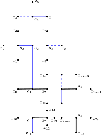
Figure 2. A tree-like molecular graph, where $x_{i}$’s denote external molecules and $a_{i}$’s denote internal molecules. The black double-line edges represent the diffusive edges in the black net, and the blue lines represent the diffusive or free edges in the blue net. Here, the dashed lines represent the redundant edges in the generalized doubly connected property.

Proof of Lemma 8.1.

With Lemmas 8.3 and 8.6, the proof of Lemma 8.1 uses the same argument as shown in Section 6 of [54]. Hence, we only give a sketch of the proof without presenting all the details.

By Lemma 8.3, to show (8.3), it suffices to prove that

$$\frac{1}{|\cal I|^{p}}\sum_{x_{i}\in\cal I:i=1,\ldots,p}\mathcal{G}_{\mathbf{x}}^{(\mu)}\prec\mathfrak{g}(K,\lambda,\eta)^{p-1}$$ (8.10)

for each deterministic graph $\mathcal{G}_{\mathbf{x}}^{(\mu)}$ satisfying (8.5) and properties (a)–(c) in Lemma 8.3. For this purpose, we first bound $\mathcal{G}_{\mathbf{x}}^{(\mu)}$ by a new graph where the coefficient is bounded by its absolute value, the ghost and free edges remain unchanged, and the remaining graph is bounded (in the sense of absolute value) as follows:

• For each molecule in $\mathcal{G}_{\mathbf{x}}^{(\mu)}$, we choose a representative vertex in it, called center of the molecule. For an external molecule containing an external vertex $x_{i}$, let $x_{i}$ be its center. If an external molecule contains multiple external vertices $x_{k_{1}},\ldots,x_{k_{r}}$, then we choose one of them as the center.

• We define a “pseudo-waved edge” between vertices $x$ and $y$ as a waved edge representing the factor $\mathcal{W}_{xy}:=W^{-d}\mathbf{1}({|x-y|\leq W(\log W)^{2}})$. Now, we bound the waved edges within molecules as follows. First, each waved edge between vertices $x$ and $y$ is bounded by a factor $\operatorname{O}(W^{-d}\mathbf{1}(|x-y|\leq W(\log W)^{1+\tau}))$ for a constant $\tau\in(0,1)$. By the definition of $S$ and the bound (3.11), this leads to an error of order $\operatorname{O}(W^{-D})$ for any large constant $D>0$. Second, suppose $x$ and $y$ belong to a molecule $\cal M$ with center $x_{0}$. We can further bound the factor $W^{-d}\mathbf{1}(|x-y|\leq W(\log W)^{1+\tau})$ by pseudo-waved edges between them and $x_{0}$, i.e., $W^{d}\cdot\mathcal{W}_{xx_{0}}\cdot\mathcal{W}_{yx_{0}}$. Finally, if there are multiple pseudo-wave edges between an atom $x$ and $x_{0}$, we only keep one of them, while the rest of them provide a power of $W$ that can be included into the coefficient.

• By (3.1), a diffusive edge between vertices $x$ and $y$ is bounded by a “pseudo-diffusive edge” that represents the factor $B_{xy}$. Suppose $x$ and $y$ belong to molecules $\cal M_{1}$ and $\cal M_{2}$ with centers $x_{0}$ and $y_{0}$ ($\cal M_{1}$ and $\cal M_{2}$ can be the same molecule). Then, up to an error of order $\operatorname{O}(W^{-D})$, we can further bound the $B_{xy}$ edge by

  $$(\log W)^{2d}B_{x_{0}y_{0}}\mathbf{1}(|x-x_{0}|\leq W(\log W)^{2})\mathbf{1}(|y-y_{0}|\leq W(\log W)^{2}).$$

  For a labeled diffusive edge $\mathring{\vartheta}_{xy}({\mathcal{E}})$ or $(\mathring{\vartheta}{\mathcal{E}}_{1}\mathring{\vartheta}{\mathcal{E}}_{2}\mathring{\vartheta}\cdots\mathring{\vartheta}{\mathcal{E}}_{k}\mathring{\vartheta})_{xy}$ as in (3.33), we can bound it in a similar manner. However, in the latter case, we multiply the coefficient of the graph by the extra factor $\prod_{i=1}^{k}\boldsymbol{\psi}({\mathcal{E}}_{i})$.

After the above operations, we can bound $\mathcal{G}_{\mathbf{x}}^{(\mu)}$ by a new deterministic graph:

$$\mathcal{G}_{\mathbf{x}}^{(\mu)}\prec(\log W)^{C}{\mathcal{G}}_{\mathbf{x}}^{\prime}+\operatorname{O}(W^{-D}).$$ (8.11)

Then, we sum over all internal vertices in ${\mathcal{G}}_{\mathbf{x}}^{\prime}$ that are not centers of molecules and get that:

$${\mathcal{G}}_{\mathbf{x}}^{\prime}\prec(\log W)^{C}c^{\prime\prime}(\mathcal{G}_{\mathbf{x}}^{(\mu)})\cdot{\mathcal{G}}_{\mathbf{x}}^{\prime\prime},$$ (8.12)

where $c^{\prime\prime}(\mathcal{G}_{\mathbf{x}}^{(\mu)})$ is a positive coefficient coming from the coefficient of $\mathcal{G}_{\mathbf{x}}^{(\mu)}$ and the above operations (1)–(3). ${\mathcal{G}}_{\mathbf{x}}^{\prime\prime}$ is a deterministic graph consisting of external vertices, internal vertices that are centers of internal molecules, pseudo-diffusive, free, or ghost edges between them, as well as potential pseudo-waved edges between external vertices. This graph satisfies (a)–(c) of Lemma 8.3. Moreover, if we define ${\mathsf{wsize}}({\mathcal{G}}_{\mathbf{x}}^{\prime\prime})$ as (note that we do not count the factors from the ghost edges as in (7.1))

$${\mathsf{wsize}}({\mathcal{G}}_{\mathbf{x}}^{\prime\prime})= \mathfrak{h}_{\lambda}^{\#\{\text{free edges}\}+\#\{\text{pseudo-diffusive edges}\}}W^{-d(\#\{\text{pseduo-waved edges}\}-\#\{\text{internal vertices}\})},$$

then it satisfies that

$$c^{\prime\prime}(\mathcal{G}_{\mathbf{x}}^{(\mu)}){\mathsf{wsize}}({\mathcal{G}}_{\mathbf{x}}^{\prime\prime})\prec{\mathsf{wsize}}(\mathcal{G}_{\mathbf{x}}^{(\mu)})\lesssim\mathfrak{h}_{\lambda}^{q-1}.$$

Next, we bound the summations over the internal vertices in ${\mathcal{G}}_{\mathbf{x}}^{\prime\prime}$. For this purpose, we introduce two new types of edges:

• a “silent diffusive edge” between vertices $x$ and $y$ represents a factor

  $$\widetilde{B}_{xy}:=\frac{\beta(\lambda)}{W^{4}\langle x-y\rangle^{d-4}};$$ (8.13)

• a “silent free edge” between vertices $x$ and $y$ represents a factor $\frac{1}{N\eta}\frac{L^{2}}{W^{2}}.$

Like free and ghost edges, a silent free edge is just a scalar and we introduce it to help with analyzing the structures of graphs. With the generalized doubly connected property of ${\mathcal{G}}_{\mathbf{x}}^{\prime\prime}$, we can choose a collection of blue trees such that every internal vertex connects to an external vertex through a unique path on a blue tree. These blue trees are disjoint, each of which contains an external vertex as the root. Then, we will sum over all internal vertices from leaves of the blue trees to the roots. In bounding every summation, we use the following two estimates with $k\geq 1$ and $r\geq 0$:

$$\begin{split}&\sum_{x}\prod_{j=1}^{k}B_{xy_{j}}\cdot\prod_{s=1}^{r}\widetilde{B}_{xz_{s}}\cdot B_{xa}\\ &\prec\beta(\lambda)\sum_{l=1}^{k}\prod_{j:j\neq l}B_{y_{j}y_{l}}\cdot\Big{(}\widetilde{B}_{y_{l}a}\prod_{s=1}^{r}\widetilde{B}_{z_{s}a}+\widetilde{B}_{y_{l}a}\prod_{s=1}^{r}\widetilde{B}_{z_{s}y_{l}}+\sum_{t=1}^{r}\widetilde{B}_{y_{l}z_{t}}\widetilde{B}_{z_{t}a}\prod_{s:s\neq t}\widetilde{B}_{z_{s}z_{t}}\Big{)},\end{split}$$ (8.14)

$$\sum_{x}\prod_{j=1}^{k}B_{xy_{j}}\cdot\prod_{s=1}^{r}\widetilde{B}_{xz_{s}}\prec\beta(\lambda)\frac{L^{2}}{W^{2}}\sum_{l=1}^{k}\prod_{j:j\neq l}B_{y_{j}y_{l}}\cdot\Big{(}\prod_{s=1}^{r}\widetilde{B}_{z_{s}y_{l}}+\sum_{t=1}^{r}\widetilde{B}_{y_{l}z_{t}}\prod_{s:s\neq t}\widetilde{B}_{z_{s}z_{t}}\Big{)}.$$ (8.15)

The LHS of (8.14) is a star graph consisting of $k$ pseudo-diffusive edges (where at least one of them is in the black tree), a pseudo-diffusive edge in the blue tree, and $r$ silent pseudo-diffusive edges connected with $x_{i}$, while every graph on the RHS is a connected graph consisting of $(k-1)$ pseudo-diffusive edges and $(r+1)$ silent pseudo-diffusive edges (together with an additional $\beta(\lambda)$ factor). The estimate (8.15) can be applied to the case where the blue edge is a ghost or free edge. (Of course, there may be multiple free edges connected with $x$, in which case we can still use (8.14) and (8.15) by multiplying some $(N\eta)^{-1}$ factors with them.) After applying (8.15), we either lose a ghost edge or change one free edge to a silent free edge (together with an additional $\beta(\lambda)$ factor).

Summing over all internal vertices in ${\mathcal{G}}_{\mathbf{x}}^{\prime\prime}$ from leaves of the blue trees to the roots and applying (8.14) and (8.15) to bound each summation, we obtain that

$$c^{\prime\prime}(\mathcal{G}_{\mathbf{x}}^{(\mu)}){\mathcal{G}}_{\mathbf{x}}^{\prime\prime}\prec\sum_{\gamma}c_{\gamma}\widetilde{\mathcal{G}}_{\mathbf{x}}^{(\gamma)}+\operatorname{O}(W^{-D})\,,$$ (8.16)

where the RHS is a sum of $\operatorname{O}(1)$ many deterministic graphs $\widetilde{\mathcal{G}}_{\mathbf{x}}^{(\gamma)}$ consisting of external vertices and pseudo-diffusive, silent diffusive, free, silent free, and pseudo-waved edges between them, and $c_{\gamma}$ denotes the coefficient. Moreover, these graphs and coefficients satisfy the following properties:

• Suppose that $t$ of the $q$ external vertices are centers of external molecules. Without loss of generality, assume that $x_{1},\ldots,x_{t}$ are these centers. Among these $t$ vertices, there are $k_{s}\geq\lceil t/2\rceil$ special vertices, each connected to a unique pseudo-diffusive/free edge. We call these $k_{s}$ pseudo-diffusive/free edges associated with the $k_{s}$ special vertices as special edges.

• We define ${\mathsf{wsize}}(\widetilde{\mathcal{G}}_{\mathbf{x}}^{(\gamma)})$ as

  $${\mathsf{wsize}}(\widetilde{\mathcal{G}}_{\mathbf{x}}^{(\gamma)})= \mathfrak{h}_{\lambda}^{Fr+SF+PD+SD}W^{-(q-t)d},$$ (8.17)

  where $Fr$, $SF$, $PD$, and $SD$ denote the numbers of free, silent free, pseudo-diffusive, and silent diffusive edges in $\widetilde{\mathcal{G}}_{\mathbf{x}}^{(\gamma)}$. Then, for every $\gamma$, we have that

  $$c_{\gamma}{\mathsf{wsize}}(\widetilde{\mathcal{G}}_{\mathbf{x}}^{(\gamma)})\lesssim c^{\prime\prime}(\mathcal{G}_{\mathbf{x}}^{(\mu)}){\mathsf{wsize}}({\mathcal{G}}_{\mathbf{x}}^{\prime\prime})\prec{\mathsf{wsize}}(\mathcal{G}_{\mathbf{x}}^{(\mu)})\lesssim\mathfrak{h}_{\lambda}^{q-1}.$$ (8.18)

The proof of (8.16) and these two conditions is similar to that in Section 6.1 of [54], so we omit the details.

Finally, we sum over the external vertices $x_{1},\ldots,x_{q}$ in $\widetilde{\mathcal{G}}_{\mathbf{x}}^{(\gamma)}$. For the $q-t$ external vertices $x_{t+1},\ldots,x_{q}$ that are not centers, their averages provide a $K^{-(q-t)d}$ factor. For the remaining $t$ vertices, each of them is connected with at least one silent/non-silent pseudo-diffusive or free edge. Thus, its average over $\cal I$ provides at least a factor

$$\frac{\beta(\lambda)}{W^{4}K^{d-4}}+\frac{1}{N\eta}\frac{L^{2}}{W^{2}}.$$ (8.19)

Furthermore, we will see that each average over an external vertex connected with a non-silent edge contributes a better factor

$$\frac{\beta(\lambda)}{W^{2}K^{d-2}}+\frac{1}{N\eta}+\frac{1}{K^{d/2}}\sqrt{\frac{\beta(\lambda)}{N\eta}\frac{L^{2}}{W^{2}}}.$$ (8.20)

By property (i) above, there are $k_{s}\geq\lceil t/2\rceil$ special external vertices, each associated with a unique special non-silent edge. Therefore, on average, each external vertex $x_{i}$, $i\in\llbracket{1,t}\rrbracket$, provides at least a factor $\mathfrak{g}(K,\lambda,\eta)$.

To rigorously justify the above argument, we estimate the averages over the special external vertices. We use the following two estimates to bound the average over such an external vertex $x$ connected with a special diffusive edge: for $k\geq 1$ and $r\geq 0$,

$$\frac{1}{|\cal I|}\sum_{x\in\cal I}B_{xy_{1}}^{2}\prod_{j=2}^{k}B_{xy_{j}}\cdot\prod_{s=1}^{r}\widetilde{B}_{xz_{s}}\prec\frac{\beta(\lambda)}{W^{d}}\frac{\beta(\lambda)}{K^{d}}\sum_{l=1}^{k}\sum_{t=1}^{r}\prod_{j\in\llbracket{k}\rrbracket\setminus\{l\}}B_{y_{j}y_{l}}\cdot\widetilde{B}_{y_{1}z_{t}}\cdot\prod_{s:s\neq t}\widetilde{B}_{z_{s}z_{t}},$$ (8.21)

$$\frac{1}{|\cal I|}\sum_{x\in\cal I}\prod_{j=1}^{k}B_{xy_{j}}\cdot\prod_{s=1}^{r}\widetilde{B}_{xz_{s}}\prec\frac{\beta(\lambda)}{W^{2}K^{d-2}}\sum_{l=1}^{k}\sum_{t=1}^{r}\prod_{j\in\llbracket{k}\rrbracket\setminus\{l\}}B_{y_{j}y_{l}}\cdot\widetilde{B}_{y_{l}z_{t}}\cdot\prod_{s:s\neq t}\widetilde{B}_{z_{s}z_{t}}.$$ (8.22)

Here, we only include the pseudo-diffusive and silent diffusive edges connected with $x$. If there are free or silent free edges connected with $x$, we can still use (8.21) and (8.22) by multiplying them with the corresponding factors. We apply the above two estimates in two different cases. In the first case, suppose the special diffusive edge associated with $x$ is paired with the special diffusive edge associated with $y_{1}$. Then, we use (8.21) to bound the average over $x$ by a factor $\beta(\lambda)^{2}W^{-d}K^{-d}$ times a sum of new graphs, each of which is still connected and has two fewer special vertices. If the first case does not happen, then we use (8.22) to bound the average over $x$ by a factor $\beta(\lambda)W^{-2}K^{-(d-2)}$ times a sum of new graphs, each of which is still connected and has one fewer special vertex.

Second, we sum over special external vertices connected with non-silent free edges. Given such an external atom $x$, we use (1) the trivial identity $|\cal I|^{-1}\sum_{x\in\cal I}1=1$ if $x$ is only connected to silent/non-silent free edges, (2) the estimate (8.22) if $x$ is connected to at least one pseudo-diffusive edge, or (3) the following estimate if $x$ is connected to silent diffusive edges but no pseudo-diffusive edges:

$$\frac{1}{|\cal I|}\sum_{x\in\cal I}\prod_{s=1}^{r}\widetilde{B}_{xz_{s}}\prec\frac{\beta(\lambda)}{W^{4}K^{d-4}}\sum_{t=1}^{r}\prod_{s:s\neq t}\widetilde{B}_{z_{s}z_{t}}.$$ (8.23)

In this way, we can bound the average over $x$ by a factor $(N\eta)^{-1}$ times a sum of new graphs, each of which is still connected and has one fewer special external vertex.

Third, after summing over all special external vertices, we then sum over the non-special external vertices one by one using $|\cal I|^{-1}\sum_{x\in\cal I}1=1$ or the estimate (8.23). Each summation yields at least a factor (8.19) times a sum of new connected graphs. Finally, the average over the last vertex is equal to $1$.

Overall, after summing over all external vertices $x_{1},\ldots,x_{t}$, we can obtain that

$$\frac{1}{|\cal I|^{q}}\sum_{x_{i}\in\cal I:i\in\llbracket{1,q}\rrbracket}\widetilde{\cal G}_{{\bf{x}}}^{(\gamma)} \prec\mathfrak{h}_{\lambda}^{(Fr+SF+PD+SD)-(t-1)}\left(\frac{1}{K^{d}}\right)^{q-t}\left(\frac{\beta(\lambda)}{K^{d}}\right)^{k_{1}}\left(\frac{\beta(\lambda)}{W^{2}K^{d-2}}+\frac{1}{N\eta}\right)^{k_{s}-2k_{1}}$$

$$\quad\times\left(\frac{\beta(\lambda)}{W^{4}K^{d-4}}+\frac{1}{N\eta}\frac{L^{2}}{W^{2}}\right)^{t-1-(k_{s}-k_{1})},$$ (8.24)

where $\lceil t/2\rceil\leq k_{s}\leq t-1$ is the number of special external vertices and $0\leq k_{1}\leq\lfloor k_{s}/2\rfloor$ is the number of times that (8.21) has been applied. Here, the first factor on the RHS comes from $(Fr+SF+PD+SD)-(t-1)$ silent/non-silent pseudo-diffusive and free edges that become self-loops during the summation (for example, the $\beta(\lambda)/W^{d}$ factor in (8.21) comes from a pseudo-diffusive edge that becomes a self-loop in the summation), all of which are bounded by $\mathfrak{h}_{\lambda}$. The factor $K^{-d(q-t)}$ results from averaging over the $q-t$ external vertices that are not centers of molecules. The third and fourth factors come from averages over special external vertices, while the last factor on the RHS is due to averages over the remaining non-special external vertices. Together with (8.17) and (8.18), this leads to

$$\frac{1}{|\cal I|^{p}}\sum_{x_{i}\in\cal I:i\in\llbracket{p}\rrbracket}c_{\gamma}\widetilde{\mathcal{G}}_{\mathbf{x}}^{(\gamma)} \prec\frac{1}{|\cal I|^{p-q}}\left(\frac{\beta(\lambda)}{K^{d}}\right)^{q-t+k_{1}}\left(\frac{\beta(\lambda)}{W^{2}K^{d-2}}+\frac{1}{N\eta}\right)^{k_{s}-2k_{1}}\left(\frac{\beta(\lambda)}{W^{4}K^{d-4}}+\frac{1}{N\eta}\frac{L^{2}}{W^{2}}\right)^{t-1-(k_{s}-k_{1})}$$

$$\prec\sum_{k\in\llbracket{p}\rrbracket}\sum_{\lceil p/2\rceil\leq k\leq p-1}\left(\frac{\beta(\lambda)}{W^{2}K^{d-2}}+\frac{1}{N\eta}+\frac{1}{K^{d/2}}\sqrt{\frac{\beta(\lambda)}{N\eta}\frac{L^{2}}{W^{2}}}\right)^{k}$$

$$\quad\times\left(\frac{\beta(\lambda)}{W^{4}K^{d-4}}+\frac{1}{N\eta}\frac{L^{2}}{W^{2}}\right)^{p-1-k}\prec\mathfrak{g}(K,\lambda,\eta)^{p-1}.$$

Plugging it into (8.16) and further into (8.11) and (8.12), we conclude (8.3) since $D$ is arbitrary. ∎

8.2. Proof of Lemma 8.6

In this subsection, we prove (8.5) by keeping track of the change of the weak scaling size of the graphs from the expansion process. We will assign a subset of solid edges, denoted by $E(\cal G)$, to each graph $\cal G$ from the expansion. Moreover, we will see that these subsets can be chosen in a way such that the following quantity always decreases during our expansion process:

$${\mathsf{wsize}}(\cal G)\cdot\mathfrak{h}_{\lambda}^{\frac{1}{2}|E(\cal G)|}.$$ (8.25)

For the initial graph $\cal G_{{\bf{x}},\mathbf{\Sigma}}$, we choose $E(\cal G_{{\bf{x}},\mathbf{\Sigma}})$ as a subset of edges between external vertices with two edges removed. Then, roughly speaking, the subset $E({\cal G})$ changes during the expansion process as follows: if an edge in $E(\cal G)$ is “pulled” in some sense, we remove it from $E(\cal G)$; in the $V$-expansion presented in Theorem 7.4, for some graphs in $\mathcal{A}_{x,{\mathfrak{b}}_{1}{\mathfrak{b}}_{2}}$ that satisfy the equality in (7.8), they contain a new solid edge within the molecule containing $x$, and we include this edge in the subset $E(\cal G)$. For the initial graph, we select $E(\cal G_{{\bf{x}},\mathbf{\Sigma}})$ to be a subset of $q-2$ of the $q$ solid edges, while for each deterministic graph, we trivially have $E(\cal G_{{\bf{x}}}^{(\mu)})=\emptyset$. This gives us the inequality

$${\mathsf{wsize}}(\cal G_{{\bf{x}}}^{(\mu)})\leq{\mathsf{wsize}}(\cal G_{{\bf{x}},\mathbf{\Sigma}})\cdot\mathfrak{h}_{\lambda}^{\frac{1}{2}|E(\cal G_{{\bf{x}},\mathbf{\Sigma}})|}\lesssim\mathfrak{h}_{\lambda}^{q-1}.$$ (8.26)

We remark that this argument is not completely rigorous—in the following proof, we will only consider the quantity (8.25) for locally standard graphs, where the solid edges form loops. In particular, we will not specify $E(\cal G_{{\bf{x}},\mathbf{\Sigma}})$ for the initial graph.

Remark 8.7.

Given a loop graph $\cal G$ with $q$ solid edges, we choose $E(\cal G)$ to be a subset of $q-2$ solid edges for the following reasons. When we continuously apply the first four terms on the RHS of (7.3) to each external vertex in the loop graph, every time we replace a pair of $G$ and $\overline{G}$ edges with a diffusive/free edge and a $G/\overline{G}$ edge, the size of the graph decreases by a factor $\mathfrak{h}_{\lambda}^{1/2}$. Consequently, after the first $(q-2)$ steps, the size of the graph decreases by $\mathfrak{h}_{\lambda}^{(q-2)/2}=\mathfrak{h}_{\lambda}^{|E(\cal G)|/2}$. For the last two edges, they can be paired and replaced by a single diffusive edge, in which case the size of the graph remains unchanged. The following illustration depicts this process for a loop graph with $q=6$ edges:

Due to this observation, in the following proof, for a locally standard graph $\cal G$, we will choose $E(\cal G)$ such that

each loop containing an edge in $$E(\cal G) E(\cal G)$$ must include at least 2 solid edges that are not in . (8.27)

We now look at the expansion process. We first consider the initial local expansion, where we expand the graph $\cal G_{{\bf{x}},\mathbf{\Sigma}}$ into a sum of $\operatorname{O}(1)$ many locally regular graphs (where all solid edges are between internal vertices), $Q$-graphs, and graphs with negligible weak scaling size. In each locally regular graph $\cal G$, we denote by $n_{a}$ the number of internal vertices, $n_{W}$ the number of waved edges, and $t\in\llbracket{1,q}\rrbracket$ the number of external molecules. Since two external vertices belong to the same molecule if and only if they are connected through waved edges, we can derive that

$$n_{W}-n_{a}=q-t.$$ (8.28)

Next, we can choose $(t-1)$ solid edges in $\cal G$ that form a spanning tree of the $t$ external molecules, and we denote the subset of these edges by $E_{0}(\cal G)$. We assume that these edges belong to $a$ loops of solid edges. Every such loop contains at least one solid edge that does not belong to $E_{0}(\cal G)$. Hence, we need to remove at most $a$ solid edges from $E_{0}(\cal G)$ to get $E(\cal G)$ so that property (8.27) holds. Suppose we remove $a_{0}\leq a$ edges from $E_{0}(\cal G)$. Then, using (8.28) and the fact that $\cal G$ contains at least $(t-1+a)$ solid edges, we obtain

$${\mathsf{wsize}}(\cal G)\cdot\mathfrak{h}_{\lambda}^{\frac{1}{2}|E(\cal G)|}\lesssim W^{-(q-t)d}\mathfrak{h}_{\lambda}^{\frac{1}{2}(t-1+a)}\cdot\mathfrak{h}_{\lambda}^{\frac{1}{2}(t-1-a_{0})}\leq\mathfrak{h}_{\lambda}^{q-1}.$$

Now, given a locally regular graph $\cal G$ from the expansions, suppose we have chosen $E(\cal G)$ such that ${\mathsf{wsize}}(\cal G)\cdot\mathfrak{h}_{\lambda}^{|E(\cal G)|/2}\lesssim\mathfrak{h}_{\lambda}^{q-1}$, and property (8.27) holds. Then, we need to expand one of the $T$-variables in $\cal G$ according to 8.5. Suppose this $T$-variable is $T_{{\mathfrak{a}},{\mathfrak{b}}_{1}{\mathfrak{b}}_{2}}$. Without loss of generality, assume that the $G$ and $\overline{G}$ edges (denoted by $e_{1}$ and $\overline{e}_{1}$) forming the $T$-variable do not belong to $E(\cal G)$. (Otherwise, we can find two solid edges $e_{2}$ and $e_{3}$ that do not belong to $E(\cal G)$ and lie in the loop containing $e_{1}$ and $\overline{e}_{1}$. In this case, we can remove $e_{1}$ and $\overline{e}_{1}$ from $E(\cal G)$ and substitute them with the edges $e_{2}$ and $e_{3}$.) We then apply the $V$-expansion in Theorem 7.4 to

$$\cal G=\sum_{{\mathfrak{a}},{\mathfrak{b}}_{1},{\mathfrak{b}}_{2}}T_{{\mathfrak{a}},{\mathfrak{b}}_{1}{\mathfrak{b}}_{2}}\Gamma({\mathfrak{a}},{\mathfrak{b}}_{1},{\mathfrak{b}}_{2})$$

by substituting the complete $T$-equation (7.3) into $T_{{\mathfrak{a}},{\mathfrak{b}}_{1}{\mathfrak{b}}_{2}}$. We divide the discussion into the following cases.

Case 1: If we have replaced $T_{{\mathfrak{a}},{\mathfrak{b}}_{1}{\mathfrak{b}}_{2}}$ by the first four terms on the RHS of (7.3), then in each new graph, say $\cal G_{new}$, we have a new diffusive or free edge between ${\mathfrak{a}}$ and the molecule $\cal M_{1}$ or $\cal M_{2}$, as well as a solid edge between between $\cal M_{1}$ and $\cal M_{2}$. Consequently, ${\mathsf{wsize}}(\cal G_{new})$ is smaller than ${\mathsf{wsize}}(\cal G)$ by at least $\mathfrak{h}_{\lambda}^{1/2}$. Moreover, the original loop (denoted by $\mathrm{L}_{1}$) of solid edges containing $e_{1}$ and $\overline{e}_{1}$ in $\cal G$ becomes a new loop (denoted by $\mathrm{L}_{new}$) in $\cal G_{new}$ with one fewer solid edge. We then remove one edge (if there is one) from $E(\cal G)$ that belongs to $\mathrm{L}_{new}$, while all the other edges in $E(G)$ remain in $E(\cal G_{new})$. This gives that

$${\mathsf{wsize}}(\cal G_{new})\mathfrak{h}_{\lambda}^{\frac{1}{2}|E(\cal G_{new})|}\lesssim{\mathsf{wsize}}(\cal G)\mathfrak{h}_{\lambda}^{\frac{1}{2}|E(\cal G)|}.$$ (8.29)

If we have replaced $T_{{\mathfrak{a}},{\mathfrak{b}}_{1}{\mathfrak{b}}_{2}}$ by the fifth term on the RHS of (7.3), then in each new graph $\cal G_{new}$, ${\mathsf{wsize}}(\cal G_{new})$ is smaller than ${\mathsf{wsize}}(\cal G)$ by at least $\beta(\lambda)\mathfrak{h}_{\lambda}^{2}$: $\beta(\lambda)$ comes from the summation of $x$ over $\widetilde{\vartheta}_{{\mathfrak{a}}x}$, while the factor $\mathfrak{h}_{\lambda}^{2}$ is due to the doubly connected property of $\cal D^{(\gamma)}_{x,{\mathfrak{b}}_{1}{\mathfrak{b}}_{2}}$. Furthermore, the loop $\mathrm{L}_{1}$ becomes a new loop $\mathrm{L}_{new}$ with two fewer solid edges. Then, we remove two edges (if there are two) from $E(\cal G)$ that belong to $\mathrm{L}_{new}$, while all the other edges in $E(G)$ remain in $E(\cal G_{new})$. This gives that

$${\mathsf{wsize}}(\cal G_{new})\mathfrak{h}_{\lambda}^{\frac{1}{2}|E(\cal G_{new})|}\lesssim\beta(\lambda)\mathfrak{h}_{\lambda}\cdot{\mathsf{wsize}}(\cal G)\mathfrak{h}_{\lambda}^{\frac{1}{2}|E(\cal G)|}\leq{\mathsf{wsize}}(\cal G)\mathfrak{h}_{\lambda}^{\frac{1}{2}|E(\cal G)|}.$$ (8.30)

Case 2: We consider the star graphs in (LABEL:eq_Vexp). We take the sum of star graphs (7.12) that correspond to a particular pairing $\cal P(E_{p},\overline{E}_{p})$:

$$\cal G_{new}=\sum_{{\mathfrak{a}},{\mathfrak{b}}_{1},{\mathfrak{b}}_{2}}\sum_{x}\widetilde{\vartheta}_{{\mathfrak{a}}x}\cal G_{p,\gamma}^{\star}(x,{\mathfrak{b}}_{1},{\mathfrak{b}}_{2}).$$

If an edge in $E(\cal G)$ is pulled in the star graph, then we remove it from $E(\cal G_{new})$; otherwise, we keep it. Using the sum zero property (7.15) and the estimate (7.16), the coefficient of $\cal G_{new}$ is of order

$$\mathrm{cof}(\cal G_{new})=\operatorname{O}(\eta+\beta(\lambda)^{-1})=\operatorname{O}(\beta(\lambda)^{-1}).$$

Thus, ${\mathsf{wsize}}(\cal G_{new})$ satisfies that

$${\mathsf{wsize}}(\cal G_{new})\lesssim\beta(\lambda)\cdot|\mathrm{cof}(\cal G_{new})|\mathfrak{h}_{\lambda}^{\frac{1}{2}(|E(\cal G)|-|E(\cal G_{new})|)}\cdot{\mathsf{wsize}}(\cal G)=\mathfrak{h}_{\lambda}^{\frac{1}{2}(|E(\cal G)|-|E(\cal G_{new})|)}\cdot{\mathsf{wsize}}(\cal G),$$

where $\beta(\lambda)$ comes from the summation of the diffusive edge $\widetilde{\vartheta}_{{\mathfrak{a}}x}$ over $x$, while the factor $\mathfrak{h}_{\lambda}^{\frac{1}{2}(|E(\cal G)|-|E(\cal G_{new})|)}$ accounts for the decrease in the weak scaling size due to the $(|E(\cal G)|-|E(\cal G_{new})|)$ edges that have been pulled in the star graphs. Finally, consider any edge $e$ in $\cal G_{new}$ and the loop containing it. Removing $e$ from the loop creates a path between the two endpoints of $e$. This path either traverses two edges that are not in $E(\cal G)$ or passes through the center molecule $\cal M_{x}$ through two edges that have been pulled in the star graphs. Thus, the property (8.27) still holds for $\cal G_{new}$.

Case 3: We consider the higher order graphs in $\sum_{x}\widetilde{\vartheta}_{{\mathfrak{a}}x}\mathcal{A}_{x,{\mathfrak{b}}_{1}{\mathfrak{b}}_{2}}$ from (LABEL:eq_Vexp), and they are not recollision graphs. Pick one of the graphs, denoted $\cal G_{new}$. Similar to Case 2, if an edge in $E(\cal G)$ is pulled in $\cal G_{new}$, then we remove it from $E(\cal G)$; otherwise, we keep it. This process results in a subset $E^{\prime}(\cal G_{new})$. If ${\mathsf{wsize}}(\cal G_{new})$ satisfies

$${\mathsf{wsize}}(\cal G_{new})\lesssim\beta(\lambda)\mathfrak{h}_{\lambda}\cdot{\mathsf{wsize}}(\cal G)\mathfrak{h}_{\lambda}^{\frac{1}{2}(|E(\cal G)|-|E^{\prime}(\cal G_{new})|)},$$ (8.31)

then we set $E(\cal G_{new})=E^{\prime}(\cal G_{new})$ and have that

$${\mathsf{wsize}}(\cal G_{new})\mathfrak{h}_{\lambda}^{\frac{1}{2}|E(\cal G_{new})|}\leq\beta(\lambda)\mathfrak{h}_{\lambda}\cdot{\mathsf{wsize}}(\cal G)\mathfrak{h}_{\lambda}^{\frac{1}{2}(|E(\cal G)|-|E(\cal G_{new})|)}\cdot\mathfrak{h}_{\lambda}^{\frac{1}{2}|E(\cal G_{new})|}\leq{\mathsf{wsize}}(\cal G)\mathfrak{h}_{\lambda}^{\frac{1}{2}|E(\cal G)|}.$$

If (8.31) does not hold, then we at least have

$${\mathsf{wsize}}(\cal G_{new})\lesssim\beta(\lambda)\mathfrak{h}_{\lambda}^{1/2}\cdot{\mathsf{wsize}}(\cal G)\mathfrak{h}_{\lambda}^{\frac{1}{2}(|E(\cal G)|-|E^{\prime}(\cal G_{new})|)}$$ (8.32)

by (7.8). This scenario can only occur when we replace $T_{{\mathfrak{a}},{\mathfrak{b}}_{1}{\mathfrak{b}}_{2}}$ by $\sum_{x}\widetilde{\vartheta}_{{\mathfrak{a}}x}\widetilde{\cal Q}_{x,{\mathfrak{b}}_{1}{\mathfrak{b}}_{2}}$, where $\widetilde{\cal Q}_{x,{\mathfrak{b}}_{1}{\mathfrak{b}}_{2}}$ denotes the sum of the $Q$-graphs in (4.23), because all other $Q$-graphs have ${\mathsf{wsize}}$ smaller than ${\mathsf{wsize}}(T_{{\mathfrak{a}},{\mathfrak{b}}_{1}{\mathfrak{b}}_{2}})$ by at least $\beta(\lambda)\mathfrak{h}_{\lambda}$. Furthermore, if $T_{{\mathfrak{a}},{\mathfrak{b}}_{1}{\mathfrak{b}}_{2}}$ is replaced by a $Q$-graph that is not included in (7.21), then after Step 1 of the $Q$-expansion, each resulting graph that does not satisfy (8.31) either has a light weight or an atom $x$ with non-neutral charge. In this case, we must perform at least one light weight expansion or a $GG$-expansion, which decreases the ${\mathsf{wsize}}$ of the graph by at least $\mathfrak{h}_{\lambda}^{1/2}$, ensuring that the resulting graphs still satisfy (8.31).

It remains to consider the $Q$-expansions involving the terms in (7.21). Since we are considering the non-recollision graphs, only the first two terms in (7.21) are relevant. Following the $Q$-expansion process, we observe that a non-recollision graph $\cal G_{new}$ that does not satisfy (8.31) must have one (and only one) of the following structures:

In other words, there is a new solid edge $e$ within the molecule $\cal M_{x}$ connecting the two pulled edges of an edge in $E(\cal G)$. We then add this edge to $E^{\prime}(\cal G_{new})$ and let $E(\cal G_{new})=E^{\prime}(\cal G_{new})\cup\{e\}$. With (8.32), we get

$${\mathsf{wsize}}(\cal G_{new})\mathfrak{h}_{\lambda}^{\frac{1}{2}|E(\cal G_{new})|}\leq\beta(\lambda)\mathfrak{h}_{\lambda}^{\frac{1}{2}}\cdot{\mathsf{wsize}}(\cal G)\mathfrak{h}_{\lambda}^{\frac{1}{2}(|E(\cal G)|-|E^{\prime}(\cal G_{new})|)}\cdot\mathfrak{h}_{\lambda}^{\frac{1}{2}|E(\cal G_{new})|}\leq{\mathsf{wsize}}(\cal G)\mathfrak{h}_{\lambda}^{\frac{1}{2}|E(\cal G)|}.$$

Finally, since recollisions between $\cal M_{x}$ and existing vertices in $\cal G$ do not occur, a similar argument as in Case 2 shows that (8.27) holds for $\cal G_{new}$ under such a choice of $E(\cal G_{new})$.

Case 4: Finally, we consider the recollision graphs in $\sum_{x}\widetilde{\vartheta}_{{\mathfrak{a}}x}\mathcal{R}_{x,{\mathfrak{b}}_{1}{\mathfrak{b}}_{2}}$ in (LABEL:eq_Vexp). Pick any graph $\cal G_{new}$ coming from the $Q$-expansion of a graph obtained by replacing $T_{{\mathfrak{a}},{\mathfrak{b}}_{1}{\mathfrak{b}}_{2}}$ with a $Q$-graph in (7.3). This $Q$-graph has ${\mathsf{wsize}}$ at most $\beta(\lambda){\mathsf{wsize}}(T_{{\mathfrak{a}},{\mathfrak{b}}_{1}{\mathfrak{b}}_{2}})$. Thus, the graph before the $Q$-expansions has ${\mathsf{wsize}}$ at most $\beta(\lambda){\mathsf{wsize}}(\cal G)$. We now check how the ${\mathsf{wsize}}$ of the graphs decreases with respect to the changes of $E(\cal G)$.

If an edge in $E(\cal G)$ is “pulled” during the expansion process leading to $\cal G_{new}$, then we remove it from $E(\cal G)$; otherwise, we keep it. This process results in the subset $E(\cal G_{new})$. Here, a “pulling” of a solid edge $e\in E(\cal G)$ refers to one of the following changes made to the edge:

• The edge becomes two edges due to the operations (6.22) and (6.25) in $Q$-expansions, or as a result of the partial derivatives $\partial_{\alpha\beta}$ in Gaussian integration by parts—these represent the “normal pulling” of the edge. In this case, the ${\mathsf{wsize}}$ of the graph decreases by at least $\mathfrak{h}_{\lambda}^{1/2}$, compensating for the loss of the edge $e$ from $E(\cal G)$ to $E(\cal G_{new})$.

• The edge is not pulled as in case (1), but at least one of its endpoints is merged with another vertex due to the dotted edge associated with a new solid edge produced in the expansions. Denote such an endpoint by vertex $a$. We know that $a$ is standard neutral because the graph $\cal G$ is locally regular. In particular, in $\cal G$, $a$ is attached with a waved edge, the edge $e$, and another edge, say $e^{\prime}$, which has an opposite charge compared to edge $e$. This scenario occurs only when the edge $e^{\prime}$ is pulled as in case (1) and we have replaced the new solid edge, say $e^{\prime\prime}$, attached to $a$ by a dotted edge with coefficient $m(z)$ or $\overline{m}(z)$. We draw the following pictures to illustrate this process:

  

  Here, we did not indicate the directions of the solid edges, and we have taken $e$ to be a blue solid edge without loss of generality. From the first graph to the second, the edge $e^{\prime}$ is pulled to a vertex $b$; from the second graph to the third, we have replaced the edge $e^{\prime\prime}$ by a dotted edge with a coefficient $\overline{m}(z)$ and merged the two vertices $a$ and $b$. After merging $a$ with $b$, we lose one internal vertex and one solid edge, resulting in a decrease in the ${\mathsf{wsize}}$ by $W^{-d}\mathfrak{h}_{\lambda}^{-1/2}\asymp\beta(\lambda)^{-1}\mathfrak{h}_{\lambda}^{1/2}$. The $\mathfrak{h}_{\lambda}^{1/2}$ factor compensates for the loss of the edge $e$ from $E(\cal G)$ to $E(\cal G_{new})$, and we get an additional $\beta(\lambda)^{-1}$ factor.

• One solid edge (denoted by $e^{\prime}$) attached to an endpoint (denoted by $a$) of the edge $e$ becomes an $S^{\pm}$ edge. This change is a result of the second term in the $GG$-expansion (6.17). In this operation, we lose one solid edge while gaining an $S^{\pm}$ edge. Consequently, similar to case (2), the ${\mathsf{wsize}}$ of the graph decreases by $\beta(\lambda)^{-1}\mathfrak{h}_{\lambda}^{1/2}$, where the $\mathfrak{h}_{\lambda}^{1/2}$ factor compensates for the loss of the edge $e$ from $E(\cal G)$ to $E(\cal G_{new})$, and we get an additional $\beta(\lambda)^{-1}$ factor.

In sum, we see that if an edge in $E(G)$ has been “pulled” according to the three cases described above, the ${\mathsf{wsize}}$ of the resulting graph decreases by at least $\mathfrak{h}_{\lambda}^{1/2}$. Furthermore, if case (2) or (3) occurs at least once, we gain an extra factor $\beta(\lambda)^{-1}$. Even if cases (2) and (3) do not occur for the edges in $E(\cal G)$, they must have occurred for some edges in $\cal G$ that do not belong to $E(\cal G)$, since $\cal G_{new}$ is a recollision graph. Thus, we always get an additional $\beta(\lambda)^{-1}$ factor, leading to the conclusion that

$${\mathsf{wsize}}(\cal G_{new})\mathfrak{h}_{\lambda}^{\frac{1}{2}|E(\cal G_{new})|}\leq\beta(\lambda)\cdot\beta(\lambda)^{-1}\cdot{\mathsf{wsize}}(\cal G)\mathfrak{h}_{\lambda}^{\frac{1}{2}(|E(\cal G)|-|E(\cal G_{new})|)}\cdot\mathfrak{h}_{\lambda}^{\frac{1}{2}|E(\cal G_{new})|}={\mathsf{wsize}}(\cal G)\mathfrak{h}_{\lambda}^{\frac{1}{2}|E(\cal G)|}.$$

Finally, consider any edge $e$ in $\cal G_{new}$ and the loop containing it. In $\cal G_{new}$, one of the following cases occurs:

• The loop remains untouched during the expansions and retains its original structure.

• The loop contains at least two pulled edges, which do not belong to $E(\cal G_{new})$.

Thus, the property (8.27) remains valid for $\cal G_{new}$.

Applying the expansion strategy, 8.5, repeatedly, we finally get a sum of $\operatorname{O}(1)$ many deterministic graphs $\cal G_{{\bf{x}}}^{(\mu)}$ through a sequence of $V$-expansions. From the above discussions, we see that the quantity (8.25) always decreases in our expansions for carefully chosen subsets of edges $E(\cal G)$. Hence, (8.26) holds, which concludes the proof of (8.5).

8.3. Proof of Theorem 2.4

Denote $\mathcal{A}:=\operatorname{{\mathrm{Im}}}G=(G-G^{*})/(2\mathrm{i})$. We observe that the quantity of interest $\sum_{x\in I_{N}}(N|u_{\alpha}(x)|^{2}-1)$ can be controlled by $\operatorname{Tr}(\mathcal{A}\Pi\mathcal{A}\Pi)$, where $\Pi$ is a diagonal matrix with diagonal entries

$$\Pi_{xx}=(N/|I_{N}|)\mathbf{1}_{x\in I_{N}}-1.$$ (8.33)

The next lemma follows immediately from the spectral decomposition of $\cal A$.

Lemma 8.8 (Lemma 4.15 of [54]).

Let $z=E+\mathrm{i}\eta$ and $\Pi=\mathrm{diag}((\Pi_{x})_{x\in\mathbb{Z}^{d}_{L}})$ be an arbitrary real diagonal matrix. Then, for any $l\geq\eta$,

$${\sum_{\alpha,\beta:|\lambda_{\alpha}-E|\leq l,|\lambda_{\beta}-E|\leq l}}|\left\langle\mathbf{u}_{\alpha},\Pi\mathbf{u}_{\beta}\right\rangle|^{2}\leq\frac{4l^{4}}{\eta^{2}}\operatorname{Tr}\left[\mathcal{A}(z)\Pi\mathcal{A}(z)\Pi\right].$$ (8.34)

Note the matrix $\Pi$ defined through (8.33) has $\operatorname{Tr}\Pi=0$. Then, Theorem 2.4 follows from the next lemma on high-moment bounds of $\operatorname{Tr}\left(\mathcal{A}\Pi\mathcal{A}\Pi\right)$.

Lemma 8.9.

In the setting of Theorem 2.4, fix any $z=E+\mathrm{i}\eta$ with $|E|\leq 2-\kappa$ and $W^{\mathfrak{d}}\eta_{*}\leq\eta\leq 1$. Consider an arbitrary real diagonal matrix $\Pi$ such that $\operatorname{Tr}{\Pi}=0$ and $\Pi_{xx}$ is constant on each block, i.e., $\Pi_{xx}=\Pi_{yy}$ if $[x]=[y]$. Then, for any fixed $p\in\mathbb{N}$, we have that

$$\mathbb{E}\left[|\operatorname{Tr}\left[\mathcal{A}(z)\Pi\mathcal{A}(z)\Pi\right]|^{2p}\right]\prec\Big{(}\sum_{y}|\Pi_{yy}|\Big{)}^{2p}\Big{(}\max_{x}\sum_{y}B_{xy}|\Pi_{yy}|\Big{)}^{2p}\,.$$ (8.35)

Proof of Theorem 2.4.

For $\Pi$ defined in (8.33), we have $\operatorname{Tr}{\Pi}=0$, $\Pi_{xx}$ is constant on each block, and

$$\begin{split}\left|\left\langle\mathbf{u}_{\alpha},\Pi\mathbf{u}_{\alpha}\right\rangle\right|^{2}&=\Big{(}\sum_{x}\Pi_{xx}|u_{\alpha}(x)|^{2}\Big{)}^{2}=\bigg{(}\frac{1}{|I_{N}|}\sum_{x\in I_{N}}(N|u_{\alpha}(x)|^{2}-1)\bigg{)}^{2}\,.\end{split}$$ (8.36)

Next, taking $z=E+\mathrm{i}\eta$ with $\eta=N^{\mathfrak{d}}\eta_{*}$ and applying Markov’s inequality to (8.35), we obtain that

$$\operatorname{Tr}\left[\mathcal{A}(z)\Pi\mathcal{A}(z)\Pi\right] \prec\beta(\lambda)N\bigg{(}\frac{|I_{N}|^{2/d}}{W^{2}}\frac{N}{|I_{N}|}+\frac{L^{2}}{W^{2}}\bigg{)}\lesssim\frac{\beta(\lambda)N^{2}}{W^{2}|I_{N}|^{1-2/d}}\,.$$

Therefore, it follows from (8.34) that

$$\sup_{\alpha:|\lambda_{\alpha}-E|\leq\eta}|\left\langle\mathbf{u}_{\alpha},\Pi\mathbf{u}_{\alpha}\right\rangle|^{2} \prec\eta^{2}\operatorname{Tr}(\mathcal{A}\Pi\mathcal{A}\Pi)\prec\frac{\beta(\lambda)(N\eta)^{2}}{W^{2}|I_{N}|^{1-2/d}}\lesssim\frac{L^{10}W^{2d-12+2{\mathfrak{d}}}}{\beta(\lambda)|I_{N}|^{1-2/d}}\,,$$ (8.37)

$$\frac{1}{N\eta}\sum_{\alpha:|\lambda_{\alpha}-E|\leq\eta}|\left\langle\mathbf{u}_{\alpha},\Pi\mathbf{u}_{\alpha}\right\rangle|^{2} \prec\frac{\eta}{N}\operatorname{Tr}(\mathcal{A}\Pi\mathcal{A}\Pi)\prec\frac{\beta(\lambda)N\eta}{W^{2}|I_{N}|^{1-2/d}}\lesssim\frac{L^{5}W^{d-7+{\mathfrak{d}}}}{|I_{N}|^{1-2/d}}\,.$$ (8.38)

Combining (8.37) and (8.36), under condition (2.16), we conclude (2.17) since ${\mathfrak{d}}$ can be arbitrarily small. Moreover, from (8.38), we obtain that

$$\frac{1}{N}\sum_{\alpha:|\lambda_{\alpha}|\leq 2-\kappa}|\left\langle\mathbf{u}_{\alpha},\Pi\mathbf{u}_{\alpha}\right\rangle|^{2}\prec\frac{L^{5}W^{d-7+{\mathfrak{d}}}}{|I_{N}|^{1-2/d}}\,,$$

which, together with Markov’s inequality, implies that

$$\frac{1}{N}\,\left|\left\{\alpha:|\lambda_{\alpha}|\leq 2-\kappa,|\left\langle\mathbf{u}_{\alpha},\Pi\mathbf{u}_{\alpha}\right\rangle|\geq\epsilon\right\}\right|\prec\frac{\epsilon^{-2}L^{5}W^{d-7+{\mathfrak{d}}}}{|I_{N}|^{1-2/d}}.$$ (8.39)

Combining this bound with (8.36), with a union bound over $I_{N}\in\mathcal{I}$, we conclude (2.19) under (2.18). ∎

For the proof of Lemma 8.9, note that $|\operatorname{Tr}(\mathcal{A}\Pi\mathcal{A}\Pi)|^{2p}$ is a sum of expressions of the form

$$\sum_{\mathbf{s}}c(\mathbf{s})\sum_{\mathbf{x},\mathbf{y}}\mathcal{G}_{\mathbf{x},\mathbf{y}}^{\mathbf{s}}\prod_{i=1}^{2p}\Pi_{x_{i}x_{i}}\Pi_{y_{i}y_{i}},$$ (8.40)

where $\mathbf{s}=(s_{1},\ldots,s_{4p})\in\{\emptyset,{\dagger}\}^{4p}$, $c(\{s_{i}\})$ denotes a deterministic coefficient of order $\operatorname{O}(1)$, and $\mathcal{G}_{\mathbf{x},\mathbf{y}}$ are graphs of the form

$$\mathcal{G}^{\mathbf{s}}_{\mathbf{x},\mathbf{y}}=\prod_{i=1}^{2p}G^{(s_{2i-1})}_{x_{i}y_{i}}G^{(s_{2i})}_{y_{i}x_{i}}.$$ (8.41)

Now, to show (8.35), it suffices to prove the following counterpart of Lemmas 8.3 and 8.6 for $\mathbb{E}\mathcal{G}^{\mathbf{s}}_{\mathbf{x},\mathbf{y}}$, where the loop graph $\cal G_{\mathbf{x}}$ is replaced by a graph $\mathcal{G}^{\mathbf{s}}_{\mathbf{x},\mathbf{y}}$ with $2p$ connected components.

Lemma 8.10.

Suppose the setting of Lemma 8.3 holds. For the graph in (8.41), let $\Sigma_{1},\ldots,\Sigma_{q}$ be disjoint subsets that form a partition of the set of vertices $\{x_{1},\ldots,x_{2p},y_{1},\ldots,y_{2p}\}$ with $1\leq q\leq 4p$. We identify the indices in $\Sigma_{i}$, $i\in\llbracket{1,q}\rrbracket$, and denote the resulting graph by $\mathcal{G}^{\mathbf{s}}_{\mathbf{w},\mathbf{\Sigma}}(z)$, where $\mathbf{\Sigma}=(\Sigma_{1},\ldots,\Sigma_{q})$ and we denote the external vertices by ${\bf{w}}=(w_{1},\ldots,w_{q})$. Then, for any constant $D>0$, we have that

$$\mathbb{E}[\mathcal{G}^{\mathbf{s}}_{\mathbf{w},\mathbf{\Sigma}}]=\sum_{\mu}\mathcal{G}_{\mathbf{w}}^{(\mu)}+\operatorname{O}(W^{-D})\,,$$ (8.42)

where the RHS is a sum of $\operatorname{O}(1)$ many deterministic normal graphs $\mathcal{G}_{\mathbf{w}}^{(\mu)}$ with internal vertices and without silent edges such that the following properties hold.

• $\mathcal{G}_{\mathbf{w}}^{(\mu)}$ satisfies the properties (a) and (b) in Lemma 8.3 for $\mathcal{G}_{\mathbf{x}}^{(\mu)}$.

• If $w_{i}$ and $w_{j}$ are connected in $\mathcal{G}^{\mathbf{s}}_{\mathbf{w},\mathbf{\Sigma}}(z)$, then they are also connected in $\mathcal{G}_{\mathbf{w}}^{(\mu)}$ through non-ghost edges.

• The weak scaling size of $\mathcal{G}_{\mathbf{w}}^{(\mu)}$ satisfies that

  $${\mathsf{wsize}}(\mathcal{G}_{\mathbf{w}}^{(\mu)})\lesssim\mathfrak{h}_{\lambda}^{q-t},$$ (8.43)

  where $t$ denotes the number of connected components in $\mathcal{G}_{\mathbf{w}}^{(\mu)}$.

Proof.

The proof of this lemma follows the same approach as that for Lemma 8.3: we will expand the graph $\mathcal{G}^{\mathbf{s}}_{\mathbf{w},\mathbf{\Sigma}}$ by applying 8.5 repeatedly. Then, the resulting deterministic graphs $\mathcal{G}_{\mathbf{w}}^{(\mu)}$ will satisfy the above properties (a) and (b) due to Lemma 6.2 (a)–(c) in [54]. The weak scaling size condition (8.43) can be proved in the same way as Lemma 8.6. In fact, the proof of Lemma 8.6 demonstrates that the weak scaling size of each connected component in $\mathcal{G}_{\mathbf{w}}^{(\mu)}$ with $k$ external vertices can be bounded by $\operatorname{O}(\mathfrak{h}_{\lambda}^{k-1})$. Thus, the total weak scaling size of $\mathcal{G}_{\mathbf{w}}^{(\mu)}$ is at most $\operatorname{O}(\mathfrak{h}_{\lambda}^{q-t})$. We omit the details of the proof. ∎

Finally, we outline the proof of Lemma 8.9 by using Lemma 8.10.

Proof of Lemma 8.9.

Under the assumptions of Theorem 2.4, we know that the local law (8.1) holds by Theorem 2.2. Moreover, in the proof of Theorem 2.2, we have constructed a sequence of $T$-expansions up to arbitrarily high order ${\mathfrak{C}}$ by Theorem 4.9. We can choose ${\mathfrak{C}}$ large enough so that (5.3) holds. Then, we have a complete $T$-expansion by Lemma 7.2. Hence, the setting of Lemma 8.10 is satisfied, which gives the expansion (8.42). It remains to prove that

$$\sum^{\star}_{w_{1},\ldots,w_{q}\in\mathbb{Z}_{L}^{d}}\mathcal{G}_{\mathbf{w}}^{(\mu)}\mathbf{1}(\Sigma_{i}=w_{i}:i=1,\ldots,q)\prod_{i=1}^{2p}\Pi_{x_{i}x_{i}}\Pi_{y_{i}y_{i}}\prec\Big{(}\sum_{y}|\Pi_{yy}|\Big{)}^{2p}\Big{(}\max_{x}\sum_{y}B_{xy}|\Pi_{yy}|\Big{)}^{2p},$$ (8.44)

where recall that $\sum^{\star}$ means summation subject to the condition that $w_{1},\ldots,w_{q}$ all take distinct values:

$$\sum^{\star}_{w_{1},\ldots,w_{q}}=\sum_{w_{1},\ldots,w_{q}}\prod_{i\neq j\in\llbracket{q}\rrbracket}\mathbf{1}(w_{i}\neq w_{j}).$$

We can further remove the $\star$ from the LHS of (8.44) by expanding each $\times$-dotted edge as $\mathbf{1}(w_{i}\neq w_{j})=1-\mathbf{1}(w_{i}=w_{j})$. Taking the product of all these decompositions, we can write the graph as a linear combination of new graphs containing dotted edges. Then, in each new graph, we merge the vertices connected through dotted edges and rename them as $w_{1},\ldots,w_{\ell}$, where $1\leq\ell\leq q$ denotes the number of external vertices in the graph. In this way, we can rewrite the LHS of (8.44) as

$$\sum_{\ell=1}^{q}\sum_{\gamma}\sum_{\mathbf{w}=(w_{1},\ldots,w_{\ell})\in(\mathbb{Z}_{L}^{d})^{\ell}}\widetilde{\mathcal{G}}_{\mathbf{w}}^{(\gamma)}\mathbf{1}(\widetilde{\Sigma}_{i}=w_{i}:i=1,\ldots,\ell)\prod_{i=1}^{2p}\Pi_{x_{i}x_{i}}\Pi_{y_{i}y_{i}},$$

where $\gamma$ labels the new graphs $\widetilde{\mathcal{G}}_{\mathbf{w}}^{(\gamma)}$ and $\widetilde{\Sigma}_{i}$, $i\in\llbracket{\ell}\rrbracket$, denote the new partitions. Thus, to prove (8.44), it suffices to show that

$$\sum_{w_{1},\ldots,w_{\ell}\in\mathbb{Z}_{L}^{d}}\widetilde{\mathcal{G}}_{\mathbf{w}}^{(\gamma)}\mathbf{1}(\widetilde{\Sigma}_{i}=w_{i}:i=1,\ldots,\ell)\prod_{i=1}^{2p}\Pi_{x_{i}x_{i}}\Pi_{y_{i}y_{i}}\prec\Big{(}\sum_{y}|\Pi_{yy}|\Big{)}^{2p}\Big{(}\max_{x}\sum_{y}B_{xy}|\Pi_{yy}|\Big{)}^{2p}.$$ (8.45)

Note these new graphs $\widetilde{\mathcal{G}}_{\mathbf{w}}^{(\gamma)}$ also satisfy the properties (a)–(c) in Lemma 8.10 for $\mathcal{G}_{\mathbf{w}}^{(\mu)}$. Here, the condition (8.43) should become

$${\mathsf{wsize}}(\widetilde{\mathcal{G}}_{\mathbf{w}}^{(\gamma)})\lesssim\mathfrak{h}_{\lambda}^{\ell-t^{\prime}},$$ (8.46)

where $t^{\prime}$ denotes the number of connected components in $\widetilde{\mathcal{G}}_{\mathbf{w}}^{(\gamma)}$. To understand why (8.46) holds, we observe that whenever the count of connected components decreases by 1, it indicates the merging of external vertices connected by dotted edges, resulting in a reduction of external vertices by at least 1.

Next, a key observation is that it suffices to consider $\widetilde{\mathcal{G}}_{\mathbf{w}}^{(\gamma)}$ in which

$$\text{none of the $\ell$ external vertices is isolated if we do not include free edges into the edge set}.$$ (8.47)

Otherwise, suppose the external vertex $w_{1}$ is isolated without loss of generality. Since both our graphs and the matrix $\Pi$ are translation invariant on the block level, we know that $\sum_{w_{1}\in[x]}\widetilde{\mathcal{G}}_{\mathbf{w}}^{(\gamma)}$ does not depend on $[x]\in\widetilde{\mathbb{Z}}_{n}^{d}$, which implies that

$$\sum_{w_{1}}\widetilde{\mathcal{G}}_{\mathbf{w}}^{(\gamma)}\Pi_{w_{1}w_{1}}=W^{-d}\sum_{w_{1}\in[0]}\widetilde{\mathcal{G}}_{\mathbf{w}}^{(\gamma)}\cdot\sum_{w_{1}}\Pi_{w_{1}w_{1}}=0.$$

We remark that this is the only place where the zero trace condition for $\Pi$ is used.

It remains to prove that (8.45) holds for graphs $\widetilde{\mathcal{G}}_{\mathbf{w}}^{(\gamma)}$ that satisfy properties (a)–(c) in Lemma 8.10 and condition (8.47). This proof can be completed using the arguments from the proof of Lemma 3.4 in [54], followed by those in the proof of Proposition 4.16 in the same work. Since those proofs apply verbatim to our case, we omit the details here. This concludes (8.45) and hence completes the proof of Lemma 8.9. ∎

9. Sum zero property for self-energies

In this section, we present the proof of Proposition 6.3. It remains to give a construction of ${\mathcal{E}}_{k_{0}+1}$ and prove that it satisfies the sum zero property (3.29) and the properties (6.4)–(6.8). Following the ideas developed in [55], our proof is based on a comparison between the pseudo-self-energy $\widetilde{\mathcal{E}}_{k_{0}+1}$ and its infinite space limit.

Lemma 9.1.

In the setting of Proposition 6.3, fix any $z=E+\mathrm{i}\eta$ with $|E|\leq 2-\kappa$ and $\eta_{0}\leq\eta\leq 1$. Any deterministic doubly connected graph $\cal G\equiv\cal G(m(z),S,S^{\pm}(z),\vartheta(z),\{{\mathcal{E}}_{k}\}_{k=1}^{k_{0}}(z))$ in $\widetilde{\mathcal{E}}_{k_{0}+1}$ satisfies that

$$\left|{\cal G}_{xy}(z,W,L)-\cal G_{xy}^{\infty}(E,W,\infty)\right|\prec\left(\eta+t_{Th}^{-1}\right)\frac{\boldsymbol{\psi}(\cal G)}{\langle x-y\rangle^{d}},\quad\forall\ x,y\in\mathbb{Z}_{L}^{d},$$ (9.1)

$$\sum_{x\in\mathbb{Z}_{L}^{d}}\cal G_{xy}(z,W,L)-\sum_{x\in\mathbb{Z}^{d}}\cal G^{\infty}_{xy}(E,W,\infty)\prec\boldsymbol{\psi}(\cal G)\left(\eta+t_{Th}^{-1}\right),\quad\forall\ y\in[0].$$ (9.2)

Proof.

The proof of Lemma 9.1 is similar to those of [55, Lemma 7.7] and [54, Lemmas 5.5 and 5.6]. It relies on the estimates (3.17) and (3.19), Lemma 3.25, the induction assumption (6.8), and the fact that $\cal G$ is doubly connected, with each diffusive edge being redundant. Moreover, some arguments in the proof have also been revealed in the proof of Lemma 3.26. Hence, we omit the details of the proof. ∎

By studying the infinite space limit of $\widetilde{\mathcal{E}}_{k_{0}+1}$, the next lemma gives a construction of ${\mathcal{E}}_{k_{0}+1}^{\infty}(E,W,\infty)$, which in turn leads to a construction of ${\mathcal{E}}_{k_{0}+1}(z,W,L)$.

Lemma 9.2.

In the setting of Proposition 6.3, fix any $z=E+\mathrm{i}\eta$ with $|E|\leq 2-\kappa$ and $\eta_{0}\leq\eta\leq 1$. Then, any deterministic doubly connected graph $\widetilde{\cal G}(z,W,L)$ in $\widetilde{\mathcal{E}}_{k_{0}+1}$ can be expanded as

$$\widetilde{\cal G}(z,W,L)=\cal G(z,W,L)+\delta\cal G(z,W,L),$$ (9.3)

such that the following properties hold.

• The infinite space limit $\cal G^{\infty}(E,W,\infty)$ can be written as

  $$\cal G^{\infty}(E,W,\infty)=\frac{\boldsymbol{\psi}(\widetilde{\cal G})}{\beta(\lambda)}\left(\cal A_{\cal G}\otimes\mathbf{E}\right),$$ (9.4)

  where $\cal A_{\cal G}:\ell^{2}(\widetilde{\mathbb{Z}}^{d})\to\ell^{2}(\widetilde{\mathbb{Z}}^{d})$ is a fixed operator that does not depend on $W$ and satisfies the properties (6.5) and (6.6). Moreover, $\cal G-\cal G^{\infty}$ satisfies that

  $$\left|({\cal G}(z,W,L))_{xy}-({\cal G}^{\infty}(E,W,\infty))_{xy}\right|\prec\left(\eta+t_{Th}^{-1}\right)\frac{\boldsymbol{\psi}(\cal G)}{\langle x-y\rangle^{d}},\quad\forall\ x,y\in\mathbb{Z}_{L}^{d}.$$ (9.5)

• We have

  $$\boldsymbol{\psi}(\delta\cal G)=\beta(\lambda)W^{d}{\mathsf{size}}(\delta\cal G)\lesssim\lambda^{2}\boldsymbol{\psi}(\cal G).$$ (9.6)

Proof.

The graph $\cal G$ consists of $m\equiv m(z,\lambda)$ and the entries of the following matrices:

$$S,\quad S^{\pm},\quad\mathring{\vartheta},\quad\text{and}\quad\{{\mathcal{E}}_{k}\}_{k=1}^{k_{0}}.$$

Recall that $S,$ $S^{\pm}$, and $\mathring{\vartheta}$ can be written as in (6.39), where $S_{{L\to n}}$ is a tridiagonal matrix with $(S_{{L\to n}})_{[x][y]}=\delta_{[x][y]}+\lambda^{2}\mathbf{1}_{[x]\sim[y]}$, $S^{+}_{{L\to n}}=(1-m^{2}S_{{L\to n}})^{-1},$ and $\mathring{\vartheta}_{{L\to n}}$ can be expressed as

$$(\mathring{\vartheta}_{{L\to n}})_{[x][y]}=\frac{1}{1-|m|^{2}S_{{L\to n}}}-\frac{1}{n(1-|m|^{2})}.$$

Then, as $L\to\infty$ and $\eta\to 0$, $m(z)$ converges to

$$m(E)={\big{(}1+2d\lambda^{2}\big{)}^{-1/2}}m_{sc}\big{(}{E}/\sqrt{1+2d\lambda^{2}}\big{)}=m_{sc}(E)+\operatorname{O}(\lambda^{2}),$$

and the matrices $S$, $S^{+}$, and $\mathring{\vartheta}$ on $\mathbb{Z}_{L}^{d}$ converges to the following operators on $\mathbb{Z}^{d}$:

$$S_{\infty\to\infty}\otimes\mathbf{E},\quad S^{+}_{{\infty\to\infty}}\otimes\mathbf{E},\quad\vartheta_{{\infty\to\infty}}\otimes\mathbf{E}.$$

Here, $S_{\infty\to\infty}$, $\mathring{\vartheta}_{{\infty\to\infty}}$, and $S^{+}_{{\infty\to\infty}}$ define the following operators on $\widetilde{\mathbb{Z}}^{d}$:

$$\begin{split}&S_{{\infty\to\infty}}=(1+2d\lambda^{2})I-\lambda^{2}\widetilde{\Delta},\quad\vartheta_{{\infty\to\infty}}=\frac{1+2d\lambda^{2}}{\lambda^{2}}{\widetilde{\Delta}}^{\mathrm{inv}},\\ &S^{+}_{{\infty\to\infty}}=\left(1-m(E)^{2}S_{{\infty\to\infty}}\right)^{-1}=\left[1-m_{sc}(E)^{2}\right]^{-1}\left(1+\delta S^{+}_{\infty\to\infty}\right),\end{split}$$ (9.7)

where we used $|m_{sc}(E)|=1$ for every $E\in[-2,2]$, $\widetilde{\Delta}$ denotes the Laplacian operator on $\widetilde{\mathbb{Z}}^{d}$:

$$\Delta_{[x][y]}=2d\delta_{[x][y]}-\lambda^{2}\mathbf{1}_{[x]\sim[y]},$$

“$\mathrm{inv}$” stands for the pseudo-inverse, and the operator $\delta S^{+}_{\infty\to\infty}$ is defined as

$$\delta S^{+}_{\infty\to\infty}:=\left[m_{sc}(E_{\lambda})^{2}-m_{sc}(E)^{2}-m_{sc}(E_{\lambda})^{2}\frac{\lambda^{2}\widetilde{\Delta}}{1+2d\lambda^{2}}\right]\cdot S^{+}_{\infty\to\infty},\quad E_{\lambda}:={E}/\sqrt{1+2d\lambda^{2}}.$$

Finally, recall that the infinite space limit of ${\mathcal{E}}_{k}$, $k\in\llbracket{k_{0}}\rrbracket$, can be expressed as (6.4).

Due to the above observations, given $\widetilde{\cal G}^{\infty}$ written as $\widetilde{\cal G}^{\infty}=\cal B_{\widetilde{\cal G}}\otimes\mathbf{E}$ for some operator $\cal B_{\widetilde{\cal G}}$ on $\widetilde{\mathbb{Z}}^{d}$, we construct $\cal B_{\cal G}\otimes\mathbf{E}$ as follows, where $\cal B_{\cal G}$ is another operator defined on $\widetilde{\mathbb{Z}}^{d}$:

• Replace each $S_{\infty\to\infty}$ in $\cal B_{\widetilde{\cal G}}$ by $I$.

• Replace each $\vartheta_{\infty\to\infty}$ in $\cal B_{\widetilde{\cal G}}$ by $\lambda^{-2}\widetilde{\Delta}^{\mathrm{inv}}=\beta(\lambda)\widetilde{\Delta}^{\mathrm{inv}}$.

• Replace each $S^{+}_{\infty\to\infty}$ and $S^{-}_{\infty\to\infty}$ in $\cal B_{\widetilde{\cal G}}$ by $(1-m_{sc}(E)^{2})^{-1}I$ and $(1-\overline{m}_{sc}(E)^{2})^{-1}I$.

• Replace $m(E)$ in the coefficient by $m_{sc}(E)$.

Correspondingly, we can define $\cal G$ from $\widetilde{\cal G}$ as follows:

• Replace each $S$ in $\widetilde{\cal G}$ by $I_{n}\otimes\mathbf{E}$ (with an error $\delta S=S-I_{n}\otimes\mathbf{E}$).

• Replace each $\mathring{\vartheta}$ in $\widetilde{\cal G}$ by $(1+2d\lambda^{2})^{-1}\mathring{\vartheta}$ (with an error $\delta\mathring{\vartheta}=2d\lambda^{2}(1+2d\lambda^{2})^{-1}\mathring{\vartheta}$).

• Replace each $S^{+}$ and $S^{-}$ in $\widetilde{\cal G}$ by $(1-m_{sc}(z)^{2})^{-1}I_{n}\otimes\mathbf{E}$ and $(1-\overline{m}_{sc}(z)^{2})^{-1}I_{n}\otimes\mathbf{E}$ (with errors $\delta S^{+}=S^{+}-(1-m_{sc}(z)^{2})^{-1}I_{n}\otimes\mathbf{E}$ and $\delta S^{-}=(\delta S^{+})^{-}$).

• Replace $m(z)$ in the coefficient by $m_{sc}(z)$ (with an error $m(z)-m_{sc}(z)=\operatorname{O}(\lambda^{2})$).

Recall that $I_{n}$ and $\Delta_{n}$ denote the identity and Laplacian operators on $\widetilde{\mathbb{Z}}_{n}^{d}$, respectively. By definition, it is straightforward to check that $\cal B_{\cal G}\otimes\mathbf{E}$ is the infinite space limit of $\cal G$, and $\cal B_{\cal G}$ can be written as

$$\cal B_{\cal G}=\frac{\boldsymbol{\psi}(\widetilde{\cal G})}{\beta(\lambda)}\cal A_{\cal G}$$

for some fixed operator $\cal A_{\cal G}$ that does not depend on $W$. The property (6.5) for $\cal A_{\cal G}$ can be proved in the same manner as described below (6.39), the property (6.6) for $\cal A_{\cal G}$ is a consequence of Lemma 3.25, and the property (9.5) follows from Lemma 9.1. Finally, by the construction of $\cal G$, the scaling size of $\delta\cal G=\widetilde{\cal G}-\cal G$ receives an addition $\lambda^{2}$ factor compared to the leading term $\cal G$. Specifically, if we count the scaling sizes of $\delta S$, $\delta S^{\pm}$, and $\delta\mathring{\vartheta}$ by $\lambda^{2}W^{-d}$, $\lambda^{2}W^{-d}$, and $\lambda^{2}\mathfrak{h}_{\lambda}$, respectively, we arrive at (9.6). This concludes the proof. ∎

9.1. Proof of Proposition 6.3

Given any graph $\widetilde{\cal G}$ in $\widetilde{\mathcal{E}}_{k_{0}+1}$, we have obtained its leading term $\cal G$ as in (9.3). Summing over all these graphs $\cal G$, we get the desired ${\mathcal{E}}_{k_{0}+1}$. With Lemma 9.2, we see that ${\mathcal{E}}_{k_{0}+1}$ satisfies the properties (6.4), (6.5), (6.6), and (6.8). We still need to prove the key sum zero properties (3.29) and (6.7). By (9.2), the sum zero property (3.29) is an immediate consequence of (6.7). Hence, it remains to prove that

$$\sum_{[x]\in\widetilde{\mathbb{Z}}_{n}^{d}}\cal A_{k_{0}+1}([0],[x])=0.$$ (9.8)

Lemma 9.3.

If the setting of Proposition 6.3, fix any $z=E+\mathrm{i}\eta_{0}$ with $|E|\leq 2-\kappa$ and $\eta_{0}=t_{Th}^{-1}$. Suppose $L$ is chosen such that

$$W^{c_{k_{0}+1}-{\mathfrak{c}}/2+\epsilon_{0}}\leq\frac{L^{2}}{W^{2}}\leq W^{c_{k_{0}+1}-\epsilon_{0}}$$ (9.9)

for a constant $\epsilon_{0}>0$. Recall that ${\mathcal{E}}_{k_{0}+1}^{\prime}$ is obtained by replacing each $\mathring{\vartheta}$ edge in ${\mathcal{E}}_{k_{0}+1}$ by a $\vartheta$ edge, as mentioned in Definition 4.8. We have that

$$\begin{split}\Big{|}\sum_{[x]\in\widetilde{\mathbb{Z}}_{n}^{d}}({\mathcal{E}}_{k_{0}+1}^{\prime})^{{L\to n}}_{[0][x]}\left(z,W,L\right)\Big{|}\leq W^{-c_{k_{0}+1}-c}/\beta(\lambda)\end{split}$$ (9.10)

for a constant $c>0$ that depends only on ${\mathfrak{c}}$ and $\epsilon_{0}$.

Using the estimate (3.36), we obtain from (9.10) that

$$\Big{|}\sum_{[x]\in\widetilde{\mathbb{Z}}_{n}^{d}}({\mathcal{E}}_{k_{0}+1})^{{L\to n}}_{[0][x]}\left(z,W,L\right)\Big{|}\prec W^{-c_{k_{0}+1}-c}/\beta(\lambda)+\psi({\mathcal{E}}_{k_{0}+1})\eta_{0}.$$

Combining this estimate with (9.2), we obtain that

$$\Big{|}\sum_{x\in\widetilde{\mathbb{Z}}_{n}^{d}}({\mathcal{E}}_{k_{0}+1}^{\infty})_{xy}\left(E,W,\infty\right)\Big{|}\prec W^{-c_{k_{0}+1}-c}/\beta(\lambda)+\psi({\mathcal{E}}_{k_{0}+1})\eta_{0}\lesssim W^{-c_{k_{0}+1}-c\wedge\epsilon_{0}}/\beta(\lambda),\quad\forall y\in[0],$$ (9.11)

under the condition (9.9). On the other hand, recall that ${\mathcal{E}}_{k_{0}+1}^{\infty}$ takes the form (6.4), which implies that

$$\sum_{x\in\widetilde{\mathbb{Z}}_{n}^{d}}({\mathcal{E}}_{k_{0}+1}^{\infty})_{xy}\left(E,W,\infty\right)=\beta(\lambda)^{-1}W^{-c_{k_{0}+1}}\cdot\sum_{[x]\in\widetilde{\mathbb{Z}}_{n}^{d}}\cal A_{k_{0}+1}([0],[x]).$$

Together with (9.11), it implies that

$$\sum_{[x]\in\widetilde{\mathbb{Z}}_{n}^{d}}\cal A_{k_{0}+1}([0],[x])\prec W^{-c\wedge\epsilon_{0}}.$$

Note the LHS is a constant that does not depend on $W$, while the RHS can be arbitrarily small as $W\to\infty$. Thus, we must have (9.8), which completes the proof of Proposition 6.3.

Proof of Lemma 9.3.

First, in the setting of Proposition 6.3, we already have a ${\mathfrak{C}}$-th order $T$-expansion. Furthermore, solving the pseudo-$T$-equation we have constructed as in the argument around (6.13), we obtain a $(c_{k_{0}+1}-{\mathfrak{c}})$-th order $T$-expansion. Then, by Proposition 5.2, we know that the local laws (5.4) and (5.5) hold for $z=E+\mathrm{i}\eta_{0}$ under (9.9).

Second, in the setting of Proposition 6.3, we have the following $T$-equation:

$$\begin{split}T_{{\mathfrak{a}},{\mathfrak{b}}_{1}{\mathfrak{b}}_{2}}&=m\vartheta_{{\mathfrak{a}}{\mathfrak{b}}_{1}}\overline{G}_{{\mathfrak{b}}_{1}{\mathfrak{b}}_{2}}+\sum_{x}(\vartheta{\mathcal{E}}^{\prime})_{{\mathfrak{a}}x}T_{x,{\mathfrak{b}}_{1}{\mathfrak{b}}_{2}}+\sum_{x}(\vartheta\cdot\delta{\mathcal{E}}^{\prime}_{k_{0}+1})_{{\mathfrak{a}}x}T_{x,{\mathfrak{b}}_{1}{\mathfrak{b}}_{2}}\\ &+\sum_{x}\vartheta_{{\mathfrak{a}}x}\left[\mathcal{R}^{\prime}_{x,{\mathfrak{b}}_{1}{\mathfrak{b}}_{2}}+\mathcal{A}^{\prime}_{x,{\mathfrak{b}}_{1}{\mathfrak{b}}_{2}}+\mathcal{Q}^{\prime}_{x,{\mathfrak{b}}_{1}{\mathfrak{b}}_{2}}+({\mathcal{E}rr}_{D}^{\prime})_{x,{\mathfrak{b}}_{1}{\mathfrak{b}}_{2}}\right]\,.\end{split}$$ (9.12)

which is the $T_{{\mathfrak{a}},{\mathfrak{b}}_{1}{\mathfrak{b}}_{2}}$ version of (6.12). Now, by letting ${\mathfrak{b}}_{1}={\mathfrak{b}}_{2}={\mathfrak{b}}$ in equation (9.12) and taking the expectation of both sides, we obtain that

$$\begin{split}\mathbb{E}T_{{\mathfrak{a}}{\mathfrak{b}}}&=m\vartheta_{{\mathfrak{a}}{\mathfrak{b}}}\mathbb{E}\overline{G}_{{\mathfrak{b}}{\mathfrak{b}}}+\sum_{k=1}^{k_{0}}\sum_{x}(\vartheta{\mathcal{E}}_{k}^{\prime})_{{\mathfrak{a}}x}\mathbb{E}T_{x{\mathfrak{b}}}+\sum_{x}(\vartheta{\mathcal{E}}^{\prime}_{k_{0}+1})_{{\mathfrak{a}}x}\mathbb{E}T_{x{\mathfrak{b}}}\\ &+\sum_{x}\vartheta_{{\mathfrak{a}}x}\left[\mathbb{E}\mathcal{R}^{\prime}_{x,{\mathfrak{b}}{\mathfrak{b}}}+\mathbb{E}\mathcal{A}^{\prime}_{x,{\mathfrak{b}}{\mathfrak{b}}}+\mathbb{E}({\mathcal{E}rr}_{D}^{\prime})_{x,{\mathfrak{b}}{\mathfrak{b}}}\right]\,,\end{split}$$ (9.13)

where, as discussed below (6.12), we have included $\sum_{x}(\vartheta\cdot\delta{\mathcal{E}}^{\prime}_{k_{0}+1})_{{\mathfrak{a}}x}T_{x,{\mathfrak{b}}_{1}{\mathfrak{b}}_{2}}$ into the higher order graphs and still denote the resulting graphs by $\sum_{x}\vartheta_{{\mathfrak{a}}x}\mathcal{A}^{\prime}_{x,{\mathfrak{b}}_{1}{\mathfrak{b}}_{2}}$ with a slight abuse of notation.

Next, we sum both sides of (9.13) over ${\mathfrak{a}},{\mathfrak{b}}\in\mathbb{Z}_{L}^{d}$. Using Ward’s identity (1.19), we get that

$$\sum_{{\mathfrak{a}},{\mathfrak{b}}}\mathbb{E}T_{{\mathfrak{a}}{\mathfrak{b}}}=\sum_{{\mathfrak{a}},x}S_{{\mathfrak{a}}x}\cdot\mathbb{E}\sum_{\mathfrak{b}}|G_{x{\mathfrak{b}}}|^{2}=(1+2d\lambda^{2})\frac{\sum_{x}\operatorname{{\mathrm{Im}}}\left(\mathbb{E}G_{xx}\right)}{\eta_{0}}.$$ (9.14)

For the first term on the RHS of (9.13), using the definition of $\vartheta$, we obtain that

$$m\sum_{{\mathfrak{a}},{\mathfrak{b}}}\vartheta_{{\mathfrak{a}}{\mathfrak{b}}}\mathbb{E}\overline{G}_{{\mathfrak{b}}{\mathfrak{b}}}=(1+2d\lambda^{2})\frac{m\sum_{{\mathfrak{b}}}\mathbb{E}\overline{G}_{{\mathfrak{b}}{\mathfrak{b}}}}{1-(1+2d\lambda^{2})|m|^{2}}.$$ (9.15)

For the fourth term on the RHS of (9.13), we can prove that

$$\sum_{{\mathfrak{a}},{\mathfrak{b}}}\sum_{x}\vartheta_{{\mathfrak{a}}x}\mathbb{E}\mathcal{R}^{\prime}_{x,{\mathfrak{b}}{\mathfrak{b}}}\prec L^{d}\frac{W^{-{\mathfrak{c}}}}{\eta_{0}}.$$ (9.16)

For the last two terms on the RHS of (9.13), we can prove that

$$\sum_{{\mathfrak{a}},{\mathfrak{b}}}\sum_{x}\vartheta_{{\mathfrak{a}}x}\left[\mathbb{E}\mathcal{A}^{\prime}_{x,{\mathfrak{b}}{\mathfrak{b}}}+\mathbb{E}({\mathcal{E}rr}_{D}^{\prime})_{x,{\mathfrak{b}}{\mathfrak{b}}}\right]\prec L^{d}\frac{W^{-c_{k_{0}+1}-{\mathfrak{c}}}}{\beta(\lambda)\eta_{0}^{2}}.$$ (9.17)

The above two estimates (9.16) and (9.17) can be proved with the estimates in Lemma 5.8, the local laws (5.4) and (5.5), and the conditions (4.20), (4.21) (with ${\mathfrak{C}}$ replaced by $c_{k_{0}+1}$), and (4.25). Since the proof is very similar to that of Lemma 5.12 in [55], we omit the details. Finally, for the second and third terms on the RHS of (9.13), we have that

$$\sum_{{\mathfrak{a}},x}\left(\vartheta{\mathcal{E}}_{k}^{\prime}\right)_{{\mathfrak{a}}x}\sum_{{\mathfrak{b}}}\mathbb{E}T_{x{\mathfrak{b}}} =\frac{1+2d\lambda^{2}}{1-(1+2d\lambda^{2})|m|^{2}}\sum_{\alpha,x}\left({\mathcal{E}}_{k}^{\prime}\right)_{\alpha x}\sum_{{\mathfrak{b}}}\mathbb{E}T_{x{\mathfrak{b}}}$$

$$=\frac{(1+2d\lambda^{2})\sum_{x}\operatorname{{\mathrm{Im}}}(\mathbb{E}G_{xx})}{\eta_{0}[1-(1+2d\lambda^{2})|m|^{2}]}\cdot\sum_{[x]}\left({\mathcal{E}}_{k}^{\prime}\right)^{{L\to n}}_{[0][x]},$$ (9.18)

where we applied Ward’s identity to $\sum_{x}T_{x{\mathfrak{b}}}$ and used the fact that $\sum_{[x]}\left({\mathcal{E}}_{k}^{\prime}\right)^{{L\to n}}_{[\alpha][x]}$ does not depend on $\alpha$. Applying the sum zero property (3.29) to ${\mathcal{E}}_{k}^{\prime}$ for $k\in\llbracket{k_{0}}\rrbracket$, and using $1-(1+2d\lambda^{2})|m|^{2}\sim\eta_{0}=t_{Th}^{-1}$, we get

$$\sum_{{\mathfrak{a}},x}\left(\vartheta{\mathcal{E}}_{k}^{\prime}\right)_{{\mathfrak{a}}x}\sum_{{\mathfrak{b}}}\mathbb{E}T_{x{\mathfrak{b}}}\prec\frac{\boldsymbol{\psi}({\mathcal{E}}_{k})\sum_{x}\operatorname{{\mathrm{Im}}}(\mathbb{E}G_{xx})}{\eta_{0}}\lesssim W^{-{\mathfrak{c}}}\frac{\sum_{x}\operatorname{{\mathrm{Im}}}(\mathbb{E}G_{xx})}{\eta_{0}},$$ (9.19)

where the second step follows from $\boldsymbol{\psi}({\mathcal{E}}_{k})\lesssim\beta(\lambda)^{2}/W^{d}\leq W^{-{\mathfrak{c}}}$. Now, plugging (9.14)–(9.19) into (9.13) and dividing both sides by $N=L^{d}$, we get

$$(1+2d\lambda^{2})\frac{\operatorname{{\mathrm{Im}}}\mathbb{E}\langle{G}\rangle}{\eta_{0}} =\frac{(1+2d\lambda^{2})m\mathbb{E}\overline{\langle{G}\rangle}}{1-(1+2d\lambda^{2})|m|^{2}}+\frac{(1+2d\lambda^{2})\operatorname{{\mathrm{Im}}}\mathbb{E}\langle{G}\rangle}{[1-(1+2d\lambda^{2})|m|^{2}]\eta_{0}}\sum_{[x]}\left({\mathcal{E}}_{k_{0}+1}^{\prime}\right)^{{L\to n}}_{[0][x]}$$ (9.20)

$$+\operatorname{O}_{\prec}\left(\frac{W^{-{\mathfrak{c}}}}{\eta_{0}}+\frac{W^{-c_{k_{0}+1}-{\mathfrak{c}}}}{\beta(\lambda)\eta_{0}^{2}}+W^{-{\mathfrak{c}}}\frac{\operatorname{{\mathrm{Im}}}\mathbb{E}\langle{G}\rangle)}{\eta_{0}}\right),$$

where $\langle{G}\rangle:=N^{-1}\operatorname{Tr}G$. By the local law (5.5), we have that

$$\mathbb{E}\langle{G}\rangle=m(z)+\operatorname{O}(\mathfrak{h}_{\lambda}^{1/2})=m(z)+\operatorname{O}(W^{-{\mathfrak{c}}}).$$ (9.21)

Moreover, using the identity

$$\frac{|m_{sc}(z_{\lambda})|^{2}}{1-|m_{sc}(z_{\lambda})|^{2}}=\frac{\operatorname{{\mathrm{Im}}}m_{sc}(z_{\lambda})}{\operatorname{{\mathrm{Im}}}z_{\lambda}},\quad z_{\lambda}:={z}/\sqrt{1+2d\lambda^{2}},$$

we obtain that

$$\frac{\operatorname{{\mathrm{Im}}}m(z)}{\eta_{0}}=\frac{|m|^{2}}{1-(1+2d\lambda^{2})|m(z)|^{2}}.$$ (9.22)

Inserting (9.21) and (9.22) into (9.20), we get that

$$\sum_{[x]}\left({\mathcal{E}}_{k_{0}+1}^{\prime}(z)\right)^{{L\to n}}_{[0][x]}\prec W^{-c_{k_{0}+1}-{\mathfrak{c}}}/\beta(\lambda)+W^{-{\mathfrak{c}}}\eta_{0}.$$

Together with the lower bound in condition (9.9), we conclude (9.10) for $c={\mathfrak{c}}/2-{\varepsilon}_{0}$. ∎

Appendix A Extension to the block Anderson and Anderson orbital models

In Sections 6–9 of the main text, we provided the proofs of Theorem 4.9, Lemma 5.6, and Lemma 5.7 for the Wegner orbital model. In this appendix, we outline the necessary modifications needed to extend these proofs to the block Anderson and Anderson orbital models. Before doing so, we will first present the proof of Lemma 4.5.

Proof of Lemma 4.5.

Using (4.9), we can write that

$$~{\mathring{G}}_{x{\mathfrak{b}}_{1}}{\mathring{G}}^{-}_{x{\mathfrak{b}}_{2}}-\sum_{\alpha}M_{x\alpha}Q_{\alpha}\left[(M^{-1}{\mathring{G}})_{\alpha{\mathfrak{b}}_{1}}{\mathring{G}}^{-}_{x{\mathfrak{b}}_{2}}\right]=-\sum_{\alpha,\beta}M_{x\alpha}P_{\alpha}\left(V_{\alpha\beta}G_{\beta{\mathfrak{b}}_{1}}{\mathring{G}}^{-}_{x{\mathfrak{b}}_{2}}\right)-\sum_{\alpha,\beta}mM_{x\alpha}P_{\alpha}\left(G_{\alpha{\mathfrak{b}}_{1}}{\mathring{G}}^{-}_{x{\mathfrak{b}}_{2}}\right).$$

Then, applying Gaussian integration by parts with respect to $V_{\alpha\beta}$, we obtain that

$$~{\mathring{G}}_{x{\mathfrak{b}}_{1}}{\mathring{G}}^{-}_{x{\mathfrak{b}}_{2}}-\sum_{\alpha}M_{x\alpha}Q_{\alpha}\left[(M^{-1}{\mathring{G}})_{\alpha{\mathfrak{b}}_{1}}{\mathring{G}}^{-}_{x{\mathfrak{b}}_{2}}\right]$$

$$= ~\sum_{\alpha,\beta}M_{x\alpha}S_{\alpha\beta}P_{\alpha}\left(G_{\beta\beta}G_{\alpha{\mathfrak{b}}_{1}}{\mathring{G}}^{-}_{x{\mathfrak{b}}_{2}}\right)-\sum_{\alpha,\beta}mM_{x\alpha}P_{\alpha}\left(G_{\alpha{\mathfrak{b}}_{1}}{\mathring{G}}^{-}_{x{\mathfrak{b}}_{2}}\right)+\sum_{\alpha,\beta}M_{x\alpha}S_{\alpha\beta}P_{\alpha}\left(G_{\beta{\mathfrak{b}}_{1}}G^{-}_{\beta{\mathfrak{b}}_{2}}G^{-}_{x\alpha}\right)$$

$$= ~\sum_{\alpha,\beta}|M_{x\alpha}|^{2}S_{\alpha\beta}G_{\beta{\mathfrak{b}}_{1}}G^{-}_{\beta{\mathfrak{b}}_{2}}+\sum_{\alpha,\beta}M_{x\alpha}S_{\alpha\beta}G_{\beta{\mathfrak{b}}_{1}}G^{-}_{\beta{\mathfrak{b}}_{2}}{\mathring{G}}^{-}_{x\alpha}+\sum_{\alpha,\beta}M_{x\alpha}S_{\alpha\beta}{\mathring{G}}_{\beta\beta}G_{\alpha{\mathfrak{b}}_{1}}{\mathring{G}}^{-}_{x{\mathfrak{b}}_{2}}$$

$$\quad-\sum_{\alpha,\beta}M_{x\alpha}S_{\alpha\beta}Q_{\alpha}\left(G_{\beta{\mathfrak{b}}_{1}}G^{-}_{\beta{\mathfrak{b}}_{2}}G^{-}_{x\alpha}\right)-\sum_{\alpha,\beta}M_{x\alpha}S_{\alpha\beta}Q_{\alpha}\left({\mathring{G}}_{\beta\beta}G_{\alpha{\mathfrak{b}}_{1}}{\mathring{G}}^{-}_{x{\mathfrak{b}}_{2}}\right).$$

From this equation, we get that

$$\sum_{\beta}(1-M^{0}S)_{x\beta}{\mathring{G}}_{\beta{\mathfrak{b}}_{1}}{\mathring{G}}^{-}_{\beta{\mathfrak{b}}_{2}}=\sum_{\beta}(M^{0}S)_{x\beta}\left(M_{\beta{\mathfrak{b}}_{1}}\overline{M}_{\beta{\mathfrak{b}}_{2}}+{\mathring{G}}_{\beta{\mathfrak{b}}_{1}}\overline{M}_{\beta{\mathfrak{b}}_{2}}+M_{\beta{\mathfrak{b}}_{1}}{\mathring{G}}^{-}_{\beta{\mathfrak{b}}_{2}}\right)$$

$$\quad+\sum_{\alpha,\beta}M_{x\alpha}S_{\alpha\beta}\left(G_{\beta{\mathfrak{b}}_{1}}G^{-}_{\beta{\mathfrak{b}}_{2}}{\mathring{G}}^{-}_{x\alpha}+{\mathring{G}}_{\beta\beta}G_{\alpha{\mathfrak{b}}_{1}}{\mathring{G}}^{-}_{x{\mathfrak{b}}_{2}}\right)+\sum_{\alpha}M_{x\alpha}Q_{\alpha}\left[(M^{-1}{\mathring{G}})_{\alpha{\mathfrak{b}}_{1}}{\mathring{G}}^{-}_{x{\mathfrak{b}}_{2}}\right]$$

$$\quad-\sum_{\alpha,\beta}M_{x\alpha}S_{\alpha\beta}Q_{\alpha}\left(G_{\beta{\mathfrak{b}}_{1}}G^{-}_{\beta{\mathfrak{b}}_{2}}G^{-}_{x\alpha}+{\mathring{G}}_{\beta\beta}G_{\alpha{\mathfrak{b}}_{1}}{\mathring{G}}^{-}_{x{\mathfrak{b}}_{2}}\right),$$

solving which gives

$${\mathring{G}}_{x{\mathfrak{b}}_{1}}{\mathring{G}}^{-}_{x{\mathfrak{b}}_{2}} =\sum_{\beta}[(1-M^{0}S)^{-1}M^{0}S]_{x\beta}\left(M_{\beta{\mathfrak{b}}_{1}}\overline{M}_{\beta{\mathfrak{b}}_{2}}+{\mathring{G}}_{\beta{\mathfrak{b}}_{1}}\overline{M}_{\beta{\mathfrak{b}}_{2}}+M_{\beta{\mathfrak{b}}_{1}}{\mathring{G}}^{-}_{\beta{\mathfrak{b}}_{2}}\right)$$

$$+\sum_{y,\alpha,\beta}(1-M^{0}S)^{-1}_{xy}M_{y\alpha}S_{\alpha\beta}\left(G_{\beta{\mathfrak{b}}_{1}}G^{-}_{\beta{\mathfrak{b}}_{2}}{\mathring{G}}^{-}_{y\alpha}+{\mathring{G}}_{\beta\beta}G_{\alpha{\mathfrak{b}}_{1}}{\mathring{G}}^{-}_{y{\mathfrak{b}}_{2}}\right)+Q_{x,{\mathfrak{b}}_{1}{\mathfrak{b}}_{2}},$$ (A.1)

where $Q_{x,{\mathfrak{b}}_{1}{\mathfrak{b}}_{2}}$ is a sum of $Q$-graphs defined as

$$Q_{x,{\mathfrak{b}}_{1}{\mathfrak{b}}_{2}} =\sum_{y,\alpha}(1-M^{0}S)^{-1}_{xy}M_{y\alpha}Q_{\alpha}\bigg{[}(M^{-1}{\mathring{G}})_{\alpha{\mathfrak{b}}_{1}}{\mathring{G}}^{-}_{y{\mathfrak{b}}_{2}}-\sum_{\beta}S_{\alpha\beta}\left(G_{\beta{\mathfrak{b}}_{1}}G^{-}_{\beta{\mathfrak{b}}_{2}}G^{-}_{y\alpha}+{\mathring{G}}_{\beta\beta}G_{\alpha{\mathfrak{b}}_{1}}{\mathring{G}}^{-}_{y{\mathfrak{b}}_{2}}\right)\bigg{]}.$$

Multiplying (A.1) with $S$ (resp. $P^{\perp}S$) to the left, expanding $G$ as $G={\mathring{G}}+M$, and renaming the indices, we obtain the expansions (4.10) (resp. (4.11)). ∎

A.1. Construction of the (pseudo-)$T$-expansion: Proof of Proposition 6.2

In the proof of Theorem 4.9 for the block Anderson and Anderson orbital models, we adopt a similar expansion strategy as in Section 6, with the main modifications occurring in the local expansions. Below, we present the local expansions for the block Anderson and Anderson orbital models.

Lemma A.1 (Basic expansion).

For the block Anderson and Anderson orbital models in Definition 1.2, given a graph $\Gamma$, we have that

$${\mathring{G}}_{xy}\Gamma= \sum_{\alpha,\beta}M_{x\alpha}S_{\alpha\beta}{\mathring{G}}_{\beta\beta}G_{\alpha y}\Gamma-\sum_{\alpha,\beta}M_{x\alpha}S_{\alpha\beta}G_{\beta y}\partial_{h_{\beta\alpha}}\Gamma+Q,$$ (A.2)

where $Q$ is a sum of $Q$-graphs defined as

$$Q=-\sum_{\alpha,\beta}M_{x\alpha}S_{\alpha\beta}Q_{\alpha}\left[{\mathring{G}}_{\beta\beta}G_{\alpha y}\Gamma\right]+\sum_{\alpha,\beta}M_{x\alpha}S_{\alpha\beta}Q_{\alpha}\left[G_{\beta y}\partial_{h_{\beta\alpha}}\Gamma\right]+\sum_{\alpha}M_{x\alpha}Q_{\alpha}\left[(M^{-1}{\mathring{G}})_{\alpha y}\Gamma\right].$$

Proof.

With (4.9), we can write that

$$(M^{-1}{\mathring{G}})_{xy}\Gamma =-[(V+m)G]_{xy}\Gamma=-\sum_{\alpha}P_{x}\left[V_{x\alpha}G_{\alpha y}\Gamma\right]-mP_{x}\left(G_{xy}\Gamma\right)+Q_{x}\left[(M^{-1}{\mathring{G}})_{xy}\Gamma\right]$$

$$=\sum_{\alpha}S_{x\alpha}P_{x}\left[G_{\alpha\alpha}G_{xy}\Gamma\right]-\sum_{\alpha}S_{x\alpha}P_{x}\left[G_{\alpha y}\partial_{h_{\alpha x}}\Gamma\right]-mP_{x}\left(G_{xy}\Gamma\right)+Q_{x}\left[(M^{-1}{\mathring{G}})_{xy}\Gamma\right]$$

$$=\sum_{\alpha}S_{x\alpha}P_{x}\left[{\mathring{G}}_{\alpha\alpha}G_{xy}\Gamma\right]-\sum_{\alpha}S_{x\alpha}P_{x}\left[G_{\alpha y}\partial_{h_{\alpha x}}\Gamma\right]+Q_{x}\left[(M^{-1}{\mathring{G}})_{xy}\Gamma\right].$$

Multiplying both sides with $M$, we obtain that

$${\mathring{G}}_{xy}\Gamma =\sum_{\alpha,\beta}M_{x\alpha}S_{\alpha\beta}{\mathring{G}}_{\beta\beta}G_{\alpha y}\Gamma-\sum_{\alpha,\beta}M_{x\alpha}S_{\alpha\beta}G_{\beta y}\partial_{h_{\beta\alpha}}\Gamma-\sum_{\alpha,\beta}M_{x\alpha}S_{\alpha\beta}Q_{\alpha}\left[{\mathring{G}}_{\beta\beta}G_{\alpha y}\Gamma\right]$$

$$+\sum_{\alpha,\beta}M_{x\alpha}S_{\alpha\beta}Q_{\alpha}\left[G_{\beta y}\partial_{h_{\beta\alpha}}\Gamma\right]+\sum_{\alpha}M_{x\alpha}Q_{\alpha}\left[(M^{-1}{\mathring{G}})_{\alpha y}\Gamma\right],$$

which is the expansion (A.2). ∎

Take the block Anderson model as an example, we discuss the purpose of this basic expansion; a similar discussion applies to the Anderson orbital model. The expansion (A.2) introduces two new vertices $\alpha$, which is in the same atom as $x$, and $\beta$, which is in the same molecule as $x$. Moreover, we can classify the non-$Q$ graphs on the RHS of (A.2) into three cases.

• Graphs with much smaller scaling sizes.

• Graphs with the same order of scaling size but strictly fewer ${\mathring{G}}$ edges (i.e., the graph is more deterministic). There are two cases:

  • If the derivative $\partial_{h_{\beta\alpha}}$ acts on a ${\mathring{G}}_{y^{\prime}x^{\prime}}$ edge in $\Gamma$, then the relevant graph is

    $$\sum_{\alpha,\beta}M_{x\alpha}S_{\alpha\beta}M_{\beta y}M_{y^{\prime}\beta}M_{\alpha x^{\prime}}\frac{\Gamma}{{\mathring{G}}_{y^{\prime}x^{\prime}}}.$$

    Note that for this graph to be non-negligible, $x$ and $x^{\prime}$ must belong to the same atom, $y$ and $y^{\prime}$ must belong to the same atom, and $x$ and $y$ must belong to the same molecule.

  • If the derivative $\partial_{h_{\beta\alpha}}$ acts on a ${\mathring{G}}_{x^{\prime}y^{\prime}}^{-}$ edge in $\Gamma$, then the relevant graph is

    $$\sum_{\alpha,\beta}M_{x\alpha}S_{\alpha\beta}M_{\beta y}\overline{M}_{\beta y^{\prime}}\overline{M}_{x^{\prime}\alpha}\frac{\Gamma}{{\mathring{G}}_{x^{\prime}y^{\prime}}^{-}}.$$

    Again, for this graph to be non-negligible, $x$ and $x^{\prime}$ must belong to the same atom, $y$ and $y^{\prime}$ must belong to the same atom, and $x$ and $y$ must belong to the same molecule.

• Graphs with the same order of scaling size and the same number of ${\mathring{G}}$ edges. There are three cases:

  • There is a new self-loop:

    $$\sum_{\alpha,\beta}M_{x\alpha}S_{\alpha\beta}{\mathring{G}}_{\beta\beta}M_{\alpha y}\cdot\Gamma.$$

  • If the derivative $\partial_{h_{\beta\alpha}}$ acts on a ${\mathring{G}}_{y^{\prime}x^{\prime}}$ edge in $\Gamma$, then we get a pair of edges of the same color:

    $$\sum_{\alpha,\beta}M_{x\alpha}S_{\alpha\beta}{\mathring{G}}_{\beta y}{\mathring{G}}_{y^{\prime}\beta}M_{\alpha x^{\prime}}\frac{\Gamma}{{\mathring{G}}_{y^{\prime}x^{\prime}}}.$$

  • If the derivative $\partial_{h_{\beta\alpha}}$ acts on a ${\mathring{G}}_{x^{\prime}y^{\prime}}^{-}$ edge in $\Gamma$, then we get a pair of edges of different colors:

    $$\sum_{\alpha,\beta}M_{x\alpha}S_{\alpha\beta}{\mathring{G}}_{\beta y}{\mathring{G}}^{-}_{\beta y^{\prime}}M^{-}_{x^{\prime}\alpha}\frac{\Gamma}{{\mathring{G}}^{-}_{x^{\prime}y^{\prime}}}.$$

  Given a vertex or atom, denote its degree of ${\mathring{G}}$ edges by $deg_{{\mathring{G}}}(\cdot)$. In all these three cases, the atom containing $\beta$ is a new atom and has degree 2. On the other hand, the degree of ${\mathring{G}}$ on the atom containing $x$ and $x^{\prime}$ is reduced by 2.

From the above discussion, we see that performing the basic expansion repeatedly yields a sum of graphs satisfying one of the following conditions:

• it has a sufficiently small scaling size;

• it is a $Q$-graph;

• it is a recollision graph with respect to some subset of vertices;

• it is deterministic;

• every atom ${\bf{x}}$ and vertex $x$ satisfy that

  $$deg_{{\mathring{G}}}({\bf{x}})\in\{0,2\},\quad deg_{{\mathring{G}}}(x)\in\{0,2\}.$$ (A.3)

Next, we describe the self-loop expansion (corresponding to the weight expansion in Lemma 6.4 for the Wegner orbital model).

Lemma A.2 (Self-loop expansion).

For the block Anderson and Anderson orbital models in Definition 1.2, given a graph $\Gamma$, we have that

$${\mathring{G}}_{xx}\Gamma= \sum_{y}(1+M^{+}S^{+})_{xy}\Big{(}\sum_{\alpha,\beta}M_{y\alpha}S_{\alpha\beta}{\mathring{G}}_{\alpha y}{\mathring{G}}_{\beta\beta}\Gamma-\sum_{\alpha,\beta}M_{y\alpha}S_{\alpha\beta}G_{\beta y}\partial_{h_{\beta\alpha}}\Gamma\Big{)}+Q_{1},$$ (A.4)

where $Q_{1}$ is a sum of $Q$-graphs defined as

$$Q_{1} =\sum_{y,\alpha}(1+M^{+}S^{+})_{xy}M_{y\alpha}Q_{\alpha}\left[(M^{-1}{\mathring{G}})_{\alpha y}\Gamma\right]-\sum_{y,\alpha,\beta}(1+M^{+}S^{+})_{xy}M_{y\alpha}S_{\alpha\beta}Q_{\alpha}\left[{\mathring{G}}_{\beta\beta}G_{\alpha y}\Gamma\right]$$

$$+\sum_{y,\alpha,\beta}(1+M^{+}S^{+})_{xy}M_{y\alpha}S_{\alpha\beta}Q_{\alpha}\left[G_{\beta y}\partial_{h_{\beta\alpha}}\Gamma\right].$$

Proof.

Using (4.9), we can write that

$${\mathring{G}}_{xx}\Gamma= \sum_{\alpha}M_{x\alpha}(M^{-1}{\mathring{G}})_{\alpha x}\Gamma=-\sum_{\alpha,\beta}M_{x\alpha}P_{\alpha}\left[V_{\alpha\beta}G_{\beta x}\Gamma\right]-m\sum_{\alpha}M_{x\alpha}P_{\alpha}(G_{\alpha x}\Gamma)+\sum_{\alpha}M_{x\alpha}Q_{\alpha}\left[(M^{-1}{\mathring{G}})_{\alpha x}\Gamma\right]$$

$$= \sum_{\alpha,\beta}M_{x\alpha}S_{\alpha\beta}P_{\alpha}\left[{\mathring{G}}_{\beta\beta}G_{\alpha x}\Gamma\right]-\sum_{\alpha,\beta}M_{x\alpha}S_{\alpha\beta}P_{\alpha}\left[G_{\beta x}\partial_{h_{\beta\alpha}}\Gamma\right]+\sum_{\alpha}M_{x\alpha}Q_{\alpha}\left[(M^{-1}{\mathring{G}})_{\alpha x}\Gamma\right]$$

$$= \sum_{\alpha,\beta}M_{x\alpha}M_{\alpha x}S_{\alpha\beta}P_{\alpha}\left[{\mathring{G}}_{\beta\beta}\Gamma\right]+\sum_{\alpha,\beta}M_{x\alpha}S_{\alpha\beta}P_{\alpha}\left[{\mathring{G}}_{\beta\beta}{\mathring{G}}_{\alpha x}\Gamma\right]-\sum_{\alpha,\beta}M_{x\alpha}S_{\alpha\beta}P_{\alpha}\left[G_{\beta x}\partial_{h_{\beta\alpha}}\Gamma\right]$$

$$+\sum_{\alpha}M_{x\alpha}Q_{\alpha}\left[(M^{-1}{\mathring{G}})_{\alpha x}\Gamma\right].$$

This gives

$$\sum_{\alpha} (1-M^{+}S)_{x\alpha}{\mathring{G}}_{\alpha\alpha}\Gamma=\sum_{\alpha,\beta}M_{x\alpha}S_{\alpha\beta}{\mathring{G}}_{\beta\beta}{\mathring{G}}_{\alpha x}\Gamma-\sum_{\alpha,\beta}M_{x\alpha}S_{\alpha\beta}G_{\beta x}\partial_{h_{\beta\alpha}}\Gamma+\sum_{\alpha}M_{x\alpha}Q_{\alpha}\left[(M^{-1}{\mathring{G}})_{\alpha x}\Gamma\right]$$

$$-\sum_{\alpha,\beta}M_{x\alpha}M_{\alpha x}S_{\alpha\beta}Q_{\alpha}\left[{\mathring{G}}_{\beta\beta}\Gamma\right]-\sum_{\alpha,\beta}M_{x\alpha}S_{\alpha\beta}Q_{\alpha}\left[{\mathring{G}}_{\beta\beta}{\mathring{G}}_{\alpha x}\Gamma\right]+\sum_{\alpha,\beta}M_{x\alpha}S_{\alpha\beta}Q_{\alpha}\left[G_{\beta x}\partial_{h_{\beta\alpha}}\Gamma\right].$$

Solving this equation, we get (A.4). ∎

Again, taking the block Anderson model as an example, we continue the discussion following (A.3). If ${\mathring{G}}_{xx}\Gamma$ satisfies (A.3), then all non-$Q$ graphs on the RHS of (A.4) have strictly smaller scaling sizes than ${\mathring{G}}_{xx}\Gamma$. To see this, note that the first term on the RHS of (A.4) has a much smaller scaling size. For the second term on the RHS, suppose the derivative $\partial_{h_{\beta\alpha}}$ acts on a ${\mathring{G}}_{y^{\prime}x^{\prime}}$ edge in $\Gamma$. Then, we have that

$$\sum_{\alpha,\beta}M_{x\alpha}S_{\alpha\beta}G_{\beta x}G_{y^{\prime}\beta}G_{\alpha x^{\prime}}\frac{\Gamma}{{\mathring{G}}_{y^{\prime}x^{\prime}}}+\sum_{y,\alpha,\beta}(M^{+}S^{+})_{xy}M_{y\alpha}S_{\alpha\beta}G_{\beta y}G_{y^{\prime}\beta}G_{\alpha x^{\prime}}\frac{\Gamma}{{\mathring{G}}_{y^{\prime}x^{\prime}}}.$$ (A.5)

We expand the $G$ entries in these terms as $G={\mathring{G}}+M$ and observe the following four cases:

• If $G_{\beta x}G_{y^{\prime}\beta}G_{\alpha x^{\prime}}$ is replaced by a product of three ${\mathring{G}}$ edges in the first term, then the resulting graph has a much smaller scaling size than ${\mathring{G}}_{xx}{\mathring{G}}_{y^{\prime}x^{\prime}}$. A similar argument applies to the second term.

• If $G_{\beta x}G_{y^{\prime}\beta}G_{\alpha x^{\prime}}$ is replaced by a product of three $M$ edges in the first term, then we have

  $$\sum_{\alpha,\beta}M_{x\alpha}S_{\alpha\beta}M_{\beta x}M_{y^{\prime}\beta}M_{\alpha x^{\prime}}\frac{\Gamma}{{\mathring{G}}_{y^{\prime}x^{\prime}}}$$

  For this graph to be non-negligible, $x^{\prime}$ must be in the same atom as $x$, which contradicts (A.3). On the other hand, if we replace $G_{\beta y}G_{y^{\prime}\beta}G_{\alpha x^{\prime}}$ by three $M$ edges, we obtain

  $$\sum_{y,\alpha,\beta}(M^{+}S^{+})_{xy}M_{y\alpha}S_{\alpha\beta}M_{\beta y}M_{y^{\prime}\beta}M_{\alpha x^{\prime}}\frac{\Gamma}{{\mathring{G}}_{y^{\prime}x^{\prime}}}.$$

  Then, $x^{\prime}$, $y$, $y^{\prime}$, $\alpha$, $\beta$ are all in the same atom, so this graph has a much smaller scaling size than ${\mathring{G}}_{xx}{\mathring{G}}_{y^{\prime}x^{\prime}}$ due to the two waved edges $(M^{+}S^{+})_{xy}S_{\alpha\beta}$.

• Suppose $G_{\beta x}G_{y^{\prime}\beta}G_{\alpha x^{\prime}}$ is replaced by one ${\mathring{G}}$ edge and two $M$ edges in the first term of (A.5). For example, in the graph

  $$\sum_{\alpha,\beta}M_{x\alpha}S_{\alpha\beta}{\mathring{G}}_{\beta x}M_{y^{\prime}\beta}M_{\alpha x^{\prime}}\frac{\Gamma}{{\mathring{G}}_{y^{\prime}x^{\prime}}}.$$

  $x$ and $x^{\prime}$ are in the same atom, which contradicts (A.3). All other cases and the second term of (A.5) can be handled similarly.

• Suppose $G_{\beta x}G_{y^{\prime}\beta}G_{\alpha x^{\prime}}$ is replaced by a product of two ${\mathring{G}}$ edges and one $M$ edge in the first term of (A.5). It is evident that the terms

  $$\sum_{\alpha,\beta}M_{x\alpha}S_{\alpha\beta}M_{\beta x}{\mathring{G}}_{y^{\prime}\beta}{\mathring{G}}_{\alpha x^{\prime}}\frac{\Gamma}{{\mathring{G}}_{y^{\prime}x^{\prime}}},\quad\sum_{\alpha,\beta}M_{x\alpha}S_{\alpha\beta}{\mathring{G}}_{\beta x}M_{y^{\prime}\beta}{\mathring{G}}_{\alpha x^{\prime}}\frac{\Gamma}{{\mathring{G}}_{y^{\prime}x^{\prime}}}$$

  have much smaller scaling sizes than ${\mathring{G}}_{xx}{\mathring{G}}_{y^{\prime}x^{\prime}}$ because of the extra $S_{\alpha\beta}$ edge. Similar arguments apply to the second term. Next, for the graph

  $$\sum_{\alpha,\beta}M_{x\alpha}S_{\alpha\beta}{\mathring{G}}_{\beta x}{\mathring{G}}_{y^{\prime}\beta}M_{\alpha x^{\prime}}\frac{\Gamma}{{\mathring{G}}_{y^{\prime}x^{\prime}}}$$

  to be non-negligible, $x$ and $x^{\prime}$ must be in the same atom, which contradicts (A.3). Finally, since $y$ is in the same atom as $x^{\prime}$ in the graph

  $$\sum_{y,\alpha,\beta}(M^{+}S^{+})_{xy}M_{y\alpha}S_{\alpha\beta}{\mathring{G}}_{\beta y}{\mathring{G}}_{y^{\prime}\beta}M_{\alpha x^{\prime}}\frac{\Gamma}{{\mathring{G}}_{y^{\prime}x^{\prime}}},$$

  it has a much smaller scaling size than ${\mathring{G}}_{xx}{\mathring{G}}_{y^{\prime}x^{\prime}}$ because of the extra $(M^{+}S^{+})_{xy}$ edge.

If the derivative $\partial_{h_{\beta\alpha}}$ has acted on a ${\mathring{G}}_{x^{\prime}y^{\prime}}^{-}$ edge in $\Gamma$, the arguments are similar.

For a pair of edges of the same color, we have the following $GG$ expansion (which corresponds to the $GG$-expansion in Lemma 6.6 for the Wegner orbital model).

Lemma A.3 ($GG$ expansion).

For the block Anderson and Anderson orbital models in Definition 1.2, given a graph $\Gamma$, we have that

$${\mathring{G}}_{y^{\prime}x}{\mathring{G}}_{xy}\Gamma=\sum_{\beta}S^{+}_{x\beta}M_{\beta y}M_{y^{\prime}\beta}\Gamma+\sum_{\beta}S^{+}_{x\beta}\left({\mathring{G}}_{\beta y}M_{y^{\prime}\beta}+M_{\beta y}{\mathring{G}}_{y^{\prime}\beta}\right)\Gamma$$ (A.6)

$$+\sum_{z,\alpha,\beta}\left(1+M^{+}S^{+}\right)_{xz}M_{z\alpha}S_{\alpha\beta}\left({\mathring{G}}_{\beta\beta}G_{\alpha y}{\mathring{G}}_{y^{\prime}z}\Gamma+{\mathring{G}}_{\alpha z}G_{\beta y}G_{y^{\prime}\beta}\Gamma-G_{\beta y}{\mathring{G}}_{y^{\prime}z}\partial_{h_{\beta\alpha}}\Gamma\right)+Q_{2},$$

where $Q_{2}$ is a sum of $Q$-graphs defined as

$$Q_{2} =\sum_{z,\alpha}\left(1+M^{+}S^{+}\right)_{xz}M_{z\alpha}Q_{\alpha}\left[(M^{-1}{\mathring{G}})_{\alpha y}{\mathring{G}}_{y^{\prime}z}\Gamma\right]-\sum_{z,\alpha,\beta}\left(1+M^{+}S^{+}\right)_{xz}M_{z\alpha}S_{\alpha\beta}Q_{\alpha}\left({\mathring{G}}_{\beta\beta}G_{\alpha y}{\mathring{G}}_{y^{\prime}z}\Gamma\right)$$

$$-\sum_{z,\alpha,\beta}\left(1+M^{+}S^{+}\right)_{xz}M_{z\alpha}S_{\alpha\beta}Q_{\alpha}\left(G_{\beta y}G_{y^{\prime}\beta}G_{\alpha z}\Gamma\right)+\sum_{z,\alpha,\beta}\left(1+M^{+}S^{+}\right)_{xz}M_{z\alpha}S_{\alpha\beta}Q_{\alpha}\left(G_{\beta y}{\mathring{G}}_{y^{\prime}z}\partial_{h_{\beta\alpha}}\Gamma\right).$$

Proof.

Using (4.9), we can write that

$${\mathring{G}}_{y^{\prime}x}{\mathring{G}}_{xy}\Gamma=\sum_{\alpha}M_{x\alpha}(M^{-1}{\mathring{G}})_{\alpha y}{\mathring{G}}_{y^{\prime}x}\Gamma$$

$$=-\sum_{\alpha,\beta}M_{x\alpha}P_{\alpha}\left(h_{\alpha\beta}G_{\beta y}{\mathring{G}}_{y^{\prime}x}\Gamma\right)-\sum_{\alpha,\beta}mM_{x\alpha}P_{\alpha}\left(G_{\alpha y}{\mathring{G}}_{y^{\prime}x}\Gamma\right)+\sum_{\alpha}M_{x\alpha}Q_{\alpha}\left[(M^{-1}{\mathring{G}})_{\alpha y}{\mathring{G}}_{y^{\prime}x}\Gamma\right]$$

$$=\sum_{\alpha,\beta}M_{x\alpha}S_{\alpha\beta}P_{\alpha}\left(G_{\beta\beta}G_{\alpha y}{\mathring{G}}_{y^{\prime}x}\Gamma\right)-\sum_{\alpha,\beta}mM_{x\alpha}P_{\alpha}\left(G_{\alpha y}{\mathring{G}}_{y^{\prime}x}\Gamma\right)+\sum_{\alpha,\beta}M_{x\alpha}P_{\alpha}\left(S_{\alpha\beta}G_{\beta y}G_{y^{\prime}\beta}G_{\alpha x}\Gamma\right)$$

$$\quad-\sum_{\alpha,\beta}M_{x\alpha}P_{\alpha}\left(S_{\alpha\beta}G_{\beta y}{\mathring{G}}_{y^{\prime}x}\partial_{h_{\beta\alpha}}\Gamma\right)+\sum_{\alpha}M_{x\alpha}Q_{\alpha}\left[(M^{-1}{\mathring{G}})_{\alpha y}{\mathring{G}}_{y^{\prime}x}\Gamma\right]$$

$$=\sum_{\alpha,\beta}M_{x\alpha}M_{\alpha x}S_{\alpha\beta}G_{y^{\prime}\beta}G_{\beta y}\Gamma+\sum_{\alpha,\beta}M_{x\alpha}S_{\alpha\beta}G_{y^{\prime}\beta}G_{\beta y}{\mathring{G}}_{\alpha x}\Gamma+\sum_{\alpha,\beta}M_{x\alpha}S_{\alpha\beta}{\mathring{G}}_{\beta\beta}G_{\alpha y}{\mathring{G}}_{y^{\prime}x}\Gamma$$

$$\quad-\sum_{\alpha,\beta}M_{x\alpha}S_{\alpha\beta}G_{\beta y}{\mathring{G}}_{y^{\prime}x}\partial_{h_{\beta\alpha}}\Gamma+\sum_{\alpha}M_{x\alpha}Q_{\alpha}\left[(M^{-1}{\mathring{G}})_{\alpha y}{\mathring{G}}_{y^{\prime}x}\Gamma\right]-\sum_{\alpha,\beta}M_{x\alpha}S_{\alpha\beta}Q_{\alpha}\left({\mathring{G}}_{\beta\beta}G_{\alpha y}{\mathring{G}}_{y^{\prime}x}\Gamma\right)$$

$$\quad-\sum_{\alpha,\beta}M_{x\alpha}S_{\alpha\beta}Q_{\alpha}\left(G_{\beta y}G_{y^{\prime}\beta}G_{\alpha x}\Gamma\right)+\sum_{\alpha,\beta}M_{x\alpha}S_{\alpha\beta}Q_{\alpha}\left(G_{\beta y}{\mathring{G}}_{y^{\prime}x}\partial_{h_{\beta\alpha}}\Gamma\right).$$

From this equation, we get

$$\sum_{\beta}(1-M^{+}S)_{x\beta}{\mathring{G}}_{y^{\prime}\beta}{\mathring{G}}_{\beta y}\Gamma=\sum_{\beta}(M^{+}S)_{x\beta}\left({\mathring{G}}_{y^{\prime}\beta}M_{\beta y}+M_{y^{\prime}\beta}{\mathring{G}}_{\beta y}+M_{y^{\prime}\beta}M_{\beta y}\right)\Gamma$$

$$\quad+\sum_{\alpha,\beta}M_{x\alpha}S_{\alpha\beta}G_{y^{\prime}\beta}G_{\beta y}{\mathring{G}}_{\alpha x}\Gamma+\sum_{\alpha,\beta}M_{x\alpha}S_{\alpha\beta}{\mathring{G}}_{\beta\beta}G_{\alpha y}{\mathring{G}}_{y^{\prime}x}\Gamma-\sum_{\alpha,\beta}M_{x\alpha}S_{\alpha\beta}G_{\beta y}{\mathring{G}}_{y^{\prime}x}\partial_{h_{\beta\alpha}}\Gamma$$

$$\quad+\sum_{\alpha}M_{x\alpha}Q_{\alpha}\left[(M^{-1}{\mathring{G}})_{\alpha y}{\mathring{G}}_{y^{\prime}x}\Gamma\right]-\sum_{\alpha,\beta}M_{x\alpha}S_{\alpha\beta}Q_{\alpha}\left({\mathring{G}}_{\beta\beta}G_{\alpha y}{\mathring{G}}_{y^{\prime}x}\Gamma\right)$$

$$\quad-\sum_{\alpha,\beta}M_{x\alpha}S_{\alpha\beta}Q_{\alpha}\left(G_{\beta y}G_{y^{\prime}\beta}G_{\alpha x}\Gamma\right)+\sum_{\alpha,\beta}M_{x\alpha}S_{\alpha\beta}Q_{\alpha}\left(G_{\beta y}{\mathring{G}}_{y^{\prime}x}\partial_{h_{\beta\alpha}}\Gamma\right),$$

solving which gives (A.6). ∎

Again, taking the block Anderson model as an example, with a discussion similar to that below (A.5), we can show that if ${\mathring{G}}_{y^{\prime}x}{\mathring{G}}_{xy}\Gamma$ is a graph satisfying (A.3), then, except for the first term, all other non-$Q$ graphs on the RHS of (A.6) have much smaller scaling sizes than ${\mathsf{size}}({\mathring{G}}_{y^{\prime}x}{\mathring{G}}_{xy}\Gamma)$.

With the above discussions, we can see that performing the local expansions on an arbitrary normal graph repeatedly yields a sum of $\operatorname{O}(1)$ many locally standard graphs. This allows us to establish a result similar to that in Lemma 6.8 for the block Anderson model. For the Anderson orbital model, the discussion is very similar (and actually a bit simpler).

After defining the local expansions, the global expansion strategy is the same as that for the Wegner orbital model. First, as mentioned below Definition 3.13, under our notation for atoms and molecules, the graphs for the block Anderson and Anderson orbital models have the same atomic and molecular structures as those for the Wegner orbital model (or random band matrices). Thus, the same 6.22 applies to the block Anderson and Anderson orbital models. Specifically, every input graph is globally standard, and we find a $\mathcal{T}_{x,y_{1}y_{2}}$ or $\mathring{\mathcal{T}}_{y_{1}y_{2},x}$ variable that contains the first blue solid edge in a pre-deterministic order of the MIS. We then expand them with (4.19) or (4.18), applying the $Q$-expansions if necessary. The $Q$-expansions can be defined in the same way as that in Section 6.3.1, while the only difference is that we will replace the expansions in Lemma 6.10 with the local expansions defined in Lemma A.1 and Lemma A.2.

Now, with a similar argument as in Section 6, we can also prove Proposition 6.2 for the block Anderson and Anderson orbital model. Since the modifications in the argument are minor, we will omit the full details here for the sake of simplicity in presentation.

A.2. High moment estimates of $T$-variable: Proof of Lemma 5.7

The proof is similar to that for the Wegner orbital model in Section 6.5. It is also based on the $p$-th moment estimate of $T_{xy}$ in (6.41). To prove (6.41), we write

$$\mathbb{E}T_{{\mathfrak{a}}{\mathfrak{b}}}^{p} =\mathbb{E}T_{{\mathfrak{a}}{\mathfrak{b}}}^{p-1}\Big{(}\mathring{\mathcal{T}}_{{\mathfrak{a}}{\mathfrak{b}}}+\sum_{x}S_{{\mathfrak{a}}x}\left(M_{x{\mathfrak{b}}}{\mathring{G}}^{-}_{x{\mathfrak{b}}}+{\mathring{G}}_{x{\mathfrak{b}}}\overline{M}_{x{\mathfrak{b}}}+M^{0}_{x{\mathfrak{b}}}\right)\Big{)}$$

$$+\mathbb{E}T_{{\mathfrak{a}}{\mathfrak{b}}}^{p-1}\Big{(}\frac{\operatorname{{\mathrm{Im}}}G_{{\mathfrak{b}}{\mathfrak{b}}}}{N\eta}+\frac{\operatorname{{\mathrm{Im}}}m}{N(\eta+\operatorname{{\mathrm{Im}}}m)}-\frac{1}{N}\sum_{x}(M_{x{\mathfrak{b}}}{\mathring{G}}^{-}_{x{\mathfrak{b}}}+{\mathring{G}}_{x{\mathfrak{b}}}\overline{M}_{x{\mathfrak{b}}})\Big{)},$$

where we have expanded $T_{{\mathfrak{a}}{\mathfrak{b}}}$ using (5.34). Then, we expand $\mathring{\mathcal{T}}_{{\mathfrak{a}}{\mathfrak{b}}}$ with the $T$-expansion (4.18) and write:

$$\mathbb{E}T_{{\mathfrak{a}}{\mathfrak{b}}}^{p} =\mathbb{E}T_{{\mathfrak{a}}{\mathfrak{b}}}^{p-1}\sum_{x}S_{{\mathfrak{a}}x}\left(M_{x{\mathfrak{b}}}{\mathring{G}}^{-}_{x{\mathfrak{b}}}+{\mathring{G}}_{x{\mathfrak{b}}}\overline{M}_{x{\mathfrak{b}}}+M^{0}_{x{\mathfrak{b}}}\right)$$

$$+\mathbb{E}T_{{\mathfrak{a}}{\mathfrak{b}}}^{p-1}\Big{(}\frac{\operatorname{{\mathrm{Im}}}G_{{\mathfrak{b}}{\mathfrak{b}}}}{N\eta}+\frac{\operatorname{{\mathrm{Im}}}m}{N(\eta+\operatorname{{\mathrm{Im}}}m)}-\frac{1}{N}\sum_{x}(M_{x{\mathfrak{b}}}{\mathring{G}}^{-}_{x{\mathfrak{b}}}+{\mathring{G}}_{x{\mathfrak{b}}}\overline{M}_{x{\mathfrak{b}}})\Big{)}$$

$$+\mathbb{E}T_{{\mathfrak{a}}{\mathfrak{b}}}^{p-1}\sum_{x}[\mathring{\vartheta}({\mathcal{E}})M^{0}S]_{{\mathfrak{a}}x}\left(M_{x{\mathfrak{b}}_{1}}\overline{M}_{x{\mathfrak{b}}_{2}}+{\mathring{G}}_{x{\mathfrak{b}}_{1}}\overline{M}_{x{\mathfrak{b}}_{2}}+M_{x{\mathfrak{b}}_{1}}{\mathring{G}}^{-}_{x{\mathfrak{b}}_{2}}\right)$$

$$+\mathbb{E}T_{{\mathfrak{a}}{\mathfrak{b}}}^{p-1}\sum_{x}\mathring{\vartheta}({\mathcal{E}})_{{\mathfrak{a}}x}\left[\mathcal{R}_{x,{\mathfrak{b}}_{1}{\mathfrak{b}}_{2}}+\mathcal{A}_{x,{\mathfrak{b}}_{1}{\mathfrak{b}}_{2}}+\mathcal{W}_{x,{\mathfrak{b}}_{1}{\mathfrak{b}}_{2}}+\mathcal{Q}_{x,{\mathfrak{b}}_{1}{\mathfrak{b}}_{2}}+({\mathcal{E}rr}_{D})_{x,{\mathfrak{b}}_{1}{\mathfrak{b}}_{2}}\right]\,.$$ (A.7)

Using (3.33), the condition (5.16), and the estimates of $M$ in Lemma 2.7, we obtain that

$$\sum_{x}S_{{\mathfrak{a}}x}\left(M_{x{\mathfrak{b}}}{\mathring{G}}^{-}_{x{\mathfrak{b}}}+{\mathring{G}}_{x{\mathfrak{b}}}\overline{M}_{x{\mathfrak{b}}}+M^{0}_{x{\mathfrak{b}}}\right)+\frac{\operatorname{{\mathrm{Im}}}G_{{\mathfrak{b}}{\mathfrak{b}}}}{N\eta}+\frac{\operatorname{{\mathrm{Im}}}m}{N(\eta+\operatorname{{\mathrm{Im}}}m)}-\frac{1}{N}\sum_{x}(M_{x{\mathfrak{b}}}{\mathring{G}}^{-}_{x{\mathfrak{b}}}+{\mathring{G}}_{x{\mathfrak{b}}}\overline{M}_{x{\mathfrak{b}}})$$

$$+\sum_{x}[\mathring{\vartheta}({\mathcal{E}})M^{0}S]_{{\mathfrak{a}}x}\left(M_{x{\mathfrak{b}}_{1}}\overline{M}_{x{\mathfrak{b}}_{2}}+{\mathring{G}}_{x{\mathfrak{b}}_{1}}\overline{M}_{x{\mathfrak{b}}_{2}}+M_{x{\mathfrak{b}}_{1}}{\mathring{G}}^{-}_{x{\mathfrak{b}}_{2}}\right)\prec B_{{\mathfrak{a}}{\mathfrak{b}}}+\frac{1}{N\eta}.$$

Finally, for the terms in line (A.7), they can be bounded in the same way as (6.44) and we omit the details of the proof. This leads to the estimate (6.41) and completes the proof of Lemma 5.7 for the block Anderson and Anderson orbital models.

A.3. The continuity estimate: Proof of Lemma 5.6

The proof of Lemma 5.6 for block Anderson and Anderson orbital models is nearly identical to that in Sections 7 and 8, with one major modification regarding the $V$-expansion, Theorem 7.4. For the block Anderson and Anderson orbital models, by using the complete $T$-expansion (7.4) and performing $Q$-expansions, we can obtain a similar $V$-expansion as in (LABEL:eq_Vexp) (with some obvious modification to the first two terms on the RHS). The same proof used for Theorem 7.4 shows that all properties (i)–(iii) in Theorem 7.4 still hold. In particular, the star graphs comes from replacing $T_{{\mathfrak{a}},{\mathfrak{b}}_{1}{\mathfrak{b}}_{2}}$ with $\sum_{x}\widetilde{\vartheta}_{{\mathfrak{a}}x}\mathcal{Q}^{a}_{x,{\mathfrak{b}}_{1}{\mathfrak{b}}_{2}}$, where $\mathcal{Q}^{a}$ was defined in (4.14), and applying the $Q$-expansions. The key molecule sum zero property (7.15) can be proved in exactly the same way via loop graphs and the $V$-expansion of GUE. The only change in the proof lies in the proof of property (7.16).

We first consider the Anderson orbital model. In this case, the variance matrix $S$ does not depend on $\lambda$. Moreover, we have the estimate (3.12) for $S^{\pm}(\lambda)-S^{\pm}(\lambda=0)$ and $m(z)-m_{sc}(z)=\operatorname{O}(\lambda^{2})$ by (2.5). Thus, replacing $m(z)$ in the coefficient and the waved edges in ${\mathfrak{D}}_{\omega}^{\lambda}(x,\vec{x}(\mathrm{i}),\vec{x}(\mathrm{f}))$ with their $\lambda=0$ versions introduces an extra $\lambda^{2}=\beta(\lambda)^{-1}$ factor. The main issue arises from possible $\lambda\Psi$ and $M$ edges in ${\mathfrak{D}}_{\omega}^{\lambda}$. Note that replacing each $M(\lambda)$ edge with an $M(0)$ edge may only yield a $\lambda$ factor due to the off-diagonal entries of $M(\lambda)$, specifically: $M_{[x][y]}(\lambda)-M_{[x][y]}(\lambda=0)=M_{[x][y]}(\lambda)$ with $[x]\sim[y]$. To address this issue, it suffices to prove that

$$\text{every graph in ${\mathfrak{D}}_{\omega}^{\lambda}$ must contain an even number of off-diagonal $\lambda\Psi$ and $M$ edges}.$$ (A.8)

For this purpose, we define the total degree $\deg_{\#}$ of a vertex $x$ in a graph (which may contain $G$ edges) as:

$$\deg_{\#}(x)=\#\{\text{solid, $\Psi$, and $M$ edges}\}+2\#\{\text{$S$ and $S^{\pm}$ edges}\}.$$ (A.9)

From the local expansions (including the $Q$-expansions) defined in Section A.1, it is easy to observe that the total degrees of the internal vertices exhibit parity symmetry, meaning that $\deg_{\#}(x)$ for each internal vertex $x$ in our graphs must remain even during the expansions. This fact immediately leads to (A.8), since ${\mathfrak{D}}_{\omega}^{\lambda}$ does not contain any solid edge.

For the block Anderson model, the proof of (7.16) is similar, with the following minor change: given $z=E+\mathrm{i}\eta$, we choose $z_{\lambda}=E_{\lambda}+\mathrm{i}\eta$ with $E_{\lambda}=-2\operatorname{{\mathrm{Re}}}m(E)$. In other words, $E_{\lambda}$ is chosen such that $\operatorname{{\mathrm{Re}}}m_{sc}(E_{\lambda})=\operatorname{{\mathrm{Re}}}m(E)$, which implies $m_{sc}(z_{\lambda})=m(z)+\operatorname{O}(\eta)$. We already know the molecule sum zero property (7.15) at $z_{\lambda}$. Then, instead of (7.16), it suffices to show that

$${\mathsf{size}}\left[{\mathfrak{D}}_{\omega}^{\lambda}(x,\vec{x}(\mathrm{i}),\vec{x}(\mathrm{f});z)-{\mathfrak{D}}_{\omega}^{\lambda=0}(x,\vec{x}(\mathrm{i}),\vec{x}(\mathrm{f});z_{\lambda})\right]\lesssim\beta(\lambda)^{-1}W^{-(2p+1)d},$$ (A.10)

where we have indicated the dependence of these two terms on the spectral parameter. In this case, we have $m(z)-m_{sc}(z)=\operatorname{O}(\eta)=\operatorname{O}(\beta(\lambda)^{-1})$ and the estimate (3.12) for $S^{\pm}(\lambda)-S^{\pm}(\lambda=0)$. Moreover, the same argument as above shows that (A.8) holds, leading to an extra $\lambda^{2}$ factor. To improve this factor to $\beta(\lambda)^{-1}$, we notice that the $\lambda\Psi$ or $M$ edges are associated with local block averages. By the definition of $\Psi$ and the estimate (2.29), we have

$$\frac{1}{W^{d}}\sum_{x\in[0]}|\lambda\Psi_{xy}|^{2}=\operatorname{O}\left({\lambda^{2}}/{W}\right),\quad\frac{1}{W^{d}}\sum_{x\in[0]}|M_{xy}|^{2}=\operatorname{O}\left({\lambda^{2}}/{W}\right),\quad\forall y\in\mathbb{Z}_{L}^{d}.$$

With these bounds and the Cauchy-Schwarz inequality, we find that every off-diagonal $\lambda\Psi$ or $M$ edge essentially contributes an addition $\operatorname{O}(\beta(\lambda)^{-1/2})$ factor; we omit the details since the argument is straightforward. This concludes the proof of (A.10).

A.4. Proof of the sum zero property: Proof of Proposition 6.3

Finally, as the last piece of the proof of Theorem 4.9, we need to establish Proposition 6.3, particularly the sum zero property for the self-energy ${\mathcal{E}}_{k_{0}+1}$. The only change in the argument from Section 9 lies in the proof Lemma 9.2. For this proof, we need to derive the forms of $S_{\infty\to\infty}$, $S_{\infty\to\infty}^{+}$, and $\vartheta_{{\infty\to\infty}}$ as in (9.7) and extract their leading terms expressed as $W$-dependent coefficients multiplied by $W$-independent operators. We write $S$, $S^{\pm}$ and $\vartheta$ as tensor products

$$S=I_{n}\otimes\mathbf{E},\quad\mathring{\vartheta}=\left(\widetilde{P}^{\perp}\frac{1}{1-M^{0}_{L\to n}}\widetilde{P}^{\perp}\right)\otimes\mathbf{E},\quad\mathcal{S}^{+}=\frac{1}{1-M^{+}_{L\to n}}\otimes\mathbf{E}.$$

The infinite space limit of $S$ is $S_{\infty\to\infty}=I\otimes\mathbf{E}$, where $I$ is the identity operator, so we do not change $S$ edges from $\cal G$ to $\widetilde{\cal G}$. For $M^{+}_{L\to n}$, using (2.5) and Lemma 2.7, we can write

$$M^{+}_{L\to n}=m_{sc}^{2}(z)+\delta M^{+}_{L\to n}(z),$$

where $\delta M^{+}_{L\to n}(z)$ is an error matrix of order $\|\delta M^{+}_{L\to n}(z)\|=\operatorname{O}(\lambda^{2})$. Thus, similar to the proof of Lemma 9.2, we can replace each $S^{+}$ or $S^{-}$ in $\widetilde{\cal G}$ with $(1-m_{sc}(z)^{2})^{-1}I_{n}\otimes\mathbf{E}$ or $(1-\overline{m}_{sc}(z)^{2})^{-1}I_{n}\otimes\mathbf{E}$ when defining $\cal G$. It remains to deal with $(1-M^{0}_{L\to n})^{-1}$.

For $k\in\mathbb{N}$, define a sequence of $\mathbb{Z}_{n}^{d}\times\mathbb{Z}_{n}^{d}$ matrices $J_{k}$ and integers $d_{k}$ as

$$(J_{k})_{xy}=\mathbf{1}_{|x-y|=k},\quad d_{k}:=|\{x\in\mathbb{Z}_{n}^{d}:\|x\|_{1}=k\}|.$$ (A.11)

In particular, when $k=1$, we have $d_{1}=2d$ and $J_{1}=2dI_{n}-\Delta_{n}$. Using (2.5) and the expansion (2.31), we can obtain an expansion of $M^{0}_{L\to n}$ in terms of $\lambda^{2}$ as

$$M^{0}_{L\to n}= m_{0}(z,\lambda,W)+\beta(\lambda)^{-1}\left[|m_{sc}(z)|^{2}+{\varepsilon}_{1}(z,\lambda,W)\right]J_{1}+\sum_{k=2}^{(n-1)/2}{\varepsilon}_{k}(z)\beta(\lambda)^{-k}J_{k}\,,$$ (A.12)

where ${\varepsilon}_{1}(z,\lambda,W)$ is a function of order $\operatorname{O}(\lambda^{2})$, and ${\varepsilon}_{k}(z)$ are non-negative functions of order $\operatorname{O}(1)$. Recall that by (2.7), we have

$$\sum_{[y]}(M^{0}_{L\to n})_{[x][y]}=1-\frac{\eta}{\operatorname{{\mathrm{Im}}}m+\eta}.$$

Then, with (A.12), we can write:

$$1-M^{0}_{L\to n} =\frac{\eta}{\operatorname{{\mathrm{Im}}}m+\eta}+\sum_{[y]}(M^{0}_{L\to n})_{[x][y]}-M^{0}_{L\to n}$$

$$=\frac{\eta}{\operatorname{{\mathrm{Im}}}m+\eta}+\beta(\lambda)^{-1}\left[|m_{sc}(z)|^{2}+{\varepsilon}_{1}(z,\lambda,W)\right]\Delta_{n}+\sum_{k=2}^{(n-1)/2}{\varepsilon}_{k}(z)\beta(\lambda)^{-k}(d_{k}I_{n}-J_{k}).$$

Thus, in constructing $\cal G$, we replace each $\mathring{\vartheta}$ in $\widetilde{\cal G}$ by the leading term

$$\mathring{\Theta}(z,W,L):=\beta(\lambda)\widetilde{P}^{\perp}\left[\frac{\beta(\lambda)\eta}{\operatorname{{\mathrm{Im}}}m+\eta}+|m_{sc}(z)|^{2}\Delta_{n}\right]^{-1}\widetilde{P}^{\perp}\otimes\mathbf{E}.$$

As $L\to\infty$ and $\eta\to 0$, we know that $\Theta(z,W,L)$ converges to the operator $\beta(\lambda)\widetilde{\Delta}^{\mathrm{inv}}$.

Finally, we can check that the $\mathring{\vartheta}-\mathring{\Theta}$ indeed introduces an error. We can express this as:

$$\mathring{\vartheta}-\mathring{\Theta}=-\beta(\lambda)^{-1}\mathring{\vartheta}\left[\widetilde{P}^{\perp}\bigg{(}{\varepsilon}_{1}(z,\lambda,W)\Delta_{n}+\sum_{k=2}^{(n-1)/2}{\varepsilon}_{k}(z)\beta(\lambda)^{-k+1}(d_{k}I_{n}-J_{k})\bigg{)}\widetilde{P}^{\perp}\otimes\mathbf{E}\right]\mathring{\Theta}\,.$$

With the same argument as in Section B.1 below, we can show, via Fourier series, that

$$\mathring{\vartheta}_{xy}-\mathring{\Theta}_{xy}\prec\lambda^{2}B_{xy},\quad\forall x,y\in\mathbb{Z}_{L}^{d}.$$

Hence, $\mathring{\vartheta}-\mathring{\Theta}$ behaves like a diffusive edge, while introducing an addition $\lambda^{2}$ factor to the graph.

Appendix B Proof of some deterministic estimates

B.1. Proof of Lemma 3.1

The proof of (3.1) follows from an analysis of the Fourier series representation of $\mathring{\vartheta}$. For the block Anderson and Anderson orbital models, we have the representation (2.37), while for the Wegner orbital model, we have

$$\mathring{\vartheta}=\widetilde{P}^{\perp}\left[1-|m|^{2}S^{{L\to n}}(\lambda)\right]^{-1}\widetilde{P}^{\perp}\otimes\mathbf{E}=\widetilde{P}^{\perp}\left[1-|m|^{2}-|m|^{2}\lambda^{2}(2dI_{n}-\Delta_{n})\right]^{-1}\widetilde{P}^{\perp}\otimes\mathbf{E}.$$ (B.1)

We introduce the notion $F_{n}=M^{0}_{L\to n}$ for the block Anderson and Anderson orbital models and $F_{n}=|m|^{2}S^{{L\to n}}(\lambda)$ for the Wegner orbital model. We claim that for all $[x],[y]\in\widetilde{\mathbb{Z}}_{n}^{d}$,

$$\left|[\widetilde{P}^{\perp}(1-F_{n})^{-1}\widetilde{P}^{\perp}]_{[x][y]}\right|\lesssim\frac{\beta(\lambda)\log n}{\langle[x]-[y]\rangle^{d-2}},$$ (B.2)

and when $|[x]-[y]|\geq W^{\tau}\ell_{\lambda,\eta}$,

$$\left|(1-F_{n})^{-1}_{[x][y]}\right|\leq\langle[x]-[y]\rangle^{-D}.$$ (B.3)

Inserting these two bounds into (2.37) or (B.1), we conclude (3.1) and (3.2).

The rest of the proof is devoted to showing (B.2) and (B.3). By translation invariance, it suffices to choose $[y]=0$. For simplicity, in the following proof, we denote the lattice $\widetilde{\mathbb{Z}}_{n}^{d}$ and its vertices $[x]$ by $\mathbb{Z}_{n}^{d}$ and $x$ instead. Recall $J_{k}$ and $d_{k}$ defined in (A.11). By (2.38), (2.39), and (B.1), for any fixed integer $K\in\mathbb{N}$, we can expand $F_{n}$ as

$$F_{n}=a_{0}+\sum_{k\geq 1}\beta(\lambda)^{-k}a_{k}J_{k},$$ (B.4)

where the coefficients $a_{k}(z,W,L)\geq 0$ are all of order $\operatorname{O}(C^{k})$ for a constant $C>0$ and $a_{1}\gtrsim 1$ by (2.41). (Note for the Wegner orbital model, we have $a_{0}=a_{1}=|m|^{2}$ and $a_{k}=0$ for $k\geq 2$.) From (2.8) and (2.36), we get that for the block Anderson and Anderson orbital models,

$$1-a_{0}=\frac{\eta}{\operatorname{{\mathrm{Im}}}m+\eta}+\sum_{k\geq 1}d_{k}a_{k}\beta(\lambda)^{-k},$$ (B.5)

and for the Wegner orbital model,

$$1-a_{0}=\frac{\eta}{\eta+(1+2d\lambda^{2})\operatorname{{\mathrm{Im}}}m(z)}+2d\lambda^{2}|m|^{2}.$$ (B.6)

For simplicity of notations, in the following proof, we focus on the harder cases—the block Anderson and Anderson orbital models, where $F_{n}=M^{0}_{L\to n}$ and $1-a_{0}$ satisfies (B.5). The proof for the Wegner orbital model is just a special case, with $a_{k}=0$ for $k\geq 2$.

With (B.4) and (B.5), we can write that

$$\frac{1}{1-M^{0}_{L\to n}}= \left\{\frac{\eta}{\operatorname{{\mathrm{Im}}}m+\eta}+a_{1}\beta(\lambda)^{-1}\Delta^{(n)}+\sum_{k\geq 2}a_{k}\beta(\lambda)^{-k}(d_{k}-J_{k})\right\}^{-1}.$$

Note that the eigenvectors of $d_{k}-J_{k}$ are given by the plane waves

$$v_{\mathbf{p}}:=n^{-d/2}\left(e^{\mathrm{i}\mathbf{p}\cdot x}:x\in\mathbb{Z}_{n}^{d}\right),\quad\mathbf{p}\in\mathbb{T}_{n}^{d}:=\left(\frac{2\pi}{n}\mathbb{Z}_{n}\right)^{d},$$

with the corresponding eigenvalue

$$\lambda_{k}({\mathbf{p}})=\sum_{\mathbf{k}\in\mathbb{Z}_{n}^{d}:\|\mathbf{k}\|_{1}=k}(1-\cos(\mathbf{p}\cdot\mathbf{k}))\geq 0.$$ (B.7)

Thus, we can write that

$$\left[\widetilde{P}^{\perp}(1-M^{0}_{L\to n})^{-1}\widetilde{P}^{\perp}\right]_{x0}=\frac{1}{n^{d}}\sum_{\mathbf{p}\in\mathbb{T}_{n}^{d}\setminus\{0\}}f_{\eta}(\mathbf{p})e^{\mathrm{i}\mathbf{p}\cdot x},$$ (B.8)

where $f_{\eta}(\mathbf{p})$ is defined as

$$f_{\eta}(\mathbf{p})\equiv f_{\eta,W,L}(\mathbf{p}):=\left\{\frac{\eta}{\operatorname{{\mathrm{Im}}}m+\eta}+a_{1}\beta(\lambda)^{-1}\lambda_{1}(\mathbf{p})+\sum_{k\geq 2}a_{k}\beta(\lambda)^{-k}\lambda_{k}(\mathbf{p})\right\}^{-1}.$$ (B.9)

To show (B.2), it remains to bound this Fourier series as

$$\frac{1}{n^{d}}\sum_{\mathbf{p}\in\mathbb{T}_{n}^{d}\setminus\{0\}}f_{\eta}(\mathbf{p})e^{\mathrm{i}\mathbf{p}\cdot x}\lesssim\frac{\beta(\lambda)\log n}{\langle x\rangle^{d-2}}.$$ (B.10)

First, notice that $\lambda_{1}({\mathbf{p}})\gtrsim|\mathbf{p}|^{2}$ and $\lambda_{k}(\mathbf{p})\lesssim k^{3}|\mathbf{p}|^{2}$, from which we obtain that

$$f_{\eta}(\mathbf{p})\lesssim\left(\eta+\beta(\lambda)^{-1}|\mathbf{p}|^{2}\right)^{-1}.$$ (B.11)

Thus, when $x=0$, we have that

$$\frac{1}{n^{d}}\sum_{\mathbf{p}\in\mathbb{T}_{n}^{d}\setminus\{0\}}|f_{\eta}(\mathbf{p})|\lesssim\frac{\beta(\lambda)}{n^{d}}\sum_{\mathbf{p}\in\mathbb{T}_{n}^{d}\setminus\{0\}}\frac{1}{|\mathbf{p}|^{2}}\lesssim\beta(\lambda).$$

Next, we consider the case $x\neq 0$. Without loss of generality, suppose $|x_{1}|=\max_{i=1}^{d}|x_{i}|\geq 1$. Then, we can write that

$$\frac{1}{n^{d}}\sum_{\mathbf{p}\in\mathbb{T}_{n}^{d}\setminus\{0\}}f_{\eta}(\mathbf{p})e^{\mathrm{i}\mathbf{p}\cdot x}=\frac{1}{n^{d}}\sum_{p_{1}\in\mathbb{T}_{n}\setminus\{0\}}f_{\eta}(p_{1},0)e^{\mathrm{i}p_{1}x_{1}}+\frac{1}{n^{d-1}}\sum_{\mathbf{q}\in\mathbb{T}_{n}^{d-1}\setminus\{0\}}e^{\mathrm{i}\mathbf{q}\cdot\widehat{x}^{(1)}}A(x_{1},\mathbf{q}),$$ (B.12)

where we denote $\mathbf{q}:=(p_{2},\ldots,p_{d})$, $\widehat{x}^{(1)}:=(x_{2},\cdots,x_{n})$, and

$$A(x_{1},\mathbf{q}):=\frac{1}{n}\sum_{p_{1}\in\mathbb{T}_{n}}f_{\eta}(p_{1},\mathbf{q})e^{\mathrm{i}p_{1}x_{1}}.$$ (B.13)

Using (B.11), we can bound the first term on the RHS of (B.12) as

$$\frac{1}{n^{d}}\sum_{p_{1}\in\mathbb{T}_{n}\setminus\{0\}}|f_{\eta}(p_{1},0)|\lesssim\frac{1}{n^{d}}\sum_{p_{1}\in\mathbb{T}_{n}\setminus\{0\}}\frac{\beta(\lambda)}{|p_{1}|^{2}}\lesssim\frac{\beta(\lambda)}{n^{d-2}}\lesssim\frac{\beta(\lambda)}{\langle x\rangle^{d-2}}.$$

It remains to control the second term on the right-hand side of (B.12). Denote $n_{\pm}:=\pm(n-1)/{2}$. Using summation by parts, we can write $A(x_{1},\mathbf{q})$ as

$$A(x_{1},\mathbf{q})=\frac{1}{n}\sum_{p_{1}\in\mathbb{T}_{n}}S(x_{1},p_{1})\left[f_{\eta}(p_{1},\mathbf{q})-f_{\eta}\left(p_{1}+\frac{2\pi}{n},\mathbf{q}\right)\right],$$

where we used the periodic boundary condition $f_{\eta}\left(2\pi(n_{+}+1)/{n},\mathbf{q}\right)=f_{\eta}\left({2\pi}n_{-}/{n},\mathbf{q}\right)$, and $S(x_{1},p_{1})$ is a partial sum defined as

$$S(x_{1},p_{1})=\sum_{k=n_{-}}^{\frac{n}{2\pi}p_{1}}\exp\left(\mathrm{i}\frac{2\pi k}{n}x_{1}\right)=\frac{\exp\left(\mathrm{i}n_{-}\delta_{n}x_{1}\right)-\exp\left(\mathrm{i}\left(p_{1}+\delta_{n}\right)x_{1}\right)}{1-\exp\left(\mathrm{i}\delta_{n}x_{1}\right)},\quad\delta_{n}:=\frac{2\pi}{n}.$$

Applying this formula to (B.13) and using the periodic boundary condition, we obtain that

$$A(x_{1},\mathbf{q}) =\frac{1}{n}\sum_{p_{1}\in\mathbb{T}_{n}}\frac{f_{\eta}(p_{1},\mathbf{q})-f_{\eta}\left(p_{1}-\delta_{n},\mathbf{q}\right)}{1-\exp\left(\mathrm{i}\delta_{n}x_{1}\right)}e^{\mathrm{i}p_{1}x_{1}}.$$ (B.14)

By the definition of $f_{\eta}$ in (B.9), there exists a constant $C>0$ such that for $\mathbf{q}\in\mathbb{T}_{n}^{d-1}\setminus\{0\}$,

$$\left|\frac{f_{\eta}(p_{1},\mathbf{q})-f_{\eta}\left(p_{1}-\delta_{n},\mathbf{q}\right)}{1-\exp\left(\mathrm{i}\delta_{n}x_{1}\right)}\right| \lesssim\frac{f_{\eta}(p_{1},\mathbf{q})f_{\eta}(p_{1}-\delta_{n},\mathbf{q})}{|x_{1}|\delta_{n}}\sum_{k\geq 1}\left(\frac{C}{\beta(\lambda)}\right)^{k}\sum_{\mathbf{k}\in\mathbb{Z}_{n}^{d}:\|\mathbf{k}\|_{1}=k}|\cos(\mathbf{p}\cdot\mathbf{k}-k_{1}\delta_{n})-\cos(\mathbf{p}\cdot\mathbf{k})|$$

$$\lesssim\left(\eta+\beta(\lambda)^{-1}|\mathbf{p}|^{2}\right)^{-2}\frac{\delta_{n}^{2}+|\mathbf{p}|\delta_{n}}{\beta(\lambda)|x_{1}|\delta_{n}}\lesssim\frac{\beta(\lambda)}{|\mathbf{p}|^{3}|x_{1}|},$$ (B.15)

where in the second step we used the estimate (B.11), $|p_{1}-\delta_{n}|\gtrsim|p_{1}|$ for $p_{1}\in\mathbb{T}_{n}\setminus\{\delta_{n}\}$, $|p_{1}-\delta_{n}|\leq|p_{1}|\leq|\mathbf{q}|$ for $p_{1}=\delta_{n}$, and

$$|\cos(\mathbf{p}\cdot\mathbf{k}-k_{1}\delta_{n})-\cos(\mathbf{p}\cdot\mathbf{k})| \leq|\cos(\mathbf{p}\cdot\mathbf{k})|(1-\cos(k_{1}\delta_{n}))+|\sin(\mathbf{p}\cdot\mathbf{k})||\sin(k_{1}\delta_{n})|$$

$$\lesssim(k_{1}\delta_{n})^{2}+|\mathbf{p}\cdot\mathbf{k}||k_{1}\delta_{n}|.$$

Applying (B.15) to (B.14), we immediately obtain that

$$|A(x_{1},\mathbf{q})|\lesssim\frac{1}{n}\sum_{p_{1}\in\mathbb{T}_{n}}\frac{\beta(\lambda)}{|\mathbf{p}|^{3}|x_{1}|}\lesssim\frac{\beta(\lambda)}{|x_{1}|}\frac{1}{|\mathbf{q}|^{2}},$$

with which we can bound the second term on the RHS of (B.12) as

$$\frac{1}{n^{d-1}}\sum_{\mathbf{q}\in\mathbb{T}_{n}^{d-1}\setminus\{0\}}e^{\mathrm{i}\mathbf{q}\cdot\widehat{x}^{(1)}}A(x_{1},\mathbf{q})\lesssim\frac{1}{n^{d-1}}\sum_{\mathbf{q}\in\mathbb{T}_{n}^{d-1}\setminus\{0\}}\frac{\beta(\lambda)}{|x_{1}|}\frac{1}{|\mathbf{q}|^{2}}\lesssim\frac{\beta(\lambda)}{|x_{1}|}.$$

To improve the above estimate to (B.10), we only need to perform the summation by parts argument to (B.14) again. For example, applying one more summation by parts to (B.14), we obtain that

$$A(x_{1},\mathbf{q}) =\frac{1}{n}\sum_{p_{1}\in\mathbb{T}_{n}}\exp\left(\mathrm{i}p_{1}x_{1}\right)\frac{f_{\eta}(p_{1}+\delta_{n},\mathbf{q})-2f_{\eta}\left(p_{1},\mathbf{q}\right)+f_{\eta}\left(p_{1}-\delta_{n},\mathbf{q}\right)}{\exp(-\mathrm{i}\delta_{n}x_{1})[1-\exp\left(\mathrm{i}\delta_{n}x_{1}\right)]^{2}},$$

which involves the second-order finite difference of $f_{\eta}(\cdot,\mathbf{q})$. Using a similar argument as above, we can estimate $A(x_{1},\mathbf{q})$ as

$$|A(x_{1},\mathbf{q})|\lesssim\frac{\beta(\lambda)}{|x_{1}|^{2}}\frac{1}{|\mathbf{q}|^{3}}.$$

with which we can bound the second term on the RHS of (B.12) as

$$\frac{1}{n^{d-1}}\sum_{\mathbf{q}\in\mathbb{T}_{n}^{d-1}\setminus\{0\}}e^{\mathrm{i}\mathbf{q}\cdot\widehat{x}^{(1)}}A(x_{1},\mathbf{q})\lesssim\frac{\beta(\lambda)}{|x_{1}|^{2}}.$$

Continuing the above arguments, after performing $(d-2)$ summations by parts, we obtain that

$$|A(x_{1},\mathbf{q})|\lesssim\frac{\beta(\lambda)}{|x_{1}|^{d-2}}\frac{1}{|\mathbf{q}|^{d-1}},$$

with which we get that

$$\frac{1}{n^{d-1}}\sum_{\mathbf{q}\in\mathbb{T}_{n}^{d-1}\setminus\{0\}}e^{\mathrm{i}\mathbf{q}\cdot\widehat{x}^{(1)}}A(x_{1},\mathbf{q})\lesssim\frac{1}{n^{d-1}}\sum_{\mathbf{q}\in\mathbb{T}_{n}^{d-1}\setminus\{0\}}\frac{\beta(\lambda)}{|x_{1}|^{d-2}}\frac{1}{|\mathbf{q}|^{d-1}}\lesssim\frac{\beta(\lambda)\log n}{|x_{1}|^{d-2}}.$$

This concludes (B.10) (recall that we have assumed $|x_{1}|=\|x\|_{\infty}\gtrsim|x|$).

Finally, to show (B.3), we again assume that $\|x\|_{\infty}=|x_{1}|$ without loss of generality. Then, we need to prove that

$$\frac{1}{n^{d}}\sum_{\mathbf{p}\in\mathbb{T}_{n}^{d}}f_{\eta}(\mathbf{p})e^{\mathrm{i}\mathbf{p}\cdot x}=\frac{1}{n^{d-1}}\sum_{\mathbf{q}\in\mathbb{T}_{n}^{d-1}}e^{\mathrm{i}\mathbf{q}\cdot\widehat{x}^{(1)}}A(x_{1},\mathbf{q})\lesssim\langle x\rangle^{-D}$$ (B.16)

when $|x_{1}|\gtrsim W^{\tau}\ell_{\lambda,\eta}$. We can apply a similar summation by parts argument as above, with the only difference being that we need to account for the $\eta$ term when bounding the finite differences of $f_{\eta}(\cdot,\mathbf{q})$. For example, we would write (B.15) as

$$\left|\frac{f_{\eta}(p_{1},\mathbf{q})-f_{\eta}\left(p_{1}-\delta_{n},\mathbf{q}\right)}{1-\exp\left(\mathrm{i}\delta_{n}x_{1}\right)}\right|\lesssim\left(\beta(\lambda)\eta+|\mathbf{p}|^{2}\right)^{-2}\frac{\beta(\lambda)|\mathbf{p}|}{|x_{1}|}\leq\left(\sqrt{\beta(\lambda)\eta}+|\mathbf{p}|\right)^{-3}\frac{\beta(\lambda)}{|x_{1}|}.$$ (B.17)

After applying summation by parts for $k$ times, we get that

$$A(x_{1},\mathbf{q})\lesssim\frac{1}{n}\sum_{p_{1}\in\mathbb{T}_{n}}\left(\sqrt{\beta(\lambda)\eta}+|\mathbf{p}|\right)^{-(k+2)}\frac{\beta(\lambda)}{|x_{1}|^{k}},$$

which leads to the following estimation for any fixed $k>d-2$,

$$\frac{1}{n^{d-1}}\sum_{\mathbf{q}\in\mathbb{T}_{n}^{d-1}}e^{\mathrm{i}\mathbf{q}\cdot\widehat{x}^{(1)}}A(x_{1},\mathbf{q}) \lesssim\frac{1}{n^{d}}\sum_{\mathbf{p}\in\mathbb{T}_{n}^{d}}\left(\sqrt{\beta(\lambda)\eta}+|\mathbf{p}|\right)^{-(k+2)}\frac{\beta(\lambda)}{|x_{1}|^{k}}\lesssim\frac{\beta(\lambda)}{|x_{1}|^{k}}[\beta(\lambda)\eta]^{-(k+2)/2}.$$

Using that $\ell_{\lambda,\eta}\leq|x_{1}|^{1-{\varepsilon}}\leq n$ for a small constant ${\varepsilon}>0$ and $|x_{1}|\gtrsim W^{\tau}$, by choosing $k$ sufficiently large depending on ${\varepsilon}$, $\tau$ and $D$, we can bound the RHS by $|x|^{-D}$. This concludes (B.16).

B.2. Proof of Lemma 3.2

Using equations (3.3) and (3.4), we can show that replacing $\mathring{\vartheta}$ with $\vartheta$ leads to negligible errors in the bounds (3.7) and (3.9) when $\eta\geq t_{Th}^{-1}$. It remains to prove (3.7) and (3.9) for $\mathring{\vartheta}$. The estimate (3.7) follows directly from (3.1) and (3.6). A key to the proof of (3.9) is the following lemma.

Lemma B.1.

Under the setting of Lemma 3.2, let $g:\widetilde{\mathbb{Z}}_{n}^{d}\to\mathbb{R}$ be a symmetric function (i.e., $g(x)=g(-x)$) supported on a box $\cal B_{K}:=\llbracket-K,K\rrbracket^{d}$ of scale $K\geq 1$. Assume that $g$ satisfies the sum zero property $\sum_{x}g(x)=0.$ Then, for $x_{0}\in\mathbb{Z}_{n}^{d}$ such that $|x_{0}|\geq 2K$, we have that for any constants $\tau,D>0$,

$$\Big{|}\sum_{x\in\widetilde{\mathbb{Z}}_{n}^{d}}[\widetilde{P}^{\perp}(1-F_{n})^{-1}\widetilde{P}^{\perp}]_{0x}g(x-x_{0})\Big{|}\prec\sum_{x\in\cal B_{K}}\frac{x^{2}}{|x_{0}|^{2}}|g(x)|\left(\frac{\beta(\lambda)\mathbf{1}_{|x_{0}|\leq W^{\tau}\ell_{\lambda,\eta}}}{\langle x_{0}\rangle^{d-2}}+|x_{0}|^{-D}\mathbf{1}_{|x_{0}|>W^{\tau}\ell_{\lambda,\eta}}\right).$$

where recall that $F_{n}$ was defined below (B.1).

Proof.

For convenience, we denote $\mathscr{B}:=\widetilde{P}^{\perp}(1-F_{n})^{-1}\widetilde{P}^{\perp}$. Since $g(\cdot)$ is a symmetric function and $\sum_{x}g(x)=0$, we can write that

$$\sum_{x}\mathscr{B}_{0x}g(x-x_{0})=\sum_{a\in\mathfrak{A}}g(a)\left(\mathscr{B}_{0,x_{0}+a}+\mathscr{B}_{0,x_{0}-a}-\mathscr{B}_{0,x_{0}+y_{a}}-\mathscr{B}_{0,x_{0}-y_{a}}\right),$$ (B.18)

where $\mathfrak{A}$ is a subset of $\cal B_{K}$, and $y_{a}\in\cal B_{K}$ depends on $a$ and satisfies $|y_{a}|\leq|a|$. To conclude the proof, it suffices to show that

$$\left|\mathscr{B}_{0,x_{0}+a}+\mathscr{B}_{0,x_{0}-a}-\mathscr{B}_{0,x_{0}+y_{a}}-\mathscr{B}_{0,x_{0}-y_{a}}\right|\prec\frac{|a|^{2}}{|x_{0}|^{2}}\left(\frac{\beta(\lambda)\mathbf{1}_{|x_{0}|\leq W^{\tau}\ell_{\lambda,\eta}}}{\langle x_{0}\rangle^{d-2}}+|x_{0}|^{-D}\mathbf{1}_{|x_{0}|>W^{\tau}\ell_{\lambda,\eta}}\right).$$ (B.19)

The proof of this estimate is similar to that for (B.10) and (B.16). For example, for the block Anderson and Anderson orbital models, we can use (B.8) to express:

$$\mathscr{B}_{0,x_{0}+a}+\mathscr{B}_{0,x_{0}-a}-\mathscr{B}_{0,x_{0}+y_{a}}-\mathscr{B}_{0,x_{0}-y_{a}}=\frac{1}{n^{d}}\sum_{\mathbf{p}\in\mathbb{T}_{n}^{d}\setminus\{0\}}f_{\eta}(\mathbf{p})e^{\mathrm{i}\mathbf{p}\cdot x_{0}}\left[2\cos(\mathbf{p}\cdot a)-2\cos(\mathbf{p}\cdot y_{a})\right].$$

Then, similar to the proof below (B.10) (resp. (B.16)), we can apply the summation by parts argument for $d$ times (resp. $k$ times, for a large enough $k$) to conclude (B.19). We omit the details. ∎

We now complete the proof of (3.9) with this lemma. Using (2.37) or (B.1), we find that $(\mathring{\vartheta}S\cal ES)_{[x][y]}=W^{-d}(\mathscr{B}{\mathcal{E}})_{[x][y]}$. Hence, to show (3.9), it suffices to prove that for any $x\in\mathbb{Z}_{n}^{d}$,

$$\sum_{\alpha\in\mathbb{Z}_{n}^{d}}\mathscr{B}_{0\alpha}{\mathcal{E}}_{{L\to n}}(\alpha,x)\prec\frac{1}{\langle x\rangle^{d}}\left(\psi_{0}+\frac{\psi}{\langle x\rangle^{2}}\right)\min\left(\eta^{-1},\beta(\lambda)\langle x\rangle^{2}\right).$$ (B.20)

Here, we again abbreviate $\widetilde{\mathbb{Z}}_{n}^{d}$ and its vertices $[x]$ by $\mathbb{Z}_{n}^{d}$ and $x$, and by translation invariance, we have chosen $y=0$. For simplicity of presentation, we will slightly abuse the notation and denote ${\mathcal{E}}_{{L\to n}}$ by ${\mathcal{E}}$. To prove (B.20), we decompose the sum over $\alpha$ according to the dyadic scales $\cal I_{\ell}:=\{\alpha\in\mathbb{Z}_{n}^{d}:K_{\ell-1}\leq|\alpha-x|\leq K_{\ell}\}$, where $K_{\ell}$ are defined by

$$K_{\ell}:=2^{\ell}\ \ \text{for}\ \ 1\leq\ell\leq\log_{2}n-1,\ \ \text{and}\ \ K_{0}:=0.$$ (B.21)

If $K_{\ell}\geq\langle{x}\rangle/10$, then we have that

$$\Big{|}\sum_{\alpha\in\cal I_{\ell}}\mathscr{B}_{0\alpha}{\mathcal{E}}_{\alpha x}\Big{|}\leq\sum_{\alpha\in\cal I_{\ell}}\left|\mathscr{B}_{0\alpha}\right|\cdot\max_{\alpha\in\cal I_{\ell}}\left|{\mathcal{E}}_{\alpha x}\right|\prec\min\left(\eta^{-1},\beta(\lambda)K_{\ell}^{2}\right)\frac{\psi}{K_{\ell}^{d+2}}\lesssim\frac{\psi}{\langle x\rangle^{d+2}}\min\left(\eta^{-1},\beta(\lambda)\langle x\rangle^{2}\right),$$ (B.22)

where in the second step we used (3.6) and the following estimate for any $y\in\mathbb{Z}_{n}^{d}$ and $1\leq K\leq n$:

$$\sum_{\alpha:|\alpha-y|\leq K}\mathscr{B}_{0\alpha}\prec\min\left(\eta^{-1},\beta(\lambda)K^{2}\right),$$ (B.23)

which is a simple consequence of (B.2) and (B.3).

It remains to bound the sum

$$\sum_{\alpha\in\cal I_{near}}\mathscr{B}_{0\alpha}{\mathcal{E}}_{\alpha x},\quad\cal I_{near}:=\bigcup_{\ell:K_{\ell}<\langle x\rangle/10}\cal I_{\ell}.$$

In order for $\cal I_{near}$ to be nonempty, we assume that $\langle x\rangle>10$. Using (3.6) and (3.8), we obtain that

$$\sum_{\alpha\in\cal I_{near}}{\mathcal{E}}_{\alpha x}=\sum_{\alpha}{\mathcal{E}}_{\alpha x}-\sum_{\alpha\notin\cal I_{near}}{\mathcal{E}}_{\alpha x}\lesssim\psi_{0}+\frac{\psi}{\langle x\rangle^{2}}.$$ (B.24)

Then, we write ${\mathcal{E}}_{\alpha x}=\overline{R}+\mathring{R}_{\alpha x}$ for $\alpha\in\cal I_{near}$, where $\overline{R}:=\sum_{\alpha\in\cal I_{near}}{\mathcal{E}}_{\alpha x}/|\cal I_{near}|$ is the average of ${\mathcal{E}}_{\alpha x}$ over $\cal I_{near}$. By (3.6) and (B.24), we have that

$$|\overline{R}|\lesssim\frac{\psi_{0}}{\langle x\rangle^{d}}+\frac{\psi}{\langle x\rangle^{d+2}},\quad|\mathring{R}_{\alpha x}|\lesssim\frac{\psi}{\langle\alpha-x\rangle^{d+2}}+|\overline{R}|.$$ (B.25)

Thus, we obtain that

$$\Big{|}\sum_{\alpha\in\cal I_{near}}\mathscr{B}_{0\alpha}\overline{R}\Big{|} \prec\left(\frac{\psi_{0}}{\langle x\rangle^{d}}+\frac{\psi}{\langle x\rangle^{d+2}}\right)\sum_{\alpha\in\cal I_{near}}\mathscr{B}_{0\alpha}\prec\frac{1}{\langle x\rangle^{d}}\left({\psi_{0}}+\frac{\psi}{\langle x\rangle^{2}}\right)\min\left(\eta^{-1},\beta(\lambda)\langle x\rangle^{2}\right),$$ (B.26)

where in the second step we used (B.23). Finally, we use Lemma B.1 to bound the sum over $\mathring{R}$ as:

$$\Big{|}\sum_{\alpha\in\cal I_{near}}\mathscr{B}_{0\alpha}\mathring{R}_{\alpha x}\Big{|} \prec\left(\sum_{\alpha\in\cal I_{near}}\frac{|\alpha-x|^{2}}{\langle x\rangle^{2}}|\mathring{R}_{\alpha x}|\right)\left(\frac{\beta(\lambda)\mathbf{1}_{|x|\leq W^{\tau}\ell_{\lambda,\eta}}}{\langle x\rangle^{d-2}}+|x|^{-D}\mathbf{1}_{|x|>W^{\tau}\ell_{\lambda,\eta}}\right)$$

$$\prec\left(\sum_{\alpha\in\cal I_{near}}\frac{\psi}{\langle x\rangle^{2}\langle\alpha-x\rangle^{d}}+\langle x\rangle^{d}|\overline{R}|\right)\left(\frac{\beta(\lambda)\mathbf{1}_{|x|\leq W^{\tau}\ell_{\lambda,\eta}}}{\langle x\rangle^{d-2}}+|x|^{-D}\mathbf{1}_{|x|>W^{\tau}\ell_{\lambda,\eta}}\right)$$

$$\prec\frac{1}{\langle x\rangle^{d}}\left(\psi_{0}+\frac{\psi}{\langle x\rangle^{2}}\right)\left(\beta(\lambda)\langle x\rangle^{2}\mathbf{1}_{|x|\leq W^{\tau}\ell_{\lambda,\eta}}+(W^{\tau}\ell_{\lambda,\eta})^{-(D-d)}\right)$$

$$\lesssim\frac{W^{2\tau}}{\langle x\rangle^{d}}\left({\psi_{0}}+\frac{\psi}{\langle x\rangle^{2}}\right)\min\left(\eta^{-1},\beta(\lambda)\langle x\rangle^{2}\right),$$ (B.27)

where in the second and third steps we used (B.25). Combining (B.22), (B.26) and (B.27), we conclude (3.9) since $\tau$ is arbitrary.

B.3. Proof of Lemma 3.4

Similar to (2.37) and (B.1), we can write $S^{+}$ as

$$S^{+}=(1-F_{n}^{+})^{-1}\otimes\mathbf{E}.$$ (B.28)

where $F_{n}^{+}:=M^{+}_{L\to n}$ for the block Anderson and Anderson orbital models and $F_{n}^{+}:=m^{2}S(\lambda)_{{L\to n}}$ for the Wegner orbital model. With (2.4), (2.5) (with $m_{2k+1}=0$), (2.29), and (2.30), we can show that

$$(F_{n}^{+})_{[x][x]}=m_{sc}(z)^{2}+\operatorname{O}(\lambda^{2}),\quad\text{and}\quad(F_{n}^{+})_{[x][y]}\leq(C/\beta(\lambda))^{|[x]-[y]|}.$$ (B.29)

Thus, we can expand $(1-F_{n}^{+})^{-1}$ as

$$(1-F_{n}^{+})^{-1}=\sum_{k=0}^{\infty}\left[1-(F_{n}^{+})_{[0][0]}\right]^{-(k+1)}\left[F_{n}^{+}-(F_{n}^{+})_{[0][0]}\right]^{k}.$$ (B.30)

Using this expansion, with the estimate (B.29) and the fact $|1-m_{sc}(z)^{2}|\gtrsim 1$, we can derive that

$$\left|(1-F_{n}^{+})^{-1}_{[x][y]}\right|\lesssim\exp\left(-c|[x]-[y]|\right)$$

for a constant $c>0$. Plugging it into (B.28), we conclude (3.11). The estimate (3.12) is also an easy consequence of (B.29), (B.30), (2.29), and (2.30).

B.4. Proof of Lemma 3.6

The estimate (3.14) for the Wegner orbital model follows easily from (2.4). For the block Anderson model, recall that $m(z)$ satisfies equation (2.2), which can be rewritten as follows using Fourier series:

$$m^{(L)}(z)=\frac{1}{N}\sum_{\mathbf{p}\in\mathbb{T}_{L}^{d}}\frac{1}{\lambda e(\mathbf{p})-z-m^{(L)}(z)},$$ (B.31)

where we abbreviate $e(\mathbf{p}):=\sum_{i=1}^{d}2\cos p_{i}$. Letting $L\to\infty$, we see that $m^{(\infty)}(E)$ satisfies the equation

$$m^{(\infty)}(E)=\frac{1}{(2\pi)^{d}}\int_{\mathbf{p}\in[-\pi,\pi]^{d}}\frac{\mathrm{d}\mathbf{p}}{\lambda e(\mathbf{p})-E-m^{(\infty)}(E)}.$$ (B.32)

By comparing the sum in (B.31) and the integral in (B.32), we obtain that for any $w\in\mathbb{C}$ with $w=m_{sc}(z)+\operatorname{o}(1)$,

$$\frac{1}{(2\pi)^{d}}\int_{\mathbf{p}\in[-\pi,\pi]^{d}}\frac{\mathrm{d}\mathbf{p}}{\lambda e(\mathbf{p})-E-w}-\frac{1}{N}\sum_{\mathbf{p}\in\mathbb{T}_{L}^{d}}\frac{1}{\lambda e(\mathbf{p})-z-w}\lesssim\lambda^{2}/L^{2}.$$

Then, using the stability of the self-consistent equation (B.31), we can derive that

$$m^{(L)}(z)-m^{(\infty)}(E)=\operatorname{O}(\lambda^{2}/L^{2}).$$ (B.33)

The existence of $M^{(\infty)}_{xy}$ follows from the observation that

$$M^{(L)}_{xy}(z)=\frac{1}{N}\sum_{\mathbf{p}\in\mathbb{T}_{L}^{d}}\frac{e^{\mathrm{i}\mathbf{p}\cdot(x-y)}}{\lambda e(\mathbf{p})-z-m^{(L)}(z)}\to M^{(\infty)}_{xy}(E)=\frac{1}{(2\pi)^{d}}\int_{\mathbf{p}\in[-\pi,\pi]^{d}}\frac{e^{\mathrm{i}\mathbf{p}\cdot(x-y)}\mathrm{d}\mathbf{p}}{\lambda e(\mathbf{p})-E-m^{(\infty)}(E)}$$

as $L\to\infty$. Then, we can prove the estimate (3.15) by showing that for any $L^{\prime}>L$ and $x,y\in\mathbb{Z}_{L}^{d}$,

$$|M^{(L)}_{xy}(z)-M^{(L^{\prime})}_{xy}(E)|\lesssim\left(\eta+\lambda^{2}L^{-2}\right)(C\lambda)^{|x-y|}+(C\lambda)^{L/2}.$$

This follows easily from the expansion (2.31) and the estimate (B.33).

For the Anderson orbital model, the proofs follow the same structure as those for the block Anderson model. The only modification is that we use Fourier series on $\widetilde{\mathbb{Z}}_{n}^{d}$ instead, rewriting (2.2) and (2.3) as

$$\frac{1}{n^{d}}\operatorname{Tr}\frac{1}{\lambda(2d-\Delta_{n})-z-m(z)}=m(z),\quad M(z):=\frac{1}{\lambda(2d-\Delta_{n})-z-m(z)}\otimes I_{W}.$$ (B.34)

We omit the details.

B.5. Proof of Lemma 3.7

Recall that $S^{+}$ can be expressed as in (B.28), where $F^{+}_{n}$ is determined by $M^{(L)}$. Using Lemma 3.6 and the expansion (B.30), it is straightforward to verify (details omitted) that $(S_{\infty}^{+})_{xy}(E)$ exists and for any $L^{\prime}>L$, $x\in[0]$ and $y\in\mathbb{Z}_{L}^{d}$,

$$\left|(S^{+}_{W,L})_{xy}(z)-(S^{+}_{W,L^{\prime}})_{xy}(E)\right|\lesssim\frac{\eta+\lambda^{2}\alpha(W)/L^{2}}{W^{d}}e^{-{|[x]-[y]|_{n}}/{C}}+e^{-n/C}.$$

Taking $L^{\prime}\to\infty$ concludes (3.17).

B.6. Proof of Lemma 3.8

Since all the arguments in the proof are basic, we will outline the proof without providing all the details. We first claim the following result.

Lemma B.2.

In the setting of Lemma 3.6, for any $K\in\mathbb{N}$, there exist two sequences of analytic functions $\{m_{i}^{(L)}:i=1,2,\ldots,K\}$ and $\{m_{i}^{(\infty)}:i=1,2,\ldots,K\}$ on the upper half complex plane such that the following estimates hold:

$$m^{(L)}(z)=m_{sc}(z)+\sum_{i=1}^{K}m_{2i}^{(L)}(z)\lambda^{2i}+\operatorname{O}(\lambda^{2K+2}),$$ (B.35)

$$m^{(\infty)}(E)=m_{sc}(E)+\sum_{i=1}^{K}m_{2i}^{(\infty)}(E)\lambda^{2i}+\operatorname{O}(\lambda^{2K+2}),$$ (B.36)

$$|m_{2}^{(L)}(z)-m_{2}^{(\infty)}(E)|\lesssim\eta,\quad\max_{i=2}^{K}|m_{2i}^{(L)}(z)-m_{2i}^{(\infty)}(E)|\lesssim\eta+\alpha(W)/L^{2}.$$ (B.37)

Proof.

The estimates (B.35)–(B.37) for the Wegner orbital model follow easily from the Taylor expansion of (2.4). For the block Anderson and Anderson orbital models, the estimate (B.35) follows from an asymptotic expansion of the self-consistent equation (2.2) in terms of $\lambda$. It remains to show that $m_{2i}^{(\infty)}(E)=\lim_{L\to\infty}m_{2i}^{(L)}(E+\mathrm{i}0_{+})$ exists and satisfies the estimate (B.37). By (2.6), we have that

$$m_{2}^{(L)}(z)=\frac{2dm_{sc}^{2}(z)}{1-m_{sc}^{2}(z)},$$

so $m_{2}^{(\infty)}(E)$ clearly exists and $|m_{2}^{(L)}(z)-m_{2}^{(\infty)}(E)|\lesssim\eta$. In general, for $2\leq i\leq K$, we can derive that every $m_{2i}^{(L)}(z)$ is a polynomial of

$$I_{k}^{(L)}:=\frac{1}{N}\operatorname{Tr}(\Psi^{k}),\quad 2\leq k\leq K,$$

with coefficients being analytic functions of $m_{sc}(z)$. For the block Anderson model, we can express these functions as Fourier series:

$$I_{k}^{(L)}=\frac{1}{N}\sum_{\mathbf{p}\in\mathbb{T}_{L}^{d}}e(\mathbf{p})^{k}\to I_{k}^{(\infty)}:=\frac{1}{(2\pi)^{d}}\int_{\mathbf{p}\in[-\pi,\pi]^{d}}e(\mathbf{p})^{k}\mathrm{d}\mathbf{p}$$ (B.38)

as $L\to\infty$, where we recall that $e(\mathbf{p}):=\sum_{i=1}^{d}2\cos p_{i}$. Hence, $m_{2i}^{(\infty)}(E)$ in (B.36) exists and is obtained by replacing $m_{sc}(z)$ and $I_{k}^{(L)}$ in the polynomial representation of $m_{2i}^{(L)}(z)$ by $m_{sc}(E)$ and $I_{k}^{(\infty)}$, respectively. Furthermore, by comparing the sum and the integral in (B.38), we find that

$$|I_{k}^{(L)}-I_{k}^{(\infty)}|\lesssim L^{-2},$$

which implies (B.37). The proof for the Anderson orbital model is similar by using the Fourier series representation of (B.34). ∎

As in the proof of Lemma 3.1, for the sake of clarity, we will focus on the case of block Anderson and Anderson orbital models, noting that the proof for the Wegner orbital model is simpler. For block Anderson and Anderson orbital models, $\mathring{\vartheta}^{(W,L)}(z)$ takes the form (2.37), where $\widetilde{P}^{\perp}(1-M^{0}_{L\to n}(z))^{-1}\widetilde{P}^{\perp}$ can be written as (B.8). Moreover, $f_{\eta,W,L}(\mathbf{p})$ in (B.9) writes

$$f_{\eta,W,L}(\mathbf{p})=\bigg{\{}\frac{\eta}{\operatorname{{\mathrm{Im}}}m^{(L)}+\eta}+a_{1}^{(W,L)}(z)\beta(\lambda)^{-1}\lambda_{1}(\mathbf{p})+\sum_{k\geq 2}a_{k}^{(W,L)}(z)\beta(\lambda)^{-k}\lambda_{k}(\mathbf{p})\bigg{\}}^{-1},$$ (B.39)

where $\lambda_{k}(\mathbf{p})\equiv\lambda_{k}(\mathbf{p},n)$ was defined in (B.7) and there is an constant $C>0$ depending only on $\kappa$ such that

$$|a_{k}^{(W,L)}(z)|\leq C^{k}\quad\text{for all $k$}.$$ (B.40)

By Lemma B.2, it is straightforward to check by definition that $a_{k}^{(W,L)}(z)$ converges as $L\to\infty$ and $\eta\to 0$ (with $W$ fixed) for every fixed $k\in\mathbb{N}$. Together with (B.40), we see that for sufficiently large $W$, $f_{\eta,W,L}(\mathbf{p})$ converges to the limit

$$f_{0,W,\infty}(\mathbf{p})=\bigg{\{}\sum_{k=1}^{\infty}a_{k}^{(W,\infty)}\beta(\lambda)^{-k}\lambda_{k}(\mathbf{p},\infty)\bigg{\}}^{-1}$$

uniformly in $\mathbf{p}\in[-\pi,\pi]^{d}$, where for all $k$,

$$|a_{k}^{(W,\infty)}(z)|\leq C^{k},\quad\lambda_{k}({\mathbf{p}},\infty)=\sum_{\mathbf{k}\in\mathbb{Z}^{d}:|\mathbf{k}|=k}(1-\cos(\mathbf{p}\cdot\mathbf{k})).$$ (B.41)

Then, we can derive that for any $x\in\mathbb{Z}^{d}$,

$$I_{0,W,L}(x):=\frac{1}{n^{d}}\sum_{\mathbf{p}\in\mathbb{T}_{n}^{d}\setminus\{0\}}f_{0,W,L}(\mathbf{p})e^{\mathrm{i}\mathbf{p}\cdot x}\xrightarrow{n\to\infty}I_{0,W,\infty}(x):=\frac{1}{(2\pi)^{d}}\int_{[-\pi,\pi]^{d}}f_{0,W,\infty}(\mathbf{p})e^{\mathrm{i}\mathbf{p}\cdot x}\mathrm{d}\mathbf{p}.$$ (B.42)

This proves the existence of $\mathring{\vartheta}^{(W,\infty)}_{xy}$ for any $x\in[0]$ and $y\in\mathbb{Z}^{d}$ since $\mathring{\vartheta}^{(W,\infty)}_{xy}=W^{-d}I_{0,W,\infty}([y])$.

Now, to show (3.18), it suffices to prove that

$$I_{0,W,\infty}(x)\lesssim\frac{\beta(\lambda)\log(|x|+2)}{(|x|+1)^{d-2}},\quad\forall x\in\mathbb{Z}^{d}.$$ (B.43)

At $x=0$, we trivially have $I_{0,W,\infty}(0)=\operatorname{O}(1)$. For $x\in\mathbb{Z}^{d}\setminus\{0\}$, suppose $|x_{1}|=\max_{i=1}^{d}|x_{i}|\geq 1$ without loss of generality. Applying integration by parts with respect to $p_{1}$ for $(d-3)$ times, we get that

$$I_{0,W,\infty}(x):=\frac{1}{(2\pi)^{d}}\left(\frac{\mathrm{i}}{x_{1}}\right)^{d-3}\int_{[-\pi,\pi]^{d}}\left[\partial_{p_{1}}^{d-3}f_{0,W,\infty}(\mathbf{p})\right]e^{\mathrm{i}\mathbf{p}\cdot x}\mathrm{d}\mathbf{p}=I_{in}+I_{out}.$$

Then, we divide this expression into two parts $I_{in}$ and $I_{out}$ according to whether $|p_{1}|\leq|x_{1}|^{-1}$ or not. For $I_{out}$, applying another integration by part with respect to $p_{1}$, we get that

$$I_{out}\lesssim\frac{\beta(\lambda)}{|x_{1}|^{d-2}}\left[\int_{[-\pi,\pi]^{d-1}}\frac{\mathrm{d}\mathbf{q}}{|x_{1}|^{-(d-1)}+|\mathbf{q}|^{d-1}}+\int_{[-\pi,\pi]^{d}}\frac{\mathbf{1}(|p_{1}|\geq|x_{1}|^{-1})\mathrm{d}\mathbf{p}}{|x_{1}|^{-d}+|\mathbf{q}|^{d}}\right]\lesssim\frac{\beta(\lambda)(1+\log|x_{1}|)}{|x_{1}|^{d-2}},$$

where $\mathbf{q}:=(p_{2},\ldots,p_{d})$, $\widehat{x}^{(1)}:=(x_{2},\cdots,x_{n})$, and we have used that $\partial_{p_{1}}^{k}f_{0,W,\infty}(\mathbf{p})\lesssim\beta(\lambda)|\mathbf{p}|^{-(k+2)}$ for any fixed $k\in\mathbb{N}$. For $I_{in}$, we bound it directly as

$$I_{in}\lesssim\frac{\beta(\lambda)}{|x_{1}|^{d-3}}\left[\int_{|p_{1}|\leq|x_{1}|^{-1},|\mathbf{q}|\leq|x_{1}|^{-1}}\frac{\mathrm{d}\mathbf{p}}{|\mathbf{p}|^{d-1}}+\int_{|p_{1}|\leq|x_{1}|^{-1},|\mathbf{q}|>|x_{1}|^{-1}}\frac{\mathrm{d}\mathbf{p}}{|\mathbf{p}|^{d-1}}\right]\lesssim\frac{\beta(\lambda)(1+\log|x_{1}|)}{|x_{1}|^{d-2}}.$$

Combining the above two estimates yields (B.43).

To show (3.19), for $x\in\mathbb{Z}_{n}^{d}$, we need to bound

$$I_{0,W,\infty}(x)-I_{\eta,W,L}(x)=I_{1}+I_{2}+I_{3}+I_{4},$$

where the four terms are defined as follows:

$$I_{1}:=\frac{1}{(2\pi)^{d}}\sum_{\mathbf{p}_{0}\in\mathbb{T}_{n}^{d}\setminus\{0\}}e^{\mathrm{i}\mathbf{p}_{0}\cdot x}\int_{\mathbf{p}\in\cal O_{n}(p_{0})}\left[\widetilde{f}_{0,W,\infty}(\mathbf{p})e^{\mathrm{i}(\mathbf{p}-\mathbf{p}_{0})\cdot x}-\widetilde{f}_{0,W,\infty}(\mathbf{p}_{0})\right]\mathrm{d}\mathbf{p},$$

$$I_{2}:=\frac{1}{(2\pi)^{d}}\int_{\mathbf{p}\in[-\pi,\pi]^{d}\setminus\cal O_{n}(0)}\left[f_{0,W,\infty}(\mathbf{p})-\widetilde{f}_{0,W,\infty}(\mathbf{p})\right]e^{\mathrm{i}\mathbf{p}\cdot x}\mathrm{d}\mathbf{p},$$

$$I_{3}:=\frac{1}{n^{d}}\sum_{\mathbf{p}_{0}\in\mathbb{T}_{n}^{d}\setminus\{0\}}\left[\widetilde{f}_{0,W,\infty}(\mathbf{p}_{0})-f_{\eta,W,L}(\mathbf{p}_{0})\right]e^{\mathrm{i}\mathbf{p}_{0}\cdot x},$$

$$I_{4}:=\frac{1}{(2\pi)^{d}}\int_{\mathbf{p}\in\cal O_{n}(0)}f_{0,W,\infty}(\mathbf{p})e^{\mathrm{i}\mathbf{p}\cdot x}\mathrm{d}\mathbf{p}.$$

Here, $\cal O_{n}(\mathbf{p}_{0})$ denotes the box centered at $\mathbf{p}_{0}$ and with side length $2\pi/n$, and $\widetilde{f}_{0,W,\infty}(\mathbf{p})$ is defined as

$$\widetilde{f}_{0,W,\infty}(\mathbf{p}):=\bigg{\{}a_{1}^{(W,\infty)}(E)\beta(\lambda)^{-1}\lambda_{1}(\mathbf{p},\infty)+\sum_{k=2}^{K}a_{k}^{(W,\infty)}(E)\beta(\lambda)^{-k}\lambda_{k}(\mathbf{p},\infty)\bigg{\}}^{-1}$$ (B.44)

for a large integer $K\geq 2$. First, it is trivial to see that

$$|I_{4}|\lesssim\beta(\lambda)n^{-(d-2)}.$$ (B.45)

For $I_{2}$, there exists a constant $C>0$ such that

$$f_{0,W,\infty}(\mathbf{p})-\widetilde{f}_{0,W,\infty}(\mathbf{p})\leq(C/\beta(\lambda))^{K-1}|\mathbf{p}|^{-2}.$$

With an integration by parts argument as that in the proof of Lemma 3.1, we obtain that

$$|I_{2}|\lesssim(C/\beta(\lambda))^{K-1}(|x|+1)^{-(d-2)}\log n.$$ (B.46)

Using Lemma B.2, we can check that

$$|a_{k}^{(W,\infty)}(E)-a_{k}^{(W,L)}(z)|\lesssim\eta+\lambda^{2}\alpha(W)/L^{2},\quad 1\leq k\leq K.$$

With this estimate, we can get that

$$\widetilde{f}_{0,W,\infty}(\mathbf{p}_{0})-f_{\eta,W,L}(\mathbf{p}_{0})\lesssim\beta(\lambda)^{2}\frac{\eta}{|\mathbf{p}_{0}|^{4}}+\beta(\lambda)\frac{\lambda^{2}\alpha(W)/L^{2}}{|\mathbf{p}_{0}|^{2}}.$$

Again, using a similar summation by parts argument, we can obtain that

$$|I_{3}|\lesssim\beta(\lambda)^{2}\frac{\eta\log n}{(|x|+1)^{d-4}}+\beta(\lambda)\frac{(\lambda^{2}\alpha(w)/L^{2})\log n}{(|x|+1)^{d-2}}.$$ (B.47)

Finally, for $I_{1}$, each integral inside the summation writes

$$g(\mathbf{p}_{0}):=\int_{\mathbf{p}\in\cal O_{n}(p_{0})}\left[\widetilde{f}_{0,W,\infty}(\mathbf{p})e^{\mathrm{i}(\mathbf{p}-\mathbf{p}_{0})\cdot x}-\widetilde{f}_{0,W,\infty}(\mathbf{p}_{0})-\left(\nabla_{\mathbf{p}}\widetilde{f}_{0,W,\infty}(\mathbf{p}_{0})+\mathrm{i}x\right)\cdot(\mathbf{p}-\mathbf{p}_{0})\right]\mathrm{d}\mathbf{p}.$$

It is straightforward to check that

$$g(\mathbf{p}_{0})\lesssim\frac{\beta(\lambda)}{n^{d+2}}\left(\frac{|x|^{2}}{|\mathbf{p}_{0}|^{2}}+\frac{1}{|\mathbf{p}_{0}|^{4}}\right).$$

Again, applying the summation by parts argument to $I_{1}$, we obtain that

$$I_{1}\lesssim\frac{\beta(\lambda)n^{-2}\log n}{(|x|+1)^{d-4}}.$$ (B.48)

Combining the above estimates (B.45)–(B.48), we obtain that

$$I_{0,W,\infty}(x)-I_{\eta,W,L}(x)\lesssim\left(\beta(\lambda)\eta+n^{-2}\right)\frac{\beta(\lambda)\log n}{(|x|+1)^{d-4}}.$$

This concludes (3.19) together with the fact $\mathring{\vartheta}^{(W,\infty)}_{xy}(E)-\mathring{\vartheta}^{(W,L)}_{xy}(z)=W^{-d}[I_{0,W,\infty}([y])-I_{\eta,W,L}([y])]$.

B.7. Proof of Lemma 3.9

To show (3.21), it suffices to prove that (recall $I_{0,W,\infty}$ defined in (B.42))

$$\sum_{x\in\mathbb{Z}^{d}}I_{0,W,\infty}(x){\mathcal{E}}({x,y})\lesssim\beta(\lambda)\frac{\psi\log(|y|+2)}{(|y|+1)^{d}},\quad\forall y\in\mathbb{Z}^{d}.$$

With (3.5), (3.6), and (3.20), we can establish this estimate with very similar arguments to those used in the proofs of Lemma 3.2 and Lemma B.1. Therefore, we omit the details.

B.8. Proof of Lemma 3.22

From the properties (2.26), (3.28), and (3.29), we see that (3.5)–(3.8) hold with $\psi=\boldsymbol{\psi}({\mathcal{E}}_{i})/\beta(\lambda)$ and $\psi_{0}=\boldsymbol{\psi}({\mathcal{E}}_{i})\left(\eta+t_{Th}^{-1}\right)$ for $i=0,1,\ldots,k$. Hence, by (3.9), we have that

$$(\mathring{\vartheta}^{{L\to n}}\cal E_{{L\to n}})_{[x][y]}\prec\psi({\mathcal{E}})\langle{[x]-[y]}\rangle^{-d},\quad\text{for}\ \ {\mathcal{E}}\in\{{\mathcal{E}}_{0},{\mathcal{E}}_{1},\ldots,{\mathcal{E}}_{k}\}.$$ (B.49)

By property (iii) of Definition 3.20, we have $\mathring{\vartheta}{\mathcal{E}}=(\mathring{\vartheta}^{{L\to n}}\cal E_{{L\to n}})\otimes\mathbf{E}$ for $\mathrm{WO}$, which implies that

$$\mathring{\vartheta}{\mathcal{E}}_{1}\mathring{\vartheta}\cdots\mathring{\vartheta}{\mathcal{E}}_{k}\mathring{\vartheta}=\left(\mathring{\vartheta}^{{L\to n}}{\mathcal{E}}_{1}^{{L\to n}}\mathring{\vartheta}^{{L\to n}}\cdots\mathring{\vartheta}^{{L\to n}}{\mathcal{E}}_{k}^{{L\to n}}\mathring{\vartheta}^{{L\to n}}\right)\otimes\mathbf{E}.$$ (B.50)

On the other hand, using the identity $S(0)^{2}=S(0)$, we get that for $\mathrm{BA}$ and $\mathrm{AO}$,

$$\mathring{\vartheta}{\mathcal{E}}_{1}\mathring{\vartheta}{\mathcal{E}}_{2}\mathring{\vartheta}\cdots\mathring{\vartheta}{\mathcal{E}}_{k}\mathring{\vartheta}=\mathring{\vartheta}[S(0){\mathcal{E}}_{1}S(0)]\mathring{\vartheta}[S(0){\mathcal{E}}_{2}S(0)]\mathring{\vartheta}\cdots\mathring{\vartheta}[S(0){\mathcal{E}}_{k}S(0)]\mathring{\vartheta},$$

which also gives (B.50). With (3.1), (B.49) and (B.50), we readily conclude the second estimate in (3.33). To show the first estimate in (3.33), we write that

$$\mathring{\vartheta}({\mathcal{E}})=\left[(1-\mathring{\vartheta}^{{L\to n}}\cal E_{{L\to n}})^{-1}\mathring{\vartheta}^{{L\to n}}\right]\otimes\mathbf{E}.$$

Notice that (B.49) implies

$$\|\mathring{\vartheta}^{{L\to n}}\cal E_{{L\to n}}\|_{\ell^{\infty}(\widetilde{\mathbb{Z}}_{n}^{d})\to\ell^{\infty}(\widetilde{\mathbb{Z}}_{n}^{d})}\prec\psi({\mathcal{E}})\leq W^{-{\mathfrak{d}}}.$$ (B.51)

Then, we use the following expansion of $\mathring{\vartheta}({\mathcal{E}})$ for any fixed $K\in\mathbb{N}$:

$$\mathring{\vartheta}({\mathcal{E}})=\frac{1}{1-(\mathring{\vartheta}{\mathcal{E}})^{K+1}}\sum_{k=0}^{K}(\mathring{\vartheta}{\mathcal{E}})^{k}\mathring{\vartheta}.$$ (B.52)

Using (3.1), (B.49), and (B.51), we get from this expansion that

$$\mathring{\vartheta}_{xy}({\mathcal{E}})=\sum_{k=0}^{K}[(\mathring{\vartheta}{\mathcal{E}})^{k}\mathring{\vartheta}]_{xy}+\operatorname{O}_{\prec}(W^{-K{\mathfrak{d}}})\prec B_{xy},$$

as long as we take $K$ sufficiently large so that $W^{-K{\mathfrak{d}}}\leq\beta(\lambda)/(W^{2}L^{d-2})$.

Finally, recall that when $\eta\geq t_{Th}^{-1}$, the bounds (3.1) and (3.9) still hold if we replaced $\mathring{\vartheta}$ with $\vartheta$. Then, using a similar argument as above, we conclude (3.33) for $\vartheta({\mathcal{E}}_{0})$ and the labeled diffusive edge in (3.34).

Appendix C Proof of Lemma 5.1

For the Wegner orbital model, the estimate (5.2) has been proved in Lemma 5.3 of [23]. It remains to consider the block Anderson and Anderson orbital models. We will use the simplified notation of generalized matrix entries: given a matrix $\cal A$ and any vectors $\mathbf{u},{\bf{v}}$, we denote $\cal A_{\mathbf{u}\mathbf{v}}:={\bf{u}}^{*}\cal A{\bf{v}}$ and $\cal A_{x\mathbf{v}}:=\mathbf{e}_{x}^{*}\cal A{\bf{v}}$, where $\mathbf{e}_{x}$ is the standard basis unit vector along the $x$-th direction.

We will use an argument based on the matrix Dyson equation, as seen in [8, 25, 36]. We define

$$\Pi(G):=I+zG+\cal S(G)G-AG,$$

where $\cal S(G)$ is a diagonal matrix defined as $\cal S(G)_{xy}:=\delta_{xy}\sum_{\alpha}S_{x\alpha}G_{\alpha\alpha}$ and we abbreviated $A=\lambda\Psi$ for $\Psi\in\{\Psi^{\mathrm{BA}},\Psi^{\mathrm{AO}}\}$. For any $p\in\mathbb{N}$, we bound the moments $\mathbb{E}|\Pi(G)_{{\bf{v}}{\bf{w}}}|^{2p},$ where ${\bf{v}},{\bf{w}}\in\mathbb{C}^{N}$ are deterministic unit vectors. With $I+zG-AG=VG$ and Gaussian integration by parts, we obtain that

$$\mathbb{E}|\Pi(G)_{{\bf{v}}{\bf{w}}}|^{2p} =\mathbb{E}\left[{\bf{v}}^{*}VG{\bf{w}}\Pi(G)_{{\bf{v}}{\bf{w}}}^{p-1}\overline{\Pi}(G)_{{\bf{v}}{\bf{w}}}^{p}\right]+\mathbb{E}\left[{\bf{v}}^{*}\cal S(G)G{\bf{w}}\Pi(G)_{{\bf{v}}{\bf{w}}}^{p-1}\overline{\Pi}(G)_{{\bf{v}}{\bf{w}}}^{p}\right]$$

$$=\sum_{x,\alpha}\mathbb{E}\left[\overline{v}(x)V_{x\alpha}G_{\alpha{\bf{w}}}\Pi(G)_{{\bf{v}}{\bf{w}}}^{p-1}\overline{\Pi}(G)_{{\bf{v}}{\bf{w}}}^{p}\right]+\mathbb{E}\left[{\bf{v}}^{*}\cal S(G)G{\bf{w}}\Pi(G)_{{\bf{v}}{\bf{w}}}^{p-1}\overline{\Pi}(G)_{{\bf{v}}{\bf{w}}}^{p}\right]$$

$$=\sum_{x,\alpha}\mathbb{E}\left[\overline{v}(x)S_{x\alpha}G_{\alpha{\bf{w}}}\partial_{h_{\alpha x}}\left(\Pi(G)_{{\bf{v}}{\bf{w}}}^{p-1}\overline{\Pi}(G)_{{\bf{v}}{\bf{w}}}^{p}\right)\right].$$

To simplify notations, we drop the complex conjugates of $\Pi(G)$, which play no role in the following proof, and estimate

$$\sum_{x,\alpha}\mathbb{E}\left[\overline{v}(x)S_{x\alpha}G_{\alpha{\bf{w}}}\partial_{h_{\alpha x}}\left(\Pi(G)_{{\bf{v}}{\bf{w}}}^{2p-1}\right)\right]=(2p-1)\sum_{x,\alpha}\mathbb{E}\left[\overline{v}(x)S_{x\alpha}G_{\alpha{\bf{w}}}\left(\partial_{h_{\alpha x}}\Pi(G)_{{\bf{v}}{\bf{w}}}\right)\Pi(G)_{{\bf{v}}{\bf{w}}}^{2p-2}\right].$$ (C.1)

Direct calculations yield that

$$\partial_{h_{\alpha x}}\Pi(G)_{{\bf{v}}{\bf{w}}}=-\Pi(G)_{{\bf{v}}\alpha}G_{x{\bf{w}}}+\overline{v}(\alpha)G_{x{\bf{w}}}-\sum_{y}\overline{v}(y)\sum_{\beta}S_{y\beta}G_{\beta\alpha}G_{x\beta}G_{y{\bf{w}}}.$$

Thus, to control (C.1), we need to bound

$$\sum_{x,\alpha}\mathbb{E}\bigg{[}\overline{v}(x)S_{x\alpha}G_{\alpha{\bf{w}}}\bigg{(}\Pi(G)_{{\bf{v}}\alpha}G_{x{\bf{w}}}-\overline{v}(\alpha)G_{x{\bf{w}}}+\sum_{y}\overline{v}(y)\sum_{\beta}S_{y\beta}G_{\beta\alpha}G_{x\beta}G_{y{\bf{w}}}\bigg{)}\Pi(G)_{{\bf{v}}{\bf{w}}}^{2p-2}\bigg{]}.$$ (C.2)

For the proof of Lemma 5.1, it suffices to take ${\bf{v}}=\mathbf{e}_{x_{0}}$ and ${\bf{w}}=\mathbf{e}_{y_{0}}$ for some $x_{0},y_{0}\in\mathbb{Z}_{L}^{d}$. We assume that $\|\Pi(G)\|_{\max}\prec\Psi$ for some deterministic parameter $\Psi>0$ (noting that a priori, this estimate holds for $\Psi=\eta^{-2}$). Then, using (5.1) and Cauchy-Schwarz inequality, we can bound the three terms in (C.2) as

$$\sum_{\alpha}\mathbb{E}\left|S_{x_{0}\alpha}G_{\alpha y_{0}}G_{x_{0}y_{0}}\Pi(G)_{x_{0}\alpha}\Pi(G)_{x_{0}y_{0}}^{2p-2}\right| \prec\Psi\sum_{\alpha}\mathbb{E}\left|S_{x_{0}\alpha}G_{\alpha y_{0}}\right|\cdot\left|\Pi(G)_{x_{0}y_{0}}^{2p-2}\right|\prec\Psi\Phi\cdot\mathbb{E}\left|\Pi(G)_{x_{0}y_{0}}\right|^{2p-2},$$

$$\mathbb{E}\left|S_{x_{0}x_{0}}(G_{x_{0}y_{0}})^{2}\Pi(G)_{x_{0}y_{0}}^{2p-2}\right| \prec W^{-d}\mathbb{E}\left|\Pi(G)_{x_{0}y_{0}}\right|^{2p-2},$$

$$\sum_{\alpha,\beta}\mathbb{E}\left|S_{x_{0}\alpha}S_{x_{0}\beta}G_{\alpha y_{0}}G_{\beta\alpha}G_{x_{0}\beta}G_{x_{0}y_{0}}\Pi(G)_{x_{0}y_{0}}^{2p-2}\right| \prec\Phi^{2}\sum_{\alpha}\mathbb{E}\left|S_{x_{0}\alpha}G_{\alpha y_{0}}\Pi(G)_{x_{0}y_{0}}^{2p-2}\right|\prec\Phi^{3}\mathbb{E}\left|\Pi(G)_{x_{0}y_{0}}\right|^{2p-2}.$$

Applying these estimates to (C.2), we obtain that

$$\mathbb{E}|\Pi(G)_{x_{0}y_{0}}|^{2p}\prec\left(\Psi\Phi+W^{-d}+\Phi^{3}\right)\mathbb{E}\left|\Pi(G)_{x_{0}y_{0}}\right|^{2p-2}.$$

Using Hölder’s inequality and Young’s inequality, we obtain from the above estimate that

$$\mathbb{E}|\Pi(G)_{x_{0}y_{0}}|^{2p}\prec\left(\Psi\Phi+W^{-d}+\Phi^{3}\right)^{p}$$

for any fixed $p\in\mathbb{N}$. Then, applying Markov’s inequality and taking a union bound over all $x_{0},y_{0}\in\mathbb{Z}_{L}^{d}$, we get a self-improving estimate:

$$\|\Pi(G)\|_{\max}\prec\Psi\ \Rightarrow\ \|\Pi(G)\|_{\max}\prec\left(\Psi\Phi\right)^{1/2}+W^{-d/2}+\Phi^{3/2}.$$

Starting from $\Psi=\eta^{-2}$, iterating this estimate for $\operatorname{O}(1)$ many times, we obtain that

$$\|\Pi(G)\|_{\max}\prec\Phi.$$ (C.3)

Next, with (2.3) and the definition of $\Pi(G)$, we write that

$$G-M=-M\left[\Pi(G)-(\cal S(G)-m)G\right].$$ (C.4)

With the simple fact $\|M\|_{\ell^{\infty}(\mathbb{Z}_{L}^{d})\to\ell^{\infty}(\mathbb{Z}_{L}^{d})}=\max_{x}\sum_{y}|M_{xy}|\lesssim 1$ due to (2.29) and (2.30), applying (5.1) and (C.3) to (C.4), we obtain that

$$G_{xy}-M_{xy} =\operatorname{O}_{\prec}(\Phi)+[M(\cal S(G)-m)(G-M)]_{xy}+[M(\cal S(G)-m)M]_{xy}$$

$$=\operatorname{O}_{\prec}(\Phi+W^{-\delta_{0}}\|\cal S(G)-m\|_{\max})+[M(\cal S(G)-m)M]_{xy},\quad\forall x,y\in\mathbb{Z}_{L}^{d}.$$ (C.5)

Applying $\cal S$ to the above equation, we obtain that

$$\cal S(G)_{xx}-m=\sum_{\alpha}S_{x\alpha}(G-M)_{\alpha\alpha}=\operatorname{O}_{\prec}(\Phi+W^{-\delta_{0}}\|\cal S(G)-m\|_{\max})+\sum_{\alpha,\beta}S_{x\alpha}(M_{\alpha\beta})^{2}(\cal S(G)-m)_{\beta\beta}.$$

This shows that the vector ${\Lambda}:=(\cal S(G)_{xx}-m)_{x\in\mathbb{Z}_{L}^{d}}\in\mathbb{C}^{N}$ satisfies

$$(1-SM^{+}){\Lambda}=\operatorname{O}_{\prec}(\Phi+W^{-\delta_{0}}\|\Lambda\|_{\max}).$$

Using $\|(1-SM^{+})^{-1}\|_{\ell^{\infty}(\mathbb{Z}_{L}^{d})\to\ell^{\infty}(\mathbb{Z}_{L}^{d})}\lesssim 1$ (because $(1-SM^{+})^{-1}=1+S^{+}M^{+}$ and $\|S^{+}M^{+}\|_{\ell^{\infty}\to\ell^{\infty}}\lesssim 1$ by (2.29), (2.30), and (3.11)), we obtain from the above equation that

$$\|\Lambda\|_{\max}\prec\Phi+W^{-\delta_{0}}\|\Lambda\|_{\max}\ \Rightarrow\ \|\Lambda\|_{\max}\prec\Phi.$$

Plugging it back into (C.5), we conclude (5.2).

Appendix D Examples of self-energy and vertex renormalization

D.1. Example of self-energy renormalization

To help the reader understand the sum zero property (3.28), we provide examples of self-energies for the block Anderson model, whose $T$-expansion takes the most intricate form among the three models. As discussed in [55, Section 4], the fourth order self-energies (corresponding to the $T$-expansion up to order $2d$ under the notations of Definition 4.8) vanish for random band matrices in the Gaussian case with zero fourth cumulant, while the next order—the sixth order self-energy—is too complicated to be calculated explicitly. In fact, this situation also occurs for our RBSO in Definition 1.2. To provide an explicit example that illustrates the sum zero property of self-energies, we consider a more general distribution for the entries of $V$ that has a non-zero fourth cumulant and a symmetric distribution (ensuring that the third cumulant vanishes). Define the following notations:

$$\kappa_{4}:=W^{2d}\mathbb{E}\left|h_{11}\right|^{4}-2,\quad S^{(4)}_{xy}:=\kappa_{4}\cdot(S_{xy})^{2}=\kappa_{4}W^{-d}S_{xy}.$$

We will see that the “fourth order” self-energy ${\mathcal{E}}$ (with $\psi({\mathcal{E}})=\operatorname{O}(\beta(\lambda)/W^{d})$) for the $T$-expansion (4.18) of the block Anderson model is proportional to $\kappa_{4}$. This setting extends beyond that of Definition 1.2, but as mentioned in Remark 2.9, we expect all our results to extend universally to other distributions satisfying certain tail conditions. Thus, this example will both illustrate the “magic” cancellation in the self-energy and serve as a useful example to help the reader understand the structures of self-energies. We also remark that since the example is not used in the main proof, we will not provide the full details of the derivation.

First, we can replace the Gaussian integration by parts argument in the proof of Lemma 4.5 with a more general cumulant expansion formula. For example, we can use the following form of complex cumulant expansion formula stated in [35, Lemma 7.1]: let $h$ be a complex random variable with all its moments exist. The $(p,q)$-cumulant of $h$ is defined as

$$\mathcal{C}^{(p,q)}(h)\mathrel{\mathop{:}}=(-\mathrm{i})^{p+q}\cdot\left(\frac{\partial^{p+q}}{\partial{s^{p}}\partial{t^{q}}}\log\mathbb{E}e^{\mathrm{i}sh+\mathrm{i}t\overline{h}}\right)\bigg{|}_{s=t=0}\,.$$

Let $f:\mathbb{C}^{2}\to\mathbb{C}$ be a smooth function, and we denote its holomorphic derivatives by

$$f^{(p,q)}(z_{1},z_{2})\mathrel{\mathop{:}}=\frac{\partial^{p+q}}{\partial z_{1}^{p}\partial z_{2}^{q}}f(z_{1},z_{2})\,.$$

Then, for any fixed $l\in\mathbb{N}$, we have

$$\mathbb{E}f(h,\overline{h})\overline{h}=\sum\limits_{p+q=0}^{l}\frac{1}{p!\,q!}\mathcal{C}^{(p,q+1)}(h)\mathbb{E}f^{(p,q)}(h,\overline{h})+R_{l+1}\,,$$ (D.1)

given all integrals in (D.1) exist. Here, $R_{l+1}$ is the remainder term depending on $f$ and $h$, which satisfies an error bound that is not important for our derivations here. Then, applying (D.1) to the derivation of (4.5), we obtain the following extension of (4.11):

$$\mathring{\mathcal{T}}_{{\mathfrak{a}},{\mathfrak{b}}_{1}{\mathfrak{b}}_{2}} =\sum_{x}(\mathring{\vartheta}M^{0}S)_{{\mathfrak{a}}x}\left(M_{x{\mathfrak{b}}_{1}}\overline{M}_{x{\mathfrak{b}}_{2}}+{\mathring{G}}_{x{\mathfrak{b}}_{1}}\overline{M}_{x{\mathfrak{b}}_{2}}+M_{x{\mathfrak{b}}_{1}}{\mathring{G}}^{-}_{x{\mathfrak{b}}_{2}}\right)$$

$$+\sum_{x,y,\beta}\mathring{\vartheta}_{{\mathfrak{a}}x}M_{xy}S_{y\beta}\left({\mathring{G}}^{-}_{xy}{\mathring{G}}_{\beta{\mathfrak{b}}_{1}}{\mathring{G}}^{-}_{\beta{\mathfrak{b}}_{2}}+{\mathring{G}}_{\beta\beta}{\mathring{G}}_{y{\mathfrak{b}}_{1}}{\mathring{G}}^{-}_{x{\mathfrak{b}}_{2}}\right)$$ (D.2)

$$-\frac{1}{2}\sum_{x,y,\beta}\mathring{\vartheta}_{{\mathfrak{a}}x}M_{xy}S^{(4)}_{y\beta}\partial_{h_{\beta y}}^{2}\partial_{h_{y\beta}}\left(G_{\beta{\mathfrak{b}}_{1}}{\mathring{G}}^{-}_{x{\mathfrak{b}}_{2}}\right)+\cal R_{{\mathfrak{a}},{\mathfrak{b}}_{1}{\mathfrak{b}}_{2}}+{\cal A}_{{\mathfrak{a}},{\mathfrak{b}}_{1}{\mathfrak{b}}_{2}}+\cal Q_{{\mathfrak{a}},{\mathfrak{b}}_{1}{\mathfrak{b}}_{2}}.$$ (D.3)

Here, $\cal R_{{\mathfrak{a}},{\mathfrak{b}}_{1}{\mathfrak{b}}_{2}}$ and $\cal Q_{{\mathfrak{a}},{\mathfrak{b}}_{1}{\mathfrak{b}}_{2}}$ represent $\{{\mathfrak{b}}_{1},{\mathfrak{b}}_{2}\}$-recollision graphs and $Q$-graphs, respectively, and $\cal A_{{\mathfrak{a}},{\mathfrak{b}}_{1}{\mathfrak{b}}_{2}}$ is a sum of higher order graphs that come from five or higher order cumulant terms. Their exact forms are irrelevant for the self-energy we will derive.

It remains to expand the two sums in (D.2) and (D.3). We first consider the term in (D.3):

$$\quad\,-\partial_{h_{\beta y}}^{2}\partial_{h_{y\beta}}\big{(}G_{\beta{\mathfrak{b}}_{1}}{\mathring{G}}^{-}_{x{\mathfrak{b}}_{2}}\big{)}=\partial_{h_{\beta y}}\partial_{h_{y\beta}}\left(G_{\beta\beta}G_{y{\mathfrak{b}}_{1}}{\mathring{G}}^{-}_{x{\mathfrak{b}}_{2}}+G_{\beta{\mathfrak{b}}_{1}}G^{-}_{xy}G^{-}_{\beta{\mathfrak{b}}_{2}}\right)$$

$$=-\partial_{h_{\beta y}}\left(G_{\beta y}G_{\beta\beta}G_{y{\mathfrak{b}}_{1}}{\mathring{G}}^{-}_{x{\mathfrak{b}}_{2}}+G_{\beta\beta}G_{yy}G_{\beta{\mathfrak{b}}_{1}}{\mathring{G}}^{-}_{x{\mathfrak{b}}_{2}}+G_{\beta\beta}G_{y{\mathfrak{b}}_{1}}G^{-}_{x\beta}G^{-}_{y{\mathfrak{b}}_{2}}\right)$$

$$\quad\,-\partial_{h_{\beta y}}\left(G_{\beta y}G_{\beta{\mathfrak{b}}_{1}}G^{-}_{xy}G^{-}_{\beta{\mathfrak{b}}_{2}}+G_{\beta{\mathfrak{b}}_{1}}G^{-}_{x\beta}G^{-}_{yy}G^{-}_{\beta{\mathfrak{b}}_{2}}+G_{\beta{\mathfrak{b}}_{1}}G^{-}_{xy}G^{-}_{\beta\beta}G^{-}_{y{\mathfrak{b}}_{2}}\right)$$

$$=2m^{3}{\mathring{G}}_{y{\mathfrak{b}}_{1}}{\mathring{G}}^{-}_{x{\mathfrak{b}}_{2}}+2(m^{2}+\overline{m}^{2})\overline{M}_{xy}{\mathring{G}}_{\beta{\mathfrak{b}}_{1}}{\mathring{G}}^{-}_{\beta{\mathfrak{b}}_{2}}+2|m|^{2}\overline{M}_{xy}{\mathring{G}}_{y{\mathfrak{b}}_{1}}{\mathring{G}}^{-}_{y{\mathfrak{b}}_{2}}+\text{(others)}.$$ (D.4)

Hereafter, “(others)” denotes certain $\{{\mathfrak{b}}_{1},{\mathfrak{b}}_{2}\}$-recollision, higher order, or $Q$-graphs, whose exact expressions are irrelevant to the derivation of the self-energy and will change from one equation to another. Applying (D.1) to the proof of Lemma A.1, we obtain the following extension of (A.2) with fourth-order cumulants:

$${\mathring{G}}_{xy}\Gamma=\sum_{\alpha,\beta}M_{x\alpha}\left(S_{\alpha\beta}{\mathring{G}}_{\beta\beta}G_{\alpha y}\Gamma-S_{\alpha\beta}G_{\beta y}\partial_{h_{\beta\alpha}}\Gamma-\frac{1}{2}S_{\alpha\beta}^{(4)}\partial_{h_{\beta\alpha}}^{2}\partial_{h_{\alpha\beta}}(G_{\beta y}\Gamma)\right)+\text{(others)}.$$ (D.5)

Then, we apply the expansion (D.5) to the three terms on the RHS of (D.4) and get that

$${\mathring{G}}_{y{\mathfrak{b}}_{1}}{\mathring{G}}^{-}_{y{\mathfrak{b}}_{2}} =\sum_{\gamma,\gamma^{\prime}}|M_{y\gamma}|^{2}S_{\gamma\gamma^{\prime}}{\mathring{G}}_{\gamma^{\prime}{\mathfrak{b}}_{1}}{\mathring{G}}^{-}_{\gamma^{\prime}{\mathfrak{b}}_{2}}+\text{(others)}=\sum_{\gamma}M^{0}_{y\gamma}\mathcal{T}_{\gamma,{\mathfrak{b}}_{1}{\mathfrak{b}}_{2}}+\text{(others)},$$

$${\mathring{G}}_{\beta{\mathfrak{b}}_{1}}{\mathring{G}}^{-}_{\beta{\mathfrak{b}}_{2}} =\sum_{\gamma}M^{0}_{\beta\gamma}\mathcal{T}_{\gamma,{\mathfrak{b}}_{1}{\mathfrak{b}}_{2}}+\text{(others)},$$

$${\mathring{G}}_{y{\mathfrak{b}}_{1}}{\mathring{G}}^{-}_{x{\mathfrak{b}}_{2}} =\sum_{\gamma,\gamma^{\prime}}M_{y\gamma}\overline{M}_{x\gamma}S_{\gamma\gamma^{\prime}}{\mathring{G}}_{\gamma^{\prime}{\mathfrak{b}}_{1}}{\mathring{G}}^{-}_{\gamma^{\prime}{\mathfrak{b}}_{2}}+\text{(others)}=\sum_{\gamma}M_{y\gamma}\overline{M}_{x\gamma}\mathcal{T}_{\gamma,{\mathfrak{b}}_{1}{\mathfrak{b}}_{2}}+\text{(others)},$$

where we used the definition of $\mathcal{T}$ in (4.2). In sum, we see that the expansions of (D.3) lead to the following expression that contains the self-energies we are interested in:

$$\sum_{x,y,\beta,\gamma}\mathring{\vartheta}_{{\mathfrak{a}}x}M_{xy}S^{(4)}_{y\beta}\left(m^{3}M_{y\gamma}\overline{M}_{x\gamma}+2(\operatorname{{\mathrm{Re}}}m^{2})\overline{M}_{xy}M_{\beta\gamma}^{0}+|m|^{2}\overline{M}_{xy}M_{y\gamma}^{0}\right)\mathcal{T}_{\gamma,{\mathfrak{b}}_{1}{\mathfrak{b}}_{2}}$$

$$= \sum_{x,y,\beta,\gamma}\mathring{\vartheta}_{{\mathfrak{a}}x}S^{(4)}_{y\beta}\left(m^{3}M_{xy}M_{y\gamma}\overline{M}_{x\gamma}+2(\operatorname{{\mathrm{Re}}}m^{2}){M}_{xy}^{0}M_{\beta\gamma}^{0}+|m|^{2}{M}_{xy}^{0}M_{y\gamma}^{0}\right)\mathcal{T}_{\gamma,{\mathfrak{b}}_{1}{\mathfrak{b}}_{2}}.$$ (D.6)

Next, we expand the terms in (D.2). In the proof of Lemma A.2, by replacing the Gaussian integration by parts with the cumulant expansion formula (D.1), we can derive the following extension of (A.4) with fourth-order cumulants:

$${\mathring{G}}_{xx}\Gamma= ~\sum_{y,\alpha,\beta}(1+M^{+}S^{+})_{xy}M_{y\alpha}\left(S_{\alpha\beta}{\mathring{G}}_{\alpha y}{\mathring{G}}_{\beta\beta}\Gamma-S_{\alpha\beta}G_{\beta y}\partial_{h_{\beta\alpha}}\Gamma-\frac{1}{2}S_{\alpha\beta}^{(4)}\partial_{h_{\beta\alpha}}^{2}\partial_{h_{\alpha\beta}}(G_{\beta y}\Gamma)\right)$$

$$~+\text{(others)}.$$ (D.7)

Applying it to the term $\sum_{x,y,\beta}\mathring{\vartheta}_{{\mathfrak{a}}x}M_{xy}S_{y\beta}{\mathring{G}}_{\beta\beta}{\mathring{G}}_{y{\mathfrak{b}}_{1}}{\mathring{G}}^{-}_{x{\mathfrak{b}}_{2}}$ in (D.2), we get that

$${\mathring{G}}_{\beta\beta}{\mathring{G}}_{y{\mathfrak{b}}_{1}}{\mathring{G}}^{-}_{x{\mathfrak{b}}_{2}}= ~-\sum_{\gamma,\gamma_{1},\gamma_{2}}(1+M^{+}S^{+})_{\beta\gamma}M_{\gamma\gamma_{1}}S_{\gamma_{1}\gamma_{2}}G_{\gamma_{2}\gamma}\partial_{h_{\gamma_{2}\gamma_{1}}}\left({\mathring{G}}_{y{\mathfrak{b}}_{1}}{\mathring{G}}^{-}_{x{\mathfrak{b}}_{2}}\right)$$

$$~-\frac{1}{2}\sum_{\gamma,\gamma_{1},\gamma_{2}}(1+M^{+}S^{+})_{\beta\gamma}M_{\gamma\gamma_{1}}S^{(4)}_{\gamma_{1}\gamma_{2}}\partial^{2}_{h_{\gamma_{2}\gamma_{1}}}\partial_{h_{\gamma_{1}\gamma_{2}}}\left(G_{\gamma_{2}\gamma}{\mathring{G}}_{y{\mathfrak{b}}_{1}}{\mathring{G}}^{-}_{x{\mathfrak{b}}_{2}}\right)+\text{(others)}$$

$$= ~-\frac{1}{2}\sum_{\gamma,\gamma_{1},\gamma_{2}}(1+M^{+}S^{+})_{\beta\gamma}M_{\gamma\gamma_{1}}S^{(4)}_{\gamma_{1}\gamma_{2}}\partial^{2}_{h_{\gamma_{2}\gamma_{1}}}\partial_{h_{\gamma_{1}\gamma_{2}}}\left(G_{\gamma_{2}\gamma}{\mathring{G}}_{y{\mathfrak{b}}_{1}}{\mathring{G}}^{-}_{x{\mathfrak{b}}_{2}}\right)+\text{(others)}$$

$$= ~\sum_{\gamma,\gamma_{1},\gamma_{2}}(1+M^{+}S^{+})_{\beta\gamma}M_{\gamma\gamma_{1}}S^{(4)}_{\gamma_{1}\gamma_{2}}m^{3}M_{\gamma_{1}\gamma}{\mathring{G}}_{y{\mathfrak{b}}_{1}}{\mathring{G}}^{-}_{x{\mathfrak{b}}_{2}}+\text{(others)}$$

$$= ~\sum_{\gamma_{1},\gamma_{2}}(M^{+}S^{+})_{\beta\gamma_{1}}S^{(4)}_{\gamma_{1}\gamma_{2}}m^{3}{\mathring{G}}_{y{\mathfrak{b}}_{1}}{\mathring{G}}^{-}_{x{\mathfrak{b}}_{2}}+\text{(others)},$$ (D.8)

where in the last step we used that $(1+M^{+}S^{+})M^{+}S=M^{+}S^{+}$ and $S^{(4)}S=S^{(4)}$. Then, we apply (D.5) to ${\mathring{G}}_{y{\mathfrak{b}}_{1}}{\mathring{G}}^{-}_{x{\mathfrak{b}}_{2}}$ and obtain that

$${\mathring{G}}_{\beta\beta}{\mathring{G}}_{y{\mathfrak{b}}_{1}}{\mathring{G}}^{-}_{x{\mathfrak{b}}_{2}} =\sum_{\gamma_{1},\gamma_{2},\gamma,\gamma^{\prime}}(M^{+}S^{+})_{\beta\gamma_{1}}S^{(4)}_{\gamma_{1}\gamma_{2}}m^{3}M_{y\gamma}\overline{M}_{x\gamma}S_{\gamma\gamma^{\prime}}{\mathring{G}}_{\gamma^{\prime}{\mathfrak{b}}_{1}}{\mathring{G}}^{-}_{\gamma^{\prime}{\mathfrak{b}}_{2}}+\text{(others)}$$

$$=\sum_{\gamma_{1},\gamma_{2},\gamma}m^{3}(M^{+}S^{+})_{\beta\gamma_{1}}S^{(4)}_{\gamma_{1}\gamma_{2}}M_{y\gamma}\overline{M}_{x\gamma}\mathcal{T}_{\gamma,{\mathfrak{b}}_{1}{\mathfrak{b}}_{2}}+\text{(others)}.$$ (D.9)

Finally, we expand $\sum_{x,y,\beta}\mathring{\vartheta}_{{\mathfrak{a}}x}M_{xy}S_{y\beta}{\mathring{G}}^{-}_{xy}{\mathring{G}}_{\beta{\mathfrak{b}}_{1}}{\mathring{G}}^{-}_{\beta{\mathfrak{b}}_{2}}$ in (D.2). Applying (D.5) to it, we obtain that

$${\mathring{G}}^{-}_{xy}{\mathring{G}}_{\beta{\mathfrak{b}}_{1}}{\mathring{G}}^{-}_{\beta{\mathfrak{b}}_{2}} =\sum_{\gamma,\gamma^{\prime}}\overline{M}_{x\gamma}S_{\gamma\gamma^{\prime}}\left(G^{-}_{\gamma y}{\mathring{G}}^{-}_{\gamma^{\prime}\gamma^{\prime}}{\mathring{G}}_{\beta{\mathfrak{b}}_{1}}{\mathring{G}}^{-}_{\beta{\mathfrak{b}}_{2}}+G^{-}_{\gamma^{\prime}y}G_{\beta\gamma}G_{\gamma^{\prime}{\mathfrak{b}}_{1}}{\mathring{G}}^{-}_{\beta{\mathfrak{b}}_{2}}+G^{-}_{\gamma^{\prime}y}{\mathring{G}}_{\beta{\mathfrak{b}}_{1}}G^{-}_{\beta\gamma^{\prime}}G^{-}_{\gamma{\mathfrak{b}}_{2}}\right)$$

$$\quad-\frac{1}{2}\sum_{\gamma,\gamma^{\prime}}\overline{M}_{x\gamma}S^{(4)}_{\gamma\gamma^{\prime}}\partial_{h_{\gamma\gamma^{\prime}}}^{2}\partial_{h_{\gamma^{\prime}\gamma}}\left(G^{-}_{\gamma^{\prime}y}{\mathring{G}}_{\beta{\mathfrak{b}}_{1}}{\mathring{G}}^{-}_{\beta{\mathfrak{b}}_{2}}\right)+\text{(others)}$$

$$=\sum_{\gamma,\gamma^{\prime}}\overline{M}_{x\gamma}\overline{M}_{\gamma y}S_{\gamma\gamma^{\prime}}{\mathring{G}}^{-}_{\gamma^{\prime}\gamma^{\prime}}{\mathring{G}}_{\beta{\mathfrak{b}}_{1}}{\mathring{G}}^{-}_{\beta{\mathfrak{b}}_{2}}+\sum_{\gamma,\gamma^{\prime}}\overline{m}^{3}\overline{M}_{x\gamma}\overline{M}_{\gamma y}S^{(4)}_{\gamma\gamma^{\prime}}{\mathring{G}}_{\beta{\mathfrak{b}}_{1}}{\mathring{G}}^{-}_{\beta{\mathfrak{b}}_{2}}+\text{(others)}.$$ (D.10)

Applying the expansion (D.7) again to the first term on the RHS, with a similar calculation as in (D.8), we obtain that

$${\mathring{G}}^{-}_{\gamma^{\prime}\gamma^{\prime}}{\mathring{G}}_{\beta{\mathfrak{b}}_{1}}{\mathring{G}}^{-}_{\beta{\mathfrak{b}}_{2}}=\sum_{\gamma_{1},\gamma_{2}}(M^{+}S^{+})^{-}_{\gamma^{\prime}\gamma_{1}}S^{(4)}_{\gamma_{1}\gamma_{2}}\overline{m}^{3}{\mathring{G}}_{\beta{\mathfrak{b}}_{1}}{\mathring{G}}^{-}_{\beta{\mathfrak{b}}_{2}}+\text{(others)}.$$

Plugging it into the equation (D.10), we get that

$${\mathring{G}}^{-}_{xy}{\mathring{G}}_{\beta{\mathfrak{b}}_{1}}{\mathring{G}}^{-}_{\beta{\mathfrak{b}}_{2}}=\sum_{\gamma,\gamma_{1}}\overline{m}^{3}\overline{M}_{x\gamma}\overline{M}_{\gamma y}[(1+S(M^{+}S^{+})^{-})S^{(4)}]_{\gamma\gamma_{1}}{\mathring{G}}_{\beta{\mathfrak{b}}_{1}}{\mathring{G}}^{*}_{\beta{\mathfrak{b}}_{2}}+\text{(others)}$$

$$=\sum_{\gamma,\gamma_{1}}\overline{m}^{3}\overline{M}_{x\gamma}\overline{M}_{\gamma y}[(S+S(M^{+}S^{+})^{-})S^{(4)}]_{\gamma\gamma_{1}}{\mathring{G}}_{\beta{\mathfrak{b}}_{1}}{\mathring{G}}^{-}_{\beta{\mathfrak{b}}_{2}}+\text{(others)}$$

$$=\sum_{\gamma,\gamma_{1}}\overline{m}^{3}\overline{M}_{x\gamma}\overline{M}_{\gamma y}(S^{-}S^{(4)})_{\gamma\gamma_{1}}{\mathring{G}}_{\beta{\mathfrak{b}}_{1}}{\mathring{G}}^{-}_{\beta{\mathfrak{b}}_{2}}+\text{(others)},$$ (D.11)

where we used that $SS^{(4)}=S^{(4)}$ and $S+S(M^{+}S^{+})^{-}=S^{-}$ in the derivation. Combining (D.9) and (D.11), we see that the expansions of (D.2) lead to the following expression that contains the self-energies we are interested in:

$$~\sum_{x,y,\beta,\gamma_{1},\gamma_{2},\gamma}\mathring{\vartheta}_{{\mathfrak{a}}x}M_{xy}S_{y\beta}m^{3}(M^{+}S^{+})_{\beta\gamma_{1}}S^{(4)}_{\gamma_{1}\gamma_{2}}M_{y\gamma}\overline{M}_{x\gamma}\mathcal{T}_{\gamma,{\mathfrak{b}}_{1}{\mathfrak{b}}_{2}}$$

$$+ ~\sum_{x,y,\beta,\gamma_{1}}\mathring{\vartheta}_{{\mathfrak{a}}x}M_{xy}S_{y\beta}\overline{m}^{3}\overline{M}_{x\gamma}\overline{M}_{\gamma y}(S^{-}S^{(4)})_{\gamma\gamma_{1}}{\mathring{G}}_{\beta{\mathfrak{b}}_{1}}{\mathring{G}}^{-}_{\beta{\mathfrak{b}}_{2}}$$

$$= ~\sum_{x,y,\beta,\gamma_{1},\gamma_{2},\gamma}\mathring{\vartheta}_{{\mathfrak{a}}x}M_{xy}S_{y\beta}\left[m^{3}(M^{+}S^{+})_{\beta\gamma_{1}}S^{(4)}_{\gamma_{1}\gamma_{2}}M_{y\gamma}\overline{M}_{x\gamma}+\overline{m}^{3}\overline{M}_{x\gamma_{1}}\overline{M}_{\gamma_{1}y}(S^{-}S^{(4)})_{\gamma_{1}\gamma_{2}}\delta_{\beta\gamma}\right]\mathcal{T}_{\gamma,{\mathfrak{b}}_{1}{\mathfrak{b}}_{2}},$$ (D.12)

where we also used that $\sum_{\beta}S_{y\beta}{\mathring{G}}_{\beta{\mathfrak{b}}_{1}}{\mathring{G}}^{-}_{\beta{\mathfrak{b}}_{2}}=\sum_{\beta}S_{y\beta}\mathcal{T}_{\beta,{\mathfrak{b}}_{1}{\mathfrak{b}}_{2}}$ due to the identity $S=S^{2}$.

Now, combining (D.6) and (D.12), we obtain the following self-energy term in the $T$-expansion of $\mathring{\mathcal{T}}_{{\mathfrak{a}},{\mathfrak{b}}_{1}{\mathfrak{b}}_{2}}$:

$$\sum_{x,y,\beta,\gamma}\mathring{\vartheta}_{{\mathfrak{a}}x}{\mathcal{E}}^{(4)}_{x\gamma}\mathring{T}_{\gamma^{\prime},{\mathfrak{b}}_{1}{\mathfrak{b}}_{2}},$$

where ${\mathcal{E}}^{(4)}$ is defined as

$${\mathcal{E}}^{(4)}_{x\gamma} =\sum_{y,\beta,\gamma}S^{(4)}_{y\beta}\left(m^{3}M_{xy}M_{y\gamma}\overline{M}_{x\gamma}+2(\operatorname{{\mathrm{Re}}}m^{2}){M}_{xy}^{0}M_{\beta\gamma}^{0}+|m|^{2}{M}_{xy}^{0}M_{y\gamma}^{0}\right)$$

$$+\sum_{y,\beta,\gamma_{1},\gamma_{2},\gamma}M_{xy}S_{y\beta}\left[m^{3}(M^{+}S^{+})_{\beta\gamma_{1}}S^{(4)}_{\gamma_{1}\gamma_{2}}M_{y\gamma}\overline{M}_{x\gamma}+\overline{m}^{3}\overline{M}_{x\gamma_{1}}\overline{M}_{\gamma_{1}y}(S^{-}S^{(4)})_{\gamma_{1}\gamma_{2}}\delta_{\beta\gamma}\right].$$

We now check the sum zero property of this self-energy. Denote

$$t_{0}:=\sum_{y}M_{xy}^{0},\quad t_{+}:=\sum_{y}M_{xy}^{+},\quad t_{-}:=\overline{t}_{+},\quad A_{4}:=\sum_{\beta}S^{(4)}_{xy}=\kappa_{4}W^{-d}.$$

Using these notations and that $\sum_{y}S_{xy}=1$, we can write the entries of $\cal E^{(4)}$ as

$$\cal E^{(4)}_{xy}= ~A_{4}m^{3}(M^{2})_{xy}\overline{M}_{xy}+2(\operatorname{{\mathrm{Re}}}m^{2})(M^{0}S^{(4)}M^{0})_{xy}+A_{4}|m|^{2}(M^{0})^{2}_{xy}$$

$$~+A_{4}m^{3}\frac{t_{+}}{1-t_{+}}(M^{2})_{xy}\overline{M}_{xy}+A_{4}\frac{\overline{m}^{3}}{1-t_{-}}\sum_{\alpha}(\overline{M}^{2})_{x\alpha}M_{x\alpha}(SM^{0})_{\alpha y}$$

$$= ~\frac{A_{4}m^{3}}{1-t_{+}}(M^{2})_{xy}\overline{M}_{xy}+\frac{A_{4}\overline{m}^{3}}{1-t_{-}}\sum_{\alpha}(\overline{M}^{2})_{x\alpha}M_{x\alpha}S_{\alpha y}+2(\operatorname{{\mathrm{Re}}}m^{2})(M^{0}S^{(4)}M^{0})_{xy}+A_{4}|m|^{2}(M^{0})^{2}_{xy}.$$

Summing over $t$, we get

$$\sum_{y}\cal E^{(4)}_{xy} =\frac{A_{4}m^{3}}{1-t_{+}}\sum_{y}(M^{2})_{xy}\overline{M}_{xy}+\frac{A_{4}\overline{m}^{3}}{1-t_{-}}\sum_{\alpha}(\overline{M}^{2})_{xy}M_{xy}+2A_{4}(\operatorname{{\mathrm{Re}}}m^{2})t_{0}^{2}+A_{4}|m|^{2}t_{0}^{2}.$$ (D.13)

By (2.7), we have

$$t_{0}=\frac{\operatorname{{\mathrm{Im}}}m}{\eta+\operatorname{{\mathrm{Im}}}m}=1+\operatorname{O}(\eta).$$

Using Ward’s identity (1.19), we get that

$$\sum_{y}(M^{2})_{xy}\overline{M}_{xy}=\left(M^{2}M^{\dagger}\right)_{xx}=\frac{(M^{2})_{xx}-(MM^{\dagger})_{xx}}{2\mathrm{i}(\eta+\operatorname{{\mathrm{Im}}}m)}=\frac{t_{+}-t_{0}}{2\mathrm{i}(\eta+\operatorname{{\mathrm{Im}}}m)}.$$

Plugging these two identities into (D.13) yields that

$$\sum_{y}\cal E^{(4)}_{xy} =\frac{A_{4}m^{3}}{1-t_{+}}\frac{t_{+}-t_{0}}{2\mathrm{i}(\eta+\operatorname{{\mathrm{Im}}}m)}+\frac{A_{4}\overline{m}^{3}}{1-t_{-}}\frac{t_{-}-t_{0}}{-2\mathrm{i}(\eta+\operatorname{{\mathrm{Im}}}m)}t_{0}+2A_{4}(\operatorname{{\mathrm{Re}}}m^{2})t_{0}^{2}+A_{4}|m|^{2}t_{0}^{2}$$

$$=A_{4}\left[-\frac{m^{3}-\overline{m}^{3}}{2\mathrm{i}\operatorname{{\mathrm{Im}}}m}+2\operatorname{{\mathrm{Re}}}m^{2}+|m|^{2}+\operatorname{O}(\eta)\right]=\operatorname{O}(\eta W^{-d}).$$

This shows the desired sum zero property for ${\mathcal{E}}^{(4)}$.

D.2. Example of 10-vertex renormalization

In this subsection, we derive the values of $\Delta(\Pi_{1})$ and $\Delta(\Pi_{2})$ given in (7.43) (for the Wegner orbital model). We divide the derivation into 5 cases according to the five lines on the RHS of (7.42). We will discard all terms that do not lead to the pairings (7.18) and (7.19).

Case 1: Corresponding to the last term on the RHS of (7.42), we need to expand

$$\left(G_{xb_{0}}\overline{G}_{x\overline{b}_{0}}-|m|^{2}T_{x,b_{0}\overline{b}_{0}}\right)|m|^{-4}G_{a_{1}x}G_{xb_{1}}\overline{G}_{\overline{a}_{1}x}\overline{G}_{x\overline{b}_{1}}G_{a_{2}x}G_{xb_{2}}\overline{G}_{\overline{a}_{2}x}\overline{G}_{x\overline{b}_{2}}.$$

Applying the edge expansion with respect to $G_{xb_{0}}$, only the following graph is relevant for the pairings in (7.18) and (7.19):

$$-|m|^{-2}\sum_{y}S_{xy}(G_{yb_{0}}\overline{G}_{y\overline{b}_{1}})\overline{G}_{x\overline{b}_{0}}G_{a_{1}x}G_{xb_{1}}\overline{G}_{\overline{a}_{1}x}G_{a_{2}x}G_{xb_{2}}\overline{G}_{\overline{a}_{2}x}\overline{G}_{x\overline{b}_{2}}.$$

Next, applying the edge expansion with respect to $\overline{G}_{x\overline{b}_{0}}$, only the following graph is relevant for (7.18) and (7.19):

$$-\sum_{y_{1},y_{2}}S_{xy_{1}}S_{xy_{2}}(G_{y_{1}b_{0}}\overline{G}_{y_{1}\overline{b}_{1}})(\overline{G}_{y_{2}\overline{b}_{0}}G_{y_{2}b_{1}})G_{a_{1}x}\overline{G}_{\overline{a}_{1}x}G_{a_{2}x}G_{xb_{2}}\overline{G}_{\overline{a}_{2}x}\overline{G}_{x\overline{b}_{2}}.$$

Continuing the edge expansions, we obtain that

$$-|m|^{6}\sum_{y_{1},y_{2},y_{3},y_{4},y_{5}}S_{xy_{1}}S_{xy_{2}}S_{xy_{3}}S_{xy_{4}}S_{xy_{5}}(G_{y_{1}b_{0}}\overline{G}_{y_{1}\overline{b}_{1}})(\overline{G}_{y_{2}\overline{b}_{0}}G_{y_{2}b_{1}})(G_{a_{1}y_{3}}\overline{G}_{\overline{a}_{1}y_{3}})(G_{a_{2}y_{4}}\overline{G}_{\overline{a}_{2}y_{4}})(G_{y_{5}b_{2}}\overline{G}_{y_{5}\overline{b}_{2}})$$

$$-|m|^{6}\sum_{y_{1},y_{2},y_{3},y_{4},y_{5}}S_{xy_{1}}S_{xy_{2}}S_{xy_{3}}S_{xy_{4}}S_{xy_{5}}(G_{y_{1}b_{0}}\overline{G}_{y_{1}\overline{b}_{1}})(\overline{G}_{y_{2}\overline{b}_{0}}G_{y_{2}b_{1}})(G_{a_{1}y_{3}}\overline{G}_{\overline{a}_{2}y_{3}})(\overline{G}_{\overline{a}_{1}y_{4}}G_{a_{2}y_{4}})(G_{y_{5}b_{2}}\overline{G}_{y_{5}\overline{b}_{2}}).$$

The first and second terms provide a factor $-|m|^{6}$ to $\Delta(\Pi_{2})$ and $\Delta(\Pi_{1})$, respectively:

$$\Delta_{1}(\Pi_{1})=-|m|^{6},\quad\Delta_{1}(\Pi_{2})=-|m|^{6}.$$ (D.14)

Case 2: Corresponding to the fourth line on the RHS (7.42), we need to expand

$$\sum_{i=1}^{2}\left(G_{xb_{0}}\overline{G}_{x\overline{b}_{0}}-|m|^{2}T_{x,b_{0}\overline{b}_{0}}\right)\cdot|m|^{-2}m^{-1}G_{a_{i}x}G_{xb_{i}}\overline{G}_{\overline{a}_{i}x}\overline{G}_{x\overline{b}_{i}}G_{a_{j}x}G_{xb_{j}}\overline{G}_{\overline{a}_{j}\overline{b}_{j}}$$ (D.15)

$$+ \sum_{i=1}^{2}\left(G_{xb_{0}}\overline{G}_{x\overline{b}_{0}}-|m|^{2}T_{x,b_{0}\overline{b}_{0}}\right)\cdot|m|^{-2}\overline{m}^{-1}G_{a_{i}x}G_{xb_{i}}\overline{G}_{\overline{a}_{i}x}\overline{G}_{x\overline{b}_{i}}G_{a_{j}b_{j}}\overline{G}_{\overline{a}_{j}x}\overline{G}_{x\overline{b}_{j}}.$$ (D.16)

We will focus on the contribution from the term (D.15) to $\Delta(\Pi_{1})$ and $\Delta(\Pi_{2})$, while the contribution from the term (D.16) can be obtained by taking the complex conjugate. By applying edge expansions to (D.15) with respect to $G_{xb_{0}}$, we obtain the following (without the summation notation over $i$):

$$\overline{m}^{-1}\sum_{y_{1}}S_{xy_{1}}(G_{a_{i}y_{1}}G_{y_{1}b_{0}})\overline{G}_{x\overline{b}_{0}}G_{xb_{i}}\overline{G}_{\overline{a}_{i}x}\overline{G}_{x\overline{b}_{i}}G_{a_{j}x}G_{xb_{j}}\overline{G}_{\overline{a}_{j}\overline{b}_{j}}$$

$$+ m^{-1}\sum_{y_{1}}S_{xy_{1}}(G_{y_{1}b_{0}}\overline{G}_{y_{1}\overline{b}_{i}})\overline{G}_{x\overline{b}_{0}}G_{a_{i}x}G_{xb_{i}}\overline{G}_{\overline{a}_{i}x}G_{a_{j}x}G_{xb_{j}}\overline{G}_{\overline{a}_{j}\overline{b}_{j}}$$

$$+ \overline{m}^{-1}\sum_{y_{1}}S_{xy_{1}}(G_{a_{j}y_{1}}G_{y_{1}b_{0}})\overline{G}_{x\overline{b}_{0}}G_{a_{i}x}G_{xb_{i}}\overline{G}_{\overline{a}_{i}x}\overline{G}_{x\overline{b}_{i}}G_{xb_{j}}\overline{G}_{\overline{a}_{j}\overline{b}_{j}}$$

$$+ |m|^{-2}\sum_{y_{1}}S_{xy_{1}}(G_{y_{1}b_{0}}\overline{G}_{y_{1}\overline{b}_{j}})\overline{G}_{x\overline{b}_{0}}G_{a_{i}x}G_{xb_{i}}\overline{G}_{\overline{a}_{i}x}\overline{G}_{x\overline{b}_{i}}G_{a_{j}x}G_{xb_{j}}\overline{G}_{\overline{a}_{j}x}.$$

Continuing the edge expansion with respect to $\overline{G}_{x\overline{b}_{0}}$, we get the following relevant graphs:

$$m\sum_{y_{1},y_{2}}S_{xy_{1}}S_{xy_{2}}(G_{a_{i}y_{1}}G_{y_{1}b_{0}})(\overline{G}_{y_{2}\overline{b}_{0}}G_{y_{2}b_{i}})\overline{G}_{\overline{a}_{i}x}\overline{G}_{x\overline{b}_{i}}G_{a_{j}x}G_{xb_{j}}\overline{G}_{\overline{a}_{j}\overline{b}_{j}}$$

$$+ m\sum_{y_{1},y_{2}}S_{xy_{1}}S_{xy_{2}}(G_{a_{i}y_{1}}G_{y_{1}b_{0}})(\overline{G}_{y_{2}\overline{b}_{0}}G_{y_{2}b_{j}})G_{xb_{i}}\overline{G}_{\overline{a}_{i}x}\overline{G}_{x\overline{b}_{i}}G_{a_{j}x}\overline{G}_{\overline{a}_{j}\overline{b}_{j}}$$

$$+ \overline{m}\sum_{y_{1},y_{2}}S_{xy_{1}}S_{xy_{2}}(G_{y_{1}b_{0}}\overline{G}_{y_{1}\overline{b}_{i}})(\overline{G}_{y_{2}\overline{b}_{0}}G_{y_{2}b_{i}})G_{a_{i}x}\overline{G}_{\overline{a}_{i}x}G_{a_{j}x}G_{xb_{j}}\overline{G}_{\overline{a}_{j}\overline{b}_{j}}$$

$$+ (\overline{m}^{2}/m)\sum_{y_{1},y_{2}}S_{xy_{1}}S_{xy_{2}}(G_{y_{1}b_{0}}\overline{G}_{y_{1}\overline{b}_{i}})(\overline{G}_{\overline{a}_{i}y_{2}}\overline{G}_{y_{2}\overline{b}_{0}})G_{a_{i}x}G_{xb_{i}}G_{a_{j}x}G_{xb_{j}}\overline{G}_{\overline{a}_{j}\overline{b}_{j}}$$

$$+ \overline{m}\sum_{y_{1},y_{2}}S_{xy_{1}}S_{xy_{2}}(G_{y_{1}b_{0}}\overline{G}_{y_{1}\overline{b}_{i}})(\overline{G}_{y_{2}\overline{b}_{0}}G_{y_{2}b_{j}})G_{a_{i}x}G_{xb_{i}}\overline{G}_{\overline{a}_{i}x}G_{a_{j}x}\overline{G}_{\overline{a}_{j}\overline{b}_{j}}$$

$$+ m\sum_{y_{1},y_{2}}S_{xy_{1}}S_{xy_{2}}(G_{a_{j}y_{1}}G_{y_{1}b_{0}})(\overline{G}_{y_{2}\overline{b}_{0}}G_{y_{2}b_{i}})G_{a_{i}x}\overline{G}_{\overline{a}_{i}x}\overline{G}_{x\overline{b}_{i}}G_{xb_{j}}\overline{G}_{\overline{a}_{j}\overline{b}_{j}}$$

$$+ m\sum_{y_{1},y_{2}}S_{xy_{1}}S_{xy_{2}}(G_{a_{j}y_{1}}G_{y_{1}b_{0}})(\overline{G}_{y_{2}\overline{b}_{0}}G_{y_{2}b_{j}})G_{a_{i}x}G_{xb_{i}}\overline{G}_{\overline{a}_{i}x}\overline{G}_{x\overline{b}_{i}}\overline{G}_{\overline{a}_{j}\overline{b}_{j}}$$

$$+ \sum_{y_{1},y_{2}}S_{xy_{1}}S_{xy_{2}}(G_{y_{1}b_{0}}\overline{G}_{y_{1}\overline{b}_{j}})(\overline{G}_{y_{2}\overline{b}_{0}}G_{y_{2}b_{i}})G_{a_{i}x}\overline{G}_{\overline{a}_{i}x}\overline{G}_{x\overline{b}_{i}}G_{a_{j}x}G_{xb_{j}}\overline{G}_{\overline{a}_{j}x}$$

$$+ \sum_{y_{1},y_{2}}S_{xy_{1}}S_{xy_{2}}(G_{y_{1}b_{0}}\overline{G}_{y_{1}\overline{b}_{j}})(\overline{G}_{y_{2}\overline{b}_{0}}G_{y_{2}b_{j}})G_{a_{i}x}G_{xb_{i}}\overline{G}_{\overline{a}_{i}x}\overline{G}_{x\overline{b}_{i}}G_{a_{j}x}\overline{G}_{\overline{a}_{j}x}.$$

Continuing the edge expansion, we obtain that

$$m|m|^{4}\sum_{y_{1},y_{2},y_{3},y_{4}}S_{xy_{1}}S_{xy_{2}}S_{xy_{3}}S_{xy_{4}}(G_{a_{i}y_{1}}G_{y_{1}b_{0}})(\overline{G}_{y_{2}\overline{b}_{0}}G_{y_{2}b_{i}})(\overline{G}_{\overline{a}_{i}y_{3}}G_{a_{j}y_{3}})(\overline{G}_{y_{4}\overline{b}_{i}}G_{y_{4}b_{j}})\overline{G}_{\overline{a}_{j}\overline{b}_{j}}$$ (D.17)

$$+ m|m|^{4}\sum_{y_{1},y_{2},y_{3},y_{4}}S_{xy_{1}}S_{xy_{2}}S_{xy_{3}}S_{xy_{4}}(G_{a_{i}y_{1}}G_{y_{1}b_{0}})(\overline{G}_{y_{2}\overline{b}_{0}}G_{y_{2}b_{j}})(G_{y_{3}b_{i}}\overline{G}_{y_{3}\overline{b}_{i}})(\overline{G}_{\overline{a}_{i}y_{4}}G_{a_{j}y_{4}})\overline{G}_{\overline{a}_{j}\overline{b}_{j}}$$ (D.18)

$$+ m|m|^{4}\sum_{y_{1},y_{2},y_{3},y_{4}}S_{xy_{1}}S_{xy_{2}}S_{xy_{3}}S_{xy_{4}}(G_{y_{1}b_{0}}\overline{G}_{y_{1}\overline{b}_{i}})(\overline{G}_{y_{2}\overline{b}_{0}}G_{y_{2}b_{i}})(G_{a_{i}y_{3}}\overline{G}_{\overline{a}_{i}y_{3}})(G_{a_{j}y_{4}}G_{y_{4}b_{j}})\overline{G}_{\overline{a}_{j}\overline{b}_{j}}$$

$$+ |m|^{6}\sum_{y_{1},y_{2},y_{3},y_{4},y_{5}}S_{xy_{1}}S_{xy_{2}}S_{xy_{3}}S_{xy_{4}}S_{xy_{5}}(G_{y_{1}b_{0}}\overline{G}_{y_{1}\overline{b}_{i}})(\overline{G}_{y_{2}\overline{b}_{0}}G_{y_{2}b_{i}})(G_{a_{i}y_{3}}\overline{G}_{\overline{a}_{i}y_{3}})(G_{a_{j}y_{4}}\overline{G}_{\overline{a}_{j}y_{4}})(G_{y_{5}b_{j}}\overline{G}_{y_{5}\overline{b}_{j}})$$

$$+ m|m|^{4}\sum_{y_{1},y_{2},y_{3},y_{4}}S_{xy_{1}}S_{xy_{2}}S_{xy_{3}}S_{xy_{4}}(G_{y_{1}b_{0}}\overline{G}_{y_{1}\overline{b}_{i}})(\overline{G}_{y_{2}\overline{b}_{0}}G_{y_{2}b_{i}})(G_{a_{i}y_{3}}G_{y_{3}b_{j}})(\overline{G}_{\overline{a}_{i}y_{4}}G_{a_{j}y_{4}})\overline{G}_{\overline{a}_{j}\overline{b}_{j}}$$

$$+ |m|^{6}\sum_{y_{1},y_{2},y_{3},y_{4},y_{5}}S_{xy_{1}}S_{xy_{2}}S_{xy_{3}}S_{xy_{4}}S_{xy_{5}}(G_{y_{1}b_{0}}\overline{G}_{y_{1}\overline{b}_{i}})(\overline{G}_{y_{2}\overline{b}_{0}}G_{y_{2}b_{i}})(G_{a_{i}y_{3}}\overline{G}_{\overline{a}_{j}y_{3}})(\overline{G}_{\overline{a}_{i}y_{4}}G_{a_{j}y_{4}})(G_{y_{5}b_{j}}\overline{G}_{y_{5}\overline{b}_{j}})$$

$$+ m|m|^{4}\sum_{y_{1},y_{2},y_{3},y_{4}}S_{xy_{1}}S_{xy_{2}}S_{xy_{3}}S_{xy_{4}}(G_{y_{1}b_{0}}\overline{G}_{y_{1}\overline{b}_{i}})(\overline{G}_{y_{2}\overline{b}_{0}}G_{y_{2}b_{j}})(G_{a_{i}y_{3}}\overline{G}_{\overline{a}_{i}y_{3}})(G_{y_{4}b_{i}}G_{a_{j}y_{4}})\overline{G}_{\overline{a}_{j}\overline{b}_{j}}$$

$$+ |m|^{6}\sum_{y_{1},y_{2},y_{3},y_{4},y_{5}}S_{xy_{1}}S_{xy_{2}}S_{xy_{3}}S_{xy_{4}}S_{xy_{5}}(G_{y_{1}b_{0}}\overline{G}_{y_{1}\overline{b}_{i}})(\overline{G}_{y_{2}\overline{b}_{0}}G_{y_{2}b_{j}})(G_{a_{i}y_{3}}\overline{G}_{\overline{a}_{i}y_{3}})(G_{y_{4}b_{i}}\overline{G}_{y_{4}\overline{b}_{j}})(G_{a_{j}y_{5}}\overline{G}_{\overline{a}_{j}y_{5}})$$

$$+ m|m|^{4}\sum_{y_{1},y_{2},y_{3},y_{4}}S_{xy_{1}}S_{xy_{2}}S_{xy_{3}}S_{xy_{4}}(G_{y_{1}b_{0}}\overline{G}_{y_{1}\overline{b}_{i}})(\overline{G}_{y_{2}\overline{b}_{0}}G_{y_{2}b_{j}})(G_{a_{i}y_{3}}G_{y_{3}b_{i}})(\overline{G}_{\overline{a}_{i}y_{4}}G_{a_{j}y_{4}})\overline{G}_{\overline{a}_{j}\overline{b}_{j}}$$

$$+ |m|^{6}\sum_{y_{1},y_{2},y_{3},y_{4},y_{5}}S_{xy_{1}}S_{xy_{2}}S_{xy_{3}}S_{xy_{4}}S_{xy_{5}}(G_{y_{1}b_{0}}\overline{G}_{y_{1}\overline{b}_{i}})(\overline{G}_{y_{2}\overline{b}_{0}}G_{y_{2}b_{j}})(\overline{G}_{\overline{a}_{j}y_{3}}G_{a_{i}y_{3}})(\overline{G}_{\overline{a}_{i}y_{4}}G_{a_{j}y_{4}})(G_{y_{5}b_{i}}\overline{G}_{y_{5}\overline{b}_{j}})$$

$$+ m|m|^{4}\sum_{y_{1},y_{2},y_{3},y_{4}}S_{xy_{1}}S_{xy_{2}}S_{xy_{3}}S_{xy_{4}}(G_{a_{j}y_{1}}G_{y_{1}b_{0}})(\overline{G}_{y_{2}\overline{b}_{0}}G_{y_{2}b_{i}})(G_{a_{i}y_{3}}\overline{G}_{\overline{a}_{i}y_{3}})(\overline{G}_{y_{4}\overline{b}_{i}}G_{y_{4}b_{j}})\overline{G}_{\overline{a}_{j}\overline{b}_{j}}$$

$$+ m|m|^{4}\sum_{y_{1},y_{2},y_{3},y_{4}}S_{xy_{1}}S_{xy_{2}}S_{xy_{3}}S_{xy_{4}}(G_{a_{j}y_{1}}G_{y_{1}b_{0}})(\overline{G}_{y_{2}\overline{b}_{0}}G_{y_{2}b_{j}})(G_{a_{i}y_{3}}\overline{G}_{\overline{a}_{i}y_{3}})(G_{y_{4}b_{i}}\overline{G}_{y_{4}\overline{b}_{i}})\overline{G}_{\overline{a}_{j}\overline{b}_{j}}$$

$$+ |m|^{6}\sum_{y_{1},y_{2},y_{3},y_{4},y_{5}}S_{xy_{1}}S_{xy_{2}}S_{xy_{3}}S_{xy_{4}}S_{xy_{5}}(G_{y_{1}b_{0}}\overline{G}_{y_{1}\overline{b}_{j}})(\overline{G}_{y_{2}\overline{b}_{0}}G_{y_{2}b_{i}})(G_{a_{i}y_{3}}\overline{G}_{\overline{a}_{i}y_{3}})(\overline{G}_{y_{4}\overline{b}_{i}}G_{y_{4}b_{j}})(G_{a_{j}y_{5}}\overline{G}_{\overline{a}_{j}y_{5}})$$

$$+ |m|^{6}\sum_{y_{1},y_{2},y_{3},y_{4},y_{5}}S_{xy_{1}}S_{xy_{2}}S_{xy_{3}}S_{xy_{4}}S_{xy_{5}}(G_{y_{1}b_{0}}\overline{G}_{y_{1}\overline{b}_{j}})(\overline{G}_{y_{2}\overline{b}_{0}}G_{y_{2}b_{i}})(G_{a_{i}y_{3}}\overline{G}_{\overline{a}_{j}y_{3}})(\overline{G}_{\overline{a}_{i}y_{4}}G_{a_{j}y_{4}})(\overline{G}_{y_{5}\overline{b}_{i}}G_{y_{5}b_{j}})$$

$$+ |m|^{6}\sum_{y_{1},y_{2},y_{3},y_{4},y_{5}}S_{xy_{1}}S_{xy_{2}}S_{xy_{3}}S_{xy_{4}}S_{xy_{5}}(G_{y_{1}b_{0}}\overline{G}_{y_{1}\overline{b}_{j}})(\overline{G}_{y_{2}\overline{b}_{0}}G_{y_{2}b_{j}})(G_{a_{i}y_{3}}\overline{G}_{\overline{a}_{i}y_{3}})(G_{y_{4}b_{i}}\overline{G}_{y_{4}\overline{b}_{i}})(G_{a_{j}y_{5}}\overline{G}_{\overline{a}_{j}y_{5}})$$

$$+ |m|^{6}\sum_{y_{1},y_{2},y_{3},y_{4},y_{5}}S_{xy_{1}}S_{xy_{2}}S_{xy_{3}}S_{xy_{4}}S_{xy_{5}}(G_{y_{1}b_{0}}\overline{G}_{y_{1}\overline{b}_{j}})(\overline{G}_{y_{2}\overline{b}_{0}}G_{y_{2}b_{j}})(G_{a_{i}y_{3}}\overline{G}_{\overline{a}_{j}y_{3}})(G_{y_{4}b_{i}}\overline{G}_{y_{4}\overline{b}_{i}})(\overline{G}_{\overline{a}_{i}y_{5}}G_{a_{j}y_{5}}).$$

For the 8 terms with coefficient $|m|^{6}$, 4 of them involve pairings $\{b_{0},\overline{b}_{i}\},\{\overline{b}_{0},b_{j}\}$ with $i=2-j\in\{1,2\}$. They are not relevant for (7.18) and (7.19). For the remaining 4 terms that involve pairings $\{b_{0},\overline{b}_{i}\},\{\overline{b}_{0},b_{i}\}$ with $i=1$ or $\{b_{0},\overline{b}_{j}\},\{\overline{b}_{0},b_{j}\}$ with $j=1$ provide a factor $2|m|^{6}$ to $\Delta(\Pi_{1})$ and a factor $2|m|^{6}$ to $\Delta(\Pi_{2})$. For the 8 terms with coefficient $m|m|^{4}$, we need to apply $GG$-expansions to them. For example, the term in (D.17) gives that

$$m^{2}|m|^{4}\sum_{y_{1},y_{2},y_{3},y_{4},y_{5}}S_{xy_{1}}S_{xy_{2}}S_{xy_{3}}S_{xy_{4}}S_{y_{1}y_{5}}(\overline{G}_{y_{5}\overline{b}_{j}}G_{y_{5}b_{0}})(\overline{G}_{y_{2}\overline{b}_{0}}G_{y_{2}b_{i}})(\overline{G}_{\overline{a}_{j}y_{1}}G_{a_{i}y_{1}})(\overline{G}_{\overline{a}_{i}y_{3}}G_{a_{j}y_{3}})(\overline{G}_{y_{4}\overline{b}_{i}}G_{y_{4}b_{j}})$$

$$+ m^{4}|m|^{4}\sum_{y_{1},y_{2},y_{3},y_{4},y_{5},y_{6}}S_{xy_{1}}S_{xy_{2}}S_{xy_{3}}S_{xy_{4}}S^{+}_{y_{1}y_{5}}S_{y_{5}y_{6}}(\overline{G}_{y_{6}\overline{b}_{j}}G_{y_{6}b_{0}})(\overline{G}_{y_{2}\overline{b}_{0}}G_{y_{2}b_{i}})(\overline{G}_{\overline{a}_{i}y_{3}}G_{a_{j}y_{3}})(\overline{G}_{y_{4}\overline{b}_{i}}G_{y_{4}b_{j}})(\overline{G}_{\overline{a}_{j}y_{5}}G_{a_{i}y_{5}}).$$

They are not relevant for (7.18) and (7.19), since they lead to parings $\{b_{0},\overline{b}_{i}\},\{\overline{b}_{0},b_{j}\}$ with $i=2-j\in\{1,2\}$. The $GG$ expansion of (D.18) gives that

$$m^{2}|m|^{4}\sum_{y_{1},y_{2},y_{3},y_{4},y_{5}}S_{xy_{1}}S_{xy_{2}}S_{xy_{3}}S_{xy_{4}}S_{y_{1}y_{5}}(\overline{G}_{y_{2}\overline{b}_{0}}G_{y_{2}b_{j}})(\overline{G}_{y_{5}\overline{b}_{j}}G_{y_{5}b_{0}})(G_{a_{i}y_{1}}\overline{G}_{\overline{a}_{j}y_{1}})(\overline{G}_{\overline{a}_{i}y_{4}}G_{a_{j}y_{4}})(G_{y_{3}b_{i}}\overline{G}_{y_{3}\overline{b}_{i}})$$

$$+ m^{4}|m|^{4}\sum_{y_{1},y_{2},y_{3},y_{4},y_{5},y_{6}}S_{xy_{1}}S_{xy_{2}}S_{xy_{3}}S_{xy_{4}}S_{y_{1}y_{5}}S^{+}_{y_{5}y_{6}}(\overline{G}_{y_{2}\overline{b}_{0}}G_{y_{2}b_{j}})(\overline{G}_{y_{6}\overline{b}_{j}}G_{y_{6}b_{0}})(G_{a_{i}y_{5}}\overline{G}_{\overline{a}_{j}y_{5}})(\overline{G}_{\overline{a}_{i}y_{4}}G_{a_{j}y_{4}})(G_{y_{3}b_{i}}\overline{G}_{y_{3}\overline{b}_{i}}).$$

Performing another edge expansion at the vertices $y_{1}$ and $y_{5}$, respectively, we get two graphs that contribute a factor

$$m^{2}|m|^{6}\left(1+\frac{m^{2}}{1-m^{2}}\right)=|m|^{6}\iota$$

to $\Delta(\Pi_{1})$. For the rest of the 6 terms with coefficient $m|m|^{4}$, after applying $GG$-expansions to them, we see that two of them are not relevant for (7.18) and (7.19); one of them contributes a factor $|m|^{6}\iota$ to $\Delta(\Pi_{1})$; two of them contribute a factor $|m|^{6}\iota$ to $\Delta(\Pi_{2})$. Together with (D.14), the above calculations show that the first two cases give

$$\Delta_{2}(\Pi_{1})=\Delta_{2}(\Pi_{2})=-|m|^{6}+\left(2|m|^{6}+2|m|^{6}\iota+c.c.\right)=|m|^{6}\left(3+2\iota+2\overline{\iota}\right),$$ (D.19)

where $c.c.$ denotes the complex conjugate of the terms in the bracket.

Case 3: Corresponding to the third line on the RHS of (7.42), we need to expand

$$-\left(G_{xb_{0}}\overline{G}_{x\overline{b}_{0}}-|m|^{2}T_{x,b_{0}\overline{b}_{0}}\right)\cdot m^{-2}G_{a_{1}x}G_{xb_{1}}G_{a_{2}x}G_{xb_{2}}\overline{G}_{\overline{a}_{1}\overline{b}_{1}}\overline{G}_{\overline{a}_{2}\overline{b}_{2}}$$ (D.20)

$$-\left(G_{xb_{0}}\overline{G}_{x\overline{b}_{0}}-|m|^{2}T_{x,b_{0}\overline{b}_{0}}\right)\cdot\overline{m}^{-2}G_{a_{1}b_{1}}\overline{G}_{\overline{a}_{1}x}\overline{G}_{x\overline{b}_{1}}G_{a_{2}b_{2}}\overline{G}_{\overline{a}_{2}x}\overline{G}_{x\overline{b}_{2}}.$$ (D.21)

We will focus on the contribution from the term (D.20) to $\Delta(\Pi_{1})$ and $\Delta(\Pi_{2})$, while the contribution from the term (D.21) can be obtained by taking the complex conjugate. Applying edge expansions to (D.20) with respect to $G_{xb_{0}}$, we obtain that

$$-\sum_{y_{1}}S_{xy_{1}}(G_{y_{1}b_{0}}G_{a_{1}y_{1}})\overline{G}_{x\overline{b}_{0}}G_{xb_{1}}G_{a_{2}x}G_{xb_{2}}\overline{G}_{\overline{a}_{1}\overline{b}_{1}}\overline{G}_{\overline{a}_{2}\overline{b}_{2}}$$

$$-\sum_{y_{1}}S_{xy_{1}}(G_{y_{1}b_{0}}G_{a_{2}y_{1}})\overline{G}_{x\overline{b}_{0}}G_{a_{1}x}G_{xb_{1}}G_{xb_{2}}\overline{G}_{\overline{a}_{1}\overline{b}_{1}}\overline{G}_{\overline{a}_{2}\overline{b}_{2}}$$

$$-m^{-1}\sum_{y_{1}}S_{xy_{1}}(G_{y_{1}b_{0}}\overline{G}_{y_{1}\overline{b}_{1}})\overline{G}_{x\overline{b}_{0}}G_{a_{1}x}G_{xb_{1}}G_{a_{2}x}G_{xb_{2}}\overline{G}_{\overline{a}_{1}x}\overline{G}_{\overline{a}_{2}\overline{b}_{2}}$$

$$-m^{-1}\sum_{y_{1}}S_{xy_{1}}(G_{y_{1}b_{0}}\overline{G}_{y_{1}\overline{b}_{2}})\overline{G}_{x\overline{b}_{0}}G_{a_{1}x}G_{xb_{1}}G_{a_{2}x}G_{xb_{2}}\overline{G}_{\overline{a}_{2}x}\overline{G}_{\overline{a}_{1}\overline{b}_{1}}.$$

The last term involves pairing $(b_{0},\overline{b}_{2})$, and hence is not relevant for (7.18) and (7.19). For the first three terms, applying the edge expansions and keeping only the relevant graphs for the pairings (7.18) and (7.19), we obtain that

$$-|m|^{2}\sum_{y_{1},y_{2}}S_{xy_{1}}S_{xy_{2}}(G_{y_{1}b_{0}}G_{a_{1}y_{1}})(\overline{G}_{y_{2}\overline{b}_{0}}G_{y_{2}b_{1}})G_{a_{2}x}G_{xb_{2}}\overline{G}_{\overline{a}_{1}\overline{b}_{1}}\overline{G}_{\overline{a}_{2}\overline{b}_{2}}$$

$$-|m|^{2}\sum_{y_{1},y_{2}}S_{xy_{1}}S_{xy_{2}}(G_{y_{1}b_{0}}G_{a_{2}y_{1}})(\overline{G}_{y_{2}\overline{b}_{0}}G_{y_{2}b_{1}})G_{a_{1}x}G_{xb_{2}}\overline{G}_{\overline{a}_{1}\overline{b}_{1}}\overline{G}_{\overline{a}_{2}\overline{b}_{2}}$$

$$-\overline{m}\sum_{y_{1},y_{2}}S_{xy_{1}}S_{xy_{2}}(G_{y_{1}b_{0}}\overline{G}_{y_{1}\overline{b}_{1}})(\overline{G}_{y_{2}\overline{b}_{0}}G_{y_{2}b_{1}})G_{a_{1}x}G_{a_{2}x}G_{xb_{2}}\overline{G}_{\overline{a}_{1}x}\overline{G}_{\overline{a}_{2}\overline{b}_{2}}.$$

Continuing the edge expansions, we get the following relevant graphs:

$$-m^{2}|m|^{2}\sum_{y_{1},y_{2},y_{3}}S_{xy_{1}}S_{xy_{2}}S_{xy_{3}}(G_{y_{1}b_{0}}G_{a_{1}y_{1}})(\overline{G}_{y_{2}\overline{b}_{0}}G_{y_{2}b_{1}})(G_{y_{3}b_{2}}G_{a_{2}y_{3}})\overline{G}_{\overline{a}_{1}\overline{b}_{1}}\overline{G}_{\overline{a}_{2}\overline{b}_{2}}$$ (D.22)

$$-m|m|^{4}\sum_{y_{1},y_{2},y_{3},y_{4}}S_{xy_{1}}S_{xy_{2}}S_{xy_{3}}S_{xy_{4}}(G_{y_{1}b_{0}}G_{a_{1}y_{1}})(\overline{G}_{y_{2}\overline{b}_{0}}G_{y_{2}b_{1}})(G_{a_{2}y_{3}}\overline{G}_{\overline{a}_{1}y_{3}})(G_{y_{4}b_{2}}\overline{G}_{y_{4}\overline{b}_{1}})\overline{G}_{\overline{a}_{2}\overline{b}_{2}}$$ (D.23)

$$-m|m|^{4}\sum_{y_{1},y_{2},y_{3},y_{4}}S_{xy_{1}}S_{xy_{2}}S_{xy_{3}}S_{xy_{4}}(G_{y_{1}b_{0}}G_{a_{1}y_{1}})(\overline{G}_{y_{2}\overline{b}_{0}}G_{y_{2}b_{1}})(G_{a_{2}y_{3}}\overline{G}_{\overline{a}_{2}y_{3}})(G_{y_{4}b_{2}}\overline{G}_{y_{4}\overline{b}_{2}})\overline{G}_{\overline{a}_{1}\overline{b}_{1}}$$ (D.24)

$$-m^{2}|m|^{2}\sum_{y_{1},y_{2},y_{3}}S_{xy_{1}}S_{xy_{2}}S_{xy_{3}}(G_{y_{1}b_{0}}G_{a_{2}y_{1}})(\overline{G}_{y_{2}\overline{b}_{0}}G_{y_{2}b_{1}})(G_{a_{1}y_{3}}G_{y_{3}b_{2}})\overline{G}_{\overline{a}_{1}\overline{b}_{1}}\overline{G}_{\overline{a}_{2}\overline{b}_{2}}$$ (D.25)

$$-m|m|^{4}\sum_{y_{1},y_{2},y_{3},y_{4}}S_{xy_{1}}S_{xy_{2}}S_{xy_{3}}S_{xy_{4}}(G_{y_{1}b_{0}}G_{a_{2}y_{1}})(\overline{G}_{y_{2}\overline{b}_{0}}G_{y_{2}b_{1}})(G_{a_{1}y_{3}}\overline{G}_{\overline{a}_{1}y_{3}})(G_{y_{4}b_{2}}\overline{G}_{y_{4}\overline{b}_{1}})\overline{G}_{\overline{a}_{2}\overline{b}_{2}}$$ (D.26)

$$-m|m|^{4}\sum_{y_{1},y_{2},y_{3},y_{4}}S_{xy_{1}}S_{xy_{2}}S_{xy_{3}}S_{xy_{4}}(G_{y_{1}b_{0}}G_{a_{2}y_{1}})(\overline{G}_{y_{2}\overline{b}_{0}}G_{y_{2}b_{1}})(G_{a_{1}y_{3}}\overline{G}_{\overline{a}_{2}y_{3}})(G_{y_{4}b_{2}}\overline{G}_{y_{4}\overline{b}_{2}})\overline{G}_{\overline{a}_{1}\overline{b}_{1}}$$ (D.27)

$$-m|m|^{4}\sum_{y_{1},y_{2},y_{3},y_{4}}S_{xy_{1}}S_{xy_{2}}S_{xy_{3}}S_{xy_{4}}(G_{y_{1}b_{0}}\overline{G}_{y_{1}\overline{b}_{1}})(\overline{G}_{y_{2}\overline{b}_{0}}G_{y_{2}b_{1}})(G_{a_{1}y_{3}}G_{y_{3}b_{2}})(G_{a_{2}y_{4}}\overline{G}_{\overline{a}_{1}y_{4}})\overline{G}_{\overline{a}_{2}\overline{b}_{2}}$$ (D.28)

$$-\overline{m}|m|^{2}\sum_{y_{1},y_{2},y_{3}}S_{xy_{1}}S_{xy_{2}}S_{xy_{3}}(G_{y_{1}b_{0}}\overline{G}_{y_{1}\overline{b}_{1}})(\overline{G}_{y_{2}\overline{b}_{0}}G_{y_{2}b_{1}})(G_{a_{1}y_{3}}\overline{G}_{\overline{a}_{1}y_{3}})G_{a_{2}x}G_{xb_{2}}\overline{G}_{\overline{a}_{2}\overline{b}_{2}}$$ (D.29)

$$-|m|^{2}\sum_{y_{1},y_{2},y_{3}}S_{xy_{1}}S_{xy_{2}}S_{xy_{3}}(G_{y_{1}b_{0}}\overline{G}_{y_{1}\overline{b}_{1}})(\overline{G}_{y_{2}\overline{b}_{0}}G_{y_{2}b_{1}})(G_{a_{1}y_{3}}\overline{G}_{\overline{a}_{2}y_{3}})G_{a_{2}x}G_{xb_{2}}\overline{G}_{\overline{a}_{1}x}\overline{G}_{x\overline{b}_{2}}.$$ (D.30)

Applying the edge and $GG$ expansions to them, we obtain their respective contributions to $\Delta(\Pi_{1})$ and $\Delta(\Pi_{2})$ as follows: (D.22) contributes $-|m|^{6}\iota^{2}$ to $\Delta(\Pi_{2})$; (D.23)’s contribution is 0 since it involves a $(b_{0},\overline{b}_{2})$ pairing; (D.24) contributes $-|m|^{6}\iota$ to $\Delta(\Pi_{2})$; (D.25) contributes $-|m|^{6}\iota^{2}$ to $\Delta(\Pi_{1})$; (D.26)’s contribution is 0 since it involves a $(b_{0},\overline{b}_{2})$ pairing; (D.27) contributes $-|m|^{6}\iota$ to $\Delta(\Pi_{1})$; (D.28) contributes $-|m|^{6}\iota$ to $\Delta(\Pi_{1})$; (D.30) contributes $-|m|^{6}$ to $\Delta(\Pi_{1})$. For (D.29), applying an edge expansion with respect to $G_{a_{2}x}$ gives

$$-m|m|^{4}\sum_{y_{1},y_{2},y_{3},y_{4}}S_{xy_{1}}S_{xy_{2}}S_{xy_{3}}S_{xy_{4}}(G_{y_{1}b_{0}}\overline{G}_{y_{1}\overline{b}_{1}})(\overline{G}_{y_{2}\overline{b}_{0}}G_{y_{2}b_{1}})(G_{a_{1}y_{3}}\overline{G}_{\overline{a}_{1}y_{3}})(G_{a_{2}y_{4}}G_{y_{4}b_{2}})\overline{G}_{\overline{a}_{2}\overline{b}_{2}}$$

$$-|m|^{6}\sum_{y_{1},y_{2},y_{3},y_{4},y_{5}}S_{xy_{1}}S_{xy_{2}}S_{xy_{3}}S_{xy_{4}}S_{xy_{5}}(G_{y_{1}b_{0}}\overline{G}_{y_{1}\overline{b}_{1}})(\overline{G}_{y_{2}\overline{b}_{0}}G_{y_{2}b_{1}})(G_{a_{1}y_{3}}\overline{G}_{\overline{a}_{1}y_{3}})(G_{a_{2}y_{4}}\overline{G}_{\overline{a}_{2}y_{4}})(G_{y_{5}b_{2}}\overline{G}_{y_{5}\overline{b}_{2}}).$$

The first term contributes $-|m|^{6}\iota$ to $\Delta(\Pi_{2})$ after a $GG$-expansion, and the second term contributes $-|m|^{6}$ to $\Delta(\Pi_{2})$. Together with (D.19), the above calculations show that the first three cases give

$$\Delta_{3}(\Pi_{1})=\Delta_{3}(\Pi_{2}) =|m|^{6}\left(3+2\iota+2\overline{\iota}\right)-|m|^{6}\left(1+2\iota+\iota^{2}+c.c.\right)=|m|^{6}\left(1-\iota^{2}-\overline{\iota}^{2}\right).$$ (D.31)

Case 4: Corresponding to the second line on the RHS of (7.42), we need to expand

$$-\sum_{i=1}^{2}\left[\left(G_{xb_{0}}\overline{G}_{x\overline{b}_{0}}-|m|^{2}T_{x,b_{0}\overline{b}_{0}}\right)\cdot|m|^{-2}G_{a_{i}x}G_{xb_{i}}\overline{G}_{\overline{a}_{i}x}\overline{G}_{x\overline{b}_{i}}G_{a_{j}b_{j}}\overline{G}_{\overline{a}_{j}\overline{b}_{j}}+(\overline{a}_{i},\overline{b}_{i})\leftrightarrow(\overline{a}_{j},\overline{b}_{j})\right],$$ (D.32)

where $(\overline{a}_{i},\overline{b}_{i})\leftrightarrow(\overline{a}_{j},\overline{b}_{j})$ denotes an expression that is obtained by switching $(\overline{a}_{i},\overline{b}_{i})$ and $(\overline{a}_{j},\overline{b}_{j})$ in all the expressions before it. First, applying edge expansions with respect to $G_{xb_{0}}$, we obtain that

$$-(m/\overline{m})\sum_{y_{1}}S_{xy_{1}}(G_{y_{1}b_{0}}G_{a_{i}y_{1}})\overline{G}_{x\overline{b}_{0}}G_{xb_{i}}\overline{G}_{\overline{a}_{i}x}\overline{G}_{x\overline{b}_{i}}G_{a_{j}b_{j}}\overline{G}_{\overline{a}_{j}\overline{b}_{j}}$$

$$-\sum_{y_{1}}S_{xy_{1}}(G_{y_{1}b_{0}}\overline{G}_{y_{1}\overline{b}_{i}})\overline{G}_{x\overline{b}_{0}}G_{a_{i}x}G_{xb_{i}}\overline{G}_{\overline{a}_{i}x}G_{a_{j}b_{j}}\overline{G}_{\overline{a}_{j}\overline{b}_{j}}$$

$$-\overline{m}^{-1}\sum_{y_{1}}S_{xy_{1}}(G_{y_{1}b_{0}}G_{a_{j}y_{1}})\overline{G}_{x\overline{b}_{0}}G_{a_{i}x}G_{xb_{i}}\overline{G}_{\overline{a}_{i}x}\overline{G}_{x\overline{b}_{i}}G_{xb_{j}}\overline{G}_{\overline{a}_{j}\overline{b}_{j}}$$

$$-\overline{m}^{-1}\sum_{y_{1}}S_{xy_{1}}(G_{y_{1}b_{0}}\overline{G}_{y_{1}\overline{b}_{j}})\overline{G}_{x\overline{b}_{0}}G_{a_{i}x}G_{xb_{i}}\overline{G}_{\overline{a}_{i}x}\overline{G}_{x\overline{b}_{i}}\overline{G}_{\overline{a}_{j}x}G_{a_{j}b_{j}}+(\overline{a}_{i},\overline{b}_{i})\leftrightarrow(\overline{a}_{j},\overline{b}_{j}).$$

Next, applying the edge expansions with respect to $\overline{G}_{x\overline{b}_{0}}$, we get the following graphs:

$$-m^{2}\sum_{y_{1},y_{2}}S_{xy_{1}}S_{xy_{2}}(G_{y_{1}b_{0}}G_{a_{i}y_{1}})(\overline{G}_{y_{2}\overline{b}_{0}}G_{y_{2}b_{i}})\overline{G}_{\overline{a}_{i}x}\overline{G}_{x\overline{b}_{i}}G_{a_{j}b_{j}}\overline{G}_{\overline{a}_{j}\overline{b}_{j}}$$

$$-|m|^{2}\sum_{y_{1},y_{2}}S_{xy_{1}}S_{xy_{2}}(G_{y_{1}b_{0}}G_{a_{i}y_{1}})(\overline{G}_{y_{2}\overline{b}_{0}}\overline{G}_{\overline{a}_{i}y_{2}})G_{xb_{i}}\overline{G}_{x\overline{b}_{i}}G_{a_{j}b_{j}}\overline{G}_{\overline{a}_{j}\overline{b}_{j}}$$

$$-m\sum_{y_{1},y_{2}}S_{xy_{1}}S_{xy_{2}}(G_{y_{1}b_{0}}G_{a_{i}y_{1}})(\overline{G}_{y_{2}\overline{b}_{0}}G_{y_{2}b_{j}})G_{xb_{i}}\overline{G}_{\overline{a}_{i}x}\overline{G}_{x\overline{b}_{i}}G_{a_{j}x}\overline{G}_{\overline{a}_{j}\overline{b}_{j}}$$

$$-|m|^{2}\sum_{y_{1},y_{2}}S_{xy_{1}}S_{xy_{2}}(G_{y_{1}b_{0}}\overline{G}_{y_{1}\overline{b}_{i}})(\overline{G}_{y_{2}\overline{b}_{0}}G_{y_{2}b_{i}})G_{a_{i}x}\overline{G}_{\overline{a}_{i}x}G_{a_{j}b_{j}}\overline{G}_{\overline{a}_{j}\overline{b}_{j}}$$

$$-\overline{m}^{2}\sum_{y_{1},y_{2}}S_{xy_{1}}S_{xy_{2}}(G_{y_{1}b_{0}}\overline{G}_{y_{1}\overline{b}_{i}})(\overline{G}_{y_{2}\overline{b}_{0}}\overline{G}_{\overline{a}_{i}y_{2}})G_{a_{i}x}G_{xb_{i}}G_{a_{j}b_{j}}\overline{G}_{\overline{a}_{j}\overline{b}_{j}}$$

$$-\overline{m}\sum_{y_{1},y_{2}}S_{xy_{1}}S_{xy_{2}}(G_{y_{1}b_{0}}\overline{G}_{y_{1}\overline{b}_{i}})(\overline{G}_{y_{2}\overline{b}_{0}}G_{y_{2}b_{j}})G_{a_{i}x}G_{xb_{i}}\overline{G}_{\overline{a}_{i}x}G_{a_{j}x}\overline{G}_{\overline{a}_{j}\overline{b}_{j}}$$

$$-\overline{m}\sum_{y_{1},y_{2}}S_{xy_{1}}S_{xy_{2}}(G_{y_{1}b_{0}}\overline{G}_{y_{1}\overline{b}_{i}})(\overline{G}_{y_{2}\overline{b}_{0}}\overline{G}_{\overline{a}_{j}y_{2}})G_{a_{i}x}G_{xb_{i}}\overline{G}_{\overline{a}_{i}x}\overline{G}_{x\overline{b}_{j}}G_{a_{j}b_{j}}$$

$$-m\sum_{y_{1},y_{2}}S_{xy_{1}}S_{xy_{2}}(G_{y_{1}b_{0}}G_{a_{j}y_{1}})(\overline{G}_{y_{2}\overline{b}_{0}}G_{y_{2}b_{i}})G_{a_{i}x}\overline{G}_{\overline{a}_{i}x}\overline{G}_{x\overline{b}_{i}}G_{xb_{j}}\overline{G}_{\overline{a}_{j}\overline{b}_{j}}$$

$$-m\sum_{y_{1},y_{2}}S_{xy_{1}}S_{xy_{2}}(G_{y_{1}b_{0}}G_{a_{j}y_{1}})(\overline{G}_{y_{2}\overline{b}_{0}}G_{y_{2}b_{j}})G_{a_{i}x}G_{xb_{i}}\overline{G}_{\overline{a}_{i}x}\overline{G}_{x\overline{b}_{i}}\overline{G}_{\overline{a}_{j}\overline{b}_{j}}$$

$$-m\sum_{y_{1},y_{2}}S_{xy_{1}}S_{xy_{2}}(G_{y_{1}b_{0}}\overline{G}_{y_{1}\overline{b}_{j}})(\overline{G}_{y_{2}\overline{b}_{0}}G_{y_{2}b_{i}})G_{a_{i}x}\overline{G}_{\overline{a}_{i}x}\overline{G}_{x\overline{b}_{i}}\overline{G}_{\overline{a}_{j}x}G_{a_{j}b_{j}}$$

$$-\overline{m}\sum_{y_{1},y_{2}}S_{xy_{1}}S_{xy_{2}}(G_{y_{1}b_{0}}\overline{G}_{y_{1}\overline{b}_{j}})(\overline{G}_{y_{2}\overline{b}_{0}}\overline{G}_{\overline{a}_{i}y_{2}})G_{a_{i}x}G_{xb_{i}}\overline{G}_{x\overline{b}_{i}}\overline{G}_{\overline{a}_{j}x}G_{a_{j}b_{j}}$$

$$-\overline{m}\sum_{y_{1},y_{2}}S_{xy_{1}}S_{xy_{2}}(G_{y_{1}b_{0}}\overline{G}_{y_{1}\overline{b}_{j}})(\overline{G}_{y_{2}\overline{b}_{0}}\overline{G}_{\overline{a}_{j}y_{2}})G_{a_{i}x}G_{xb_{i}}\overline{G}_{\overline{a}_{i}x}\overline{G}_{x\overline{b}_{i}}G_{a_{j}b_{j}}$$

$$-\sum_{y_{1},y_{2}}S_{xy_{1}}S_{xy_{2}}(G_{y_{1}b_{0}}\overline{G}_{y_{1}\overline{b}_{j}})(\overline{G}_{y_{2}\overline{b}_{0}}G_{y_{2}b_{j}})G_{a_{i}x}G_{xb_{i}}\overline{G}_{\overline{a}_{i}x}\overline{G}_{x\overline{b}_{i}}\overline{G}_{\overline{a}_{j}x}G_{a_{j}x}+(\overline{a}_{i},\overline{b}_{i})\leftrightarrow(\overline{a}_{j},\overline{b}_{j}).$$

Continuing the edge expansions, we get the following graphs that are relevant for (7.18) and (7.19):

$$-|m|^{4}\sum_{y_{1},y_{2},y_{3}}S_{xy_{1}}S_{xy_{2}}S_{xy_{3}}(G_{y_{1}b_{0}}G_{a_{i}y_{1}})(\overline{G}_{y_{2}\overline{b}_{0}}G_{y_{2}b_{i}})(\overline{G}_{\overline{a}_{i}y_{3}}\overline{G}_{y_{3}\overline{b}_{i}})G_{a_{j}b_{j}}\overline{G}_{\overline{a}_{j}\overline{b}_{j}}$$ (D.33)

$$-m|m|^{4}\sum_{y_{1},y_{2},y_{3},y_{4}}S_{xy_{1}}S_{xy_{2}}S_{xy_{3}}S_{xy_{4}}(G_{y_{1}b_{0}}G_{a_{i}y_{1}})(\overline{G}_{y_{2}\overline{b}_{0}}G_{y_{2}b_{i}})(\overline{G}_{\overline{a}_{i}y_{3}}G_{a_{j}y_{3}})(\overline{G}_{y_{4}\overline{b}_{i}}G_{y_{4}b_{j}})\overline{G}_{\overline{a}_{j}\overline{b}_{j}}$$ (D.34)

$$-|m|^{4}\sum_{y_{1},y_{2},y_{3}}S_{xy_{1}}S_{xy_{2}}S_{xy_{3}}(G_{y_{1}b_{0}}G_{a_{i}y_{1}})(\overline{G}_{y_{2}\overline{b}_{0}}\overline{G}_{\overline{a}_{i}y_{2}})(G_{y_{3}b_{i}}\overline{G}_{y_{3}\overline{b}_{i}})G_{a_{j}b_{j}}\overline{G}_{\overline{a}_{j}\overline{b}_{j}}$$ (D.35)

$$-m|m|^{4}\sum_{y_{1},y_{2},y_{3},y_{4}}S_{xy_{1}}S_{xy_{2}}S_{xy_{3}}S_{xy_{4}}(G_{y_{1}b_{0}}G_{a_{i}y_{1}})(\overline{G}_{y_{2}\overline{b}_{0}}G_{y_{2}b_{j}})(G_{y_{3}b_{i}}\overline{G}_{y_{3}\overline{b}_{i}})(\overline{G}_{\overline{a}_{i}y_{4}}G_{a_{j}y_{4}})\overline{G}_{\overline{a}_{j}\overline{b}_{j}}$$ (D.36)

$$-|m|^{4}\sum_{y_{1},y_{2},y_{3}}S_{xy_{1}}S_{xy_{2}}S_{xy_{3}}(G_{y_{1}b_{0}}\overline{G}_{y_{1}\overline{b}_{i}})(\overline{G}_{y_{2}\overline{b}_{0}}G_{y_{2}b_{i}})(G_{a_{i}y_{3}}\overline{G}_{\overline{a}_{i}y_{3}})G_{a_{j}b_{j}}\overline{G}_{\overline{a}_{j}\overline{b}_{j}}$$ (D.37)

$$-m|m|^{4}\sum_{y_{1},y_{2},y_{3},y_{4}}S_{xy_{1}}S_{xy_{2}}S_{xy_{3}}S_{xy_{4}}(G_{y_{1}b_{0}}\overline{G}_{y_{1}\overline{b}_{i}})(\overline{G}_{y_{2}\overline{b}_{0}}G_{y_{2}b_{i}})(G_{a_{i}y_{3}}G_{y_{3}b_{j}})(\overline{G}_{\overline{a}_{i}y_{4}}G_{a_{j}y_{4}})\overline{G}_{\overline{a}_{j}\overline{b}_{j}}$$ (D.38)

$$-\overline{m}|m|^{4}\sum_{y_{1},y_{2},y_{3},y_{4}}S_{xy_{1}}S_{xy_{2}}S_{xy_{3}}S_{xy_{4}}(G_{y_{1}b_{0}}\overline{G}_{y_{1}\overline{b}_{i}})(\overline{G}_{y_{2}\overline{b}_{0}}G_{y_{2}b_{i}})(G_{a_{i}y_{3}}\overline{G}_{\overline{a}_{j}y_{3}})(\overline{G}_{\overline{a}_{i}y_{4}}\overline{G}_{y_{4}\overline{b}_{j}})G_{a_{j}b_{j}}$$ (D.39)

$$-|m|^{4}\sum_{y_{1},y_{2},y_{3},y_{4}}S_{xy_{1}}S_{xy_{2}}S_{xy_{3}}S_{xy_{4}}(G_{y_{1}b_{0}}\overline{G}_{y_{1}\overline{b}_{i}})(\overline{G}_{y_{2}\overline{b}_{0}}G_{y_{2}b_{i}})(G_{a_{i}y_{3}}\overline{G}_{\overline{a}_{j}y_{3}})(\overline{G}_{\overline{a}_{i}y_{4}}G_{a_{j}y_{4}})\overline{G}_{x\overline{b}_{j}}G_{xb_{j}}$$ (D.40)

$$-|m|^{4}\sum_{y_{1},y_{2},y_{3}}S_{xy_{1}}S_{xy_{2}}S_{xy_{3}}(G_{y_{1}b_{0}}\overline{G}_{y_{1}\overline{b}_{i}})(\overline{G}_{y_{2}\overline{b}_{0}}\overline{G}_{\overline{a}_{i}y_{2}})(G_{a_{i}y_{3}}G_{y_{3}b_{i}})G_{a_{j}b_{j}}\overline{G}_{\overline{a}_{j}\overline{b}_{j}}$$ (D.41)

$$-\overline{m}|m|^{4}\sum_{y_{1},y_{2},y_{3},y_{4}}S_{xy_{1}}S_{xy_{2}}S_{xy_{3}}S_{xy_{4}}(G_{y_{1}b_{0}}\overline{G}_{y_{1}\overline{b}_{i}})(\overline{G}_{y_{2}\overline{b}_{0}}\overline{G}_{\overline{a}_{i}y_{2}})(G_{a_{i}y_{3}}\overline{G}_{\overline{a}_{j}y_{3}})(G_{y_{4}b_{i}}\overline{G}_{y_{4}\overline{b}_{j}})G_{a_{j}b_{j}}$$ (D.42)

$$-m|m|^{4}\sum_{y_{1},y_{2},y_{3},y_{4}}S_{xy_{1}}S_{xy_{2}}S_{xy_{3}}S_{xy_{4}}(G_{y_{1}b_{0}}\overline{G}_{y_{1}\overline{b}_{i}})(\overline{G}_{y_{2}\overline{b}_{0}}G_{y_{2}b_{j}})(G_{a_{i}y_{3}}G_{y_{3}b_{i}})(\overline{G}_{\overline{a}_{i}y_{4}}G_{a_{j}y_{4}})\overline{G}_{\overline{a}_{j}\overline{b}_{j}}$$ (D.43)

$$-|m|^{6}\sum_{\begin{subarray}{c}y_{1},y_{2},y_{3}\\ y_{4},y_{5}\end{subarray}}S_{xy_{1}}S_{xy_{2}}S_{xy_{3}}S_{xy_{4}}S_{xy_{5}}(G_{y_{1}b_{0}}\overline{G}_{y_{1}\overline{b}_{i}})(\overline{G}_{y_{2}\overline{b}_{0}}G_{y_{2}b_{j}})(G_{a_{i}y_{3}}\overline{G}_{\overline{a}_{j}y_{3}})(G_{y_{4}b_{i}}\overline{G}_{y_{4}\overline{b}_{j}})\overline{G}_{\overline{a}_{i}y_{5}}G_{a_{j}y_{5}}$$ (D.44)

$$-m|m|^{4}\sum_{y_{1},y_{2},y_{3},y_{4}}S_{xy_{4}}S_{xy_{1}}S_{xy_{2}}S_{xy_{3}}(G_{y_{1}b_{0}}\overline{G}_{y_{1}\overline{b}_{i}})(\overline{G}_{y_{2}\overline{b}_{0}}G_{y_{2}b_{j}})(G_{a_{i}y_{3}}\overline{G}_{\overline{a}_{i}y_{3}})(G_{y_{4}b_{i}}G_{a_{j}y_{4}})\overline{G}_{\overline{a}_{j}\overline{b}_{j}}$$ (D.45)

$$-|m|^{6}\sum_{\begin{subarray}{c}y_{1},y_{2},y_{3}\\ y_{4},y_{5}\end{subarray}}S_{xy_{1}}S_{xy_{2}}S_{xy_{3}}S_{xy_{4}}S_{xy_{5}}(G_{y_{1}b_{0}}\overline{G}_{y_{1}\overline{b}_{i}})(\overline{G}_{y_{2}\overline{b}_{0}}G_{y_{2}b_{j}})(G_{a_{i}y_{3}}\overline{G}_{\overline{a}_{i}y_{3}})(G_{y_{4}b_{i}}\overline{G}_{y_{4}\overline{b}_{j}})G_{a_{j}y_{5}}\overline{G}_{\overline{a}_{j}y_{5}}$$ (D.46)

$$-\overline{m}|m|^{4}\sum_{y_{1},y_{2},y_{3},y_{4}}S_{xy_{1}}S_{xy_{2}}S_{xy_{3}}S_{xy_{4}}(G_{y_{1}b_{0}}\overline{G}_{y_{1}\overline{b}_{i}})(\overline{G}_{y_{2}\overline{b}_{0}}\overline{G}_{\overline{a}_{j}y_{2}})(G_{a_{i}y_{3}}\overline{G}_{\overline{a}_{i}y_{3}})(G_{y_{4}b_{i}}\overline{G}_{y_{4}\overline{b}_{j}})G_{a_{j}b_{j}}$$ (D.47)

$$-m|m|^{4}\sum_{y_{1},y_{2},y_{3},y_{4}}S_{xy_{1}}S_{xy_{2}}S_{xy_{3}}S_{xy_{4}}(G_{y_{1}b_{0}}G_{a_{j}y_{1}})(\overline{G}_{y_{2}\overline{b}_{0}}G_{y_{2}b_{i}})(G_{a_{i}y_{3}}\overline{G}_{\overline{a}_{i}y_{3}})(\overline{G}_{y_{4}\overline{b}_{i}}G_{y_{4}b_{j}})\overline{G}_{\overline{a}_{j}\overline{b}_{j}}$$ (D.48)

$$-m|m|^{4}\sum_{y_{1},y_{2},y_{3},y_{4}}S_{xy_{1}}S_{xy_{2}}S_{xy_{3}}S_{xy_{4}}(G_{y_{1}b_{0}}G_{a_{j}y_{1}})(\overline{G}_{y_{2}\overline{b}_{0}}G_{y_{2}b_{j}})(G_{a_{i}y_{3}}\overline{G}_{\overline{a}_{i}y_{3}})(G_{y_{4}b_{i}}\overline{G}_{y_{4}\overline{b}_{i}})\overline{G}_{\overline{a}_{j}\overline{b}_{j}}$$ (D.49)

$$-\overline{m}|m|^{4}\sum_{y_{1},y_{2},y_{3},y_{4}}S_{xy_{1}}S_{xy_{2}}S_{xy_{3}}S_{xy_{4}}(G_{y_{1}b_{0}}\overline{G}_{y_{1}\overline{b}_{j}})(\overline{G}_{y_{2}\overline{b}_{0}}G_{y_{2}b_{i}})(G_{a_{i}y_{3}}\overline{G}_{\overline{a}_{i}y_{3}})(\overline{G}_{y_{4}\overline{b}_{i}}\overline{G}_{\overline{a}_{j}y_{4}})G_{a_{j}b_{j}}$$ (D.50)

$$-|m|^{6}\sum_{\begin{subarray}{c}y_{1},y_{2},y_{3}\\ y_{4},y_{5}\end{subarray}}S_{xy_{1}}S_{xy_{2}}S_{xy_{3}}S_{xy_{4}}S_{xy_{5}}(G_{y_{1}b_{0}}\overline{G}_{y_{1}\overline{b}_{j}})(\overline{G}_{y_{2}\overline{b}_{0}}G_{y_{2}b_{i}})(G_{a_{i}y_{3}}\overline{G}_{\overline{a}_{i}y_{3}})(\overline{G}_{y_{4}\overline{b}_{i}}G_{y_{4}b_{j}})\overline{G}_{\overline{a}_{j}y_{5}}G_{a_{j}y_{5}}$$ (D.51)

$$-\overline{m}|m|^{4}\sum_{y_{1},y_{2},y_{3},y_{4}}S_{xy_{1}}S_{xy_{2}}S_{xy_{3}}S_{xy_{4}}(G_{y_{1}b_{0}}\overline{G}_{y_{1}\overline{b}_{j}})(\overline{G}_{y_{2}\overline{b}_{0}}G_{y_{2}b_{i}})(G_{a_{i}y_{3}}\overline{G}_{\overline{a}_{j}y_{3}})(\overline{G}_{\overline{a}_{i}y_{4}}\overline{G}_{y_{4}\overline{b}_{i}})G_{a_{j}b_{j}}$$ (D.52)

$$-|m|^{6}\sum_{\begin{subarray}{c}y_{1},y_{2},y_{3}\\ y_{4},y_{5}\end{subarray}}S_{xy_{1}}S_{xy_{2}}S_{xy_{3}}S_{xy_{4}}S_{xy_{5}}(G_{y_{1}b_{0}}\overline{G}_{y_{1}\overline{b}_{j}})(\overline{G}_{y_{2}\overline{b}_{0}}G_{y_{2}b_{i}})(G_{a_{i}y_{3}}\overline{G}_{\overline{a}_{j}y_{3}})(\overline{G}_{\overline{a}_{i}y_{4}}G_{a_{j}y_{4}})\overline{G}_{y_{5}\overline{b}_{i}}G_{y_{5}b_{j}}$$ (D.53)

$$-\overline{m}|m|^{4}\sum_{y_{1},y_{2},y_{3},y_{4}}S_{xy_{1}}S_{xy_{2}}S_{xy_{3}}S_{xy_{4}}(G_{y_{1}b_{0}}\overline{G}_{y_{1}\overline{b}_{j}})(\overline{G}_{y_{2}\overline{b}_{0}}\overline{G}_{\overline{a}_{i}y_{2}})(G_{a_{i}y_{3}}\overline{G}_{\overline{a}_{j}y_{3}})(G_{y_{4}b_{i}}\overline{G}_{y_{4}\overline{b}_{i}})G_{a_{j}b_{j}}$$ (D.54)

$$-\overline{m}|m|^{4}\sum_{y_{1},y_{2},y_{3},y_{4}}S_{xy_{1}}S_{xy_{2}}S_{xy_{3}}S_{xy_{4}}(G_{y_{1}b_{0}}\overline{G}_{y_{1}\overline{b}_{j}})(\overline{G}_{y_{2}\overline{b}_{0}}\overline{G}_{\overline{a}_{j}y_{2}})(G_{a_{i}y_{3}}\overline{G}_{\overline{a}_{i}y_{3}})(G_{y_{4}b_{i}}\overline{G}_{y_{4}\overline{b}_{i}})G_{a_{j}b_{j}}$$ (D.55)

$$-|m|^{6}\sum_{\begin{subarray}{c}y_{1},y_{2},y_{3}\\ y_{4},y_{5}\end{subarray}}S_{xy_{1}}S_{xy_{2}}S_{xy_{3}}S_{xy_{4}}S_{xy_{5}}(G_{y_{1}b_{0}}\overline{G}_{y_{1}\overline{b}_{j}})(\overline{G}_{y_{2}\overline{b}_{0}}G_{y_{2}b_{j}})(G_{a_{i}y_{3}}\overline{G}_{\overline{a}_{i}y_{3}})(G_{y_{4}b_{i}}\overline{G}_{y_{4}\overline{b}_{i}})\overline{G}_{\overline{a}_{j}y_{5}}G_{a_{j}y_{5}}$$ (D.56)

$$-|m|^{6}\sum_{\begin{subarray}{c}y_{1},y_{2},y_{3}\\ y_{4},y_{5}\end{subarray}}S_{xy_{1}}S_{xy_{2}}S_{xy_{3}}S_{xy_{4}}S_{xy_{5}}(G_{y_{1}b_{0}}\overline{G}_{y_{1}\overline{b}_{j}})(\overline{G}_{y_{2}\overline{b}_{0}}G_{y_{2}b_{j}})(G_{a_{i}y_{3}}\overline{G}_{\overline{a}_{j}y_{3}})(G_{y_{4}b_{i}}\overline{G}_{y_{4}\overline{b}_{i}})\overline{G}_{\overline{a}_{i}y_{5}}G_{a_{j}y_{5}}$$ (D.57)

$$+(\overline{a}_{i},\overline{b}_{i})\leftrightarrow(\overline{a}_{j},\overline{b}_{j}).$$

Applying $GG$ expansions to these graphs, we obtain their respective contributions to $\Delta(\Pi_{1})$ and $\Delta(\Pi_{2})$: (1) (D.33)’s contribution is 0 (since it involves $(b_{0},\overline{b}_{j}),(\overline{b}_{0},b_{i})$ pairings), but its $(\overline{a}_{i},\overline{b}_{i})\leftrightarrow(\overline{a}_{j},\overline{b}_{j})$ counterpart contributes $-|m|^{6}|\iota|^{2}$ to $\Delta(\Pi_{2})$; (2) (D.34)’s contribution is 0, but its $(\overline{a}_{i},\overline{b}_{i})\leftrightarrow(\overline{a}_{j},\overline{b}_{j})$ counterpart contributes $-|m|^{6}\iota$ to $\Delta(\Pi_{2})$; (3) (D.35) contributes $-|m|^{6}|\iota|^{2}$ to $\Delta(\Pi_{1})$, and its $(\overline{a}_{i},\overline{b}_{i})\leftrightarrow(\overline{a}_{j},\overline{b}_{j})$ counterpart’s contribution is 0; (4) (D.36) contributes $-|m|^{6}\iota$ to $\Delta(\Pi_{1})$, and its $(\overline{a}_{i},\overline{b}_{i})\leftrightarrow(\overline{a}_{j},\overline{b}_{j})$ counterpart’s contribution is 0; (5) (D.37) is a term corresponding to the $p=1$ case and does not contribute to $\Delta(\Pi_{1})$ and $\Delta(\Pi_{2})$; (6) (D.38) contributes $-|m|^{6}\iota$ to $\Delta(\Pi_{1})$, and its $(\overline{a}_{i},\overline{b}_{i})\leftrightarrow(\overline{a}_{j},\overline{b}_{j})$ counterpart’s contribution is 0; (7) (D.39) contributes $-|m|^{6}\overline{\iota}$ to $\Delta(\Pi_{1})$, and its $(\overline{a}_{i},\overline{b}_{i})\leftrightarrow(\overline{a}_{j},\overline{b}_{j})$ counterpart’s contribution is 0; (8) (D.40) contributes $-|m|^{6}$ to $\Delta(\Pi_{1})$, and its $(\overline{a}_{i},\overline{b}_{i})\leftrightarrow(\overline{a}_{j},\overline{b}_{j})$ counterpart’s contribution is 0; (9) (D.41)’s contribution is 0, but its $(\overline{a}_{i},\overline{b}_{i})\leftrightarrow(\overline{a}_{j},\overline{b}_{j})$ counterpart contributes $-|m|^{6}|\iota|^{2}$ to $\Delta(\Pi_{2})$; (10) (D.42)’s contribution is 0, but its $(\overline{a}_{i},\overline{b}_{i})\leftrightarrow(\overline{a}_{j},\overline{b}_{j})$ counterpart contributes $-|m|^{6}\overline{\iota}$ to $\Delta(\Pi_{2})$; (11) (D.43)’s contribution is 0, but its $(\overline{a}_{i},\overline{b}_{i})\leftrightarrow(\overline{a}_{j},\overline{b}_{j})$ counterpart contributes $-|m|^{6}\iota$ to $\Delta(\Pi_{2})$; (12) (D.44)’s contribution is 0, but its $(\overline{a}_{i},\overline{b}_{i})\leftrightarrow(\overline{a}_{j},\overline{b}_{j})$ counterpart contributes $-|m|^{6}$ to $\Delta(\Pi_{2})$; (13) (D.45)’s contribution is 0, but its $(\overline{a}_{i},\overline{b}_{i})\leftrightarrow(\overline{a}_{j},\overline{b}_{j})$ counterpart contributes $-|m|^{6}\iota$ to $\Delta(\Pi_{1})$; (14) (D.46)’s contribution is 0, but its $(\overline{a}_{i},\overline{b}_{i})\leftrightarrow(\overline{a}_{j},\overline{b}_{j})$ counterpart contributes $-|m|^{6}$ to $\Delta(\Pi_{1})$; (15) (D.47)’s contribution is 0, but its $(\overline{a}_{i},\overline{b}_{i})\leftrightarrow(\overline{a}_{j},\overline{b}_{j})$ counterpart contributes $-|m|^{6}\overline{\iota}$ to $\Delta(\Pi_{1})$; (16) (D.48)’s contribution is 0, but its $(\overline{a}_{i},\overline{b}_{i})\leftrightarrow(\overline{a}_{j},\overline{b}_{j})$ counterpart contributes $-|m|^{6}\iota$ to $\Delta(\Pi_{1})$; (17) (D.49) contributes $-|m|^{6}\iota$ to $\Delta(\Pi_{2})$, and its $(\overline{a}_{i},\overline{b}_{i})\leftrightarrow(\overline{a}_{j},\overline{b}_{j})$ counterpart’s contribution is 0; (18) (D.50)’s contribution is 0, but its $(\overline{a}_{i},\overline{b}_{i})\leftrightarrow(\overline{a}_{j},\overline{b}_{j})$ counterpart contributes $-|m|^{6}\overline{\iota}$ to $\Delta(\Pi_{1})$; (19) (D.51)’s contribution is 0, but its $(\overline{a}_{i},\overline{b}_{i})\leftrightarrow(\overline{a}_{j},\overline{b}_{j})$ counterpart contributes $-|m|^{6}$ to $\Delta(\Pi_{1})$; (20) (D.52)’s contribution is 0, but its $(\overline{a}_{i},\overline{b}_{i})\leftrightarrow(\overline{a}_{j},\overline{b}_{j})$ counterpart contributes $-|m|^{6}\overline{\iota}$ to $\Delta(\Pi_{2})$; (21) (D.53)’s contribution is 0, but its $(\overline{a}_{i},\overline{b}_{i})\leftrightarrow(\overline{a}_{j},\overline{b}_{j})$ counterpart contributes $-|m|^{6}$ to $\Delta(\Pi_{2})$; (22) (D.54) contributes $-|m|^{6}\overline{\iota}$ to $\Delta(\Pi_{1})$, and its $(\overline{a}_{i},\overline{b}_{i})\leftrightarrow(\overline{a}_{j},\overline{b}_{j})$ counterpart’s contribution is 0; (23) (D.55) contributes $-|m|^{6}\overline{\iota}$ to $\Delta(\Pi_{2})$, and its $(\overline{a}_{i},\overline{b}_{i})\leftrightarrow(\overline{a}_{j},\overline{b}_{j})$ counterpart’s contribution is 0; (24) (D.56) contributes $-|m|^{6}$ to $\Delta(\Pi_{2})$, and its $(\overline{a}_{i},\overline{b}_{i})\leftrightarrow(\overline{a}_{j},\overline{b}_{j})$ counterpart’s contribution is 0; (25) (D.57) contributes $-|m|^{6}$ to $\Delta(\Pi_{1})$, and its $(\overline{a}_{i},\overline{b}_{i})\leftrightarrow(\overline{a}_{j},\overline{b}_{j})$ counterpart’s contribution is 0.

Together with (D.31), the above calculations show that the first four cases give the following contributions to $\Delta(\Pi_{1})$ and $\Delta(\Pi_{2})$:

$$\Delta_{4}(\Pi_{1})=|m|^{6}\left(1-\iota^{2}-\overline{\iota}^{2}\right)-|m|^{6}\left(4+4\iota+4\overline{\iota}+|\iota|^{2}\right)=-|m|^{6}\left(3+4\iota+4\overline{\iota}+|\iota|^{2}+\iota^{2}+\overline{\iota}^{2}\right),$$ (D.58)

$$\Delta_{4}(\Pi_{2})=|m|^{6}\left(1-\iota^{2}-\overline{\iota}^{2}\right)-|m|^{6}\left(3+3\iota+3\overline{\iota}+2|\iota|^{2}\right)=-|m|^{6}\left(2+3\iota+3\overline{\iota}+2|\iota|^{2}+\iota^{2}+\overline{\iota}^{2}\right).$$ (D.59)

Case 5: Corresponding to the first line on the RHS of (7.42), we need to expand

$$\sum_{i=1}^{2}\left(G_{xb_{0}}\overline{G}_{x\overline{b}_{0}}-|m|^{2}T_{x,b_{0}\overline{b}_{0}}\right)\cdot m^{-1}G_{a_{i}x}G_{xb_{i}}\overline{G}_{\overline{a}_{i}\overline{b}_{i}}G_{a_{j}b_{j}}\overline{G}_{\overline{a}_{j}\overline{b}_{j}}$$ (D.60)

$$+ \sum_{i=1}^{2}\left(G_{xb_{0}}\overline{G}_{x\overline{b}_{0}}-|m|^{2}T_{x,b_{0}\overline{b}_{0}}\right)\cdot\overline{m}^{-1}G_{a_{i}b_{i}}\overline{G}_{\overline{a}_{i}x}\overline{G}_{x\overline{b}_{i}}G_{a_{j}b_{j}}\overline{G}_{\overline{a}_{j}\overline{b}_{j}}.$$ (D.61)

We will focus on the contribution from the term (D.60) to $\Delta(\Pi_{1})$ and $\Delta(\Pi_{2})$, while the contribution from the term (D.61) can be obtained by taking the complex conjugate. Applying edge expansions to (D.60) with respect to $G_{xb_{0}}$, we obtain the following relevant graphs (without the summation notation over $i$):

$$m\sum_{y_{1}}S_{xy_{1}}(G_{y_{1}b_{0}}G_{a_{i}y_{1}})(\overline{G}_{x\overline{b}_{0}}G_{xb_{i}})\overline{G}_{\overline{a}_{i}\overline{b}_{i}}G_{a_{j}b_{j}}\overline{G}_{\overline{a}_{j}\overline{b}_{j}}+\sum_{y_{1}}S_{xy_{1}}(G_{y_{1}b_{0}}\overline{G}_{y_{1}\overline{b}_{i}})(\overline{G}_{x\overline{b}_{0}}G_{a_{i}x}G_{xb_{i}}\overline{G}_{\overline{a}_{i}x})G_{a_{j}b_{j}}\overline{G}_{\overline{a}_{j}\overline{b}_{j}}$$

$$+ \sum_{y_{1}}S_{xy_{1}}(G_{y_{1}b_{0}}G_{a_{j}y_{1}})(\overline{G}_{x\overline{b}_{0}}G_{a_{i}x}G_{xb_{i}}G_{xb_{j}})\overline{G}_{\overline{a}_{i}\overline{b}_{i}}\overline{G}_{\overline{a}_{j}\overline{b}_{j}}+\sum_{y_{1}}S_{xy_{1}}(G_{y_{1}b_{0}}\overline{G}_{y_{1}\overline{b}_{j}})(\overline{G}_{x\overline{b}_{0}}G_{a_{i}x}G_{xb_{i}}\overline{G}_{\overline{a}_{j}x})\overline{G}_{\overline{a}_{i}\overline{b}_{i}}G_{a_{j}b_{j}}.$$

Next, applying edge expansions with respect to $\overline{G}_{x\overline{b}_{0}}$, we get the following graphs:

$$~m|m|^{2}\sum_{y_{1},y_{2}}S_{xy_{1}}S_{xy_{2}}(G_{y_{1}b_{0}}G_{a_{i}y_{1}})(\overline{G}_{y_{2}\overline{b}_{0}}G_{y_{2}b_{i}})\overline{G}_{\overline{a}_{i}\overline{b}_{i}}G_{a_{j}b_{j}}\overline{G}_{\overline{a}_{j}\overline{b}_{j}}$$ (D.62)

$$+ ~|m|^{2}\sum_{y_{1},y_{2}}S_{xy_{1}}S_{xy_{2}}(G_{y_{1}b_{0}}G_{a_{i}y_{1}})(\overline{G}_{y_{2}\overline{b}_{0}}\overline{G}_{\overline{a}_{i}y_{2}})G_{xb_{i}}\overline{G}_{x\overline{b}_{i}}G_{a_{j}b_{j}}\overline{G}_{\overline{a}_{j}\overline{b}_{j}}$$

$$+ ~|m|^{2}\sum_{y_{1},y_{2}}S_{xy_{1}}S_{xy_{2}}(G_{y_{1}b_{0}}G_{a_{i}y_{1}})(\overline{G}_{y_{2}\overline{b}_{0}}G_{y_{2}b_{j}})G_{xb_{i}}G_{a_{j}x}\overline{G}_{\overline{a}_{i}\overline{b}_{i}}\overline{G}_{\overline{a}_{j}\overline{b}_{j}}$$

$$+ ~|m|^{2}\sum_{y_{1},y_{2}}S_{xy_{1}}S_{xy_{2}}(G_{y_{1}b_{0}}G_{a_{i}y_{1}})(\overline{G}_{y_{2}\overline{b}_{0}}\overline{G}_{\overline{a}_{j}y_{2}})G_{xb_{i}}\overline{G}_{x\overline{b}_{j}}\overline{G}_{\overline{a}_{i}\overline{b}_{i}}G_{a_{j}b_{j}}$$

$$+ ~|m|^{2}\sum_{y_{1},y_{2}}S_{xy_{1}}S_{xy_{2}}(G_{y_{1}b_{0}}\overline{G}_{y_{1}\overline{b}_{i}})(\overline{G}_{y_{2}\overline{b}_{0}}G_{y_{2}b_{i}})G_{a_{i}x}\overline{G}_{\overline{a}_{i}x}G_{a_{j}b_{j}}\overline{G}_{\overline{a}_{j}\overline{b}_{j}}$$

$$+ ~\overline{m}^{2}\sum_{y_{1},y_{2}}S_{xy_{1}}S_{xy_{2}}(G_{y_{1}b_{0}}\overline{G}_{y_{1}\overline{b}_{i}})(\overline{G}_{y_{2}\overline{b}_{0}}\overline{G}_{\overline{a}_{i}y_{2}})G_{a_{i}x}G_{xb_{i}}G_{a_{j}b_{j}}\overline{G}_{\overline{a}_{j}\overline{b}_{j}}$$

$$+ ~\overline{m}\sum_{y_{1},y_{2}}S_{xy_{1}}S_{xy_{2}}(G_{y_{1}b_{0}}\overline{G}_{y_{1}\overline{b}_{i}})(\overline{G}_{y_{2}\overline{b}_{0}}\overline{G}_{\overline{a}_{j}y_{2}})G_{a_{i}x}G_{xb_{i}}\overline{G}_{\overline{a}_{i}x}\overline{G}_{x\overline{b}_{j}}G_{a_{j}b_{j}}$$

$$+ ~|m|^{2}\sum_{y_{1},y_{2}}S_{xy_{1}}S_{xy_{2}}(G_{y_{1}b_{0}}G_{a_{j}y_{1}})(\overline{G}_{y_{2}\overline{b}_{0}}G_{y_{2}b_{i}})G_{a_{i}x}G_{xb_{j}}\overline{G}_{\overline{a}_{i}\overline{b}_{i}}\overline{G}_{\overline{a}_{j}\overline{b}_{j}}$$

$$+ ~|m|^{2}\sum_{y_{1},y_{2}}S_{xy_{1}}S_{xy_{2}}(G_{y_{1}b_{0}}G_{a_{j}y_{1}})(\overline{G}_{y_{2}\overline{b}_{0}}G_{y_{2}b_{j}})G_{a_{i}x}G_{xb_{i}}\overline{G}_{\overline{a}_{i}\overline{b}_{i}}\overline{G}_{\overline{a}_{j}\overline{b}_{j}}$$

$$+ ~|m|^{2}\sum_{y_{1},y_{2}}S_{xy_{1}}S_{xy_{2}}(G_{y_{1}b_{0}}\overline{G}_{y_{1}\overline{b}_{j}})(\overline{G}_{y_{2}\overline{b}_{0}}G_{y_{2}b_{i}})G_{a_{i}x}\overline{G}_{\overline{a}_{j}x}\overline{G}_{\overline{a}_{i}\overline{b}_{i}}G_{a_{j}b_{j}}$$

$$+ ~\overline{m}^{2}\sum_{y_{1},y_{2}}S_{xy_{1}}S_{xy_{2}}(G_{y_{1}b_{0}}\overline{G}_{y_{1}\overline{b}_{j}})(\overline{G}_{y_{2}\overline{b}_{0}}\overline{G}_{\overline{a}_{j}y_{2}})G_{a_{i}x}G_{xb_{i}}\overline{G}_{\overline{a}_{i}\overline{b}_{i}}G_{a_{j}b_{j}}$$

$$+ ~\overline{m}\sum_{y_{1},y_{2}}S_{xy_{1}}S_{xy_{2}}(G_{y_{1}b_{0}}\overline{G}_{y_{1}\overline{b}_{j}})(\overline{G}_{y_{2}\overline{b}_{0}}\overline{G}_{\overline{a}_{i}y_{2}})G_{a_{i}x}G_{xb_{i}}\overline{G}_{\overline{a}_{j}x}\overline{G}_{x\overline{b}_{i}}G_{a_{j}b_{j}}$$

$$+ ~\overline{m}\sum_{y_{1},y_{2}}S_{xy_{1}}S_{xy_{2}}(G_{y_{1}b_{0}}\overline{G}_{y_{1}\overline{b}_{j}})(\overline{G}_{y_{2}\overline{b}_{0}}G_{y_{2}b_{j}})G_{a_{i}x}G_{xb_{i}}\overline{G}_{\overline{a}_{j}x}G_{a_{j}x}\overline{G}_{\overline{a}_{i}\overline{b}_{i}}.$$

Applying the $GG$-expansion to (D.62), we get some graphs corresponding to the $p=1$ case and two graphs

$$~m^{2}|m|^{2}\sum_{y_{1},y_{2},y_{3}}S_{xy_{1}}S_{xy_{2}}S_{y_{1}y_{3}}(G_{a_{i}y_{1}}G_{y_{1}b_{j}})(\overline{G}_{y_{2}\overline{b}_{0}}G_{y_{2}b_{i}})(G_{y_{3}b_{0}}G_{a_{j}y_{3}})\overline{G}_{\overline{a}_{i}\overline{b}_{i}}\overline{G}_{\overline{a}_{j}\overline{b}_{j}}$$

$$+ ~m^{4}|m|^{2}\sum_{y_{1},y_{2},y_{3},y_{4}}S_{xy_{1}}S_{xy_{2}}S^{+}_{y_{1}y_{3}}S_{y_{3}y_{4}}(\overline{G}_{y_{2}\overline{b}_{0}}G_{y_{2}b_{i}})(G_{a_{i}y_{3}}G_{y_{3}b_{j}})(G_{y_{4}b_{0}}G_{a_{j}y_{4}})\overline{G}_{\overline{a}_{i}\overline{b}_{i}}\overline{G}_{\overline{a}_{j}\overline{b}_{j}}$$

that contribute $|m|^{6}\iota^{2}+|m|^{6}\iota^{3}$ to $\Delta(\Pi_{1})$. For the remaining graphs, applying the edge expansions, we get the following graphs that are relevant for (7.18) and (7.19):

$$\quad\,|m|^{4}\sum_{y_{1},y_{2},y_{3}}S_{xy_{1}}S_{xy_{2}}S_{xy_{3}}(G_{y_{1}b_{0}}G_{a_{i}y_{1}})(\overline{G}_{y_{2}\overline{b}_{0}}\overline{G}_{\overline{a}_{i}y_{2}})(G_{y_{3}b_{i}}\overline{G}_{y_{3}\overline{b}_{i}})G_{a_{j}b_{j}}\overline{G}_{\overline{a}_{j}\overline{b}_{j}}$$ (D.63)

$$+m^{2}|m|^{2}\sum_{y_{1},y_{2},y_{3}}S_{xy_{1}}S_{xy_{2}}S_{xy_{3}}(G_{y_{1}b_{0}}G_{a_{i}y_{1}})(\overline{G}_{y_{2}\overline{b}_{0}}G_{y_{2}b_{j}})(G_{y_{3}b_{i}}G_{a_{j}y_{3}})\overline{G}_{\overline{a}_{i}\overline{b}_{i}}\overline{G}_{\overline{a}_{j}\overline{b}_{j}}$$ (D.64)

$$+m|m|^{4}\sum_{y_{1},y_{2},y_{3},y_{4}}S_{xy_{1}}S_{xy_{2}}S_{xy_{3}}S_{xy_{4}}(G_{y_{1}b_{0}}G_{a_{i}y_{1}})(\overline{G}_{y_{2}\overline{b}_{0}}G_{y_{2}b_{j}})(G_{y_{3}b_{i}}\overline{G}_{y_{3}\overline{b}_{i}})(G_{a_{j}y_{4}}\overline{G}_{\overline{a}_{i}y_{4}})\overline{G}_{\overline{a}_{j}\overline{b}_{j}}$$ (D.65)

$$+m|m|^{4}\sum_{y_{1},y_{2},y_{3},y_{4}}S_{xy_{1}}S_{xy_{2}}S_{xy_{3}}S_{xy_{4}}(G_{y_{1}b_{0}}G_{a_{i}y_{1}})(\overline{G}_{y_{2}\overline{b}_{0}}G_{y_{2}b_{j}})(G_{y_{3}b_{i}}\overline{G}_{y_{3}\overline{b}_{j}})(G_{a_{j}y_{4}}\overline{G}_{\overline{a}_{j}y_{4}})\overline{G}_{\overline{a}_{i}\overline{b}_{i}}$$ (D.66)

$$+|m|^{4}\sum_{y_{1},y_{2},y_{3}}S_{xy_{1}}S_{xy_{2}}S_{xy_{3}}(G_{y_{1}b_{0}}G_{a_{i}y_{1}})(\overline{G}_{y_{2}\overline{b}_{0}}\overline{G}_{\overline{a}_{j}y_{2}})(G_{y_{3}b_{i}}\overline{G}_{y_{3}\overline{b}_{j}})\overline{G}_{\overline{a}_{i}\overline{b}_{i}}G_{a_{j}b_{j}}$$ (D.67)

$$+|m|^{4}\sum_{y_{1},y_{2},y_{3}}S_{xy_{1}}S_{xy_{2}}S_{xy_{3}}(G_{y_{1}b_{0}}\overline{G}_{y_{1}\overline{b}_{i}})(\overline{G}_{y_{2}\overline{b}_{0}}G_{y_{2}b_{i}})(G_{a_{i}y_{3}}\overline{G}_{\overline{a}_{i}y_{3}})G_{a_{j}b_{j}}\overline{G}_{\overline{a}_{j}\overline{b}_{j}}$$ (D.68)

$$+m|m|^{4}\sum_{y_{1},y_{2},y_{3},y_{4}}S_{xy_{1}}S_{xy_{2}}S_{xy_{3}}S_{xy_{4}}(G_{y_{1}b_{0}}\overline{G}_{y_{1}\overline{b}_{i}})(\overline{G}_{y_{2}\overline{b}_{0}}G_{y_{2}b_{i}})(G_{a_{i}y_{3}}G_{y_{3}b_{j}})(\overline{G}_{\overline{a}_{i}y_{4}}G_{a_{j}y_{4}})\overline{G}_{\overline{a}_{j}\overline{b}_{j}}$$ (D.69)

$$+\overline{m}|m|^{4}\sum_{y_{1},y_{2},y_{3},y_{4}}S_{xy_{1}}S_{xy_{2}}S_{xy_{3}}S_{xy_{4}}(G_{y_{1}b_{0}}\overline{G}_{y_{1}\overline{b}_{i}})(\overline{G}_{y_{2}\overline{b}_{0}}G_{y_{2}b_{i}})(G_{a_{i}y_{3}}\overline{G}_{\overline{a}_{j}y_{3}})(\overline{G}_{\overline{a}_{i}y_{4}}\overline{G}_{y_{4}\overline{b}_{j}})G_{a_{j}b_{j}}$$ (D.70)

$$+|m|^{4}\sum_{y_{1},y_{2},y_{3},y_{4}}S_{xy_{1}}S_{xy_{2}}S_{xy_{3}}S_{xy_{4}}(G_{y_{1}b_{0}}\overline{G}_{y_{1}\overline{b}_{i}})(\overline{G}_{y_{2}\overline{b}_{0}}G_{y_{2}b_{i}})(G_{a_{i}y_{3}}\overline{G}_{\overline{a}_{j}y_{3}})(\overline{G}_{\overline{a}_{i}y_{4}}G_{a_{j}y_{4}})\overline{G}_{x\overline{b}_{j}}G_{xb_{j}}$$ (D.71)

$$+|m|^{4}\sum_{y_{1},y_{2},y_{3}}S_{xy_{1}}S_{xy_{2}}S_{xy_{3}}(G_{y_{1}b_{0}}\overline{G}_{y_{1}\overline{b}_{i}})(\overline{G}_{y_{2}\overline{b}_{0}}\overline{G}_{\overline{a}_{i}y_{2}})(G_{a_{i}y_{3}}G_{y_{3}b_{i}})G_{a_{j}b_{j}}\overline{G}_{\overline{a}_{j}\overline{b}_{j}}$$ (D.72)

$$+\overline{m}|m|^{4}\sum_{y_{1},y_{2},y_{3},y_{4}}S_{xy_{1}}S_{xy_{2}}S_{xy_{3}}S_{xy_{4}}(G_{y_{1}b_{0}}\overline{G}_{y_{1}\overline{b}_{i}})(\overline{G}_{y_{2}\overline{b}_{0}}\overline{G}_{\overline{a}_{i}y_{2}})(G_{a_{i}y_{3}}\overline{G}_{\overline{a}_{j}y_{3}})(G_{y_{4}b_{i}}\overline{G}_{y_{4}\overline{b}_{j}})G_{a_{j}b_{j}}$$ (D.73)

$$+\overline{m}|m|^{4}\sum_{y_{1},y_{2},y_{3},y_{4}}S_{xy_{1}}S_{xy_{2}}S_{xy_{4}}S_{xy_{4}}(G_{y_{1}b_{0}}\overline{G}_{y_{1}\overline{b}_{i}})(\overline{G}_{y_{2}\overline{b}_{0}}\overline{G}_{\overline{a}_{j}y_{2}})(G_{a_{i}y_{3}}\overline{G}_{\overline{a}_{i}y_{3}})(G_{y_{4}b_{i}}\overline{G}_{y_{4}\overline{b}_{j}})G_{a_{j}b_{j}}$$ (D.74)

$$+m^{2}|m|^{2}\sum_{y_{1},y_{2},y_{3}}S_{xy_{1}}S_{xy_{2}}S_{xy_{3}}(G_{y_{1}b_{0}}G_{a_{j}y_{1}})(\overline{G}_{y_{2}\overline{b}_{0}}G_{y_{2}b_{i}})(G_{a_{i}y_{3}}G_{y_{3}b_{j}})\overline{G}_{\overline{a}_{i}\overline{b}_{i}}\overline{G}_{\overline{a}_{j}\overline{b}_{j}}$$ (D.75)

$$+m|m|^{4}\sum_{y_{1},y_{2},y_{3},y_{4}}S_{xy_{1}}S_{xy_{2}}S_{xy_{3}}S_{xy_{4}}(G_{y_{1}b_{0}}G_{a_{j}y_{1}})(\overline{G}_{y_{2}\overline{b}_{0}}G_{y_{2}b_{i}})(G_{a_{i}y_{3}}\overline{G}_{\overline{a}_{j}y_{3}})(G_{y_{4}b_{j}}\overline{G}_{y_{4}\overline{b}_{j}})\overline{G}_{\overline{a}_{i}\overline{b}_{i}}$$ (D.76)

$$+m^{2}|m|^{2}\sum_{y_{1},y_{2},y_{3}}S_{xy_{1}}S_{xy_{2}}S_{xy_{3}}(G_{y_{1}b_{0}}G_{a_{j}y_{1}})(\overline{G}_{y_{2}\overline{b}_{0}}G_{y_{2}b_{j}})(G_{a_{i}y_{3}}G_{y_{3}b_{i}})\overline{G}_{\overline{a}_{i}\overline{b}_{i}}\overline{G}_{\overline{a}_{j}\overline{b}_{j}}$$ (D.77)

$$+m|m|^{4}\sum_{y_{1},y_{2},y_{3},y_{4}}S_{xy_{1}}S_{xy_{2}}S_{xy_{3}}S_{xy_{4}}(G_{y_{1}b_{0}}G_{a_{j}y_{1}})(\overline{G}_{y_{2}\overline{b}_{0}}G_{y_{2}b_{j}})(G_{a_{i}y_{3}}\overline{G}_{\overline{a}_{i}y_{3}})(G_{y_{4}b_{i}}\overline{G}_{y_{4}\overline{b}_{i}})\overline{G}_{\overline{a}_{j}\overline{b}_{j}}$$ (D.78)

$$+m|m|^{2}\sum_{y_{1},y_{2},y_{3}}S_{xy_{1}}S_{xy_{2}}S_{xy_{3}}(G_{y_{1}b_{0}}G_{a_{j}y_{1}})(\overline{G}_{y_{2}\overline{b}_{0}}G_{y_{2}b_{j}})(G_{a_{i}y_{3}}\overline{G}_{\overline{a}_{j}y_{3}})G_{xb_{i}}\overline{G}_{x\overline{b}_{j}}\overline{G}_{\overline{a}_{i}\overline{b}_{i}}$$ (D.79)

$$+|m|^{2}\sum_{y_{1},y_{2},y_{3}}S_{xy_{1}}S_{xy_{2}}S_{xy_{3}}(G_{y_{1}b_{0}}\overline{G}_{y_{1}\overline{b}_{j}})(\overline{G}_{y_{2}\overline{b}_{0}}G_{y_{2}b_{i}})(G_{a_{i}y_{3}}\overline{G}_{\overline{a}_{i}y_{3}})\overline{G}_{\overline{a}_{j}x}\overline{G}_{x\overline{b}_{i}}G_{a_{j}b_{j}}$$ (D.80)

$$+|m|^{4}\sum_{y_{1},y_{2},y_{3},y_{4}}S_{xy_{1}}S_{xy_{2}}S_{xy_{3}}S_{xy_{4}}(G_{y_{1}b_{0}}\overline{G}_{y_{1}\overline{b}_{j}})(\overline{G}_{y_{2}\overline{b}_{0}}G_{y_{2}b_{i}})(G_{a_{i}y_{3}}G_{y_{3}b_{j}})(\overline{G}_{\overline{a}_{j}y_{4}}G_{a_{j}y_{4}})\overline{G}_{\overline{a}_{i}\overline{b}_{i}}$$ (D.81)

$$+|m|^{4}\sum_{y_{1},y_{2},y_{3}}S_{xy_{1}}S_{xy_{2}}S_{xy_{3}}(G_{y_{1}b_{0}}\overline{G}_{y_{1}\overline{b}_{j}})(\overline{G}_{y_{2}\overline{b}_{0}}\overline{G}_{\overline{a}_{j}y_{2}})(G_{a_{i}y_{3}}G_{y_{3}b_{i}})\overline{G}_{\overline{a}_{i}\overline{b}_{i}}G_{a_{j}b_{j}}$$ (D.82)

$$+\overline{m}|m|^{4}\sum_{y_{1},y_{2},y_{3},y_{4}}S_{xy_{1}}S_{xy_{2}}S_{xy_{3}}S_{xy_{4}}(G_{y_{1}b_{0}}\overline{G}_{y_{1}\overline{b}_{j}})(\overline{G}_{y_{2}\overline{b}_{0}}\overline{G}_{\overline{a}_{j}y_{2}})(G_{a_{i}y_{3}}\overline{G}_{\overline{a}_{i}y_{3}})(G_{y_{4}b_{i}}\overline{G}_{y_{4}\overline{b}_{i}})G_{a_{j}b_{j}}$$ (D.83)

$$+\overline{m}|m|^{4}\sum_{y_{1},y_{2},y_{3},y_{4}}S_{xy_{1}}S_{xy_{2}}S_{xy_{3}}S_{xy_{4}}(G_{y_{1}b_{0}}\overline{G}_{y_{1}\overline{b}_{j}})(\overline{G}_{y_{2}\overline{b}_{0}}\overline{G}_{\overline{a}_{i}y_{2}})(G_{a_{i}y_{3}}\overline{G}_{\overline{a}_{j}y_{3}})(G_{y_{4}b_{i}}\overline{G}_{y_{4}\overline{b}_{i}})G_{a_{j}b_{j}}$$ (D.84)

$$+m|m|^{4}\sum_{y_{1},y_{2},y_{3},y_{4}}S_{xy_{1}}S_{xy_{2}}S_{xy_{3}}S_{xy_{4}}(G_{y_{1}b_{0}}\overline{G}_{y_{1}\overline{b}_{j}})(\overline{G}_{y_{2}\overline{b}_{0}}G_{y_{2}b_{j}})(G_{a_{i}y_{3}}G_{y_{3}b_{i}})(\overline{G}_{\overline{a}_{j}y_{4}}G_{a_{j}y_{4}})\overline{G}_{\overline{a}_{i}\overline{b}_{i}}$$ (D.85)

$$+|m|^{2}\sum_{y_{1},y_{2},y_{3}}S_{xy_{1}}S_{xy_{2}}S_{xy_{3}}(G_{y_{1}b_{0}}\overline{G}_{y_{1}\overline{b}_{j}})(\overline{G}_{y_{2}\overline{b}_{0}}G_{y_{2}b_{j}})(G_{a_{i}y_{3}}\overline{G}_{\overline{a}_{i}y_{3}})G_{xb_{i}}\overline{G}_{\overline{a}_{j}x}\overline{G}_{x\overline{b}_{i}}G_{a_{j}x}$$ (D.86)

$$+m|m|^{4}\sum_{y_{1},y_{2},y_{3},y_{4}}S_{xy_{1}}S_{xy_{2}}S_{xy_{3}}S_{xy_{4}}(G_{y_{1}b_{0}}\overline{G}_{y_{1}\overline{b}_{j}})(\overline{G}_{y_{2}\overline{b}_{0}}G_{y_{2}b_{j}})(G_{a_{i}y_{3}}\overline{G}_{\overline{a}_{j}y_{3}})(G_{y_{4}b_{i}}G_{a_{j}y_{4}})\overline{G}_{\overline{a}_{i}\overline{b}_{i}}$$ (D.87)

$$+|m|^{4}\sum_{y_{1},y_{2},y_{3},y_{4}}S_{xy_{1}}S_{xy_{2}}S_{xy_{3}}S_{xy_{4}}(G_{y_{1}b_{0}}\overline{G}_{y_{1}\overline{b}_{j}})(\overline{G}_{y_{2}\overline{b}_{0}}G_{y_{2}b_{j}})(G_{a_{i}y_{3}}\overline{G}_{\overline{a}_{j}y_{3}})(G_{y_{4}b_{i}}\overline{G}_{y_{4}\overline{b}_{i}})G_{a_{j}x}\overline{G}_{\overline{a}_{i}x}.$$ (D.88)

Applying $GG$ expansions to these graphs, we obtain their respective contributions to $\Delta(\Pi_{1})$ and $\Delta(\Pi_{2})$: (1) (D.63) contributes $|m|^{6}|\iota|^{2}$ to $\Delta(\Pi_{1})$; (2) (D.64) contributes $|m|^{6}\iota^{2}$ to $\Delta(\Pi_{1})$; (3) (D.65) contributes $|m|^{6}\iota$ to $\Delta(\Pi_{1})$; (4) (D.66) and (D.67) both involve $(b_{0},\overline{b}_{i}),(\overline{b}_{0},b_{j})$ pairings, so their contributions are 0; (5) (D.68) is a term corresponding to the $p=1$ case and does not contribute to $\Delta(\Pi_{1})$ and $\Delta(\Pi_{2})$; (6) (D.69) contributes $|m|^{6}\iota$ to $\Delta(\Pi_{1})$; (7) (D.70) contributes $|m|^{6}\overline{\iota}$ to $\Delta(\Pi_{1})$; (8) (D.71) contributes $|m|^{6}$ to $\Delta(\Pi_{1})$; (9) (D.72)–(D.74) all involve $(b_{0},\overline{b}_{i}),(\overline{b}_{0},b_{j})$ pairings, so their contributions are 0; (10) (D.75) contributes $|m|^{6}\iota^{2}$ to $\Delta(\Pi_{1})$; (11) (D.76) contributes $|m|^{6}\iota$ to $\Delta(\Pi_{1})$; (12) (D.77) contributes $|m|^{6}\iota^{2}$ to $\Delta(\Pi_{2})$; (13) (D.78) contributes $|m|^{6}\iota$ to $\Delta(\Pi_{2})$; (14) (D.79)–(D.81) involve $(b_{0},\overline{b}_{i}),(\overline{b}_{0},b_{j})$ or $(b_{0},\overline{b}_{j}),(\overline{b}_{0},b_{i})$ pairings, so their contributions are 0; (15) (D.82) contributes $|m|^{6}|\iota|^{2}$ to $\Delta(\Pi_{2})$; (16) (D.83) contributes $|m|^{6}\overline{\iota}$ to $\Delta(\Pi_{2})$; (17) (D.84) contributes $|m|^{6}\overline{\iota}$ to $\Delta(\Pi_{1})$; (18) (D.85) contributes $|m|^{6}\iota$ to $\Delta(\Pi_{2})$; (19) (D.86) contributes $|m|^{6}$ to $\Delta(\Pi_{2})$; (20) (D.87) contributes $|m|^{6}\iota$ to $\Delta(\Pi_{1})$; (21) (D.88) contributes $|m|^{6}$ to $\Delta(\Pi_{1})$.

Together with (D.58) and (D.59), the above calculations show that $\Delta(\Pi_{1})$ and $\Delta(\Pi_{2})$ are equal to

$$\Delta(\Pi_{1}) =-|m|^{6}\left(3+4\iota+4\overline{\iota}+|\iota|^{2}+\iota^{2}+\overline{\iota}^{2}\right)+|m|^{6}\left(2+4\iota+2\overline{\iota}+|\iota|^{2}+3\iota^{2}+\iota^{3}+c.c.\right)$$

$$=|m|^{6}\left(1+2\iota+2\overline{\iota}+\left|\iota\right|^{2}+2\iota^{2}+2\overline{\iota}^{2}+\iota^{3}+\overline{\iota}^{3}\right),$$ (D.89)

$$\Delta(\Pi_{2}) =-|m|^{6}\left(2+3\iota+3\overline{\iota}+2|\iota|^{2}+\iota^{2}+\overline{\iota}^{2}\right)+|m|^{6}\left(1+2\iota+\overline{\iota}+|\iota|^{2}+\iota^{2}+c.c.\right)=0.$$ (D.90)

This concludes the derivation of (7.43).

References

• [1] E. Abrahams, P. W. Anderson, D. C. Licciardello, and T. V. Ramakrishnan. Scaling theory of localization: Absence of quantum diffusion in two dimensions. Phys. Rev. Lett., 42:673–676, 1979.
• [2] M. Aizenman. Localization at weak disorder: Some elementary bounds. Reviews in Mathematical Physics, 06(05a):1163–1182, 1994.
• [3] M. Aizenman and S. Molchanov. Localization at large disorder and at extreme energies: an elementary derivation. Communications in Mathematical Physics, 157(2):245–278, 1993.
• [4] M. Aizenman, J. H. Schenker, R. M. Friedrich, and D. Hundertmark. Finite-volume fractional-moment criteria for anderson localization. Communications in Mathematical Physics, 224(1):219–253, 2001.
• [5] M. Aizenman and S. Warzel. Extended states in a Lifshitz tail regime for random Schrödinger operators on trees. Phys. Rev. Lett., 106:136804, 2011.
• [6] M. Aizenman and S. Warzel. Resonant delocalization for random Schrödinger operators on tree graphs. J. Eur. Math. Soc., 15(4):1167–1222, 2013.
• [7] M. Aizenman and S. Warzel. Random operators: disorder effects on quantum spectra and dynamics, volume 168 of Graduate Studies in Mathematics. American Mathematical Society, Providence, 2015.
• [8] O. H. Ajanki, L. Erdős, and T. Krüger. Stability of the matrix Dyson equation and random matrices with correlations. Probability Theory and Related Fields, 173(1):293–373, 2019.
• [9] P. W. Anderson. Absence of diffusion in certain random lattices. Phys. Rev., 109:1492–1505, 1958.
• [10] P. Bourgade. Random band matrices. In Proceedings of the International Congress of Mathematicians, pages 2759–2783. 2018.
• [11] P. Bourgade, H.-T. Yau, and J. Yin. Random band matrices in the delocalized phase, I: Quantum unique ergodicity and universality. Communications on Pure and Applied Mathematics, 73(7):1526–1596, 2020.
• [12] J. Bourgain and C. Kenig. On localization in the continuous Anderson-Bernoulli model in higher dimension. Inventiones mathematicae, 161(2):389–426, 2005.
• [13] R. Carmona. Exponential localization in one dimensional disordered systems. Duke Mathematical Journal, 49(1):191 – 213, 1982.
• [14] R. Carmona, A. Klein, and F. Martinelli. Anderson localization for Bernoulli and other singular potentials. Communications in Mathematical Physics, 108(1):41–66, 1987.
• [15] G. Casati, I. Guarneri, F. Izrailev, and R. Scharf. Scaling behavior of localization in quantum chaos. Phys. Rev. Lett., 64:5–8, 1990.
• [16] G. Casati, L. Molinari, and F. Izrailev. Scaling properties of band random matrices. Phys. Rev. Lett., 64:1851–1854, 1990.
• [17] G. Cipolloni, L. Erdős, and D. Schröder. Optimal multi-resolvent local laws for wigner matrices. Electronic Journal of Probability, 27(none):1–38, 1 2022.
• [18] G. Cipolloni, R. Peled, J. Schenker, and J. Shapiro. Dynamical localization for random band matrices up to $W\ll N^{1/4}$. arXiv:2206.05545, 2022.
• [19] D. Damanik, R. Sims, and G. Stolz. Localization for one-dimensional, continuum, Bernoulli-Anderson models. Duke Mathematical Journal, 114(1):59–100, 2002.
• [20] J. Ding and C. Smart. Localization near the edge for the Anderson Bernoulli model on the two dimensional lattice. Inventiones mathematicae, 219(2):467–506, 2020.
• [21] J. T. Edwards and D. J. Thouless. Numerical studies of localization in disordered systems. Journal of Physics C: Solid State Physics, 5(8):807–820, 1972.
• [22] L. Erdős, A. Knowles, and H.-T. Yau. Averaging fluctuations in resolvents of random band matrices. Ann. Henri Poincaré, 14:1837–1926, 2013.
• [23] L. Erdős, A. Knowles, H.-T. Yau, and J. Yin. Delocalization and diffusion profile for random band matrices. Comm. Math. Phys., 323(1):367–416, 2013.
• [24] L. Erdős, A. Knowles, H.-T. Yau, and J. Yin. The local semicircle law for a general class of random matrices. Elect. J. Prob., 18(59):1–58, 2013.
• [25] L. Erdős, T. Krüger, and D. Schröder. Random matrices with slow correlation decay. Forum of Mathematics, Sigma, 7:e8, 2019.
• [26] L. Erdős, B. Schlein, and H.-T. Yau. Local semicircle law and complete delocalization for Wigner random matrices. Commun. Math. Phys., 287(2):641–655, 2008.
• [27] L. Erdős, B. Schlein, and H.-T. Yau. Semicircle law on short scales and delocalization of eigenvectors for Wigner random matrices. Annals of Probability, 37:815–852, 2009.
• [28] L. Erdős, H.-T. Yau, and J. Yin. Bulk universality for generalized Wigner matrices. Probab. Theory Related Fields, 154(1-2):341– 407, 2012.
• [29] L. Erdős, H.-T. Yau, and J. Yin. Rigidity of eigenvalues of generalized Wigner matrices. Adv. Math., 229(3):1435– 1515, 2012.
• [30] J. Fröhlich, F. Martinelli, E. Scoppola, and T. Spencer. Constructive proof of localization in the Anderson tight binding model. Communications in Mathematical Physics, 101(1):21–46, 1985.
• [31] J. Fröhlich and T. Spencer. Absence of diffusion in the Anderson tight binding model for large disorder or low energy. Communications in Mathematical Physics, 88(2):151–184, 1983.
• [32] Y. V. Fyodorov and A. D. Mirlin. Scaling properties of localization in random band matrices: A $\sigma$-model approach. Phys. Rev. Lett., 67:2405– 2409, 1991.
• [33] F. Germinet and A. Klein. A comprehensive proof of localization for continuous Anderson models with singular random potentials. J. Eur. Math. Soc., 15(1):53–143, 2013.
• [34] I. Y. Gol’dshtein, S. A. Molchanov, and L. A. Pastur. A pure point spectrum of the stochastic one-dimensional schrödinger operator. Functional Analysis and Its Applications, 11(1):1–8, 1977.
• [35] Y. He and A. Knowles. Mesoscopic eigenvalue statistics of wigner matrices. The Annals of Applied Probability, 27(3):1510–1550, 6 2017.
• [36] Y. He, A. Knowles, and R. Rosenthal. Isotropic self-consistent equations for mean-field random matrices. Probability Theory and Related Fields, 171(1):203–249, Jun 2018.
• [37] D. Hundertmark. A short introduction to Anderson localization. In Analysis and Stochastics of Growth Processes and Interface Models, pages 194–218. Oxford University Press, 2008.
• [38] A. Khorunzhy, B. Khoruzhenko, and L. Pastur. Asymptotic properties of large random matrices with independent entries. Journal of Mathematical Physics, 37(10):5033–5060, 1996.
• [39] W. Kirsch. An invitation to random Schroedinger operators. arXiv:0709.3707, 2007.
• [40] H. Kunz and B. Souillard. Sur le spectre des opérateurs aux différences finies aléatoires. Communications in Mathematical Physics, 78(2):201–246, 1980.
• [41] L. Li and L. Zhang. Anderson–Bernoulli localization on the three-dimensional lattice and discrete unique continuation principle. Duke Mathematical Journal, 171(2):327 – 415, 2022.
• [42] A. Lytova and L. Pastur. Central limit theorem for linear eigenvalue statistics of random matrices with independent entries. Ann. Probab., 37(5):1778–1840, 2009.
• [43] R. Oppermann and F. Wegner. Disordered system withn orbitals per site: 1/n expansion. Zeitschrift für Physik B Condensed Matter, 34(4):327–348, 1979.
• [44] R. Peled, J. Schenker, M. Shamis, and S. Sodin. On the Wegner Orbital Model. International Mathematics Research Notices, 2019(4):1030–1058, 07 2017.
• [45] L. Schäfer and F. J. Wegner. Disordered system with $n$ orbitals per site: Lagrange formulation, hyperbolic symmetry, and goldstone modes. Zeitschrift für Physik B Condensed Matter, 38:113–126, 1980.
• [46] B. Simon and T. Wolff. Singular continuous spectrum under rank one perturbations and localization for random hamiltonians. Communications on Pure and Applied Mathematics, 39(1):75–90, 1986.
• [47] T. Spencer. Mathematical aspects of Anderson localization. International Journal of Modern Physics B, 24:1621–1639, 2010.
• [48] T. Spencer. Random banded and sparse matrices. In G. Akemann, J. Baik, and P. D. Francesco, editors, Oxford Handbook of Random Matrix Theory, chapter 23. Oxford University Press, New York, 2011.
• [49] G. Stolz. An introduction to the mathematics of Anderson localization. arXiv:1104.2317, 2011.
• [50] B. Stone, F. Yang, and J. Yin. A random matrix model towards the quantum chaos transition conjecture. arXiv preprint arXiv:2312.07297, 2023.
• [51] D. J. Thouless. Maximum metallic resistance in thin wires. Phys. Rev. Lett., 39:1167–1169, 1977.
• [52] F. J. Wegner. Disordered system with $n$ orbitals per site: $n=\infty$ limit. Phys. Rev. B, 19:783–792, Jan 1979.
• [53] E. P. Wigner. Characteristic vectors of bordered matrices with infinite dimensions. Annals of Mathematics, 62(3):548–564, 1955.
• [54] C. Xu, F. Yang, H.-T. Yau, and J. Yin. Bulk universality and quantum unique ergodicity for random band matrices in high dimensions. The Annals of Probability, 52(3):765–837, 5 2024.
• [55] F. Yang, H.-T. Yau, and J. Yin. Delocalization and quantum diffusion of random band matrices in high dimensions I: Self-energy renormalization. arXiv preprint arXiv:2104.12048, 2021.
• [56] F. Yang, H.-T. Yau, and J. Yin. Delocalization and quantum diffusion of random band matrices in high dimensions II: T-expansion. Communications in Mathematical Physics, 396(2):527–622, 2022.
• [57] J. Yin and H.-T. Yau. Delocalization of one-dimensional random band matrices. arXiv preprint arXiv:2501.01718, 2025.