Feedback cooling of fermionic atoms in optical lattices

Abstract

We discuss the preparation of topological insulator states with fermionic ultracold atoms in optical lattices by means of measurement-based Markovian feedback control. The designed measurement and feedback operators induce an effective dissipative channel that stabilizes the desired insulator state, either in an exact way or approximately in the case where additional experimental constraints are assumed. Successful state preparation is demonstrated in one-dimensional insulators as well as for Haldane’s Chern insulator, by calculating the fidelity between the target ground state and the steady state of the feedback-modified master equation. The fidelity is obtained via time evolution of the system with moderate sizes. For larger 2D systems, we compare the mean occupation of the single-particle eigenstates for the ground and steady state computed through mean-field kinetic equations.

Keywords: topological insulators, optical lattices, feedback cooling, fermionic atoms, Markovian feedback

1 Introduction

A topological insulator is a state where fermionic particles completely fill a topologically non-trivial energy band [1]. An important example is given by Chern insulators in two dimensions [2, 3, 4], corresponding to lattice versions of the integer quantum Hall effect [5, 6]. Here particles occupy bands characterized by a non-zero Chern number, giving rise to quantized response functions, such as the Hall conductivity or a circular dichroism with respect to driving-induced interband excitations.

In order to prepare a Chern insulator state in a quantum simulator of ultracold fermionic atoms in an optical lattice, two problems have to be addressed. On the one hand, topologically non-trivial Chern bands have to be engineered. This problem has been successfully addressed in a number of different experiments. Using Floquet engineering, both the paradigmatic square-lattice Harper-Hofstadter model as well as Haldane-type honeycomb lattice have been implemented [7, 8, 9, 10, 11]. On the other hand, a band-insulating state has to be prepared, where (at least) one topological band has to be filled completely with fermions. This second problem is not yet solved fully. Namely, since (unlike electronic systems in solid state) ultracold atoms are not coupled to a thermal bath, the Chern insulator state has to be prepared adiabatically, starting from the topologically-trivial regime prepared initially. This implies that a topological phase transition has to be crossed, where the energy gap of the band structure closes. This band touching necessarily leads to a deviation from the desired adiabatic passage, corresponding to interband excitations that subsequently remain in the system due to its isolation.

An appealing alternative to adiabatic passage is given by dissipative preparation methods [12, 13, 14], in which a dissipative process is identified and engineered whose unique steady-state is the target state. These ideas have been theoretically explored, for instance, for preparing nonequilibrium Bose-Einstein condensates [15, 16] and a range of topological states [17, 18, 19, 20, 21, 22, 23, 24, 25] including Floquet band insulators [22, 26] and fractional quantum Hall states [23, 24]. In experiments, engineered dissipation has been employed to stabilize entangled states of ions [27], Mott insulating states of bosons [28] and fermions [29] in optical lattice systems, and of photons in superconducting circuits [30]. This approach has the twofold advantage that, on the one hand, the target state would be prepared independently of the initial state and that the system would return to the target state whenever driven away from it.

In this work, we investigate the possibility to dissipatively prepare (topological) band insulators with ultracold atoms in optical lattices by means of Markovian feedback control [31, 32, 33]. Such an approach has been recently proposed for cooling bosonic atoms in a one-dimensional optical lattice [34], and for quantum engineering of a synthetic thermal bath [35] and heat-current-carrying states [36]. Here, we consider two-band fermionic models in one- (1D) and two-dimensional (2D) lattices at half filling. We first show that a mechanism able to dissipatively pump particles to the lower band is sufficient to prepare the desired state. Then, we discuss discuss the experimental implementation of such an interband cooling process with measurement and homodyne-based feedback. We derive both an exact implementation and approximate ones that aim at favouring experimental feasibility.

This paper is organized as follows. A brief introduction to Markovian feedback control is given in Section 2. We then describe the basic idea of our cooling scheme in Section 3.1, followed by the discussion of two approaches in Sections 3.2 and 3.3 to construct the jump operator such that the dissipative process drives the system towards the ground state. Our cooling scheme is benchmarked in Section 4, where the two approaches are applied to different models, including the one-dimensional Rice-Mele model [see Section 4.1] and the two-dimenional Haldane model [see Section 4.2]. A summary of the main results is given in Section 5 to conclude.

2 Markovian Feedback control

Let us briefly recapitulate the idea of Markovian feedback control [31, 32, 33]. Suppose we perform a continuous measurement of the observable $M$ on a system described by the Hamiltonian $H$. The system dynamics is then governed by the stochastic master equation [31, 32, 33] ($\hbar=1$ hereafter),

$$d\rho_{c}=-i[H,\rho_{c}]dt+{\cal D}[M]\rho_{c}dt+{\cal H}[M]\rho_{c}dW,$$ (1)

where $\rho_{c}$ denotes the quantum state (density matrix) conditioned on the measurement result, with nonlinear superoperators

$${\cal D}[M]\rho := M\rho M^{\dagger}-\frac{1}{2}(M^{\dagger}M\rho+\rho M^{\dagger}M),$$ (2)

$${\cal H}[M]\rho := M\rho+\rho M^{\dagger}-{\rm Tr}[(M+M^{\dagger})\rho]\rho\ ,$$ (3)

which describe the dissipation induced by the measurement, with $dW$ the standard Wiener increment with mean zero and variance $dt$. The measurement signal is given by

$$I_{\rm hom}={\rm Tr}[(M+M^{\dagger})\rho_{c}]+\xi(t),$$ (4)

with $\xi(t)=dW/dt$. By using the information obtained from the measurements, one can introduce feedback control to the system such as to steer the system’s dynamics for achieving desired effects.

Here we consider the so-called Markovian feedback scheme introduced by Wiseman and Milburn [31], where the unprocessed measurement signal is fed back to the system by coupling it to an observable $F$. That is, we are introducing a term $I_{\text{\rm hom}}F$ to the system. For such a feedback, the delay time between the measurement and the application of the control field is assumed to be negligible compared to the typical timescales of the system. For instance, in cold atom experiments, the typical time scales (such as tunneling time) are on the order of milliseconds [37]. Hence, a control on the higher kHz scale is sufficient, which can be achieved easily by using digital signal processors.

According to Markovian feedback control theory [32, 33], the combined action of measurement and feedback results in an effective dissipative process described by the feedback-modified stochastic master equation

$$d\rho_{c} = -i[H+H_{\rm fb},\rho_{c}]dt+{\cal D}[C]\rho_{c}dt+{\cal H}[C]\rho_{c}dW,$$ (5)

with the quantum jump operator

$$C=M-iF,$$ (6)

and feedback-induced term $H_{\rm fb}=\frac{1}{2}(M^{\dagger}F+FM)$. By taking the ensemble average of the possible measurement outcomes, we arrive at the Wiseman-Milburn master equation

$$\frac{d\rho}{dt}=-i[H+H_{\rm fb},\rho]+{\cal D}[C]\rho.$$ (7)

Suppose the measurement strength is $\gamma$, i.e., $M\propto\sqrt{\gamma}$. For the feedback, we assume $F\propto\sqrt{\gamma}$ so that the jump operator $C\propto\sqrt{\gamma}$, and the feedback-induced term $H_{\rm fb}$ is on the order of $\gamma$. In this work, we consider weak measurement, with $\gamma$ small enough such that $H_{\mathrm{fb}}$ has negligible impact as compared to the system Hamiltonian $H$. Excluding the impact of $H_{\mathrm{fb}}$, the steady state of Eq. (7) is given by

$${\cal L}\rho\equiv-i[H,\rho]+{\cal D}[C]\rho=0.$$ (8)

For weak measurement, the steady state is well approximated by a mixture of eigenstates of the system, with the weight dependent on the specific form of the jump operator $C$. In the following, we will discuss how to design $C$ to achieve a target steady state.

3 Constructing measurement and feedback operators

3.1 Basic idea

We consider discrete tight-binding models for fermionic ultracold atoms in an optical lattice at half filling. We focus on systems whose single-particle energy spectrum is characterized by two energy bands with non-trivial topological properties, such that the ground state $\ket{g}$ at half filling is a topological insulator. Our goal is to design the jump operator $C$, i.e., the underlying measurement and feedback, such that the effective dissipative dynamics drives the system towards its many-body ground state $\ket{g}$. The system (8) has a pure steady state if the effective Hamiltonian $H_{\rm eff}=H-iC^{\dagger}C/2$ and the collapse operator $C$ have a common eigenstate [38], which is then the steady state. Hence, the ground state $|g\rangle$ will be a steady state of the system if it is a dark state of the jump operator $C$, i.e.,

$$C\ket{g}=0.$$ (9)

Therefore, we need to construct a jump operator which satisfies the condition (9). It is intuitive that such a dissipation process will drive the system towards the ground state, since the coupling between the ground state and other eigenstates is unidirectional, i.e., the transfer from other eigenstates to the ground state is allowed, while the reverse channel is blocked, as indicated by (9).

For the cooling scheme to be successful, the ground state should be the unique steady state of the system. Although this property in general depends on the details of the model considered, a general feature that can yield multiple steady states, spoiling the state preparation protocol, is degeneracy. For instance, consider two degenerate many-body eigenstates $\ket{\psi}$ and $\ket{\psi^{\prime}}$ that are mapped by the jump operator to the same state $\ket{\tilde{\psi}}=C\ket{\psi}=C\ket{\psi^{\prime}}$. Then, the superposition $\ket{\psi_{-}}=(\ket{\psi}-\ket{\psi^{\prime}})/\sqrt{2}$ will be both an eigenstate of $H_{\rm eff}$ and of the jump operator with eigenvalue 0, $C\ket{\psi_{-}}=0$. Therefore, $|\psi_{-}\rangle$ will also be a dark state like $|g\rangle$. Being a common eigenstate of $H_{\rm eff}$ and $C$, it thus constitutes a steady state of the system. A key point for the success of our cooling scheme is, therefore, to ensure that there is no degeneracy in the system.

In the following, we present two different choices for constructing a suitable jump operator $C$. We first discuss an exact construction, which is however challenging to implement experimentally. Starting from this, we then derive a second approximate construction for the purpose of enhancing the experimental feasibility. In order to get rid of degeneracies in the example models, we will employ different strategies detailed in A.

3.2 Exact construction

We start by observing that, since the target state features all particles occupying the lower band only and filling all single-particle states therein, the jump operator $C$ must be able to deplete particles from the upper band and pump them to the lower band. It is further needed that particles can be pumped to any state in the lower band: this is guaranteed if the dissipative process provides non-zero transition matrix elements between any state in the upper band to any state in the lower band. Finally, we note that, while particles are pumped to the lower band, Pauli exclusion principle will take care of inducing a uniform distribution of particles throughout the lower band, until the target state is eventually reached, by forbidding multiple occupancy. A jump operator complying with these conditions can be constructed as

$$C=\sqrt{\gamma}C_{-}^{\dagger}C_{+},$$ (10)

where $C_{\pm}$ destroys ($C_{\pm}^{\dagger}$, creates) a particle in states $\ket{\pm}=C_{\pm}^{\dagger}\ket{0}$ that have overlap with all states in the upper (+) and in the lower ($-$) band, respectively. In this way, the jump process transfers a particle from the upper band to the lower band. Concretely, we will choose $\ket{\pm}$ to be Wannier-like states for each band. Given the Bloch states $\ket{k_{\pm}}$ of the upper and lower band in a system with $N$ unit cells, the Wannier-like states are defined as

$$\ket{\pm}=\frac{1}{\sqrt{N}}\sum_{k\in\mathcal{B}}e^{i\varphi_{k_{\pm}}}\ket{k_{\pm}},$$ (11)

where $\mathcal{B}$ is the first Brillouin zone and $e^{i\varphi_{k_{\pm}}}$ is a gauge factor associated to the Bloch state $\ket{k_{\pm}}$. By appropriate choice of $e^{i\varphi_{k_{\pm}}}$ we can obtain well-localized Wannier states. In terms of creation and annihilation operators for Bloch states $c_{k,\pm}$, such that $\ket{k_{\pm}}=c_{k,\pm}^{\dagger}\ket{0}$, the jump operator then reads

$$C=\frac{\sqrt{\gamma}}{N}\sum_{k,k^{\prime}\in\cal{B}}e^{i(\varphi_{k^{\prime}_{+}}-\varphi_{k_{-}})}c_{k,-}^{\dagger}c_{k^{\prime},+},$$ (12)

with $\gamma$ the measurement strength. It does indeed have a matrix element connecting any state in the upper band to any states in the lower band, as desired.

From the jump operator $C$ given in Eq. (12), the corresponding measurement and feedback operators (both are hermitian) can be easily identified as $M=(C+C^{\dagger})/2$ and $F=i(C-C^{\dagger})/2$, which leads to

$$M= \frac{\sqrt{\gamma}}{2N}\sum_{k,k^{\prime}\in\mathcal{B}}\Big{(}e^{i(\varphi_{k^{\prime}_{+}}-\varphi_{k_{-}})}c_{k,-}^{\dagger}c_{k^{\prime},+}+e^{i(-\varphi_{k^{\prime}_{+}}+\varphi_{k_{-}})}c_{k,-}c_{k^{\prime},+}^{\dagger}\Big{)}\ ,$$ (13)

$$F= \frac{i\sqrt{\gamma}}{2N}\sum_{k,k^{\prime}\in\mathcal{B}}\Big{(}e^{i(\varphi_{k^{\prime}_{+}}-\varphi_{k_{-}})}c_{k,-}^{\dagger}c_{k^{\prime},+}-e^{i(-\varphi_{k^{\prime}_{+}}+\varphi_{k_{-}})}c_{k,-}c_{k^{\prime},+}^{\dagger}\Big{)}\ .$$ (14)

Even though the Wannier states can be chosen to be localized in real space (exponentially for topologically trivial bands and like a power-law for topologically non-trivial ones), they still span over the whole lattice. This may constitute a challenge for the experimental implementation of this approach, and motivates the search for a less demanding strategy, which we develop in the next section. For the exact construction of collapse operator, we set the gauge factor to be 0, since the localization of the Wannier states should not influence our cooling scheme in this case.

3.3 Approximate construction

In order to favour experimental realizations, we develop a second approach in which the measurement and feedback operators are strictly constrained to have support on only a few neighbouring lattice sites. This idea is based on the fact that by adjusting the gauge factors $e^{i\varphi_{k_{\pm}}}$ in Eq. (12) the Wannier states can be chosen to be well localized in space, see more details in B. We start by considering a jump operator $C_{\ell}$ entirely localized in the $\ell$-th unit cell. We further use labels $A$ and $B$ for the two inequivalent sites in the unit cell, and $a_{\ell,A}$ ($a_{\ell,B}$) annihilates particles at site $A$ ($B$) in the $\ell$-th unit cell. We then choose an ansatz for the constrained jump operator of the form

$$C_{\ell}=\sqrt{\gamma}b_{\ell,-}^{\dagger}b_{\ell,+},$$ (15)

with operators

$$b_{\ell,+}=\cos(\xi)a_{\ell,A}+\sin(\xi)a_{\ell,B},\qquad b_{\ell,-}=-\sin(\xi)a_{\ell,A}+\cos(\xi)a_{\ell,B}\ .$$ (16)

These operators annihilate particles in states $\ket{b_{\ell,\pm}}=b_{\ell,\pm}^{\dagger}\ket{0}$, i.e.,

$$\ket{b_{\ell,+}}=\cos(\xi)|{\ell,A}\rangle+\sin(\xi)|{\ell,B}\rangle,\quad\ket{b_{\ell,-}}=-\sin(\xi)|{\ell,A}\rangle+\cos(\xi)|{\ell,B}\rangle,$$ (17)

respectively, that are generic real superpositions of the states localized at $A$ and $B$ site parametrized in terms of an angle $\xi$. We choose real superpositions, such that they involve only one free paratemer $\xi$. For the operator $C_{\ell}$ to successfully pump particles from the upper band to the lower band, we aim at selecting superposition states $\ket{b_{\ell,\pm}}$ such that $\ket{b_{\ell,+}}$ has maximal (minimal) overlap with the upper (lower) band, while $\ket{b_{\ell,-}}$ has maximal (minimal) overlap with the lower (upper) band. To find such states (the optimal angle $\xi$) we resort to analytical and numerical optimization schemes.

In the applications treated in the following, we will also consider jump operators constrained to a larger number of sites. Given a set $\mathcal{S}_{n}$ of $n$ sites to which the jump operator $C_{\mathcal{S}_{n}}=(b_{-}^{\mathcal{S}_{n}})^{\dagger}b_{+}^{\mathcal{S}_{n}}$ is constrained, we choose the ansatz

$$b_{\pm}^{\mathcal{S}_{n}}=\sum_{j\in\mathcal{S}_{n}}\beta_{\pm,j}a_{j},$$ (18)

where the index $j$ indicates real-space coordinates. For the one-dimensional systems considered in the following we can find optimal $\ket{b_{\ell,\pm}}$ analytically for $n=2$. For larger $n$ and in other applications we will find optimal coefficients $\beta_{\pm,j}$ through numerical optimization, minimizing the overlap of $\ket{b_{-}^{\mathcal{S}_{n}}}$ ($\ket{b_{+}^{\mathcal{S}_{n}}}$) with the upper (lower) band.

4 Application to paradigmatic models

We will now characterize the performance of the exact and approximate approaches for the preparation of the ground state for two different models. We start from one-dimensional models, the Su-Schrieffer-Heeger model [39] and the Rice-Mele model [40], see Section 4.1. Their one-dimensional band-structures (at fixed parameters) are not characterized by Chern numbers. However, they provide a minimal proof-of-principle scenario that allows us to test the scheme proposed above. In a second step, we investigate the two-dimensional Haldane model [2] both in its topologically trivial and non-trivial regime, see Section 4.2.

For the aforementioned models of moderate size, the steady state of the system is obtained by numerically calculating the time evolution according to Eq. (8) [Section 4.2.1] for sufficiently long time to make sure that the system has reached a steady state. To quantify the performance of our cooling scheme, we calculate the fidelity between the steady state $\rho_{\rm ss}$ and the ground state $|g\rangle$ of the system, which is defined as

$$\mathcal{F}=\sqrt{\bra{g}\rho_{\rm ss}\ket{g}}\ ,$$ (19)

and takes values $0\leq\mathcal{F}\leq 1$. A larger fidelity implies a better performance of our scheme.

Furthermore, in order to treat larger systems, we derive kinetic equations of motion using a mean-field approach for the case of the Haldane model [Section 4.2.2].

4.1 One-dimensional systems: The Rice-Mele and Su-Schrieffer-Heeger models

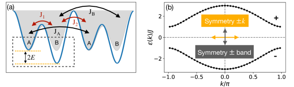
Figure 1: (a) A sketch of the Rice-Mele model in blue color, characterized by a staggered onsite potential, intracell hopping amplitude $J_{1}$, and intercell hopping amplitude $J_{2}$. $J_{A}$ and $J_{B}$ denote the next nearest neighbour hopping amplitudes. The potential can be realized by a superlattice, Eq. (21), in the experiments. The black dashed line indicates a unit cell. For $E=0$ one obtains the Su-Schrieffer-Heeger model as a filled gray color, which is characterized by a symmetric double-well system. (b) Single-particle energy spectrum for the SSH model with periodic boundary condition, i.e., Eq. (24) for $E=0$ and $J_{1}=2J_{2}=2J$. The symmetries related to $\pm k$ and between upper(+)/lower (-) bands are shown.

Our first example is the Rice-Mele model [40, 41], which describes a one-dimensional (1D) tight-binding chain with staggered hopping parameters and staggered on-site potentials [see sketch in Fig. 1(a)]. The Hamiltonian reads

$$H=\sum_{l}\left[E(n_{l,A}-n_{l,B})-\big{(}J_{1}a_{l,A}^{\dagger}a_{l,B}+J_{2}a_{l,B}^{\dagger}a_{l+1,A}+\mathrm{h.c.}\big{)}\right],$$ (20)

with $n_{l,\nu}=a_{l,\nu}^{\dagger}a_{l,\nu}$ being number operators for $\nu=A,B$. The chain consists of $N$ unit cells, each unit cell hosting two sites: one on sublattice $A$, one on sublattice $B$. Here, $J_{1}$ and $J_{2}$ denote the intracell and intercell nearest-neighbour tunnelling strength, and $E$ is the staggered onsite potential. This model can be realized with bichromatic ultracold atoms in optical lattices [42]. By using two counter propagating laser beams with period $d$ and $d/2$ respectively, one can obtain a superlattice with potential

$$V(x)=V_{1}\sin^{2}\left(\pi\frac{x}{d}\right)+V_{2}\sin^{2}\left(2\pi\frac{x}{d}+\theta\right),$$ (21)

where $\theta$ is the phase difference between these two different sublattices, and $V_{1}$ and $V_{2}$ are the lattice depths for the wider and narrower lattice, respectively.

For a translationally invariant chain with periodic boundary conditions (PBC), transforming the Hamiltonian to momentum space via $a_{k,A/B}^{\dagger}=\frac{1}{\sqrt{N}}\sum_{\ell}a_{\ell,A/B}^{\dagger}e^{ik\ell}$, where $k=q\frac{2\pi}{N}$ with $q=-\frac{N-1}{2},...,\frac{N-1}{2}$, yields

$$H=\sum_{k\in\mathcal{B}}(a_{k,A}^{\dagger},a_{k,B}^{\dagger})\mathcal{H}(k)\begin{pmatrix}a_{k,A}\\ a_{k,B}\end{pmatrix},$$ (22)

characterized by the single-particle Hamiltonian

$$\mathcal{H}(k)=\begin{pmatrix}E&-J_{1}-J_{2}e^{ik}\\ -J_{1}-J_{2}e^{-ik}&-E\end{pmatrix},$$ (23)

whose eigenenergies read

$$\varepsilon(k)=\pm\sqrt{E^{2}+(J_{1}+J_{2}\cos k)^{2}+(J_{2}\sin k)^{2}},$$ (24)

with the spectrum shown in Fig. 1(b) for $E=0$ and $J_{1}=2J_{2}$. The single-particle spectrum (24) has a symmetry with respect to $\pm k$ and a symmetry between upper and lower band. The former results from time-reversal invariance and the latter is a consequence of chiral symmetry, i.e., $\sigma_{z}{\cal H}(k)\sigma_{z}=-{\cal H}(k)$, with $\sigma_{z}$ being the Pauli matrix. Due to these symmetries, the many-body spectrum will be degenerate. For an effective cooling scheme, we need to lift the degeneracies in the half filling spectrum, which could be realized in different ways, such as by introducing a weak nearest-neighbour (NN) interaction under open boundary condition (OBC), or by introducing next-nearest-neighbour (NNN) tunneling under OBC, see more in A.

4.1.1 Feedback cooling of the SSH chain

For $E=0$ in the Hamiltonian (20), the Rice-Mele model reduces to the Su-Schrieffer-Heeger (SSH) model [39, 41]. The Su-Schrieffer-Heeger (SSH) model shows a topological phase transition at $J_{1}/J_{2}=1$, separating a topologically trivial phase for $J_{1}/J_{2}>1$ from a non-trivial one for $J_{1}/J_{2}<1$, which is characterized by a non-trivial winding of the Berry phase through the Brillouin zone. To study the effectiveness of the exact method, we first consider open SSH chains of moderate size ($N=1\sim 4$) at half filling that allow us to numerically solve the steady-state equation $\mathcal{L}\rho=0$ via time evolution of the system for sufficiently long time, with the superoperator $\mathcal{L}$ given in Eq. (8) and jump operator $C$ of Eq. (10). To lift degeneracies in the many-body spectrum (see Section 3.1), we further introduce a weak nearest-neighbour interaction

$$\hat{H}_{I}=U\sum_{\ell}(n_{\ell-1,B}n_{\ell,A}+n_{\ell,A}n_{\ell+1,B}).$$ (25)

We solve Eq. (8) numerically using the toolbox QuTiP [43] in Python to find the steady state. As expected by construction, the exact method always yields the desired state $\ket{g}$ with close-to-unity fidelity between the steady state and the ground state for all system sizes investigated numerically, both in the topological ($J_{1}/J_{2}<1$) and trivial ($J_{1}/J_{2}>1$) phase.

Considering now the approximate method, we construct analytically optimal states $\ket{b_{\ell,\pm}}$ of Eq. (16) which are used to define the jump operator $C_{\ell}$ of Eq. (15) localized in the $\ell$-th unit cell. In particular, we search for states such that $\ket{b_{\ell,-}}$ ($\ket{b_{\ell,+}}$) has minimal overlap with the upper (lower) band. The eigenvectors of the single-particle momentum-space Hamiltonian (23) for $E=0$ can be written as follows,

$$\ket{k_{\pm}}=\frac{1}{\sqrt{2}}\begin{pmatrix}\pm e^{i\phi_{k}}\\ 1\end{pmatrix},\qquad e^{i\phi_{k}}=\frac{-J_{1}-J_{2}e^{ik}}{|-J_{1}-J_{2}e^{ik}|}$$ (26)

The squared overlap of state $\ket{k_{\pm}}$ with $\ket{b_{\ell,-}}$ is thus

$$|\!\braket{k_{\pm}|b_{\ell,-}}\!|^{2}=\frac{1}{2N}\big{[}1\mp\sin(2\xi)\cos(\phi_{k})\big{]}.$$ (27)

Hence, the total overlap of the state $\ket{b_{\ell,-}}$ with the upper ($+$) and lower ($-$) band, shall be defined by the probability

$$\mathcal{P}_{\pm}(\xi)=\sum_{k\in\mathcal{B}}|\!\braket{k_{\pm}|b_{\ell,-}}\!|^{2} =\frac{1}{2}\mp\frac{\sin(2\xi)}{2N}\sum_{k\in\mathcal{B}}\cos(\phi_{k})$$ (28)

$$=\frac{1}{2}\mp\frac{\sin(2\xi)}{2N}s.$$ (29)

For convenience, in Eq. (29) we defined $s\equiv\sum_{k\in\mathcal{B}}\cos(\phi_{k})$, which is always negative for a large system with $J_{1}\neq 0$ and vanishes for $J_{1}=0$, since the $k$ values are equally spread over the first Brillouin zone.

Considering first $N=1$ for simplicity, we have $s=-1$. In this case, the minimal (maximal) overlap of $\ket{b_{\ell,-}}$ with the upper (lower) band is attained at $\xi=-\pi/4$, leading to states

$$\ket{b_{\ell,\pm}}=\frac{1}{\sqrt{2}}(\ket{\ell,A}\mp\ket{\ell,B}).$$ (30)

The orthogonality between $\ket{k_{+}}$ and $\ket{k_{-}}$ and between $\ket{b_{\ell,+}}$ and $\ket{b_{\ell,-}}$ then guarantees that $|\!\braket{k_{+}|b_{\ell,-}}\!|^{2}=|\!\braket{k_{-}|b_{\ell,+}}\!|^{2}$, such that $\ket{b_{\ell,+}}$ has minimal overlap with the lower band. We discuss below that this construction works well numerically also for larger $N$ for $J_{1}/J_{2}\gg 1$, while the regime $J_{1}/J_{2}\ll 1$ can be treated as well by a shift of the operators $\ket{b_{\ell,\pm}}$. With this choice for the states $\ket{b_{\ell,\pm}}$, the jump operator $C_{\ell}$ of Eq. (15) is determined as

$$C_{\ell}=\frac{\sqrt{\gamma}}{2}(n_{\ell,A}-n_{\ell,B})+\frac{\sqrt{\gamma}}{2}(a_{\ell,B}^{\dagger}a_{\ell,A}-a_{\ell,A}^{\dagger}a_{\ell,B}),$$ (31)

The corresponding measurement and feedback operators thus read

$$M_{\ell}=\frac{\sqrt{\gamma}}{2}(n_{\ell,A}-n_{\ell,B}),\qquad F_{\ell}=-i\frac{\sqrt{\gamma}}{2}(a_{\ell,A}^{\dagger}a_{\ell,B}-a_{\ell,B}^{\dagger}a_{\ell,A}).$$ (32)

Here, $M_{\ell}$ measures the population imbalance between the two sites $A$ and $B$ in the $\ell$-th unit cell, and $F_{\ell}$ denotes a tunneling between these two sites with a complex amplitude. The measurement of on-site population can be implemented via homodyne detection of the off-resonant scattering of structured probe light from the atoms [44, 45, 46]. The tunneling with a complex amplitude can be realized by accelerating the lattice [47, 34].

Figure 2(a) shows the minimal overlap $\sum_{k}|\!\braket{k_{+}|b_{\ell,-}}\!|^{2}$ between the state $|b_{\ell,-}\rangle$ given in Eq. (30) and the whole upper band. Figure 2(b) shows instead the fidelity given by the approximate cooling protocol as a function of $J_{1}/J_{2}$ for different system sizes ranging from 1 to 4 unit cells. As long as $J_{1}/J_{2}>1$ the fidelity is close to unity, while this is not the case for $J_{1}/J_{2}<1$ instead. This can be easily understood by considering that for $J_{1}>J_{2}$ the system dimerizes, with the dimers localized in each unit cell. Maximally localized Wannier functions of the form of $\ket{b_{\ell,\pm}}$ [Eq. (30)] can thus be constructed, which are mainly localized within the $\ell$th unit cell (B). For $J_{1}<J_{2}$, instead, the dimers straddle two neighbouring unit cells [41] and, in this case, the maximally localized Wannier functions also straddle two unit cells. Following this reasoning, successful cooling in the topological phase $J_{1}/J_{2}<1$ can also be achieved by choosing a collapse operator localized on neighbouring sites belonging to different unit cells. This can also be seen formally also from Eq. (28): in the limit $J_{2}=0$, it holds that $\cos(\phi_{k})=-1$ for any value of $k$, so the probability overlap ${\cal P}_{\pm}(\xi)=[1\pm\sin(2\xi)]/2$ can reach $0$ or $1$ for an appropriate choice of $\xi$, while in the limit $J_{1}=0$ it becomes $1/2$ for $N>1$ and is independent from $\xi$.

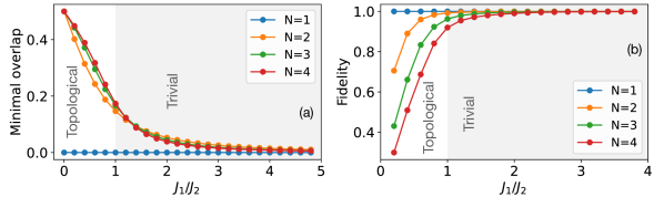
Figure 2: The approximate approach for the SSH model. The gray shaded background color indicates the trivial phase and the white background color indicates the topological phase. (a) The minimal overlap of Eq. (28) between the state $\ket{b_{\ell,-}}$ of lower band given by Eq. (30) and the upper band $\ket{k_{+}}$ for different small systems with $N$ unit cells as a function of $J_{1}/J_{2}$. (b) Fidelity defined in Eq. (19) as a function of $J_{1}/J_{2}$ with open boundary conditions for different small systems with $N$ unit cells. The steady state $\rho_{\rm ss}$ is obtained via time evolution of the system according to Eq. (8) with the jump operator constrained to two sites within one unit cell given by Eq. (31). The measurement strength is set to $\gamma=0.0001J$ with $J$ the energy unit.

4.1.2 Rice-Mele pumping cycle

We now construct the approximate jump operator $C_{\ell}$ for the Rice-Mele model of Eq. (20) with a non-zero staggered on-site potential $E\neq 0$. A state in the upper band can be written in the form

$$\ket{k_{+}}=\cos\frac{\chi_{k}}{2}\ket{k,A}+e^{-i\phi_{k}}\sin\frac{\chi_{k}}{2}\ket{k,B},$$ (33)

where $\chi_{k}=2\arctan\big{[}(\sqrt{E^{2}+J^{2}}-E)/J\big{]}$ with $-J_{1}-J_{2}e^{ik}=Je^{i\phi_{k}}$. The squared overlap $\mathcal{P}_{+}(\xi)$ of $\ket{b_{\ell,-}}$ defined in Eq. (16) with the whole upper band is then

$$\mathcal{P}_{+}(\xi)=\frac{1}{2}\left\{1-\frac{1}{N}\cos(2\xi)\sum_{k\in\mathcal{B}}\cos\chi_{k}-\frac{1}{N}\sin(2\xi)\sum_{k\in\mathcal{B}}\sin\chi_{k}\cos(\phi_{k})\right\}.$$ (34)

If $\sum_{k\in\mathcal{B}}\cos\chi_{k}\neq 0$ and $2\xi\neq(n+1/2)\pi$ with integer $n$, the extremal point satisfies

$$\tan{2\xi}=\frac{\sum_{k\in\mathcal{B}}\sin\chi_{k}\cos(\phi_{k})}{\sum_{k\in\mathcal{B}}\cos\chi_{k}}.$$ (35)

With the approximate cooling operator determined by $\xi$, we study the cooling during a Rice-Mele pumping cycle. In this process, the parameters $E$, $J_{1}$ and $J_{2}$ in the Hamiltonian (20) are modulated periodically in time in a slow, adiabatic fashion. Through an appropriate parameter variation, the modulation pumps an integer number of particles along the chain which is determined by the Chern number of the valence band [48]. This so-called topological charge pump that can be thought of as a 1D analog of the quantum Hall effect, where one spatial dimension is substituted by the temporal one [49].

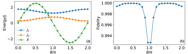
Figure 3: The approximate method for a Rice-Mele pumping cycle. (a) Hopping amplitudes $J_{1}$, $J_{2}$ and onsite potential $E$ as a function of $\theta$ given by Eq. (36). (b) Fidelity defined in Eq. (19) during the pumping cycle as a function of $\theta$ for a small system with 3 unit cells under open boundary condition. The steady state $\rho_{\rm ss}$ is given by Eq. (8) and the jump operator constrained to two sites within one unit cell is given by Eq. (31). The measurement strength is set to $\gamma=0.0001J$ with $J$ the energy unit. The steady state is obtained via time evolution of the system according to Eq. (8).

We consider the following modulation of the on-site potential and hopping parameters [42, 50],

$$E(\theta)=\frac{5J}{2}\sin\theta\ ,\qquad J_{1}(\theta)=\frac{J}{2}\left[3+\frac{1}{2}\cos\theta\right]\ ,\qquad J_{2}(\theta)=\frac{J}{2}\left(1-\frac{1}{2}\cos\theta\right)\$$ (36)

as depicted in Fig. 3(a), with $J$ the energy unit. In an experiment, the modulation is achieved by varying the phase difference $\theta$ between the two sublattices, see Eq. (21). The cooling fidelity is reported in Fig. 3(b) as a function of $\theta$. In a large parameter regime, the deviation from unity is less than $10^{-3}$ and it remains always well below one percent, indicating that the approximate cooling protocol is reliable during the whole pumping cycle. The fidelity is slightly lower (although by a few parts in a thousand only) for values around $\theta\simeq\pi$. This effect can be explained by noting that at such values the on-site potential is close to zero. Non-zero values of $E$ indeed contribute in effectively reducing the hopping amplitude by bringing nearby sites off-resonant, thus favouring localized states that are well described by the single-cell ansatz (17) used for $\ket{b_{\ell,\pm}}$.

4.2 Two-dimensional topological insulator: The Haldane model

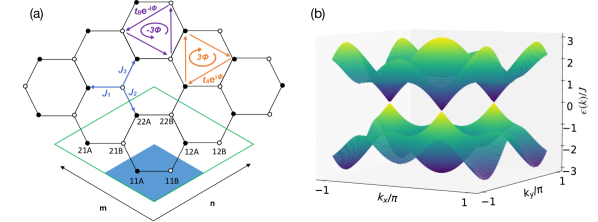
Figure 4: (a) Haldane model with hopping vectors in real space. The region in blue shading shows one unit cell with two sites $A$ and $B$. $J_{1}$, $J_{2}$ and $J_{3}$ are the nearest neighbour hopping amplitudes. The next nearest neighbour (NNN) hopping in a clockwise closed path with magnetic flux $3\phi$ enclosed is shown in orange color and the corresponding NNN hopping acquires a complex phase $e^{i\phi}$, and vice versa, the anticlockwise NNN hopping acquires a complex phase $e^{-i\phi}$. In order to enumerate the unit cells, we consider two directions with labels $m$ and $n$, which take integer values. Each lattice site is described by three parameters: $mn\sigma$, with $mn$ the index of unit cell and $\sigma=A,B$. (b) Single particle spectrum under periodic boundary condition for the Haldane model with $J_{\lambda}=J$, $t_{A}=t_{B}=0.1J$, $\phi=\pi/2$, $\Delta=0.52J$.

After having demonstrated the effectiveness of the cooling protocols in one-dimensional topological insulators, we now address the case of a two-dimensional system: the Haldane model of a Chern insulator [2]. This model substantially differs from previous examples, both because of its dimensionality and of its topological characterization. The Haldane model is defined on a honeycomb lattice with two sites ($A$ and $B$) per unit cell, as shown in Fig. 4(a). In order to enumerate the unit cells, we consider two directions with labels $m$ and $n$, which take integer values. Each lattice site is described by three parameters: $mn\sigma$, with $mn$ the index of unit cell and $\sigma=A,B$. The Hamiltonian is given by

$$H=-\sum_{\langle i,j\rangle_{\lambda=1,2,3}}J_{\lambda}\left(a_{i}^{\dagger}b_{j}+h.c.\right)-\sum_{\begin{subarray}{c}\langle\!\langle i,j\rangle\!\rangle_{\sigma=A,B}\\ c=a,b\end{subarray}}t_{\sigma}\left(c_{i}^{\dagger}c_{j}e^{i\nu_{ij}\phi}+h.c.\right)+\Delta\sum_{i}\left(a_{i}^{\dagger}a_{i}-b_{i}^{\dagger}b_{i}\right)\ .$$ (37)

The summation over $\langle i,j\rangle_{\lambda}$ runs over (ordered) pairs of nearest neighbours (NN) with $\lambda=1,2,3$, as shown in Fig. 4(a), while the summation over $\langle\!\langle i,j\rangle\!\rangle_{A/B}$ runs over next-nearest neighbours (NNN) between $AA$ or $BB$ sites. The complex phases $e^{i\nu_{ij}\phi}$ can be thought of as resulting from a magnetic field penetrating the lattice with zero net flux in each hexagon. The value of $\nu_{ij}$ is determined by the hopping directions with $\nu_{ij}=1$ for clockwise hopping and $\nu_{ij}=-1$ for counterclockwise hopping. The Haldane Hamiltonian thus features real-valued NN hopping parameters ($-J_{\lambda}$) and complex NNN hopping parameters ($-t_{\sigma}e^{i\nu_{ij}\phi}$). We consider first the original Haldane model with $J_{\lambda}=J$ and $t_{\sigma}=t$, if not otherwise mentioned. The complex NNN coupling matrix elements break time-reversal symmetry and open gaps at both of the Dirac-type band-touching points, so that the resulting individual bands require topologically non-trivial properties characterized by Chern numbers $\pm 1$. In turn, the energy offset $\Delta$ breaks inversion symmetry. This term alone would open a topologically trivial band gap. If both terms are present, we find a competition between the two. By varying $\Delta$, the system enters a topological phase when $|\Delta|<|3\sqrt{3}t\sin\phi|$, which is characterized by the appearance of the chiral edge states [51].

4.2.1 Exact vs approximate method in small systems

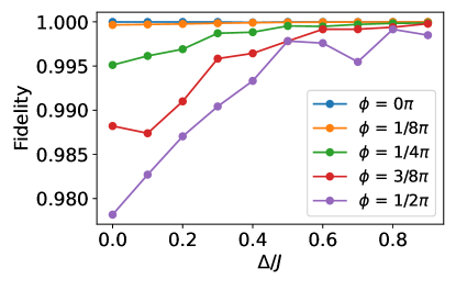
Figure 5: Fidelity between the steady state given by Eq. (8) with jump operator $C$ of Eq. (10) (for the exact approach) and the ground state of the Haldane model (37) for a small system with 4 unitcells as a function of the onsite potential $\Delta$ for different complex hopping phase $\phi$, which is given in units of $\pi$. The steady state is obtained via time evolution of the system according to Eq. (8). We use OBC with small interaction (25) of strength $0.001J$ to break the degeneracy.

To investigate feedback cooling in the Haldane model, we first focus on a system with $N=4$ unit cells as depicted with green line in Fig. 4(a). The steady state is obtained via time evolution of the system according to Eq. (8) as done for the Rice-Mele model. Unwanted degeneracies arising from the symmetric single-particle spectrum shown in Fig. 4(b) are lifted by using open boundary conditions and adding a small nearest-neighbour interaction, see Eq. (25). The fidelity given by the exact method is shown in Fig. 5 for different values of the NNN tunneling phase $\phi$. As for the 1D case, the fidelity is very close to one for all parameter values, confirming the efficiency of the exact method.

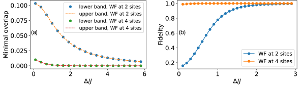
Figure 6: Approximate approach for a small system of the Haldane model with 4 unitcells as depicted with green line in Fig. 4(a). We consider the cases where the wavefunctions (WF) $\ket{b_{\pm}^{\mathcal{S}_{n}}}$ localized at two sites with indices $11A$, $11B$ in the first unit cell, and on four sites with indices $11A$, $11B$, $21B$, $12A$ indicated in Fig. 4(a). We set $\phi=\pi/2$ and $t=0.1J$ with the energy unit $J$, which is the NN hopping amplitude. The paramerizations of $\ket{b_{\pm}^{\mathcal{S}_{n}}}$ are given by Eq. (17) for $n=2$ and by Eq. (4.2.1) for $n=4$. The parameters can be determined by minimizing the overlap of $\ket{b_{-}^{\mathcal{S}_{n}}}$ ($\ket{b_{+}^{\mathcal{S}_{n}}}$) with upper (lower) band, with the minimal overlaps shown in (a). (b) Fidelity between the steady state given by Eq. (8) and the ground state of the Haldane model for a small system with 4 unitcells as a function of the onsite potential $\Delta$ for $t=0.1J$ with $J$ the NN hopping amplitude. The steady state is obtained via time evolution of the system according to Eq. (8) with the jump operator $C_{\mathcal{S}_{n}}=(b_{-}^{\mathcal{S}_{n}})^{\dagger}b_{+}^{\mathcal{S}_{n}}$. The measurement strength is set to $\gamma=0.0001J$.

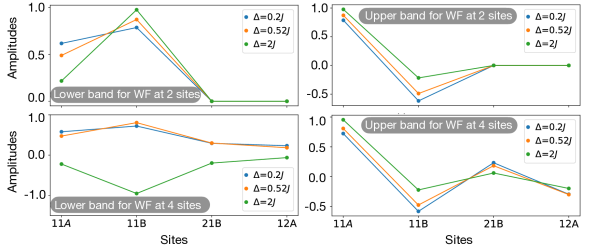
Figure 7: Amplitudes of the optimal wavefunctions $\ket{b_{\ell=1,\pm}}$ at two sites in the first unit cell with the ansatz given by Eq. (17) and $\ket{b_{\pm}^{\mathcal{S}_{4}}}$ at four sites with the ansatz given by Eq. (4.2.1). The different colors stand for different on-site potentials $\Delta$. We consider a small system of the Haldane model with 4 unitcells as depicted with green line in Fig. 4(a). We set $\phi=\pi/2$ and $t=0.1J$ with $J$ the NN hopping amplitude. To get the optimal parameters we try to minimize the overlap of $\ket{b_{-}^{\mathcal{S}_{n}}}$ ($\ket{b_{+}^{\mathcal{S}_{n}}}$) with upper (lower) band. We choose the two sites with indices $11A$, $11B$ in the first unit cell, and the four sites with indices $11A$, $11B$, $21B$, $12A$, as shown in Fig. 4(a).

We then test the approximate method by constructing constrained jump operators localized at two sites with indices $11A$, $11B$ in the first unit cell, and on four sites with indices $11A$, $11B$, $21B$, $12A$ indicated in Fig. 4(a). We can parameterize the wavefunctions localized at four sites with three parameters $\xi_{1}$, $\xi_{2}$ and $\xi_{3}$ in the following way,

$$\ket{b_{\pm}^{\mathcal{S}_{4}}}= \sin(\xi_{1})\sin(\xi_{2})\sin(\xi_{3})\ket{11A}+\sin(\xi_{1})\sin(\xi_{2})\cos(\xi_{3})\ket{11B}$$

$$+\sin(\xi_{1})\cos(\xi_{2})\ket{21B}+\cos(\xi_{1})\ket{12A}.$$ (38)

Given the parametrization (4.2.1) the optimal parameters $\xi_{1}$, $\xi_{2}$ and $\xi_{3}$ can be determined by following the similar strategy as the two sites case, where we try to minimize the overlap of $\ket{b_{-}^{\mathcal{S}_{4}}}$ ($\ket{b_{+}^{\mathcal{S}_{4}}}$) with upper (lower) band, with the minimal overlaps shown in Fig. 6(a). For smaller on-site potential $\Delta$ (corresponding to the topological phase) the minimal overlaps are smaller for $\ket{b_{\pm}^{\mathcal{S}_{n}}}$ localized at four sites than at two sites. The amplitudes of the optimal wavefunction $\ket{b_{\pm}^{\mathcal{S}_{n}}}$ at different lattice sites are shown in Fig. 7. The resulting fidelity is shown in Fig. 6(b). For the two-site jump operator $C_{\mathcal{S}_{2}}$ the cooling is not efficient for small on-site potentials $\Delta/J\ll 1$, but the fidelity grows monotonically by increasing $\Delta$, eventually reaching $\mathcal{F}=1$ for $\Delta/J\sim 3$. The situation strikingly improves when considering $C_{\mathcal{S}_{4}}$, localized on four sites. In this case the fidelity barely deviates from one at vanishing $\Delta$, and remains otherwise very close to one for all values of $\Delta$. For small on-site potentials, the 2D system is in a topological phase and it is not possible to construct maximally localized Wannier functions [51], which leads to poor cooling performance of the two-sited algorithm. This differs significantly from the 1D SSH model 4.1.1, where cooling in the topological phase still works by simply shifting the operators $\ket{b_{\ell,\pm}}$, as the maximally localized Wannier functions are shifted in this case.

4.2.2 Cooling large systems: mean-field approach

Having benchmarked the performance of both the exact and the approximate methods in small systems by exact numerical determination of the steady state, we now investigate cooling in the (non-interacting) Haldane model for larger systems by adopting a mean-field approach. In particular, following Refs. [52, 53] we derive kinetic equations of motion for the mean occupations of the single-particle eigenstates (C). The resulting non-linear equations of motions read

$$\frac{d}{dt}\bar{n}_{k}(t)=\sum_{q}\Big{(}R_{kq}\bar{n}_{q}[1-\bar{n}_{k}(t)]-R_{qk}\bar{n}_{k}(t)[1-\bar{n}_{q}(t)]\Big{)},$$ (39)

where $\bar{n}_{k}(t)=\mathrm{tr}[n_{k}\rho(t)]$ is the mean occupation number of the $k$-th single-particle eigenstate (ordered by increasing energy). These equations are obtained by neglecting non-trivial correlations, $\mathrm{tr}[n_{k}n_{q}\rho(t)]\approx\bar{n}_{k}(t)\bar{n}_{q}(t)$, which is justified in the limit of large systems. The transition rates $R_{kq}$ are obtained from the feedback master equation (7) after an additional rotating-wave-approximation (RWA), which is valid if the single-particle energy gaps and their differences are much larger than the measurement strength $\gamma$. The rates are derived from the feedback jump operator $C$ according to $R_{kq}=|C_{kq}|^{2}$.

In the case of the exact method, we see from Eq. (12) that the rates $R_{kq}$ are such that $R_{kq}=1$ (in the dimensionless units used), if the eigenstates labeled by $k$ and $q$ belong to the lower and upper band, respectively, while $R_{kq}=0$ otherwise. The mean-field equation (39) for the occupation of a state $k$ in the lower band then reduces to

$$\frac{d}{dt}\bar{n}_{k}(t)=[1-\bar{n}_{k}(t)]\sum_{q\in B_{+}}\bar{n}_{q}(t),$$ (40)

where $B_{+}$ denotes the upper band. The steady state, $d\bar{n}_{k}(t)/dt=0$, is then easily found to be $\bar{n}_{k}(t)=1$, confirming that an exact preparation of the many-body ground state is indeed attained, featuring all states in the lower band occupied.

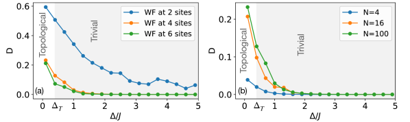
Figure 8: Efficiency of the approximate construction for the Haldane model. We plot the deviation given by (41) between the steady state of the mean-field equations (39) and the ground state as a function of on-site potential $\Delta$ for $\phi=\pi/2$. We consider slightly different NNN hoppings with $t_{A}=0.1J$, $t_{B}=0.05J$, where $t_{A}$ denotes the NNN hopping amplitude without phase factor for $AA$ sites and $t_{B}$ denotes the NNN hopping amplitude without phase factor for $BB$ sites. $\Delta_{T}$ denotes the topological phase transition. (a) We consider a large system with 100 unit cells arranged in $10\times 10$ , as shown in Fig. 4(a). The wavefunctions are constrained at two, four or six sites . The choice of $\mathcal{S}_{2}$ and $\mathcal{S}_{4}$ is same with Fig. 6. $\mathcal{S}_{6}$ is given by $11A$, $11B$, $21B$, $12A$, $22A$ and $22B$ as indicated in Fig. 4(a). (b) Deviation for different large systems with $N$ unit cells arranged in a manner such that $m$ and $n$ run from 1 to $\sqrt{N}$, as shown in Fig. 4(a). The wavefunctions are constrained at four sites with the choice of $\mathcal{S}_{4}$ same with (a).

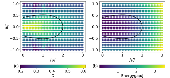
Figure 9: Energy gaps (a) under open boundary conditions and Deviation (b) between final state of the mean-field equations (39) and ground state of the Haldane model for a large system with 16 unitcells arranged in the same way as Fig. 8. The approximate approach with wavefunctions localized at 2 sites is applied here. The parameters are set as $J_{2}=J_{3}=J$ and $t=0.1J$. The black curves describe the topological transition, which is given by Eq. (42). The horizontal axis is $J_{1}$ and vertical axis is the on-site potential $\Delta$. The deviation $D$ given by (41) and the energy gap, which are functions of $J_{1}$ and $\Delta$, are represented with a color map.

We then investigate the performance of the approximate method by constraining the jump operator to different sets of sites $\mathcal{S}_{n}$ and solving the mean field equations (39) numerically in a system of $N=100$ unit cells arranged in a manner such that $m$ and $n$ run from 1 to 10, as shown in Fig. 4(a). To ensure that the spectrum does not feature two identical level spacings (see C), such that the RWA can be assumed to be valid for a suitably small $\gamma$, we consider slightly different strength of the NNN hopping between two $A$ sites, denoted with $t_{A}$, as compared to two $B$ sites, denoted with $t_{B}$ (see Fig. 4(a)). The construction of the constrained jump operators is performed via numerical optimization as explained in Section 3.3. We quantify the deviation $D(\bar{\bm{n}})$ from the ground state by comparing the mean occupation numbers in the steady state, $\bar{\bm{n}}=\{\bar{n}_{k}\}_{k=1,\dots,2N}$ with those in the ground state, $\bar{\bm{n}}^{(g)}=\{\bar{n}_{k}^{(g)}\}_{k=1,\dots,2N}$, computing

$$D(\bar{\bm{n}})=\sqrt{\frac{1}{2N}\sum_{k=1}^{2N}(\bar{n}_{k}-\bar{n}_{k}^{(g)})^{2}}.$$ (41)

The sets $\mathcal{S}_{n}$ considered are localized on $n=2$, 4 and 6 sites. The choice of $\mathcal{S}_{2}$ and $\mathcal{S}_{4}$ is the same with Fig. 6. $\mathcal{S}_{6}$ is given by $11A$, $11B$, $21B$, $12A$, $22A$ and $22B$ as indicated in Fig. 4(a). The deviation $D$ obtained as a function of $\Delta$ is depicted in Fig. 8. We observe that the deviation is fairly large for $\mathcal{S}_{2}$ (blue curve), but it gets much closer to zero as the number of sites is increased, for $\mathcal{S}_{4}$ (orange curve) and $\mathcal{S}_{6}$ (green curve). In the latter cases, the deviation tends to zero for $\Delta/J>1$, but deviates from zero for $\Delta/J<1$.

The above effect can be understood in the light of the topological phase transition, thus interestingly linking the efficiency of the engineered cooling mechanism with the system’s topological properties. Indeed, around $0<\Delta_{T}<1$, the system crosses the phase transition and enters the topological phase, where exponentially localized Wannier functions do not exist, such that the constrained ansatz states $\ket{b_{\pm}^{\mathcal{S}_{n}}}$ cannot reproduce the eigenstates to a satisfactory degree. To bring further evidence that this effect is indeed related to the topological phase transition, we show in Fig. 8(b) the deviation for different system sizes, again as a function of $\Delta$. The steepness of the curve at low $\Delta$ increases for increasing size, as expected, since it is more difficult to find Wannier functions localized at four sites in topological phase. As an additional signature, we study how the cooling improves by entering a trivial dimerized phase, in which the tunneling strength $J_{1}$ along the direction $e_{1}$ is much larger than in other directions [see Fig. 4(a)]. For the case of a dimerization with changing $J_{1}$ and constant $J_{2}=J_{3}=J$ the topological phase transition is given by

$$\Delta\pm t\left(\frac{J_{1}}{J}+2\right)\sqrt{4-\frac{J_{1}^{2}}{J^{2}}}=0.$$ (42)

The deviation for this case is reported in Fig. 9(a), and indeed becomes smaller for increasing $J_{1}$. This observation together with the results in Fig. 8 indicate that the deviation is related with the energy gap, so we plot the energy gaps of the Haldane model in Fig. 9 for the approximate approach with jump operators localized at two sites under open boundary condition. We observe that $D$ is smaller (larger) for a larger (smaller) energy gap, which indicates that the cooling performance is much better for a larger energy gap.

5 Conclusions

In summary, we have proposed a scheme to prepare topological insulator states for noninteracting fermionic atoms in an optical lattice through Markovian feedback control. Specifically, we considered topologically non-trivial two-band models at half-filling, and exploited continuous weak measurement and Markovian feedback to engineer a dissipative process which cools the system towards the ground state. This is achieved, in turn, by constructing a dissipative process that pumps particles from the upper band to the lower band, until the latter is filled. We further propose approximate variant schemes that can perform the same task with lower efficiency, when additional experimental constraints on the measurement and feedback apparatus are introduced. We have benchmarked these two approaches in several 1D and 2D lattice models, namely for the Su-Schrieffer-Heeger model, the Rice-Mele model and the Haldane model. For moderate system sizes, we probed the steady state of the system via time evolution of the system according to the feedback-modified master equation. For large systems, we resorted to kinetic theory and compare the mean occupations in the single-particle eigenstates. The proposed exact cooling scheme is successful in all parameter regimes and for all models studied. The approximate methods, which involve a restriction of the measurement and feedback operations to small subsystems, give good performance for small systems or when the system eigenstates tend to be localized on few sites. While this makes this approach less effective in the topological phase of the 2D Haldane model for large systems, it still gives a satisfactory preparation of TI states in the 1D models studied.

Appendix A Different methods to lift degeneracies of the many-body spectrum

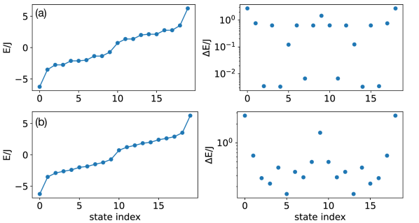
Figure 10: Half-filling spectrum for a system of 3 unit cells in SSH model with $J_{1}=2J$ and $J_{2}=J$. The eigenenergies are sorted in an ascending way and enumerated along the x-axis. Figures on the left side are plots of the energy spectrum in linear scale. Figures on the right side are in semilog scale and describe the energy difference between neighboring points of the left plots. (a) Plots for the case of OBC with small interaction of strength 0.01J. (b) Plots for the case of OBC with NNN hopping strength 0.1J.

The degeneracies in the many-body spectrum arise from the symmetric single-particle spectrum with respect to $\pm k$ and between the two bands, as shown in Fig. 1(b). We study different ways to lift the degeneracies.
(1) We introduce a small interaction between nearest neighbors with interaction Hamiltonian in Eq. (25), with $U$ denoting the interaction strength, and use open boundary conditions (OBC). For OBC $l$ runs from 1 to $N-1$ in Eq. (20). We plot the half-filling spectrum and the energy difference between neighbouring states in Fig. 10(a), where all the energy differences $\Delta E$ are non-zero, which means that the degeneracy is lifted by adding small nearest-neighbour interactions.
(2) We can introduce more tunneling coefficients, such as next nearest neighbor tunneling coefficients (NNN hopping). Similar as in (1), the half-filling spectrum and the energy differences are plotted in Fig. 10(b).

Appendix B Maximally localized Wannier function in SSH model

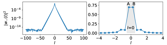
Figure 11: MLWF in tight binding model for SSH model with 201 unit cells with $J_{1}=2J_{2}$, for the lower ($-$) band. The index $l$ lists all unit cells from -100 to 100. The gray region shows the 0th unit cell with $A$ and $B$ sites. In this case the Wannier function is exponentially localized. Plots on the left side are in semilog scale. Plots on the right side are in linear scale and zoom on the peak of the Wannier functions.

We recall that Wannier functions are used to construct the collapse operators in Eq. (12). The approximate approach, where the collapse operator is chosen to be localized at a few sites, is based on the fact that by choosing appropriate gauge factors it is possible to find well localized Wannier states in Eq. (12). Here, as an example, we try to construct maximally localized Wannier function $\ket{W_{-}(l)}$ in the tight binding SSH model with $J_{1}=2J_{2}$, for the lower ($-$) band, where $l$ lists all unit cells. In order to find the appropriate gauge factor $e^{i\varphi_{k_{-}}}$, we perform either a single-band transformation following Ref. [54] or use the Kohn gauge [55]. In the Kohn gauge, the gauge factor can be chosed as

$$\varphi_{k_{-}}=-{\rm arg}(\ket{k_{-}}_{1}+\ket{k_{-}}_{2}),$$ (43)

where $\ket{k_{-}}_{1}$ and $\ket{k_{-}}_{2}$ are the two components of the lower band eigenvector $\ket{k_{-}}$ in Eq. (26). The computed Wannier function is shown in Fig. 11, where we notice an exponential localization of the Wannier function in space. We can calculate the weight of the two sites $0A$ and $0B$ in the 0th unit cell, which is $|w_{-}(0A)|^{2}+|w_{-}(0B)|^{2}=0.97$, where the Wannier function is normalized. This result implies that the approximate approach for SSH model should work very well for $J_{1}=2J_{2}$, which is consistent with the results in Fig. 2.

Appendix C Derivation of the mean-field equations

Since it is very demanding to calculate the steady state $\rho_{ss}$ numerically for large systems, we can adopt a mean-field description in which we rather study the time evolution of the mean occupation of single-particle eigenstates, following Refs. [52, 53]. To work out this mean-field description, we first need to recast the master Eq. (7) (with $H_{\rm fb}=0$) in a form which describes quantum jumps between single-particle eigenstates. This can be achieved, while maintaining Lindblad form, as follows. We first represent the collapse operator $C$ in the system’s eigenbasis, $C=\sum_{k,q}C_{kq}a_{k}^{\dagger}a_{q}=\sum_{k,q}C_{kq}L_{kq}$, where $L_{kq}=a_{k}^{\dagger}a_{q}$ describes a quantum jump from single-particle eigenstate $\ket{q}$ to $\ket{k}$. In interaction picture, the master equation then reads as

$$\frac{d\rho}{dt}=\sum_{k,q,k^{\prime},q^{\prime}}C_{kq}C_{k^{\prime}q^{\prime}}^{*}e^{i(\omega_{kq}-\omega_{k^{\prime}q^{\prime}})t}\Big{[}L_{kq}\rho L_{k^{\prime}q^{\prime}}^{\dagger}-\frac{1}{2}L_{k^{\prime}q^{\prime}}^{\dagger}L_{kq}\rho-\frac{1}{2}\rho L_{k^{\prime}q^{\prime}}^{\dagger}L_{kq}\Big{]},$$ (44)

where $\omega_{kq}=\epsilon_{k}-\epsilon_{q}$ is the energy difference between the single-particle levels $\epsilon_{k}$ and $\epsilon_{q}$. To achieve an equation in Lindblad form, we next adopt the rotating-wave (secular) approximation, which amounts to neglect oscillating terms in Eq. (44). This is justified only in the regime where the difference in level spacings $\omega_{kq}-\omega_{k^{\prime}q^{\prime}}$ is much larger than the measurement strength $\gamma$, $|\omega_{kq}-\omega_{k^{{}^{\prime}}q^{{}^{\prime}}}|\gg\gamma$. To ensure that this condition can be met, in our numerical studies we use the methods described in A to prevent the emergence of identical level spacings in the single-particle spectrum. In rotating-wave approximation, Eq. (44) then becomes

$$\frac{d\rho}{dt}=\sum_{k,q}R_{kq}\Big{[}L_{kq}\rho L_{kq}^{\dagger}-\frac{1}{2}L_{kq}^{\dagger}L_{kq}\rho-\frac{1}{2}\rho L_{kq}^{\dagger}L_{kq}\Big{]},$$ (45)

where we introduced the effective quantum jump rates $R_{kq}=|C_{kq}|^{2}$. From Eq. (45), one can derive an Eq. ruling the evolution of the single-particle occupations $\bar{n}_{k}=\mathrm{tr}(\rho n_{k})$. The latter will also depend on two-particle correlations, $\mathrm{tr}(\rho n_{k}n_{q})$, initiating a hierarchy of Eqs. for the $n$-particle correlation functions [53]. The hierarchy can be truncated in a mean-field-like approximation by assuming the factorization of two-particle correlations, $\mathrm{tr}(\rho n_{k}n_{q})\approx\bar{n}_{k}\bar{n}_{q}$ [53]. This procedure yields non-linear mean-field equations for the single-particle occupations, reading as

$$\frac{d}{dt}\bar{n}_{k}(t)\approx\sum_{q}\left\{R_{kq}\bar{n}_{q}(t)[1-\bar{n}_{k}(t)]-R_{qk}\bar{n}_{k}(t)[1-\bar{n}_{q}(t)]\right\}.$$ (46)

In the main text, we studied the steady-state occupations given by these mean-field equations, satisfying $\frac{d}{dt}\bar{n}_{k}(t)=0$, which have been found numerically both via long-time propagation and through a nonlinear-equation solver.

References

- [1] M.. Hasan and C.. Kane “Colloquium: Topological insulators” In Rev. Mod. Phys. 82 American Physical Society, 2010, pp. 3045 DOI: 10.1103/RevModPhys.82.3045
- [2] F… Haldane “Model for a Quantum Hall Effect without Landau Levels: Condensed-Matter Realization of the ”Parity Anomaly”” In Phys. Rev. Lett. 61 American Physical Society, 1988, pp. 2015 DOI: 10.1103/PhysRevLett.61.2015
- [3] D.. Thouless, M. Kohmoto, M.. Nightingale and M. Nijs “Quantized Hall Conductance in a Two-Dimensional Periodic Potential” In Phys. Rev. Lett. 49 American Physical Society, 1982, pp. 405 DOI: 10.1103/PhysRevLett.49.405
- [4] B. Bernevig “Topological Insulators and Topological Superconductors” Princeton University Press, 2013
- [5] K.. Klitzing, G. Dorda and M. Pepper “New Method for High-Accuracy Determination of the Fine-Structure Constant Based on Quantized Hall Resistance” In Phys. Rev. Lett. 45 American Physical Society, 1980, pp. 494 DOI: 10.1103/PhysRevLett.45.494
- [6] Richard E. Prange and Steven M. Girvin “The Quantum Hall Effect” Springer-Verlag, 1990 DOI: 10.1007/978-1-4612-3350-3
- [7] Gregor Jotzu et al. “Experimental realization of the topological Haldane model with ultracold fermions” In Nature 515, 2014, pp. 237–240 DOI: 10.1038/nature13915
- [8] M. Aidelsburger et al. “Measuring the Chern number of Hofstadter bands with ultracold bosonic atoms” In Nat. Phys. 11, 2015, pp. 162–166 DOI: 10.1038/nphys3171
- [9] M. Tai et al. “Microscopy of the interacting Harper–Hofstadter model in the two-body limit” In Nature 546, 2017, pp. 519–523 DOI: 10.1038/nature22811
- [10] K. Wintersperger et al. “Realization of an anomalous Floquet topological system with ultracold atoms” In Nat. Phys. 16, 2020, pp. 1058–1063 DOI: 10.1038/s41567-020-0949-y
- [11] André Eckardt “Colloquium: Atomic quantum gases in periodically driven optical lattices” In Rev. Mod. Phys. 89 American Physical Society, 2017, pp. 011004 DOI: 10.1103/RevModPhys.89.011004
- [12] S. Diehl et al. “Quantum states and phases in driven open quantum systems with cold atoms” In Nat. Phys. 4, 2008, pp. 878–883 DOI: 10.1038/nphys1073
- [13] B. Kraus et al. “Preparation of entangled states by quantum Markov processes” In Phys. Rev. A 78 American Physical Society, 2008, pp. 042307 DOI: 10.1103/PhysRevA.78.042307
- [14] Frank Verstraete, Michael M. Wolf and J. Ignacio Cirac “Quantum computation and quantum-state engineering driven by dissipation” In Nat. Phys. 5, 2009, pp. 633–636 DOI: 10.1038/nphys1342
- [15] Alexander Schnell, Ling-Na Wu, Artur Widera and André Eckardt “Floquet-heating-induced Bose condensation in a scarlike mode of an open driven optical-lattice system” In Phys. Rev. A 107 American Physical Society, 2023, pp. L021301 DOI: 10.1103/PhysRevA.107.L021301
- [16] Francesco Petiziol and André Eckardt “Controlling nonequilibrium Bose-Einstein condensation with engineered environments” In Phys. Rev. A 110 American Physical Society, 2024, pp. L021701 DOI: 10.1103/PhysRevA.110.L021701
- [17] Sebastian Diehl, Enrique Rico, Mikhail A. Baranov and Peter Zoller “Topology by dissipation in atomic quantum wires” In Nat. Phys. 7, 2011, pp. 971–977 DOI: 10.1038/nphys2106
- [18] N. Goldman, J.. Budich and P. Zoller “Topological quantum matter with ultracold gases in optical lattices” In Nat. Phys. 12, 2016, pp. 639–645 DOI: 10.1038/nphys3803
- [19] Moshe Goldstein “Dissipation-induced topological insulators: A no-go theorem and a recipe” In SciPost Phys. 7 SciPost, 2019, pp. 67 DOI: 10.21468/SciPostPhys.7.5.067
- [20] Tao Qin et al. “Charge density wave and charge pump of interacting fermions in circularly shaken hexagonal optical lattices” In Phys. Rev. A 98 American Physical Society, 2018, pp. 033601 DOI: 10.1103/PhysRevA.98.033601
- [21] Souvik Bandyopadhyay and Amit Dutta “Dissipative preparation of many-body Floquet Chern insulators” In Phys. Rev. B 102 American Physical Society, 2020, pp. 184302 DOI: 10.1103/PhysRevB.102.184302
- [22] Karthik I. Seetharam et al. “Controlled Population of Floquet-Bloch States via Coupling to Bose and Fermi Baths” In Phys. Rev. X 5 American Physical Society, 2015, pp. 041050 DOI: 10.1103/PhysRevX.5.041050
- [23] Eliot Kapit, Mohammad Hafezi and Steven H. Simon “Induced Self-Stabilization in Fractional Quantum Hall States of Light” In Phys. Rev. X 4 American Physical Society, 2014, pp. 031039 DOI: 10.1103/PhysRevX.4.031039
- [24] Zhao Liu, Emil J. Bergholtz and Jan Carl Budich “Dissipative preparation of fractional Chern insulators” In Phys. Rev. Res. 3, 2021, pp. 043119 DOI: 10.1103/physrevresearch.3.043119
- [25] Francesco Petiziol and André Eckardt “Cavity-Based Reservoir Engineering for Floquet-Engineered Superconducting Circuits” In Phys. Rev. Lett. 129 American Physical Society, 2022, pp. 233601 DOI: 10.1103/PhysRevLett.129.233601
- [26] Alexander Schnell, Christof Weitenberg and André Eckardt “Dissipative preparation of a Floquet topological insulator in an optical lattice via bath engineering” In SciPost Phys. 17 SciPost, 2024, pp. 052 DOI: 10.21468/SciPostPhys.17.2.052
- [27] Julio T. Barreiro et al. “An open-system quantum simulator with trapped ions” In Nature 470, 2011, pp. 486–491 DOI: 10.1038/nature09801
- [28] Takafumi Tomita et al. “Observation of the Mott insulator to superfluid crossover of a driven-dissipative Bose-Hubbard system” In Sci. Adv. 3 American Association for the Advancement of Science, 2017, pp. e1701513 DOI: 10.1126/sciadv.1701513
- [29] K Sponselee et al. “Dynamics of ultracold quantum gases in the dissipative Fermi–Hubbard model” In Quantum Sci. Technol. 4 IOP Publishing, 2018, pp. 014002 DOI: 10.1088/2058-9565/aadccd
- [30] R. Ma et al. “A dissipatively stabilized Mott insulator of photons” In Nature 566 American Physical Society, 2019, pp. 51–57 DOI: 10.1038/s41586-019-0897-9
- [31] H.. Wiseman and G.. Milburn “Quantum theory of field-quadrature measurements” In Phys. Rev. A 47 American Physical Society, 1993, pp. 642 DOI: 10.1103/PhysRevA.47.642
- [32] H.. Wiseman “Quantum theory of continuous feedback” In Phys. Rev. A 49 American Physical Society, 1994, pp. 2133 DOI: 10.1103/PhysRevA.49.2133
- [33] Howard M. Wiseman and Gerard J. Milburn “Quantum Measurement and Control” Cambridge University Press, 2009 DOI: 10.1017/CBO9780511813948
- [34] Ling-Na Wu and André Eckardt “Cooling and state preparation in an optical lattice via Markovian feedback control” In Phys. Rev. Res. 4 American Physical Society, 2022, pp. L022045 DOI: 10.1103/PhysRevResearch.4.L022045
- [35] Lingna Wu and André Eckardt “Quantum engineering of a synthetic thermal bath for bosonic atoms in a one-dimensional optical lattice via Markovian feedback control” In SciPost Phys. 13, 2022 DOI: 10.21468/scipostphys.13.3.059
- [36] Ling-Na Wu and André Eckardt “Heat transport in an optical lattice via Markovian feedback control” In New J. Phys. 24 IOP Publishing, 2022, pp. 123015 DOI: 10.1088/1367-2630/aca81e
- [37] Immanuel Bloch, Jean Dalibard and Sylvain Nascimbène “Quantum simulations with ultracold quantum gases” In Nat. Phys. 8, 2012, pp. 267–276 DOI: 10.1038/nphys2259
- [38] Naoki Yamamoto “Parametrization of the feedback Hamiltonian realizing a pure steady state” In Phys. Rev. A 72 American Physical Society, 2005, pp. 024104 DOI: 10.1103/PhysRevA.72.024104
- [39] W.. Su, J.. Schrieffer and A.. Heeger “Solitons in Polyacetylene” In Phys. Rev. Lett. 42 American Physical Society, 1979, pp. 1698 DOI: 10.1103/PhysRevLett.42.1698
- [40] M.. Rice and E.. Mele “Elementary Excitations of a Linearly Conjugated Diatomic Polymer” In Phys. Rev. Lett. 49 American Physical Society, 1982, pp. 1455 DOI: 10.1103/PhysRevLett.49.1455
- [41] János K. Asbóth, László Oroszlány and András Pályi “A Short Course on Topological Insulators” Springer International Publishing, 2016 DOI: 10.1007/978-3-319-25607-8
- [42] Shuta Nakajima et al. “Topological Thouless pumping of ultracold fermions” In Nat. Phys. 12, 2016, pp. 296–300 DOI: 10.1038/nphys3622
- [43] J.R. Johansson, P.D. Nation and Franco Nori “QuTiP 2: A Python framework for the dynamics of open quantum systems” In Comp. Phys. Commun. 184 Elsevier BV, 2013, pp. 1234–1240 DOI: 10.1016/j.cpc.2012.11.019
- [44] T.. Elliott, W. Kozlowski, S.. Caballero-Benitez and I.. Mekhov “Multipartite Entangled Spatial Modes of Ultracold Atoms Generated and Controlled by Quantum Measurement” In Phys. Rev. Lett. 114 American Physical Society, 2015, pp. 113604 DOI: 10.1103/PhysRevLett.114.113604
- [45] Yuto Ashida and Masahito Ueda “Diffraction-Unlimited Position Measurement of Ultracold Atoms in an Optical Lattice” In Phys. Rev. Lett. 115 American Physical Society, 2015, pp. 095301 DOI: 10.1103/PhysRevLett.115.095301
- [46] Helmut Ritsch, Peter Domokos, Ferdinand Brennecke and Tilman Esslinger “Cold atoms in cavity-generated dynamical optical potentials” In Rev. Mod. Phys. 85 American Physical Society, 2013, pp. 553 DOI: 10.1103/RevModPhys.85.553
- [47] André Eckardt “Colloquium: Atomic quantum gases in periodically driven optical lattices” In Rev. Mod. Phys. 89 American Physical Society, 2017, pp. 011004 DOI: 10.1103/RevModPhys.89.011004
- [48] D.. Thouless “Quantization of particle transport” In Phys. Rev. B 27 American Physical Society, 1983, pp. 6083 DOI: 10.1103/PhysRevB.27.6083
- [49] Takuya Kitagawa, Erez Berg, Mark Rudner and Eugene Demler “Topological characterization of periodically driven quantum systems” In Phys. Rev. B 82 American Physical Society, 2010, pp. 235114 DOI: 10.1103/PhysRevB.82.235114
- [50] Shuta Nakajima et al. “Competition and interplay between topology and quasi-periodic disorder in Thouless pumping of ultracold atoms” In Nat. Phys. 17 Springer ScienceBusiness Media LLC, 2021, pp. 844–849 DOI: 10.1038/s41567-021-01229-9
- [51] T. Thonhauser and David Vanderbilt “Insulator/Chern-insulator transition in the Haldane model” In Phys. Rev. B 74 American Physical Society, 2006, pp. 235111 DOI: 10.1103/PhysRevB.74.235111
- [52] Daniel Vorberg, Waltraut Wustmann, Roland Ketzmerick and André Eckardt “Generalized Bose-Einstein Condensation into Multiple States in Driven-Dissipative Systems” In Phys. Rev. Lett. 111 American Physical Society, 2013, pp. 240405 DOI: 10.1103/PhysRevLett.111.240405
- [53] Daniel Vorberg et al. “Nonequilibrium steady states of ideal bosonic and fermionic quantum gases” In Phys. Rev. E 92 American Physical Society, 2015, pp. 062119 DOI: 10.1103/PhysRevE.92.062119
- [54] Michele Modugno and Giulio Pettini “Maximally localized Wannier functions for ultracold atoms in one-dimensional double-well periodic potentials” In New J. Phys. 14 IOP Publishing, 2012, pp. 055004 DOI: 10.1088/1367-2630/14/5/055004
- [55] W. Kohn “Analytic Properties of Bloch Waves and Wannier Functions” In Phys. Rev. 115 American Physical Society, 1959, pp. 809 DOI: 10.1103/PhysRev.115.809