Estimating quantum relative entropies on quantum computers

Abstract

Quantum relative entropy, a quantum generalization of the well-known Kullback-Leibler divergence, serves as a fundamental measure of the distinguishability between quantum states and plays a pivotal role in quantum information science. Despite its importance, efficiently estimating quantum relative entropy between two quantum states on quantum computers remains a significant challenge. In this work, we propose the first quantum algorithm for estimating quantum relative entropy and Petz Rényi divergence from two unknown quantum states on quantum computers, addressing open problems highlighted in [Phys. Rev. A 109, 032431 (2024)] and [IEEE Trans. Inf. Theory 70, 5653–5680 (2024)]. This is achieved by combining quadrature approximations of relative entropies, the variational representation of quantum $f$-divergences, and a new technique for parameterizing Hermitian polynomial operators to estimate their traces with quantum states. Notably, the circuit size of our algorithm is at most $2n+1$ with $n$ being the number of qubits in the quantum states and it is directly applicable to distributed scenarios, where quantum states to be compared are hosted on cross-platform quantum computers. We validate our algorithm through numerical simulations, laying the groundwork for its future deployment on quantum hardware devices.

1 Introduction

The classical relative entropy, also known as the Kullback-Leibler (KL) divergence [KL51], is a measure of how much a model probability distribution is different from a true probability distribution. It plays a pivotal role in classical information processing and finds applications in diverse domains. It is widely used as a loss function in machine learning [Mur12], particularly in Boltzmann Machines [AHS85]—a model recognized with the 2024 Nobel Prize in Physics for its foundational contributions. It also evaluates how well a source’s probability distribution can be approximated in data compression [Cov99, Gra11] and quantifies deviations from thermodynamic equilibrium in statistical mechanics [Jay57, Cro99].

With the development of quantum information science, different variants of quantum relative entropy have been proposed as quantum generalizations of the KL divergence, quantifying the distinguishability between quantum states [Ume62, BS82, Don86, HP91]. Among these, the one introduced by Umegaki in 1962 [Ume62] is of particular importance due to its operational significance in numerous quantum information processing tasks [HP91]. It has now been widely used in a variety of applications [SW02, Ved02], including quantum machine learning [BWP⁺17], quantum channel coding [Hay16], quantum error correction [CC97], quantum resource theories [CG19] and quantum cryptography [PAB⁺20].

Despite its broad applicability, efficiently estimating quantum relative entropy remains a significant challenge. Specifically, calculating the quantum relative entropy between two unknown quantum states on classical computers requires explicit matrix representations of the density operators. However, reconstructing these density matrices is notoriously difficult, as it depends on quantum state tomography, which demands an exponential number of measurements relative to the system’s dimension [PR04, KR21]. Additionally, even after obtaining the density matrices, the classical computation of quantum relative entropy involves manipulating matrices of exponential size, resulting in exponential computational costs. In line with Feynman’s vision for quantum simulation [Fey82], directly estimating quantum relative entropy on quantum computers—without reconstructing the density matrices—offers a significantly more efficient alternative. However, the nonlinear nature of quantum relative entropy poses a substantial challenge to this approach.

1.1 Main contributions

In this work, we propose the first quantum algorithm for estimating quantum relative entropy and Petz Rényi divergence from two unknown quantum states on quantum computers. Our approach combines quadrature approximations of relative entropies, the variational representation of quantum $f$-divergences, and a new technique for parameterizing Hermitian polynomial operators to estimate their traces with quantum states. An overview of our methodology is illustrated in Figure 1. Specifically, we develop a variational quantum algorithm (VQA) to evaluate quantum $f$-divergences. This approach employs a classical-quantum hybrid framework, where probability distributions are sampled on quantum computers using quantum inputs, followed by the post-processing of classical statistics on classical computers. The evaluation of quantum $f$-divergences then serves as a key subroutine for estimating quantum relative entropies via quadrature approximation—an efficient method to approximate the target quantum relative entropies by a weighted average of quantum $f$-divergences.

This algorithm resolves open problems highlighted by Goldfeld et al. in [GPSW24] and Wang et al. in [WGL⁺24]. A notable advantage of our approach lies in its direct applicability to distributed quantum computing scenarios, particularly its suitability for cross-platform quantum device verification — a topic that has garnered great interest in recent works [KMC23, GDR⁺21, ZYW24, EVvB⁺20, QDH⁺24]. This advantage arises from the variational representation of $f$-divergence, which decouples the contributions of $\rho$ and $\sigma$ and therefore enables the independent estimation of terms involving $\rho$ and $\sigma$ on separate quantum devices, with the results subsequently combined to compute their relative entropy.

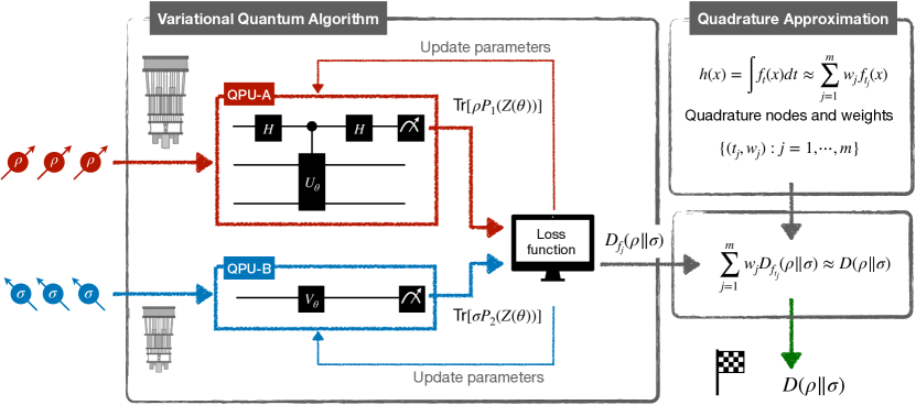
Figure 1: Estimating quantum relative entropy via variational quantum algorithm. Identical copies of the quantum states are processed (possibly across different quantum computers) through parameterized quantum circuits to extract information. The variational algorithm produces an estimate for quantum $f$-divergences, and the quantum relative entropy is then calculated as a weighted average of these $f$-divergences, based on the quadrature nodes and weights.

We validate the feasibility and effectiveness of our approach through numerical simulations, demonstrating the trainability of our parameterized quantum circuits even with basic optimizers like gradient descent. By dynamically adjusting the learning rate in response to fluctuations in the loss function during iterations, our algorithm achieves efficient convergence, yielding estimates with relative error rates around 2%. These results lay the groundwork for the future deployment of our method on quantum hardware devices.

1.2 Related works

As quantum entropies and quantum divergences play a fundamental role in quantum information science, their estimation on quantum computers has been the focus of extensive research. Several related works are summarized in Table 1.

The first class of quantum algorithms utilizes a number of independent copies of the input quantum states. [BOW19] provided two algorithms for testing the closeness of quantum states with respect to the fidelity and trace distance. [AISW20] introduced a method to compute the von Neumann entropy and quantum Rényi entropies of an $d$-dimensional quantum state with $O(d^{2}/\varepsilon^{2})$ and $O(d^{2/\alpha}/\varepsilon^{2/\alpha})$ copies, respectively. [WZW23] exploited truncated Taylor series to estimate von Neumann entropy and quantum Rényi entropies and showed that the corresponding quantum circuits can be efficiently constructed with single and two-qubit quantum gates.

Quantities	Identical copies	QSVT-based	VQA
Von Neumann entropy	[AISW20, WZW23]	[GL19, WGL+24]	[SLJ24, GPSW24]
Quantum ($\alpha$-)Rényi entropy	[AISW20, WZW23]	[SH21, WGL+24]	[GPSW24]
Quantum ($\alpha$-)Tsallis entropy	$\backslash$	[WGL+24]	$\backslash$
($\alpha$-)trace distance	[BOW19]	[WGL+24]	[CSZW21]
($\alpha$-)fidelity	[BOW19]	[WGL+24]	[CPCC20, CSZW21]
Quantum relative entropy	$\backslash$	$\backslash$	this work
Petz Rényi divergence	$\backslash$	$\backslash$	this work

Table 1: Related works of estimation methods for different quantum quantities.

The second class of algorithms involves the “purified quantum query access”, a widely adopted input model based on the general framework of quantum singular value transformation (QSVT) [GSLW19]. In this model, mixed quantum states are represented through quantum oracles that prepare their purifications. For instance, [GL19] introduced a quantum algorithm for computing von Neumann entropy with query complexity $O(d/\varepsilon^{1.5})$. Additionally, [SH21] proposed a method of computing the quantum Rényi entropy with query complexity $O\left(\frac{\kappa}{(x\varepsilon)^{2}}\log\left(\frac{d}{\varepsilon}\right)\right)$, where $\kappa>0$ satisfies $I/\kappa\leq\rho\leq I$ and $x=\operatorname{Tr}[\rho^{\alpha}]/d$. Expanding on this framework, [WGL⁺24] provided a series of new quantum algorithms that can compute quantum entropies and quantum divergences such as the quantum Rényi entropy, quantum Tsallis entropy, trace distance, and $\alpha$-fidelity for $\alpha\in(0,1)$. While the quantum relative entropy can be approached by the Sandwiched Rényi divergence in principle as $\alpha\to 1$, the latter of which can be computed from $\alpha$-fidelity using the algorithm provided in [WGL⁺24]. However, the query complexity of this approach is exponential in $1/(1-\alpha)$, which blows up as $\alpha\to 1$.

The third class of algorithms involves estimating quantum entropies using VQAs, which have proven effective for tackling problems that are challenging to solve exactly [CAB⁺21]. For instance,  [CPCC20] introduced a hybrid classical-quantum algorithm to estimate truncated fidelity. Similarly,  [CSZW21] proposed VQAs for estimating trace distance and fidelity by reformulating these tasks as optimization problems over unitary operators. Building on this,  [SLJ24] developed a variational method for estimating von Neumann entropy by expressing its variational formula as an optimization problem over parameterized quantum states. Additionally,  [GPSW24] presented a suite of VQAs for estimating von Neumann and Rényi entropies, as well as measured relative entropy and measured Rényi relative entropy, by parameterizing Hermitian operators using parameterized quantum circuits and classical neural networks.

Despite these advancements, several challenges remain. For example, [KCW21] proposed a training algorithm that minimizes over Petz-2 Rényi divergence, i.e. $\log\operatorname{Tr}[\rho^{2}\sigma^{-1}]$, with the assumption that there exists a unitary quantum channel preparing the purification of $\sigma^{-1}$. However, to the best of our knowledge, no existing approach can construct the purification of a negative exponent of an unknown quantum state without any specific structural assumptions. In summary, all current methods fail to estimate quantum relative entropy and Petz Rényi divergences from unknown quantum states due to various inherent limitations.

1.3 Organization

The remainder of this paper is organized as follows. Section 2 introduces the variational expressions of quantum relative entropy and Petz Rényi divergence. In Section 3, we propose a technique for parameterizing Hermitian polynomial operators to estimate their traces with quantum states. Building on these foundations, Section 4 presents variational quantum algorithms for $f$-divergence, quantum relative entropy, and Petz Rényi divergence. Section 5 provides an error analysis for the proposed algorithms. Section 6 shows the results of numerical simulations, and Section 7 concludes with a summary of the work and outlines open questions for future research.

2 Preliminaries

2.1 Notations

In this section, we set the notations and define several quantities that will be used throughout this work. Some frequently used notations are summarized in Table 2. We denote $\rho$ and $\sigma$ as quantum states. The logarithm function with base 2 is denoted as $\log$, and the natural logarithm (base $e$) as $\ln$. The set of integers $\{1,2,\dots,p\}$ is denoted by $[p]$. We use $\hat{x}$ to denote an estimated value of $x$.

Notations	Descriptions
$D(\rho\|\sigma)$	Quantum relative entropy
$D_{\alpha}(\rho\|\sigma)$	Petz Rényi divergence with $\alpha\in(0,1)\cup(1,2]$
$D_{f}(\rho\|\sigma)$	Standard $f$-divergence
$Q_{\alpha}(\rho\|\sigma)$	Quasi-relative entropy $\operatorname{Tr}[\rho^{\alpha}\sigma^{1-\alpha}]$
$\hat{x}$	Estimate of a quantity $x$, such as $\hat{D}$, $\hat{D}_{\alpha}$, $\hat{D}_{f}$, $\hat{Q}_{\alpha}$
$f_{t}(x)$	Function $(x-1)/(t(x-1)+1)$ with $t\in[0,1]$
$r_{m}(x)$	Quadrature approximation for $\log(x)$ with $m$ quadrature nodes
$h_{m}(x)$	Quadrature approximation for $x^{1-\alpha}$ with $m$ quadrature nodes

Table 2: Notational conventions of divergences and quadrature approximation functions.

2.2 Variational expression of quantum relative entropies

In this section, we introduce the standard $f$-divergence and its variational expression for a specific class of $f_{t}$-divergence. Then we provide the variational forms for the quantum relative entropy and Petz Rényi divergence, using the Gauss-Radau-Jacobi (GRJ) quadrature approximation. The GRJ quadrature method provides an efficient technique to approximate integrals involving weight functions of the form $(1-t)^{a}(1+t)^{b}$ by discretizing the integral into a weighted sum over carefully chosen quadrature nodes. Leveraging the linearity of the standard $f$-divergence with respect to $f$, we can reformulate the integral representations of quantum relative entropy and Petz Rényi divergence as summations of $f_{t}$-divergences, enabling these quantities to be effectively estimated within the variational framework.

2.2.1 Standard $f$-divergence

The definition of standard $f$-divergence is as follows [Pet86, HM17]:

Definition 1 (Standard $f$-divergence).

Let $\rho$, $\sigma$ be positive semidefinite operators on ${\cal H}$ with spectral decompositions $\rho=\sum_{j}\eta_{j}P_{j}$ and $\sigma=\sum_{k}\mu_{k}Q_{k}$. The standard $f$-divergence is defined by

$$D_{f}(\rho\|\sigma)\mathrel{\mathop{\mathchar 12346\relax}}=\sum_{j\mathrel{\mathop{\mathchar 12346\relax}}\eta_{j}>0}\sum_{k\mathrel{\mathop{\mathchar 12346\relax}}\mu_{k}>0}\eta_{j}f(\mu_{k}\eta_{j}^{-1})\operatorname{Tr}[P_{j}Q_{k}]+f(0^{+})\operatorname{Tr}[\rho(I-\sigma^{0})],$$ (1)

where $\sigma^{0}$ denotes the projector onto the support of $\sigma$.

Note that for quantum states $\rho$ and $\sigma$ that satisfy ${\operatorname{supp}}(\rho)\subseteq{\operatorname{supp}}(\sigma)$, the second term in Eq. (1) vanishes since $\operatorname{Tr}[\rho(I-\sigma^{0})]=0$. When we set the function $f$ in the definition above as

$$f_{t}(x)\mathrel{\mathop{\mathchar 12346\relax}}=\frac{x-1}{t(x-1)+1}~~\text{for }t\in[0,1],$$ (2)

its corresponding standard divergence $D_{f_{t}}(\rho\|\sigma)$ has a variational expression established in [BFF24].

Lemma 2 ([BFF24]).

Let $\rho$ and $\sigma$ be positive semidefinite operators on a finite-dimensional Hilbert space ${\cal H}$. Then

$$D_{f_{t}}(\rho\|\sigma)= \inf_{Z}\frac{1}{t}\left\{\operatorname{Tr}[\rho]+\operatorname{Tr}[\rho(Z+Z^{\dagger})]+(1-t)\operatorname{Tr}[\rho Z^{\dagger}Z]+t\operatorname{Tr}[\sigma ZZ^{\dagger}]\right\},$$ (3)

where the infimum on the right-hand side is taken over all bounded linear operators $Z$ on ${\cal H}$.

Based on the lemma above, quantum relative entropy and Petz Rényi divergence can be represented by variational expressions.

2.2.2 Quantum relative entropy

Let $\rho$ and $\sigma$ be two quantum states. Their quantum relative entropy is defined as [Ume62]

$$D(\rho\|\sigma)\mathrel{\mathop{\mathchar 12346\relax}}=\operatorname{Tr}[\rho(\log\rho-\log\sigma)],$$ (4)

if ${\operatorname{supp}}(\rho)\subseteq{\operatorname{supp}}(\sigma)$ and $+\infty$ otherwise. In particular, let $f(x)=-\log(x)$. The corresponding standard $f$-divergence simplifies to the quantum relative entropy,

$$D_{-\log}(\rho\|\sigma)=D(\rho\|\sigma).$$ (5)

With the integral representation of logarithm, $\ln(x)=\int_{0}^{1}f_{t}(x)\mathrm{d}t$, we can approximate the logarithm using GRJ quadrature as follows [BFF24, Theorem 3.8],

$$\log(x)\approx r_{m}(x)\mathrel{\mathop{\mathchar 12346\relax}}=\frac{1}{\ln 2}\sum_{j=1}^{m}w_{j}f_{t_{j}}(x),$$ (6)

where $\{t_{j}\}_{j=1}^{m}$ is the set of GRJ quadrature nodes with a fixed node $t_{m}=1$, and $\{w_{j}\}_{j=1}^{m}$ are corresponding weights. The quadrature approximation for $\log x$ is shown in Figure 2 (a), which converges to the exact value as the number of quadrature nodes $m$ increases. Combining Eqs. (5) and (6), we obtain the approximation of quantum relative entropy as follows:

$$D(\rho\|\sigma)\approx D_{-r_{m}}(\rho\|\sigma)=-\sum_{j=1}^{m}\frac{w_{j}}{\ln 2}D_{f_{t_{j}}}(\rho\|\sigma)$$ (7)

where each $D_{f_{t_{j}}}(\rho\|\sigma)$ on the right-hand side can be evaluated using the variational expression provided in Lemma 2.

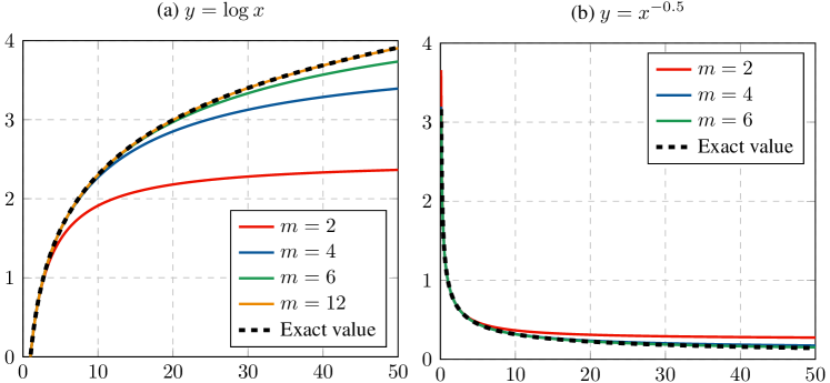
Figure 2: Performance of GRJ quadrature approximation. (a) Quadrature approximation for the function $y=\log x$; (b) Quadrature approximation for the function $y=x^{-0.5}$. The approximation converges to the exact value as the number of quadrature nodes $m$ increases.

2.2.3 Petz Rényi divergence

Let $\rho$ and $\sigma$ be two quantum states. The Petz Rényi divergence is defined as [Pet86]

$$D_{\alpha}(\rho\|\sigma)\mathrel{\mathop{\mathchar 12346\relax}}=\frac{1}{\alpha-1}\log Q_{\alpha}(\rho\|\sigma),$$ (8)

if ${\operatorname{supp}}(\rho)\subseteq{\operatorname{supp}}(\sigma)$ and $+\infty$ otherwise. Here $Q_{\alpha}(\rho\|\sigma)\mathrel{\mathop{\mathchar 12346\relax}}=\operatorname{Tr}[\rho^{\alpha}\sigma^{1-\alpha}]$ is the quasi-relative entropy, and we focus on $\alpha\in(0,1)\cup(1,2]$ which is the range of particular interest. Let $f(x)=x^{1-\alpha}$. The corresponding standard $f$-divergence reduces to

$$D_{x^{1-\alpha}}(\rho\|\sigma)=Q_{\alpha}(\rho\|\sigma).$$ (9)

To implement the quadrature approximation, an integral representation for the power function is required, which is provided by the Löwner’s Theorem [Löw34], for $\alpha\in(0,1)\cup(1,2)$,

$$x^{1-\alpha}-1=\frac{\sin(\alpha\pi)}{\pi}\int_{0}^{1}f_{t}(x)t^{\alpha-1}(1-t)^{1-\alpha}\mathrm{d}t.$$ (10)

The integral on the right-hand side can be approximated via GRJ quadratures by [FF23, Theorem 1] or [HTB24, Proposition 3.12],

$$\sum_{j=1}^{m}w_{j}f_{t_{j}}(x)\leq\int_{0}^{1}f_{t}(x) t^{\alpha-1}(1-t)^{1-\alpha}\mathrm{d}t\leq\sum_{j=1}^{m}\bar{w}_{j}f_{\bar{t}_{j}}(x).$$ (11)

Here, $\{\bar{t}_{j}\}_{j=1}^{m}$ and $\{\bar{w}_{j}\}_{j=1}^{m}$ represent the nodes and weights of the GRJ quadrature with a fixed node at $\bar{t}_{1}=0$, while $\{t_{j}\}_{j=1}^{m}$ and $\{w_{j}\}_{j=1}^{m}$ correspond to the nodes and weights of the GRJ quadrature with a fixed node at $t_{m}=1$. Furthermore, as $m\to\infty$, both bounds converge to the exact value of the integral. Therefore, the integral in Eq. (11) can be approximated using either the upper bound or the lower bound. In the following discussion, we focus on the lower bound without loss of generality.

Combining Eqs. (10) and (11), we have

$$x^{1-\alpha} \approx h_{m}(x)\mathrel{\mathop{\mathchar 12346\relax}}=1+\frac{\sin(\alpha\pi)}{\pi}\sum_{j=1}^{m}w_{j}f_{t_{j}}(x).$$

The performance of this quadrature approximation is shown in Figure 2 (b), where we take $\alpha=1.5$ as an example. As given in Eq. (9), we have the approximation to $Q_{\alpha}(\rho\|\sigma)$ by

$$Q_{\alpha}(\rho\|\sigma)\approx D_{h_{m}}(\rho\|\sigma)=1+\frac{\sin(\alpha\pi)}{\pi}\sum_{j=1}^{m}w_{j}D_{f_{t_{j}}}(\rho\|\sigma),$$ (12)

where each $D_{f_{t_{j}}}(\rho\|\sigma)$ on the right-hand side can be evaluated using the variational expression provided in Lemma 2.

In the case of $\alpha=2$, we can consider $t=1$ and the standard $f$-divergence gives [BFF24, Remark 3.6] the following relation,

$$Q_{2}(\rho\|\sigma) =1-D_{f_{1}}(\rho\|\sigma)~~\text{and}~~D_{2}(\rho\|\sigma)=\log Q_{2}(\rho\|\sigma).$$ (13)

3 Parameterization of Hermitian polynomial operators

The variational expression mentioned in the previous section can be generalized to the following optimization problem:

$$\inf_{\{Z_{1},\dots,Z_{N}\}}\left\{\operatorname{Tr}[\rho P(Z_{1},\dots,Z_{N})]+\operatorname{Tr}[\sigma Q(Z_{1},\dots,Z_{N})]\right\},$$ (14)

where $\{Z_{1},Z_{2},\dots,Z_{N}\}$ is a set of linear operators, $P$ and $Q$ are two Hermitian polynomials that satisfy $P^{\dagger}=P$ and $Q^{\dagger}=Q$. In this section, we provide a method to parameterize the polynomial observables $P$ and $Q$, and a sampling procedure to estimate $\operatorname{Tr}[\rho P]$ and $\operatorname{Tr}[\sigma Q]$ that lands well on quantum computers.

Our method is based on the singular value decomposition and the extended SWAP test [KCW21]. Without loss of generality, we consider the $p$-th order term in the polynomial, which takes the form

$$\sum_{\bm{i}\in[N]^{p}}a_{\bm{i}}\left({\cal Z}_{\bm{i}}+\mathcal{Z}_{\bm{i}}^{\dagger}\right),~~\text{where}~~a_{\bm{i}}\in\mathbb{R},~{\cal Z}_{\bm{i}}=\prod_{k=1}^{p}Z_{i_{k}},$$ (15)

where $\bm{i}\mathrel{\mathop{\mathchar 12346\relax}}=(i_{1},i_{2},\dots,i_{p})\in[N]^{p}$ is an index-sequence of length $p$ . To parameterize the polynomial $P(Z_{1},\dots,Z_{N})$ and estimate the value $\operatorname{Tr}[\rho P]$, it suffices to parameterize the linear operator ${\cal Z}_{\bm{i}}$ and then estimate the value $\operatorname{Tr}[\rho({\cal Z}_{\bm{i}}+{\cal Z}_{\bm{i}}^{\dagger})]$. Detailed procedures are given as follows.

Parameterization. With singular value decomposition, a linear operator can be parameterized by

$$Z_{i_{k}}=\sum_{j_{k}=1}^{d}\lambda_{k,j_{k}}U_{i_{k}}|j_{k}\rangle\langle j_{k}|V_{i_{k}},$$

where $\lambda_{k,j_{k}}\geq 0$ and $\{|1\rangle,|2\rangle,\dots,|d\rangle\}$ denotes a set of computational basis. Then we have

$${\cal Z}_{\bm{i}} =\sum_{(j_{1},\dots,j_{p})\in[d]^{p}}\prod_{k=1}^{p}\lambda_{k,j_{k}}U_{i_{k}}|j_{k}\rangle\langle j_{k}|V_{i_{k}}.$$ (16)

We parameterize the unitaries $U_{i_{k}}$ and $V_{i_{k}}$ with a set of parameterized quantum circuits $U_{i_{k}}(\bm{\theta}_{i_{k}})$ and $V_{i_{k}}(\bm{\beta}_{i_{k}})$, where the circuit structures are tailored to the specific problems being addressed and the available quantum hardware. The dimensions of vectors $\bm{\theta}_{i_{k}}$ and $\bm{\beta}_{i_{k}}$ depend on the structure of the parameterized quantum circuits.

When the linear operators $Z_{i}$ are bounded, Eq. (14) transforms into a constrained optimization problem, expressed as $0\leq\|Z_{i}\|\leq M_{i}$ for all $i$, where $\|\cdot\|$ denotes a suitable operator norm and $M_{i}$ are given constants. This optimization can be efficiently handled by imposing constraints on the parameters $\lambda_{k,j_{k}}$ during data processing on classical computers. Moreover, an alternative approach for parameterizing a linear operator, which involves incorporating classical neural networks (CNNs) as used in [GPSW24], is detailed in Appendix A.

Sampling. Denote $\bm{j}\mathrel{\mathop{\mathchar 12346\relax}}=(j_{1},j_{2}\dots,j_{p})\in[d]^{p}$, $a_{\bm{j}}\mathrel{\mathop{\mathchar 12346\relax}}=\prod_{k=1}^{p}\lambda_{k,j_{k}}$, and

$$\Theta_{\bm{j},\bm{i}}\mathrel{\mathop{\mathchar 12346\relax}}=\mathrm{Re}\left[\operatorname{Tr}\left(\rho\prod_{k=1}^{p}U_{i_{k}}|j_{k}\rangle\langle j_{k}|V_{i_{k}}\right)\right].$$ (17)

Due to Eq. (16), after parameterization, the quantity we need to estimate becomes

$$\operatorname{Tr}[\rho({\cal Z}_{\bm{i}}+{\cal Z}_{\bm{i}}^{\dagger})] =2\mathrm{Re}\operatorname{Tr}[\rho{\cal Z}_{\bm{i}}]=2\sum_{\bm{j}\in[d]^{p}}a_{\bm{j}}\Theta_{\bm{j},\bm{i}}.$$

We can estimate the quantity above based on the extended SWAP test provided in [KCW21, Theorem 2.3], as adapted in the following lemma.

Lemma 3.

Let $\rho$ be a quantum state of dimension $d$, and ${\cal Z}_{\bm{i}}$ be the linear operator defined in Eq. (15), the corresponding parameterization of which is Eq. (16). Denote $\bm{j}=(j_{1},j_{2},\dots,j_{p})\in[d]^{p}$ and $|\bm{j}\rangle=|j_{1}\rangle|j_{2}\rangle\cdots|j_{p}\rangle$. Then the unitary circuit $\chi_{\bm{i}}$ shown in Figure 3 gives

$$\Theta_{\bm{j},\bm{i}}=2\operatorname{Tr}\left[\left(|0\rangle\langle 0|\otimes I\right)\chi_{\bm{i}}\left(|0\rangle\langle 0|\otimes\rho\otimes|\bm{j}\rangle\langle\bm{j}|\right)\chi_{\bm{i}}^{\dagger}\right]-1.$$

More specifically, the unitary operation $\chi_{\bm{i}}$ consists of two Hadamard gates, a series of controlled unitaries, and controlled cyclic permutation. We implement the unitary $\chi_{\bm{i}}$ on the input state $|0\rangle\langle 0|\otimes\rho\otimes|\bm{j}\rangle\langle\bm{j}|$, and then measure the first qubit. The probability of outcome $0$ of the measurement is given by $(\Theta_{\bm{j},\bm{i}}+1)/2$.

Figure 3: Visualization of unitary operation $\chi_{\bm{i}}$. We evolve the input state $|0\rangle\langle 0|\otimes\rho\otimes|\bm{j}\rangle\langle\bm{j}|$ with a unitary operation $\chi_{\bm{i}}$, and then measure the first qubit in the computational basis. The probability of outcome $0$ of the measurement gives the value of $(\Theta_{\bm{j},\bm{i}}+1)/2$.

With the parameterization and sampling procedure mentioned above, we can estimate the loss function in the optimization problem Eq. (14) by sampling on quantum computers, which paves the way for estimating quantum relative entropies in the subsequent sections.

4 Variational quantum algorithms

In this section, we apply the general method introduced in Section 3 to estimate the standard $f_{t}$-divergence via variational quantum algorithms. By employing this as a subroutine, we can then estimate quantum relative entropies by utilizing the approximation from Eqs. (7) and (12).

4.1 Standard $f$-divergence

Based on the variational expression in Eq. (3), the evaluation procedure involves parameterizing the linear operator $Z$, estimating the individual terms $\operatorname{Tr}[\rho(Z+Z^{\dagger})]$, $\operatorname{Tr}[\rho Z^{\dagger}Z]$, and $\operatorname{Tr}[\sigma ZZ^{\dagger}]$, and finally optimizing the loss function. The detailed steps are as follows.

Parameterization. The first step is to parameterize the linear operator $Z$ with singular value decomposition, i.e., $Z=U\Lambda V$, where $U$ and $V$ are two unitary operators, $\Lambda$ is non-negative real diagonal matrix. We choose a set of basis $\{|i\rangle\}_{i=1}^{d}$ and parameterize $\Lambda$ as $\sum_{i=1}^{d}\lambda_{i}|i\rangle\langle i|$, where $\lambda_{i}\geq 0$ and $\lambda_{i}\in\mathbb{R}$ for all $i$. All parameters $\lambda_{i}$ are collectively represented as $\boldsymbol{\lambda}$. Then the unitaries $U$ and $V$ are represented by two parameterized quantum circuit $U(\bm{\theta})$ and $V(\bm{\beta})$ with parameters $\bm{\theta}\in\mathbb{R}^{q}$ and $\bm{\beta}\in\mathbb{R}^{r}$. For the sake of simplicity, we denote $U(\bm{\theta})$ as $U_{\bm{\theta}}$ and $V(\bm{\beta})$ as $V_{\bm{\beta}}$. Then the linear operator $Z$ is then parameterized as

$$Z=\sum_{i=1}^{d}\lambda_{i}U_{\bm{\theta}}|i\rangle\langle i|V_{\bm{\beta}}.$$

To ensure the efficiency in practice, we can parameterize $\Lambda$ with a sparse diagonal matrix that only contains at most $s$ nonzero elements, i.e., $\Lambda=\sum_{k=1}^{s}\lambda_{i_{k}}|i_{k}\rangle\langle i_{k}|$, where $i_{k}\in[d]$.

Sampling. With the above parameterization, we obtain

$$\operatorname{Tr}[\rho Z^{\dagger}Z] =\sum_{i=1}^{d}\lambda_{i}^{2}\operatorname{Tr}\left[\rho V_{\bm{\beta}}^{\dagger}|i\rangle\langle i|V_{\bm{\beta}}\right],$$

$$\operatorname{Tr}[\sigma ZZ^{\dagger}] =\sum_{i=1}^{d}\lambda_{i}^{2}\operatorname{Tr}\left[\sigma U_{\bm{\theta}}|i\rangle\langle i|U_{\bm{\theta}}^{\dagger}\right],$$

$$\operatorname{Tr}[\rho(Z+Z^{\dagger})] =4\sum_{i=1}^{d}\lambda_{i}\operatorname{Tr}\left[(|0\rangle\langle 0|\otimes I)\chi(|0\rangle\langle 0|\otimes\rho\otimes|i\rangle\langle i|)\chi^{\dagger}\right]-2,$$

where $\chi$ is a unitary operation constructed according to the quantum circuit shown in Figure 4. Then each individual term above can be estimated on quantum computers.

Figure 4: Visualization of unitary operation $\chi$. It consists of two Hadamard gates $H$, controlled $U_{\bm{\theta}}$, $V_{\bm{\beta}}$ gates, and a controlled swap gates.

More specifically, denote the probability distributions as

$$p_{\bm{\beta}}^{(i)}\mathrel{\mathop{\mathchar 12346\relax}}=\operatorname{Tr}\left[V_{\bm{\beta}}\rho V_{\bm{\beta}}^{\dagger}|i\rangle\langle i|\right],$$ (18a)

$$p_{\bm{\theta}}^{(i)}\mathrel{\mathop{\mathchar 12346\relax}}=\operatorname{Tr}\left[U^{\dagger}_{\bm{\theta}}\sigma U_{\bm{\theta}}|i\rangle\langle i|\right],$$ (18b)

$$p_{\chi}^{(i)}\mathrel{\mathop{\mathchar 12346\relax}}=\operatorname{Tr}\left[(|0\rangle\langle 0|\otimes I)\chi(|0\rangle\langle 0|\otimes\rho\otimes|i\rangle\langle i|)\chi^{\dagger}\right].$$ (18c)

Then, $p_{\bm{\theta}}^{(i)}$ can be estimated by evolving the quantum state $\sigma$ using $U^{\dagger}_{\bm{\theta}}$ and performing measurements in the computational basis. The same procedure applies to $p_{\bm{\beta}}^{(i)}$. Finally, $p_{\chi}^{(i)}$ can be estimated by evolving the initial state $|0\rangle\langle 0|\otimes\rho\otimes|i\rangle\langle i|$ with the unitary $\chi$ and measuring the first qubit in the computational basis. With these sampling results, we can obtain from classical computations that

$$\operatorname{Tr}[\rho Z^{\dagger}Z] =\sum_{i=1}^{d}\lambda_{i}^{2}p_{\bm{\beta}}^{(i)},$$

$$\operatorname{Tr}[\sigma ZZ^{\dagger}] =\sum_{i=1}^{d}\lambda_{i}^{2}p_{\bm{\theta}}^{(i)},$$

$$\operatorname{Tr}[\rho(Z+Z^{\dagger})] =4\sum_{i=1}^{d}\lambda_{i}p_{\chi}^{(i)}-2.$$

We are now well-prepared to introduce our variational quantum algorithms.

Algorithms. The idea is to solve the optimization problem defined in Eq. (3) for $m$ times to get the estimates of $D_{f_{t_{j}}}(\rho\|\sigma)$ for $j\in\{1,\cdots,m\}$, and then obtain the estimation value of $D_{-r_{m}}$ with Eq. (7) and $D_{h_{m}}(\rho\|\sigma)$ with Eq. (12), which approximate $D(\rho\|\sigma)$ and $Q_{\alpha}(\rho\|\sigma)$, respectively. In the case of $\alpha=2$, the approximation of $Q_{2}(\rho\|\sigma)$ is directly obtained by the estimation of $D_{f_{1}}(\rho\|\sigma)$. When estimating $D_{f_{t}}$, the loss function is given as follows:

$${\cal L}(\bm{\lambda},\bm{\theta},\bm{\beta})= \sum_{i=1}^{d}\left\{t\lambda_{i}^{2}p_{\bm{\theta}}^{(i)}+(1-t)\lambda_{i}^{2}p_{\bm{\beta}}^{(i)}+\lambda_{i}(4p_{\chi}^{(i)}-2)\right\}.$$ (19)

The optimization problem is thus

$$\hat{{\cal L}}=\min_{\bm{\lambda},\bm{\theta},\bm{\beta}}\mathcal{L}(\bm{\lambda},\bm{\theta},\bm{\beta}),$$ (20)

and the approximation value of $D_{f_{t}}(\rho\|\sigma)$ is

$$\hat{D}_{f_{t}}(\rho\|\sigma)=\frac{1}{t}(1+\hat{{\cal L}}).$$

We utilize the gradient descent algorithm to optimize the loss function defined by Eq. (19), which requires the gradients of the loss function with respect to each parameter. The gradients with respect to $\{\lambda_{i}\}_{i=1}^{d}$ can be computed directly on classical computers, i.e.,

$$\frac{\partial{\cal L}}{\partial\lambda_{i}}=2t\lambda_{i}p_{\bm{\theta}}^{(i)}+2(1-t)\lambda_{i}p_{\bm{\beta}}^{(i)}+(4p_{\chi}^{(i)}-2),$$ (21)

where $p_{\bm{\theta}}^{(i)}$, $p_{\bm{\beta}}^{(i)}$, and $p_{\bm{\chi}}^{(i)}$ are estimated by sampling on quantum computers. The quantum circuit parameters $\bm{\theta}$ and $\bm{\beta}$ are updated with respect to the parameter-shift rule [SBG⁺19]. The pseudocode of the algorithm for estimating $D_{f_{t}}$ is shown in Algorithm 1.

Input:

$K$	number of iterations
$\ell_{r}$	learning rate
$N$	number of samples
$t$	function parameter
$\rho$, $\sigma$	quantum states

1

Output:

$\hat{D}_{f_{t}}(\rho\|\sigma)$

estimate of $D_{f_{t}}(\rho\|\sigma)$

2

3$\bm{\lambda}^{1}\leftarrow$ Random initialization in $\mathbb{R}^{d}$.

4$\bm{\theta}^{1}\leftarrow$ Random initialization in $[0,2\pi]^{q}$.

5$\bm{\beta}^{1}\leftarrow$ Random initialization in $[0,2\pi]^{r}$.

6foreach $k\in\{1,2,\ldots,K\}$ do

7   

8   Evaluate $p_{\bm{\theta}}^{(i)}$, $p_{\bm{\beta}}^{(i)}$ and $p_{\chi}^{(i)}$ for $i=1,\dots,d$, with $\bm{\theta}^{k}$ and $\bm{\beta}^{k}$ on quantum computers.

9   Evaluate $\nabla_{\bm{\theta}}{\cal L}$ and $\nabla_{\bm{\beta}}{\cal L}$ using the parameter shift rule and compute $\nabla_{\bm{\lambda}}{\cal L}$.

10   $\bm{\theta}^{k+1}\leftarrow\bm{\theta}^{k}+\ell_{r}\nabla_{\bm{\theta}}{\cal L}$

11   $\bm{\beta}^{k+1}\leftarrow\bm{\beta}^{k}+\ell_{r}\nabla_{\bm{\beta}}{\cal L}$

12    $\bm{\lambda}^{k+1}\leftarrow\bm{\lambda}^{k}+\ell_{r}\nabla_{\bm{\lambda}}{\cal L}$

13 end foreach

14

15$\hat{\mathcal{L}}\leftarrow\mathcal{L}({\bm{\lambda}}^{K+1},{\bm{\theta}}^{K+1},{\bm{\beta}}^{K+1})$.

return $\hat{D}_{f_{t}}(\rho\|\sigma)\leftarrow(1+\hat{\cal L})/t$

Algorithm 1 Variational quantum algorithm for estimating standard $f_{t}$-divergence

It is worth noting that the only step requiring quantum computers is obtaining the sampling results $p_{\bm{\theta}}^{(i)}$, $p_{\bm{\beta}}^{(i)}$ and $p_{\chi}^{(i)}$. All other computations can be performed on classical computers. Moreover, the quantum part is well-suited for distributed scenarios. According to Eq. (18), the probability distributions $p_{\bm{\theta}}^{(i)}$ and $p_{\chi}^{(i)}$ can be sampled on a quantum computer generating the quantum state $\rho$, while $p_{\bm{\beta}}^{(i)}$ can be obtained on the quantum computer generating $\sigma$. This approach aligns well with settings that require comparing the distinguishability of quantum data generated by two distributed quantum computers, such as in cross-platform verification scenarios discussed in [EVvB⁺20, GDR⁺21, KMC23, ZYW24].

4.2 Quantum relative entropy

Recall that the approximation of quantum relative entropy is given by

$$\hat{D}(\rho\|\sigma)\approx\hat{D}_{-r_{m}}(\rho\|\sigma)=-\sum_{j=1}^{m}\frac{w_{j}}{\ln 2}\hat{D}_{f_{t_{j}}}(\rho\|\sigma),$$

where $\{t_{j}\}_{j=1}^{m}$ is the set of GRJ quadrature nodes with fixed node $t_{m}=1$. Based on Algorithm 1, the algorithm for evaluating quantum relative entropy is shown in Algorithm 2.

4.3 Petz Rényi divergence

Recall that the approximation of $Q_{\alpha}(\rho\|\sigma)$ is given by

$$\hat{Q}_{\alpha}(\rho\|\sigma)\approx\hat{D}_{h_{m}}(\rho\|\sigma)=1+\frac{\sin(\alpha\pi)}{\pi}\sum_{j=1}^{m}w_{j}\hat{D}_{f_{t_{j}}}(\rho\|\sigma),$$

where $\{t_{j}\}_{j=1}^{m}$ is the set of GRJ quadrature nodes with fixed node $t_{m}=1$. We note here that the quadrature nodes for estimating $Q_{\alpha}(\rho\|\sigma)$ are different from those for estimating $D_{-r_{m}}(\rho\|\sigma)$, since they depend on the parameter $\alpha$. The approximation of $D_{\alpha}(\rho\|\sigma)$ is thus

$$\hat{D}_{\alpha}(\rho\|\sigma)=\frac{1}{\alpha-1}\log\hat{Q}_{\alpha}(\rho\|\sigma).$$

The algorithm for estimating the Petz Rényi divergence is shown in Algorithm 3. In the case of $\alpha=2$, the estimate of $Q_{2}(\rho\|\sigma)$ is obtained by

$$\hat{Q}_{2}(\rho\|\sigma)=1-\hat{D}_{f_{1}}(\rho\|\sigma),$$

and the approximation of $D_{2}(\rho\|\sigma)$ is thus $\hat{D}_{2}(\rho\|\sigma)=\log\hat{Q}_{2}(\rho\|\sigma)$, which can be obtained by running Algorithm 1 with input $t=1$.

Input:

$K$	number of iterations
$\ell_{r}$	learning rate
$N$	number of samples
$m$	number of quadrature nodes
$\{t_{j},w_{j}\}_{j=1}^{m}$	GRJ quadrature nodes and weights
$\rho$, $\sigma$	quantum states

1

Output:

$\hat{D}(\rho\|\sigma)$

estimate of $D(\rho\|\sigma)$

2

3foreach $j\in\{1,2,\ldots,m\}$ do

4    Run Algorithm 1 with inputs $K$, $\ell_{r}$, $N$, and $t=t_{j}$.

5   Save $\hat{D}_{f_{t_{j}}}(\rho\|\sigma)$.

6 end foreach

7

8$\hat{D}_{-r_{m}}(\rho\|\sigma)\leftarrow-\sum_{j=1}^{m}\frac{w_{j}}{\ln 2}\hat{D}_{f_{t_{j}}}(\rho\|\sigma)$.

return $\hat{D}(\rho\|\sigma)\leftarrow\hat{D}_{-r_{m}}(\rho\|\sigma)$

Algorithm 2 Variational quantum algorithm for estimating quantum relative entropy

Input:

$K$	number of iterations
$\ell_{r}$	learning rate
$N$	number of samples
$m$	number of quadrature nodes
$\{t_{j},w_{j}\}_{j=1}^{m}$	GRJ quadrature nodes and weights
$\rho$, $\sigma$	quantum states

1

Output:

$\hat{D}_{\alpha}(\rho\|\sigma)$

estimate of $D_{\alpha}(\rho\|\sigma)$

2

3foreach $j\in\{1,2,\ldots,m\}$ do

4    Run Algorithm 1 with inputs $K$, $\ell_{r}$, $N$, and $t=t_{j}$.

5   Save $\hat{D}_{f_{t_{j}}}(\rho\|\sigma)$.

6 end foreach

7

8$\hat{Q}_{\alpha}(\rho\|\sigma)\leftarrow 1+\frac{\sin(\alpha\pi)}{\pi}\sum_{j=1}^{m}w_{j}\hat{D}_{f_{t_{j}}}(\rho\|\sigma)$.

return $\hat{D}_{\alpha}(\rho\|\sigma)\leftarrow\frac{1}{\alpha-1}\log\hat{Q}_{\alpha}(\rho\|\sigma)$

Algorithm 3 Variational quantum algorithm for estimating Petz Rényi divergence

5 Error analysis

We provide an error analysis of our algorithm. The total error consists of two components: $\varepsilon_{Q}$, which arises from the quadrature approximation and can be reduced by increasing the number of quadrature nodes $m$; and $\varepsilon_{V}$, which results from the heuristic nature of the variational algorithms.

Proposition 4 (Error bound for estimating $D(\rho\|\sigma)$).

For any quantum states $\rho$ and $\sigma$ with their supports ${\operatorname{supp}}(\rho)\subseteq{\operatorname{supp}}(\sigma)$, if the relative error of Algorithm 1 is within $\varepsilon_{V}$, i.e.,

$$\left|\frac{\hat{D}_{f_{t_{j}}}(\rho\|\sigma)-D_{f_{t_{j}}}(\rho\|\sigma)}{D_{f_{t_{j}}}(\rho\|\sigma)}\right|\leq\varepsilon_{V},~~j=1,2,\dots,m,$$ (22)

then the relative error of Algorithm 2 can be bounded by

$$\left|\frac{\hat{D}(\rho\|\sigma)-D(\rho\|\sigma)}{D(\rho\|\sigma)}\right|\leq C\frac{1+\varepsilon_{V}}{m^{2}}+\varepsilon_{V},$$

where $C\mathrel{\mathop{\mathchar 12346\relax}}=(Q_{0}(\rho\|\sigma)+Q_{2}(\rho\|\sigma))/(D(\rho\|\sigma)\ln 2)$ and $m$ is the number of quadrature nodes.

Proof.

We start from analyzing the difference between the quadrature approximation $r_{m}(x)$ and the exact function $\log x$. According to  [FF22, Proposition 2.2], we have the following inequality,

$$g(x)\leq-\log x\leq-r_{m}(x),$$ (23)

where $g(x)=-r_{m}(x)-\frac{1}{m^{2}\ln 2}\left(\frac{1}{x}+x-2\right)$. Note that $D_{f}(\rho\|\sigma)$ is linear and monotone in $f$ for fixed positive semidefinite operator $\rho$ and $\sigma$. This implies that $D_{f}(\rho\|\sigma)\leq D_{g}(\rho\|\sigma)$ if $f(x)\leq g(x)$ for all $x\in(0,+\infty)$. Due to Eq. (23), we have $D_{g}(\rho\|\sigma)\leq D(\rho\|\sigma)\leq D_{-r_{m}}(\rho\|\sigma)$, which indicates that the difference between $D(\rho\|\sigma)$ and $D_{-r_{m}}(\rho\|\sigma)$ must be smaller than the difference between $D_{-r_{m}}(\rho\|\sigma)$ and $D_{g}(\rho\|\sigma)$. Set $f_{0}(x)=x-1$ and $f_{1}(x)=(x-1)/x$. We get the following estimation

$$D_{-r_{m}}(\rho\|\sigma)-D(\rho\|\sigma) \leq D_{-r_{m}}(\rho\|\sigma)-D_{g}(\rho\|\sigma)$$

$$=\frac{1}{m^{2}\ln 2}D_{f_{0}-f_{1}}(\rho\|\sigma)$$

$$=\frac{Q_{0}(\rho\|\sigma)+Q_{2}(\rho\|\sigma)-2}{m^{2}\ln 2}$$

$$\leq\frac{Q_{0}(\rho\|\sigma)+Q_{2}(\rho\|\sigma)}{m^{2}\ln 2}$$ (24)

where $D_{f_{0}}(\rho\|\sigma)=Q_{0}(\rho\|\sigma)-1$ and $D_{f_{1}}(\rho\|\sigma)=1-Q_{2}(\rho\|\sigma)$.

The second part of the error comes from the variational algorithm for estimating the standard $f$-divergence,

$$\left|D_{-r_{m}}(\rho\|\sigma)-\hat{D}(\rho\|\sigma)\right| =\left|\sum_{j=1}^{m}\frac{w_{j}}{\ln 2}\left(D_{f_{t_{j}}}(\rho\|\sigma)-\hat{D}_{f_{t_{j}}}(\rho\|\sigma)\right)\right|$$

$$\leq\sum_{j=1}^{m}\frac{w_{j}}{\ln 2}\varepsilon_{V}D_{f_{t_{j}}}(\rho\|\sigma)$$

$$=\varepsilon_{V}D_{-r_{m}}(\rho\|\sigma)$$

$$=\varepsilon_{V}\left(D_{-r_{m}}(\rho\|\sigma)-D(\rho\|\sigma)+D(\rho\|\sigma)\right)$$

$$\leq\varepsilon_{V}\left(\frac{Q_{0}(\rho\|\sigma)+Q_{2}(\rho\|\sigma)}{m^{2}\ln 2}+D(\rho\|\sigma)\right),$$

where the first inequality follows from Eq. (22) and $w_{j}>0$ for GRJ quadrature, the last inequality follows from Eq. (24). Then the total relative error becomes

$$\left|\frac{\hat{D}(\rho\|\sigma)-D(\rho\|\sigma)}{D(\rho\|\sigma)}\right| \leq\frac{D_{-r_{m}}(\rho\|\sigma)-D(\rho\|\sigma)+\left|D_{-r_{m}}(\rho\|\sigma)-\hat{D}(\rho\|\sigma)\right|}{D(\rho\|\sigma)}$$

$$\leq\frac{Q_{0}(\rho\|\sigma)+Q_{2}(\rho\|\sigma)}{m^{2}D(\rho\|\sigma)\ln 2}(1+\varepsilon_{V})+\varepsilon_{V},$$

which completes the proof.    $\sqcap$$\sqcup$

The above analysis similarly applies to the Petz Rényi divergence. The error $\varepsilon_{Q}$ arises from the difference between the quadrature approximation $h_{m}(x)$ and the exact function $h(x)=x^{1-\alpha}$. This difference can be bounded by using Theorem 1 and Theorem 9 from [FF23].

Lemma 5 ([FF23]).

Consider the function $h(x)=x^{1-\alpha}$, whose integral representation is $h(x)=1+\int_{0}^{1}f_{t}(x)\mathrm{d}\nu_{\alpha}(t)$, where $\alpha\in(0,1)\cup(1,2)$, $f_{t}(x)$ is defined in Eq. (2), and $\mathrm{d}\nu_{\alpha}(t)=\frac{\sin(\alpha\pi)}{\pi}t^{\alpha-1}(1-t)^{1-\alpha}\mathrm{d}t.$ Let $h_{m}(x)$ be the GRJ quadrature approximations to $h(x)$ with fixed nodes at $1$. Then for $m\geq 1$ and $x>0$, we have

$$0\leq\frac{h(x)-h_{m}(x)}{1-\alpha}\leq\alpha\nu_{\alpha,m}\frac{(x-1)^{2}}{x},$$ (25)

where $\nu_{\alpha,m}=\max\left\{\nu_{\alpha,m}^{0},\nu_{\alpha,m}^{1}\right\}$ and

$$\nu_{\alpha,m}^{0}=O\left(\frac{\Gamma(\alpha)}{m^{2\alpha}\Gamma(2-\alpha)}\right),\qquad\nu_{\alpha,m}^{1}=O\left(\frac{\Gamma(2-\alpha)}{m^{2(2-\alpha)}\Gamma(\alpha)}\right).$$

We note here that for $\alpha\in(0,1)$, $h(x)-h_{m}(x)\geq 0$; while for $\alpha\in(1,2)$, $h(x)-h_{m}(x)\leq 0$. When $m\to\infty$, $h_{m}(x)$ converges to $h(x)$.

Since we obtain the estimate of $D_{\alpha}(\rho\|\sigma)$ via $D_{\alpha}(\rho\|\sigma)=\frac{1}{\alpha-1}\log Q_{\alpha}(\rho\|\sigma)$, we first provide the error bound for estimating $Q_{\alpha}(\rho\|\sigma)$ as follows.

Lemma 6 (Error bound for estimating $Q_{\alpha}(\rho\|\sigma)$).

Let $\alpha\in(0,1)\cup(1,2)$. For any quantum states $\rho$ and $\sigma$ with ${\operatorname{supp}}(\rho)\subseteq{\operatorname{supp}}(\sigma)$, if the relative error of Algorithm 1 is within $\varepsilon_{V}$ (as defined in Eq. (22)), then the error of estimating $Q_{\alpha}(\rho\|\sigma)$ is bounded as follows:

$$\left|{Q_{\alpha}(\rho\|\sigma)}-{\hat{Q}_{\alpha}(\rho\|\sigma)}\right|\leq C_{1}\nu_{\alpha,m}(1+\varepsilon_{V})+C_{2}\varepsilon_{V},$$

where $C_{1}\mathrel{\mathop{\mathchar 12346\relax}}=2\left|\alpha(1-\alpha)\right|\cdot(Q_{2}(\rho\|\sigma)-1)$, $C_{2}\mathrel{\mathop{\mathchar 12346\relax}}=\left|Q_{\alpha}(\rho\|\sigma)-1\right|$ and $\nu_{\alpha,m}$ defined in Lemma 5.

Proof.

The total error stems from two parts, i.e., $|Q_{\alpha}(\rho\|\sigma)-\hat{Q}_{\alpha}(\rho\|\sigma)|\leq|Q_{\alpha}(\rho\|\sigma)-D_{h_{m}}(\rho\|\sigma)|+|D_{h_{m}}(\rho\|\sigma)-\hat{Q}_{\alpha}(\rho\|\sigma)|$. Since $Q_{\alpha}(\rho\|\sigma)$ generates from $x^{1-\alpha}$-divergence, the first part of the error stems from the difference between $x^{1-\alpha}$ and $h_{m}(x)$. Due to Eq. (25), we have

$$\left|D_{x^{1-\alpha}}(\rho\|\sigma)-D_{h_{m}}(\rho\|\sigma)\right|\leq \left|\alpha(1-\alpha)\right|\nu_{\alpha,m}D_{\frac{1}{x}+x-2}(\rho\|\sigma)$$

$$\leq \left|\alpha(1-\alpha)\right|\nu_{\alpha,m}\cdot(Q_{2}(\rho\|\sigma)-1),$$ (26)

where the last inequality follows from $Q_{0}(\rho\|\sigma)\leq 1$. Since the relative error of Algorithm 1 is bounded by $\varepsilon_{V}$, we have

$$\left|\hat{Q}_{\alpha}(\rho\|\sigma)-D_{h_{m}}(\rho\|\sigma)\right|= \left|\frac{\sin(\alpha\pi)}{\pi}\sum_{j=1}^{m}w_{j}\left(\hat{D}_{f_{t_{j}}}(\rho\|\sigma)-D_{f_{t_{j}}}(\rho\|\sigma)\right)\right|$$

$$\leq \left|\frac{\sin(\alpha\pi)}{\pi}\right|\sum_{j=1}^{m}w_{j}\varepsilon_{V}D_{f_{t_{j}}}(\rho\|\sigma)$$

$$= \varepsilon_{V}\left|D_{h_{m}}(\rho\|\sigma)-1\right|$$ (27)

$$\leq \varepsilon_{V}\left(\left|Q_{\alpha}(\rho\|\sigma)-1\right|+\left|\alpha(1-\alpha)\right|\nu_{\alpha,m}\left(Q_{2}(\rho\|\sigma)-1\right)\right),$$ (28)

where the last inequality follows from Eq. (26). Combining Eqs. (26) and (28), we obtain the asserted result.    $\sqcap$$\sqcup$

This lemma implies that when $m\to\infty$, the error stems from quadrature approximation vanishes as $\nu_{\alpha,m}\to 0$. It also leads to the error analysis for $D_{\alpha}(\rho\|\sigma)$ as follows.

Proposition 7 (Error bound for estimating $D_{\alpha}(\rho\|\sigma)$).

Let $\alpha\in(0,1)\cup(1,2)$. For any quantum states $\rho$ and $\sigma$ with ${\operatorname{supp}}(\rho)\subseteq{\operatorname{supp}}(\sigma)$, if the relative error of Algorithm 1 is within $\varepsilon_{V}$ (as defined in Eq. (22)), then the total relative error of Algorithm 3 can be bounded by

$$\left|\frac{D_{\alpha}(\rho\|\sigma)-\hat{D}_{\alpha}(\rho\|\sigma)}{D_{\alpha}(\rho\|\sigma)}\right|\leq O(\nu_{\alpha,m})+O\left(\varepsilon_{V}\right),$$

where $\nu_{\alpha,m}$ is defined in Lemma 5 and $m$ is the number of quadrature nodes.

Proof.

The total error for estimating the Petz Rényi divergence is bounded by two logarithmic terms, i.e.,

$$\left|D_{\alpha}(\rho\|\sigma)-\hat{D}_{\alpha}(\rho\|\sigma)\right| \leq\left|\frac{1}{\alpha-1}\log\frac{Q_{\alpha}(\rho\|\sigma)}{D_{h_{m}}(\rho\|\sigma)}\right|+\left|\frac{1}{\alpha-1}\log\frac{D_{h_{m}}(\rho\|\sigma)}{\hat{Q}_{\alpha}(\rho\|\sigma)}\right|.$$

For the ease of presentation, we bound them with the $O$ notation as follows,

$$\left|\frac{1}{\alpha-1}\log\frac{Q_{\alpha}(\rho\|\sigma)}{D_{h_{m}}(\rho\|\sigma)}\right|= O\left(\left|\frac{1}{\alpha-1}\cdot\frac{Q_{\alpha}(\rho\|\sigma)-D_{h_{m}}(\rho\|\sigma)}{Q_{\alpha}(\rho\|\sigma)}\right|\right)$$

$$\leq O\left(\alpha\nu_{\alpha,m}\frac{Q_{2}(\rho\|\sigma)-1}{Q_{\alpha}(\rho\|\sigma)}\right),$$ (29)

where the equality follows as $\log x\leq x-1$ and the inequality follows from Eq. (26). The second term can be bounded by

$$\left|\frac{1}{1-\alpha}\log\frac{D_{h_{m}}(\rho\|\sigma)}{\hat{Q}_{\alpha}(\rho\|\sigma)}\right|= \left|\frac{1}{1-\alpha}\log\left(1+\frac{\hat{Q}_{\alpha}(\rho\|\sigma)-D_{h_{m}}(\rho\|\sigma)}{D_{h_{m}}(\rho\|\sigma)}\right)\right|$$

$$= O\left(\left|\frac{\hat{Q}_{\alpha}(\rho\|\sigma)-D_{h_{m}}(\rho\|\sigma)}{(1-\alpha)D_{h_{m}}(\rho\|\sigma)}\right|\right)$$

$$\leq O\left(\varepsilon_{V}\frac{D_{h_{m}}(\rho\|\sigma)-1}{(\alpha-1)D_{h_{m}}(\rho\|\sigma)}\right)$$

$$\leq O\left(\frac{\varepsilon_{V}}{|1-\alpha|}\max\left\{1,\frac{1}{D_{h_{2}}(\rho\|\sigma)}-1\right\}\right),$$ (30)

where the first inequality follows from Eq. (27) and the second inequality follows from two properties of $D_{h_{m}}(\rho\|\sigma)$: (a) for $\alpha\in(1,2)$, $D_{h_{m}}(\rho\|\sigma)\geq 1$ and (b) for $\alpha\in(0,1)$ and $m\geq 2$, $D_{h_{m}}(\rho\|\sigma)\leq D_{h_{m+1}}(\rho\|\sigma)\leq 1$ [FF23]. Combining Eqs. (29) and (30), the total relative error can be bounded by $|D_{\alpha}(\rho\|\sigma)-\hat{D}_{\alpha}(\rho\|\sigma)|/D_{\alpha}(\rho\|\sigma)\leq O(\nu_{\alpha,m})+O\left(\varepsilon_{V}\right)$.    $\sqcap$$\sqcup$

In the case of $\alpha=2$, the error arises solely from the heuristic nature of the variational process, because the value of $Q_{2}(\rho\|\sigma)$ can be exactly determined from the value of $D_{f_{1}}(\rho\|\sigma)$ due to Eq. (13). Therefore, if the relative error of Algorithm 1 can be controlled within $\varepsilon_{V}$, the error bound for estimating $D_{2}(\rho\|\sigma)$ is given by:

$$\left|\frac{D_{2}(\rho\|\sigma)-\hat{D}_{2}(\rho\|\sigma)}{D_{2}(\rho\|\sigma)}\right| =\frac{1}{D_{2}(\rho\|\sigma)}\left|\log\left(1-D_{f_{1}}(\rho\|\sigma)\right)-\log\left(1-\hat{D}_{f_{1}}(\rho\|\sigma)\right)\right|$$

$$=\frac{1}{D_{2}(\rho\|\sigma)}\left|\log\left(1+\frac{D_{f_{1}}(\rho\|\sigma)-\hat{D}_{f_{1}}(\rho\|\sigma)}{\operatorname{Tr}[\rho^{2}\sigma^{-1}]}\right)\right|$$

$$=O\left(\frac{\left|D_{f_{1}}(\rho\|\sigma)-\hat{D}_{f_{1}}(\rho\|\sigma)\right|}{Q_{2}(\rho\|\sigma)D_{2}(\rho\|\sigma)}\right)$$

$$\leq O\left(\varepsilon_{V}\cdot\frac{Q_{2}(\rho\|\sigma)-1}{Q_{2}(\rho\|\sigma)D_{2}(\rho\|\sigma)}\right)=O\left(\varepsilon_{V}\right),$$

which is proportional to $\varepsilon_{V}$.

6 Numerical simulations

In this section, we present numerical simulations to validate the effectiveness of our variational algorithms via the PennyLane package [BIS⁺18]. We begin by outlining our methodology and parameter settings, followed by a discussion of the simulation results.

6.1 Numerical setup

Preparing input quantum states. We consider scenarios where the input states are one-qubit and two-qubit mixed states. For this, we use the interface qml.QubitStateVector from PennyLane to generate two pure quantum states $|\rho\rangle_{RS}$ and $|\sigma\rangle_{RS}$. These states effectively produce two mixed states on the marginal system $S$, that is, $\rho_{S}=\operatorname{Tr}_{R}[|\rho\rangle\langle\rho|]$ and $\sigma_{S}=\operatorname{Tr}_{R}[|\sigma\rangle\langle\sigma|]$.

Parameterized quantum circuits. Our ansatz is shown in Figure 5. For one-qubit cases, we set $U_{\bm{\theta}}$ and $V_{\bm{\beta}}$ as the generic single-qubit rotation gate $U_{3}$ in Figure 5(a). For two-qubit cases, we set $U_{\bm{\theta}}$ and $V_{\bm{\beta}}$ as the ansatz in Figure 5(b) with different parameters. We use $4$ layers of the two-qubit ansatz. To evaluate the gradient of the parameters in the parameterized quantum circuit, we utilize the function qml.gradients.param_shift in PennyLane.

(a)

(b)

Figure 5: Visualization of a single layer of our ansatz. (a) In single-qubit cases, the ansatz is a generic single-qubit rotation gate; (b) In two-qubit cases, the ansatz is constructed with three single-qubit rotation gates around each axis and a CNOT gate that generates entanglement.

Parameter setting. We estimate the values in Eq. (18) with sample means. The number of samples is set to be $10000$. The number of quadrature nodes $m$ is taken at $6$ . The learning rate $\ell_{r}$ and the number of iterations $K$ depend on specific situations. The choices of these parameters are empirical. The final loss is determined as the average of the loss values from the last $10$ iterations.

6.2 Numerical results

The numerical results of our simulations are shown in Table 3. For one-qubit simulations, we set iteration number $K$ as $300$; while for two-qubit simulations, we set $K$ as $200$. The loss of the first $100$ iterations of each case is shown in Figure 6–9. For all the cases, we set the learning rate $\ell_{r}$ as $0.1$. We choose $\alpha=1.5$ as an example for Petz Rényi divergence. We also note that the Petz-$2$ Rényi divergence $D_{2}(\rho\|\sigma)$ does not require a quadrature approximation, as it can be directly obtained from $D_{f_{1}}(\rho\|\sigma)$.

All exact and estimated values in the table are retained to four decimal places. It is easy to see that the quadrature approximates match the corresponding exact values to four decimal places and the relative errors of our estimated values are sufficiently small, most of which are within $1\%$.

Quantum Relative Entropies		Exact Value	Quadratures	Estimated Value	Relative Error
$1$-qubit cases	$D(\rho\|\sigma)$	$0.2470$	$0.2470$	$0.2455$	$0.59\%$
	$D_{1.5}(\rho\|\sigma)$	$0.3381$	$0.3381$	$0.3314$	$2.01\%$
	$D_{2}(\rho\|\sigma)$	$0.4073$	$\backslash$	$0.4096$	$0.56\%$
$2$-qubit cases	$D(\rho\|\sigma)$	$0.6585$	$0.6585$	$0.6514$	$1.07\%$
	$D_{1.5}(\rho\|\sigma)$	$0.9308$	$0.9308$	$0.9244$	$0.70\%$
	$D_{2}(\rho\|\sigma)$	$1.1430$	$\backslash$	$1.1377$	$0.46\%$

Table 3: A table of numerical results that compares exact values with their estimated values.

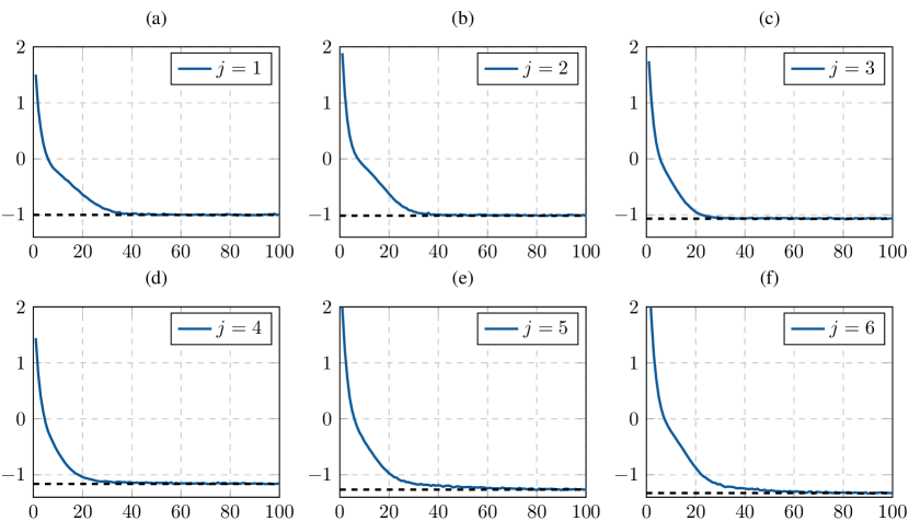
Figure 6: One-qubit case of estimating $D(\rho\|\sigma)$, where $j$ represents the index of the quadrature nodes $\{t_{j}\}_{j=1}^{6}$. The horizontal axis represents the number of iterations, and the vertical axis gives the loss value. The dashed line indicates the exact loss value, while the blue line is the loss value during training.

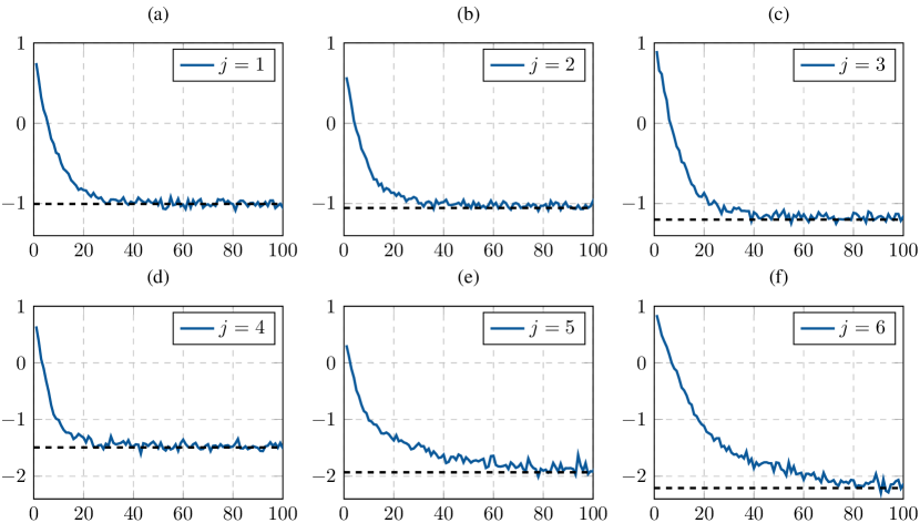
Figure 7: Two-qubit case of estimating $D(\rho\|\sigma)$, where $j$ represents the index of the quadrature nodes $\{t_{j}\}_{j=1}^{6}$. The horizontal axis represents the number of iterations, and the vertical axis gives the loss value. The dashed line indicates the exact loss value, while the blue line is the loss value during training.

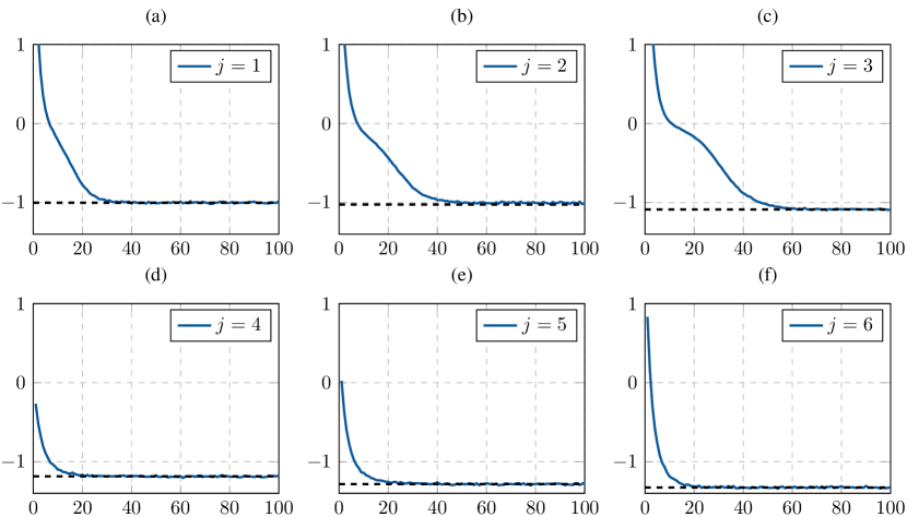
Figure 8: One-qubit case of estimating $D_{\alpha}(\rho\|\sigma)$ and $D_{2}(\rho\|\sigma)$, where $j$ represents the index of the quadrature nodes $\{t_{j}\}_{j=1}^{6}$. The horizontal axis represents the number of iterations, and the vertical axis gives the loss value. The dashed line indicates the exact loss value, while the blue line is the loss value during training. $D_{2}(\rho\|\sigma)$ is obtained with the final loss of $j=6$ as the quadrature node $t_{6}=1$.

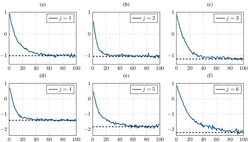
Figure 9: Two-qubit case of estimating $D_{\alpha}(\rho\|\sigma)$ and $D_{2}(\rho\|\sigma)$, where $j$ represents the index of the quadrature nodes $\{t_{j}\}_{j=1}^{6}$. The horizontal axis represents the number of iterations, and the vertical axis gives the loss value. The dashed line indicates the exact loss value, while the blue line is the loss value during training. $D_{2}(\rho\|\sigma)$ is obtained with the final loss of $j=6$ as the quadrature node $t_{6}=1$.

7 Conclusions

We have proposed a variational quantum algorithm for estimating quantum relative entropy and Petz Rényi divergence between two unknown quantum states on quantum computers, addressing open problems highlighted by Goldfeld et al. [GPSW24] and Wang et al. [WGL⁺24]. The feasibility and effectiveness of this approach were validated through theoretical analysis and numerical simulations. A notable feature of our algorithm is its applicability to distributed quantum computing scenarios, where the quantum states to be compared are hosted on cross-platform quantum devices. This capability holds promise for a wide range of potential applications in the future. Furthermore, the circuit size of our algorithm closely matches the size of the quantum states being compared, making it feasible for immediate implementation on existing quantum hardware. We leave the exploration of quantum hardware experiments as future work.

As shown in [KCW21], using the Petz-$2$ Rényi divergence as a loss function can mitigate the barren plateau problem in quantum machine learning—a significant challenge where gradients vanish exponentially with increasing circuit depth and qubit count [MBS⁺18]. Exploring whether quantum relative entropy could address this critical bottleneck in quantum machine learning offers an exciting direction for future research.

Appendix A Alternative approach to parameterizing linear operator

When parameterizing $\Lambda=\sum_{i=1}^{d}\lambda_{i}|i\rangle\langle i|$, the set of parameters $\{\lambda_{i}\}_{i=1}^{d}$ can be approximated by a classical neural network as used in [GPSW24]. More explicitly, let $y_{\bm{w}}\mathrel{\mathop{\mathchar 12346\relax}}[d]\to\mathbb{R}$ be a classical neural network with a parameter vector $\bm{w}\in\mathbb{R}^{s}$. Then we parameterize $\Lambda=\sum_{i=1}^{d}y_{\bm{w}}(i)\cdot|i\rangle\langle i|$ and the loss function becomes

$${\cal L}(\bm{w},\bm{\theta},\bm{\beta})=\sum_{i=1}^{d}\left\{ty_{\bm{w}}(i)^{2}p_{\bm{\theta}}^{(i)}+(1-t)y_{\bm{w}}(i)^{2}p_{\bm{\beta}}^{(i)}\right\}+(4p_{\chi}-2)\operatorname{Tr}[\Lambda].$$

The gradients with respect to $w_{j}$ are

$$\frac{\partial{\cal L}}{\partial w_{j}}=\sum_{i=1}^{d}\left(2ty_{\bm{w}}(i)p_{\bm{\theta}}^{(i)}+2(1-t)y_{\bm{w}}(i)p_{\bm{\beta}}^{(i)}-2\right)\frac{\partial y_{\bm{w}}(i)}{\partial w_{j}}+4\frac{\partial(p_{\chi}\operatorname{Tr}[\Lambda])}{\partial w_{j}},$$

where the gradient in the last term is estimated by central difference, i.e.,

$$\frac{\partial(p_{\chi}\operatorname{Tr}[\Lambda])}{\partial w_{j}}\approx\frac{p_{\chi}(w_{j}+\Delta w_{j})\operatorname{Tr}[\Lambda(w_{j}+\Delta w_{j})]-p_{\chi}(w_{j}-\Delta w_{j})\operatorname{Tr}[\Lambda(w_{j}-\Delta w_{j})]}{2\Delta w_{j}}.$$

Thus, the number of queries for the extended SWAP test can be reduced from $O(d)$ to $O(s)$. Moreover, if we can prepare the diagonal quantum state $\rho_{\Lambda}=\Lambda/\operatorname{Tr}[\Lambda]$ efficiently, we can estimate the following quantity with a single query of extended SWAP test,

$$\operatorname{Tr}[\rho({\cal Z}_{\bm{i}}+{\cal Z}_{\bm{i}}^{\dagger})]=\left(4\operatorname{Tr}[\left(|0\rangle\langle 0|\otimes I\right)\chi_{\bm{i}}\left(|0\rangle\langle 0|\otimes\rho\otimes\rho_{\Lambda}\right)\chi_{\bm{i}}^{\dagger}]-2\right)\cdot\operatorname{Tr}[\Lambda],$$

which directly follows by Eq. (17).

Appendix B Training with adaptive learning rate

In certain cases, a large number of quadrature nodes $m$ may be required to achieve the desired precision in the quadrature approximation. For illustration, we consider a particular $1$-qubit example that evalutes the Petz Rényi divergence between $\rho=\mathrm{diag}(0.025,0.975)$ and $\sigma=\mathrm{diag}(0.975,0.025)$ with $\alpha=1.5$. The exact value is $D_{\alpha}(\rho\|\sigma)=5.2142$, with $\operatorname{Tr}[\rho^{\alpha}\sigma^{1-\alpha}]=6.0929$. Using $m=6$ quadrature nodes yields $D_{h_{6}}=6.3508$ with a relative error of $4.23\%$. Increasing the quadrature nodes to $m=16$ significantly improves the result to $D_{h_{16}}=6.0932$, with a much smaller relative error of $4.92\times 10^{-3}\%$.

However, when estimating these quantities using our variational algorithms, we observe that as the quadrature node $t_{j}$ approaches $1$, the optimization of the loss function becomes increasingly challenging. With a constant learning rate of $\ell_{r}=0.1$, the training process succeeds for the first $12$ quadrature nodes $\{t_{j}\}_{j=1}^{12}$, but fails for the last four nodes, as shown in the left column of Figure 10. It is clear that the loss function initially converges but begins to exhibit severe fluctuations midway, eventually becoming trapped in a local minimum. This behavior suggests that an excessively large learning rate prevents the algorithm from reaching the optimal solution, necessitating the use of a smaller learning rate in such cases.

To address this, we adopt an adaptive learning rate strategy to ensure both training efficiency and accuracy. We initialize the learning rate $\ell_{r}=0.1$ and dynamically adjust this rate based on fluctuations in the loss function. Specifically, we monitor the loss values over the preceding $20$ iterations and perform a quadratic regression to measure the fluctuations using the mean square error of the regression. If the error exceeds $2$, the learning rate is halved, $\ell_{r}\leftarrow\ell_{r}/2$. As shown in the right column of Figure 10, this adaptive strategy effectively helps the algorithm escape the local minimum, ultimately achieving global convergence and giving an estimated value $5.1979$ with a relative error of $0.31\%$.

These results demonstrate that our algorithm can achieve high-precision estimations even when a large number of quadrature nodes is required. Furthermore, the convergence process could potentially be accelerated by employing more advanced optimization techniques, such as Nesterov accelerated gradient descent (NAGD), or by designing parameterized quantum circuits based on ansatzes with enhanced properties.

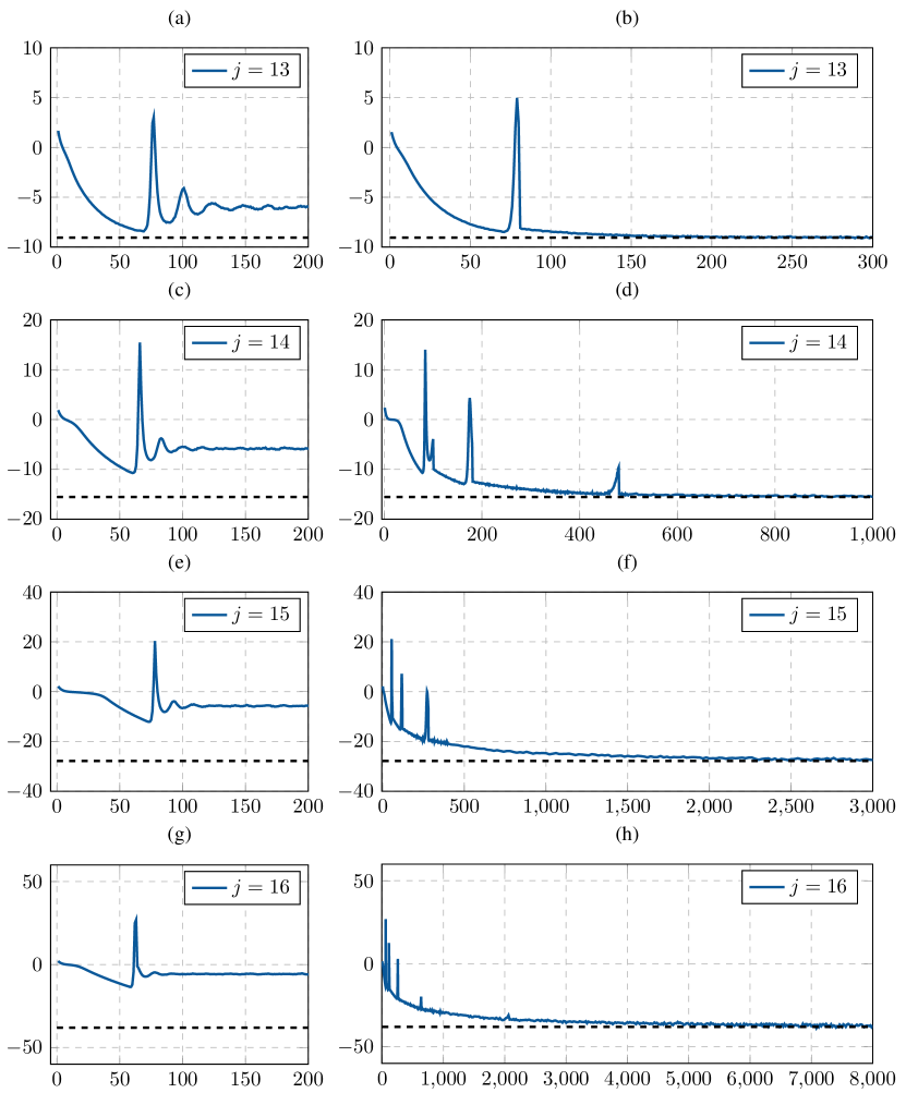
Figure 10: Training with and without adaptive learning rate. The dashed line represents the exact value of the loss, while the blue line represents the loss value during training. $j$ represents the index of the quadrature nodes. $x$-axis represents the number of iterations, while $y$-axis represents the loss value. The figures on the left show the results of the training with constant learning rate $\ell_{r}=0.1$, while those on the right show the corresponding results with adaptive learning rate.

References

- [AHS85] D. H. Ackley, G. E. Hinton, and T. J. Sejnowski. A learning algorithm for Boltzmann machines. Cognitive Science, 9(1):147–169, 1985. https://doi.org/10.1016/S0364-0213(85)80012-4.
- [AISW20] J. Acharya, I. Issa, N. V. Shende, and A. B. Wagner. Estimating quantum entropy. IEEE Journal on Selected Areas in Information Theory, 1(2):454–468, 2020. https://doi.org/10.1109/JSAIT.2020.3015235.
- [BFF24] P. Brown, H. Fawzi, and O. Fawzi. Device-independent lower bounds on the conditional von Neumann entropy. Quantum, 8:1445, 2024. https://doi.org/10.22331/q-2024-08-27-1445.
- [BIS+18] V. Bergholm, J. Izaac, M. Schuld, C. Gogolin, S. Ahmed, V. Ajith, M. S. Alam, G. Alonso-Linaje, B. AkashNarayanan, A. Asadi, et al. Pennylane: Automatic differentiation of hybrid quantum-classical computations. arXiv preprint arXiv:1811.04968, 2018. https://doi.org/10.48550/arXiv.1811.04968.
- [BOW19] C. Bădescu, R. O’Donnell, and J. Wright. Quantum state certification. In Proceedings of the 51st Annual ACM SIGACT Symposium on Theory of Computing, pages 503–514, 2019. https://doi.org/10.1145/3313276.3316344.
- [BS82] V. P. Belavkin and P. Staszewski. C*-algebraic generalization of relative entropy and entropy. In Annales de l’institut Henri Poincaré. Section A, Physique Théorique, volume 37, pages 51–58, 1982. http://www.numdam.org/item/AIHPA_1982__37_1_51_0/.
- [BWP+17] J. Biamonte, P. Wittek, N. Pancotti, P. Rebentrost, N. Wiebe, and S. Lloyd. Quantum machine learning. Nature, 549(7671):195–202, 2017. https://doi.org/10.1038/nature23474.
- [CAB+21] M. Cerezo, A. Arrasmith, R. Babbush, S. C. Benjamin, S. Endo, K. Fujii, J. R. McClean, K. Mitarai, X. Yuan, L. Cincio, et al. Variational quantum algorithms. Nature Reviews Physics, 3(9):625–644, 2021. https://doi.org/10.1038/s42254-021-00348-9.
- [CC97] N. J. Cerf and R. Cleve. Information-theoretic interpretation of quantum error-correcting codes. Physical Review A, 56(3):1721, 1997. https://doi.org/10.1103/PhysRevA.56.1721.
- [CG19] E. Chitambar and G. Gour. Quantum resource theories. Reviews of Modern Physics, 91(2):025001, 2019. https://doi.org/10.1103/RevModPhys.91.025001.
- [Cov99] T. M. Cover. Elements of information theory. John Wiley & Sons, 1999.
- [CPCC20] M. Cerezo, A. Poremba, L. Cincio, and P. J. Coles. Variational quantum fidelity estimation. Quantum, 4:248, 2020. https://doi.org/10.22331/q-2020-03-26-248.
- [Cro99] G. E. Crooks. Entropy production fluctuation theorem and the nonequilibrium work relation for free energy differences. Physical Review E, 60(3):2721, 1999. https://doi.org/10.1103/PhysRevE.60.2721.
- [CSZW21] R. Chen, Z. Song, X. Zhao, and X. Wang. Variational quantum algorithms for trace distance and fidelity estimation. Quantum Science and Technology, 7(1):015019, 2021. https://doi.org/10.1088/2058-9565/ac38ba.
- [Don86] M. J. Donald. On the relative entropy. Communications in Mathematical Physics, 105:13–34, 1986. https://doi.org/10.1007/BF01212339.
- [EVvB+20] A. Elben, B. Vermersch, R. van Bijnen, C. Kokail, T. Brydges, C. Maier, M. K. Joshi, R. Blatt, C. F. Roos, and P. Zoller. Cross-platform verification of intermediate scale quantum devices. Physical Review Letters, 124(1):010504, 2020. https://doi.org/10.1103/PhysRevLett.124.010504.
- [Fey82] R. P. Feynman. Simulating physics with computers. International Journal of Theoretical Physics, 21(6):467–488, 1982. https://doi.org/10.1007/BF02650179.
- [FF22] H. Fawzi and O. Fawzi. Semidefinite programming lower bounds on the squashed entanglement. arXiv preprint arXiv:2203.03394, 2022. https://doi.org/10.48550/arXiv.2203.03394.
- [FF23] O. Faust and H. Fawzi. Rational approximations of operator monotone and operator convex functions. arXiv preprint arXiv:2305.12405, 2023. https://doi.org/10.48550/arXiv.2305.12405.
- [GDR+21] C. Greganti, T. Demarie, M. Ringbauer, J. Jones, V. Saggio, I. A. Calafell, L. Rozema, A. Erhard, M. Meth, L. Postler, et al. Cross-verification of independent quantum devices. Physical Review X, 11(3):031049, 2021. https://doi.org/10.1103/PhysRevX.11.031049.
- [GL19] A. Gilyén and T. Li. Distributional property testing in a quantum world. arXiv preprint arXiv:1902.00814, 2019. https://doi.org/10.48550/arXiv.1902.00814.
- [GPSW24] Z. Goldfeld, D. Patel, S. Sreekumar, and M. M. Wilde. Quantum neural estimation of entropies. Physical Review A, 109(3):032431, 2024. https://doi.org/10.1103/PhysRevA.109.032431.
- [Gra11] R. M. Gray. Entropy and information theory. Springer Science & Business Media, 2011.
- [GSLW19] A. Gilyén, Y. Su, G. H. Low, and N. Wiebe. Quantum singular value transformation and beyond: exponential improvements for quantum matrix arithmetics. In Proceedings of the 51st Annual ACM SIGACT Symposium on Theory of Computing, pages 193–204, 2019. https://doi.org/10.1145/3313276.3316366.
- [Hay16] M. Hayashi. Quantum information theory. Springer, 2016. https://doi.org/10.1007/978-3-662-49725-8.
- [HM17] F. Hiai and M. Mosonyi. Different quantum -divergences and the reversibility of quantum operations. Reviews in Mathematical Physics, 29(07):1750023, 2017. https://doi.org/10.1142/S0129055X17500234.
- [HP91] F. Hiai and D. Petz. The proper formula for relative entropy and its asymptotics in quantum probability. Communications in Mathematical Physics, 143:99–114, 1991. https://doi.org/10.1007/BF02100287.
- [HTB24] T. A. Hahn, E. Y.-Z. Tan, and P. Brown. Bounds on Petz-Rényi divergences and their applications for device-independent cryptography. arXiv preprint arXiv:2408.12313, 2024. https://doi.org/10.48550/arXiv.2408.12313.
- [Jay57] E. T. Jaynes. Information theory and statistical mechanics. Physical Review, 106(4):620, 1957. https://doi.org/10.1103/PhysRev.106.620.
- [KCW21] M. Kieferova, O. M. Carlos, and N. Wiebe. Quantum generative training using Rényi divergences. arXiv preprint arXiv:2106.09567, 2021. https://doi.org/10.48550/arXiv.2106.09567.
- [KL51] S. Kullback and R. A. Leibler. On information and sufficiency. The annals of mathematical statistics, 22(1):79–86, 1951. https://www.jstor.org/stable/2236703.
- [KMC23] J. Knörzer, D. Malz, and J. I. Cirac. Cross-platform verification in quantum networks. Physical Review A, 107(6):062424, 2023. https://doi.org/10.1103/PhysRevA.107.062424.
- [KR21] M. Kliesch and I. Roth. Theory of quantum system certification. PRX quantum, 2(1):010201, 2021. https://doi.org/10.1103/PRXQuantum.2.010201.
- [Löw34] K. Löwner. Über monotone matrixfunktionen. Mathematische Zeitschrift, 38(1):177–216, 1934. https://doi.org/10.1007/BF01170633.
- [MBS+18] J. R. McClean, S. Boixo, V. N. Smelyanskiy, R. Babbush, and H. Neven. Barren plateaus in quantum neural network training landscapes. Nature Communications, 9(1):4812, 2018. https://doi.org/10.1038/s41467-018-07090-4.
- [Mur12] K. P. Murphy. Machine learning: a probabilistic perspective. MIT Press, 2012.
- [PAB+20] S. Pirandola, U. L. Andersen, L. Banchi, M. Berta, D. Bunandar, R. Colbeck, D. Englund, T. Gehring, C. Lupo, C. Ottaviani, et al. Advances in quantum cryptography. Advances in optics and photonics, 12(4):1012–1236, 2020. https://doi.org/10.1364/AOP.361502.
- [Pet86] D. Petz. Quasi-entropies for finite quantum systems. Reports on Mathematical Physics, 23(1):57–65, 1986. https://doi.org/10.1016/0034-4877(86)90067-4.
- [PR04] M. Paris and J. Rehacek. Quantum state estimation, volume 649. Springer Science & Business Media, 2004.
- [QDH+24] Y. Qian, Y. Du, Z. He, M.-H. Hsieh, and D. Tao. Multimodal deep representation learning for quantum cross-platform verification. Physical Review Letters, 133:130601, Sep 2024. https://link.aps.org/doi/10.1103/PhysRevLett.133.130601.
- [SBG+19] M. Schuld, V. Bergholm, C. Gogolin, J. Izaac, and N. Killoran. Evaluating analytic gradients on quantum hardware. Physical Review A, 99(3):032331, 2019. https://doi.org/10.1103/PhysRevA.99.032331.
- [SH21] S. Subramanian and M.-H. Hsieh. Quantum algorithm for estimating -Rényi entropies of quantum states. Physical Review A, 104(2):022428, 2021. https://doi.org/10.1103/PhysRevA.104.022428.
- [SLJ24] M. Shin, J. Lee, and K. Jeong. Estimating quantum mutual information through a quantum neural network. Quantum Information Processing, 23(2):57, 2024. https://doi.org/10.1007/s11128-023-04253-1.
- [SW02] B. Schumacher and M. D. Westmoreland. Relative entropy in quantum information theory. Contemporary Mathematics, 305:265–290, 2002.
- [Ume62] H. Umegaki. Conditional expectation in an operator algebra, IV (entropy and information). In Kodai Mathematical Seminar Reports, volume 14, pages 59–85. Department of Mathematics, Tokyo Institute of Technology, 1962. https://doi.org/10.2996/kmj/1138844604.
- [Ved02] V. Vedral. The role of relative entropy in quantum information theory. Reviews of Modern Physics, 74(1):197, 2002. https://doi.org/10.1103/RevModPhys.74.197.
- [WGL+24] Q. Wang, J. Guan, J. Liu, Z. Zhang, and M. Ying. New quantum algorithms for computing quantum entropies and distances. IEEE Transactions on Information Theory, 70(8):5653–5680, 2024. https://doi.org/10.1109/TIT.2024.3399014.
- [WZW23] Y. Wang, B. Zhao, and X. Wang. Quantum algorithms for estimating quantum entropies. Physical Review Applied, 19(4):044041, 2023. https://doi.org/10.1103/PhysRevApplied.19.044041.
- [ZYW24] C. Zheng, X. Yu, and K. Wang. Cross-platform comparison of arbitrary quantum processes. npj Quantum Information, 10(1):4, 2024. https://doi.org/10.1038/s41534-023-00797-3.