A Hybrid Framework for Reinsurance Optimization: Integrating Generative Models and Reinforcement Learning

Abstract

Reinsurance optimization is critical for insurers to manage risk exposure, ensure financial stability, and maintain solvency. Traditional approaches often struggle with dynamic claim distributions, high-dimensional constraints, and evolving market conditions. This paper introduces a novel hybrid framework that integrates Generative Models, specifically Variational Autoencoders (VAEs), with Reinforcement Learning (RL) using Proximal Policy Optimization (PPO). The framework enables dynamic and scalable optimization of reinsurance strategies by combining the generative modeling of complex claim distributions with the adaptive decision-making capabilities of reinforcement learning.

The VAE component generates synthetic claims, including rare and catastrophic events, addressing data scarcity and variability, while the PPO algorithm dynamically adjusts reinsurance parameters to maximize surplus and minimize ruin probability. The framework’s performance is validated through extensive experiments, including out-of-sample testing, stress-testing scenarios (e.g., pandemic impacts, catastrophic events), and scalability analysis across portfolio sizes. Results demonstrate its superior adaptability, scalability, and robustness compared to traditional optimization techniques, achieving higher final surpluses and computational efficiency.

Key contributions include the development of a hybrid approach for high-dimensional optimization, dynamic reinsurance parameterization, and validation against stochastic claim distributions. The proposed framework offers a transformative solution for modern reinsurance challenges, with potential applications in multi-line insurance operations, catastrophe modeling, and risk-sharing strategy design.

Keywords: Reinsurance Optimization, Generative Models, Reinforcement Learning, Variational Autoencoders (VAEs), Proximal Policy Optimization (PPO), Insurance Risk Management, Dynamic Parameter Adjustment, Stochastic Claim Modeling, Catastrophe Risk Analysis, Hybrid Computational Framework

1 Introduction

The insurance and reinsurance industries play a pivotal role in managing financial risks and ensuring economic stability. Reinsurance, which involves the transfer of risk from insurers to reinsurers, is a cornerstone of risk management strategies aimed at maintaining solvency and optimizing financial performance. However, designing effective reinsurance strategies remains a highly complex challenge due to the stochastic nature of claims, multi-dimensional constraints, and the dynamic interplay between risk retention, profitability, and regulatory compliance [4, 59].

Traditional approaches to reinsurance optimization, such as the classical Cramér-Lundberg model, have provided foundational insights into surplus dynamics and ruin probabilities. These models, while mathematically rigorous, rely on static assumptions about premium rates and claim distributions, limiting their applicability to modern reinsurance practices. Extensions to these models, including proportional and layered reinsurance structures, address some of these limitations but often remain computationally intensive and insufficiently adaptable to high-dimensional, real-world scenarios [27, 5].

In recent years, advances in machine learning and artificial intelligence (AI) have demonstrated transformative potential in addressing challenges across the insurance domain. Generative AI models, such as Variational Autoencoders (VAEs), have shown promise in capturing complex data distributions and generating synthetic data reflective of rare and catastrophic events that are underrepresented in historical datasets [42, 30]. Concurrently, reinforcement learning (RL) techniques, particularly Proximal Policy Optimization (PPO), have emerged as powerful tools for sequential decision-making and dynamic optimization in uncertain environments [61].

This paper introduces a novel hybrid framework that integrates generative AI with reinforcement learning to optimize reinsurance strategies dynamically and adaptively. By leveraging VAEs to model claim distributions and generate synthetic scenarios, the framework overcomes challenges associated with data scarcity and variability. The PPO algorithm, on the other hand, dynamically adjusts reinsurance parameters—such as retention rates and layer boundaries—based on evolving claim distributions, market conditions, and regulatory constraints. This synergy enables the framework to evaluate and optimize complex reinsurance strategies in real time, addressing high-dimensional uncertainties and ensuring financial stability [5, 16].

The proposed hybrid framework is validated through comprehensive simulations, including stress-testing scenarios such as high-frequency claims, catastrophic tail events, and pandemic-induced impacts. These evaluations demonstrate the framework’s robustness, scalability, and adaptability, significantly outperforming traditional optimization methods such as Dynamic Programming, Monte Carlo simulations, and Multi-Objective Optimization. Furthermore, sensitivity analyses and scalability tests highlight the framework’s resilience under diverse claim environments and varying portfolio sizes.

Key contributions of this work include:

1. A hybrid framework for reinsurance optimization: The integration of generative AI models (VAEs) and reinforcement learning (PPO) to address multi-dimensional, stochastic optimization challenges in reinsurance.

2. Dynamic parameterization of reinsurance strategies: Incorporation of adaptive retention rates and layer boundaries to ensure flexibility in risk-sharing mechanisms under evolving market conditions.

3. Comprehensive validation and benchmarking: Empirical evaluation against established optimization techniques, demonstrating superior performance in scalability, computational efficiency, and robustness.

The remainder of this paper is structured as follows: Section 2 presents the mathematical foundations of the surplus process, reinsurance structures, and optimization objectives. Section 3 introduces the hybrid computational framework, detailing the integration of generative AI and reinforcement learning. Section 4 describes the experimental setup, results, and benchmarking against alternative methods. Section 5 discusses the implications and limitations of the proposed framework, and Section 6 concludes with key findings and future research directions.

By bridging the gap between traditional actuarial methods and cutting-edge AI techniques, this study provides a transformative framework for reinsurance optimization, addressing pressing challenges in financial risk management and setting a foundation for future innovations in the insurance industry.

2 Model Description

This section introduces a robust and adaptable framework for modeling an insurer’s operations over a finite planning horizon, $T$. The model addresses key challenges in risk management, dynamic claim processes, and financial stability by incorporating discrete-time modeling, a generalized surplus process, and dynamic reinsurance mechanisms. This approach provides a comprehensive foundation for optimizing decision-making under uncertainty.

2.1 Discrete-Time Framework

The planning horizon $T$ is divided into $n$ discrete time intervals, denoted as $t_{1},\ldots,t_{n}$, where $t_{1}=0$ and $t_{n}=T$. Each interval represents a time step during which the insurer manages risk portfolios, generates premium income, and incurs claims. This temporal structure reflects real-world insurance practices, where financial performance and risk exposure are periodically reviewed and adjusted [4].

The discrete-time formulation enables granular evaluation of risk and financial metrics, allowing the integration of stochastic factors into operational decisions. This granularity is crucial for analyzing the dynamic interplay between claims, premiums, and reinsurance.

2.2 Modeling the Surplus Process

The financial surplus, defined as the difference between an insurer’s assets and liabilities, evolves over time based on claim occurrences and premium collections. The surplus process is modeled using an enhanced Cramér-Lundberg framework, a foundational approach in actuarial science.

Let $N_{i}$ represent the number of claims during the $i$-th interval $[t_{i-1},t_{i})$, modeled as a Poisson random variable with intensity $\lambda\Delta t_{i}$, where $\Delta t_{i}=t_{i}-t_{i-1}$. Each claim $X_{ij}$ is assumed to be independent and identically distributed (i.i.d.). The surplus process is defined as:

$$S_{i+1}=S_{i}+c\Delta t_{i}-\sum_{j=1}^{N_{i}}X_{ij},$$ (2.1)

where:

• $S_{i}$: Surplus at time $t_{i}$,

• $c$: Premium rate per unit time, calculated as:

  $$c=(1+\theta)\lambda\mathbb{E}[X],$$ (2.2)

  with $\theta>0$ representing the safety loading factor to ensure profitability and solvency [59].

This formulation provides a dynamic representation of surplus evolution, allowing for rigorous analysis of financial stability and risk mitigation strategies.

2.3 Incorporating Reinsurance Mechanisms

Reinsurance is a critical tool for risk-sharing, enabling insurers to transfer portions of their liabilities to reinsurers. This framework incorporates multiple reinsurance arrangements tailored to diverse risk profiles and operational needs.

2.3.1 Proportional Reinsurance

In proportional reinsurance, a fixed fraction $\alpha$ of each claim is retained by the insurer, with the remainder covered by the reinsurer. The surplus process is modified as:

$$S_{i+1}=S_{i}+c\Delta t_{i}-\sum_{j=1}^{N_{i}}\alpha X_{ij},$$ (2.3)

where $\alpha\in[0,1]$ represents the retention rate. This straightforward approach balances risk retention and cost efficiency [59].

2.3.2 Layered Reinsurance

Layered reinsurance divides claims into predefined layers with variable retention rates. The retained loss for a claim $X_{ij}$ is expressed as:

$$L_{ij}=\sum_{k=1}^{K}\alpha_{k}\min(\max(X_{ij}-a_{k},0),b_{k}-a_{k}),$$ (2.4)

where:

• $[a_{k},b_{k}]$: Boundaries of layer $k$,

• $\alpha_{k}$: Retention rate for layer $k$,

• $K$: Total number of layers [5].

This structure enables strategic risk-sharing, optimizing cost-effectiveness while mitigating high-severity losses.

2.3.3 Dynamic Reinsurance Adjustments

To address evolving market conditions and regulatory requirements, dynamic adjustments to retention rates and layer boundaries are incorporated:

$$\alpha_{k}(t_{i}) =\alpha_{k}^{\text{base}}+\delta_{k}(t_{i}),$$ (2.5)

$$a_{k}(t_{i}) =a_{k}^{\text{base}}+\Delta a_{k}(t_{i}),\quad b_{k}(t_{i})=b_{k}^{\text{base}}+\Delta b_{k}(t_{i}),$$ (2.6)

where $\delta_{k}(t_{i})$, $\Delta a_{k}(t_{i})$, and $\Delta b_{k}(t_{i})$ are time-dependent adjustments informed by reinforcement learning agents. These dynamic capabilities enhance the framework’s adaptability to stochastic and temporal uncertainties [62].

2.4 Optimization Objectives

The primary objective is to maximize the expected utility of the terminal surplus $S_{n}$, accounting for premiums, claims, and reinsurance costs:

$$\max_{\alpha_{k},a_{k},b_{k}}\mathbb{E}[U(S_{n})].$$ (2.7)

This optimization is subject to the following constraints:

1. Ruin Probability Constraint: The probability of financial ruin must not exceed a predefined threshold[4]:

   $$\mathbb{P}(S_{i}<0\text{ for any }i=0,\ldots,n)\leq\psi_{\text{target}}.$$ (2.8)

2. Budget Constraint: Total reinsurance premium costs must remain within a specified limit:

   $$P=\sum_{k=1}^{K}(1+\theta_{k})\beta_{k}\mathbb{E}[r_{k}(X)]\leq P_{\text{max}},$$ (2.9)

   where $\beta_{k}=1-\alpha_{k}$ and $r_{k}(X)$ represents claims covered by layer $k$ [3].

3. Layer Structure Constraint: Layer boundaries must remain non-overlapping:

   $$a_{k+1}\geq b_{k},\quad\forall k.$$ (2.10)

4. Retention Rate Bounds: Retention rates must satisfy:

   $$0\leq\alpha_{k}\leq 1,\quad\forall k.$$ (2.11)

These constraints ensure financial stability, regulatory compliance, and efficient resource allocation.

3 A Hybrid Framework for Generative Models and Reinforcement Learning in Reinsurance Optimization

The management of reinsurance portfolios requires balancing financial stability, regulatory compliance, and risk mitigation under uncertain conditions. This section introduces a hybrid framework that integrates generative AI models, specifically Variational Autoencoders (VAEs), with Reinforcement Learning (RL) using Proximal Policy Optimization (PPO). The proposed framework addresses challenges such as data scarcity, stochastic claim dynamics, and evolving market conditions by combining synthetic data generation and sequential decision-making. This hybrid approach enables adaptive and dynamic reinsurance optimization while ensuring scalability and robustness in managing diverse risk profiles.

3.1 Generative Claim Model Using Variational Autoencoders (VAE)

Variational Autoencoders (VAEs) form the generative backbone of the proposed framework, designed to model the statistical properties of historical insurance claims. VAEs address the challenge of data scarcity by generating synthetic claim scenarios that capture both observed data patterns and potential extreme events [42, 30].

3.1.1 Machine Learning Architecture and Components

The VAE architecture comprises three core components, as illustrated in Figure 1:

1. Encoder: The encoder maps high-dimensional historical claims data to a lower-dimensional latent space. This neural network extracts salient features while reducing noise, providing a probabilistic representation parameterized by mean ($\mu$) and log variance ($\log\sigma^{2}$). This latent representation ensures flexibility in modeling diverse data distributions [42].

2. Latent Space: The latent space encodes each claim as a probabilistic distribution. By sampling from this space, the VAE generates synthetic claims that extrapolate beyond the observed dataset while adhering to its statistical properties. This capability is critical for stress-testing and exploring rare, high-severity loss scenarios.

3. Decoder: The decoder reconstructs claims from the latent space, ensuring that the generated data aligns with the statistical characteristics of the historical claims. This process preserves realism while introducing controlled variability, enabling comprehensive policy testing under diverse scenarios.

Figure 1: Variational Autoencoder (VAE) architecture for generating synthetic claims. The encoder maps historical claims to a latent space, while the decoder reconstructs realistic synthetic claims [42, 33].

3.1.2 Training Objectives and Loss Function

The VAE training process balances two critical objectives:

• Reconstruction Fidelity: The reconstruction loss ensures that the decoder-generated synthetic claims closely approximate the input claims. This fidelity is quantified using the mean squared error (MSE):

  $$\mathcal{L}_{\text{reconstruction}}=\mathbb{E}\left[\|X-\hat{X}\|^{2}\right].$$

• Latent Space Regularization: The Kullback-Leibler (KL) divergence term regularizes the latent space, promoting smoothness and diversity in the generated claims:

  $$\mathcal{L}_{\text{KL}}=-\frac{1}{2}\sum\left(1+\log\sigma^{2}-\mu^{2}-\sigma^{2}\right).$$

  The overall loss function is:

  $$\mathcal{L}_{\text{VAE}}=\mathcal{L}_{\text{reconstruction}}+\beta\cdot\mathcal{L}_{\text{KL}},$$

  where $\beta$ adjusts the relative weight of the regularization term [33].

3.1.3 Application to Reinsurance Optimization

The VAE-generated synthetic claims enrich the RL training environment by introducing diverse and extreme scenarios. This expanded dataset enables the RL agent to develop robust policies that perform effectively under high-dimensional, stochastic conditions. By incorporating rare events, the framework ensures resilience against catastrophic losses and enhances decision-making in dynamic markets [16, 5].

3.2 Reinforcement Learning for Sequential Decision-Making

Reinforcement Learning (RL) is the decision-making core of the framework, optimizing reinsurance strategies through sequential learning. Built on the OpenAI Gym framework [12], the RL environment simulates realistic insurance operations, including stochastic claim dynamics, surplus evolution, and reinsurance contract adjustments.

3.2.1 State Observations and Action Space

At each timestep $t$, the RL agent observes a state vector $s_{t}$, which captures key operational metrics:

$$s_{t}=\left(S_{t},\lambda,\{\alpha_{k}\}_{k=1}^{K},\{a_{k},b_{k}\}_{k=1}^{K}\right),$$

where $S_{t}$ is the financial surplus, $\lambda$ denotes claim frequency, $\{\alpha_{k}\}$ are retention rates, and $\{a_{k},b_{k}\}$ define reinsurance layer boundaries [4, 34].

The agent adjusts these parameters by selecting actions $a_{t}$ to optimize risk-sharing and financial stability over time.

3.2.2 Reward Structure and Policy Optimization

The reward function incentivizes solvency and profitability while penalizing adverse outcomes:

$$r_{t}=\log(S_{t}+\epsilon),$$

where $\epsilon>0$ ensures numerical stability. The RL agent refines its policy $\pi(a_{t}|s_{t})$ using Proximal Policy Optimization (PPO), maximizing the cumulative discounted reward:

$$J(\pi)=\mathbb{E}_{\pi}\left[\sum_{t=0}^{T}\gamma^{t}r_{t}\right],$$

where $\gamma\in[0,1]$ balances short- and long-term objectives [61].

3.2.3 Integration with VAE-Generated Scenarios

The VAE-generated claims introduce variability and stress-test the RL agent’s policies. By exposing the agent to extreme and rare events, this integration ensures robustness in high-dimensional and uncertain environments [42, 33].

3.3 Interaction Workflow

Figure 2 illustrates the interaction between the VAE and RL components. The iterative process combines synthetic claim generation, state observation, action execution, and reward feedback to optimize reinsurance strategies dynamically.

Figure 2: Framework Overview: Interaction workflow between the VAE and RL components. The VAE generates synthetic claims, which are processed by the RL environment. The RL agent observes states, executes actions, and receives rewards to optimize reinsurance strategies dynamically.

4 Comprehensive Evaluation of Optimization Frameworks

This section presents a comprehensive evaluation of the proposed hybrid reinsurance optimization framework, focusing on simulation setup, training metrics, and benchmark performance against established methods.

4.1 Simulation Configuration and Initial Parameters

The simulation environment was designed to mimic realistic reinsurance scenarios. Table 1 summarizes the initial parameters. The insurer’s starting surplus was set at $20,000, with claims modeled using a Poisson process with an average frequency of $\lambda=10$ claims per year [51]. Claim sizes were sampled from a lognormal distribution $\mu=3.5$ and $\sigma=1.0$ [1]. These synthetic claims were used to train the Variational Autoencoder (VAE), which generated realistic scenarios for reinforcement learning.

Parameter	Value	Description
Time Horizon ($T$)	10 years	Total simulation duration
Timesteps ($n$)	200	Number of discrete time intervals
Initial Surplus ($S_{0}$)	$20,000	Starting financial surplus
Claim Frequency ($\lambda$)	10 claims/year	Modeled as a Poisson process [51]
Claim Size Distribution	Lognormal ($\mu=3.5,\sigma=1.0$)	Synthetic claims for RL training [1]
Retention Rate Bounds	$[0.2,0.5]$	Constraints on reinsurance retention rates
Reinsurance Layers ($K$)	5	Number of layers for risk sharing
Budget Limit (Budget_max)	$150,000	Maximum allowed reinsurance budget

Table 1: Initial Settings and Parameters for the Simulation

4.2 Training Metrics and Surplus Trajectory Analysis

The training metrics and surplus trajectory emphasize the PPO agent’s ability to optimize reinsurance strategies. Table 2 outlines key metrics, and Figure 3 illustrates the surplus trajectory across 6,144 timesteps.

Metric	Value
Total Timesteps	6,144
Mean Episode Reward	$-1,070$
Policy Gradient Loss	$-0.00615$
Entropy Loss	$-21.2$

Table 2: Training Metrics for the PPO Agent

Figure 3 highlights the PPO agent’s learning process. Early fluctuations reflect exploration, while stabilization over time underscores convergence to effective policies. The metrics in Table 2 provide deeper insights:

• Mean Episode Reward: A negative value of $-1,070$ indicates penalties for surplus variability and highlights the framework’s emphasis on financial stability.

• Policy Gradient Loss: The low value of $-0.00615$ demonstrates stable and consistent updates to the policy network, indicative of effective learning [61].

• Entropy Loss: A value of $-21.2$ signifies reduced randomness in decision-making as the agent transitions from exploration to exploitation [62].

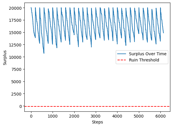
Figure 3: Surplus Trajectory Over Time. Early fluctuations diminish as the PPO agent stabilizes surplus above the ruin threshold (red dashed line).

4.3 Benchmark Performance and Comparative Analysis

The framework’s performance was benchmarked against established methods, including Dynamic Programming [6], Monte Carlo simulations [29], Hybrid Deep Monte Carlo [60], Multi-Objective Optimization [21], and Hybrid RL with Generative Models. Table 3 summarizes the results.

Method	Final Surplus ($)	Ruin Probability	Time (s)	Budget Utilization ($)	Efficiency
Dynamic Programming	12,487.71	0.0	7.96	N/A	1,568.63
Monte Carlo Simulation	12,803.21	0.0	414.27	N/A	30.91
Hybrid Deep Monte Carlo	12,973.67	0.0	411.29	N/A	31.54
Multi-Objective Optimization	12,467.12	0.0	8.52	N/A	1,462.96
Hybrid RL with Generative Models	14,280.64	0.0	7.92	259.99	1,802.60

Table 3: Benchmark Results for Reinsurance Optimization Methods

Analysis of Results:

• Dynamic Programming: Achieved a final surplus of $12,487.71 with zero ruin probability and high efficiency (1,568.63). However, its scalability is limited by the ”curse of dimensionality” [6].

• Monte Carlo Simulation: Delivered a surplus of $12,803.21 but suffered from low efficiency (30.91) due to extensive computational demands [29].

• Hybrid Deep Monte Carlo: Improved surplus ($12,973.67) but retained low efficiency (31.54), limiting its applicability for real-time optimization [60].

• Multi-Objective Optimization: Balanced performance with a surplus of $12,467.12 and strong efficiency (1,462.96). However, its static nature limits adaptability in dynamic scenarios [21].

• Hybrid RL with Generative Models: Outperformed all methods with the highest surplus ($14,280.64), strong efficiency (1,802.60), and realistic budget utilization ($259.99). Its dynamic adaptability and ability to simulate complex scenarios are key strengths [61].

The results underscore the hybrid framework’s superiority in managing high-dimensional, stochastic environments while maintaining financial stability and computational efficiency.

5 Applicability to Reinsurance Optimization

Reinsurance optimization is a complex and dynamic field that requires robust, scalable, and adaptive models to manage financial risks effectively. The hybrid framework proposed in this study integrates generative modeling and reinforcement learning to address these challenges. This section evaluates the framework’s applicability in reinsurance by analyzing its performance across different claim distributions, testing its adaptability through out-of-sample and sensitivity analyses, and examining its resilience under extreme conditions via stress testing and catastrophic event simulations. Additionally, the scalability of the framework is assessed across varying portfolio sizes to understand its limitations and potential for practical implementation in large-scale reinsurance operations.

The analysis highlights the framework’s ability to maintain surplus stability and avoid ruin under typical operational scenarios, while also identifying areas for improvement, particularly in modeling tail events and managing large portfolios. This evaluation provides valuable insights into the framework’s real-world applicability and offers directions for future enhancements.

5.1 Analysis of Generative Model Performance Across Distributions

The performance of the generative claim model was evaluated across Lognormal, Pareto, and combined Lognormal-Pareto distributions, focusing on its ability to replicate key statistical properties. Using the Kolmogorov-Smirnov (KS) test and visual comparisons, we highlight the model’s strengths in capturing central tendencies and its limitations in modeling tail behavior. Accurate tail modeling is critical for reinsurance applications due to the disproportionate impact of extreme claims [24].

5.1.1 Overall Model Performance

The KS test results indicate significant discrepancies between the training and generated datasets, with a KS statistic of $0.6264$ and a $p$-value of $0.0000$. The maximum difference location ($D$) of $14.7174$ highlights the model’s difficulty in capturing extreme claims, which dominate risk assessments in reinsurance. Figure 4 illustrates these discrepancies, showing an underrepresentation of high-severity claims in the generated data. Addressing these gaps is essential for improving the reliability of tail-event modeling.

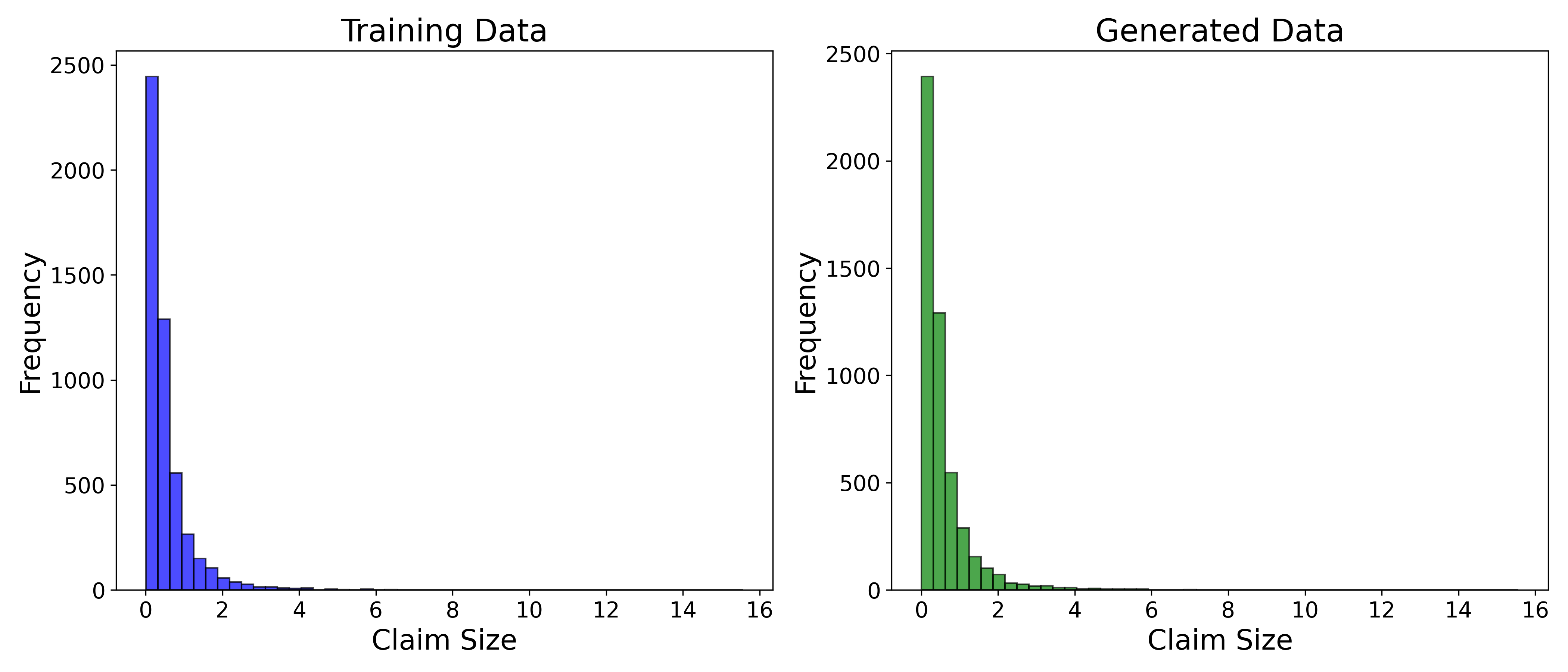
Figure 4: Comparison of Training Data and Generated Data. Discrepancies in the tail regions indicate the model’s limitations in capturing extreme events.

5.1.2 Lognormal Distribution

For the Lognormal distribution, the KS statistic of $0.5896$ and $p$-value of $0.0000$ reveal significant differences between the training and generated datasets, particularly in the tail regions. The maximum difference location ($D$) of $12.0666$ emphasizes the model’s challenges in replicating the distribution’s long-tailed nature. Figure 5 shows that while the central tendencies are accurately reproduced, large claims are underrepresented. Strategies such as tail-prioritized loss functions and data augmentation focusing on rare events may enhance the model’s performance [11].

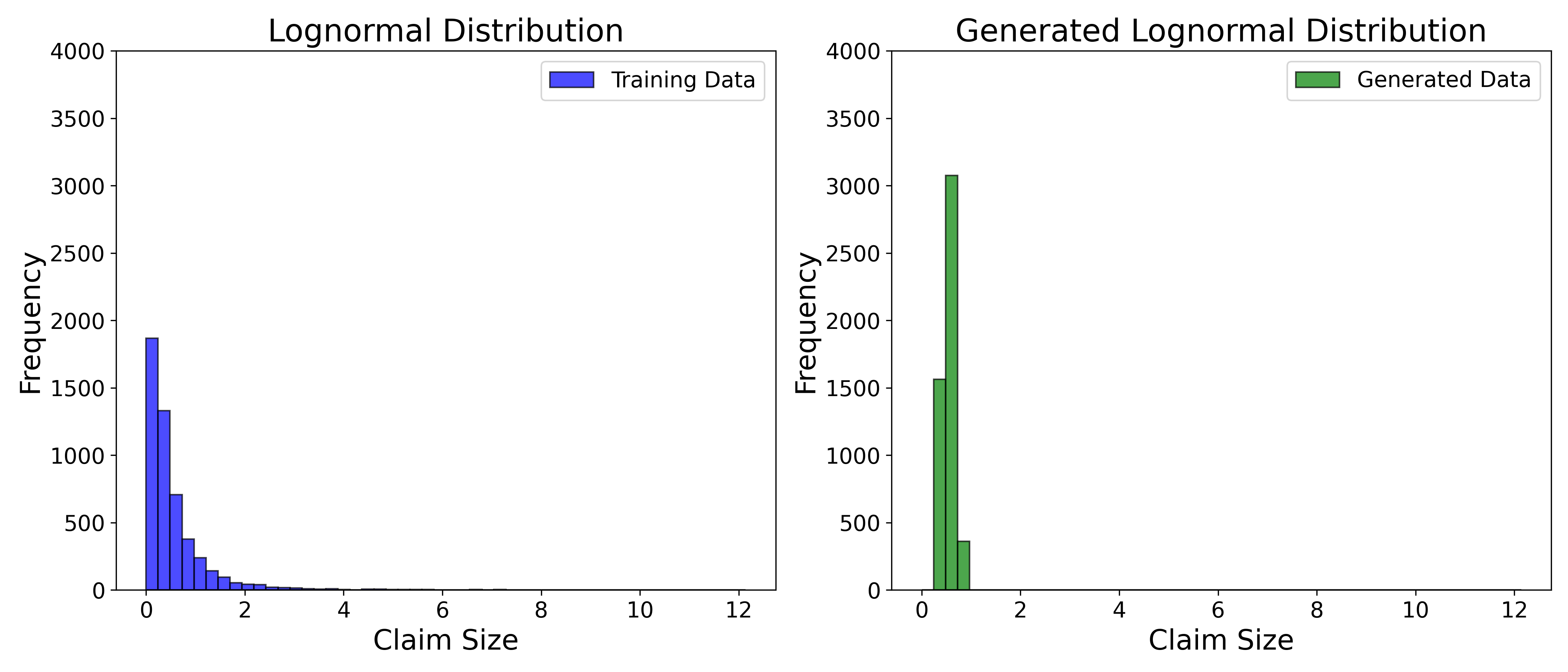
Figure 5: Training vs. Generated Data for the Lognormal Distribution. The generated data underrepresents tail regions.

5.1.3 Pareto Distribution

For the Pareto distribution, the KS test results show a statistic of $0.6230$ with a $p$-value of $0.0000$, highlighting the model’s inability to adequately represent the heavy-tailed characteristics of the data. Figure 6 reveals these limitations, particularly for rare, high-severity claims critical in reinsurance applications. Incorporating custom-tailored loss functions and oversampling the tail regions during training could mitigate these deficiencies.

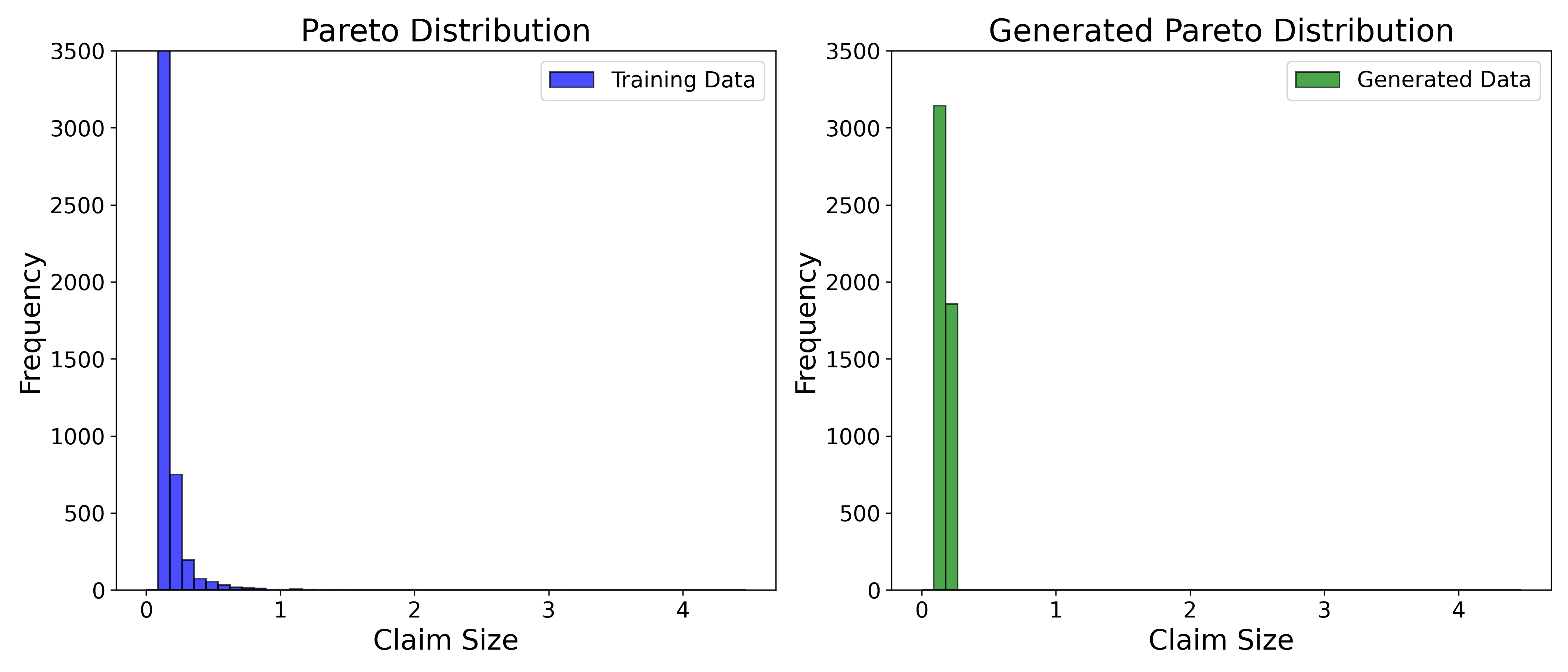
Figure 6: Training vs. Generated Data for the Pareto Distribution. The model fails to capture heavy tails accurately.

5.1.4 Combined Lognormal and Pareto Distribution

The combined Lognormal-Pareto distribution provides further insights into the model’s limitations. The KS statistic of $0.4438$ and a $p$-value of $0.0000$ confirm discrepancies in the tails, as shown in Figure 7. While the model effectively captures the central distribution characteristics, rare and extreme events are underrepresented. Increasing latent space dimensionality and introducing loss functions that prioritize tail accuracy could enhance the model’s robustness [11]. This is critical for ensuring accurate modeling in reinsurance applications, where extreme events heavily influence financial stability.

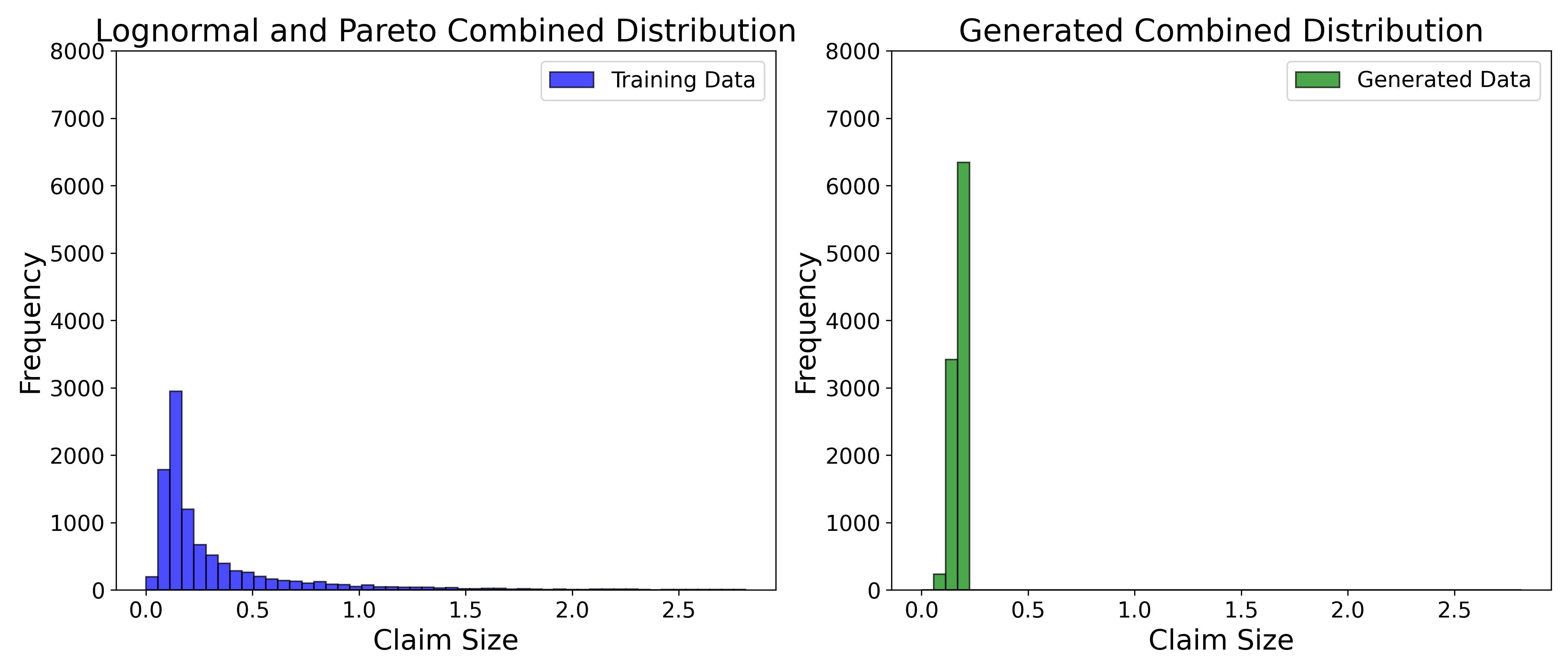
Figure 7: Training vs. Generated Data for the Combined Lognormal-Pareto Distribution. Tail discrepancies are prominent.

5.2 Out-of-Sample Performance and Sensitivity Analysis

The generative claim model’s performance was evaluated through out-of-sample testing, sensitivity analysis, and visualization of results. This comprehensive assessment highlights the model’s robustness, its ability to generalize to unseen data, and its limitations in real-world applications.

The out-of-sample testing revealed a mean surplus of $16,686.73$ with a ruin probability of $0.00\%$, demonstrating the model’s capability to effectively manage surplus over time within a simulated insurance environment. Figure 8 illustrates the surplus dynamics, where the model maintains stability without breaching the ruin threshold of $-100$. This stability indicates the model’s success in balancing premium collection and loss management under varying conditions.

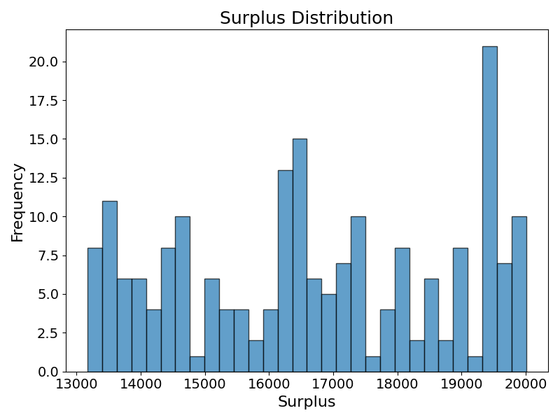
(a) Surplus Distribution. The histogram indicates stable surplus values, showcasing the model’s effective financial reserve management.

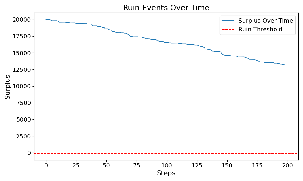
(b) Ruin Events Over Time. The surplus dynamics show no ruin events during the simulation, reinforcing the model’s reliability in managing financial risks.

Figure 8: Comparison of Surplus Distribution and Ruin Events Over Time. The figures demonstrate the model’s capacity to maintain financial stability and avoid ruin during the simulation period.

The claim size distribution, depicted in Figure 9, highlights the model’s ability to replicate central tendencies of the training data. However, discrepancies in the tail regions suggest the need for further refinement to accurately capture extreme events. Tail modeling is critical for reinsurance applications, where rare, high-severity claims significantly impact risk management and solvency assessments [24].

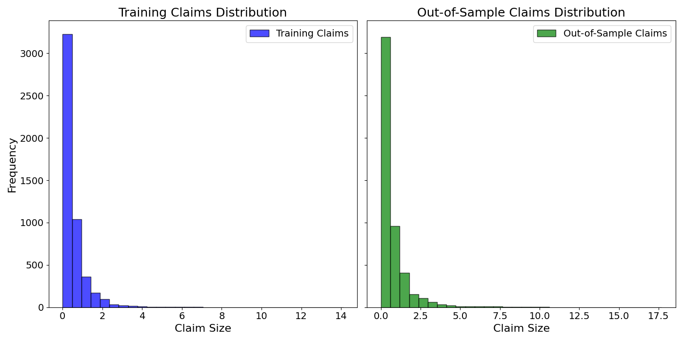
Figure 9: Claim Size Distribution. The comparison between training and out-of-sample claims reveals effective modeling of central tendencies but highlights discrepancies in tail regions.

Sensitivity analysis further evaluated the model’s robustness under varying out-of-sample conditions. When claim size distribution parameters were altered ($\mu=3.6,\sigma=1.1$), the mean surplus slightly decreased to $16,009.44$, maintaining a ruin probability of $0.00\%$. With further variations ($\mu=3.7,\sigma=1.2$), the model demonstrated adaptability, achieving a higher mean surplus of $17,052.60$. These results, summarized in Table 4, confirm the model’s resilience to changes in claim size distributions.

$\mu$	$\sigma$	Mean Surplus	Ruin Probability
3.6	1.1	16,009.44	0.00%
3.6	1.2	16,470.80	0.00%
3.7	1.0	15,211.12	0.00%
3.7	1.1	15,821.58	0.00%
3.7	1.2	17,052.60	0.00%

Table 4: Sensitivity Analysis Results for Varying $\mu$ and $\sigma$. The model exhibits consistent performance across different parameter settings, maintaining stability and low ruin probabilities.

6 Conclusion and Future Work

The proposed hybrid framework integrating generative models and reinforcement learning represents a significant advancement in the field of reinsurance optimization. By combining Variational Autoencoders (VAEs) [42] for modeling claim distributions with Proximal Policy Optimization (PPO) [61] for dynamically adjusting reinsurance strategies, the framework effectively addresses key challenges in managing high-dimensional and stochastic claim environments. The experimental results demonstrate the framework’s robustness under typical operational scenarios, its adaptability to evolving claim distributions, and its scalability across varying portfolio sizes.

The framework’s capability to manage financial stability and minimize ruin probability was evident through out-of-sample testing and sensitivity analyses. It consistently maintained surplus stability under moderate stress conditions and adapted to diverse claim distributions, underscoring its potential for real-world applications [4, 20]. Stress-testing scenarios—including high-frequency claims, pandemic-like conditions, and catastrophic events—highlighted the framework’s strengths in handling typical claims and short-term financial shocks. However, its limitations became apparent under sustained catastrophic events, underscoring the need for tailored reinsurance structures and dynamic premium adjustments [24, 5].

The scalability analysis further revealed the framework’s challenges in managing larger portfolios. While the model performed robustly for smaller portfolios, its ability to sustain surplus diminished with increasing portfolio sizes due to amplified risk exposure. These findings emphasize the importance of adaptive reinsurance strategies and risk-sharing mechanisms to ensure scalability and financial stability [59].

Despite the promising outcomes, the framework faces limitations in modeling extreme tail events—an essential aspect of reinsurance applications. Discrepancies in tail regions of the generative model outputs suggest the need for refinements. Potential improvements include the development of custom loss functions that prioritize tail accuracy [33], oversampling techniques, and enhanced latent space representations [11]. Additionally, integrating advanced optimization techniques, such as dynamic parameter tuning and multi-agent reinforcement learning, could further enhance the framework’s adaptability and resilience [62].

Future research will focus on addressing these limitations by designing more sophisticated methods for tail modeling and extending the framework to multi-line insurance operations. Incorporating external factors such as market volatility, regulatory dynamics, and macroeconomic conditions could further enhance the framework’s real-world applicability [51, 29]. Furthermore, deploying and validating the framework on large-scale, real-world insurance datasets in real-time settings will be essential for assessing its scalability and practical relevance [21, 60].

7 Acknowledgments

We acknowledge that this work was equally contributed by Stella C. Dong and James R. Finlay, reflecting our joint effort in conceptualization, methodology development, data analysis, and manuscript preparation.

References

- [1] Aitchison, J. and Brown, J. A. C., The Lognormal Distribution, Cambridge University Press, 1957.
- [2] Asmussen, S., Ruin Probabilities, World Scientific, 2000.
- [3] Avanzi, B., “Strategies for dividend distribution: A review”, North American Actuarial Journal, vol. 13, no. 2, pp. 217–251, 2009.
- [4] Asmussen, S. and Albrecher, H., Ruin Probabilities, Applications of Mathematics, vol. 14, World Scientific, 2010.
- [5] Albrecher, H., Beirlant, J., and Teugels, J. L., Reinsurance: Actuarial and Statistical Aspects, John Wiley & Sons, 2017.
- [6] Bellman, R., Dynamic Programming, Princeton University Press, 1957.
- [7] Borch, K., “The utility concept applied to the theory of insurance”, ASTIN Bulletin, vol. 1, no. 5, pp. 245–255, 1961.
- [8] Bertsekas, D. P. and Tsitsiklis, J. N., Neuro-Dynamic Programming, Athena Scientific, 1996.
- [9] Bouwer, L. M., “Have disaster losses increased due to anthropogenic climate change?”, Bulletin of the American Meteorological Society, vol. 92, no. 1, pp. 39–46, 2011.
- [10] Bertsekas, D. P., Dynamic Programming and Optimal Control, Athena Scientific, 2012.
- [11] Bengio, Y., Courville, A. and Vincent, P., “Representation learning: A review and new perspectives”, IEEE Transactions on Pattern Analysis and Machine Intelligence, vol. 35, no. 8, pp. 1798–1828, 2013.
- [12] Brockman, G., Cheung, V., Pettersson, L., et al., “OpenAI Gym”, arXiv preprint arXiv:1606.01540, 2016.
- [13] Braunsteins, P. and Mandjes, M., “The Cramér-Lundberg model with a fluctuating number of clients”, Insurance: Mathematics and Economics, 2023.
- [14] Chen, T. and Guestrin, C., “XGBoost: A Scalable Tree Boosting System”, Proceedings of the 22nd ACM SIGKDD International Conference on Knowledge Discovery and Data Mining, pp. 785–794, 2016.
- [15] Cheng, J., Huang, M., and Zhang, L., “Stochastic gradient descent applications in reinsurance optimization”, Insurance: Mathematics and Economics, vol. 92, pp. 456–473, 2020.
- [16] Cheng, X., Jin, Z., and Yang, H., “Optimal insurance strategies: A hybrid deep learning Markov chain approximation approach”, ASTIN Bulletin, vol. 50, no. 2, pp. 449–477, 2020.
- [17] Ceci, C., Colaneri, K., et al., “Risk management in dynamic actuarial environments”, Stochastic Processes and their Applications, 2022.
- [18] Ceci, C., Gerardi, F., and Moreno, A., “Extensions of the Cramér-Lundberg model in the context of market risks”, Insurance: Mathematics and Economics, 2022.
- [19] Cheung, E. C. K. and Liu, H., “Joint moments of discounted claims and discounted perturbation until ruin in the compound Poisson risk model with diffusion”, Probability in the Engineering and Informational Sciences, vol. 37, no. 2, pp. 387–417, 2023.
- [20] Dufresne, F. and Gerber, H. U., “Risk theory for the compound Poisson process that is perturbed by diffusion”, Insurance: Mathematics and Economics, vol. 10, no. 1, pp. 51–59, 1991.
- [21] Deb, K., Multi-Objective Optimization Using Evolutionary Algorithms, John Wiley & Sons, 2001.
- [22] Doshi-Velez, F. and Kim, B., “Towards a rigorous science of interpretable machine learning”, arXiv preprint arXiv:1702.08608, 2017.
- [23] Eling, M. and Schmeiser, H., “Insurance and regulation: Comparative analysis of Solvency II and IFRS”, The Geneva Papers on Risk and Insurance-Issues and Practice, vol. 35, no. 4, pp. 579–603, 2010.
- [24] Embrechts, P., Klüppelberg, C., and Mikosch, T., Quantitative Risk Management: Concepts, Techniques and Tools, Princeton University Press, 2014.
- [25] Eisenberg, J., “Interest rate risks and stochastic surplus modeling”, ASTIN Bulletin, vol. 45, no. 3, pp. 341–359, 2015.
- [26] European Insurance and Occupational Pensions Authority (EIOPA), “Solvency II: Directive 2009/138/EC”, EIOPA Publications, 2019.
- [27] Gerber, H. U., “On Additive Risk Models and Brownian Motion”, Insurance: Mathematics and Economics, vol. 7, no. 4, pp. 289–303, 1970.
- [28] Gerber, H. U. and Shiu, E. S. W., “The Gerber-Shiu function”, Scandinavian Actuarial Journal, vol. 1998, no. 1, pp. 1–28, 1998.
- [29] Glasserman, P., Monte Carlo Methods in Financial Engineering, Springer, 2003.
- [30] Goodfellow, I., Pouget-Abadie, J., Mirza, M., et al., “Generative adversarial networks”, Advances in Neural Information Processing Systems (NeurIPS), vol. 27, pp. 2672–2680, 2014.
- [31] Goodfellow, I., Bengio, Y., and Courville, A., Deep Learning, MIT Press, 2016.
- [32] Gulati, R. and Lim, C., “Layered Risk Management in Reinsurance Contracts”, Journal of Insurance Issues, vol. 40, no. 3, pp. 145–160, 2017.
- [33] Higgins, I., Matthey, L., Pal, A., Burgess, C., Glorot, X., Botvinick, M., Mohamed, S., and Lerchner, A., “-VAE: Learning Basic Visual Concepts with a Constrained Variational Framework”, Proceedings of the International Conference on Learning Representations (ICLR), 2017.
- [34] Hipp, C., “Company value with ruin constraint in Lundberg models”, Risks, vol. 6, no. 3, pp. 73, 2018.
- [35] Haarnoja, T., Zhou, A., Abbeel, P., and Levine, S., “Soft actor-critic algorithms and applications”, arXiv preprint arXiv:1812.05905, 2018.
- [36] Huré, C., Pham, H., and Warin, X., “Deep backward schemes for high-dimensional nonlinear PDEs”, Mathematics of Computation, vol. 89, no. 324, pp. 1547–1579, 2020.
- [37] Jin, Y., Wang, X., and Zhao, T., “Applications of neural networks in insurance optimization”, European Journal of Operational Research, vol. 289, no. 3, pp. 789–810, 2021.
- [38] Jin, Z., Yang, H., and Yin, G., “A hybrid deep learning method for optimal insurance strategies: Algorithms and convergence analysis”, Insurance: Mathematics and Economics, vol. 96, pp. 262–275, 2021.
- [39] Kaas, R., Goovaerts, M., Dhaene, J., and Denuit, M., Modern Actuarial Risk Theory: Using R, Springer, 2008.
- [40] Klugman, S. A., “Loss Models: From Data to Decisions”, Wiley Series in Probability and Statistics, 3rd ed., John Wiley & Sons, 2008.
- [41] Klugman, S. A., Panjer, H. H., and Willmot, G. E., Loss Models: From Data to Decisions, Wiley Series in Probability and Statistics, 4th ed., John Wiley & Sons, 2012.
- [42] Kingma, D. P. and Welling, M., “Auto-Encoding Variational Bayes”, arXiv preprint arXiv:1312.6114, 2014.
- [43] Kuo, Y. C. and Huang, Y. T., “Deep Learning Applications in Insurance Claims Management”, Journal of Insurance and Risk Management, vol. 15, no. 3, pp. 211–230, 2020.
- [44] Lundberg, F., “Approximerad framställning af sannolikhetsfunktionen. II. Återförsäkring af kollektivrisker. Akademisk afhandling”, Almqvist & Wiksells, 1903.
- [45] Leimcke, G., “Optimal Investment and Reinsurance to Maximize Exponential Utility of Terminal Wealth”, PhD Thesis, Karlsruher Institut für Technologie (KIT), 2020.
- [46] Metropolis, N. and Ulam, S., “The Monte Carlo Method”, Journal of the American Statistical Association, vol. 44, no. 247, pp. 335–341, 1949.
- [47] Mnih, V., Kavukcuoglu, K., Silver, D., et al., “Human-Level Control Through Deep Reinforcement Learning”, Nature, vol. 518, no. 7540, pp. 529–533, 2015.
- [48] Meta AI Labs, “Generative Reward Models (GenRM): A Hybrid Approach to Reinforcement Learning from Human and AI Feedback”, Meta AI Blog, 2023. [Online]. Available: https://metaailabs.com/generative-reward-models-genrm-a-hybrid-approach-to-reinforcement-learning.
- [49] Pratt, J. W., “Risk aversion in the small and in the large”, Econometrica, vol. 32, no. 1, pp. 122–136, 1964.
- [50] Promislow, S. D. and Young, V. R., “Minimizing the probability of ruin when claims follow Brownian motion with drift”, North American Actuarial Journal, vol. 9, no. 3, pp. 110–128, 2005.
- [51] Ross, S. M., Introduction to Probability Models, Academic Press, 11th ed., 2014.
- [52] Rezende, D. J. and Mohamed, S., “Variational Inference with Normalizing Flows”, arXiv preprint arXiv:1505.05770, 2015.
- [53] Richman, R., Wüthrich, M. V., and Tsanakas, A., “Neural network applications in actuarial science”, Insurance: Mathematics and Economics, vol. 96, pp. 137–151, 2021.
- [54] Richman, R., Machine Learning and Catastrophe Modeling: A Guide for Actuaries and Risk Analysts, Springer, 2021.
- [55] Smirnov, N., “Table for Estimating the Goodness of Fit of Empirical Distributions”, Annals of Mathematical Statistics, vol. 19, no. 2, pp. 279–281, 1948.
- [56] Samuelson, P. A., “Stochastic optimization in continuous time”, Proceedings of the National Academy of Sciences, vol. 71, no. 1, pp. 1–5, 1974.
- [57] Sundt, B., An Introduction to Non-Life Insurance Mathematics, Springer-Verlag, 1991.
- [58] Sherris, M., “Solvency, Stability, and Optimal Insurance Arrangements”, Journal of Risk and Insurance, vol. 59, no. 1, pp. 86–101, 1992.
- [59] Schmidli, H., Stochastic Control in Insurance, Springer, 2008.
- [60] Silver, D., Huang, A., Maddison, C. J., et al., “Mastering the game of Go with deep neural networks and tree search”, Nature, vol. 529, no. 7587, pp. 484–489, 2016.
- [61] Schulman, J., Wolski, F., Dhariwal, P., Radford, A., and Klimov, O., “Proximal policy optimization algorithms”, arXiv preprint arXiv:1707.06347, 2017.
- [62] Sutton, R. S. and Barto, A. G., Reinforcement Learning: An Introduction, MIT Press, 2018.
- [63] Swiss Re Institute, “Machine Intelligence in Insurance: Insights for End-to-End Enterprise”, Swiss Re White Paper, 2020. [Online]. Available: https://www.swissre.com/dam/jcr%3Adbf95c92-4f1a-496a-aefc-0b9807178d59/sigma5_2020_en.pdf.
- [64] SSRN Papers, “Hybrid Machine Learning Algorithms for Risk Assessment in the Insurance Industry”, SSRN Electronic Journal, 2023. [Online]. Available: https://papers.ssrn.com/sol3/papers.cfm?abstract_id=4498613.
- [65] Tsai, C. C.-L., “On the discounted distribution functions of the surplus process perturbed by diffusion”, Insurance: Mathematics and Economics, vol. 28, no. 3, pp. 401–419, 2001.
- [66] Thonhauser, S. and Albrecher, H., “Dividend maximization under consideration of the time value of ruin”, Insurance: Mathematics and Economics, vol. 41, no. 1, pp. 163–184, 2007.
- [67] Wang, S. S., “A Universal Framework for Pricing Financial and Insurance Risks”, ASTIN Bulletin, vol. 32, no. 2, pp. 213–234, 2002.
- [68] Wüthrich, M. V. and Merz, M., Stochastic Claims Reserving Methods in Insurance, Springer, 2013.
- [69] Zhou, M. and Zhang, Y., “Advances in hybrid modeling approaches for actuarial science”, Journal of Risk and Insurance, vol. 89, no. 4, pp. 523–540, 2022.
- [70] Zhu, Z., Liu, J., and He, H., “RL-CycleGAN: Reinforcement Learning with Cycle-Consistent Generative Adversarial Networks for Real-World Transfer”, arXiv preprint arXiv:2006.09001, 2020.