SMOP: Stochastic trust region method for multi-objective problems
Abstract
The problem considered is a multi-objective optimization problem, in which the goal is to find an optimal value of a vector function representing various criteria. The aim of this work is to develop an algorithm which utilizes the trust region framework with probabilistic model functions, able to cope with noisy problems, using inaccurate functions and gradients. We prove the almost sure convergence of the proposed algorithm to a Pareto critical point if the model functions are good approximations in probabilistic sense. Numerical results demonstrate effectiveness of the probabilistic trust region by comparing it to competitive stochastic multi-objective solvers. The application in supervised machine learning is showcased by training non discriminatory Logistic Regression models on different size data groups. Additionally, we use several test examples with irregularly shaped fronts to exhibit the efficiency of the algorithm.
Key words: Multi-objective optimization, Pareto-optimal points, Probabilistically fully linear models, Trust-region method, Almost sure convergence.
1 Introduction
Multi-objective optimization problems arise in many real-world applications, such as finance, scientific computing, social sciences, engineering, and beyond. These problems are characterized by the need to simultaneously optimize multiple, often conflicting objectives, which significantly complicates the decision making process. Whether you are maximizing efficiency while minimizing computational cost or minimizing risk while maximizing income, identifying the optimal trade-offs is far from straightforward. The complexity comes from the competing nature of the objectives, where improving one criterion comes at the expense of other. The problem we are solving can formally be stated as
where . The main goal of multi-objective optimization, unlike in the scalar optimization, is to identify a Pareto critical point. A Pareto critical point is a solution that cannot be strictly improved (or dominated) in terms of all objective function values within a local neighborhood, see [16], [23]. When extending this concept to global solutions, we can construct a Pareto front, a set of globally optimal points where no point in the set dominates (strictly improves) another. By finding Pareto critical points, it is possible to find the entire Pareto front, through standard procedures, see [14]. The insight into the structure of the entire set of solutions can be crucial in the decision making process, hence it is important for the model to be able to find the entire front.
Trust region methods for solving this kind of problems work within the standard trust region framework, building a model for each function , generating a direction by solving a multi-model optimization problem and performing the acceptance check as in the classical one dimensional case, see [30]. Therein it is shown that the method converges to a Pareto critical point under standard assumptions. The convergence towards a stationary point is a common main result of papers dealing with multi-objective problems. The complexity of the problem greatly increases if the functions involved are costly. Computing efficiency and high cost of obtaining exact information play an important role and motivation in opting for the stochastic and derivative free approaches. When creating models within a trust region framework, it is possible to use inexact gradient information. Such derivative free trust region approach can be seen in [27]. In the mentioned paper, one criterion is assumed to be a black box function with a difficulty to calculate derivative, while other functions and their derivatives can be easily computed. The convergence towards a Pareto critical point is proved. Another version of a derivative free multi-objective trust region approach is discussed in [4], where radial basis surrogate models are used.
It is also possible to approach this problem within a line search framework. Deterministic approach using Armijo-like conditions with the steepest descent and Newton direction is discussed in [17]. In [17] authors also analyze the projected gradient method for constrained cases. Stochastic multi-gradient multi-criteria approach can be found in [21]. The authors of [21] successfully extend the classical stochastic gradient (SG, see [22]) method for single-objective optimization to a multi criteria method, and prove sublinear convergence for convex and strongly convex functions.
Random models are also frequently used within the trust region framework in the case of a single objective function, i.e., for the case A number of approaches are available in literature. Probabilistic trust region method which uses approximate models can be seen in [1]. It is shown there that with probability one the method converges towards a stationary point, if the models are accurate enough with high probability. Trust region method for scalar optimization problems utilizing both approximate functions and gradients can be found in [12]. The analysis therein requires that the model and function estimates are sufficiently accurate with fixed, sufficiently high probability. These probabilities are predetermined and constant throughout the optimization process and almost sure convergence towards a stationary point is proved. Additionally, an adaptive subsampling technique for problems involving functions expressed as finite sums, which are common in applications such as machine learning, is proposed therein. Unlike the traditional subsampling techniques with monotonically increasing size, that method adjusts the size based on the progress. The literature also covers methods specifically designed for optimization of finite sums, which exploit the form through the use of different subsampling strategies, and other various techniques. Some papers in the literature on this topic are [3],[5],[8]-[11],[20], [25],[26].
The method we propose here is based on probabilistically fully linear (quadratic) models, introduced in [1] and used later on in [12, 6]. The concept of full (probabilistic) linearity is extended to vector function in a natural way as explained further on.
Having a fully linear (quadratic) model, one has to deal with the fact that at each step of the trust region method we compute the ratio function using approximations of the function values at subsequent steps. Therefore we can not rely on the true model reduction and the decreasing monotonicity. Thus some additional conditions are needed to control the errors. One possibility is to assume that we work with sufficiently small accurate values as done in [12]. We propose a different assumption here, see ahead Assumption 3, motivated by the applications from machine learning problems. Roughly speaking we are assuming that the approximate gradient is close enough to the true gradient of the approximate objective which is common in the case of finite sums where one subsamples functional values and takes the approximate gradient as the true gradient of the subsampled function, see [25]. The assumption also holds if one approximates the gradient by finite differences for example.
The quality of approximate models is controlled by a probability sequence which is approaching 1 sufficiently fast. This way one can take advantage of relatively poor model at the beginning of iterative process, hoping to save some computational costs and yet achieve good approximate solution at the end using high quality models.
Pareto optimal points can be characterized as zeros of the so called marginal functions, see [16]. This characterization reduces to the usual first order optimality conditions (gradient equal to zero) in the case of The concept of marginal function is used in [30] to define the trust region method. However, as we work with the approximate functions and gradients, an approximate marginal function is used together with the corresponding scalar representation, see [27].
To summarize, the main contribution of this paper are the following. We propose the trust region algorithm which uses approximate function and gradient values to solve multi-criteria optimization problem. The almost sure convergence towards a Pareto stationary point is proved under certain conditions. Numerical experiments are presented, which demonstrate the benefits of the stochastic approach. Using the adaptive subsampling strategy, we manage to solve machine learning problems efficiently with a first order algorithm and we also discuss the use of second order information. At the end of this paper, the standard procedure of finding the Pareto front using the proposed algorithm is implemented and presented.
2 Preliminaries
As mentioned, we are solving the following unconstrained multiobjective minimization problem:
| (1) |
where . It is assumed that the functions are smooth with Lipschitz continuous gradients. Assuming that the explicit evaluation of these functions and its derivatives is unavailable, we will rely on approximating them with and , respectively.
For problem (1) one can define efficient and weakly efficient solution as follows.
Definition 1.
In other words, Pareto point is such that for every direction , there exists a component function with nonnegative directional derivative in that direction , i.e.,
In order to mimic the scalar problem’s stationarity condition, the marginal function related to (1) is defined
| (2) |
The marginal function plays the role of the norm of the gradient, and it gives us the information about the Pareto optimality. Indeed, if , the optimal direction is , and . The following lemma is proved in [16].
Lemma 1.
The scalar representation of the multiobjective problem (1) (MOP) is
We assume that . This problem is not equivalent to problem (1), but every solution of this scalar problem is a Pareto optimal point.
Given that we work with approximate functions and approximate gradients we will follow [27], and consider the approximate marginal function
| (3) |
where are approximations of . Then the corresponding scalar problem is given by
| (4) |
The quadratic model with which is approximated by locally in deterministic trust region method is
where is a Hessian approximation. Since we will not operate with true gradients nor functions, we define the approximate quadratic models of as
Notice that for each , , and . Our main motivation comes from observing machine learning problems where the functions are in the form of finite sums. In that case, the functions are usually approximated by random subsampling which induces randomness in the optimization process, yielding random sequence of iterates.
Notation. Let denote a ball centered at with the radius An arbitrary vector norm and its induced matrix norm will be denoted by
3 Algorithm
Let us define the measure of proximity for the models used to define the trust region algorithm. We will rely on the standard definition of full linearity.
Definition 2.
Function is fully linear (FL) model of on , if for every the following two inequalities hold
| (5) |
| (6) |
Model is fully linear if for every , is fully linear model of .
The algorithm is constructed in such a way that, at each iteration , the FL conditions (5)-(6) are satisfied with some high enough probability for each . Let us denote by the -algebra generated by . Also, let us define the following events
The definition of probabilistically fully linear models [1] is stated as follows.
Definition 3.
The random sequence is probabilistically fully linear (PFL) if for all . The model sequence is probabilistically fully linear if is probabilistically fully linear for all .
Let us denote by the event that is probabilistically fully linear, i.e., we have
| (7) |
We will assume that are independent for all and thus
This is true if, for instance, the functions are in the form of mathematical expectation and approximated by independent sampling.
The stochastic trust region method for multiobjective problems (SMOP) we proposed is as follows. Let us denote
Algorithm 1. (SMOP)
-
Step 0. Input parameters: , .
-
Step 1. Form an probabilistically fully linear model
-
Step 2. Find a step such that:
(8) -
Step 3. Compute
If and , set and .
Else, set and . -
Step 4. Set and go to Step 1.
The following lemma shows that the algorithm is well defined.
Lemma 2.
For all , there exists such that (8) holds.
Proof.
We will prove that the condition (8) holds for the Cauchy direction, , where is a solution of the problem stated in (3), i.e.,
and . Since , we have . Notice that
Next, we lower bound by a quadratic function of .
Thus, we conclude that
| (9) |
Notice that the solution of the problem at the right-hand side of (9) is given by If , then we have
Else, if , we obtain
Thus, having in mind both cases and using (9) we obtain
which completes the proof.
∎
We state here the following two theorem needed for the convergence analysis of the proposed method.
Theorem 1.
Theorem 2.
[15] Let be a sequence of integrable random variables such that , where is a -algebra generated by . Assume further that for every . Consider the random events exists and is finite and . Then
4 Convergence analysis
We start this section by stating some of the assumptions needed for the analysis.
Assumption 1.
Functions are twice continuously differentiable and bounded from bellow.
Assumption 2.
There exists a positive constant such that for all and there holds Furthermore there exists a positive constant such that for every .
Assumption 3.
Approximate functions are continuously-differentiable with -Lipschitz continuous gradients satisfying the following inequality with some
Assumption 3 is satisfied in many applications. For instance, subsampling strategies for finite sums usually yield . Alternatively, one can apply finite differences to approximate the relevant gradients with a controllable accuracy. The following lemma quantifies the distance between the true and approximate functions on
Lemma 3.
Proof.
For the purpose of the convergence analysis, let us denote by the event (10) and define
| (12) |
Then, under assumptions A1-A3, according to Lemma 3 there holds Moreover,
| (13) |
and we can also conclude that , and
Now we state the conditions under which the difference between the true and the approximate marginal function is of the order .
Proof.
Let us define and . Furthermore, let be the solution of the problem stated in (3), i.e., we have and
Similarly, let be the solution of the problem stated in (2). Then we have and
Notice that there holds
and
Next, depending on the sign of we analyze separately two cases.
First, suppose that , then
Let us denote . By noticing that we obtain
where the last inequality follows from the FL condition (6).
Consider now the case We have
Denoting and noticing that , by employing the FL condition (6) once again we obtain
Putting both cases together we get the statement.
∎
The following lemma shows that the distance of the model from the approximate scalar representation of is small enough under the stated assumptions.
Lemma 5.
Proof.
Lemma 6.
To continue with the convergence analysis, let us define an auxiliary Lapynov function as usual in this type of analysis, [12]
We are going to show that we can choose the algorithm parameters such that the following inequality holds
| (22) |
for some Let us denote by the event of successful iteration and the complementary event (unsuccessful iteration) by . Notice that if the iteration is not successful we have and
| (23) |
for some .
Thus, (22) holds in the case of and we focus on the case of successful iterations in the following lemmas. In that case we have
The proof of the following lemma resembles the analysis of [12]. However, having the multi-objective problem requires nontrivial modifications.
Lemma 7.
Proof.
The analysis will be performed with respect to the events and defined in (7) and (12), conditioned on , i.e., under assumption of successful iterations. First of all notice that if happened, the assumptions A1-A3 imply that Lemma 3 holds and hence is true as well. Thus we have to consider 3 cases overall, and .
a) happened. Note that in this case the model is fully linear. Moreover, the iteration is successful hence which together with (19), and Lemma 2 implies
| (26) | |||||
| (27) |
for and . This further implies
and thus by choosing such that
we can obtain
| (28) |
with .
b) happened. Using (18) and (8), and the fact the step is accepted () we get
for , and . Again, for such that
we get that
| (29) |
for
c) happened. Since the iteration is successful, we have , but an increase of the function can happen. However, using Taylor expansion, A2, and the Cauchy Schwartz inequality, we can bound the increase as follows.
Since the iterates are assumed to be bounded, the continuity of the gradients implies the existence of such that . Since there exists a constant such that
| (30) |
and thus
| (31) |
Now, we combine inequalities (28),(29) and (31) to estimate . Using the total probability formula we obtain
where the last inequality follows from the fact that . Moreover, notice that (28) implies and that the conditional expectation is upper bounded by the positive quantity given in (31). Thus, by (13) we obtain
and the result follows with and due to and
∎
Remark 1.
The choice of for Lyapunov function can be formulated as
which means that we can always find large enough, i.e., close enough to 1, so that the proof holds.
Now we show that the sequence of trust region radii is square sumable under the folllowing assumption.
Assumption 4.
The sequence satisfies .
Theorem 3.
Proof.
Assumption 4 implies that , so without loss of generality we can assume that for all . Then, according to (23) and Lemma 7 we obtain
| (34) | |||||
Since is bounded from bellow by , by adding and subtracting in the conditional expectation above and using the fact that is -measurable we obtain
and the result follows from Theorem 1. ∎
Now we show that under the states conditions a.s. there exists an infinite sequence of iterations with fully linear models.
Theorem 4.
Suppose that the assumptions of Theorem 3 hold. Then a.s. there exists an infinite such that the model is fully linear for all .
Proof.
Notice that assumption A4 implies the existence of such that for all . Let us define a random variable
| (35) |
where if happens and otherwise. Moreover,
| (36) | |||||
This implies . We also have and thus the conditions of Theorem 2 are satisfied with and . Moreover, also indicates that the sequence of cannot be convergent and thus Theorem 2 implies that a.s.
| (37) |
The statement to be proved is that happens infinitely many times a.s. Assume that this is not true. Then, there exists such that for each the event happens so As we get , which is in contradiction with (37).
∎
Theorem 5.
Suppose that the assumptions of Theorem 3 hold. Then a.s.
Proof.
Let us denote by all the sample paths of SMOP algorithm. Suppose the contrary, that with positive probability none of the subsequences converges to 0. In other words there exists such that and is bounded away from zero for all . Let us observe an arbitrary and the corresponding . We know that there exists and , such that . Moreover,Theorem 4 implies that there exists such that for all model is fully linear. We denote by the subset of for which there exists such K. Notice that . Further, let us observe an arbitrary . We will omit writing further on for the sake of simplicity. Since tends to 0 a.s., without loss of generality we can assume that hence there exists such that for ,
| (38) |
Let us denote by the set of all indices from such that . Thus, for all there holds that is fully linear, and is small enough. From Lemma 4 and (38),
hence (once again from (38)). For these , the condition from Lemma 6 is satisfied
thus we have that which together with implies that such iterations are successful. Therefore for all there holds . Let us define
where is defined in (38). Notice that for , hence and . Moreover,
Since all iterations are successful, we have and thus for all . The increase of can also happen even if is not in , i.e. if is large enough and is not fully linear. However, for as in (35), we know that it only increases if is fully linear. Thus for all has increased at least as many times as , hence we get
According to (37) we conclude that which contradicts the fact that for all . ∎
Proposition 1.
Suppose that the assumptions of Theorem 5 hold. If there exists an infinite subsequence such that for all then there holds
Moreover, a. s.
Proof.
Let us observe iterations . We distinguish two scenarios: and .
If happens, then the model is fully linear. Moreover, we know that a.s. according to (33) which together with Lemma 4 implies the existence of such that for each sufficiently large. The above further implies that for each sufficiently large, and thus, due to Lemma 6, for each sufficiently large. Without loss of generality, let us assume that contains only those sufficiently large iterations such that all the above holds. Then, for each we conclude that the iteration is successful if happens. Thus, due to (26), for each there holds
| (39) | |||||
Once again, assuming that are all sufficiently large, we obtain , where , and thus we conclude
where , and , i.e. for all there holds
| (40) |
Now, combining both cases regarding we conclude that for all there holds
where Applying the expectation we conclude that for all there holds
| (44) |
On the other hand, (LABEL:newEN) holds in all the iterations and applying the expectation we obtain
| (45) |
Let us denote . Then, for each there holds
where . Therefore, for every there holds
| (47) |
Letting tend to infinity and using (33) together with the assumption of being bounded from below, we conclude that
Finally, assuming that with some positive probability yields the contradiction with the previous inequality and we conclude that a.s, which completes the proof. ∎
Theorem 6.
Suppose that the assumptions of Theorem 5 hold. Then a.s.
Proof.
Suppose the contrary, that with positive probability there exists a subsequence which does not converge to zero. More precisely, there exists a subset of all possible outcomes of the algorithm such that and for all there exist and , both dependent on sample path , such that for all there holds
On the other hand, Theorem 5 implies the existence of such that for almost every . Therefore, without loss of generality, we assume that for all . Since both and are infinite, there exists such that for each we have both
In other words, we observe the subsequence of such that and the subsequent iteration does not belong to , i.e., . Furthermore, let us observe the pairs , where and is the first that belongs to , i.e.,
This also implies that for each there holds
| (48) |
Notice that, by the construction of the relevant subsequences, represents the last iteration prior to such that . Therefore, if , for all the intermediate iterations and all there holds
Moreover, Proposition 1 implies that a.s.
| (49) |
Notice that must be a successful iteration for all , since the marginal function changes only when the step is accepted, and thus . Therefore, for all , we have
Thus, summing over we conclude that a.s. due to (49). This further implies that a.s However, this further implies that a.s. due to Lemma 1, d), which is a contradiction with (48). ∎
5 Numerical results
5.1 Experiment overview
Several experiments are reported in this paper in order to demonstrate the efficiency of the SMOP algorithm. The first experiment utilizes benchmark test problems from [28]. We employ SMOP by adding noise to both function and gradient values, thus simulating noisy conditions. Two multi-objective problems with different properties are considered. Simulations are made for different variance of the noise, which showcases the behavior of SMOP under varying inaccuracy.
The second set of experiments focuses on the machine learning application, and the concept of model fairness, as discussed in [21]. The notion is to create a fair model which makes unbiased decisions, an important feature when the prediction outcome affects individuals or groups of people. The goal is to prevent discrimination based on particularly sensitive attributes. In our tests, the problem of minimizing the logistic regression loss function is reformulated into a multi-objective optimization problem by splitting the dataset based on such sensitive features. This setup allows the analysis of fairness of model predictions by treating each subgroup as a separate objective. We compare the performance of several algorithms using appropriate metrics. The experiments emphasize the benefits of the stochastic models approach, and the algorithm’s ability to navigate to the solution with less information and lower costs. Additionally, we show the effectiveness of utilizing second order information within the algorithm.
The third and final set of experiments focuses on the visualization and characterization of the Pareto front for the first two experiments. The SMOP algorithm is integrated into a standard procedure, which approximates the Pareto front and closely identifies it through iterations. We provide a comprehensive representation of the Pareto front for both convex and nonconvex case.
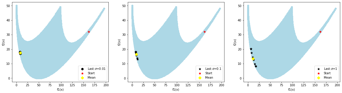
5.2 Test problems with added noise
Test 1. Firstly, we go over a function with a convex Pareto front, [28]. Let the problem be defined as follows:
| (51) |
where,
To achieve randomness and emulate our assumptions, we add the noise to function and gradient values in the following way:
where , , Noises are scaled respectively with the trust region radius , which emulates the probabilistic full linearity in a way. We posed 3 different scenarios, in which we changed the variance of the noise. Each of the runs had 10 independent simulations, with fixed 500 iterations.
The following figures show how modifying the variance of the noise ’increases’ randomness, and changes the location of the last iteration, however it doesn’t change the fact that the algorithm finds a Pareto critical point. By increasing the variance of the noise, we can notice that last iterations of simulations disperse throughout the set of Pareto criticality, which for this problem is on the Pareto front.
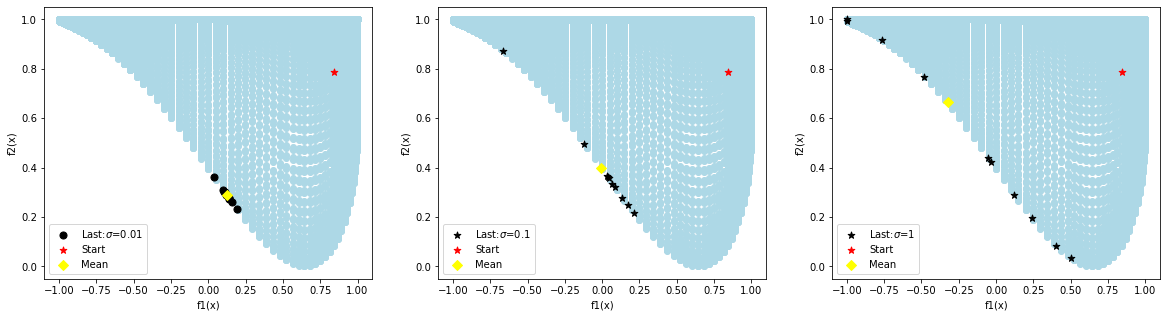
Test 2. The second example involves two functions, which together generate a non convex front, [28]. We are solving:
| (52) |
where,
As in the first example the noise is generated in the following way:
where , Three separate experiments have been conducted, with 10 simulations each and 500 iterations. It can be seen that even though the standard deviation increases the SMOP algorithm successfully identifies a Pareto critical point for problems with both convex and non convex front.
5.3 Machine learning (logistic regression)
When handling sensitive data in machine learning, there is a significant risk of developing models that exhibit discriminatory behavior. Unfairness emerges when the performance of a model measured in terms of accuracy or another metric, varies across subgroups of data that are categorized based on sensitive attributes, such as race, gender or age [21]. For more on this topic, see [2],[18], [31],[32],[33]. Such differences can have real-world consequences, particularly in applications where the subgroups represent actual individuals, such as in hiring systems, healthcare diagnostics, or judicial decision-making. These biases can create systemic inequalities and harm marginalized communities.
Achieving fairness in machine learning involves ensuring that the predictive performance of a model is consistent across different subgroups. Hence, fairness can be defined as the condition where no subgroup experiences significantly worse outcomes. To address this issue, one effective approach is to formulate the scalar optimization problem as a multi-objective one. By splitting the data based on the sensitive attributes and treating the performance on each subgroup as a separate objective, it is possible to train models that find more balanced optimum values.
The problem we consider is optimization of a regularized logistic regression loss function, as in [21]:
| (53) |
where represents model coefficients we are trying to find, coefficient vector without the intercept, the feature vector of sample, its respective label and the training set size.
In order to create a multi-objective problem, we choose a feature, split the data with respect to it, and create a function for each subgroup. For the sake of simplicity, for each dataset, two subgroups were made. The loss functions for such problem are:
where is the size of the sample subgroup, and hence the problem becomes:
| (54) |
The approximation of function and gradient values is done by an adaptive subsampling strategy , motivated by the result from [25] (Lemma 4). Namely, for each subgroup we get provided that
| (55) |
where is the upper bound of . Although this kind of bound is not easy to obtain in general, for logistic regression problems it is possible to use e.g.
Similar bound can be derived for the gradients where we get provided that
| (56) |
with
In our tests, we use only estimated bounds where the upper-bounds are replaced by some constants and the sample size behaves like
Approximate functions are created in the following way:
Gradients of the approximate functions can then be used to approximate gradients of the true functions, i.e. , hence Assumption 3 is satisfied. The probabilities should theoretically converge to 1, however choosing in our implementations demonstrated strong performance. This way, the probability that both function approximations and are -close to and respectively is greater than . Using these functions we create probabilistically FL models with high enough probability. This has theoretical implications, as seen in the proof of Theorem (4).
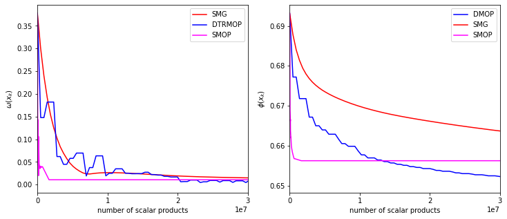
We compared the SMOP algorithm with the deterministic trust region [30] (DMOP), and the stochastic multi-gradient [21] (SMG). The evaluation focuses on the algorithms’ performance by measuring the value of true marginal function , and scalar representation in terms of number of scalar products at each iteration. It is important to notice that for each function evaluation of , we have scalar products. In this manner, we demonstrate how the SMOP algorithm achieves significant improvements in performance while utilizing only a fraction of the available data. This highlights the algorithms effectiveness in leveraging limited resources, making it particularly valuable in scenarios where data collection is expensive.
The comparison for covtype [7] dataset is shown, which has 450000 training size, and attribute dimension 54. The data is split in a way that and . Due to the stochasticity of the algorithms and the nature of the multiobjective problem, the resulting Pareto critical points can be different. This implies that the values of will not necessarily be the same for different algorithms, or even for subsequent simulations of the same algorithm. However, the fact that converges to zero shows that the algorithms finds a critical value. The efficiency of the algorithm is emphasized when considering the number of scalar products necessary to reach the near-optimality threshold, as seen in Figure3. Notice how the resulting values are different for each algorithm.
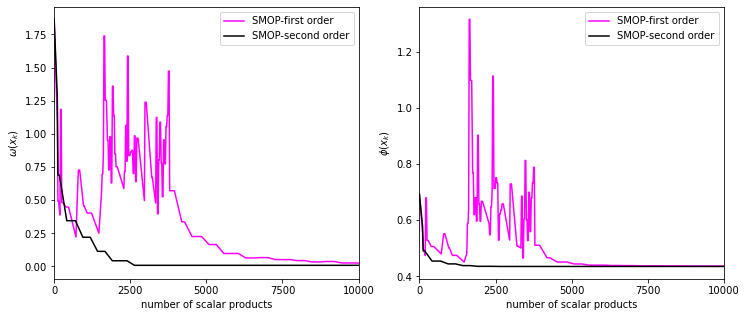
5.4 First vs second order algorithm
Although the models are designed to have Hessian values, in the previous applications we used only the first order information, i.e. . The algorithm uses models to calculate the trust region ratio, hence the quadratic model should more precisely determine whether the step is accepted, and whether the radius should be increased or decreased. Using the second order information, we expect our algorithm to be more precise and stable in the long run. We compare the first and the second order versions of SMOP, using the heart dataset [19]. The heart dataset has 242 samples, and the attribute dimension is 14. In a similar way, by splitting the data into two sets , we convert the optimization problem (53) into a multi-objective one (54). We approximate the Hessian with the subsampled Hessians using the same subsample as for the functions approximations (55). The following Figure 4 shows the convergence to a critical point of both versions, and ilustrates the comparative advantage of the second order method.
5.5 Finding Pareto front
As previously mentioned, the goal of the SMOP algorithm is to identify a Pareto critical point. However, in some cases, we may wish to better understand the structure of the entire Pareto front, or even find a specific optimal point within it. Hence, approximating the Pareto front is an important feature to implement. Using the standard front finding technique, from [14], we successfully find the Pareto front for different problems. The notion of this Pareto finding method is to approximate the Pareto front using a set of random points. At each iteration this approximation set is expanded by generating perturbed points around the existing elements in the set. Predetermined number of SMOP iterations is then applied to the existing points, after which the results are also added to the approximation set. To refine the approximation, all dominated points are removed from the set, leaving only the non dominated points to serve as the updated Pareto approximation for the next iteration. Point is said to be dominated if there exists , such that , i.e. for . The procedure is described in the following way:
Algorithm 2.(Pareto front SMOP)
-
Step 0. Generate intial Pareto front Select parameters .
-
Step 1. Set . For each point in , add points to from the neighborhood of .
-
Step 2. For each point in , repeat times: Apply iterations of SMOP with as a starting point. Add the final iteration to
-
Step 3. Remove all dominated points from . Go to Step 1.
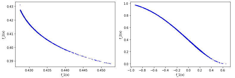
The procedure was implemented for convex and nonconvex case. The following figures show the Pareto front for Logistic regression example (54) on heart dataset [19] and for Test problem 2 (52). By choosing different it is possible to get a sparser front with less details, hence depending on the problem, the cost of finding the front can be reduced at the expense of Pareto front information.
5.6 Conclusion
We have proposed a multi-objective trust region method which utilizes approximate functions, gradients and Hessians. The method is designed to operate under the key assumptions that the approximation accuracy of models is achieved with high enough probability and that the approximate gradients are close enough to the gradients of the approximate functions. The theoretical contribution of this work is the proof of almost sure convergence to a Pareto critical point. We presented several numerical experiments that showcase the algorithm’s efficient practical performance. We highlighted its capability to effectively solve multi-objective optimization problems while maintaining low computational cost. Additionally, we implemented a Pareto finding routine in order to find the Pareto front. Future work could include the generalization of fully quadratic models or techniques such as additional sampling.
Acknowledgments
This work was supported by the Science Fund of the Republic of Serbia, Grant no. 7359, Project LASCADO.
References
- [1] Bandeira, A.S., Scheinberg, K. Vicente, L.N. (2014) Convergence of trust-region methods based on probabilistic models, SIAM Journal on Optimization, 24(3), 1238-1264.
- [2] Barocas, S., Hardt, M. Narayanan, A. (2017) Fairness in machine learning. NIPS Tutorial, 1.
- [3] Bellavia, S., Krejić, N. Morini, B. (2020) Inexact restoration with subsampled trust-region methods for finite-sum minimization. Comput Optim Appl 76, 701–736.
- [4] Berkemeier, M. Peitz, S. (2021) Derivative-Free Multiobjective Trust Region Descent Method Using Radial Basis Function Surrogate Models, Math. Comput. Appl., 26, 31.
- [5] Berahas A. S., Bollapragada R. Nocedal J. (2020) An Investigation of Newton-Sketch and Subsampled Newton Methods, Optimization Methods and Software, 35(4), 661–680.
- [6] Blanchet, J., Cartis, C., Menickelly, M. Scheinberg, K. (2019) Convergence Rate Analysis of a Stochastic Trust-Region Method via Supermartingales, INFORMS Journal on Optimization, 1(2), 92-119.
- [7] Blackard, J. (1998) Covertype [Dataset]. UCI Machine Learning Repository.
- [8] Bollapragada, R., Byrd, R. Nocedal, J. (2019) Exact and Inexact Subsampled Newton Methods for Optimization, IMA Journal of Numerical Analysis, 39(20), 545-578.
- [9] Bottou, L., Curtis F.E., Nocedal, J. (2018) Optimization Methods for LargeScale Machine Learning, SIAM Review, 60(2), 223-311.
- [10] Byrd, R.H., Hansen, S.L., Nocedal, J. Singer, Y. (2016) A Stochastic QuasiNewton Method for Large-Scale Optimization, SIAM Journal on Optimization, 26(2), 1008-1021
- [11] Byrd, R.H., Chin, G.M., Nocedal, J. Wu, Y. (2012) Sample size selection in optimization methods for machine learning, Mathematical Programming, 134(1), 127-155.
- [12] Chen, R., Menickelly, M. Scheinberg, K. (2018) Stochastic optimization using a trust-region method and random models, Math. Program., 169, 447–487.
- [13] Curtis, F.E., Scheinberg, K. Shi R. (2018) A Stochastic Trust Region Algorithm Based on Careful Step Normalization, INFORMS Journal on Optimization, 1(3), 200-220.
- [14] Custodio, A.L., Madeira, J.A., Vaz, A.I.F. Vicente, L. N. (2011) Direct multisearch for multiobjective optimization. SIAM J. Optim, 21, 1109-1140.
- [15] Durrett, R. (2010) Probability: Theory and Examples. Cambridge Series in Statistical and Probabilistic Mathemat- ics. Cambridge University Press, Cambridge, fourth edition.
- [16] Fliege, J. Svaiter, B.F. (2000) Steepest Descent Methods for Multicriteria Optimization, Mathematical Methods of Operations Research, 51, 479-494.
- [17] Fukuda, E. H. Drummond, L. M. G. (2014) A survey on multiobjective descent methods. Pesq. Oper. 34 (3).
- [18] Hardt, M., Price, E. Srebro, N. (2016) Equality of opportunity in supervised learning. Advances in neural information processing systems, 3315-3323.
- [19] Janosi, A., Steinbrunn, W., Pfisterer, M. Detrano, R. (1989) Heart Disease [Dataset]. UCI Machine Learning Repository.
- [20] Krejić, N., Krklec Jerinkić, N., Martínez, A. Yousefi, M. (2024) A non-monotone trust-region method with noisy oracles and additional sampling. Comput Optim Appl 89, 247–278.
- [21] Liu, S. Vicente, L.N. (2024) The stochastic multi-gradient algorithm for multi-objective optimization and its application to supervised machine learning, Ann Oper Res, 339, 1119–1148.
- [22] Robbins, H. Monro, S. (2011) A Stochastic Approximation Method SIAM J. Optim, 21, 1109-1140.
- [23] Sawaragi, Y., Nakayama, H. Tanino, T. (1985) Theory of multiobjective optimization, Elsevier, MR 807529
- [24] Robbins, H. Siegmund, D. (1971) A convergence theorem for non negative almost supermartingales and some applications, Optimizing Methods in Statistics, 233-257.
- [25] Roosta-Khorasani, F. Mahoney, M. W. (2016) Sub-Sampled Newton Methods I: Globally Convergent Algorithms, arXiv:1601.04737
- [26] Tanabe, H., Fukuda, E.H. Yamashita, N.(2019) Proximal gradient methods for multiobjective optimization and their applications Comput. Optim. Appl. 72, 339–361.
- [27] Thomann, J. Eichfelder, G. (2019) A Trust-Region Algorithm for Heterogeneous Multiobjective Optimization, SIAM Journal on Optimization, 29, 1017 - 1047.
- [28] Thomann, J. Eichfelder, G. (2019) Numerical results for the multiobjective trust region algorithm MHT, Data in Brief, 25.
- [29] Tripuraneni, N., Stern, M., Jin, C., Regier, J. Jordan, M.I. (2018) Stochastic Cubic Regularization for Fast Nonconvex Optimization Advances in Neural Information Processing Systems 31.
- [30] Villacorta, K.D.V., Oliveira, P.R. Soubeyran, A, (2014) A Trust-Region Method for Unconstrained Multiobjective Problems with Applications in Satisficing Processes, J Optim Theory Appl 160, 865–889.
- [31] Woodworth, B., Gunasekar, S., Ohannessian, M.I. Srebro, N. (2017) Learning non-discriminatory predictors. Conference on Learning Theory, 1920-1953.
- [32] Zafar, M.B., Valera, I., Gomez Rodriguez, M. Gummadi, K.P. (2017) Fairness constraints: Mechanisms for fair classiffication. Artifficial Intelligence and Statistics, 962-970.
- [33] Zemel, R., Wu, Y., Swersky, K., Pitassi, T. Dwork, C. (2013) Learning fair representations. International Conference on Machine Learning, 325-333.