Simple proof of robustness for Bayesian heavy-tailed linear regression models

Abstract

In the Bayesian literature, a line of research called resolution of conflict is about the characterization of robustness against outliers of statistical models. The robustness characterization of a model is achieved by establishing the limiting behaviour of the posterior distribution under an asymptotic framework in which the outliers move away from the bulk of the data. The proofs of the robustness characterization results, especially the recent ones for regression models, are technical and not intuitive, limiting the accessibility and preventing the development of theory in that line of research. We highlight that the proof complexity is due to the generality of the assumptions on the prior distribution. To address the issue of accessibility, we present a significantly simpler proof for a linear regression model with a specific prior distribution corresponding to the one typically used. The proof is intuitive and uses classical results of probability theory. To promote the development of theory in resolution of conflict, we highlight which steps are only valid for linear regression and which ones are valid in greater generality. The generality of the assumption on the error distribution is also appealing; essentially, it can be any distribution with regularly varying or log-regularly varying tails. So far, there does not exist a result in such generality for models with regularly varying distributions. Finally, we analyse the necessity of the assumptions.

¹Department of Mathematics and Statistics, Université de Montréal.

Keywords: log-regularly varying functions, outliers, Student’s $t$ distribution, regularly varying functions.

1 Introduction

The topic of robustness against outliers is classical in statistics. An objective when studying this topic is to evaluate whether commonly used statistical methods are robust against outliers or not. A method is deemed not robust if a single observation can have an arbitrary impact on the estimation. A canonical example of a non-robust method is a linear regression with normal errors, as seen in Figure 1. In this figure, we present the result of a simple numerical experiment based on $n=20$ observations $y_{1},\ldots,y_{n}$ of a dependent variable and $n$ data points $(x_{1},x_{2},\ldots,x_{n})=(1,2,\ldots,n)$ of an explanatory variable. The observations $y_{1},\ldots,y_{n}$ were first sampled using a linear regression model with an intercept and slope coefficients both equal to 1 and independent errors each having a standard normal distribution. The observation $y_{n}$ was then gradually increased to obtain a sequence of data sets. For each data set, the slope coefficient is estimated using the posterior mean in a Bayesian analysis; see Appendix A for the details. In Figure 1, we also present estimation results for the Bayesian Student’s $t$ linear regression which is the preferred Bayesian robust alternative. The code to reproduce our numerical results is available online (see ancillary files on the arXiv page of the paper).

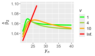
Figure 1: Posterior mean of the slope coefficient $\beta_{2}$ as $y_{n}$ increases for the Student’s $t$ linear regression with different degrees of freedom $\nu$, where “Inf.” represents the normal linear regression.

The frequentist literature on the topic of robustness against outliers is rich, especially in linear regression, with celebrated work like that of Huber (1973) and Beaton and Tukey (1974) about the Huber and Tukey’s biweight M-estimators. The Bayesian literature is more sparse. A line of research in the Bayesian literature, called resolution of conflict (O’Hagan and Pericchi, 2012), aims to (mathematically) characterize the limiting behaviour of robust alternatives as outliers move further and further away from the bulk of the data, like the limiting behaviour observed in Figure 1 for the Student’s $t$ linear regression. The characterization is achieved by studying the limit of the associated posterior densities. Studying the limit of a posterior density is not easy due essentially to the presence of an integral in the denominator representing the marginal density evaluated at the observations or, equivalently, the normalizing constant.

First works in resolution of conflict focused on the location model (e.g., Dawid (1973), O’Hagan (1979) and Desgagné and Angers (2007)) and the location–scale model (e.g., Andrade and O’Hagan (2011) and Desgagné (2015)). In recent years, the focus has been on linear regression (Desgagné and Gagnon, 2019; Gagnon et al., 2020, 2021; Gagnon, 2023; Gagnon and Hayashi, 2023; Hamura et al., 2022, 2024; Hamura, 2024), generalized linear models (Gagnon and Wang, 2024; Hamura et al., 2025) and multivariate modelling (Andrade, 2023). The proofs of the robustness characterization results are generally highly technical and not intuitive, limiting the accessibility and preventing the development of theory in that line of research. For instance, the first proof for the usual linear regression model, in Gagnon et al. (2020), involves the decomposition of the parameter space in mutually exclusive sets for which it is difficult to develop an intuition and which makes the majority of the steps in the proof technical, in addition to making the proof lengthy.

Hamura (2024) recently highlighted the issue of accessibility. With the goal of improving accessibility of robustness characterization results and their proofs, the author presented a proof for a linear regression with a specific heavy-tailed error distribution. We however consider the attempt unsatisfactory as the heavy-tailed distribution assumed is not used in practice and, perhaps more importantly, the proof technique is the same as in Gagnon et al. (2020) with the decomposition of the parameter space into mutually exclusive sets; the proof is thus not intuitive and highly technical. The goal with the current paper is to address the issue of accessibility in a way that is, in our opinion, more effective.

The approach is different than in Hamura (2024): we consider a specific prior distribution instead, this prior distribution being the one typically used in Bayesian normal linear regression given its conjugacy properties. The prior distribution is a conditional normal distribution for the regression coefficients and an inverse-gamma distribution for the squared scale of the errors. The framework can thus be seen as that where a statistician is usually happy with the Bayesian normal linear regression (with this prior distribution), but this statistician worries that it may not be adapted for the current data set for which the presence of outliers is probable; thus the statistician wants to gain robustness and (only) changes the distribution assumption on the errors. By considering this specific prior distribution, we are able to present a robustness characterization result with a significantly simpler proof, to the extent that we are able to consider a remarkably general distribution assumption on the errors while keeping the proof simple; essentially, it can be any distribution with regularly varying or log-regularly varying tails. The proof is intuitive, uses classical probability arguments and is significantly shorter. In the proof, we highlight which steps are only valid for linear regression and which ones are valid in greater generality, aiming to promote the development of theory in resolution of conflict.

We now present how the rest of the paper is organized. In Section 2, we present in more detail the context, the model and the assumptions. In Section 3, we present the robustness characterization result and, in Section 4, its proof.

We finish this section with a general remark about robustness: there is of course a price to pay for a gain in robustness like that observed in Figure 1 for the Student’s $t$ linear regression. The price is twofold. Firstly, there is a loss in efficiency, in the sense that, in the absence of outliers, the estimation is less efficient than with the benchmark (e.g., normal linear regression). The efficiency loss has been precisely measured for the Student’s $t$ model in linear regression in Gagnon and Hayashi (2023). Secondly, there is an added computational complexity as all integrals need to be approximated using numerical methods, typically Markov chain Monte Carlo methods, even for linear regression. Hamiltonian Monte Carlo (Duane et al., 1987; Neal, 2011) has been used to approximate the posterior means in Figure 1; see Appendix A for more details. Variable selection can be performed using a reversible jump algorithm (Green, 1995, 2003). Efficient informed and non-reversible variants have been proposed in Gagnon (2021) and Gagnon and Maire (2024), respectively.

2 Context, model and assumptions

Let us assume that we have access to a data set of the form $\{\mathbf{x}_{i},y_{i}\}_{i=1}^{n}$, where $\mathbf{x}_{1},\ldots,\mathbf{x}_{n}\in\operatorname{\mathbb{R}}^{p}$ are $n\in\operatorname{\mathbb{N}}$ vectors of explanatory variable data points and $y_{1},\ldots,y_{n}\in\operatorname{\mathbb{R}}$ are $n$ observations of a dependent variable, $p$ being a positive integer. Let us assume that one is interested in modelling the dependent variable through its relationship with the explanatory variables and, more specifically, in using a linear regression model. In such a model, it is assumed that $y_{1},\ldots,y_{n}$ are realizations of $n$ random variables $Y_{1},\ldots,Y_{n}$ defined as follows:

$$Y_{i}=\mathbf{x}_{i}^{T}\bm{\beta}+\sigma\varepsilon_{i},\quad i=1,\ldots,n,$$ (1)

where $\bm{\beta}=(\beta_{1},\ldots,\beta_{p})^{T}\in\operatorname{\mathbb{R}}^{p}$ is a vector of regression coefficients, $\sigma>0$ is a scale parameter and $\varepsilon_{1},\ldots,\varepsilon_{n}\in\operatorname{\mathbb{R}}$ are standardized errors. In an homoscedastic model, it is assumed that $\varepsilon_{1},\ldots,\varepsilon_{n}$ are independent and identically distributed random variables, each having a probability density function (PDF) denoted here by $f$. In a Bayesian model, it is typically assumed that the two groups of random variables $(\varepsilon_{1},\ldots,\varepsilon_{n})$ and $(\bm{\beta},\sigma)$ are independent. Also, the vectors $\mathbf{x}_{1},\ldots,\mathbf{x}_{n}$ are typically considered to be fixed and known, that is not realizations of random variables, contrarily to $y_{1},\ldots,y_{n}$.

We now present the assumptions on $f$.

Assumption 1.

The PDF $f$ is strictly positive, symmetric and monotonic, that is $f(y)>0$ and $f(y)=f(|y|)$ for all $y$, and, for any $|y_{2}|\geq|y_{1}|$, $f(|y_{2}|)\leq f(|y_{1}|)$. Also, it is bounded, that is there exists a constant $C>0$ such that $f\leq C$. Finally, either of the following holds:

1. regularly varying function: there exist constants $C_{f}>0$ and $\alpha>0$ such that

   $$\lim_{y\rightarrow\pm\infty}\frac{f(y)}{C_{f}\,|y|^{-(\alpha+1)}}=1;$$

2. log-regularly varying function: there exist constants $C_{f}>0$ and $\alpha>0$ such that

   $$\lim_{y\rightarrow\pm\infty}\frac{f(y)}{C_{f}\,|y|^{-1}(\log|y|)^{-(\alpha+1)}}=1.$$

The first part of Assumption 1 (positivity, symmetry, monotonicity and boundedness) represents regularity conditions which simplify the theoretical analysis. The second part is about tail thickness, heavy tails being essentially necessary for robustness. In this second part, we assume that $f$ is either regularly varying or log-regularly varying. Regularly varying functions are well known (see, e.g., Resnick (2007) for a reference) and appear in many contexts, such as statistical network modelling (Caron and Fox, 2017) and, of course, robustness against outliers as in the current paper. Note that we made an abuse of terminology in Assumption 1 as the definition of regularly varying function is slightly more general; we presented this version to simplify. We will nevertheless use the terminology “regularly varying functions” to refer to functions satisfying (i) in Assumption 1. As stated in Proposition 1, the preferred PDF in robustness, the Student’s $t$, satisfies Assumption 1 as a regularly varying function.

Proposition 1.

Let $f$ be a Student’s $t$ PDF with $\nu>0$ degrees of freedom, that is

$$f(y)=\frac{\Gamma\left(\frac{\nu+1}{2}\right)}{\sqrt{\pi\nu}\,\Gamma\left(\frac{\nu}{2}\right)}\left(1+\frac{y^{2}}{\nu}\right)^{-\frac{\nu+1}{2}},\quad y\in\operatorname{\mathbb{R}},$$

where $\Gamma$ is the gamma function. Then, Assumption 1 is satisfied.

Proof of Proposition 1.

It is straightforward to verify the first part of Assumption 1. It can be readily verified that $f$ is regularly varying using

$$C_{f}=\frac{\Gamma\left(\frac{\nu+1}{2}\right)\nu^{\nu/2}}{\sqrt{\pi}\,\Gamma\left(\frac{\nu}{2}\right)}$$

and $\alpha=\nu$. ∎

The notion of log-regularly varying functions appeared more recently in Desgagné (2015) in the context of robustness against outliers to achieve what is referred to as whole robustness for the location–scale model (we will return to the concept of whole robustness in Section 3). As for regularly varying functions, we made an abuse of terminology in Assumption 1 as the definition of log-regularly varying function is slightly more general. We will carry on with this abuse of terminology. An example of log-regularly varying PDFs is the log-Pareto-tailed normal (LPTN). The central part of this continuous PDF coincides with the standard normal and the tails are log-Pareto, hence its name. It has an hyperparameter $\rho\in(2\Phi(1)-1,1)\approx(0.6827,1)$ and is given by

$$f(y)=\left\{\begin{array}[]{lcc}\varphi(y)&\text{ if }&|y|\leq\vartheta,\cr\varphi(\vartheta)\,\frac{\vartheta}{|y|}\left(\frac{\log\vartheta}{\log|y|}\right)^{\lambda+1}&\text{ if }&|y|>\vartheta,\cr\end{array}\right.$$

where $\vartheta>1$ and $\lambda>0$ are functions of $\rho$ with

$$\vartheta=\Phi^{-1}((1+\rho)/2)=\{\vartheta:\mathbb{P}(-\vartheta\leq Z\leq\vartheta)=\rho\,\text{ for }\,Z\,\sim\,\mathcal{N}(0,1)\},$$

$$\lambda=2(1-\rho)^{-1}\varphi(\vartheta)\,\vartheta\log(\vartheta),$$

$\varphi$ and $\Phi$ being the PDF and cumulative distribution function of a standard normal distribution, respectively.

Proposition 2.

Let $f$ be a LPTN PDF with $\rho\in(2\Phi(1)-1,1)$. Then, Assumption 1 is satisfied.

Proof of Proposition 2.

It is straightforward to verify the first part of Assumption 1. It can be readily verified that $f$ is log-regularly varying using

$$C_{f}=\varphi(\vartheta)\,\vartheta\,(\log\vartheta)^{\lambda+1}$$

and $\alpha=\lambda$. ∎

We now present the assumptions on the prior distribution.

Assumption 2.

The prior distribution is such that: $\bm{\beta}$ given $\sigma$ has a normal distribution with a mean of $\mathbf{0}$ and a covariance matrix of $\sigma^{2}\mathbf{I}_{p}$, where $\mathbf{I}_{p}$ is the identity matrix of size $p$, and $\sigma^{2}$ has an inverse-gamma distribution with any shape and scale parameters.

As mentioned in Section 1, this prior distribution is commonly used in Bayesian linear regression (see, e.g., Raftery et al. (1997)). With a (conditional) normal distribution on $\bm{\beta}$, one has to be careful with the potential conflict between the prior information and that carried by the data (Gagnon, 2023). Note that this is true also for $\sigma$ given that the inverse-gamma PDF has a thin left tail. Ideally, the scale parameter of the inverse-gamma would be of the same order of magnitude as $\sigma^{2}$ to mitigate the effect of conflicting prior information. A small value for the shape parameter makes the inverse-gamma PDF relatively flat and thus yields a prior distribution that is as weakly informative as possible for this type of prior distributions.

3 Robustness characterization result

To characterize the robustness of the model in (1) (depending on $f$), we study it under an asymptotic framework where the outliers move further and further away from the bulk of the data. We mathematically represent this asymptotic framework by considering that the outliers move along particular paths (as in, e.g., Gagnon et al. (2020) and Hamura et al. (2022)). The mathematical representation allows for a general definition of outliers, that is couples $(\mathbf{x}_{i},y_{i})$ whose components are incompatible with the trend in the bulk of the data. Let us consider for example that there is an element in $\mathbf{x}_{i}$ that makes the combination of $\mathbf{x}_{i}$ with $y_{i}$ incompatible. Equivalently, in this example, we can consider that, compared with the trend in the bulk of the data, the value of $y_{i}$ is either too small or too large for this $\mathbf{x}_{i}$ . We can thus allow for this general definition of outliers by considering an asymptotic framework where the vectors $\mathbf{x}_{i}$ are fixed (but potentially extreme) and the observations $y_{i}$ are such that

$$|y_{i}|=a_{i}+b_{i}\omega,\quad i=1,\ldots,n,$$

where $a_{i}>0$ is a constant, $b_{i}=0$ if the data point is a non-outlier and $b_{i}\geq 1$ if it is an outlier, and then we let $\omega\rightarrow\infty$.

Under such an asymptotic framework, we obtain a sequence of posterior distributions, indexed by $\omega$, and we want to understand what a posterior distribution in this sequence looks like when $\omega$ is large. We will prove theoretical asymptotic results characterizing the limiting posterior distribution which imply that, for the outlying data points with $\mathbf{x}_{i}$ fixed (but potentially extreme), there exist large enough values for $|y_{i}|=a_{i}+b_{i}\omega$ such that the associated posterior distribution is similar to the limiting one. The location of the point $(\mathbf{x}_{i},y_{i})$ has an impact on how large $|y_{i}|$ needs to be; for instance, it needs be larger when $\mathbf{x}_{i}$ is extreme, justifying the use of different $a_{i}$ and $b_{i}$ for the different points. For a real data set with (fixed) outliers, the goal of this representation is to be able to choose values for all $a_{i}$ and $b_{i}$ and a value for $\omega$ so that this data set is obtained.

We now present definitions that will allow to state the robustness characterization result. Let us define the index set of outlying data points by: $\mathrm{O}:=\{i:b_{i}\geq 1\}$. The index set of non-outlying data points is thus given by: $\mathrm{O}^{\mathsf{c}}:=\{1,\ldots,n\}\setminus\mathrm{O}$. We also define the set of non-outlying observations: $\mathbf{y}_{\mathrm{O}^{\mathsf{c}}}:=\{y_{i}:i\in\mathrm{O}^{\mathsf{c}}\}$. Let us denote by $\pi$ the prior distribution of $(\bm{\beta},\sigma)$. We consider that it is not in conflict with trend in the bulk of the data to focus on robustness against outliers; see Gagnon (2023) for a study of robustness of heavy-tailed prior distributions against conflicting prior information in regression. Let us denote by $\pi_{\omega}(\,\cdot\,,\cdot\mid\mathbf{y})$ a posterior distribution in the sequence indexed by $\omega$, with a posterior density, denoted by $\pi_{\omega}(\,\cdot\,,\cdot\mid\mathbf{y})$ as well to simplify, which is such that

$$\pi_{\omega}(\bm{\beta},\sigma\mid\mathbf{y})=\pi(\bm{\beta},\sigma)\left[\prod_{i=1}^{n}(1/\sigma)f((y_{i}-\mathbf{x}_{i}^{T}\bm{\beta})/\sigma)\right]\Bigg{/}m_{\omega}(\mathbf{y}),\quad\bm{\beta}\in\operatorname{\mathbb{R}}^{p},\sigma>0,$$ (2)

where $\mathbf{y}=(y_{1},\ldots,y_{n})^{T}$ and

$$m_{\omega}(\mathbf{y})=\int_{\operatorname{\mathbb{R}}^{p}}\int_{0}^{\infty}\pi(\bm{\beta},\sigma)\left[\prod_{i=1}^{n}(1/\sigma)f((y_{i}-\mathbf{x}_{i}^{T}\bm{\beta})/\sigma)\right]\,\mathrm{d}\sigma\,\mathrm{d}\bm{\beta},$$

if $m_{\omega}(\mathbf{y})<\infty$, a situation where the posterior distribution is proper and thus well defined.

From (2), we understand that the limiting behaviour of the (conditional) PDF of $Y_{i}$ evaluated at an outlying point is central to the characterization of the robustness properties of a robust alternative. We now present a proposition about this limiting behaviour.

Proposition 3.

Suppose that Assumption 1 holds. For all $\bm{\beta}\in\operatorname{\mathbb{R}}^{p}$ and $\sigma>0$,

$$\lim_{y_{i}\rightarrow\pm\infty}\frac{(1/\sigma)f((y_{i}-\mathbf{x}_{i}^{T}\bm{\beta})/\sigma)}{g(\sigma)f(y_{i})}=1,$$

where $g(\sigma)=\sigma^{\alpha}$ if $f$ is a regularly varying function or $g(\sigma)=1$ if $f$ is a log-regularly varying function.

Proof of Proposition 3.

Let us first consider the case where $f$ is regularly varying. For all $\bm{\beta}\in\operatorname{\mathbb{R}}^{p}$ and $\sigma>0$,

$$\lim_{y_{i}\rightarrow\pm\infty}\frac{(1/\sigma)f((y_{i}-\mathbf{x}_{i}^{T}\bm{\beta})/\sigma)}{f(y_{i})}$$

$$\quad=\lim_{y_{i}\rightarrow\pm\infty}\frac{f((y_{i}-\mathbf{x}_{i}^{T}\bm{\beta})/\sigma)}{C_{f}\,|(y_{i}-\mathbf{x}_{i}^{T}\bm{\beta})/\sigma|^{-(\alpha+1)}}\frac{C_{f}\,|y_{i}|^{-(\alpha+1)}}{f(y_{i})}\frac{(1/\sigma)C_{f}\,|(y_{i}-\mathbf{x}_{i}^{T}\bm{\beta})/\sigma|^{-(\alpha+1)}}{C_{f}\,|y_{i}|^{-(\alpha+1)}}=\sigma^{\alpha}.$$

Let us now consider the case where $f$ is log-regularly varying. For all $\bm{\beta}\in\operatorname{\mathbb{R}}^{p}$ and $\sigma>0$,

$$\lim_{y_{i}\rightarrow\pm\infty}\frac{(1/\sigma)f((y_{i}-\mathbf{x}_{i}^{T}\bm{\beta})/\sigma)}{f(y_{i})}$$

$$\quad=\lim_{y_{i}\rightarrow\pm\infty}\frac{f((y_{i}-\mathbf{x}_{i}^{T}\bm{\beta})/\sigma)}{C_{f}\,|(y_{i}-\mathbf{x}_{i}^{T}\bm{\beta})/\sigma|^{-1}(\log|(y_{i}-\mathbf{x}_{i}^{T}\bm{\beta})/\sigma|)^{-(\alpha+1)}}\frac{C_{f}\,|y_{i}|^{-1}(\log|y_{i}|)^{-(\alpha+1)}}{f(y_{i})}$$

$$\hskip 227.62204pt\times\frac{C_{f}\,|y_{i}-\mathbf{x}_{i}^{T}\bm{\beta}|^{-1}(\log|(y_{i}-\mathbf{x}_{i}^{T}\bm{\beta})/\sigma|)^{-(\alpha+1)}}{C_{f}\,|y_{i}|^{-1}(\log|y_{i}|)^{-(\alpha+1)}}=1.$$

∎

Under Assumption 1, we thus expect the PDF term of each outlier in (2) to behave like $g(\sigma)f(y_{i})\propto g(\sigma)$ asymptotically. The results that we present below are specifically about this. We prove convergence of the posterior distribution towards $\pi(\,\cdot\,,\cdot\mid\mathbf{y}_{\mathrm{O}^{\mathsf{c}}})$ which is such that

$$\pi(\bm{\beta},\sigma\mid\mathbf{y}_{\mathrm{O}^{\mathsf{c}}})=\pi(\bm{\beta},\sigma)\,g(\sigma)^{|\mathrm{O}|}\left[\prod_{i\in\mathrm{O}^{\mathsf{c}}}(1/\sigma)f((y_{i}-\mathbf{x}_{i}^{T}\bm{\beta})/\sigma)\right]\Bigg{/}m(\mathbf{y}_{\mathrm{O}^{\mathsf{c}}}),\quad\bm{\beta}\in\operatorname{\mathbb{R}}^{p},\sigma>0,$$

where $|\mathrm{O}|$ is the cardinality of the set $\mathrm{O}$, that is the number of outliers, and

$$m(\mathbf{y}_{\mathrm{O}^{\mathsf{c}}})=\int_{\operatorname{\mathbb{R}}^{p}}\int_{0}^{\infty}\pi(\bm{\beta},\sigma)\,g(\sigma)^{|\mathrm{O}|}\left[\prod_{i\in\mathrm{O}^{\mathsf{c}}}(1/\sigma)f((y_{i}-\mathbf{x}_{i}^{T}\bm{\beta})/\sigma)\right]\,\mathrm{d}\sigma\,\mathrm{d}\bm{\beta},$$

if $m(\mathbf{y}_{\mathrm{O}^{\mathsf{c}}})<\infty$, a situation where the limiting posterior distribution is proper and thus well defined. Note that we abused notation by writing, for instance, $\pi(\,\cdot\,,\cdot\mid\mathbf{y}_{\mathrm{O}^{\mathsf{c}}})$ as the latter is not the conditional distribution given only the non-outliers in the case where $f$ is regularly varying; there is an additional term, $g(\sigma)^{|\mathrm{O}|}=\sigma^{|\mathrm{O}|\alpha}$, in the definitions above.

When $f$ is log-regularly varying, there is asymptotically no trace of the outliers in the posterior distribution as $g(\sigma)=1$. The robust alternative thus acts automatically like practitioners would and excludes the outliers when they are far enough from the bulk of the data and there is no doubt as to whether they really are outliers. Such a robust alternative is said to achieve whole robustness. When $f$ is regularly varying, there is asymptotically a trace of the outliers in the posterior distribution, namely $g(\sigma)=\sigma^{\alpha}$ for each outlier. It is nevertheless possible to obtain a limit which, by definition, does not depend on $\omega$, the latter representing in a sense the source of outlyingness. Such a robust alternative is thus said to achieve partial robustness. Note that, typically, the impact of observations gradually diminish when they are artificially moved away from the bulk of the data, as observed in Figure 1. Moderately far observations thus have a certain influence, reflecting uncertainty about the nature of these observations in a grey zone (outliers versus non-outliers).

In order to state the robustness characterization result, we need a guarantee that all posterior distributions are well defined ($\pi_{\omega}(\,\cdot\,,\cdot\mid\mathbf{y})$ and $\pi(\,\cdot\,,\cdot\mid\mathbf{y}_{\mathrm{O}^{\mathsf{c}}})$). We present an assumption on the number of outliers $|\mathrm{O}|$, or equivalently the number of non-outliers $|\mathrm{O}^{\mathsf{c}}|=n-|\mathrm{O}|$, that will allow to obtain a guarantee.

Assumption 3.

In the case where $f$ is regularly varying, the assumption is that $|\mathrm{O}^{\mathsf{c}}|>\alpha|\mathrm{O}|\Leftrightarrow|\mathrm{O}|/n<1/(\alpha+1)$. In the case where $f$ is log-regularly varying, the assumption is that $|\mathrm{O}^{\mathsf{c}}|\geq|\mathrm{O}|\Leftrightarrow|\mathrm{O}|/n\leq 1/2$.

Proposition 4.

Suppose that Assumptions 1, 2 and 3 hold. Then, $m(\mathbf{y}_{\mathrm{O}^{\mathsf{c}}})<\infty$ and $m_{\omega}(\mathbf{y})<\infty$ for all $\omega$.

Proof of Proposition 4.

We prove the result for the case where $f$ is regularly varying; the proof for the case where $f$ is log-regularly varying is similar. When $f$ is regularly varying,

$$m(\mathbf{y}_{\mathrm{O}^{\mathsf{c}}}) =\int_{\operatorname{\mathbb{R}}^{p}}\int_{0}^{\infty}\pi(\bm{\beta},\sigma)\,\sigma^{\alpha|\mathrm{O}|}\left[\prod_{i\in\mathrm{O}^{\mathsf{c}}}(1/\sigma)f((y_{i}-\mathbf{x}_{i}^{T}\bm{\beta})/\sigma)\right]\,\mathrm{d}\sigma\,\mathrm{d}\bm{\beta}$$

$$\leq C^{|\mathrm{O}^{\mathsf{c}}|}\int_{\operatorname{\mathbb{R}}^{p}}\int_{0}^{\infty}\pi(\bm{\beta},\sigma)\,\sigma^{\alpha|\mathrm{O}|-|\mathrm{O}^{\mathsf{c}}|}\,\mathrm{d}\sigma\,\mathrm{d}\bm{\beta}=C^{|\mathrm{O}^{\mathsf{c}}|}\mathbb{E}[\sigma^{-(|\mathrm{O}^{\mathsf{c}}|-\alpha|\mathrm{O}|)}]<\infty,$$

using that $f\leq C$ (Assumption 1) in the first inequality and, in the final inequality, that $\mathbb{E}[(\sigma^{2})^{-\kappa}]<\infty$ for any $\kappa>0$ when $\sigma^{2}$ has an inverse-gamma distribution (Assumption 2), given that $|\mathrm{O}^{\mathsf{c}}|>\alpha|\mathrm{O}|$ (Assumption 3).

Also,

$$m_{\omega}(\mathbf{y}) =\int_{\operatorname{\mathbb{R}}^{p}}\int_{0}^{\infty}\pi(\bm{\beta},\sigma)\left[\prod_{i=1}^{n}(1/\sigma)f((y_{i}-\mathbf{x}_{i}^{T}\bm{\beta})/\sigma)\right]\,\mathrm{d}\sigma\,\mathrm{d}\bm{\beta}$$

$$\leq C^{n}\int_{\operatorname{\mathbb{R}}^{p}}\int_{0}^{\infty}\pi(\bm{\beta},\sigma)\,\sigma^{-n}\,\mathrm{d}\sigma\,\mathrm{d}\bm{\beta}<\infty,$$

using, similarly, Assumption 1 in the first inequality and Assumption 2 in the final one. ∎

Note that the notion of linear regression is not used in the proof of Proposition 4; the proof is valid for any model as long as $f$, the conditional PDF of $Y_{i}$, is bounded. Note also that the result of Proposition 4 can actually be obtained without Assumption 3 in the case where $f$ is log-regularly varying. Assumption 3 is, in this case, used for the robustness characterization result. We now present this result.

Theorem 1.

Suppose that Assumptions 1, 2 and 3 hold. As $\omega\rightarrow\infty$,

(a)

the asymptotic behaviour of the marginal distribution is: $m_{\omega}(\mathbf{y})/\prod_{i\in\mathrm{O}}f(y_{i})\rightarrow m(\mathbf{y}_{\mathrm{O}^{\mathsf{c}}})$;

(b)

the posterior density converges pointwise: for any $\bm{\beta}\in\operatorname{\mathbb{R}}^{p}$ and $\sigma>0$, $\pi_{\omega}(\bm{\beta},\sigma\mid\mathbf{y})\rightarrow\pi(\bm{\beta},\sigma\mid\mathbf{y}_{\mathrm{O}^{\mathsf{c}}})$;

(c)

the posterior distribution converges: $\pi_{\omega}(\,\cdot\,,\,\cdot\mid\mathbf{y})\rightarrow\pi(\,\cdot\,,\,\cdot\mid\mathbf{y}_{\mathrm{O}^{\mathsf{c}}})$.

An appealing aspect of Theorem 1 (which is typical of recent robustness characterization results) is the simplicity of the assumptions. They are easy to understand. Also, Assumptions 1 and 2 can be easily verified in practice and Assumption 3 is expected to hold, at least when $f$ is log-regularly varying. Assumption 3 is about the proportion of outliers $|\mathrm{O}|/n$ in the data set and is related to the notion of breakdown point, generally defined as the proportion of outliers that an estimator can handle. Assumption 3 suggests that it is $1/(\alpha+1)$ when $f$ is regularly varying. In this case, the validity of the assumption can be evaluated based on prior knowledge (the proportion of outliers expected for a given data set) or using outlier detection (see Gagnon et al. (2020) for a technique in the context of Bayesian linear regression).

At this point, it is natural to ask whether Assumption 3 is necessary for the case where $f$ is regularly varying (given that the allowed proportion of outliers in the case where $f$ is regularly varying is essentially $50\%$, corresponding to what is usually desired). We performed a numerical experiment suggesting that it is the case. The experiment is the same as that described in Section 1, except that we increased the value of more than one $y_{i}$. The results are presented in Figure 2. In Figure 2 (a), the results are for the case where two observations, $y_{n-1}$ and $y_{n}$, are gradually increased, with $y_{n-1}=y_{n}$. In this plot, we observe a different behaviour than in Figure 1 for the Student’s $t$ model with $\nu=10$. In this case, $|\mathrm{O}|/n=1/10$ is not lesser than $1/(\alpha+1)=1/11$, but it is close. In fact, Assumption 3 can be refined to include the shape parameter of the inverse-gamma distribution of $\sigma^{2}$. Let us denote this shape parameter by $a>0$. When $f$ is regularly varying, Assumption 3 can be stated with $(|\mathrm{O}^{\mathsf{c}}|-\alpha|\mathrm{O}|)/2+a>0$ instead. This is for the convergence in distribution (Theorem 1). Because we estimate the parameter using the posterior mean, what we in fact require is $(|\mathrm{O}^{\mathsf{c}}|-\alpha|\mathrm{O}|)/2+a>1$ (we will return to this below). In our numerical experiment, $a=2$, which implies that $(|\mathrm{O}^{\mathsf{c}}|-\alpha|\mathrm{O}|)/2+a=1$ which is not greater than 1 but is equal to it. There is thus a violation of the condition but it is not significant, which provides an explanation for the convergence observed in Figure 2 (a). In Figure 2 (b), the three last observations, $y_{n-2},y_{n-1}$ and $y_{n}$, are gradually increased, with $y_{n-2}=y_{n-1}=y_{n}$. In this case, $(|\mathrm{O}^{\mathsf{c}}|-\alpha|\mathrm{O}|)/2+a=-5.5$, which is significantly smaller than 1, and the estimate for the Student’s $t$ model with $\nu=10$ increases similarly as that for the normal model. Our numerical experiment thus suggests that Assumption 3 is (essentially) necessary.

$\begin{array}[]{cc}\vskip-5.69054pt\hskip 0.0pt\includegraphics[width=216.81pt]{Fig_mean2.pdf}&\hskip-14.22636pt\includegraphics[width=216.81pt]{Fig_mean3.pdf}\cr\hskip 0.0pt\textbf{(a) 2 observations go to $+\infty$}&\hskip-14.22636pt\textbf{(b) 3 observations go to $+\infty$}\end{array}$

Figure 2: Posterior mean of the slope coefficient $\beta_{2}$ when increasing (a) $y_{n-1}$ and $y_{n}$ with $y_{n-1}=y_{n}$ and (b) $y_{n-2},y_{n-1}$ and $y_{n}$ with $y_{n-2}=y_{n-1}=y_{n}$ for the Student’s $t$ linear regression with different degrees of freedom $\nu$, where “Inf.” represents the normal linear regression.

Regarding Assumption 1, the first part about regularity conditions on $f$ (positivity, symmetry, monotonicity and boundedness) is, as mentioned in Section 2, not necessary, but it simplifies the proofs. The second part is essentially necessary. Indeed, it is necessary to have the limit in Proposition 3 to obtain Theorem 1, and using a regularly or a log-regularly function $f$ is essentially necessary to have the limit in Proposition 3. The assumption about the prior distribution, Assumption 2, is not necessary, but it simplifies the proofs.

Let us now discuss the results in Theorem 1. Result (a) is the centrepiece; it is the result that allows to obtain relatively easily Results (b) and (c), the latter being the interesting and important results. It states that $m_{\omega}(\mathbf{y})$ is asymptotically equivalent to $m(\mathbf{y}_{\mathrm{O}^{\mathsf{c}}})\prod_{i\in\mathrm{O}}f(y_{i})$. Its demonstration requires considerable work as it is about the characterization of the part of the posterior density with an integral (the result is essentially that we are allowed to interchange the limit and the integral). Result (b) ensures the convergence of the maximum a posteriori estimate and thus that the latter is robust, if the estimate always remains within a compact subset of the parameter space as $\omega\rightarrow\infty$. Result (c) indicates that any estimation of $\bm{\beta}$ and $\sigma$ based on posterior quantiles (e.g., using posterior medians or Bayesian credible intervals) is robust to outliers. It is also possible to ensure the convergence of moments under more technical assumptions (see Gagnon et al. (2020)) and thus to ensure robustness of the moments. All these results characterize the limiting behaviour of a variety of Bayes estimators. Finally, note that in variable selection, when the joint posterior distribution of the models and parameters is considered, this joint distribution converges if the prior distributions of the parameters of all models satisfy Assumption 2.

4 Proof of Theorem 1

We start with the proof of Result (c) (assuming Result (b)). Next, we prove Result (b) (assuming Result (a)). Finally, we provide the proof of Result (a), which is longer. In the proof, we highlight which steps are only valid for linear regression. The rest, which is the majority of the steps, are valid in greater generality. Throughout, we assume that $|\mathrm{O}|\geq 1$, meaning that there is at least one outlier; otherwise, the proof of Theorem 1 is trivial.

Result (c) is a direct consequence of Result (b) by Scheffé’s lemma (see Scheffé (1947)). To prove Result (b), we rewrite $\pi_{\omega}(\bm{\beta},\sigma\mid\mathbf{y})$ for fixed $\bm{\beta}\in\operatorname{\mathbb{R}}^{p}$ and $\sigma>0$ to exploit Result (a) and Proposition 3:

$$\pi_{\omega}(\bm{\beta},\sigma\mid\mathbf{y})=\pi(\bm{\beta},\sigma\mid\mathbf{y}_{\mathrm{O}^{\mathsf{c}}})\,\frac{m(\mathbf{y}_{\mathrm{O}^{\mathsf{c}}})\prod_{i\in\mathrm{O}}f(y_{i})}{m_{\omega}(\mathbf{y})}\prod_{i\in\mathrm{O}}\frac{(1/\sigma)f((y_{i}-\mathbf{x}_{i}^{T}\bm{\beta})/\sigma)}{g(\sigma)f(y_{i})}.$$

Note that $m(\mathbf{y}_{\mathrm{O}^{\mathsf{c}}})<\infty$ and $m_{\omega}(\mathbf{y})<\infty$ for all $\omega$ under Assumptions 1, 2 and 3 (see Proposition 4). For any $\bm{\beta}\in\operatorname{\mathbb{R}}^{p}$ and $\sigma>0$,

$$\frac{m(\mathbf{y}_{\mathrm{O}^{\mathsf{c}}})\prod_{i\in\mathrm{O}}f(y_{i})}{m_{\omega}(\mathbf{y})}\prod_{i\in\mathrm{O}}\frac{(1/\sigma)f((y_{i}-\mathbf{x}_{i}^{T}\bm{\beta})/\sigma)}{g(\sigma)f(y_{i})}\rightarrow 1,$$

by Result (a) and Proposition 3. The proof of Result (b) exploits the notion of linear regression but only through the limit in Proposition 3. If the model was different, the limit result would take another form and the proof of Result (b) would need to be adapted accordingly.

We now prove Result (a) by showing that

$$\frac{m_{\omega}(\mathbf{y})}{m(\mathbf{y}_{\mathrm{O}^{\mathsf{c}}})\prod_{i\in\mathrm{O}}f(y_{i})}\rightarrow 1.$$

As mentioned, this result is more difficult to prove because it involves a limit of integrals (the limit of the numerator above in which $\prod_{i\in\mathrm{O}}f(y_{i})$ needs to be included as it depends on $\omega$; recall that $|y_{i}|=a_{i}+b_{i}\omega$ with $b_{i}\geq 1$ for $i\in\mathrm{O}$). We combine the numerator and the denominator in the expression above to obtain an integral involving the same expression as in Proposition 3:

$$\frac{m_{\omega}(\mathbf{y})}{m(\mathbf{y}_{\mathrm{O}^{\mathsf{c}}})\prod_{i\in\mathrm{O}}f(y_{i})} =\frac{m_{\omega}(\mathbf{y})}{m(\mathbf{y}_{\mathrm{O}^{\mathsf{c}}})\prod_{i\in\mathrm{O}}f(y_{i})}\int_{\operatorname{\mathbb{R}}^{p}}\int_{0}^{\infty}\pi_{\omega}(\bm{\beta},\sigma\mid\mathbf{y})\,\mathrm{d}\sigma\,\mathrm{d}\bm{\beta}$$

$$=\int_{\operatorname{\mathbb{R}}^{p}}\int_{0}^{\infty}\frac{\pi(\bm{\beta},\sigma)\prod_{i=1}^{n}(1/\sigma)f((y_{i}-\mathbf{x}_{i}^{T}\bm{\beta})/\sigma)}{m(\mathbf{y}_{\mathrm{O}^{\mathsf{c}}})\prod_{i\in\mathrm{O}}f(y_{i})}\,\mathrm{d}\sigma\,\mathrm{d}\bm{\beta}$$

$$=\int_{\operatorname{\mathbb{R}}^{p}}\int_{0}^{\infty}\pi(\bm{\beta},\sigma\mid\mathbf{y}_{\mathrm{O}^{\mathsf{c}}})\prod_{i\in\mathrm{O}}\frac{(1/\sigma)f((y_{i}-\mathbf{x}_{i}^{T}\bm{\beta})/\sigma)}{g(\sigma)f(y_{i})}\,\mathrm{d}\sigma\,\mathrm{d}\bm{\beta}=:I(\omega).$$

By Proposition 3, we would obtain the result, that is $\lim_{\omega\rightarrow\infty}I(\omega)=1$, if we were allowed to interchange the limit and the integral. We essentially prove that we are allowed to do so. Note that, again, this part of the proof exploits the notion of linear regression only through the limit in Proposition 3. If the model was different, the limit result would take another form and this part would need to be adapted accordingly.

The form of $I(\omega)$ suggests the use of results like Lebesgue’s dominated convergence theorem to prove Result (a). If $(y_{i}-\mathbf{x}_{i}^{T}\bm{\beta})/\sigma$ was of the order of $\omega$ for $i\in\mathrm{O}$, then we expect to be able to bound

$$\frac{(1/\sigma)f((y_{i}-\mathbf{x}_{i}^{T}\bm{\beta})/\sigma)}{g(\sigma)f(y_{i})}$$

in a way that it does not depend on $\omega$ given the form of the tails of $f$ (Assumption 1); recall that $y_{i}$ is of the order of $\omega$ for $i\in\mathrm{O}$. We follow this strategy and define a set for $\bm{\beta}$ on which it is (essentially) guaranteed that $(y_{i}-\mathbf{x}_{i}^{T}\bm{\beta})/\sigma$ is of the order of $\omega$:

$$S(\omega):=\bigcap_{i=1}^{n}\left\{\bm{\beta}:|\mathbf{x}_{i}^{T}\bm{\beta}|\leq\omega/2\right\}.$$

The definition of this set exploits the notion of linear regression to (essentially) obtain that $(y_{i}-\mathbf{x}_{i}^{T}\bm{\beta})/\sigma$ is of the order of $\omega$; if the model was different, the definition would need to be adapted accordingly.

We write

$$I(\omega)=I_{1}(\omega)+I_{2}(\omega),$$

where

$$I_{1}(\omega)=\int_{\operatorname{\mathbb{R}}^{p}}\int_{0}^{\infty}\mathds{1}_{S(\omega)}\,\pi(\bm{\beta},\sigma\mid\mathbf{y}_{\mathrm{O}^{\mathsf{c}}})\prod_{i\in\mathrm{O}}\frac{(1/\sigma)f((y_{i}-\mathbf{x}_{i}^{T}\bm{\beta})/\sigma)}{g(\sigma)f(y_{i})}\,\mathrm{d}\sigma\,\mathrm{d}\bm{\beta},$$

and $I_{2}(\omega)$ is the integral on $S(\omega)^{\mathsf{c}}$. Note that $\mathds{1}_{S(\omega)}\rightarrow\mathds{1}_{\operatorname{\mathbb{R}}^{p}}$ as $\omega\rightarrow\infty$ given that, for any $\bm{\beta}\in\operatorname{\mathbb{R}}^{p}$, there exists $\omega$ large enough so that $|\mathbf{x}_{i}^{T}\bm{\beta}|\leq\omega/2$ for all $i$.

We now prove that, on $S(\omega)\times(0,\infty)$, the integrand in $I(\omega)$ is bounded by $\pi(\bm{\beta},\sigma)$ times a polynomial in $1/\sigma$, which does not depend on $\omega$ and is integrable (under Assumption 2). This implies that $\lim_{\omega\rightarrow\infty}I_{1}(\omega)=1$ by Lebesgue’s dominated convergence theorem (and Proposition 3). Next, on $S(\omega)^{\mathsf{c}}\times(0,\infty)$, we exploit the (prior) normality of $\bm{\beta}$ to prove that $\lim_{\omega\rightarrow\infty}I_{2}(\omega)=0$, which will allow to conclude that $\lim_{\omega\rightarrow\infty}I(\omega)=1$. In the proof of Result (a), we thus use a decomposition of the parameter space into mutually exclusive sets, in a way, like in Gagnon et al. (2020). There is however an important difference as the sets are not the same; in the current framework, we can easily develop an intuition for the introduction of those sets and those sets do not make the majority of the steps in the proof technical and the proof lengthy.

For $\bm{\beta}\in S(\omega)$ and $\sigma>0$,

$$\pi(\bm{\beta},\sigma\mid\mathbf{y}_{\mathrm{O}^{\mathsf{c}}})\prod_{i\in\mathrm{O}}\frac{(1/\sigma)f((y_{i}-\mathbf{x}_{i}^{T}\bm{\beta})/\sigma)}{g(\sigma)f(y_{i})}$$

$$\quad\propto\pi(\bm{\beta},\sigma)\,g(\sigma)^{|\mathrm{O}|}\prod_{i\in\text{O}^{\mathsf{c}}}(1/\sigma)f((y_{i}-\mathbf{x}_{i}^{T}\bm{\beta})/\sigma)\prod_{i\in\mathrm{O}}\frac{(1/\sigma)f((y_{i}-\mathbf{x}_{i}^{T}\bm{\beta})/\sigma)}{g(\sigma)f(y_{i})}$$

$$\quad\leq C^{|\mathrm{O}^{\mathsf{c}}|}\,\pi(\bm{\beta},\sigma)\,g(\sigma)^{|\mathrm{O}|}\,\frac{1}{\sigma^{|\mathrm{O}^{\mathsf{c}}|}}\prod_{i\in\mathrm{O}}\frac{(1/\sigma)f((y_{i}-\mathbf{x}_{i}^{T}\bm{\beta})/\sigma)}{g(\sigma)f(y_{i})}$$

$$\quad\leq C^{|\mathrm{O}^{\mathsf{c}}|}\,\pi(\bm{\beta},\sigma)\,g(\sigma)^{|\mathrm{O}|}\,\frac{1}{\sigma^{|\mathrm{O}^{\mathsf{c}}|}}\prod_{i\in\mathrm{O}}\frac{(1/\sigma)f(\omega/(2\sigma))}{g(\sigma)f(2b_{i}\omega)}$$

$$\quad\leq C^{|\mathrm{O}^{\mathsf{c}}|}\,\pi(\bm{\beta},\sigma)\,C_{2}\left(\frac{1}{\sigma^{\kappa}}+1\right),$$

using in the second line that $m(\mathbf{y}_{\mathrm{O}^{\mathsf{c}}})$ is a finite constant (Proposition 4), in the third line that $f\leq C$ (Assumption 1), in the fourth line the monotonicity of $f$ (Assumption 1; more details follow), and Lemma 1 in the last line ($C_{2}$ and $\kappa$ are two positive constants). About the fourth line, we used that, for $i\in\mathrm{O}$ and $\bm{\beta}\in S(\omega)$, $|y_{i}-\mathbf{x}_{i}^{T}\bm{\beta}|/\sigma\geq||y_{i}|-|\mathbf{x}_{i}^{T}\bm{\beta}||/\sigma\geq(a_{i}+b_{i}\omega-\omega/2)/\sigma\geq\omega/(2\sigma)$ by the reverse triangle inequality (given that $a_{i}>0$ and $b_{i}\geq 1$ for $i\in\mathrm{O}$), and that $|y_{i}|=a_{i}+b_{i}\omega\leq 2b_{i}\omega$ for large enough $\omega$. This part of the proof thus exploits the notion of linear regression to obtain the bound $|y_{i}-\mathbf{x}_{i}^{T}\bm{\beta}|/\sigma\geq\omega/(2\sigma)$; if the model was different, it would need to be adapted accordingly. Lemma 1 is a technical lemma which makes precise the bound obtained for

$$\frac{(1/\sigma)f(\omega/(2\sigma))}{g(\sigma)f(2b_{i}\omega)}$$

based on the tails of $f$ (Assumption 1). We easily see that, when $f$ is regularly varying, the $\omega$’s in the numerator and denominator cancel each other out given the polynomial form of the tails and we thus obtain a bound which is a function of $\sigma$. Under Assumption 2, $(\sigma^{2})^{-\kappa/2}$ is integrable with respect to $\pi(\bm{\beta},\sigma)$ (because $\sigma^{2}$ has an inverse-gamma distribution). Thus, by Lebesgue’s dominated convergence theorem and Proposition 3, $\lim_{\omega\rightarrow\infty}I_{1}(\omega)=1$.

We now turn to proving that $\lim_{\omega\rightarrow\infty}I_{2}(\omega)=0$. We have that

$$\int_{\operatorname{\mathbb{R}}^{p}}\int_{0}^{\infty}\mathds{1}_{S(\omega)^{\mathsf{c}}}\,\pi(\bm{\beta},\sigma\mid\mathbf{y}_{\mathrm{O}^{\mathsf{c}}})\prod_{i\in\mathrm{O}}\frac{(1/\sigma)f((y_{i}-\mathbf{x}_{i}^{T}\bm{\beta})/\sigma)}{\sigma^{\alpha}f(y_{i})}\,\mathrm{d}\sigma\mathrm{d}\bm{\beta}$$

$$\quad\propto\int_{\operatorname{\mathbb{R}}^{p}}\int_{0}^{\infty}\mathds{1}_{S(\omega)^{\mathsf{c}}}\,\pi(\bm{\beta},\sigma)\,\sigma^{|\mathrm{O}|\alpha}\prod_{i\in\text{O}^{\mathsf{c}}}(1/\sigma)f((y_{i}-\mathbf{x}_{i}^{T}\bm{\beta})/\sigma)\prod_{i\in\mathrm{O}}\frac{(1/\sigma)f((y_{i}-\mathbf{x}_{i}^{T}\bm{\beta})/\sigma)}{\sigma^{\alpha}f(y_{i})}\,\mathrm{d}\sigma\mathrm{d}\bm{\beta}$$

$$\quad\leq C^{n}\int_{\operatorname{\mathbb{R}}^{p}}\int_{0}^{\infty}\mathds{1}_{S(\omega)^{\mathsf{c}}}\,\pi(\bm{\beta},\sigma)\,\frac{1}{\sigma^{n}}\prod_{i\in\mathrm{O}}\frac{1}{f(y_{i})}\,\mathrm{d}\sigma\mathrm{d}\bm{\beta}$$

$$\quad\leq C^{n}\int_{\operatorname{\mathbb{R}}^{p}}\int_{0}^{\infty}\mathds{1}_{S(\omega)^{\mathsf{c}}}\,\pi(\bm{\beta},\sigma)\,\frac{1}{\sigma^{n}}\prod_{i\in\mathrm{O}}\frac{1}{f(2b_{i}\omega)}\,\mathrm{d}\sigma\mathrm{d}\bm{\beta}$$

$$\quad=\left(\prod_{i\in\mathrm{O}}\frac{1}{f(2b_{i}\omega)}\right)\mathbb{E}\left[\sigma^{-n}\mathbb{P}\left(\bigcup_{i=1}^{n}\left\{\bm{\beta}:|\mathbf{x}_{i}^{T}\bm{\beta}|>\omega/2\right\}\mid\sigma\right)\right],$$

using in the second line that $m(\mathbf{y}_{\mathrm{O}^{\mathsf{c}}})$ is a finite constant (Proposition 4), in the third line that $f\leq C$ (Assumption 1) and the monotonicity of $f$ in the fourth line (Assumption 1) given that $|y_{i}|=a_{i}+b_{i}\omega\leq 2b_{i}\omega$ for large enough $\omega$. Notice how this part of the proof does not exploit the notion of linear regression, except for the definition of $S(\omega)^{\mathsf{c}}$ which appears in the probability in the last line.

We finish the proof by showing that

$$\mathbb{E}\left[\sigma^{-n}\mathbb{P}\left(\bigcup_{i=1}^{n}\left\{\bm{\beta}:|\mathbf{x}_{i}^{T}\bm{\beta}|>\omega/2\right\}\mid\sigma\right)\right]$$

goes to 0 more quickly than $\prod_{i\in\mathrm{O}}f(2b_{i}\omega)^{-1}$ goes to infinity. If $\sigma$ was fixed, we would have that $\mathbb{P}\bigcup_{i=1}^{n}\left\{\bm{\beta}:|\mathbf{x}_{i}^{T}\bm{\beta}|>\omega/2\right\}$ go to 0 exponentially quickly given that $\mathbf{x}_{i}^{T}\bm{\beta}$ is normal (Assumption 2). Because $\prod_{i\in\mathrm{O}}f(2b_{i}\omega)^{-1}$ goes to infinity polynomially quickly (Assumption 1), we would be able to conclude. Here, we need to be more careful because $\sigma$ is unknown and thus not fixed:

$$\mathbb{E}\left[\sigma^{-n}\mathbb{P}\left(\bigcup_{i=1}^{n}\left\{\bm{\beta}:|\mathbf{x}_{i}^{T}\bm{\beta}|>\omega/2\right\}\mid\sigma\right)\right] \leq\sum_{i=1}^{n}\mathbb{E}\left[\sigma^{-n}\mathbb{P}\left(\left\{\bm{\beta}:|\mathbf{x}_{i}^{T}\bm{\beta}|>\omega/2\right\}\mid\sigma\right)\right]$$

$$\leq\sum_{i=1}^{n}\mathbb{E}\left[\sigma^{-n}\frac{1}{\sqrt{2\pi}}\frac{4\|\mathbf{x}_{i}\|\sigma}{\omega}\,\exp\left(-\frac{\omega^{2}}{8\|\mathbf{x}_{i}\|^{2}\sigma^{2}}\right)\right],$$

using in the first equality the union bound and in the second equality that, given $\sigma$, $\mathbf{x}_{i}^{T}\bm{\beta}$ has a normal distribution with a mean of $0$ and a variance of $\|\mathbf{x}_{i}\|^{2}\sigma^{2}$, together with the fact, for $Z_{\sigma_{0}}\sim\mathcal{N}(0,\sigma_{0}^{2})$ with $\sigma_{0}>0$ a constant,

$$\mathbb{P}(Z_{\sigma_{0}}\geq t)\leq\frac{1}{\sqrt{2\pi}}\frac{\sigma_{0}}{t}\exp\left(-\frac{t^{2}}{2\sigma_{0}^{2}}\right),\quad t>0.$$

This latter fact is relatively well known, but we provide a proof for completeness in Appendix B (see Lemma 3).

We now prove that

$$\prod_{i\in\mathrm{O}}f(2b_{i}\omega)^{-1}\mathbb{E}\left[\sigma^{-n}\frac{1}{\sqrt{2\pi}}\frac{4\|\mathbf{x}_{i}\|\sigma}{\omega}\,\exp\left(-\frac{\omega^{2}}{8\|\mathbf{x}_{i}\|^{2}\sigma^{2}}\right)\right]\rightarrow 0,$$

for all $i$, which will allow to conclude. We omit the constants (with respect to $\omega$) to simplify as they do not change the conclusion. Under Assumption 2, $\tau=\sigma^{-2}$ has a gamma distribution and let us denote by $a>0$ and $b>0$ its scale and shape parameters, respectively. We have that

$$\frac{1}{\omega}\mathbb{E}\left[\sigma^{-(n-1)}\exp\left(-\frac{\omega^{2}}{8\|\mathbf{x}_{i}\|^{2}\sigma^{2}}\right)\right] =\frac{1}{\omega}\mathbb{E}\left[\tau^{(n-1)/2}\exp\left(-\frac{\omega^{2}\tau}{8\|\mathbf{x}_{i}\|^{2}}\right)\right]$$

$$=\frac{1}{\omega}\int_{0}^{\infty}\tau^{(n-1)/2}\exp\left(-\frac{\omega^{2}\tau}{8\|\mathbf{x}_{i}\|^{2}}\right)\frac{\tau^{a-1}\exp(-\tau/b)}{\Gamma(a)\,b^{a}}\,\mathrm{d}\tau$$

$$\hskip-85.35826pt=\frac{1}{\omega}\frac{\Gamma((n-1)/2+a)\,\left(\frac{1}{b}+\frac{\omega^{2}}{8\|\mathbf{x}_{i}\|^{2}}\right)^{-((n-1)/2+a)}}{\Gamma(a)\,b^{a}}\int_{0}^{\infty}\frac{\tau^{(n-1)/2+a-1}\exp\left(-\tau\Big{/}\left(\frac{1}{b}+\frac{\omega^{2}}{8\|\mathbf{x}_{i}\|^{2}}\right)^{-1}\right)}{\Gamma((n-1)/2+a)\,\left(\frac{1}{b}+\frac{\omega^{2}}{8\|\mathbf{x}_{i}\|^{2}}\right)^{-((n-1)/2+a)}}\,\mathrm{d}\tau$$

$$\hskip-85.35826pt\leq\frac{\Gamma((n-1)/2+a)\,(8\|\mathbf{x}_{i}\|^{2})^{(n-1)/2+a}}{\Gamma(a)\,b^{a}}\frac{1}{\omega^{n+2a}}\leq\frac{\Gamma((n-1)/2+a)\,(8\|\mathbf{x}_{i}\|^{2})^{(n-1)/2+a}}{\Gamma(a)\,b^{a}}\frac{1}{\omega^{n}}.$$

The integral in the third line is equal to 1 as it is the integral of a gamma PDF over the whole support.

The proof is concluded given that

$$\frac{1}{\omega^{n}}\prod_{i\in\mathrm{O}}f(2b_{i}\omega)^{-1}\rightarrow 0$$

as $\omega\rightarrow\infty$ by Lemma 2. This lemma is technical and makes precise the convergence. Essentially, when $f$ is regularly varying, $f(2b_{i}\omega)^{-1}$ is of the order of $\omega^{\alpha+1}$ and the convergence is obtained as $\prod_{i\in\mathrm{O}}\omega^{\alpha+1}=\omega^{\alpha|\mathrm{O}|+|\mathrm{O}|}$, $n=|\mathrm{O}^{\mathsf{c}}|+|\mathrm{O}|$ and $|\mathrm{O}^{\mathsf{c}}|>\alpha|\mathrm{O}|$ (Assumption 3).

Appendix A Numerical experiment

The numerical experiment whose results are presented in Figure 1 is based on an analysis of a simulated data set with $n=20$, $p=2$, $(x_{1,2},x_{2,2},\ldots,x_{n,2})=(1,2,\ldots,n)$, and where $y_{1},\ldots,y_{n}$ were first sampled using intercept and slope coefficients both equal to 1, an error scaling of 1 and errors sampled independently from the standard normal distribution; we then obtain a sequence of data sets by gradually increasing the value of $y_{n}$.

To estimate the parameters of each Student’s $t$ model, we sample from the posterior distribution using Hamiltonian Monte Carlo (HMC). To run this algorithm, we need to evaluate the posterior density up to a normalizing constant and to evaluate the gradient of the log density. We now write the posterior density (up to a normalizing constant), and next, the gradient of the log density. Let us consider that the shape and scale parameters of the inverse-gamma prior distribution are $a>0$ and $b>0$, respectively. We write the posterior density by considering $\tau:=\sigma^{2}$ as the variable:

$$\pi_{\omega}(\bm{\beta},\tau\mid\mathbf{y}) \propto\pi(\tau)\,\pi(\bm{\beta}\mid\tau)\prod_{i=1}^{n}\frac{1}{\tau^{1/2}}f\left(\frac{y_{i}-\mathbf{x}_{i}^{T}\bm{\beta}}{\tau^{1/2}}\right)$$

$$=\pi(\tau)\,\pi(\bm{\beta}\mid\tau)\,\frac{1}{\tau^{n/2}}\prod_{i=1}^{n}f\left(\frac{y_{i}-\mathbf{x}_{i}^{T}\bm{\beta}}{\tau^{1/2}}\right).$$

For typical Markov chain Monte Carlo samplers (such as HMC), it is usually good practice to apply changes of variables to obtain variables that all take values on the real line. We thus define $\gamma:=\log\tau$ and obtain

$$\pi_{\omega}(\bm{\beta},\gamma\mid\mathbf{y})\propto\pi(\mathrm{e}^{\gamma})\,\pi(\bm{\beta}\mid\mathrm{e}^{\gamma})\,\frac{1}{\mathrm{e}^{\gamma(n/2-1)}}\prod_{i=1}^{n}f\left(\frac{y_{i}-\mathbf{x}_{i}^{T}\bm{\beta}}{\mathrm{e}^{\gamma/2}}\right).$$

The log density is such that (if we forget about the normalizing constant):

$$\log\pi_{\omega}(\bm{\beta},\gamma\mid\mathbf{y})=\log\pi(\mathrm{e}^{\gamma})+\log\pi(\bm{\beta}\mid\mathrm{e}^{\gamma})-(n/2-1)\gamma+\sum_{i=1}^{n}\log f\left(\frac{y_{i}-\mathbf{x}_{i}^{T}\bm{\beta}}{\mathrm{e}^{\gamma/2}}\right).$$

Under Assumption 2, the gradient is thus such that:

$$\frac{\partial}{\partial\bm{\beta}}\,\log\pi_{\omega}(\bm{\beta},\gamma\mid\mathbf{y})=-\mathrm{e}^{-\gamma}\bm{\beta}+\mathrm{e}^{-\gamma}\,\frac{\nu+1}{\nu}\sum_{i=1}^{n}\left(1+\frac{(y_{i}-\mathbf{x}_{i}^{T}\bm{\beta})^{2}}{\mathrm{e}^{\gamma}\nu}\right)^{-1}(y_{i}-\mathbf{x}_{i}^{T}\bm{\beta})\,\mathbf{x}_{i},$$

$$\frac{\partial}{\partial\gamma}\,\log\pi_{\omega}(\bm{\beta},\gamma\mid\mathbf{y}) =-(a+1)+b\mathrm{e}^{-\gamma}+\frac{\mathrm{e}^{-\gamma}}{2}\,\bm{\beta}^{T}\bm{\beta}-(n/2+p/2-1)$$

$$\qquad+\frac{\nu+1}{2\nu}\,\mathrm{e}^{-\gamma}\sum_{i=1}^{n}\left(1+\frac{(y_{i}-\mathbf{x}_{i}^{T}\bm{\beta})^{2}}{\mathrm{e}^{\gamma}\nu}\right)^{-1}(y_{i}-\mathbf{x}_{i}^{T}\bm{\beta})^{2}.$$

For the numerical experiment, we also need to compute the posterior expectation of the slope coefficient $\beta_{2}$ for the normal model. We now present a proposition with an explicit expression for this expectation.

Proposition 5.

Suppose that Assumption 2 holds and that the shape and scale parameters of the inverse-gamma are $a>0$ and $b>0$, respectively. If $f$ is a standard normal PDF, then the posterior distribution is such that: $\bm{\beta}$ given $\sigma$ has a normal distribution with a mean of $\hat{\bm{\beta}}$ and a covariance matrix of $\sigma^{2}(\mathbf{X}^{T}\mathbf{X}+\mathbf{I}_{p})^{-1}$, and $\sigma^{2}$ has an inverse-gamma distribution with a shape parameter of $(2a+n)/2$ and a scale parameter of

$$\frac{2b+\mathbf{y}^{T}\mathbf{y}-\hat{\bm{\beta}}^{T}(\mathbf{X}^{T}\mathbf{X}+\mathbf{I}_{p})\hat{\bm{\beta}}}{2},$$

where $\hat{\bm{\beta}}=(\mathbf{X}^{T}\mathbf{X}+\mathbf{I}_{p})^{-1}\mathbf{X}^{T}\mathbf{y}$ and $\mathbf{X}$ is the design matrix. In particular, the posterior expectation of $\bm{\beta}$ is $\hat{\bm{\beta}}$.

Proof.

We write the proof by considering $\tau=\sigma^{2}$ as the variable. In normal linear regression, $\mathbf{Y}$, given $\bm{\beta}$ and $\tau$, has a normal distribution with a mean of $\mathbf{X}\bm{\beta}$ and a covariance matrix of $\tau\mathbf{I}_{n}$. Therefore, we can write the posterior density as:

$$\pi_{\omega}(\bm{\beta},\tau\mid\mathbf{y}) \propto\pi(\tau)\,\frac{1}{\tau^{p/2}}\exp\left(-\frac{1}{2\tau}\,\bm{\beta}^{T}\bm{\beta}\right)\frac{1}{\tau^{n/2}}\exp\left(-\frac{1}{2\tau}(\mathbf{y}-\mathbf{X}\bm{\beta})^{T}(\mathbf{y}-\mathbf{X}\bm{\beta})\right)$$

$$=\pi(\tau)\,\frac{1}{\tau^{\frac{p+n}{2}}}\exp\left(-\frac{1}{2\tau}\left[(\mathbf{y}-\mathbf{X}\bm{\beta})^{T}(\mathbf{y}-\mathbf{X}\bm{\beta})+\bm{\beta}^{T}\bm{\beta}\right]\right).$$

We analyse the term in the exponential:

$$(\mathbf{y}-\mathbf{X}\bm{\beta})^{T}(\mathbf{y}-\mathbf{X}\bm{\beta})+\bm{\beta}^{T}\bm{\beta} =\mathbf{y}^{T}\mathbf{y}-\mathbf{y}^{T}\mathbf{X}\bm{\beta}-(\mathbf{X}\bm{\beta})^{T}\mathbf{y}+\bm{\beta}^{T}\mathbf{X}^{T}\mathbf{X}\bm{\beta}+\bm{\beta}^{T}\bm{\beta}$$

$$=\mathbf{y}^{T}\mathbf{y}-\mathbf{y}^{T}\mathbf{X}\bm{\beta}-(\mathbf{X}\bm{\beta})^{T}\mathbf{y}+(\bm{\beta}-\hat{\bm{\beta}}+\hat{\bm{\beta}})^{T}(\mathbf{X}^{T}\mathbf{X}+\mathbf{I}_{p})(\bm{\beta}-\hat{\bm{\beta}}+\hat{\bm{\beta}})$$

$$=\mathbf{y}^{T}\mathbf{y}+(\bm{\beta}-\hat{\bm{\beta}})^{T}(\mathbf{X}^{T}\mathbf{X}+\mathbf{I}_{p})(\bm{\beta}-\hat{\bm{\beta}})-\hat{\bm{\beta}}^{T}(\mathbf{X}^{T}\mathbf{X}+\mathbf{I}_{p})\hat{\bm{\beta}},$$

using that $\mathbf{y}^{T}\mathbf{X}\bm{\beta}=(\mathbf{X}\bm{\beta})^{T}\mathbf{y}$ (because it is a scalar) and

$$\hat{\bm{\beta}}^{T}(\mathbf{X}^{T}\mathbf{X}+\mathbf{I}_{p})\bm{\beta}=\bm{\beta}^{T}(\mathbf{X}^{T}\mathbf{X}+\mathbf{I}_{p})\hat{\bm{\beta}}=\bm{\beta}^{T}(\mathbf{X}^{T}\mathbf{X}+\mathbf{I}_{p})(\mathbf{X}^{T}\mathbf{X}+\mathbf{I}_{p})^{-1}\mathbf{X}^{T}\mathbf{y}=(\mathbf{X}\bm{\beta})^{T}\mathbf{y}.$$

Therefore,

$$\pi_{\omega}(\bm{\beta},\tau\mid\mathbf{y}) \propto\pi(\tau)\,\frac{1}{\tau^{\frac{n}{2}}}\exp\left(-\frac{1}{2\tau}\left[\mathbf{y}^{T}\mathbf{y}-\hat{\bm{\beta}}^{T}(\mathbf{X}^{T}\mathbf{X}+\mathbf{I}_{p})\hat{\bm{\beta}}\right]\right)\frac{1}{\tau^{\frac{p}{2}}}\exp\left(-\frac{1}{2\tau}(\bm{\beta}-\hat{\bm{\beta}})^{T}(\mathbf{X}^{T}\mathbf{X}+\mathbf{I}_{p})(\bm{\beta}-\hat{\bm{\beta}})\right).$$

From this, we can conclude that $\bm{\beta}$ given $\tau$ has a normal distribution with a mean of $\hat{\bm{\beta}}$ and a covariance matrix of $\tau(\mathbf{X}^{T}\mathbf{X}+\mathbf{I}_{p})^{-1}$. Regarding $\tau$, we have that

$$\pi(\tau)\,\frac{1}{\tau^{\frac{n}{2}}}\exp\left(-\frac{1}{2\tau}\left[\mathbf{y}^{T}\mathbf{y}-\hat{\bm{\beta}}^{T}(\mathbf{X}^{T}\mathbf{X}+\mathbf{I}_{p})\hat{\bm{\beta}}\right]\right)\propto\frac{1}{\tau^{\frac{2a+n}{2}+1}}\exp\left(-\frac{1}{2\tau}\left[2b+\mathbf{y}^{T}\mathbf{y}-\hat{\bm{\beta}}^{T}(\mathbf{X}^{T}\mathbf{X}+\mathbf{I}_{p})\hat{\bm{\beta}}\right]\right),$$

which allows to conclude that the posterior distribution of $\tau$ is an inverse-gamma with a shape parameter of $(2a+n)/2$ and a scale parameter of

$$\frac{2b+\mathbf{y}^{T}\mathbf{y}-\hat{\bm{\beta}}^{T}(\mathbf{X}^{T}\mathbf{X}+\mathbf{I}_{p})\hat{\bm{\beta}}}{2}.$$

∎

Appendix B Three lemmas

In this section, we present three lemmas and their proofs.

Lemma 1.

Suppose Assumptions 1 and 3 hold. For large enough $\omega$, there exist constants $C_{2}>0$ and $\kappa>0$, such that

$$g(\sigma)^{|\mathrm{O}|}\,\frac{1}{\sigma^{|\mathrm{O}^{\mathsf{c}}|}}\prod_{i\in\mathrm{O}}\frac{(1/\sigma)f(\omega/(2\sigma))}{g(\sigma)f(2b_{i}\omega)}\leq C_{2}\left(\frac{1}{\sigma^{\kappa}}+1\right),$$

for all $\sigma>0$.

Proof.

First, we prove the result for the case where $f$ is regularly varying. In this case,

$$g(\sigma)^{|\mathrm{O}|}\,\frac{1}{\sigma^{|\mathrm{O}^{\mathsf{c}}|}}\prod_{i\in\mathrm{O}}\frac{(1/\sigma)f(\omega/(2\sigma))}{g(\sigma)f(2b_{i}\omega)}=\frac{1}{\sigma^{|\mathrm{O}^{\mathsf{c}}|-|\mathrm{O}|\alpha}}\prod_{i\in\mathrm{O}}\frac{(1/\sigma)f(\omega/(2\sigma))}{\sigma^{\alpha}f(2b_{i}\omega)}.$$

From Assumption 1, we can deduce that for all $0<\delta<1$, there exists $\mathrm{y}_{0}>0$ such that for all $|y|>\mathrm{y}_{0}$,

$$(1-\delta)C_{f}\,|y|^{-(\alpha+1)}<f(y)<(1+\delta)C_{f}\,|y|^{-(\alpha+1)}.$$

Let us consider such a $\delta$. For large enough $\omega$, $2b_{i}\omega\geq\mathrm{y}_{0}$, and therefore,

$$\frac{1}{\sigma^{|\mathrm{O}^{\mathsf{c}}|-|\mathrm{O}|\alpha}}\prod_{i\in\mathrm{O}}\frac{(1/\sigma)f(\omega/(2\sigma))}{\sigma^{\alpha}f(2b_{i}\omega)}\leq(1-\delta)^{-|\mathrm{O}|}\frac{1}{\sigma^{|\mathrm{O}^{\mathsf{c}}|-|\mathrm{O}|\alpha}}\prod_{i\in\mathrm{O}}\frac{(1/\sigma)f(\omega/(2\sigma))}{\sigma^{\alpha}C_{f}\,(2b_{i}\omega)^{-(\alpha+1)}}.$$

Now, we consider two situations. First, we consider that $\omega/(2\sigma)>\mathrm{y}_{0}$. In this situation,

$$(1-\delta)^{-|\mathrm{O}|}\frac{1}{\sigma^{|\mathrm{O}^{\mathsf{c}}|-|\mathrm{O}|\alpha}}\prod_{i\in\mathrm{O}}\frac{(1/\sigma)f(\omega/(2\sigma))}{\sigma^{\alpha}C_{f}\,(2b_{i}\omega)^{-(\alpha+1)}} \leq(1+\delta)^{|\mathrm{O}|}(1-\delta)^{-|\mathrm{O}|}\frac{1}{\sigma^{|\mathrm{O}^{\mathsf{c}}|-|\mathrm{O}|\alpha}}\prod_{i\in\mathrm{O}}\frac{(1/\sigma)C_{f}\,(\omega/(2\sigma))^{-(\alpha+1)}}{\sigma^{\alpha}C_{f}\,(2b_{i}\omega)^{-(\alpha+1)}}$$

$$=(1+\delta)^{|\mathrm{O}|}(1-\delta)^{-|\mathrm{O}|}\frac{1}{\sigma^{|\mathrm{O}^{\mathsf{c}}|-|\mathrm{O}|\alpha}}\prod_{i\in\mathrm{O}}(4b_{i})^{\alpha+1}.$$

Second, we consider that $\omega/(2\sigma)<\mathrm{y}_{0}\Leftrightarrow 1/\sigma<2\mathrm{y}_{0}/\omega$. In this situation,

$$(1-\delta)^{-|\mathrm{O}|}\frac{1}{\sigma^{|\mathrm{O}^{\mathsf{c}}|-|\mathrm{O}|\alpha}}\prod_{i\in\mathrm{O}}\frac{(1/\sigma)f(\omega/(2\sigma))}{\sigma^{\alpha}C_{f}\,(2b_{i}\omega)^{-(\alpha+1)}} \leq(1-\delta)^{-|\mathrm{O}|}\frac{1}{\sigma^{|\mathrm{O}^{\mathsf{c}}|-|\mathrm{O}|\alpha}}\prod_{i\in\mathrm{O}}\frac{(2\mathrm{y}_{0})^{\alpha+1}C}{\omega^{\alpha+1}C_{f}\,(2b_{i}\omega)^{-(\alpha+1)}}$$

$$=(1-\delta)^{-|\mathrm{O}|}\frac{1}{\sigma^{|\mathrm{O}^{\mathsf{c}}|-|\mathrm{O}|\alpha}}\prod_{i\in\mathrm{O}}(4b_{i}\mathrm{y}_{0})^{\alpha+1}C/C_{f},$$

using that $f\leq C$ (Assumption 1). Therefore, in both situations, there exists a constant $C_{2}>0$ such that

$$g(\sigma)^{|\mathrm{O}|}\,\frac{1}{\sigma^{|\mathrm{O}^{\mathsf{c}}|}}\prod_{i\in\mathrm{O}}\frac{(1/\sigma)f(\omega/(2\sigma))}{g(\sigma)f(2b_{i}\omega)}\leq C_{2}\frac{1}{\sigma^{|\mathrm{O}^{\mathsf{c}}|-|\mathrm{O}|\alpha}}\leq C_{2}\left(\frac{1}{\sigma^{|\mathrm{O}^{\mathsf{c}}|-|\mathrm{O}|\alpha}}+1\right).$$

Now, we prove the result for the case where $f$ is log-regularly varying. The proof is similar. In this case,

$$g(\sigma)^{|\mathrm{O}|}\,\frac{1}{\sigma^{|\mathrm{O}^{\mathsf{c}}|}}\prod_{i\in\mathrm{O}}\frac{(1/\sigma)f(\omega/(2\sigma))}{g(\sigma)f(2b_{i}\omega)}=\frac{1}{\sigma^{|\mathrm{O}^{\mathsf{c}}|}}\prod_{i\in\mathrm{O}}\frac{(1/\sigma)f(\omega/(2\sigma))}{f(2b_{i}\omega)}.$$

From Assumption 1, we can deduce that for all $0<\delta<1$, there exists $\mathrm{y}_{0}>0$ such that for all $|y|>\mathrm{y}_{0}$,

$$(1-\delta)C_{f}\,|y|^{-1}(\log|y|)^{-(\alpha+1)}<f(y)<(1+\delta)C_{f}\,|y|^{-1}(\log|y|)^{-(\alpha+1)}.$$

Let us consider such a $\delta$. For large enough $\omega$, $2b_{i}\omega\geq\mathrm{y}_{0}$, and therefore,

$$\frac{1}{\sigma^{|\mathrm{O}^{\mathsf{c}}|}}\prod_{i\in\mathrm{O}}\frac{(1/\sigma)f(\omega/(2\sigma))}{f(2b_{i}\omega)}\leq(1-\delta)^{-|\mathrm{O}|}\frac{1}{\sigma^{|\mathrm{O}^{\mathsf{c}}|}}\prod_{i\in\mathrm{O}}\frac{(1/\sigma)f(\omega/(2\sigma))}{C_{f}\,(2b_{i}\omega)^{-1}(\log(2b_{i}\omega))^{-(\alpha+1)}}.$$

Now, we consider two situations. First, we consider that $\omega/(2\sigma)\geq\omega^{1/4}>\mathrm{y}_{0}$ (for large enough $\omega$). In this situation,

$$(1-\delta)^{-|\mathrm{O}|}\frac{1}{\sigma^{|\mathrm{O}^{\mathsf{c}}|}}\prod_{i\in\mathrm{O}}\frac{(1/\sigma)f(\omega/(2\sigma))}{C_{f}\,(2b_{i}\omega)^{-1}(\log(2b_{i}\omega))^{-(\alpha+1)}}$$

$$\quad\leq(1+\delta)^{|\mathrm{O}|}(1-\delta)^{-|\mathrm{O}|}\frac{1}{\sigma^{|\mathrm{O}^{\mathsf{c}}|}}\prod_{i\in\mathrm{O}}\frac{(1/\sigma)C_{f}\,(\omega/(2\sigma))^{-1}(\log(\omega/(2\sigma)))^{-(\alpha+1)}}{C_{f}\,(2b_{i}\omega)^{-1}(\log(2b_{i}\omega))^{-(\alpha+1)}}$$

$$\quad=(1+\delta)^{|\mathrm{O}|}(1-\delta)^{-|\mathrm{O}|}\frac{1}{\sigma^{|\mathrm{O}^{\mathsf{c}}|}}\prod_{i\in\mathrm{O}}(4b_{i})^{\alpha+1}\left(\frac{1+\frac{\log(2b_{i})}{\log\omega}}{1-\frac{\log(2\sigma)}{\log\omega}}\right)^{\alpha+1}$$

$$\quad\leq(1+\delta)^{|\mathrm{O}|}(1-\delta)^{-|\mathrm{O}|}\frac{1}{\sigma^{|\mathrm{O}^{\mathsf{c}}|}}\prod_{i\in\mathrm{O}}(4b_{i})^{\alpha+1}\left(\frac{1+\frac{\log(2b_{i})}{\log\omega}}{1/4}\right)^{\alpha+1},$$

using that $\log(2\sigma)\leq\log(\omega^{3/4})=(3/4)\log(\omega)$. All terms in the final bound, except $1/\sigma^{|\mathrm{O}^{\mathsf{c}}|}$, are constant with respect to $\sigma$ and bounded with respect to $\omega$. Second, we consider that $\omega/(2\sigma)<\omega^{1/4}\Leftrightarrow 1/\sigma<2/\omega^{3/4}\leq 1$ (for large enough $\omega$). In this situation,

$$(1-\delta)^{-|\mathrm{O}|}\frac{1}{\sigma^{|\mathrm{O}^{\mathsf{c}}|}}\prod_{i\in\mathrm{O}}\frac{(1/\sigma)f(\omega/(2\sigma))}{C_{f}\,(2b_{i}\omega)^{-1}(\log(2b_{i}\omega))^{-(\alpha+1)}} \leq(1-\delta)^{-|\mathrm{O}|}\frac{1}{\sigma^{|\mathrm{O}^{\mathsf{c}}|-|\mathrm{O}|}}\prod_{i\in\mathrm{O}}\frac{4C}{\omega^{3/2}C_{f}\,(2b_{i}\omega)^{-1}(\log(2b_{i}\omega))^{-(\alpha+1)}}$$

$$\leq(1-\delta)^{-|\mathrm{O}|}\prod_{i\in\mathrm{O}}8b_{i}(C/C_{f})\frac{(\log(2b_{i}\omega))^{\alpha+1}}{\omega^{1/2}},$$

using that $f\leq C$ (under Assumption 1) and $1/\sigma^{2}\leq 4/\omega^{3/2}$ in the first inequality, and that $\sigma^{-(|\mathrm{O}^{\mathsf{c}}|-|\mathrm{O}|)}\leq 1$ given that $|\mathrm{O}^{\mathsf{c}}|-|\mathrm{O}|\geq 0$ (Assumption 3). All terms in the final bound are constant with respect to $\sigma$ and bounded with respect to $\omega$. Therefore, in both situations, there exists a constant $C_{2}>0$ such that

$$g(\sigma)^{|\mathrm{O}|}\,\frac{1}{\sigma^{|\mathrm{O}^{\mathsf{c}}|}}\prod_{i\in\mathrm{O}}\frac{(1/\sigma)f(\omega/(2\sigma))}{g(\sigma)f(2b_{i}\omega)}\leq C_{2}\left(\frac{1}{\sigma^{|\mathrm{O}^{\mathsf{c}}|}}+1\right).$$

∎

Lemma 2.

Suppose Assumptions 1 and 3 hold. As $\omega\rightarrow\infty$,

$$\frac{1}{\omega^{n}}\prod_{i\in\mathrm{O}}f(2b_{i}\omega)^{-1}\rightarrow 0.$$

Proof.

First, we prove the result for the case where $f$ is regularly varying. As shown in the proof of Lemma 1,

$$\frac{1}{\omega^{n}}\prod_{i\in\mathrm{O}}\frac{1}{f(2b_{i}\omega)}\leq(1-\delta)^{-|\mathrm{O}|}\frac{1}{\omega^{n}}\prod_{i\in\mathrm{O}}\frac{1}{C_{f}\,(2b_{i}\omega)^{-(\alpha+1)}}=(1-\delta)^{-|\mathrm{O}|}C_{f}^{-|\mathrm{O}|}\left(\prod_{i\in\mathrm{O}}(2b_{i})^{\alpha+1}\right)\frac{1}{\omega^{|\mathrm{O}^{\mathsf{c}}|-|\mathrm{O}|\alpha}}\rightarrow 0,$$

using that $n=|\mathrm{O}^{\mathsf{c}}|+|\mathrm{O}|$ and $|\mathrm{O}^{\mathsf{c}}|>\alpha|\mathrm{O}|$ (Assumption 3).

Now, we prove the result for the case where $f$ is log-regularly varying. The proof is similar. Again, as shown in the proof of Lemma 1,

$$\frac{1}{\omega^{n}}\prod_{i\in\mathrm{O}}\frac{1}{f(2b_{i}\omega)} \leq(1-\delta)^{-|\mathrm{O}|}\frac{1}{\omega^{n}}\prod_{i\in\mathrm{O}}\frac{1}{C_{f}\,(2b_{i}\omega)^{-1}(\log(2b_{i}\omega))^{-(\alpha+1)}}$$

$$=(1-\delta)^{-|\mathrm{O}|}(2C_{f})^{-|\mathrm{O}|}\left(\prod_{i\in\mathrm{O}}b_{i}\right)\frac{\prod_{i\in\mathrm{O}}(\log(2b_{i}\omega))^{\alpha+1}}{\omega^{|\mathrm{O}^{\mathsf{c}}|}}\rightarrow 0,$$

using that $n=|\mathrm{O}^{\mathsf{c}}|+|\mathrm{O}|$ and $|\mathrm{O}^{\mathsf{c}}|\geq|\mathrm{O}|\geq 1$ (Assumption 3). ∎

Lemma 3.

For $Z_{\sigma_{0}}\sim\mathcal{N}(0,\sigma_{0}^{2})$ with $\sigma_{0}>0$ a constant,

$$\mathbb{P}(Z_{\sigma_{0}}\geq t)\leq\frac{1}{\sqrt{2\pi}}\frac{\sigma_{0}}{t}\exp\left(-\frac{t^{2}}{2\sigma_{0}^{2}}\right),\quad t>0.$$

Proof.

We have that

$$\mathbb{P}(Z_{\sigma_{0}}\geq t)=\mathbb{P}(Z\geq t/\sigma_{0}),$$

where $Z\sim\mathcal{N}(0,1)$. We prove that

$$\mathbb{P}(Z\geq z)\leq\frac{1}{\sqrt{2\pi}}\frac{1}{z}\exp\left(-\frac{z^{2}}{2}\right),\quad z>0.$$

The result is obtained by replacing $z=t/\sigma_{0}$. We have that

$$\mathbb{P}(Z\geq z)=\frac{1}{\sqrt{2\pi}}\int_{z}^{\infty}\exp\left(-\frac{x^{2}}{2}\right)\,\mathrm{d}x\leq\frac{1}{\sqrt{2\pi}}\int_{z}^{\infty}\frac{x}{z}\exp\left(-\frac{x^{2}}{2}\right)\,\mathrm{d}x=\frac{1}{\sqrt{2\pi}}\frac{1}{z}\exp\left(-\frac{z^{2}}{2}\right),$$

given that, for all $x\geq z>0$, $1\leq x/z$. ∎

References

- Andrade (2023) Andrade, J. A. A. (2023) On the robustness to outliers of the Student-t process. Scand. J. Stat., 50, 725–749.
- Andrade and O’Hagan (2011) Andrade, J. A. A. and O’Hagan, A. (2011) Bayesian robustness modelling of location and scale parameters. Scand. J. Stat., 38, 691–711.
- Beaton and Tukey (1974) Beaton, A. E. and Tukey, J. W. (1974) The fitting of power series, meaning polynomials, illustrated on band-spectroscopic data. Technometrics, 16, 147–185.
- Caron and Fox (2017) Caron, F. and Fox, E. B. (2017) Sparse graphs using exchangeable random measures. J. R. Stat. Soc. Ser. B. Stat. Methodol., 79, 1295–1366.
- Dawid (1973) Dawid, A. P. (1973) Posterior expectations for large observations. Biometrika, 60, 664–667.
- Desgagné and Angers (2007) Desgagné, A. and Angers, J.-F. (2007) Conflicting information and location parameter inference. Metron, 65, 67–97.
- Desgagné (2015) Desgagné, A. (2015) Robustness to outliers in location–scale parameter model using log-regularly varying distributions. Ann. Statist., 43, 1568–1595.
- Desgagné and Gagnon (2019) Desgagné, A. and Gagnon, P. (2019) Bayesian robustness to outliers in linear regression and ratio estimation. Braz. J. Probab. Stat., 33, 205–221. ArXiv:1612.05307.
- Duane et al. (1987) Duane, S., Kennedy, A. D., Pendleton, B. J. and Roweth, D. (1987) Hybrid monte carlo. Phys. Lett. B, 195, 216–222.
- Gagnon (2021) Gagnon, P. (2021) Informed reversible jump algorithms. Electron. J. Stat., 15, 3951–3995.
- Gagnon (2023) — (2023) Robustness against conflicting prior information in regression. Bayesian Anal., 18, 841 – 864.
- Gagnon et al. (2021) Gagnon, P., Bédard, M. and Desgagné, A. (2021) An automatic robust Bayesian approach to principal component regression. J. Appl. Stat., 48, 84–104. ArXiv:1711.06341.
- Gagnon et al. (2020) Gagnon, P., Desgagné, A. and Bédard, M. (2020) A new Bayesian approach to robustness against outliers in linear regression. Bayesian Anal., 15, 389–414.
- Gagnon and Hayashi (2023) Gagnon, P. and Hayashi, Y. (2023) Theoretical properties of Bayesian Student- linear regression. Statist. Probab. Lett., 193 (February), 1–8.
- Gagnon and Maire (2024) Gagnon, P. and Maire, F. (2024) An asymptotic Peskun ordering and its application to lifted samplers. Bernoulli, 30, 2301 – 2325.
- Gagnon and Wang (2024) Gagnon, P. and Wang, Y. (2024) Robust heavy-tailed versions of generalized linear models with applications in actuarial science. Comput. Statist. Data Anal., 194 (June), 1–16.
- Green (1995) Green, P. J. (1995) Reversible jump Markov chain Monte Carlo computation and Bayesian model determination. Biometrika, 82, 711–732.
- Green (2003) — (2003) Trans-dimensional Markov chain Monte Carlo. In Highly structured stochastic systems, 179–196. OXFORD UNIV PRESS.
- Hamura (2024) Hamura, Y. (2024) Short proof of posterior robustness: An illustration of basic ideas in a simple case. Comm. Statist. Theory Methods, 53, 7298–7310.
- Hamura et al. (2022) Hamura, Y., Irie, K. and Sugasawa, S. (2022) Log-regularly varying scale mixture of normals for robust regression. Comput. Statist. Data Anal., 173, 107517.
- Hamura et al. (2024) — (2024) Posterior robustness with milder conditions: Contamination models revisited. Statist. Probab. Lett., 210 (July), 1–5.
- Hamura et al. (2025) — (2025) Robust bayesian modeling of counts with zero inflation and outliers: Theoretical robustness and efficient computation. J. Amer. Statist. Assoc., 1–19.
- Huber (1973) Huber, P. J. (1973) Robust regression: asymptotics, conjectures and Monte Carlo. Ann. Statist., 799–821.
- Neal (2011) Neal, R. M. (2011) MCMC using Hamiltonian dynamics. In Handbook of Markov Chain Monte Carlo, 113–160. CRC Press New York, NY.
- O’Hagan (1979) O’Hagan, A. (1979) On outlier rejection phenomena in Bayes inference. J. R. Stat. Soc. Ser. B. Stat. Methodol., 41, 358–367.
- O’Hagan and Pericchi (2012) O’Hagan, A. and Pericchi, L. (2012) Bayesian heavy-tailed models and conflict resolution: A review. Braz. J. Probab. Stat., 26, 372–401.
- Raftery et al. (1997) Raftery, A. E., Madigan, D. and Hoeting, J. A. (1997) Bayesian model averaging for linear regression models. J. Amer. Statist. Assoc., 92, 179–191.
- Resnick (2007) Resnick, S. I. (2007) Heavy-Tail Phenomena: Probabilistic and Statistical Modeling. Springer New York, NY.
- Scheffé (1947) Scheffé, H. (1947) A useful convergence theorem for probability distributions. Ann. Math. Statist., 434–438.