BEN: Using Confidence-Guided Matting for Dichotomous Image Segmentation

Abstract

Current approaches to dichotomous image segmentation (DIS) treat image matting and object segmentation as fundamentally different tasks. As improvements in image segmentation become increasingly challenging to achieve, combining image matting and grayscale segmentation techniques offers promising new directions for architectural innovation. Inspired by the possibility of aligning these two model tasks, we propose a new architectural approach for DIS called Confidence-Guided Matting (CGM). We created the first CGM model called Background Erase Network (BEN). BEN is comprised of two components: BEN Base for initial segmentation and BEN Refiner for confidence refinement. Our approach achieves substantial improvements over current state-of-the-art methods on the DIS5K validation dataset, demonstrating that matting-based refinement can significantly enhance segmentation quality. This work opens new possibilities for cross-pollination between matting and segmentation techniques in computer vision.

1 Introduction

Image segmentation is used in a wide range of tasks, including autonomous vehicles [1, 2], and medical imaging [3, 4, 5]. Dichotomous image segmentation (DIS) attempts to correctly segment foreground objects from real images. The DIS5K [6] dataset contains 5,470 high-resolution images and their corresponding pixel-accurate masks. This dataset is comprised of a wide range of diverse categories, from musical instruments to automobiles. The DIS5K has become a vital benchmark for understanding segmentation performance in real-world scenarios.

Recent efforts have lead to significant improvements on the DIS5K through novel architectures. The Multi-view Aggregation Network (MVANet) [7] achieved state-of-the-art results using multi-view learning and a Swin backbone  [8]. However, transformer-based approaches face limitations due to the computational cost of attention in Vision Transformer (ViT) [9] and Swin backbone architectures. Additionally, these limitations make batch edge prediction impractical. When encountering data distributions significantly different from their training set, these ViT and Swin backbone models often display reduced confidence in foreground-background classification, leading to unwanted matting effects caused by uncertainty. The DiffDIS [10] demonstrated that incorporating edge prediction alongside foreground segmentation improves the accuracy of its final output. DiffDIS employs a Variational Auto Encoder (VAE) [11] in order to enable the diffusion model to operate on high-resolution images in a compressed latent space before they are reconstructed to their input resolution. This approach supports scalable batch sizes, facilitating precise edge and foreground prediction.

We propose Confidence-Guided Matting (CGM), an architectural approach that bridges the gap between segmentation and matting to enable coherent foreground segmentation. Current matting approaches generate trimaps manually. These trimaps are used to predict fine-grained details, focusing on regions where the foreground meets the background. Trimaps consist of three regions: black (background), white (foreground), and gray (unknown). The gray area of the trimap is updated with the foreground or background prediction by a matting model.

Our method innovates on existing matting techniques by dynamically generating trimaps based on the confidence levels from the base model’s predictions. These confidence trimaps allow a refiner network to focus on uncertain areas, where the foreground transitions into the background or regions with complex, fine-grained details. Our Background Erase Network (BEN) incorporates this approach by employing a base network for initial segmentation and a refiner network for confidence-guided refinement. Together, these components work in concert, as depicted in Figure 1, to achieve new state-of-the-art accuracy on the DIS5K validation dataset.

Figure 1: CGM Pipeline: Shows the process flow from input image through Base Model, Confidence Trimap Algorithm, and Refiner Model stages to produce the final segmentation mask.

2 Related Works

2.1 Advances in Dichotomous Image Segmentation

Dichotomous image segmentation (DIS) can be described as highly accurate segmentation of complex foreground objects from their backgrounds in real-world images. The DIS5K dataset [6] is a high-resolution non-conflicting dataset built for DIS. This dataset is currently the most critical dataset when seeking to describe the performance of a pixel-wise accurate segmentation model.

The Multi-view Aggregation Network (MVANet) [7] has shown significant promise in DIS using a multi-view learning approach. The MVANet separates the images into global and local patches. These patches are concatenated batch-wise and given to a Swin Transformer  [8] backbone. The Swin Transformer generates different hierarchical representations of each of the patches. The patches share information with each other using Multi-view Complementary Refinement and Multi-view Complementary Localization blocks and are up-sampled in the process. This process ultimately aggregates the information into one final output. This architectural approach shows state-of-the-art performance while keeping a modest 94 million parameters. In this paper, we take the core ideas of the MVANet architecture and apply them to our BEN Base model.

Diffusion DIS (DiffDIS) [10] attempts to shift to a diffusion-based approach, as diffusion has played a crucial role in computer vision  [12]. The DiffDIS allows for a multi-batch estimation of the segmentation and edge prediction. Edge prediction alongside segmentation significantly increases the detail of the foreground’s edges. Along with other innovations, this DiffDIS model surpasses the MVANet model on the DIS5K validation dataset. The key contribution from the DiffDIS to this paper is the insight that fine-grained edge accuracy will increase when predicting the edges of any given foreground scene. This idea is one of our key motivations for CGM approach.

2.2 Deep Learning Image Matting

Image matting leverages alpha mattes to discern the foreground from the background. The ambiguous areas often describe complicated scenes like hair or smoke. There has been a shift from convolution neural network approaches to transformer-based architectures. Vision Transformer-based matting models have shown state-of-the-art results by incorporating attention mechanisms [13]. The models show great efficacy in using trimaps to guide foreground refinement. These techniques pave the way for confidence-based trimap generation, hence our work unifying them with CGM on the DIS5K.

3 Method

3.1 BEN Base

The BEN Base architecture closely resembles that of the MVANet but with notable changes. We changed the activation function and normalization when redesigning the MVANet for our base model. The MVANet was trained with a batch size of one. With only a batch size of one, we opted to use instance normalization instead of batch normalization, as batch normalization is unstable for training with a small batch size [14]. We also wanted to leverage the power of the Gaussian Error Linear Unit [15] as our activation function rather than the Rectified Linear Unit and Parametric Rectified Linear Unit used in the original MVANet.

3.2 Loss Function

We use three metrics for BEN Base’s loss function: Weighted BCE, Weighted IoU, and weighted structural similarity (SSIM). We define a Structure Loss to measure the difference between a predicted segmentation (logits) and its ground-truth mask. Our loss closely resembles that of the BiRefNet [16]. This loss leverages all three of the previous equations. Formally written as:

$$\text{StructureLoss}(p,y)\;=\;w_{\text{BCE}}\cdot\text{WBCE}(p,y)\;+\;w_{\text{IOU}}\cdot\text{WIOU}(\sigma(p),y)\;+\;w_{\text{SSIM}}\cdot\text{SSIM}(\sigma(p),y),$$ (1)

where $y$ denotes the ground truth mask, $p$ denotes predicted logits, and $\sigma(p)$ denotes their sigmoid. The $w_{\text{BCE}},w_{\text{IOU}},w_{\text{SSIM}}$ are set to four, one, and two, respectively,for all of the experiments. Each loss component (local, global, and token) sums their StructureLoss terms across various scales to capture details at multiple resolutions.

$$\mathcal{L}_{\text{local}}=\sum_{i=1}^{6}\text{StructureLoss}(s_{i},y_{i})\$$ (2)

$$\mathcal{L}_{\text{global}}=\sum_{i=1}^{5}\text{StructureLoss}(g_{i},y_{i}),$$ (3)

$$\mathcal{L}_{\text{token}}=\sum_{i=1}^{4}\text{StructureLoss}(t_{i},y_{i}),$$ (4)

where $s_{i}$ are side outputs and includes the the final output, $g_{i}$ are global outputs. where $t_{i}$ are token outputs at different scales. Building on these scale-specific terms, we define a combined loss that balances local, global, and token-level predictions. This normal combined loss is then defined by:

$$\mathcal{L}_{\text{combined}}=0.3\,\mathcal{L}_{\text{global}}\;+\;0.3\,\mathcal{L}_{\text{token}}\;+\;\mathcal{L}_{\text{local}}.$$ (5)

3.3 Confidence-Guided Matting

To address the limitations of matting’s current application in DIS techniques, we propose Confidence-Guided Matting (CGM). CGM allows a base prediction to be updated depending on the model’s confidence that a given pixel is a foreground or background pixel. Unlike static trimaps that are created by hand labeling or set thresholds, our trimaps are generated purely by the base model’s confidence that a pixel is a part of the foreground or background. The refiner network subsequently learns how to optimize the uncertain regions leading to improved segmentation accuracy.

To amalgamate the base and refiner model, we generate confidence trimaps from the base model’s sigmoid prediction. These confidence trimaps are then passed to the refiner for the final prediction. To simplify the explanation of the algorithm, we’ve formally written two stages: initial trimap generation and iterative refinement. The first stage involves generating an initial trimap from the base model’s sigmoid predictions. The second stage refines the initial trimap using iterative updates to ensure adequate uncertainty regions. To see the Python implementation, see Appendix A.

Input : Predicted mask $P$, dimensions $H=W=1024$

Output : Trimap $T\in\{0,128,255\}^{H\times W}$

1 Initialize:

2 $t_{h}\leftarrow 0.90$, $t_{l}\leftarrow 0.10$, $M\leftarrow\sigma(P)$

3

4foreach $(i,j)\in H\times W$ do

5    if $M_{i,j}\geq t_{h}$ then

6       $T_{i,j}\leftarrow 255$

7      

8    end if

9   else if $M_{i,j}\leq t_{l}$ then

10       $T_{i,j}\leftarrow 0$

11      

12    end if

13   else

14       $T_{i,j}\leftarrow 128$

15      

16    end if

17   

18 end foreach

Algorithm 1 Initial Trimap Generation.

Input : Initial Trimap $T$, sigmoid mask $M$, thresholds $t_{l}$, $t_{h}$, and constants $t_{\text{min}}$, $t_{\text{max}}$, $s$, $N_{\text{min}}$

Output : Refined Trimap $T\in\{0,128,255\}^{H\times W}$

1 $n_{g}\leftarrow\big{|}\{(i,j):T_{i,j}=128\}\big{|}$

2

3while $n_{g}<N_{\text{min}}$ and $(t_{l}>t_{\text{min}}$ or $t_{h}<t_{\text{max}})$ do

4    $t_{l}\leftarrow\max(t_{l}-s,t_{\text{min}})$

5    $t_{h}\leftarrow\min(t_{h}+s,t_{\text{max}})$

6   

7   foreach $(i,j)\in H\times W$ do

8       if $M_{i,j}\geq t_{h}$ then

9          $T_{i,j}\leftarrow 255$

10         

11       end if

12      else if $M_{i,j}\leq t_{l}$ then

13          $T_{i,j}\leftarrow 0$

14         

15       end if

16      else

17          $T_{i,j}\leftarrow 128$

18         

19       end if

20      

21    end foreach

22   $n_{g}\leftarrow\big{|}\{(i,j):T_{i,j}=128\}\big{|}$

23   

24 end while

return $T$

Algorithm 2 Trimap Refinement.

Table 1: Quantitative comparison of DIS5K with common representative methods to compare our models to existing DIS models. $\uparrow$ represents “higher is better,” and $\downarrow$ represents “lower is better.” The best score is in bold. External scores are from  [10].

DIS-VD
Method	InSPyReNet	BiRefNet	MVANet	GenPercept	DiffDIS	BEN_Base	BEN_Base+Refiner
$F_{\beta}^{max}\uparrow$	0.889	0.897	0.913	0.844	0.918	0.9234	0.9188
$F_{\beta}^{\omega}\uparrow$	0.834	0.863	0.856	0.824	0.888	0.8708	0.8956
$E_{\phi}^{m}\uparrow$	0.914	0.937	0.938	0.924	0.948	0.9346	0.9584
$S_{m}\uparrow$	0.900	0.905	0.905	0.863	0.904	0.9161	0.9166
$\mathcal{M}\downarrow$	0.042	0.036	0.036	0.044	0.029	0.0309	0.0270

Table 2: Comprehensive comparison of our BEN models with MVANet. $\uparrow$ indicates “higher is better” and $\downarrow$ indicates “lower is better.” The best score is in bold.

DIS-VD
Method	MVANet	BEN_Base	BEN_Base+Refiner
$\mathrm{MAE}\downarrow$	0.0356	0.0309	0.0270
$\mathrm{Dice}\uparrow$	0.8691	0.8806	0.8989
$\mathrm{IoU}\uparrow$	0.8069	0.8371	0.8506
$\mathrm{BER}\downarrow$	0.0647	0.0516	0.0496
$\mathrm{Acc}\uparrow$	0.9656	0.9718	0.9740

4 Experiments

4.1 Data and Evaluation Metrics

To leverage both commercial interest and the open-source community, we train on the DIS5K dataset and preserve the DIS5K validation set for fair comparison with other publicly available models. We evaluate our results using widely adopted metrics as follows: Max F-measure ($F_{\max}^{\beta}$) [17], Weighted F-measure ($F_{\omega}^{\beta}$) [18], Structural Similarity Measure ($S_{m}$) [19], E-measure ($E_{m}^{\phi}$) [20], Mean Absolute Error (MAE, $M$) [17], Dice Coefficient (Dice) [21], Intersection-over-Union (IoU) [22], Balanced Error Rate (BER) [23], and Accuracy (Acc).

4.2 Implementation Details

For our confidence trimap generation we set the minimum number of gray pixels to 60,000 for a 1024 by 1024 base prediction. We set our initial high and low confidence values at 0.9 and 0.1. Their max and min values are set to 0.97 and 0.03. The confidence values are also incremented and decremented by a step size of 0.001. It should be noted that the BEN Base is first trained to reach its highest accuracy possible and the Refiner model is subsequently trained on the best version of the BEN Base.

4.3 Qualitative Results

To evaluate our model, we examined the data from 5 different models, InSPyReNet [24], BiRefNet [16], MVANet [7], GenPercept [25] and DiffDIS [10] Table 1. The BEN family occupy the top slot for each of the DIS 5k measurement methods but BEN Base on the ($F_{\max}^{\beta}$) performs better than than BEN Base+Refiner. To do a deeper examination of our performance we expanded our model evaluation with more metrics and ran the MVANet locally to act as a control depicted in Table 2. BEN Base + Refiner shows impressive dominance over the MVANet and BEN Base as well.

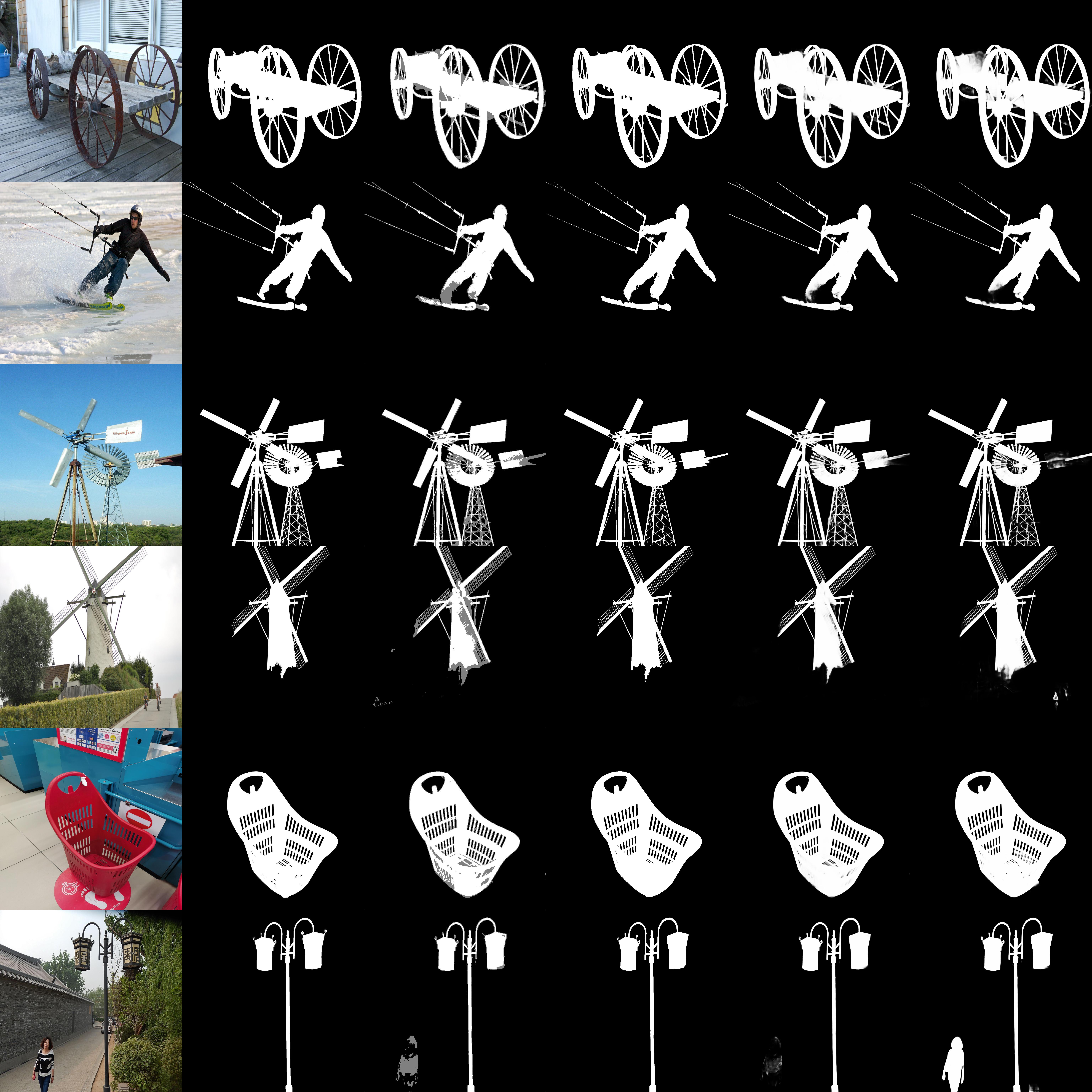
Input

GT

Confidence Trimap

BEN Base + Refiner

BEN Base

MVANet

Figure 2: Qualitative results from DIS5K validation

4.4 Quantitative Results

To intuitively understand how the refiner is updating the base predictions we selected outputs from the confidence trimap algorithm, BEN Base, and BEN Base + Refiner that are in the training dataset. As shown in Figure 2 the refiner is correctly able to remove and refine edges of the base models prediction. This combination significantly outperforms the MVANet as it is unable to correctly define foreground objects and attend to fine details.

5 Conclusion

In this paper, we examine the union of image foreground segmentation and image matting with the creation of BEN. We leverage CGM to allow the Refiner sufficient control over uncertain areas from BEN Base’s initial prediction. This powerful combination shows significant improvements over existing segmentation methods on the DIS5K validation dataset. Our work supports further exploration of confidence-based matting techniques in image segmentation.

6 References

Appendix A PyTorch Implementation of Confidence Trimap Generation

Basic PyTorch implementation of combined Algorithm 1 and Algorithm 2 is shown in Listing 1. This implementation provides an efficient vectorized version of the confidence trimap generation algorithm.

Listing 1: PyTorch Implementation of confidence trimap generation

⬇

1def generate_trimap(pred):

2 """

3 Generate a confidence-based trimap from a predicted mask.

4 Args:

5 pred: Predicted mask tensor

6 min_pixels: Minimum number of gray pixels required

7 Returns:

8 trimap: Generated trimap tensor

9 """

10 # Initialize thresholds

11

12 min_pixels=60000

13 t_high = 0.90

14 t_low = 0.10

15 t_min = 0.03 # Lower bound

16 t_max = 0.97 # Upper bound

17 step = 0.001 # Adjustment size

18 mask = pred.sigmoid() # Apply sigmoid to prediction

19

20 # Generate initial trimap

21 trimap = torch.where(

22 mask >= t_high,

23 mask.new_tensor(255.0),

24 torch.where(

25 mask <= t_low,

26 mask.new_tensor(0.0),

27 mask.new_tensor(128.0)

28 )

29 )

30

31 # Count gray pixels and adjust thresholds

32 n_gray = (trimap == 128).sum().item()

33 while n_gray < min_pixels:

34 t_low = max(t_low - step, t_min)

35 t_high = min(t_high + step, t_max)

36

37 if (t_low <= t_min and t_high >= t_max):

38 break # Exit if bounds reached

39

40 trimap = torch.where(

41 mask >= t_high,

42 trimap.new_tensor(255.0),

43 torch.where(

44 mask <= t_low,

45 trimap.new_tensor(0.0),

46 trimap.new_tensor(128.0)

47 )

48 )

49 n_gray = (trimap == 128).sum().item()

50

51 return trimap

References

- [1] Sungha Choi, Joanne T Kim, and Jaegul Choo. Cars can’t fly up in the sky: Improving urban-scene segmentation via height-driven attention networks. In Proceedings of the IEEE/CVF conference on computer vision and pattern recognition, pages 9373–9383, 2020.
- [2] Quang-Huy Che, Dinh-Phuc Nguyen, Minh-Quan Pham, and Duc-Khai Lam. Twinlitenet: An efficient and lightweight model for driveable area and lane segmentation in self-driving cars. In 2023 International Conference on Multimedia Analysis and Pattern Recognition (MAPR), pages 1–6. IEEE, 2023.
- [3] Junde Wu and Min Xu. One-prompt to segment all medical images. In Proceedings of the IEEE/CVF Conference on Computer Vision and Pattern Recognition (CVPR), pages 11302–11312, June 2024.
- [4] Xuzhe Zhang, Yuhao Wu, Elsa Angelini, Ang Li, Jia Guo, Jerod M. Rasmussen, Thomas G. O’Connor, Pathik D. Wadhwa, Andrea Parolin Jackowski, Hai Li, Jonathan Posner, Andrew F. Laine, and Yun Wang. Mapseg: Unified unsupervised domain adaptation for heterogeneous medical image segmentation based on 3d masked autoencoding and pseudo-labeling. In Proceedings of the IEEE/CVF Conference on Computer Vision and Pattern Recognition (CVPR), pages 5851–5862, June 2024.
- [5] Hao Ding, Changchang Sun, Hao Tang, Dawen Cai, and Yan Yan. Few-shot medical image segmentation with cycle-resemblance attention. In 2023 IEEE/CVF Winter Conference on Applications of Computer Vision (WACV), pages 2487–2496, 2023.
- [6] Xuebin Qin, Hang Dai, Xiaobin Hu, Deng-Ping Fan, Ling Shao, and Luc Van Gool. Highly accurate dichotomous image segmentation. In European Conference on Computer Vision, pages 38–56. Springer, 2022.
- [7] Qian Yu, Xiaoqi Zhao, Youwei Pang, Lihe Zhang, and Huchuan Lu. Multi-view aggregation network for dichotomous image segmentation. In Proceedings of the IEEE/CVF Conference on Computer Vision and Pattern Recognition, pages 3921–3930, 2024.
- [8] Ze Liu, Yutong Lin, Yue Cao, Han Hu, Yixuan Wei, Zheng Zhang, Stephen Lin, and Baining Guo. Swin transformer: Hierarchical vision transformer using shifted windows. In Proceedings of the IEEE/CVF international conference on computer vision, pages 10012–10022, 2021.
- [9] Alexey Dosovitskiy. An image is worth 16x16 words: Transformers for image recognition at scale. arXiv preprint arXiv:2010.11929, 2020.
- [10] Qian Yu, Peng-Tao Jiang, Hao Zhang, Jinwei Chen, Bo Li, Lihe Zhang, and Huchuan Lu. High-precision dichotomous image segmentation via probing diffusion capacity. arXiv preprint arXiv:2410.10105, 2024.
- [11] Diederik P Kingma. Auto-encoding variational bayes. arXiv preprint arXiv:1312.6114, 2013.
- [12] Robin Rombach, Andreas Blattmann, Dominik Lorenz, Patrick Esser, and Björn Ommer. High-resolution image synthesis with latent diffusion models. In Proceedings of the IEEE/CVF conference on computer vision and pattern recognition, pages 10684–10695, 2022.
- [13] Jingfeng Yao, Xinggang Wang, Shusheng Yang, and Baoyuan Wang. Vitmatte: Boosting image matting with pre-trained plain vision transformers. Information Fusion, 103:102091, 2024.
- [14] D Ulyanov. Instance normalization: The missing ingredient for fast stylization. arXiv preprint arXiv:1607.08022, 2016.
- [15] Dan Hendrycks and Kevin Gimpel. Gaussian error linear units (gelus). arXiv preprint arXiv:1606.08415, 2016.
- [16] Peng Zheng, Dehong Gao, Deng-Ping Fan, Li Liu, Jorma Laaksonen, Wanli Ouyang, and Nicu Sebe. Bilateral reference for high-resolution dichotomous image segmentation. arXiv preprint arXiv:2401.03407, 2024.
- [17] Federico Perazzi, Philipp Krähenbühl, Yael Pritch, and Alexander Hornung. Saliency filters: Contrast based filtering for salient region detection. In 2012 IEEE Conference on Computer Vision and Pattern Recognition, pages 733–740, 2012.
- [18] Ran Margolin, Lihi Zelnik-Manor, and Ayellet Tal. How to evaluate foreground maps? In Proceedings of the IEEE Conference on Computer Vision and Pattern Recognition (CVPR), June 2014.
- [19] Deng-Ping Fan, Ming-Ming Cheng, Yun Liu, Tao Li, and Ali Borji. Structure-measure: A new way to evaluate foreground maps. In Proceedings of the IEEE international conference on computer vision, pages 4548–4557, 2017.
- [20] Deng-Ping Fan, Cheng Gong, Yang Cao, Bo Ren, Ming-Ming Cheng, and Ali Borji. Enhanced-alignment measure for binary foreground map evaluation. arXiv preprint arXiv:1805.10421, 2018.
- [21] Reuben R Shamir, Yuval Duchin, Jinyoung Kim, Guillermo Sapiro, and Noam Harel. Continuous dice coefficient: a method for evaluating probabilistic segmentations. arXiv preprint arXiv:1906.11031, 2019.
- [22] Hamid Rezatofighi, Nathan Tsoi, JunYoung Gwak, Amir Sadeghian, Ian Reid, and Silvio Savarese. Generalized intersection over union: A metric and a loss for bounding box regression. In Proceedings of the IEEE/CVF conference on computer vision and pattern recognition, pages 658–666, 2019.
- [23] Tao Liu and Kai Yu. Ber: Balanced error rate for speaker diarization. arXiv preprint arXiv:2211.04304, 2022.
- [24] Taehun Kim, Kunhee Kim, Joonyeong Lee, Dongmin Cha, Jiho Lee, and Daijin Kim. Revisiting image pyramid structure for high resolution salient object detection. In Proceedings of the Asian Conference on Computer Vision, pages 108–124, 2022.
- [25] Guangkai Xu, Yongtao Ge, Mingyu Liu, Chengxiang Fan, Kangyang Xie, Zhiyue Zhao, Hao Chen, and Chunhua Shen. Diffusion models trained with large data are transferable visual models. arXiv preprint arXiv:2403.06090, 2024.