Nonisotropic Gaussian Diffusion for Realistic 3D Human Motion Prediction

Abstract

Probabilistic human motion prediction aims to forecast multiple possible future movements from past observations. While current approaches report high diversity and realism, they often generate motions with undetected limb stretching and jitter. To address this, we introduce SkeletonDiffusion, a latent diffusion model that embeds an explicit inductive bias on the human body within its architecture and training. Our model is trained with a novel nonisotropic Gaussian diffusion formulation that aligns with the natural kinematic structure of the human skeleton. Results show that our approach outperforms conventional isotropic alternatives, consistently generating realistic predictions while avoiding artifacts such as limb distortion. Additionally, we identify a limitation in commonly used diversity metrics, which may inadvertently favor models that produce inconsistent limb lengths within the same sequence. SkeletonDiffusion sets a new benchmark on three real-world datasets, outperforming various baselines across multiple evaluation metrics. Visit our project page.

1 Introduction

In this work, we address the problem of predicting human motion based on observed past movements, known as Human Motion Prediction (HMP). Specifically, from a temporal sequence of human joint positions, we aim to forecast their evolution in subsequent frames. HMP is a relevant problem for various real-world applications [90, 86, 87, 83, 84, 9, 45, 70, 36] and the key enabler of various downstream tasks [63, 3]: autonomous driving [59], healthcare [68], assistive robotics [41, 69], human-robot interaction [11, 14, 41, 27], and virtual reality or animation creation [72]. The task can be formulated as a deterministic regression by predicting the most likely future motion [53, 51, 18, 23, 35, 55, 26, 60, 46, 42, 57, 2, 12, 56, 28]. However, many applications [59, 63, 11, 14, 41, 27] require considering the inherent uncertainty of future movements. Stochastic Human Motion Prediction (SHMP) methods aim to learn a probability distribution over possible future motions. Once models are capable of representing multiple futures, the challenge lies in generating diverse yet realistic predictions. In our study, we observed that often diversity in the results comes at the cost of favoring physically unfeasible movements [5], such as velocity irregularities between frames (e.g., jittering or shaking) or inconsistent joint positions (e.g., changing bone lengths between frames). We believe this phenomenon to be a direct consequence of the lack of a proper inductive bias on the human skeletal structure. We present SkeletonDiffusion, a latent diffusion model encoding this bias explicitly on both architecture and training.

First, consider the skeleton structure and joint categories throughout the entire network and build our architecture on top of Typed-Graph Convolutions [65]. In contrast, existing SHMP approaches either ignore the skeleton’s graph structure [5, 90, 88, 16] or only leverage it at intermediate stages through Graph Convolutional Networks (GCNs)  [54, 19, 67, 80]. Second, we model the generative strategy to integrate the explicit bias. Similarly to the recent advances in SHMP based on diffusion models [5, 67, 16, 80], we opt for latent diffusion [62]. However, we replace the conventional isotropic Gaussian diffusion training [31] with a novel nonisotropic formulation that accounts for joint relations directly in the generation process: HMP is a structured problem defined by the skeleton kinematic graph, and we exploit this knowledge to define a fixed non-diagonal noise covariance for the diffusion process. To the best of our knowledge, this is the first nonisotropic diffusion process to support a non i.i.d. (i.i.d. = independent and identically distributed) latent space and reflect the problem structure. Despite demonstrating its usefulness in the skeletal domain, its applicability can be broader and touch all the domains where the conventional i.i.d. noise assumption may not hold due to the structural nature of the task.

We evaluate SkeletonDiffusion against the state-of-the-art on a large MoCap dataset (AMASS [52]), noisy data obtained by external camera tracking (FreeMan [79]), and in a zero-shot setting (3DPW [76]). We showcase consistently improved performance by generating realistic and diverse predictions (Fig. 1) with the least amount of stretching and jittering of bone lengths (body realism). In summary, our contributions are:

• We derive the first nonisotropic Gaussian diffusion formulation for a structural problem, which comprehends a detailed mathematical derivation and the required equations for training and inference.

• We propose SkeletonDiffusion, a novel latent diffusion model for SHMP that explicitly incorporates end-to-end the skeleton structure in the graph architecture and the diffusion training.

• We conduct extensive analyses and demonstrate SkeletonDiffusion’s state-of-the-art performance on multiple datasets. Our results demonstrate issues overlooked by previous methods (e.g., limbs’ stretching, jittering) and highlight the need for new realism and diversity metrics.

2 Related Work

2.1 Human Motion Prediction

Probabilistic HMP has been addressed via generative adversarial networks [7, 40, 47], variational autoencoders (VAE) [77, 85, 13, 54, 54, 25, 19, 88, 82], and more recently diffusion models [67, 16, 5, 64, 80]. Among these works, HumanMAC [16] and CoMusion [67] perform diffusion in input space, relying on a transformer backbone and representing the time dimension in Discrete Cosine Space (DCT), a temporal representation widely employed in SHMP [90, 54, 19, 80]. BeLFusion [5] performs latent diffusion [62] in a semantically meaningful latent space but by leveraging a U-Net [21]. We also wish to perform diffusion in latent space, due to its speed and generalization power [10]. Differently from deterministic HMP approaches [17, 44, 43], stochastic approaches leverage Graph Convolutional Networks (GCN) [39, 74] on the skeleton graph only at intermediate stages [54, 19, 67, 80]. In our method, we build on top of Typed-Graph Convolutions [65] and design a conditional autoencoder and denoising network. We later show how this is instrumental for our novel non-isotropic formulation.

2.2 Nonisotropic Probabilistic Diffusion Models

Diffusion models [31, 62] usually specify the noisification process through isotropic Gaussian random variables, sampling the noise for each diffusion step following the i.i.d. assumption. Recent studies [24, 15] show that the isotropic noise prior may not be the best choice for all tasks: optimizing the noise at inference time may improve result quality [22] or solve related tasks [37]. Few works in image generation explore non-Gaussian or learned alternatives, motivated by their efficiency [91, 50], or by addressing image corruption and inverse problems [20, 66]. When considering nonisotropic Gaussian processes [38, 32, 33, 75], the generated images are qualitatively comparable to the isotropic ones but retain longer training and inference time and less scalability [38, 32, 33]. We present a novel nonisotropic training formulation by modifying the covariance matrix of the noise addition, making the noisification process aware of joint connections. Since we rely on the known skeleton graph, the covariance matrix is not learned [91, 50] but fixed regardless of the input motion. While covariance matrices that depend on the input might not scale well with the problem size [33], our formulation is efficient and comes at no additional computational expenses during both training and inference. To the best of our knowledge, we are the first to apply nonisotropic Gaussian diffusion to a structured problem, also showing that our formulation converges with fewer iterations and parameters than its isotropic alternative (see Sup.Mat.).

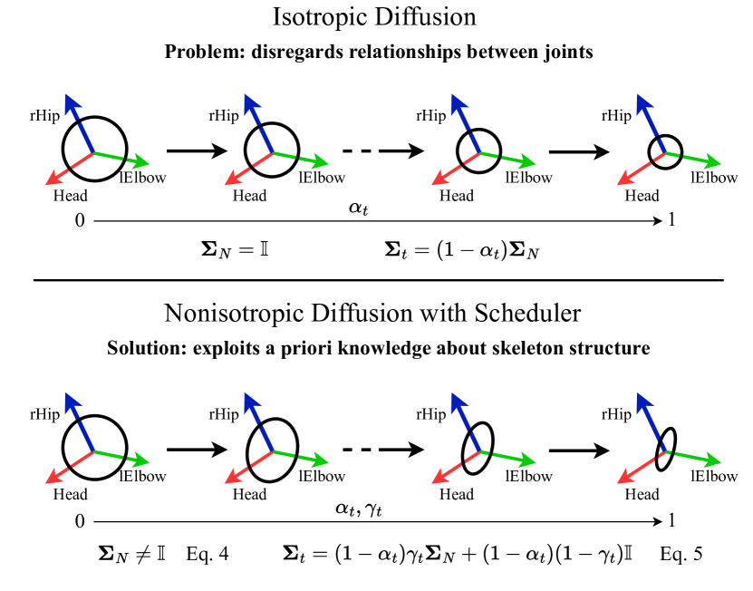
Figure 2: Our nonisotropic diffusion formulation. By diffusing a random variable ${\boldsymbol{x}}_{0}\in\mathbb{R}^{J}$ where $J$ is the number of body joints, instead of considering the joint dimensions i.i.d. as in isotropic diffusion, we take into account skeleton connections in $\boldsymbol{\Sigma}_{N}$. With the scheduler ${\gamma}_{t}$, we design a noise that transitions from isotropic to nonisotropic.

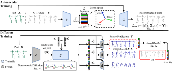
Figure 3: Overview of SkeletonDiffusion. We first train a conditional autoencoder, consisting of $\mathrm{{e}}$ and $\mathrm{{d}}$, to encode future human motions Y in a latent space $\boldsymbol{z}\in\mathbb{R}^{J\times L}$ where each of the $J$ latent joint dimensions corresponds to a human body joints. In this learned latent space, we train a denoiser network $\mathrm{{g}}$ with our novel nonisotropic diffusion formulation to generate latent embeddings ${\boldsymbol{x}}_{\theta}$ conditioned on the past X. During inference, the diffused samples are decoded to generate multiple diverse motions $\tilde{{\textbf{Y}}}$.

3 Preliminaries

3.1 Problem Formulation

The task of 3D Human Motion Prediction (HMP) takes as input a past sequence of $P$ poses and aims to predict the corresponding future as a sequence of $F$ poses. Formally, the input motion sequence is defined as $\textbf{X}=\left[{\textbf{p}}_{-P+1},{\textbf{p}}_{-P+2},\dots,{\textbf{p}}_{0}\right]\in\mathbb{R}^{P\times J\times 3}$, and the output motion sequence is defined as ${\textbf{Y}}=\left[{\textbf{p}}_{1},~\dots,~{\textbf{p}}_{F}\right]\in\mathbb{R}^{F\times J\times 3}$ with $J$ being the number of human body joints and ${\textbf{p}}_{\tau}$ the 3D body pose at timestep $\tau\in\{-P+1,-P+2,\dots,0,\dots,F\}$. Probabilistic or stochastic HMP considers a set of $N$ possible future sequences as $\tilde{{\textbf{Y}}}\in\mathbb{R}^{N\times F\times J\times 3}$ for each observation rather than a single deterministic prediction.

3.2 Isotropic Gaussian Diffusion

Diffusion generative models aim to learn the distribution $p({\boldsymbol{x}}_{0})$ of true data samples ${\boldsymbol{x}}_{0}$ by utilizing $T$ unseen hierarchical Markovian latent variables ${\boldsymbol{x}}_{1:T}$ of the same dimensions to define the prior $p({\boldsymbol{x}}_{T})$ and the posterior $q({\boldsymbol{x}}_{1:T}|{\boldsymbol{x}}_{0})$ distribution:

$$p({\boldsymbol{x}}_{0})=\frac{p({\boldsymbol{x}}_{0:T})}{q({\boldsymbol{x}}_{1:T}|{\boldsymbol{x}}_{0})}=\frac{p({\boldsymbol{x}}_{T})\prod_{t=1}^{T}p({\boldsymbol{x}}_{t-1}|{\boldsymbol{x}}_{t})}{\prod_{t=1}^{T}q({\boldsymbol{x}}_{t}|{\boldsymbol{x}}_{t-1})}.$$ (1)

Denoising Diffusion Probabilistic Models (DM) [31] define the forward transitions between latent random variables $p({\boldsymbol{x}}_{t}|{\boldsymbol{x}}_{t-1})$ as a linear Gaussian model $\mathcal{N}({\boldsymbol{x}}_{t};\sqrt{{\alpha}_{t}}{\boldsymbol{x}}_{t-1},{\boldsymbol{\Sigma}}_{t})$ with noise scheduler ${\alpha}_{t}$. This forward process iteratively transforms the initial variable ${\boldsymbol{x}}_{0}$ originating from the real data distribution $p({\boldsymbol{x}}_{0})$ into isotropic Gaussian noise $p({\boldsymbol{x}}_{T})=\mathcal{N}({\boldsymbol{x}}_{T};\boldsymbol{0},\mathbb{I})$. The reverse diffusion consists in sampling ${\boldsymbol{x}}_{T}\sim\mathcal{N}({\boldsymbol{x}}_{T};\boldsymbol{0},\mathbb{I})$ and iteratively applying the denoising transitions $q_{\theta}({\boldsymbol{x}}_{t-1}|{\boldsymbol{x}}_{t})$ parametrized by a neural network $\theta$ to obtain samples from the real data distribution, eventually with conditioning on other variables [5, 67] or modalities [62, 71]. These parameters are learned by maximizing the usual variational bound on log-likelihood [31, 48], derived from the closed form $p({\boldsymbol{x}}_{t}|{\boldsymbol{x}}_{0})$ of the forward transitions. Conventional isotropic diffusion defines the random variables ${\boldsymbol{x}}_{t}$ as i.i.d, i.e., as having a diagonal covariance matrix

$${\boldsymbol{\Sigma}}_{t}=(1-\alpha_{t})\mathbb{I}.$$ (2)

While Ho et al. [31] define the random variables in the input space, Latent Diffusion Models (LDM) [62, 71] reduce the dimensionality of the problem by considering lower-dimensional embeddings of the variables.

4 Method

We want to combine the generative capabilities of diffusion models with an explicit prior on realistic motions. This prior is obtained by embedding the knowledge about skeletal connections in both the network architecture and the training procedure. We present SkeletonDiffusion , a novel nonisotropic latent diffusion model where the noise addition is not i.i.d. but reflects limb connections. Here, we first present our nonisotropic diffusion formulation reflecting skeletal connections (Sec. 4.1) in a model-agnostic setting, and then introduce SkeletonDiffusion , implementing our nonisotropic training protocol with joint-attentive graph convolutional architecture (Sec. 4.2).

4.1 Nonisotropic Gaussian Diffusion

Clearly, in HMP every joint position depends on those of its neighbors. Relying on the i.i.d. noise assumption of conventional diffusion models [31, 62] would overlook such relations. Contrary to isotropic Gaussian diffusion that denoises all dimensions of random variables equally, we propose a nonisotropic formulation where the random variable ${\boldsymbol{x}}_{0}\in\mathbb{R}^{J}$ is denoised depending on the kinematic relations of a body with $J$ joints (Fig. 2).

Correlation Matrix $\boldsymbol{\Sigma}_{N}$

Since joint relationships are not dependent on the diffusion transition timestep $t$, we define our transition covariance matrix ${\boldsymbol{\Sigma}}_{t}$ in dependence of a correlation matrix $\boldsymbol{\Sigma}_{N}\in\mathbb{R}^{J\times J}$ encoding the skeleton structure:

$${\boldsymbol{\Sigma}}_{t}=(1-\alpha_{t})\boldsymbol{\Sigma}_{N}.$$ (3)

A natural choice for $\boldsymbol{\Sigma}_{N}$ seems the adjacency matrix $\mathbf{A}$ of the simple undirected graph originating from the body skeleton. However, $\mathbf{A}$ is an arbitrary matrix not guaranteed to be positive-definite, which is a fundamental property for covariance matrices. Furthermore, to avoid imbalances and exploding values in the noise, the magnitude of $\boldsymbol{\Sigma}_{N}$ should align with $\mathbb{I}$. To address these two constraints, we subtract the smallest eigenvalue $\lambda_{\text{min}}(\mathbf{A})$ from the diagonal elements and normalize the result to get the final $\boldsymbol{\Sigma}_{N}$:

$$\begin{split}\boldsymbol{\Sigma}_{N}=\frac{\mathbf{A}-\lambda_{\text{min}}(\mathbf{A})\mathbb{I}}{\lambda_{\text{max}}(\mathbf{A})-\lambda_{\text{min}}(\mathbf{A})}.\end{split}$$ (4)

In Sup.Mat., we ablate the choice of $\mathbf{A}$ against two different, more densely populated choices (the weighted transitive closure of the skeleton graph and its masked version). Our formulation comes with negligible computational expenses without loss of generalization and can be adapted to any structural problem with a suitable choice of $\mathbf{A}$.

Nonisotropic Covariance Scheduler

Although the simple solution presented in Eq. 3 is already superior to the isotropic diffusion (see Sec. 5.2), we observe that different diffusion timesteps $t$ relate to different aspects of the generation process. First, the network figures out high-level, global properties of the future motion, and later, fine-grained joints’ play a more significant role. With this motivation, we define a noise addition ${\boldsymbol{\Sigma}}_{t}$ that transitions from isotropic to nonisotropic noise:

$${\boldsymbol{\Sigma}}_{t}=(1-{\alpha}_{t}){\gamma}_{t}\boldsymbol{\Sigma}_{N}+(1-{\alpha}_{t})(1-{\gamma}_{t})\mathbb{I},$$ (5)

where ${\gamma}_{t}=1-t/T$ defines a monotonically decreasing scheduler. See details in the Sup.Mat.

Forward and Reverse Nonisotropic Diffusion

To avoid computing the noise at timestep $t$ in a recursive manner and effectively be able to perform training, we derive the closed-form $p({\boldsymbol{x}}_{t}|{\boldsymbol{x}}_{0})$ of the forward process

$${\boldsymbol{x}}_{t} =\sqrt{\bar{\alpha}_{t}}{\boldsymbol{x}}_{0}+\boldsymbol{U}\bar{\boldsymbol{\Lambda}}_{t}^{1/2}{\boldsymbol{\epsilon}},$$ (6)

where the nonisotropic noise is obtained from isotropic noise ${\boldsymbol{\epsilon}}\sim\mathcal{N}(\boldsymbol{0},\textbf{I})$ through the Eigendecomposition of the covariance matrix ${\boldsymbol{\Sigma}}_{t}=\boldsymbol{U}{\boldsymbol{\Lambda}}_{t}\boldsymbol{U}^{\top}$, with $\bar{\boldsymbol{\Lambda}}_{t}=\tilde{\gamma}_{t}{\boldsymbol{\Lambda}}_{t}+(1-\bar{\alpha}_{t})\mathbb{I}$, and $\tilde{\gamma}_{t}=(1-{\alpha}_{t}){\gamma}_{t}+{\alpha}_{t}\tilde{\gamma}_{t-1}$. To perform inference, we define a tractable form for the posterior $q({\boldsymbol{x}}_{t-1}|{\boldsymbol{x}}_{t})$ as

$$\begin{split}{\boldsymbol{x}}_{t-1}=&{\boldsymbol{\mu}}_{q}+\boldsymbol{U}{\boldsymbol{\Lambda}}_{q}{\boldsymbol{\epsilon}}\\ {\boldsymbol{\Lambda}}_{q}=&{\boldsymbol{\Lambda}}_{t}\bar{\boldsymbol{\Lambda}}_{t-1}\bar{\boldsymbol{\Lambda}}_{t}^{-1}\\ {\boldsymbol{\mu}}_{q}=&\sqrt{{\alpha}_{t}}\boldsymbol{U}\bar{\boldsymbol{\Lambda}}_{t}^{-1}\bar{\boldsymbol{\Lambda}}_{t-1}\boldsymbol{U}^{\top}{\boldsymbol{x}}_{t}\\ &+\sqrt{\bar{\alpha}_{t-1}}\boldsymbol{U}\bar{\boldsymbol{\Lambda}}_{t}^{-1}{\boldsymbol{\Lambda}}_{t}\boldsymbol{U}^{\top}{\boldsymbol{x}}_{0}\\ \end{split}$$ (7)

		Precision		Multimodal GT			Diversity	Realism	Body Realism
Type	Method								mean $\downarrow$		RMSE $\downarrow$
		ADE $\downarrow$	FDE $\downarrow$	MMADE $\downarrow$	MMFDE $\downarrow$	APDE $\downarrow$	APD $\uparrow$	CMD $\downarrow$	str	jit	str	jit
Alg	Zero-Velocity	0.755	0.992	0.814	1.015	-	0.000	39.262	0.00	0.00	0.00	0.00
VAE	TPK [77]	0.656	0.675	0.658	0.674	2.265	9.283	17.127	7.34	0.34	9.69	0.48
	DLow [88]	0.590	0.612	0.618	0.617	4.243	13.170	15.185	8.41	0.40	11.06	0.58
	GSPS [54]	0.563	0.613	0.609	0.633	4.678	12.465	18.404	6.65	0.29	8.98	0.37
	DivSamp [19]	0.564	0.647	0.623	0.667	15.837	24.724	50.239	11.17	0.82	16.71	1.0
DM	HumanMAC [16]	0.511	0.554	0.593	0.591	-	9.321	-	-	-	-	-
	BeLFusion [5]	0.513	0.560	0.569	0.585	1.977	9.376	16.995	7.19	0.34	9.03	0.34
	CoMusion [67]	0.494	0.547	0.469	0.466	2.328	10.848	9.636	4.04	0.25	5.63	0.52
DM	SkeletonDiffusion (Ours)	0.480	0.545	0.561	0.580	2.067	9.456	11.417	3.15	0.20	4.45	0.26

Table 1: Quantitative results for AMASS dataset [52]. The best results are highlighted in bold, second-best are underlined. The symbol ‘-’ indicates that the results are not reported in the baseline work. We achieve state-of-the-art performance, while the VAE-based method with the highest diversity, DivSamp, displays the worst limb stretching and limb jitter.

4.2 SkeletonDiffusion

SkeletonDiffusion is an LDM composed of a conditional autoencoder and a denoiser network, trained in two different stages (Fig. 3). First, we train the autoencoder to reconstruct future motions Y by encoding them in the latent space $\boldsymbol{z}=\mathrm{{e}}({\textbf{Y}})\in\mathbb{R}^{J\times L}$ and decoding them conditioning on the last two observation frames as $\mathrm{{d}}(\boldsymbol{z},\textbf{X}_{-2:0})$. After, the denoiser network $\mathrm{{g}}$ learns with our nonisotropic diffusion to denoise true latent variables $\boldsymbol{z}$ conditioned on past observations $\mathrm{{e}}(\textbf{X})$. At inference, we recover multiple latent codes ${\boldsymbol{x}}_{\theta}$ by sampling and denoising isotropic Gaussian noise and decode them into future predictions $\tilde{{\textbf{Y}}}$.

Latent Representation

While our nonisotropic diffusion has been defined in Sec. 4.1 to operate on $\boldsymbol{z}\in\mathbb{R}^{J}$, we aim for a richer latent representation, capable of encoding the complex temporal information. Hence, we opt for a two-dimensional latent representation $\boldsymbol{z}\in\mathbb{R}^{J\times L}$ where every $j$-th body joint is described by a vector of dimension $L$. Notice that the latent feature dimension $L$ does not explicitly encode information between joints. Thus we assume i.i.d noise over this dimension and perform nonisotropic diffusion only along the $J$ one. Similar latent configurations have been shown effective in other domains, e.g., in image generation [62], but have not been applied to HMP before. In Sup.Mat., we show the correlation of the latent joint dimensions through PCA.

Joint-Attentive GCN

We advocate for an architecture that performs attention on the skeleton joints [65] from end to end throughout the whole model and opt for Typed-Graph (TG) Convolutions [65]. For a TG layer taking as input features ${\boldsymbol{x}}\in\mathbb{R}^{J\times D_{in}}$, we define a feature extraction matrix $\mathbf{W}^{j}\in\mathbb{R}^{D_{in}\times D_{out}}$ for each joint $j$ with shared weights depending on the specific joint, and a feature aggregation matrix $\mathbf{G}\in\mathbb{R}^{J\times J}$. The features $\mathbf{f}\in\mathbb{R}^{J\times D_{out}}$ are first extracted for each joint $j$ independently through

$$\mathbf{f}=\mathbf{G}\cdot\hat{\mathbf{f}},\,\text{with}\,\,\hat{\mathbf{f}}^{j}=\mathbf{W}^{j}\cdot{\boldsymbol{x}}^{j}$$ (8)

and then aggregated. We further define the TG version of multi-head self-attention [73] as Typed-Graph Attention (TG-Attention). By obtaining and aggregating the query, key, and value matrices through TG layers, we apply the self-attention mechanism on a joint level (equations in Sup.Mat.). Both encoder and decoder are TG-GRUs [65], exploiting the convenient inductive biases of recurrent neural networks (RNNs) for motion modeling [49]. The denoiser network is designed as a TG-Attention network with residual connections. In this way, we define a fully TG architecture that preserves the body joint dimensions continuously throughout the whole architecture.

Training Objective

First, the conditional autoencoder is trained to encode and reconstruct future motions according to the autoencoder objective:

$$L_{\mathrm{autoenc}}=L_{\mathrm{rec}}(\mathrm{{e}}({\textbf{Y}}),{\textbf{Y}},\textbf{X}),$$ (9)

where the reconstruction loss is defined as

$$L_{\mathrm{rec}}(\boldsymbol{z},{\textbf{Y}},\textbf{X}):=\|\mathrm{{d}}(\boldsymbol{z},\textbf{X}_{-2:0})-{\textbf{Y}}\|_{1}.$$ (10)

Here the conditioning on the past encourages smooth transitions between past and future motions. More details on the first training stage can be found in Sup.Mat. After the first training stage, the learned latent joint dimensions exhibit correlations similar to skeleton body joints - this is the foundation of our nonisotropic diffusion training. In the second training stage, the denoising network $\mathrm{{g}}$ learns to reverse this noisification process. Instead of predicting the noise ${\boldsymbol{\epsilon}}_{t}$ [31, 62], we aim to directly approximate the true latent code ${\boldsymbol{x}}_{0}:=\boldsymbol{z}$ [61, 5] as ${\boldsymbol{x}}_{\boldsymbol{\theta}}=\mathrm{{g}}({\boldsymbol{x}}_{t},\mathrm{{e}}(\textbf{X}),t)$. The diffusion loss can be formulated as a Mahalanobis distance:

$$L_{\mathrm{diff}}({\boldsymbol{x}}_{\boldsymbol{\theta}},{\boldsymbol{x}}_{0},t):=\bar{\alpha}_{t}\|\bar{\boldsymbol{\Lambda}}_{t}^{-1/2}\boldsymbol{U}^{\top}({\boldsymbol{x}}_{\boldsymbol{\theta}}-{\boldsymbol{x}}_{0})\|^{2},$$ (11)

To implicitly enforce diversity [5, 67, 29], we relax Eq. (11) by sampling $k=50$ predictions at each iteration and backpropagating the gradient only through the prediction that minimizes the loss.

$$\hskip-3.1298ptL_{\mathrm{gen}}=\mathbb{E}_{{\textbf{Y}},\textbf{X},t}L_{\mathrm{diff}}(\arg\min_{k}L_{\mathrm{rec}}({\boldsymbol{x}}_{\boldsymbol{\theta}}^{k},{\textbf{Y}},\textbf{X}),\mathrm{{e}}({\textbf{Y}}),t)$$ (12)

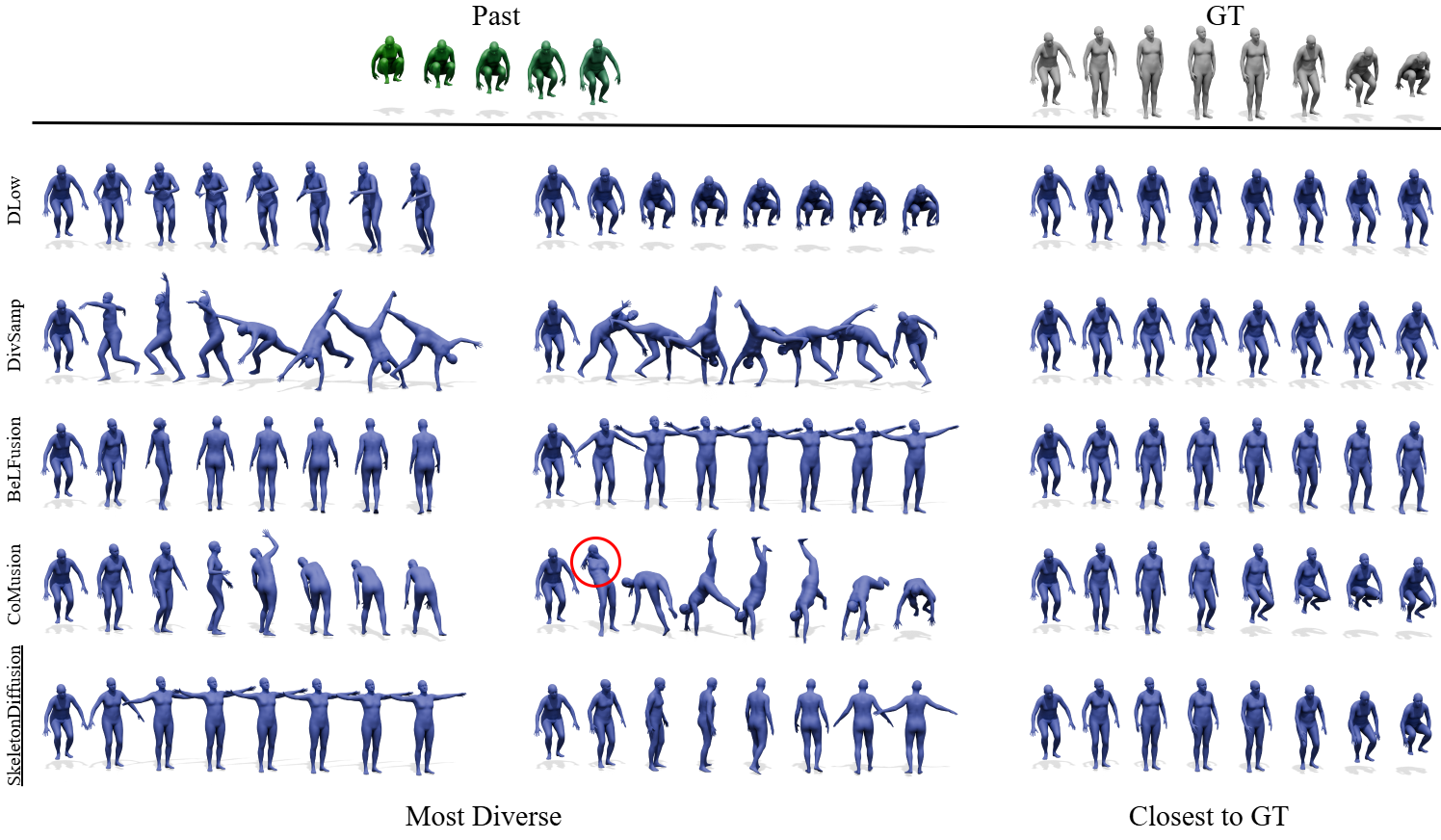
Figure 4: Qualitative Results on AMASS. On top, we report the input past observation and the ground-truth future. For every method, we report the closest prediction to GT according to ADE on the right and the two furthermost predictions on the two left-most columns. Our closest competitors generate realistic motions but do not include a motion close to the GT (BeLFusion) or diverse predictions, and present evident unrealistic artifacts (CoMusion). Our method is the only one to produce realistic and diverse motions.

5 Experiments

5.1 Experimental Settings

Baselines

We compare SkeletonDiffusionwith state-of-the-art approaches [67, 5, 16, 19, 77, 88, 54] and include the ZeroVelocity baseline, competitive in HMP [55, 4] by simply outputting the last seen pose for every future timestep.

Datasets

We evaluate on the large-scale dataset AMASS [52] according to the cross-dataset evaluation protocol [5, 67]. We aim to test SHMP methods with real-world data obtained not from MoCap but from noise sources (e.g., RGB cameras, and sparse IMUs). To this end, we perform zero-shot experiments on 3D Poses in the Wild (3DPW)[76] for available models trained on AMASS, and adapt the recent in-the-wild, large-scale dataset FreeMan[79] to the motion prediction task and retrain on it various state-of-the-art methods. Compared to AMASS, we deem the conventionally employed Human3.6M dataset [34] less representative (only 7 subjects) and discuss it directly in Sup.Mat. with further details. As in previous works, we predict the next 2s into the future from observations of 0.5s.

Metrics and Body Realism

Recent SHMP works concentrate on four factors: precision, coverage of the ground truth test distribution (multimodal metrics), diversity, and realism. We consider conventionally employed metrics [88, 5] and report their definition and discussion in Sup.Mat.

It is worth noting that while the CMD metric addresses realism, it is solely expressed in terms of joint velocities. The actual Body realism, e.g., bone lengths preservation along the motion, although crucial for meaningful predictions, is overlooked. Even worse, a consequence of artifacts such as changes in limb lengths over the timespan (limbs stretching) and frequent inconsistencies between consecutive frames (limbs jitter) impact other metrics, for example, by causing more diversity in the predictions, and so higher APD value (see Sup.Mat. for further discussion). This motivates us to investigate this aspect and propose novel metrics. Given a future ground truth sequence Y with $\mathrm{B}$ limbs (or bones) and a predicted sequence $\tilde{{\textbf{Y}}}$, for each frame $\tau$ of the prediction associated pose $\tilde{\textbf{p}}_{\tau}$, we denote the length of the $j$-th limb as $\tilde{b}^{j}_{\tau}\in\mathbb{R}$. We define the normalized $j$-th limb length error $e^{j}_{\tau}$ and limb jitter $v^{j}_{\tau}$ at a time $\tau$ as:

$$e^{j}_{\tau}:=\frac{1}{b^{j}}\left|b^{j}-\tilde{b}^{j}_{\tau}\right|,\quad v^{j}_{\tau}:=\frac{1}{b^{j}}\left|\tilde{b}^{j}_{\tau+1}-\tilde{b}^{j}_{\tau}\right|$$ (13)

where $b^{j}\in\mathbb{R}$ is the ground truth length of the $j$-th limb. By calculating the mean and root mean square error (RMSE) of these two vectors over the time dimension, we define four body realism metrics: mean for stretching str and jitter jit, and analogously RMSE.

	Precision		Multimodal GT		Diversity	Realism	Body Realism
Method							mean $\downarrow$		RMSE $\downarrow$
	ADE $\downarrow$	FDE $\downarrow$	MMADE $\downarrow$	MMFDE $\downarrow$	APD $\uparrow$	CMD $\downarrow$	str	jit	str	jit
HumanMAC [16]	0.415	0.511	0.537	0.600	5.426	2.025	7.91	1.49	11.89	1.84
BeLFusion [5]	0.420	0.495	0.496	0.516	5.209	6.306	10.46	0.41	11.93	0.54
CoMusion [67]	0.389	0.480	0.527	0.525	6.687	2.764	7.94	0.81	10.27	1.053
SkeletonDiffusion (Ours)	0.374	0.457	0.506	0.508	6.732	3.166	7.58	0.51	9.64	0.66

Table 2: Quantitative results on FreeMan [79]. The best results are highlighted in bold, second best are underlined. SkeletonDiffusionachieves the best precision and diversity on noisy real-world data while maintaining consistent body realism.

5.2 Results

Large-scale Evaluation on AMASS

Following the cross-dataset evaluation protocol of BelFusion [5], we train on a subset of datasets belonging to AMASS and test on others. We report our results in Tab. 1. Starting from the conventional metrics evaluation, our method already achieves state-of-the-art performance on the majority of the metrics, with a significant improvement on precision. Among other Diffusion-based methods (DM), SkeletonDiffusion and CoMusion contend with each other for first and second place according to diversity, realism, and multimodal metrics. Although VAE-methods tend to show higher diversity, as already mentioned by previous works [5, 16], the high diversity values of [82, 88] may often be the consequence of unrealistic motions with irregularities between past and future or inconsistent speed. From the qualitative example reported in Fig. 4, we notice that both the most diverse predictions of DivSamp represent a cartwheeling motion. While such motions may geometrically be diverse from each other and thus increase the APD, they are not only not semantically diverse but also not consistent with the past observation.

Body Realism and Diversity

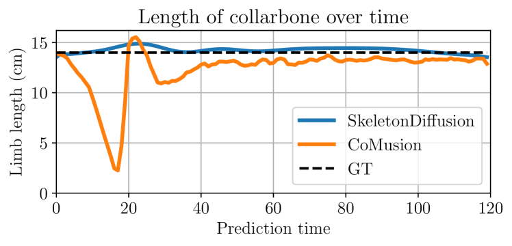
Figure 5: A qualitative example of collarbone bone length evolution for a single predicted motion from AMASS. SkeletonDiffusion keeps the bone length consistent over time and close to the GT, while CoMusion shows inconsistencies of large magnitude.

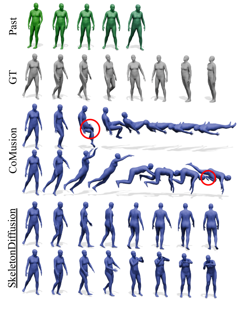
Figure 6: Qualitative results of zero-shot on 3DPW [76] for models trained on AMASS[52]. CoMusion displays limb twisting, while our predictions are realistic and consistent.

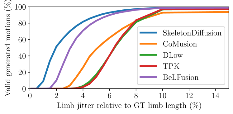
Figure 7: Motions’ validity on different error tolerance on AMASS. For every method, we show the evolution of valid motions quantity (y-axis) for which the maximal error is below a given threshold (x-axis). SkeletonDiffusion presents consistently the highest number of valid poses. CoMusion and VAE methods cannot generate predictions with an error lower than 2.5%.

		Precision		Multimodal GT		Diversity	Realism	Body Realism
Type	Method							mean $\downarrow$		RMSE $\downarrow$
		ADE $\downarrow$	FDE $\downarrow$	MMADE $\downarrow$	MMFDE $\downarrow$	APD $\uparrow$	CMD $\downarrow$	str	jit	str	jit
VAE	TPK [77]	0.648	0.701	0.665	0.702	9.582	13.136	7.61	0.36	10.02	0.51
	DLow [88]	0.581	0.649	0.602	0.651	13.772	11.977	8.53	0.42	11.28	0.61
	GSPS [54]	0.552	0.650	0.578	0.653	11.809	12.722	6.38	0.29	8.65	0.35
	DivSampling [19]	0.554	0.678	0.593	0.686	24.153	46.431	11.04	0.78	16.31	1.01
DM	BeLFusion [5]	0.493	0.590	0.531	0.599	7.740	17.725	6.47	0.22	7.96	0.29
	CoMusion	0.477	0.570	0.540	0.587	11.404	7.093	4.01	0.38	5.54	0.50
DM	SkeletonDiffusion (Ours)	0.472	0.575	0.535	0.594	9.814	10.474	3.02	0.17	4.16	0.23

Table 3: Zero-Shot evaluation on 3DPW [76] for models trained on AMASS[52]. The best results are highlighted in bold, second best are underlined. While CoMusion’s limb jitter worsens, we present the highest body realism accompanied by solid performance.

On the right-most part of Tab. 1, we analyze limb stretching and jittering in the methods’ predictions with our body realism metrics. First, this issue particularly affects VAE approaches, and the two methods with the highest APD are also the two with the largest errors on all four metrics. This supports our intuition that diversity may benefit from artifacts and inconsistencies. SkeletonDiffusion presents the best metrics by a large margin, highlighting the contribution of our prior on the skeleton structure. CoMusion displays much worse body realism and is the third worst in terms of RMSE error for the jittering. We qualitatively visualize the inconsistency of a limb (the collarbone) for a sequence in Fig. 5, reporting its length variation over time. Compared to the ground-truth length (the dashed line), CoMusion shows drastic changes already in the early frames. SkeletonDiffusion is much more consistent over time, remaining quite close to the real length. Finally, we stress the impact of such bone artifacts by considering the case in which an application has a hard requirement about the maximal admitted error for a sequence. Namely, if a sequence faces a bone stretching above a given threshold, it is considered unreliable and so discarded. In Fig. 7, we report how the number of valid sequences evolves on AMASS in dependence of such threshold, showing that our method is the most robust while CoMusion performs worst among DM models.

Noisy Data and FreeMan Dataset

We test for the first time SHMP methods on noisy data acquired from an external RGB camera from the FreeMan dataset[79]. In this case, GT poses reach a change in limb length up to 5.6cm, compared to close to zero of the AMASS MoCap setting. Our method achieves the best performance in precision and diversity and, at the same time, achieves the lowest limb stretching. This hints that SkeletonDiffusion  has effectively learned basic properties of the human skeletal structure achieving robustness to unprecise data. We report the evaluation results in Tab. 2. On the contrary, BelFusion achieves the worst CMD and limb length variation, showing that their bones increase length consistently over the whole prediction. Our findings highlight the informativeness of our four body realism metrics and how our design choices make SkeletonDiffusion  ready also for data sources not previously considered.

	ADE $\downarrow$	FDE $\downarrow$	MMADE $\downarrow$	MMFDE $\downarrow$	APD $\uparrow$
w/o TG-att	0.502	0.567	0.576	0.597	8.021
iso	0.499	0.553	0.568	0.583	8.788
noniso	0.489	0.547	0.566	0.581	9.483
ours	0.480	0.545	0.561	0.580	9.456

Table 4: Ablations on the AMASS dataset [52].

Zero-Shot Generalization on 3DPW

We are also interested in evaluating how SkeletonDiffusion  generalizes to out-of-distribution motions. Hence, we test the methods trained on AMASS on unseen, real-life scenes from 3DPW[76] and report results in Tab. 3. We notice that, while CoMusion’s limb jitter between consecutive frames has worsened in the zero-shot setting, our method shows solid results and consistently the best body realism. We report a qualitative example in Fig. 6. CoMusion’s predictions appear diverse but present low semantic consistency with the input past. Furthermore, both predictions are humanly feasible as they present limb twisting or excessive bending.

Ablations

In Tab. 4, we ablate the main components of SkeletonDiffusion on AMASS. We compare the effect of TG-Attention layers on isotropic diffusion ($\boldsymbol{\Sigma}_{N}=I$ and ${\gamma}_{t}=0$) and analyze nonisotropic diffusion with our covariance reflecting joint connections $\boldsymbol{\Sigma}_{N}$ (Eq. 4) in the variant where ${\gamma}_{t}=1$ (as in Eq. 3) and our blending with the scheduler ${\gamma}_{t}$ (Eq. 5). We see that our TG-Attention layers already improve the TG-CNN architecture in the conventional isotropic diffusion paradigm. While the simple nonisotropic variant achieves state-of-the-art performance (see Tab. 1), our formulation with the scheduler ${\gamma}_{t}$ further improves the metrics and in particular, precision. Ablation results regarding the choice of connectivity matrix for $\boldsymbol{\Sigma}_{N}$ and its normalization are reported in the Sup.Mat., where we also show that our nonisotropic formulation requires fewer parameters and training epochs than the isotropic one.

6 Conclusion

We present SkeletonDiffusion, a new latent diffusion model with an explicit inductive bias on the human skeleton trained with a novel nonisotropic Gaussian diffusion formulation. We achieve state-of-the-art performance on stochastic HMP by generating motions that are simultaneously realistic and diverse while being robust to limb stretching according to the evaluation metrics.

Limitations and Future Work

Similar to previous methods, we restrict our experiments to standard human skeletons, where fine-grained joints (e.g., fingers, facial expression) are not considered. Unfortunately, at the present date, such data are scarce and difficult to capture. Applying our non-isotropic diffusion on skeletons with more expressive structures is an inspiring direction for future works. We also believe it may be worth experimenting with different definitions of $\boldsymbol{\Sigma}_{N}$, depending on the applicative context, and eventually exploring non-Gaussian diffusion formulations.

Acknowledgments

This work was supported by the ERC Advanced Grant SIMULACRON. Thanks to Dr. Almut Sophia Koepke, Yuesong Shen and Shenhan Qian for the proofreading and feedback, Lu Sang for the discussion, Stefania Zunino and the whole CVG team for the support.

Supplementary Material

Appendix A Mathematical Derivations of our Nonisotropic Gaussian Diffusion

A.1 Forward Diffusion Process

As mentioned in the main paper body, the Gaussian forward transitions are defined as:

$$q({\boldsymbol{x}}_{t}|{\boldsymbol{x}}_{t-1})=\mathcal{N}({\boldsymbol{x}}_{t};\sqrt{{\alpha}_{t}}{\boldsymbol{x}}_{t-1},\boldsymbol{U}{\boldsymbol{\Lambda}}_{t}\boldsymbol{U}^{\top}).$$ (14)

allowing us to sample from a transition in dependence of isotropic noise ${\boldsymbol{\epsilon}}_{t}$ as:

$${\boldsymbol{x}}_{t}=\sqrt{{\alpha}_{t}}{\boldsymbol{x}}_{t-1}+\boldsymbol{U}{\boldsymbol{\Lambda}}_{t}^{1/2}{\boldsymbol{\epsilon}}_{t},$$ (15)

We can further derive the tractable form of the forward transitions $q({\boldsymbol{x}}_{t}|{\boldsymbol{x}}_{0})$ by recursively applying ${\boldsymbol{x}}_{t-1}=\sqrt{{\alpha}_{t-1}}{\boldsymbol{x}}_{t-2}+\boldsymbol{U}{\boldsymbol{\Lambda}}_{t-1}^{1/2}{\boldsymbol{\epsilon}}_{t-1}$:

$${\boldsymbol{x}}_{t}= \sqrt{{\alpha}_{t}}(\sqrt{{\alpha}_{t-1}}{\boldsymbol{x}}_{t-2}+\boldsymbol{U}{\boldsymbol{\Lambda}}_{t-1}^{1/2}{\boldsymbol{\epsilon}}_{t-1})+\boldsymbol{U}{\boldsymbol{\Lambda}}_{t}^{1/2}{\boldsymbol{\epsilon}}_{t}$$ (16)

$$= \sqrt{{\alpha}_{t}}(\sqrt{{\alpha}_{t-1}}(\sqrt{{\alpha}_{t-2}}{\boldsymbol{x}}_{t-3}$$

$$+\boldsymbol{U}{\boldsymbol{\Lambda}}_{t-2}^{1/2}{\boldsymbol{\epsilon}}_{t-2})+\boldsymbol{U}{\boldsymbol{\Lambda}}_{t-1}^{1/2}{\boldsymbol{\epsilon}}_{t-1})+\boldsymbol{U}{\boldsymbol{\Lambda}}_{t}^{1/2}{\boldsymbol{\epsilon}}_{t}$$

$$= \dots$$

$$= \sqrt{\bar{\alpha}_{t}}{\boldsymbol{x}}_{0}+\boldsymbol{U}\bar{\boldsymbol{\Lambda}}_{t}^{1/2}{\boldsymbol{\epsilon}}_{0}$$

$$\sim \mathcal{N}(\sqrt{\bar{\alpha}_{t}}{\boldsymbol{x}}_{0},\boldsymbol{U}(\bar{\boldsymbol{\Lambda}}_{t})\boldsymbol{U}^{T})=\mathcal{N}(\sqrt{\bar{\alpha}_{t}}{\boldsymbol{x}}_{0},\bar{\boldsymbol{\Sigma}}_{t}),$$

where we exploit the fact that the isotropic noises can be formulated as ${\boldsymbol{\epsilon}}_{t-1}\sim\mathcal{N}(\boldsymbol{0},{\alpha}_{t}\boldsymbol{U}{\boldsymbol{\Lambda}}_{t-1}\boldsymbol{U}^{T})$, ${\boldsymbol{\epsilon}}_{t}\sim\mathcal{N}(\boldsymbol{0},\boldsymbol{U}{\boldsymbol{\Lambda}}_{t}\boldsymbol{U}^{T})$ and that the sum of two independent Gaussian random variables is a Gaussian with mean equals the sum of the two means and the variance being the sum of the two variances. We have thus derived the Gaussian form of the tractable forward diffusion process $q({\boldsymbol{x}}_{t}|{\boldsymbol{x}}_{0})=\mathcal{N}(\sqrt{\bar{\alpha}_{t}}{\boldsymbol{x}}_{0},\boldsymbol{U}\bar{\boldsymbol{\Lambda}}_{t}\boldsymbol{U}^{T})$ for

$$\bar{\boldsymbol{\Lambda}}_{t}=\tilde{\gamma}_{t}{\boldsymbol{\Lambda}}_{\mathbb{I}}+(1-\bar{\alpha}_{t})\mathbb{I}$$ (17)

$$\tilde{\gamma}_{t}= \sum_{i=0}^{t}\bar{\gamma}_{t-i}{\alpha}_{t-i}^{-1}\prod_{j=t-i}^{t}{\alpha}_{j}$$ (18)

$$= \bar{\alpha}_{t}\sum_{i=0}^{t}\frac{\bar{\gamma}_{t-i}}{\bar{\alpha}_{t-i}}=\bar{\gamma}_{t}+{\alpha}_{t}\tilde{\gamma}_{t-1}\,.$$

A.2 Reverse Diffusion Process

To perform inference, we need to find a tractable form for the posterior $q({\boldsymbol{x}}_{t-1}|{\boldsymbol{x}}_{t},{\boldsymbol{x}}_{0})$ in terms of ${\boldsymbol{x}}_{0}$. With the forms of the Gaussian transitions, through Bayes rule

$$q({\boldsymbol{x}}_{t-1}|{\boldsymbol{x}}_{t},{\boldsymbol{x}}_{0})=\frac{q({\boldsymbol{x}}_{t}|{\boldsymbol{x}}_{t-1},{\boldsymbol{x}}_{0})q({\boldsymbol{x}}_{t-1}|{\boldsymbol{x}}_{0})}{q({\boldsymbol{x}}_{t}|{\boldsymbol{x}}_{0})}$$ (19)

we can start the derivation of the posterior $\mathcal{N}({\boldsymbol{x}}_{t-1};{\boldsymbol{\mu}}_{q},{\boldsymbol{\Sigma}}_{q})$ from

$$\frac{\mathcal{N}({\boldsymbol{x}}_{t};\sqrt{{\alpha}_{t}}{\boldsymbol{x}}_{t-1},{\boldsymbol{\Sigma}}_{t})\mathcal{N}({\boldsymbol{x}}_{t-1};\sqrt{\bar{\alpha}_{t-1}}{\boldsymbol{x}}_{0},\bar{\boldsymbol{\Sigma}}_{t-1})}{\mathcal{N}({\boldsymbol{x}}_{t};\sqrt{\bar{\alpha}_{t}}{\boldsymbol{x}}_{0},\bar{\boldsymbol{\Sigma}}_{t})}.$$ (20)

Differently from the conventional isotropic diffusion derivation, where this and subsequent derivations are carried out for scalar variables thanks to the i.i.d. assumption, our random variables are correlated and we have to deal with vectorial equations. Hence the posterior mean ${\boldsymbol{\mu}}_{q}$ and covariance ${\boldsymbol{\Sigma}}_{q}$ cannot be derived straightforwardly.

To address this issue, we exploit the eigenvalue decomposition of ${\boldsymbol{\Sigma}}_{t}$ and notice that the orthogonal matrix $\boldsymbol{U}$ is a linear transformation preserving the inner product of vectors by definition, and that thus the shape of the posterior probability distribution $q({\boldsymbol{x}}_{t-1}|{\boldsymbol{x}}_{t})$ stays the same in the isometry of the Euclidean space given

$$\tilde{\boldsymbol{x}}_{i}=\boldsymbol{U}^{\top}{\boldsymbol{x}}_{i}\,.$$ (21)

This allows us to ’rotate’ the posterior distribution $q({\boldsymbol{x}}_{t-1}|{\boldsymbol{x}}_{t})$ by the transformation $\boldsymbol{U}$ and carry out the derivation for a distribution $q(\tilde{\boldsymbol{x}}_{t-1}|\tilde{\boldsymbol{x}}_{t})=\mathcal{N}(\tilde{\boldsymbol{x}}_{t-1};\tilde{\boldsymbol{\mu}}_{q},{\boldsymbol{\Lambda}}_{q})$ that now has a diagonal covariance matrix ${\boldsymbol{\Lambda}}_{q}=\boldsymbol{U}^{\top}{\boldsymbol{\Sigma}}_{q}\boldsymbol{U}$. Now we can handle each dimension independently, since the matrices in the following derivations are diagonal matrices and this allows us to use the commutative property ${\boldsymbol{\Lambda}}_{1}{\boldsymbol{\Lambda}}_{2}={\boldsymbol{\Lambda}}_{2}{\boldsymbol{\Lambda}}_{1}$. In the following, we also make use of the observation:

$$\bar{\boldsymbol{\Lambda}}_{t}= {\alpha}_{t}\bar{\boldsymbol{\Lambda}}_{t-1}+{\boldsymbol{\Lambda}}_{t}$$ (22)

The mean and variance of the posterior can thus be derived in the isometry space as

$$q(\tilde{\boldsymbol{x}}_{t-1}|\tilde{\boldsymbol{x}}_{t}, \tilde{\boldsymbol{x}}_{0})$$ (23)

$$\begin{split}\propto\exp{}-\frac{1}{2}&\Big{[}(\tilde{\boldsymbol{x}}_{t}-\sqrt{{\alpha}_{t}}\tilde{\boldsymbol{x}}_{t-1})^{\top}{\boldsymbol{\Lambda}}_{t}^{-1}(\tilde{\boldsymbol{x}}_{t}-\sqrt{{\alpha}_{t}}\tilde{\boldsymbol{x}}_{t-1})\Big{.}\\ +(&\tilde{\boldsymbol{x}}_{t-1}-\sqrt{\bar{\alpha}_{t-1}}\tilde{\boldsymbol{x}}_{0})^{\top}\bar{\boldsymbol{\Lambda}}_{t-1}^{-1}(\tilde{\boldsymbol{x}}_{t-1}-\sqrt{\bar{\alpha}_{t-1}}\tilde{\boldsymbol{x}}_{0})\\ &\Big{.}-(\tilde{\boldsymbol{x}}_{t}-\sqrt{\bar{\alpha}_{t}}\tilde{\boldsymbol{x}}_{0})^{\top}\bar{\boldsymbol{\Lambda}}_{t}^{-1}(\tilde{\boldsymbol{x}}_{t}-\sqrt{\bar{\alpha}_{t}}\tilde{\boldsymbol{x}}_{0})\Big{]}\end{split}$$

$$\begin{split}=\exp{}-\frac{1}{2}&\Big{[}\tilde{\boldsymbol{x}}_{t-1}^{\top}{\alpha}_{t}{\boldsymbol{\Lambda}}_{t}^{-1}\tilde{\boldsymbol{x}}_{t-1}-2\tilde{\boldsymbol{x}}_{t-1}^{\top}\sqrt{{\alpha}_{t}}{\boldsymbol{\Lambda}}_{t}^{-1}\tilde{\boldsymbol{x}}_{t}\Big{.}\\ &+\tilde{\boldsymbol{x}}_{t-1}^{\top}\bar{\boldsymbol{\Lambda}}_{t-1}^{-1}\tilde{\boldsymbol{x}}_{t-1}-2\tilde{\boldsymbol{x}}_{t-1}^{\top}\sqrt{\bar{\alpha}_{t-1}}\bar{\boldsymbol{\Lambda}}_{t-1}^{-1}\tilde{\boldsymbol{x}}_{0}\\ &\Big{.}+C(\tilde{\boldsymbol{x}}_{t},\tilde{\boldsymbol{x}}_{0})\Big{]}\end{split}$$

$$\begin{split}\propto\exp{}-\frac{1}{2}&\Big{[}\tilde{\boldsymbol{x}}_{t-1}^{\top}\underbrace{({\alpha}_{t}{\boldsymbol{\Lambda}}_{t}^{-1}+\bar{\boldsymbol{\Lambda}}_{t-1}^{-1})}_{{\boldsymbol{\Lambda}}_{q}^{-1}}\tilde{\boldsymbol{x}}_{t-1}\\ &-2\tilde{\boldsymbol{x}}_{t-1}^{\top}(\sqrt{{\alpha}_{t}}{\boldsymbol{\Lambda}}_{t}^{-1}\tilde{\boldsymbol{x}}_{t}+\sqrt{\bar{\alpha}_{t-1}}\bar{\boldsymbol{\Lambda}}_{t-1}^{-1}\tilde{\boldsymbol{x}}_{0})\Big{]}\end{split}$$

$$\begin{split}=\exp{}-\frac{1}{2}&\Big{[}\tilde{\boldsymbol{x}}_{t-1}^{\top}{\boldsymbol{\Lambda}}_{q}^{-1}\tilde{\boldsymbol{x}}_{t-1}\\ &-2\tilde{\boldsymbol{x}}_{t-1}^{\top}(\sqrt{{\alpha}_{t}}{\boldsymbol{\Lambda}}_{t}^{-1}\tilde{\boldsymbol{x}}_{t}+\sqrt{\bar{\alpha}_{t-1}}\bar{\boldsymbol{\Lambda}}_{t-1}^{-1}\tilde{\boldsymbol{x}}_{0})\big{]}\end{split}$$

$$\begin{split}=\exp{}-\frac{1}{2}&\Big{[}\tilde{\boldsymbol{x}}_{t-1}^{\top}{\boldsymbol{\Lambda}}_{q}^{-1}\tilde{\boldsymbol{x}}_{t-1}\\ &-2\tilde{\boldsymbol{x}}_{t-1}^{\top}{\boldsymbol{\Lambda}}_{q}^{-1}{\boldsymbol{\Lambda}}_{q}(\sqrt{{\alpha}_{t}}{\boldsymbol{\Lambda}}_{t}^{-1}\tilde{\boldsymbol{x}}_{t}+\sqrt{\bar{\alpha}_{t-1}}\bar{\boldsymbol{\Lambda}}_{t-1}^{-1}\tilde{\boldsymbol{x}}_{0})\Big{]}.\end{split}$$

Comparing Eq.(23) to $\boldsymbol{x}^{\top}\boldsymbol{\Sigma}^{-1}\boldsymbol{x}-2\boldsymbol{x}^{\top}\boldsymbol{\Sigma}^{-1}\boldsymbol{\mu}+C=(\boldsymbol{x}-{\boldsymbol{\mu}})^{\top}\boldsymbol{\Sigma}^{-1}(\boldsymbol{x}-{\boldsymbol{\mu}})$, we can describe the posterior with the following Gaussian form:

$$q(\tilde{\boldsymbol{x}}_{t-1}|\tilde{\boldsymbol{x}}_{t},\tilde{\boldsymbol{x}}_{0})=\mathcal{N}(\tilde{\boldsymbol{x}}_{t-1};\tilde{\boldsymbol{\mu}}_{q},{\boldsymbol{\Lambda}}_{q})$$ (24)

$$\begin{split}{\boldsymbol{\Lambda}}_{q}&=\left[{\alpha}_{t}{\boldsymbol{\Lambda}}_{t}^{-1}+\bar{\boldsymbol{\Lambda}}_{t-1}^{-1}\right]^{-1}\\ &=\left[{\alpha}_{t}\bar{\boldsymbol{\Lambda}}_{t-1}\bar{\boldsymbol{\Lambda}}_{t-1}^{-1}{\boldsymbol{\Lambda}}_{t}^{-1}+{\boldsymbol{\Lambda}}_{t}{\boldsymbol{\Lambda}}_{t}^{-1}\bar{\boldsymbol{\Lambda}}_{t-1}^{-1}\right]^{-1}\\ &=\left[({\alpha}_{t}\bar{\boldsymbol{\Lambda}}_{t-1}+{\boldsymbol{\Lambda}}_{t})\bar{\boldsymbol{\Lambda}}_{t-1}^{-1}{\boldsymbol{\Lambda}}_{t}^{-1}\right]^{-1}\\ &={\boldsymbol{\Lambda}}_{t}\bar{\boldsymbol{\Lambda}}_{t-1}({\boldsymbol{\Lambda}}_{t}+{\alpha}_{t}\bar{\boldsymbol{\Lambda}}_{t-1})^{-1}\quad\\ &\stackrel{{\scriptstyle\text{\eqref{eq:recursive_eigen}}}}{{=}}{\boldsymbol{\Lambda}}_{t}\bar{\boldsymbol{\Lambda}}_{t-1}\bar{\boldsymbol{\Lambda}}_{t}^{-1},\end{split}$$ (25)

$$\tilde{\boldsymbol{\mu}}_{q}={\boldsymbol{\Lambda}}_{q}(\sqrt{{\alpha}_{t}}{\boldsymbol{\Lambda}}_{t}^{-1}\tilde{\boldsymbol{x}}_{t}+\sqrt{\bar{\alpha}_{t-1}}\bar{\boldsymbol{\Lambda}}_{t-1}^{-1}\tilde{\boldsymbol{x}}_{0})$$ (26)

$$={\boldsymbol{\Lambda}}_{t}\bar{\boldsymbol{\Lambda}}_{t-1}({\boldsymbol{\Lambda}}_{t}+{\alpha}_{t}\bar{\boldsymbol{\Lambda}}_{t-1})^{-1}(\sqrt{{\alpha}_{t}}{\boldsymbol{\Lambda}}_{t}^{-1}\tilde{\boldsymbol{x}}_{t}+\sqrt{\bar{\alpha}_{t-1}}\bar{\boldsymbol{\Lambda}}_{t-1}^{-1}\tilde{\boldsymbol{x}}_{0})$$

$$=\bar{\boldsymbol{\Lambda}}_{t}^{-1}(\sqrt{{\alpha}_{t}}\bar{\boldsymbol{\Lambda}}_{t-1}\tilde{\boldsymbol{x}}_{t}+\sqrt{\bar{\alpha}_{t-1}}{\boldsymbol{\Lambda}}_{t}\tilde{\boldsymbol{x}}_{0})$$

To obtain the previous definition of $\tilde{\boldsymbol{\mu}}_{q}$ and ${\boldsymbol{\Lambda}}_{q}$, we make use of the following equalities, that coincide wih our intuition and understanding of denoising diffusion processes and are reported for completeness:

$$\tilde{\gamma}_{t}= \bar{\gamma}_{t}+{\alpha}_{t}\tilde{\gamma}_{t-1}$$

$$= \bar{\gamma}_{t}+{\alpha}_{t}\sum_{i=0}^{t-1}\bar{\gamma}_{t-1-i}{\alpha}_{t-1-i}^{-1}\prod_{j=t-1-i}^{t-1}{\alpha}_{j}$$

$$= \sum_{i=-1}^{-1}\bar{\gamma}_{t-1-i}{\alpha}_{t-1-i}^{-1}\prod_{j=t-1-i}^{t}{\alpha}_{j}$$

$$+\sum_{i=0}^{t-1}\bar{\gamma}_{t-1-i}{\alpha}_{t-1-i}^{-1}\prod_{j=t-1-i}^{t}{\alpha}_{j}$$ (27)

$$= \sum_{i=-1}^{t-1}\bar{\gamma}_{t-1-i}{\alpha}_{t-1-i}^{-1}\prod_{j=t-1-i}^{t}{\alpha}_{j}\,\,|\,\,\begin{array}[]{l}\text{shift the $i$ index}\\ \text{by 1 ($i:=i+1$)}\end{array}$$ (30)

$$= \sum_{i=0}^{t}\bar{\gamma}_{t-i}{\alpha}_{t-i}^{-1}\prod_{j=t-i}^{t}{\alpha}_{j}$$

$$\begin{split}\bar{\boldsymbol{\Lambda}}_{t}=&{\alpha}_{t}\bar{\boldsymbol{\Lambda}}_{t-1}+{\boldsymbol{\Lambda}}_{t}\\ =&{\alpha}_{t}\left(\tilde{\gamma}_{t-1}{\boldsymbol{\Lambda}}_{\mathbb{I}}+(1-\bar{\alpha}_{t-1})\mathbb{I}\right)+\left(\bar{\gamma}_{t}{\boldsymbol{\Lambda}}_{\mathbb{I}}+(1-{\alpha}_{t})\mathbb{I}\right)\\ =&\left({\alpha}_{t}\tilde{\gamma}_{t-1}+\bar{\gamma}_{t}\right){\boldsymbol{\Lambda}}_{\mathbb{I}}+\left({\alpha}_{t}(1-\bar{\alpha}_{t-1})+(1-{\alpha}_{t})\right)\mathbb{I}\\ =&\tilde{\gamma}_{t}{\boldsymbol{\Lambda}}_{\mathbb{I}}+\left(1-\bar{\alpha}_{t}\right)\mathbb{I}\\ \end{split}$$ (31)

$$\bar{\boldsymbol{\Sigma}}_{t}={\alpha}_{t}\bar{\boldsymbol{\Sigma}}_{t-1}+{\boldsymbol{\Sigma}}_{t}\\$$ (32)

We detail how to transform the new mean and covariance into the original coordinate system:

$$\begin{split}{\boldsymbol{\Sigma}}_{q}=&\boldsymbol{U}{\boldsymbol{\Lambda}}_{q}\boldsymbol{U}^{\top}\\ =&\boldsymbol{U}{\boldsymbol{\Lambda}}_{t}\bar{\boldsymbol{\Lambda}}_{t-1}\bar{\boldsymbol{\Lambda}}_{t}^{-1}\boldsymbol{U}^{\top}\\ =&\boldsymbol{U}{\boldsymbol{\Lambda}}_{t}\underbrace{\boldsymbol{U}^{\top}\boldsymbol{U}}_{\mathbb{I}}\bar{\boldsymbol{\Lambda}}_{t-1}\boldsymbol{U}^{\top}\boldsymbol{U}\bar{\boldsymbol{\Lambda}}_{t}^{-1}\boldsymbol{U}^{\top}\\ =&{\boldsymbol{\Sigma}}_{t}\bar{\boldsymbol{\Sigma}}_{t-1}\bar{\boldsymbol{\Sigma}}_{t}^{-1},\end{split}$$ (33)

$$\begin{split}{\boldsymbol{\mu}}_{q}=&\boldsymbol{U}\tilde{\boldsymbol{\mu}}_{q}\\ =&\boldsymbol{U}\bar{\boldsymbol{\Lambda}}_{t}^{-1}(\sqrt{{\alpha}_{t}}\bar{\boldsymbol{\Lambda}}_{t-1}\tilde{\boldsymbol{x}}_{t}+\sqrt{\bar{\alpha}_{t-1}}{\boldsymbol{\Lambda}}_{t}\tilde{\boldsymbol{x}}_{0})\\ =&\boldsymbol{U}\bar{\boldsymbol{\Lambda}}_{t}^{-1}\boldsymbol{U}^{\top}\boldsymbol{U}(\sqrt{{\alpha}_{t}}\bar{\boldsymbol{\Lambda}}_{t-1}\boldsymbol{U}^{\top}\boldsymbol{U}\tilde{\boldsymbol{x}}_{t}+\sqrt{\bar{\alpha}_{t-1}}{\boldsymbol{\Lambda}}_{t}\boldsymbol{U}^{\top}\boldsymbol{U}\tilde{\boldsymbol{x}}_{0})\\ =&\bar{\boldsymbol{\Sigma}}_{t}^{-1}(\sqrt{{\alpha}_{t}}\bar{\boldsymbol{\Sigma}}_{t-1}{\boldsymbol{x}}_{t}+\sqrt{\bar{\alpha}_{t-1}}{\boldsymbol{\Sigma}}_{t}{\boldsymbol{x}}_{0})\end{split}$$ (34)

A.3 Training objective

Denoising diffusion probabilistic models [31] are trained by minimizing the negative log likelihood of the evidence lower bound, which can be simplified to the KL divergence between the posterior $q({\boldsymbol{x}}_{t-1}|{\boldsymbol{x}}_{t},{\boldsymbol{x}}_{0})$ and the learned reverse process $p_{\boldsymbol{\theta}}({\boldsymbol{x}}_{t-1}|{\boldsymbol{x}}_{t})$. Since the covariance matrix is independent of $\theta$, the KL-divergence can be expressed as Mahalanobis distance

$$\begin{split}\arg\min_{\boldsymbol{\theta}}D_{\text{KL}}(q({\boldsymbol{x}}_{t-1}|{\boldsymbol{x}}_{t},{\boldsymbol{x}}_{0})\|p_{\boldsymbol{\theta}}({\boldsymbol{x}}_{t-1}|{\boldsymbol{x}}_{t}))\\ =\arg\min_{\boldsymbol{\theta}}\frac{1}{2}\left[({\boldsymbol{\mu}}_{\boldsymbol{\theta}}-{\boldsymbol{\mu}}_{q})^{\top}{\boldsymbol{\Sigma}}_{q}^{-1}({\boldsymbol{\mu}}_{\boldsymbol{\theta}}-{\boldsymbol{\mu}}_{q})\right].\end{split}$$ (35)

Regressing the true latent ${\boldsymbol{x}}_{0}$

We compute the KL divergence in the isometry space with diagonal covariances as

$$\begin{split}&\arg\min_{\boldsymbol{\theta}}D_{\text{KL}}(q(\tilde{\boldsymbol{x}}_{t-1}|\tilde{\boldsymbol{x}}_{t},\tilde{\boldsymbol{x}}_{0})\|p_{\boldsymbol{\theta}}(\tilde{\boldsymbol{x}}_{t-1}|\tilde{\boldsymbol{x}}_{t}))\\ =&\arg\min_{\boldsymbol{\theta}}\frac{1}{2}\left[(\tilde{\boldsymbol{\mu}}_{\boldsymbol{\theta}}-\tilde{\boldsymbol{\mu}}_{q})^{\top}{\boldsymbol{\Lambda}}_{q}^{-1}(\tilde{\boldsymbol{\mu}}_{\boldsymbol{\theta}}-\tilde{\boldsymbol{\mu}}_{q})\right]\\ =&\left[\bar{\boldsymbol{\Lambda}}_{t}^{-1}\sqrt{\bar{\alpha}_{t-1}}{\boldsymbol{\Lambda}}_{t}(\tilde{\boldsymbol{x}}_{\boldsymbol{\theta}}-\tilde{\boldsymbol{x}}_{0})\right]^{\top}{\boldsymbol{\Lambda}}_{q}^{-1}\left[\bar{\boldsymbol{\Lambda}}_{t}^{-1}\sqrt{\bar{\alpha}_{t-1}}{\boldsymbol{\Lambda}}_{t}(\tilde{\boldsymbol{x}}_{\boldsymbol{\theta}}-\tilde{\boldsymbol{x}}_{0})\right]\\ =&\left[(\tilde{\boldsymbol{x}}_{\boldsymbol{\theta}}-\tilde{\boldsymbol{x}}_{0})\right]^{\top}\bar{\alpha}_{t-1}{\boldsymbol{\Lambda}}_{q}^{-1}\bar{\boldsymbol{\Lambda}}_{t}^{-2}{\boldsymbol{\Lambda}}_{t}^{2}\left[\bar{\boldsymbol{\Lambda}}_{t}^{-1}\sqrt{\bar{\alpha}_{t-1}}{\boldsymbol{\Lambda}}_{t}(\tilde{\boldsymbol{x}}_{\boldsymbol{\theta}}-\tilde{\boldsymbol{x}}_{0})\right]\\ =&\left[\tilde{\boldsymbol{x}}_{\boldsymbol{\theta}}-\tilde{\boldsymbol{x}}_{0}\right]^{\top}\bar{\alpha}_{t-1}{\boldsymbol{\Lambda}}_{t}^{-1}\bar{\boldsymbol{\Lambda}}_{t-1}^{-1}\bar{\boldsymbol{\Lambda}}_{t}\bar{\boldsymbol{\Lambda}}_{t}^{-2}{\boldsymbol{\Lambda}}_{t}^{2}\left[\tilde{\boldsymbol{x}}_{\boldsymbol{\theta}}-\tilde{\boldsymbol{x}}_{0}\right]\\ =&\left[\tilde{\boldsymbol{x}}_{\boldsymbol{\theta}}-\tilde{\boldsymbol{x}}_{0}\right]^{\top}\bar{\alpha}_{t-1}\bar{\boldsymbol{\Lambda}}_{t-1}^{-1}\bar{\boldsymbol{\Lambda}}_{t}^{-1}{\boldsymbol{\Lambda}}_{t}\left[\tilde{\boldsymbol{x}}_{\boldsymbol{\theta}}-\tilde{\boldsymbol{x}}_{0}\right]\\ =&\left[\tilde{\boldsymbol{x}}_{\boldsymbol{\theta}}-\tilde{\boldsymbol{x}}_{0}\right]^{\top}\bar{\boldsymbol{\Lambda}}_{t-1}^{-1}\bar{\boldsymbol{\Lambda}}_{t}^{-1}\bar{\alpha}_{t-1}(\bar{\boldsymbol{\Lambda}}_{t}-{\alpha}_{t}\bar{\boldsymbol{\Lambda}}_{t-1})\left[\tilde{\boldsymbol{x}}_{\boldsymbol{\theta}}-\tilde{\boldsymbol{x}}_{0}\right]\\ =&\left[\tilde{\boldsymbol{x}}_{\boldsymbol{\theta}}-\tilde{\boldsymbol{x}}_{0}\right]^{\top}\bar{\boldsymbol{\Lambda}}_{t-1}^{-1}\bar{\boldsymbol{\Lambda}}_{t}^{-1}(\bar{\alpha}_{t-1}\bar{\boldsymbol{\Lambda}}_{t}-\bar{\alpha}_{t}\bar{\boldsymbol{\Lambda}}_{t-1})\left[\tilde{\boldsymbol{x}}_{\boldsymbol{\theta}}-\tilde{\boldsymbol{x}}_{0}\right]\\ =&\left[\tilde{\boldsymbol{x}}_{\boldsymbol{\theta}}-\tilde{\boldsymbol{x}}_{0}\right]^{\top}(\bar{\alpha}_{t-1}\bar{\boldsymbol{\Lambda}}_{t-1}^{-1}-\bar{\alpha}_{t}\bar{\boldsymbol{\Lambda}}_{t}^{-1})\left[\tilde{\boldsymbol{x}}_{\boldsymbol{\theta}}-\tilde{\boldsymbol{x}}_{0}\right]\\ =&\left[\tilde{\boldsymbol{x}}_{\boldsymbol{\theta}}-\tilde{\boldsymbol{x}}_{0}\right]^{\top}(\|\tilde{\boldsymbol{\mu}}_{t-1}\|^{2}\bar{\boldsymbol{\Lambda}}_{t-1}^{-1}-\|\tilde{\boldsymbol{\mu}}_{t}\|^{2}\bar{\boldsymbol{\Lambda}}_{t}^{-1})\left[\tilde{\boldsymbol{x}}_{\boldsymbol{\theta}}-\tilde{\boldsymbol{x}}_{0}\right]\\ =&\left[\tilde{\boldsymbol{x}}_{\boldsymbol{\theta}}-\tilde{\boldsymbol{x}}_{0}\right]^{\top}(\tilde{\text{SNR}}(t-1)-\tilde{\text{SNR}}(t))\left[\tilde{\boldsymbol{x}}_{\boldsymbol{\theta}}-\tilde{\boldsymbol{x}}_{0}\right]\\ =&\|\tilde{\boldsymbol{x}}_{\boldsymbol{\theta}}-\tilde{\boldsymbol{x}}_{0}\|^{2}_{(\tilde{\text{SNR}}(t-1)-\tilde{\text{SNR}}(t))^{-1}}\\ =&\|\tilde{\boldsymbol{x}}_{\boldsymbol{\theta}}-\tilde{\boldsymbol{x}}_{0}\|^{2}_{\boldsymbol{S}^{-1}}\end{split}$$ (36)

where we employ the definition of $\tilde{\text{SNR}}(t))=\|\tilde{\boldsymbol{\mu}}_{t}\|^{2}\bar{\boldsymbol{\Lambda}}_{t}^{-1}$ for the signal-to-noise ratio. The last line denotes the Mahalanobis distance between $\tilde{\boldsymbol{x}}_{\boldsymbol{\theta}}$ and $\tilde{\boldsymbol{x}}_{0}$ with respect to a probability distribution with symmetric positive-definite covariance matrix $\boldsymbol{S}=(\tilde{\text{SNR}}(t-1)-\tilde{\text{SNR}}(t))^{-1}$.

As in conventional diffusion training [31], we train directly with $\boldsymbol{S}=(\tilde{\text{SNR}}(t))^{-1}$, which in our case translates to $\boldsymbol{S}^{-1}=\bar{\alpha}_{t}\bar{\boldsymbol{\Lambda}}_{t}^{-1}$ . According to the spectral theorem, for every positive-definite matrix $\boldsymbol{A}$ it holds $\boldsymbol{A}^{-1}=\boldsymbol{W}^{\top}\boldsymbol{W}$. Since $S$ is diagonal, the spectral theorem translates to $\boldsymbol{S}^{-1}=\boldsymbol{S}^{-1/2\top}\boldsymbol{S}^{-1/2}=\bar{\alpha}_{t}\bar{\boldsymbol{\Lambda}}_{t}^{-1}$ with $\boldsymbol{W}^{\top}:=\boldsymbol{S}^{-1/2}=\sqrt{\bar{\alpha}_{t}}\bar{\boldsymbol{\Lambda}}_{t}^{-1/2}=\boldsymbol{W}$ and the Mahalanobis distance becomes

$$\begin{split}&\arg\min_{\boldsymbol{\theta}}D_{\text{KL}}(q(\tilde{\boldsymbol{x}}_{t-1}|\tilde{\boldsymbol{x}}_{t},\tilde{\boldsymbol{x}}_{0})\|p_{\boldsymbol{\theta}}(\tilde{\boldsymbol{x}}_{t-1}|\tilde{\boldsymbol{x}}_{t}))\\ &=\|\boldsymbol{W}(\tilde{\boldsymbol{x}}_{\boldsymbol{\theta}}-\tilde{\boldsymbol{x}}_{0})\|^{2}=\bar{\alpha}_{t}\|\bar{\boldsymbol{\Lambda}}_{t}^{-1/2}(\tilde{\boldsymbol{x}}_{\boldsymbol{\theta}}-\tilde{\boldsymbol{x}}_{0})\|^{2}\end{split}$$ (37)

Thus in the original coordinate system the final training objective can be defined as

$$\begin{split}&\arg\min_{\boldsymbol{\theta}}D_{\text{KL}}(q({\boldsymbol{x}}_{t-1}|{\boldsymbol{x}}_{t},{\boldsymbol{x}}_{0})\|p_{\boldsymbol{\theta}}({\boldsymbol{x}}_{t-1}|{\boldsymbol{x}}_{t}))\\ &=\bar{\alpha}_{t}\|\bar{\boldsymbol{\Lambda}}_{t}^{-1/2}\boldsymbol{U}^{\top}({\boldsymbol{x}}_{\boldsymbol{\theta}}-{\boldsymbol{x}}_{0})\|^{2}\end{split}$$ (38)

Regressing the noise ${\boldsymbol{\epsilon}}_{\boldsymbol{\theta}}$

We report here the necessary equations for regressing the noise ${\boldsymbol{\epsilon}}_{\boldsymbol{\theta}}$ instead of the true latent variable ${\boldsymbol{x}}_{0}$. By applying the reparameterization trick in the isometry space we define

$$\tilde{\boldsymbol{x}}_{0}=\frac{1}{\sqrt{\bar{\alpha}_{t}}}(\tilde{\boldsymbol{x}}_{t}-{\boldsymbol{\Lambda}}_{t}^{1/2}{\boldsymbol{\epsilon}}_{0})$$ (39)

By regressing the noise and considering the previous formulation we derive the KL-divergence with an analogous procedure.

$$\begin{split}&\arg\min_{\boldsymbol{\theta}}D_{\text{KL}}(q(\tilde{\boldsymbol{x}}_{t-1}|\tilde{\boldsymbol{x}}_{t},\tilde{\boldsymbol{x}}_{0})\|p_{\boldsymbol{\theta}}(\tilde{\boldsymbol{x}}_{t-1}|\tilde{\boldsymbol{x}}_{t}))\\ &=\left[{\boldsymbol{\epsilon}}_{0}-{\boldsymbol{\epsilon}}_{\boldsymbol{\theta}}\right]^{\top}\frac{{\boldsymbol{\Lambda}}_{t}}{\bar{\alpha}_{t}}(\tilde{\text{SNR}}(t-1)-\tilde{\text{SNR}}(t))\left[{\boldsymbol{\epsilon}}_{0}-{\boldsymbol{\epsilon}}_{\boldsymbol{\theta}}\right]\\ \end{split}$$ (40)

The training objective in the original covariance space is given by

$$\begin{split}&\arg\min_{\boldsymbol{\theta}}D_{\text{KL}}(q({\boldsymbol{x}}_{t-1}|{\boldsymbol{x}}_{t},{\boldsymbol{x}}_{0})\|p_{\boldsymbol{\theta}}({\boldsymbol{x}}_{t-1}|{\boldsymbol{x}}_{t}))\\ =&\left[{\boldsymbol{\epsilon}}_{0}-{\boldsymbol{\epsilon}}_{\boldsymbol{\theta}}\right]^{\top}\frac{{\boldsymbol{\Sigma}}_{t}}{\bar{\alpha}_{t}}(\text{SNR}(t-1)-\text{SNR}(t))\left[{\boldsymbol{\epsilon}}_{0}-{\boldsymbol{\epsilon}}_{\boldsymbol{\theta}}\right]\\ \end{split}$$ (41)

A.4 Alternative Nonisotropic Formulations of ${\boldsymbol{\Sigma}}_{t}$

In this section, we present formulations of the covariance of the forward noising transitions $p({\boldsymbol{x}}_{t}|{\boldsymbol{x}}_{t-1})=\mathcal{N}({\boldsymbol{x}}_{t};\sqrt{{\alpha}_{t}}{\boldsymbol{x}}_{t-1},{\boldsymbol{\Sigma}}_{t})$ alternative to our nonisotropic formulation with scheduler ${\gamma}_{t}$ defined in Eq. 5. We report these alternative formulations either because we ablate against them, or because these were discarded in early research stages. Note that for all formulations, the derivation of the tractable forward and posterior still holds, just for a different choice of $\bar{\boldsymbol{\Lambda}}_{t}$.

A.4.1 Scheduler ${\gamma}_{t}=1$

The most straightforward case of nonisotropic Gaussian diffusion can be obtained by setting ${\gamma}_{t}=1$ in our Eq. 5

$${\boldsymbol{\Sigma}}_{t}=(1-\alpha_{t}){\boldsymbol{\Sigma}}_{N}=\boldsymbol{U}(1-\alpha_{t}){\boldsymbol{\Lambda}}_{N}\boldsymbol{U}^{\top}\,,$$ (42)

$${\boldsymbol{\Lambda}}_{t}= (1-{\alpha}_{t}){\boldsymbol{\Lambda}}_{N}$$ (43)

resulting in nonisotropic noise sampling for the last hierarchical latent $t=T$. We highlight that this choice of ${\boldsymbol{\Sigma}}_{t}$ corresponds to performing conventional isotropic diffusion (${\boldsymbol{\Sigma}}_{t}=\mathbb{I}$) in a normalized space where the dimensions are not correlated anymore (for example through an affine transformation disentangling the joint dimensions, or layer normalization) and transform back the diffused features to the skeleton latent space.

For the tractable form of the forward process $p({\boldsymbol{x}}_{t}|{\boldsymbol{x}}_{0})=\mathcal{N}(\sqrt{\bar{\alpha}_{t}}{\boldsymbol{x}}_{0},\boldsymbol{U}\bar{\boldsymbol{\Lambda}}_{t}\boldsymbol{U}^{T})$ it follows

$$\bar{\boldsymbol{\Lambda}}_{t}= (1-\bar{\alpha}_{t}){\boldsymbol{\Lambda}}_{N}$$ (44)

The computation of the corresponding posterior exploits the following equality:

$$\begin{split}\bar{\boldsymbol{\Lambda}}_{t}=&{\alpha}_{t}\bar{\boldsymbol{\Lambda}}_{t-1}+{\boldsymbol{\Lambda}}_{t}\\ =&{\alpha}_{t}(1-\bar{\alpha}_{t-1}){\boldsymbol{\Lambda}}_{N}+(1-\alpha_{t}){\boldsymbol{\Lambda}}_{N}\\ =&({\alpha}_{t}(1-\bar{\alpha}_{t-1})+(1-\alpha_{t})){\boldsymbol{\Lambda}}_{N}\\ =&({\alpha}_{t}-{\alpha}_{t}\bar{\alpha}_{t-1}+1-\alpha_{t}){\boldsymbol{\Lambda}}_{N}\\ =&(1-\bar{\alpha}_{t}){\boldsymbol{\Lambda}}_{N}\\ \end{split}$$ (45)

A.4.2 Discarded Scheduler Formulation

As a preliminary study of our correlated diffusion approach, we explored the following covariance:

$${\boldsymbol{\Sigma}}_{t}=\boldsymbol{\Sigma}_{N}{\alpha}_{t}+\mathbb{I}(1-{\alpha}_{t})$$ (46)

$${\boldsymbol{\Lambda}}_{N}={\boldsymbol{\Lambda}}_{N}{\alpha}_{t}+(1-{\alpha}_{t})\mathbb{I}$$ (47)

As ${\boldsymbol{\Sigma}}_{t}\rightarrow\mathbb{I}$ for $t\rightarrow T$, we have an identity covariance matrix in the final timestep. Adding large quantities of non-isotropic noise in early diffusion timesteps as described did not yield satisfactory results during experiments. Hence this formulation was discarded at an early research stage. For completeness, we report the covariances of the tractable forward transition as

$$\bar{\boldsymbol{\Lambda}}_{t}=\tilde{\alpha}_{t}{\boldsymbol{\Lambda}}_{N}+(1-\bar{\alpha}_{t})\mathbb{I}$$ (48)

where

$$\tilde{\alpha}_{t}=\sum_{i=0}^{t}\prod_{j=t-i}^{t}{\alpha}_{j}={\alpha}_{t}(1+\tilde{\alpha}_{t-1})\,.$$ (49)

Appendix B Network architecture

SkeletonDiffusion’s architecture builds on top of Typed-Graph (TG) convolutions [65], a type of graph convolutions designed particularly for human motion prediction. The conditional autoencoder consists of two shallow TG GRU [65]. To obtain a strong temporal representation of arbitrary length, thus fitting both observation and ground truth future, we pass the encoder’s last GRU state to a TG convolutional layer [65]. The denoiser network consists of a custom architecture of stacked residual blocks of TG convolutions and TG Attention layers. Details will be made available through the code release.

Typed Graph Attention

We introduce Typed Graph Attention (TG Attention) as multi head self-attention deployed through TG convolutions [65]. To compute scaled dot-product attention as defined by Vaswani et al. [73] with a scaling factor $d_{k}$

$$\mathrm{Attention}(\mathbf{Q},\mathbf{K},\mathbf{V})=\mathrm{softmax}(\frac{\mathbf{Q}\mathbf{K}^{T}}{\sqrt{d_{k}}})\mathbf{V}$$ (50)

we define the query, key, and value matrices $\mathbf{Q}_{i},\mathbf{K}_{i},\mathbf{V}_{i}\in\mathbb{R}^{J\times D_{out}}$ for each head $i$ with input ${\boldsymbol{x}}\in\mathbb{R}^{J\times D_{in}}$:

$$\mathbf{Q}_{i}=f(\mathrm{RMS}({\boldsymbol{x}})),\mathbf{K}_{i}=f(\mathrm{RMS}({\boldsymbol{x}})),\mathbf{V}_{i}=f(\mathrm{RMS}({\boldsymbol{x}})),$$ (51)

where $f$ denotes the TG convolution operation described in Eq. 8 and $\mathrm{RMS}$ the Root Mean Square Norm (RMS)[89], acting as a regularization technique increasing the re-scaling invariance of the model [89, 73].

Appendix C Training Details

The conditional autoencoder is trained for 300 epochs on AMASS, 200 on FreeMan, and 100 on H36M. To avoid collapse towards the motion mean of the training data [9, 78], we employ curricular learning [8, 78, 1] and learn to reconstruct sequences with random length $l$, sampled from a discrete uniform distribution $l\sim{\mathcal{U}}\{1,\tilde{F}\}$. Specifically, we increase the upper bound of the motion length $\tilde{F}$ to the original future timewindow $F$ after the first 10 epochs with a cosine scheduler. The denoiser network is trained with $T=10$ diffusion steps and a learning rate of 0.005 for 150 epochs. We employ a cosine scheduler [58] for ${\alpha}_{t}$ and implement an exponential moving average of the trained diffusion model with a decay of 0.98. Inference sampling is drawn from a DDPM sampler [31]. Both networks are trained with Adam on PyTorch. The biggest version of our model (AMASS) consists of 34M parameters and is trained on a single NVIDIA GPU A40 for 6 days. For AMASS, we measure an inference time of 471 milliseconds for a single batch on a NVIDIA GPU A40, in line with the latest DM works.

Appendix D Details on Experiment Settings

D.1 Metrics in Stochastic HMP

First, we want to evaluate whether the generated predictions $\tilde{{\textbf{Y}}}\in\mathbb{R}^{N\times F\times J\times 3}$ include the data ground truth and define precision metrics: the Average Distance Error (ADE) measures the Euclidean distance between the ground truth Y and the closest predicted sequence

$$\mathrm{ADE}(\tilde{{\textbf{Y}}},{\textbf{Y}})=\min_{n}\|\tilde{{\textbf{Y}}}^{n}-{\textbf{Y}}\|_{2},$$ (52)

while the Final Distance Error (FDE) considers only the final prediction timestep $F$

$$\mathrm{FDE}(\tilde{{\textbf{Y}}},{\textbf{Y}})=\min_{n}\|\tilde{{\textbf{Y}}}^{n}_{F}-{\textbf{Y}}_{F}\|_{2}.$$ (53)

Because of the probabilistic nature of the task, we want to relate the predicted motions not only to a single (deterministic) ground truth but to the whole ground truth data distribution. To this end, we construct an artificial multimodal ground truth (MMGT) [5, 88], an ensemble of motions consisting of test data motions that share a similar last observation frame. For a sample $j$ in the dataset defined by a past observation X and a ground truth future ${\textbf{Y}}^{j}$, if the distance between the last observation frame and the last observation frame of another sample $m$ is below a threshold $\delta$, the future of that sample $m$ is part of the multimodal GT for $j$:

$${}^{\mathrm{MM}}{\textbf{Y}}^{j}=\{{\textbf{Y}}^{m}|\,m:\|\textbf{X}_{0}^{m}-\textbf{X}_{0}^{j}\|_{2}<\delta,\,m\neq j\}$$ (54)

The multimodal versions of the precision metrics (MMADE and MMFDE) do not consider the predicted sequence closest to the ground truth, but the one closest to the MMGT

$$\mathrm{MMADE}(\tilde{{\textbf{Y}}},{}^{\mathrm{MM}}{\textbf{Y}})= \min_{(i,j)\in\mathcal{M}}\|\tilde{{\textbf{Y}}}^{i}-{}^{\mathrm{MM}}{\textbf{Y}}^{j}\|_{2}$$ (55)

$$\mathrm{MMFDE}(\tilde{{\textbf{Y}}},{}^{\mathrm{MM}}{\textbf{Y}})= \min_{(i,j)\in\mathcal{M}}\|\tilde{{\textbf{Y}}}^{i}_{F}-{}^{\mathrm{MM}}{\textbf{Y}}^{j}_{F}\|_{2}$$ (56)

$$\text{with}\,\,\mathcal{M}=\{(i,j)|\,i\in[1\ldots N],\,j\in[1\ldots M]\}.$$ (57)

While evaluation metrics involving the MMGT may have been meaningful in the early stages of SHMP, these values should be contextualized now that methods have achieved a different level of performance: by definition, the MMGT may contain semantically inconsistent matches between past and future, which is a highly undesirable characteristic for a target distribution.

Regardless of their similarity with the ground truth data, the generated predictions should also exhibit a wide range of diverse motions. Diversity is measured by the Euclidean distance between motions generated from the same observation as the Average Pairwise Distance (APD):

$$\mathrm{APD}(\tilde{{\textbf{Y}}})=\frac{1}{|\mathcal{P}|}\sum_{(i,j)\in\mathcal{P}}\|\tilde{{\textbf{Y}}}^{i}-\tilde{{\textbf{Y}}}^{j}\|_{2}\\$$ (58)

$$\text{with}\,\,\mathcal{P}=\{(i,j)|\,i\in[1\ldots N],\,j\in[1\ldots N],\,i\neq j\}.$$ (59)

Diversity can also be seen in relation to the MMGT: the Average Pairwise Distance Error (APDE) [5] measures the absolute error between the APD of the predictions and the APD of the MMGT

$$\mathrm{APDE}(\tilde{{\textbf{Y}}},{}^{\mathrm{MM}}{\textbf{Y}})=|\mathrm{APD}(\tilde{{\textbf{Y}}})-\mathrm{APD}({}^{\mathrm{MM}}{\textbf{Y}})|.$$ (60)

Generated motions should not only be close to the GT and diverse, but also realistic. Barquero et al. [5] address realism in the attempt to identify speed irregularities between consecutive frames: the Cumulative Motion Distribution (CMD) measures the difference between the average joint velocity of the test data distribution $\bar{M}$ and the per-frame average velocity of the predictions $M_{\tau}$.

$$\begin{split}\mathrm{CMD}=&\sum_{i=\tau}^{F-1}\sum_{f=1}^{\tau}\|M_{\tau}-\bar{M}\|_{1}\\ =&\sum_{f=1}^{F-1}(F-f)\|M_{\tau}-\bar{M}\|_{1}\end{split}$$ (61)

		Precision		Multimodal GT		Diversity	Realism		Body Realism
Type	Method								mean $\downarrow$		RMSE $\downarrow$
		ADE $\downarrow$	FDE $\downarrow$	MMADE $\downarrow$	MMFDE $\downarrow$	APD $\uparrow$	CMD $\downarrow$	FID	str	jit	str	jit
GAN	HP-GAN [6]	0.858	0.867	0.847	0.858	7.214	-	-	-	-	-	-
	DeLiGAN [30]	0.483	0.534	0.520	0.545	6.509	-	-	-	-	-	-
VAE	TPK [77]	0.461	0.560	0.522	0.569	6.723	6.326	0.538	6.69	0.24	8.37	0.31
	DLow [88]	0.425	0.518	0.495	0.531	11.741	4.927	1.255	7.67	0.28	9.71	0.36
	GSPS [54]	0.389	0.496	0.476	0.525	14.757	10.758	2.103	4.83	0.19	6.17	0.24
	Motron [65]	0.375	0.488	0.509	0.539	7.168	40.796	13.743	-	-	-	-
	DivSamp [19]	0.370	0.485	0.475	0.516	15.310	11.692	2.083	6.16	0.23	7.85	0.29
Other	STARS [82]	0.358	0.445	0.442	0.471	15.884	-	-	-	-	-	-
	SLD [81]	0.348	0.436	0.435	0.463	8.741	-	-	-	-	-	-
DM	MotionDiff [80]	0.411	0.509	0.508	0.536	7.254	-	-	8.04	0.59	10.21	0.77
	HumanMAC [16]	0.369	0.480	0.509	0.545	6.301	-	-	4.01	0.46	6.04	0.57
	BeLFusion [5]	0.372	0.474	0.473	0.507	7.602	5.988	0.209	5.39	0.17	6.63	0.22
	CoMusion [67]	0.350	0.458	0.494	0.506	7.632	3.202	0.102	4.61	0.41	5.97	0.56
DM	SkeletonDiff	0.344	0.450	0.487	0.512	7.249	4.178	0.123	3.90	0.16	4.96	0.21

Table 5: Comparison on Human3.6M. Bold and underlined results correspond to the best and second-best results, respectively.

D.2 Baselines

For the comparison on AMASS, H36M, and 3DPW we employ model checkpoints provided by the official code repositories [5, 16, 67, 80] or subsequent adaptations [5] of older models [77, 88, 54, 19]. HumanMac official repository does not provide a checkpoint for AMASS, and hence it has been discarded. For APD on H36M, MotionDiff released implementation uses a different definition which leads to significantly different results. In Tab. 5, we report the results of their checkpoint evaluated with the same metric we used for other methods.

		Precision		Multimodal GT		Diversity	Realism
Type	param#	ADE $\downarrow$	FDE $\downarrow$	MMADE $\downarrow$	MMFDE $\downarrow$	APD $\uparrow$	CMD $\downarrow$
isotropic	9M	0.509	0.571	0.576	0.598	7.875	16.229
SkeletonDiffusion		0.493	0.554	0.565	0.585	7.865	15.767
isotropic	34M	0.499	0.553	0.568	0.583	8.788	15.603
SkeletonDiffusion		0.480	0.545	0.561	0.580	9.456	11.417

Table 6: Effect of parameters number on AMASS for different types of Gaussian diffusion. Our nonisotropic diffusion training requires fewer training parameters than the isotropic formulation to reach comparable performance.

D.3 Datasets

For AMASS, we follow the cross-dataset evaluation protocol proposed by Barquero et al. [5] comprising 24 datasets with a common configuration of 21 joints and a total of 9M frames with 11 datasets for training, 4 for validation, and 7 for testing with 12.7k test segments having a non-overlapping past time window. The MMGT is computed with a threshold of 0.4 resulting in an average of 125 MMGT sequences per test segment. For 3DPW, we perform zero-shot on the whole dataset merging the original splits, and by employing the same settings as AMASS we obtain 3.2k test segments with an average of 11 MMGT sequences. For H36M [34], as previous works [54, 65, 19, 5, 16, 88, 19], we train with 16 joints on subjects S1, S5, S6, S7, S8 (S8 was originally a validation subject) and test on subjects S9 and S11 with 5.2k segments for an average of 64 MMGT sequences (threshold of 0.5). FreeMan is a large-scale dataset for human pose estimation collected in-the-wild with a multi-view camera setting, depicting a wide range of actions (such as pass ball, write, drink, jump rope, and others) and 40 different actors for a total of 11M frames. As FreeMan extracts human poses from RGB, the final data may be noisy and contain ill-posed sequences. We prune the data to obtain fully labeled poses with a limb stretching lower than 5cm, and by applying the same evaluation settings as H36M obtain 11.0k test segments with an average of 69 MMGT. In the next paragraph, we report the pruning protocol. Note that as FreeMan is collected in the wild, it provides video information that could be potentially used as valuable context information for the human motion prediction task for future works.

Pruning Noisy Data on FreeMan

The authors of FreeMan [79] compute 3D keypoints according to different protocols, and we prefer to take the most precise data when available (smoothnet32 over smoothnet over optim derivation). The protocols exhibit a restricted number of failure cases (for example, sudden moves very close to camera lenses). To avoid training and evaluating on strong failure cases, we remove all sequences where the difference in limb length between consecutive frames in the ground truth exceeds 5cm - a good trade-off between the overall accuracy error range of the dataset and the precision required for the task. In comparison, the maximal limb length error between consecutive frames in H36M (MoCap data) is 0.026 mm. Overall we obtain 1M frames, more than three times as much as H36M. To balance the splits after pruning, we move test subjects 1, 37, 14, 2, 12 and validation subjects 24, 18, 21 to the train split. We train on 724k densely sampled training segments (3.3k segments for validation). H36M, instead, is composed by 305k samples.

D.4 Visualization of Generated Motions.

As mentioned in the main paper, often metrics hide or may be influenced by artifacts. Inspecting qualitative results can lead to better insights into the effective SHMP methods’ performance. Previous works [5, 67, 16, 77, 88, 54, 19] visualize the diversity of the predictions by overlapping the skeleton of multiple motions in different colors. This representation is limited and not well suited to identify motion irregularities. We propose to fit a SMPL mesh to each skeleton pose to ease inspection of the results, while preserving the semanticity of the prediction. Ill-posed predictions can thus be easily spotted through the erroneous SMPL fitting. For completeness, we still report the historical visualizations in Appendix G.

	Precision		Multimodal GT		Diversity	Realism	Body Realism
Norm Type							mean $\downarrow$		RMSE $\downarrow$
	ADE $\downarrow$	FDE $\downarrow$	MMADE $\downarrow$	MMFDE $\downarrow$	APD $\uparrow$	CMD $\downarrow$	str	jit	str	jit
Frob	0.480	0.539	0.561	0.575	9.468	12.066	3.26	0.20	4.54	0.26
Spect (SkeletonDiffusion)	0.480	0.545	0.561	0.580	9.456	11.417	3.15	0.20	4.45	0.26

Table 7: Ablation on the magnitude normalization procedure for $\boldsymbol{\Sigma}_{N}$ on AMASS. While normalizing with the Frobenius norm and the Spectral norm deliver very similar results, in favor of realism we opt for the spectral norm.

Appendix E Additional Experiments

E.1 Human3.6M

In Tab. 5, we report quantitative results on H36M. The H36M dataset is particularly small and contains only 7 subjects. We consider this dataset less informative about generalization capabilities of the methods, and more vulnerable to overfitting. With analogous considerations as on AMASS, SkeletonDiffusion  achieves state-of-the-art performance. Thanks to the explicit bias on the human skeleton, SkeletonDiffusion consistently achieves the best body realism, in particular in regard to limb stretching. Even in a setting with limited data, the prior on the skeleton structure contributes to achieving consistent realism.

Overall, the body realism metrics for DM methods appear improved compared to AMASS (Tab. 1). Along VAE and DM approaches, another line of work relies on representation learning and vocabulary techniques [81, 82]. While these methods achieve good performance, they employ carefully handcrafted loss functions, limiting the angles and bones between body joints or leveraging the multimodal ground truth in loss computations. Inconveniently, they are required to scrape the whole training data to compute the reference values or the multimodal ground truth, with computational expenses that scale quadratically with the number of instances in the dataset and require considerable engineering effort to be adapted to big data.

E.2 Diversity and Body Realism

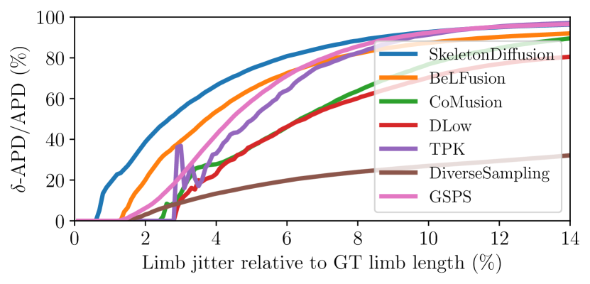
Figure 8: Diversity achieved with valid motions over total diversity according to different error tolerances on AMASS. For every method, we show the evolution of diversity ($\delta$-APD) computed with valid motions (y-axis) for which the maximal error is below a given threshold $\delta$ (x-axis). SkeletonDiffusion presents consistently the highest diversity when considering valid poses.

In the main paper we discuss our intuition on how artifacts in the generated motions may lead to increased distance between the predictions and so to a better diversity metric (APD). We wish to provide evidence of this phenomenon with an argument similar to the one employed in Fig. 7 of the main paper i.e. by inspecting the evolution of the APD metric at different tolerance thresholds of limb jitter. First, we compute the valid motions among the generated predictions per method on the AMASS dataset, discarding a sequence if it displays a bone length jitter above a given threshold $\delta$. By calculating the average pairwise distance APD only between valid motions and relating this value to the customary APD, in Fig. 8 we can see the contribution of ill-posed motions on diversity. Such evolving diversity differs significantly from the values reported in Tab. 1. Our method generates by a large margin the most diverse motions when considering realism according to limb jitter, demonstrating excellence also under strict constraints. Non-smooth curve regions display the influence of ill-posed motions on diversity when considering a small ensemble of predictions, as for CoMusion and TPK. When the number of valid motions is small and some of them present stretching, removing the unrealistic motions may considerably improve or worsen the average pairwise distance, resulting in sudden jumps in the curves. We are thus the first to demonstrate quantitatively that unrealistic motions increase diversity.

	Precision		Multimodal GT		Diversity	Realism	Body Realism
Base of $\boldsymbol{\Sigma}_{N}$							mean $\downarrow$		RMSE $\downarrow$
	ADE $\downarrow$	FDE $\downarrow$	MMADE $\downarrow$	MMFDE $\downarrow$	APD $\uparrow$	CMD $\downarrow$	str	jit	str	jit
$\mathbf{R}$	0.481	0.540	0.562	0.574	9.504	11.542	3.16	0.20	4.51	0.27
$\mathbf{R}^{hip}$	0.475	0.543	0.558	0.579	8.629	12.499	3.14	0.19	4.35	0.25
$\mathbf{A}$ (SkeletonDiffusion)	0.480	0.545	0.561	0.580	9.456	11.417	3.15	0.20	4.45	0.26

Table 8: Ablation studies for the correlation matrix $\boldsymbol{\Sigma}_{N}$ on AMASS for adjacency matrix $\mathbf{A}$, the weighted transitive closure $\mathbf{R}$, and the masked weighted transitive closure $\mathbf{R}^{hip}$.

Appendix F Further Analysis

F.1 On Nonisotropic and Isotropic Diffusion Training

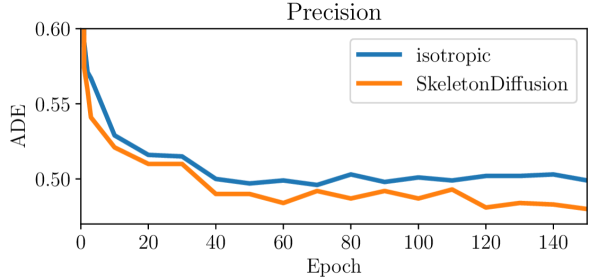
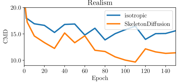
Figure 9: Our nonisotropic diffusion converges in fewer epochs than the conventional isotropic formulation.

As depicted in Fig. 9, our nonisotropic formulation converges faster than the isotropic counterparty. As the time required for a train iteration is equal among both formulations up to a few negligible matrix multiplications, our nonisotropic formulation achieves higher performance in fewer iterations. In Tab. 6, we show that for similar performance (precision ADE) our nonisotropic formulation requires fewer parameters than conventional isotropic diffusion. We report these findings as they may be relevant for HMP applications or other structured tasks employing diffusion models.

F.2 Discussion on Correlation Matrix $\boldsymbol{\Sigma}_{N}$

On the Magnitude Normalization

The magnitude of $\boldsymbol{\Sigma}_{N}$ is constrained as in Eq. 4, where, after adding entries along the diagonal, we divide by the highest eigenvalue (spectral norm). In Tab. 7, we show results on AMASS for another normalization choice, the Frobenius norm i.e. the average of the eigenvalues. While both norms deliver very similar results, we opt for the spectral norm as the realism metrics indicate lower limb stretching and joint velocity closer to the GT data (CMD). An educated guess for the subtle difference is that higher noise magnitude (Frobenius norm) eases the generation of more diverse samples (higher diversity) but at the same time loses details of fine-grained joint positions (lower realism and limb stretching).

Sophistications on the Choice of $\boldsymbol{\Sigma}_{N}$

For the correlation matrix $\boldsymbol{\Sigma}_{N}$ from Eq. 4, we opt for the most straightforward and simple starting choice, the adjacency matrix $\mathbf{A}$. Here we report further studies to two more sophisticated initial choices: the weighted transitive closure $\mathbf{R}$ and the masked weighted transitive closure $\mathbf{R}^{hip}$. Given two nodes $v_{i}$ and $v_{j}$ in the graph, the shortest path is denoted by $P(i,j)$. The number of hops between $v_{i}$ and $v_{j}$ is denoted by $h_{i,j}$. We then can express the weighted transitive closure $\mathbf{R}$ as:

$$\mathbf{R}_{i,j}:=\eta^{h_{i,j}-1}$$ (62)

with some $\eta\in(0,1)$, representing the reachability of each node weighted by the hops. As the hip joint is critical in human motion, we also consider a masked version $\mathbf{R}^{hip}$:

$$\mathbf{R}^{hip}_{i,j}=\begin{cases}\mathbf{R}_{i,j}&\text{ if }v_{hip}\in P(i,j),v_{i}\neq v_{hip},v_{j}\neq v_{hip}\\ 0&\text{ otherwise}\\ \end{cases}$$ (63)

These three node correlation matrices are visualized on the H36M dataset in Fig. 10. While all three alternatives obtain good results on AMASS in Tab. 8, we opt for the adjacency matrix $\mathbf{A}$ as it is not handcrafted and allows our nonisotropic approach to generalize in a straightforward manner to different datasets. We see the analysis of sophisticated choices for $\boldsymbol{\Sigma}_{N}$ as an exciting future direction.

Figure 10: Node correlation matrix $\boldsymbol{\Sigma}_{N}$ for different starting choices on the H36M skeleton: the adjacency matrix $\mathbf{A}$ of the skeleton graph, the weighted transitive closure $\mathbf{R}$ and the masked weighted transitive closure $\mathbf{R}^{hip}$.

F.3 Correlations of Latent Space

We visualize the skeleton latent space in terms of the correlation among different latent joint dimensions. To this end, we embed all AMASS test segments in the latent space, and compute the first principal component along the each joint dimension separately. For each embedding, we then plot the principal component of two joint dimensions against each other. In Fig. 12, we show 50 random test segments and for each 15 diffused latents. Our latent space reflects correlations connected body joints that are expected (e.g. LHip and RHip) or are less intuitive (e.g. Neck and Hip always show in the same space direction), while other joints do not exhibit univocal correlations (e.g. Wrist and Ankle of the same body side). Weak correlations (probably related to the walking pattern) can be observed between opposite joints of the lower and upper body such as RHip and LElbow.

Appendix G More Qualitative Examples

We show more qualitative results on AMASS in Figs. 13, LABEL:, 14, LABEL:, 15, LABEL:, 16, LABEL: and 17. More qualitative examples for H36M can be found in Figs. 18, LABEL:, 19, LABEL: and 20 and Fig. 11.

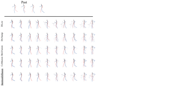
Figure 11: Qualitative Results on H36M through overlapping skeletons. Action labeled WalkTogether, segment n. 791. For each method, we display the ground truth future (thicker skeleton) overlapped by the closest prediction and the two most diverse. See Fig. 20 for a different visualization of the same qualitative.

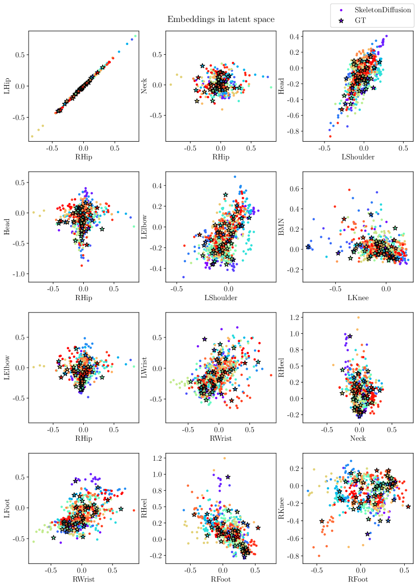
Figure 12: PCA plots of latent space embeddings for AMASS GT test segments with corresponding diffused latents generated by SkeletonDiffusion. Each GT embedding is denoted by a $\star$ of a different color, and the generated latents corresponding to the same past are denoted by a circle $\circ$ of the same color.

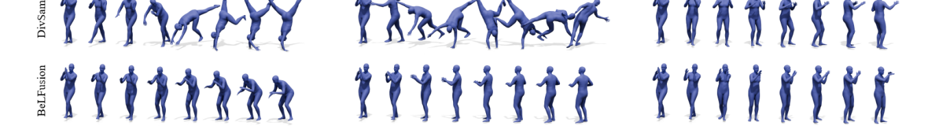
Figure 13: Qualitative Results on AMASS. From DanceDB dataset, segment n. 4122.

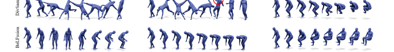
Figure 14: Qualitative Results on AMASS. From Human4D dataset, segment n. 11949.

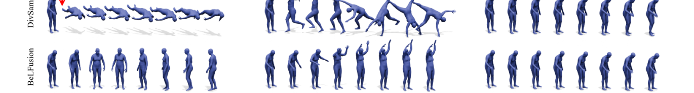
Figure 15: Qualitative Results on AMASS. From GRAB dataset, segment n. 9622.

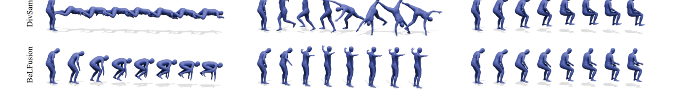
Figure 16: Qualitative Results on AMASS. From Human4D dataset, segment n. 12267.

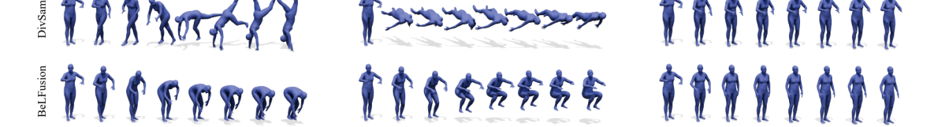
Figure 17: Qualitative Results on AMASS. From GRAB dataset, segment n. 10188.

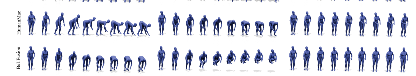
Figure 18: Qualitative Results on H36M. Action labeled WalkDog, segment n. 3122.

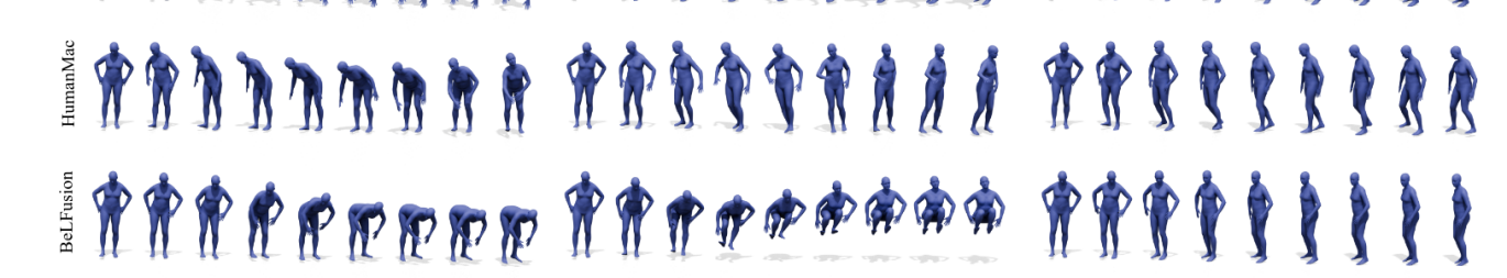
Figure 19: Qualitative Results on H36M. Action labeled Discussion, segment n. 2620.

Figure 20: Qualitative Results on H36M. Action labeled WalkTogether, segment n. 791.

References

- Adeli et al. [2021] Vida Adeli, Mahsa Ehsanpour, Ian Reid, Juan Carlos Niebles, Silvio Savarese, Ehsan Adeli, and Hamid Rezatofighi. Tripod: Human trajectory and pose dynamics forecasting in the wild. In Proceedings of the IEEE/CVF International Conference on Computer Vision, pages 13390–13400, 2021.
- Aksan et al. [2021] Emre Aksan, Manuel Kaufmann, Peng Cao, and Otmar Hilliges. A spatio-temporal transformer for 3d human motion prediction. In 2021 International Conference on 3D Vision (3DV), pages 565–574. IEEE, 2021.
- Andrist et al. [2015] Sean Andrist, Bilge Mutlu, and Adriana Tapus. Look like me: matching robot personality via gaze to increase motivation. In Proceedings of the 33rd annual ACM conference on human factors in computing systems, pages 3603–3612, 2015.
- Barquero et al. [2022] German Barquero, Johnny Núnez, Zhen Xu, Sergio Escalera, Wei-Wei Tu, Isabelle Guyon, and Cristina Palmero. Comparison of spatio-temporal models for human motion and pose forecasting in face-to-face interaction scenarios supplementary material. Proceedings of Machine Learning Research, 2022.
- Barquero et al. [2023] German Barquero, Sergio Escalera, and Cristina Palmero. Belfusion: Latent diffusion for behavior-driven human motion prediction. In Proceedings of the IEEE/CVF International Conference on Computer Vision, pages 2317–2327, 2023.
- Barsoum et al. [2017] Emad Barsoum, John Kender, and Zicheng Liu. Hpgan: Probabilistic 3d human motion prediction via gan. 2018 ieee. In CVF Conference on Computer Vision and Pattern Recognition Workshops (CVPRW), pages 1499–149909, 2017.
- Barsoum et al. [2018] Emad Barsoum, John Kender, and Zicheng Liu. Hp-gan: Probabilistic 3d human motion prediction via gan. In Proceedings of the IEEE conference on computer vision and pattern recognition workshops, pages 1418–1427, 2018.
- Bengio et al. [2009] Yoshua Bengio, Jérôme Louradour, Ronan Collobert, and Jason Weston. Curriculum learning. In Proceedings of the 26th annual international conference on machine learning, pages 41–48, 2009.
- Bhattacharyya et al. [2018] Apratim Bhattacharyya, Bernt Schiele, and Mario Fritz. Accurate and diverse sampling of sequences based on a “best of many” sample objective. In Proceedings of the IEEE Conference on Computer Vision and Pattern Recognition, pages 8485–8493, 2018.
- Brooks et al. [2024] Tim Brooks, Bill Peebles, Connor Holmes, Will DePue, Yufei Guo, Li Jing, David Schnurr, Joe Taylor, Troy Luhman, Eric Luhman, Clarence Ng, Ricky Wang, and Aditya Ramesh. Video generation models as world simulators. Page Link, 2024.
- Bütepage et al. [2017] Judith Bütepage, Hedvig Kjellström, and Danica Kragic. Anticipating many futures: Online human motion prediction and synthesis for human-robot collaboration. arXiv preprint arXiv:1702.08212, 2017.
- Cai et al. [2020] Yujun Cai, Lin Huang, Yiwei Wang, Tat-Jen Cham, Jianfei Cai, Junsong Yuan, Jun Liu, Xu Yang, Yiheng Zhu, Xiaohui Shen, et al. Learning progressive joint propagation for human motion prediction. In Computer Vision–ECCV 2020: 16th European Conference, Glasgow, UK, August 23–28, 2020, Proceedings, Part VII 16, pages 226–242. Springer, 2020.
- Cai et al. [2021] Yujun Cai, Yiwei Wang, Yiheng Zhu, Tat-Jen Cham, Jianfei Cai, Junsong Yuan, Jun Liu, Chuanxia Zheng, Sijie Yan, Henghui Ding, et al. A unified 3d human motion synthesis model via conditional variational auto-encoder. In Proceedings of the IEEE/CVF International Conference on Computer Vision, pages 11645–11655, 2021.
- Cao et al. [2020] Zhe Cao, Hang Gao, Karttikeya Mangalam, Qi-Zhi Cai, Minh Vo, and Jitendra Malik. Long-term human motion prediction with scene context. In Computer Vision–ECCV 2020: 16th European Conference, Glasgow, UK, August 23–28, 2020, Proceedings, Part I 16, pages 387–404. Springer, 2020.
- Chang et al. [2023] Pascal Chang, Jingwei Tang, Markus Gross, and Vinicius C Azevedo. How i warped your noise: a temporally-correlated noise prior for diffusion models. In The Twelfth International Conference on Learning Representations, 2023.
- Chen et al. [2023] Ling-Hao Chen, Jiawei Zhang, Yewen Li, Yiren Pang, Xiaobo Xia, and Tongliang Liu. Humanmac: Masked motion completion for human motion prediction. arXiv preprint arXiv:2302.03665, 2023.
- Cui et al. [2020] Qiongjie Cui, Huaijiang Sun, and Fei Yang. Learning dynamic relationships for 3d human motion prediction. In Proceedings of the IEEE/CVF conference on computer vision and pattern recognition, pages 6519–6527, 2020.
- Dang et al. [2021] Lingwei Dang, Yongwei Nie, Chengjiang Long, Qing Zhang, and Guiqing Li. Msr-gcn: Multi-scale residual graph convolution networks for human motion prediction. In Proceedings of the IEEE/CVF International Conference on Computer Vision, pages 11467–11476, 2021.
- Dang et al. [2022] Lingwei Dang, Yongwei Nie, Chengjiang Long, Qing Zhang, and Guiqing Li. Diverse human motion prediction via gumbel-softmax sampling from an auxiliary space. In Proceedings of the 30th ACM International Conference on Multimedia, pages 5162–5171, 2022.
- Daras et al. [2022] Giannis Daras, Mauricio Delbracio, Hossein Talebi, Alexandros G Dimakis, and Peyman Milanfar. Soft diffusion: Score matching for general corruptions. arXiv preprint arXiv:2209.05442, 2022.
- Dhariwal and Nichol [2021] Prafulla Dhariwal and Alexander Nichol. Diffusion models beat gans on image synthesis. Advances in neural information processing systems, 34:8780–8794, 2021.
- Eyring et al. [2024] Luca Eyring, Shyamgopal Karthik, Karsten Roth, Alexey Dosovitskiy, and Zeynep Akata. Reno: Enhancing one-step text-to-image models through reward-based noise optimization. arXiv preprint arXiv:2406.04312, 2024.
- Fragkiadaki et al. [2015] Katerina Fragkiadaki, Sergey Levine, Panna Felsen, and Jitendra Malik. Recurrent network models for human dynamics. In Proceedings of the IEEE international conference on computer vision, pages 4346–4354, 2015.
- Ge et al. [2023] Songwei Ge, Seungjun Nah, Guilin Liu, Tyler Poon, Andrew Tao, Bryan Catanzaro, David Jacobs, Jia-Bin Huang, Ming-Yu Liu, and Yogesh Balaji. Preserve your own correlation: A noise prior for video diffusion models. In Proceedings of the IEEE/CVF International Conference on Computer Vision, pages 22930–22941, 2023.
- Gu et al. [2024] Chunzhi Gu, Jun Yu, and Chao Zhang. Learning disentangled representations for controllable human motion prediction. Pattern Recognition, 146:109998, 2024.
- Gui et al. [2018a] Liang-Yan Gui, Yu-Xiong Wang, Xiaodan Liang, and José MF Moura. Adversarial geometry-aware human motion prediction. In Proceedings of the european conference on computer vision (ECCV), pages 786–803, 2018a.
- Gui et al. [2018b] Liang-Yan Gui, Kevin Zhang, Yu-Xiong Wang, Xiaodan Liang, José MF Moura, and Manuela Veloso. Teaching robots to predict human motion. In 2018 IEEE/RSJ International Conference on Intelligent Robots and Systems (IROS), pages 562–567. IEEE, 2018b.
- Guo et al. [2023] Wen Guo, Yuming Du, Xi Shen, Vincent Lepetit, Xavier Alameda-Pineda, and Francesc Moreno-Noguer. Back to mlp: A simple baseline for human motion prediction. In Proceedings of the IEEE/CVF Winter Conference on Applications of Computer Vision, pages 4809–4819, 2023.
- Gupta et al. [2018] Agrim Gupta, Justin Johnson, Li Fei-Fei, Silvio Savarese, and Alexandre Alahi. Social gan: Socially acceptable trajectories with generative adversarial networks. In Proceedings of the IEEE conference on computer vision and pattern recognition, pages 2255–2264, 2018.
- Gurumurthy et al. [2017] Swaminathan Gurumurthy, Ravi Kiran Sarvadevabhatla, and R Venkatesh Babu. Deligan: Generative adversarial networks for diverse and limited data. In Proceedings of the IEEE conference on computer vision and pattern recognition, pages 166–174, 2017.
- Ho et al. [2020] Jonathan Ho, Ajay Jain, and Pieter Abbeel. Denoising diffusion probabilistic models. Advances in neural information processing systems, 33:6840–6851, 2020.
- Hoogeboom and Salimans [2022] Emiel Hoogeboom and Tim Salimans. Blurring diffusion models. arXiv preprint arXiv:2209.05557, 2022.
- Huang et al. [2024] Xingchang Huang, Corentin Salaün, Cristina Vasconcelos, Christian Theobalt, Cengiz Öztireli, and Gurprit Singh. Blue noise for diffusion models. arXiv preprint arXiv:2402.04930, 2024.
- Ionescu et al. [2014] Catalin Ionescu, Dragos Papava, Vlad Olaru, and Cristian Sminchisescu. Human3.6m: Large scale datasets and predictive methods for 3d human sensing in natural environments, 2014.
- Jain et al. [2016] Ashesh Jain, Amir R Zamir, Silvio Savarese, and Ashutosh Saxena. Structural-rnn: Deep learning on spatio-temporal graphs. In Proceedings of the ieee conference on computer vision and pattern recognition, pages 5308–5317, 2016.
- Ju et al. [2023] Xuan Ju, Ailing Zeng, Jianan Wang, Qiang Xu, and Lei Zhang. Human-art: A versatile human-centric dataset bridging natural and artificial scenes. In Proceedings of the IEEE/CVF Conference on Computer Vision and Pattern Recognition, pages 618–629, 2023.
- Karunratanakul et al. [2024] Korrawe Karunratanakul, Konpat Preechakul, Emre Aksan, Thabo Beeler, Supasorn Suwajanakorn, and Siyu Tang. Optimizing diffusion noise can serve as universal motion priors. In Proceedings of the IEEE/CVF Conference on Computer Vision and Pattern Recognition, pages 1334–1345, 2024.
- Kim et al. [2022] Dongjun Kim, Byeonghu Na, Se Jung Kwon, Dongsoo Lee, Wanmo Kang, and Il-chul Moon. Maximum likelihood training of implicit nonlinear diffusion model. Advances in Neural Information Processing Systems, 35:32270–32284, 2022.
- Kipf and Welling [2016] Thomas N Kipf and Max Welling. Semi-supervised classification with graph convolutional networks. arXiv preprint arXiv:1609.02907, 2016.
- Kundu et al. [2019] Jogendra Nath Kundu, Maharshi Gor, and R Venkatesh Babu. Bihmp-gan: Bidirectional 3d human motion prediction gan. In Proceedings of the AAAI conference on artificial intelligence, pages 8553–8560, 2019.
- Lee et al. [2022] Meng-Lun Lee, Wansong Liu, Sara Behdad, Xiao Liang, and Minghui Zheng. Robot-assisted disassembly sequence planning with real-time human motion prediction. IEEE Transactions on Systems, Man, and Cybernetics: Systems, 53(1):438–450, 2022.
- Li et al. [2018] Chen Li, Zhen Zhang, Wee Sun Lee, and Gim Hee Lee. Convolutional sequence to sequence model for human dynamics. In Proceedings of the IEEE conference on computer vision and pattern recognition, pages 5226–5234, 2018.
- Li et al. [2019] Maosen Li, Siheng Chen, Xu Chen, Ya Zhang, Yanfeng Wang, and Qi Tian. Actional-structural graph convolutional networks for skeleton-based action recognition. In Proceedings of the IEEE/CVF conference on computer vision and pattern recognition, pages 3595–3603, 2019.
- Li et al. [2020] Maosen Li, Siheng Chen, Yangheng Zhao, Ya Zhang, Yanfeng Wang, and Qi Tian. Dynamic multiscale graph neural networks for 3d skeleton based human motion prediction. In Proceedings of the IEEE/CVF conference on computer vision and pattern recognition, pages 214–223, 2020.
- Liu et al. [2023] Shuijing Liu, Peixin Chang, Zhe Huang, Neeloy Chakraborty, Kaiwen Hong, Weihang Liang, D Livingston McPherson, Junyi Geng, and Katherine Driggs-Campbell. Intention aware robot crowd navigation with attention-based interaction graph. In 2023 IEEE International Conference on Robotics and Automation (ICRA), pages 12015–12021. IEEE, 2023.
- Liu et al. [2019] Zhenguang Liu, Shuang Wu, Shuyuan Jin, Qi Liu, Shijian Lu, Roger Zimmermann, and Li Cheng. Towards natural and accurate future motion prediction of humans and animals. In Proceedings of the IEEE/CVF Conference on Computer Vision and Pattern Recognition, pages 10004–10012, 2019.
- Liu et al. [2021] Zhenguang Liu, Kedi Lyu, Shuang Wu, Haipeng Chen, Yanbin Hao, and Shouling Ji. Aggregated multi-gans for controlled 3d human motion prediction. In Proceedings of the AAAI conference on artificial intelligence, pages 2225–2232, 2021.
- Luo [2022] Calvin Luo. Understanding diffusion models: A unified perspective. arXiv preprint arXiv:2208.11970, 2022.
- Lyu et al. [2022a] Kedi Lyu, Haipeng Chen, Zhenguang Liu, Beiqi Zhang, and Ruili Wang. 3d human motion prediction: A survey. Neurocomputing, 489:345–365, 2022a.
- Lyu et al. [2022b] Zhaoyang Lyu, Xudong Xu, Ceyuan Yang, Dahua Lin, and Bo Dai. Accelerating diffusion models via early stop of the diffusion process. arXiv preprint arXiv:2205.12524, 2022b.
- Ma et al. [2022] Tiezheng Ma, Yongwei Nie, Chengjiang Long, Qing Zhang, and Guiqing Li. Progressively generating better initial guesses towards next stages for high-quality human motion prediction. In Proceedings of the IEEE/CVF Conference on Computer Vision and Pattern Recognition, pages 6437–6446, 2022.
- Mahmood et al. [2019] Naureen Mahmood, Nima Ghorbani, Nikolaus F Troje, Gerard Pons-Moll, and Michael J Black. Amass: Archive of motion capture as surface shapes. In Proceedings of the IEEE/CVF international conference on computer vision, pages 5442–5451, 2019.
- Mao et al. [2020] Wei Mao, Miaomiao Liu, and Mathieu Salzmann. History repeats itself: Human motion prediction via motion attention. In Computer Vision–ECCV 2020: 16th European Conference, Glasgow, UK, August 23–28, 2020, Proceedings, Part XIV 16, pages 474–489. Springer, 2020.
- Mao et al. [2021] Wei Mao, Miaomiao Liu, and Mathieu Salzmann. Generating smooth pose sequences for diverse human motion prediction. In Proceedings of the IEEE/CVF International Conference on Computer Vision, pages 13309–13318, 2021.
- Martinez et al. [2017] Julieta Martinez, Michael J Black, and Javier Romero. On human motion prediction using recurrent neural networks. In Proceedings of the IEEE conference on computer vision and pattern recognition, pages 2891–2900, 2017.
- Martínez-González et al. [2021] Angel Martínez-González, Michael Villamizar, and Jean-Marc Odobez. Pose transformers (potr): Human motion prediction with non-autoregressive transformers. In Proceedings of the IEEE/CVF International Conference on Computer Vision, pages 2276–2284, 2021.
- Medjaouri and Desai [2022] Omar Medjaouri and Kevin Desai. Hr-stan: High-resolution spatio-temporal attention network for 3d human motion prediction. In Proceedings of the IEEE/CVF Conference on Computer Vision and Pattern Recognition, pages 2540–2549, 2022.
- Nichol and Dhariwal [2021] Alexander Quinn Nichol and Prafulla Dhariwal. Improved denoising diffusion probabilistic models. In International Conference on Machine Learning, pages 8162–8171. PMLR, 2021.
- Paden et al. [2016] Brian Paden, Michal Čáp, Sze Zheng Yong, Dmitry Yershov, and Emilio Frazzoli. A survey of motion planning and control techniques for self-driving urban vehicles. IEEE Transactions on intelligent vehicles, 1(1):33–55, 2016.
- Pavllo et al. [2018] Dario Pavllo, David Grangier, and Michael Auli. Quaternet: A quaternion-based recurrent model for human motion. arXiv preprint arXiv:1805.06485, 2018.
- Ramesh et al. [2022] Aditya Ramesh, Prafulla Dhariwal, Alex Nichol, Casey Chu, and Mark Chen. Hierarchical text-conditional image generation with clip latents. arXiv preprint arXiv:2204.06125, 1(2):3, 2022.
- Rombach et al. [2022] Robin Rombach, Andreas Blattmann, Dominik Lorenz, Patrick Esser, and Björn Ommer. High-resolution image synthesis with latent diffusion models, 2022.
- Rudenko et al. [2020] Andrey Rudenko, Luigi Palmieri, Michael Herman, Kris M Kitani, Dariu M Gavrila, and Kai O Arras. Human motion trajectory prediction: A survey. The International Journal of Robotics Research, 39(8):895–935, 2020.
- Saadatnejad et al. [2023] Saeed Saadatnejad, Ali Rasekh, Mohammadreza Mofayezi, Yasamin Medghalchi, Sara Rajabzadeh, Taylor Mordan, and Alexandre Alahi. A generic diffusion-based approach for 3d human pose prediction in the wild, 2023.
- Salzmann et al. [2022] Tim Salzmann, Marco Pavone, and Markus Ryll. Motron: Multimodal probabilistic human motion forecasting. In Proceedings of the IEEE/CVF Conference on Computer Vision and Pattern Recognition, pages 6457–6466, 2022.
- Stevens et al. [2023] Tristan SW Stevens, Hans van Gorp, Faik C Meral, Junseob Shin, Jason Yu, Jean-Luc Robert, and Ruud JG van Sloun. Removing structured noise with diffusion models. arXiv preprint arXiv:2302.05290, 2023.
- Sun and Chowdhary [2024] Jiarui Sun and Girish Chowdhary. Comusion: Towards consistent stochastic human motion prediction via motion diffusion–supplementary material–. European Conference on Computer Vision, 2024.
- Taylor et al. [2020] William Taylor, Syed Aziz Shah, Kia Dashtipour, Adnan Zahid, Qammer H Abbasi, and Muhammad Ali Imran. An intelligent non-invasive real-time human activity recognition system for next-generation healthcare. Sensors, 20(9):2653, 2020.
- Teramae et al. [2017] Tatsuya Teramae, Tomoyuki Noda, and Jun Morimoto. Emg-based model predictive control for physical human–robot interaction: Application for assist-as-needed control. IEEE Robotics and Automation Letters, 3(1):210–217, 2017.
- Troje [2002] Nikolaus F Troje. Decomposing biological motion: A framework for analysis and synthesis of human gait patterns. Journal of vision, 2(5):2–2, 2002.
- Vahdat et al. [2021] Arash Vahdat, Karsten Kreis, and Jan Kautz. Score-based generative modeling in latent space. 2021. arXiv preprint arXiv:2106.05931, 2021.
- Van Welbergen et al. [2010] Herwin Van Welbergen, Ben JH Van Basten, Arjan Egges, Zs M Ruttkay, and Mark H Overmars. Real time animation of virtual humans: a trade-off between naturalness and control. In Computer Graphics Forum, pages 2530–2554. Wiley Online Library, 2010.
- Vaswani et al. [2017] Ashish Vaswani, Noam Shazeer, Niki Parmar, Jakob Uszkoreit, Llion Jones, Aidan N Gomez, Łukasz Kaiser, and Illia Polosukhin. Attention is all you need. Advances in neural information processing systems, 30, 2017.
- Veličković et al. [2017] Petar Veličković, Guillem Cucurull, Arantxa Casanova, Adriana Romero, Pietro Lio, and Yoshua Bengio. Graph attention networks. arXiv preprint arXiv:1710.10903, 2017.
- Voleti et al. [2022] Vikram Voleti, Christopher Pal, and Adam Oberman. Score-based denoising diffusion with non-isotropic gaussian noise models. NeurIPS 2022 Workshop on Score-Based Methods, 2022.
- von Marcard et al. [2018] Timo von Marcard, Roberto Henschel, Michael Black, Bodo Rosenhahn, and Gerard Pons-Moll. Recovering accurate 3d human pose in the wild using imus and a moving camera. In European Conference on Computer Vision (ECCV), 2018.
- Walker et al. [2017] Jacob Walker, Kenneth Marino, Abhinav Gupta, and Martial Hebert. The pose knows: Video forecasting by generating pose futures. In Proceedings of the IEEE international conference on computer vision, pages 3332–3341, 2017.
- Wang et al. [2021] Chenxi Wang, Yunfeng Wang, Zixuan Huang, and Zhiwen Chen. Simple baseline for single human motion forecasting. In Proceedings of the IEEE/CVF International Conference on Computer Vision, pages 2260–2265, 2021.
- Wang et al. [2023] Jiong Wang, Fengyu Yang, Wenbo Gou, Bingliang Li, Danqi Yan, Ailing Zeng, Yijun Gao, Junle Wang, and Ruimao Zhang. Freeman: Towards benchmarking 3d human pose estimation in the wild, 2023.
- Wei et al. [2023] Dong Wei, Huaijiang Sun, Bin Li, Jianfeng Lu, Weiqing Li, Xiaoning Sun, and Shengxiang Hu. Human joint kinematics diffusion-refinement for stochastic motion prediction. In Proceedings of the AAAI Conference on Artificial Intelligence, pages 6110–6118, 2023.
- Xu et al. [2024] Guowei Xu, Jiale Tao, Wen Li, and Lixin Duan. Learning semantic latent directions for accurate and controllable human motion prediction. European Conference on Computer Vision, 2024.
- Xu et al. [2022] Sirui Xu, Yu-Xiong Wang, and Liang-Yan Gui. Diverse human motion prediction guided by multi-level spatial-temporal anchors. In European Conference on Computer Vision, pages 251–269. Springer, 2022.
- Xu et al. [2023a] Sirui Xu, Zhengyuan Li, Yu-Xiong Wang, and Liang-Yan Gui. Interdiff: Generating 3d human-object interactions with physics-informed diffusion. In Proceedings of the IEEE/CVF International Conference on Computer Vision, pages 14928–14940, 2023a.
- Xu et al. [2023b] Sirui Xu, Yu-Xiong Wang, and Liangyan Gui. Stochastic multi-person 3d motion forecasting. In The Eleventh International Conference on Learning Representations, 2023b.
- Yan et al. [2018] Xinchen Yan, Akash Rastogi, Ruben Villegas, Kalyan Sunkavalli, Eli Shechtman, Sunil Hadap, Ersin Yumer, and Honglak Lee. Mt-vae: Learning motion transformations to generate multimodal human dynamics. In Proceedings of the European conference on computer vision (ECCV), pages 265–281, 2018.
- Yang et al. [2023] Jie Yang, Ailing Zeng, Feng Li, Shilong Liu, Ruimao Zhang, and Lei Zhang. Neural interactive keypoint detection. In Proceedings of the IEEE/CVF International Conference on Computer Vision, pages 15122–15132, 2023.
- Yuan and Kitani [2019] Ye Yuan and Kris Kitani. Diverse trajectory forecasting with determinantal point processes. arXiv preprint arXiv:1907.04967, 2019.
- Yuan and Kitani [2020] Ye Yuan and Kris Kitani. Dlow: Diversifying latent flows for diverse human motion prediction. In Computer Vision–ECCV 2020: 16th European Conference, Glasgow, UK, August 23–28, 2020, Proceedings, Part IX 16, pages 346–364. Springer, 2020.
- Zhang and Sennrich [2019] Biao Zhang and Rico Sennrich. Root mean square layer normalization. Advances in Neural Information Processing Systems, 32, 2019.
- Zhang et al. [2021] Yan Zhang, Michael J Black, and Siyu Tang. We are more than our joints: Predicting how 3d bodies move. In Proceedings of the IEEE/CVF Conference on Computer Vision and Pattern Recognition, pages 3372–3382, 2021.
- Zheng et al. [2022] Huangjie Zheng, Pengcheng He, Weizhu Chen, and Mingyuan Zhou. Truncated diffusion probabilistic models and diffusion-based adversarial auto-encoders. arXiv preprint arXiv:2202.09671, 2022.