The all-charm tetraquark and its contribution
to two-photon processes

Abstract

Prompted by several potential tetraquark states that have been reported by the LHCb, CMS and ATLAS collaborations in the di-$J/\Psi$ and $J/\Psi\Psi(2S)$ spectra, we investigate their contribution to two-photon processes. Within a non-relativistic potential model for the all-charm tetraquark states, we calculate the two-photon decay widths of these states, and test model independent sum rule predictions. Imposing such sum rule constraints allows us to predict the light-by-light scattering cross sections in a consistent way and check if any excess, in comparison to the Standard Model prediction, as reported by ongoing ATLAS experiments can be attributed to intermediate exotic states.

I Introduction

In recent years, a plethora of potential tetraquark states have been uncovered by several experiments. They can be composed of only light quarks, heavy quarks or a mixture of both. A candidate of the second category is the all-charm tetraquark, which is a $cc\overline{c}\overline{c}$ bound state. The first indication of an all-charm tetraquark state was discovered by the LHCb Collaboration as a resonance around $6.9\text{\,}\mathrm{GeV}$, $X(6900)$ in the di-$J/\Psi$ invariant mass spectrum [1]. Shortly afterwards, the ATLAS collaboration confirmed the excess observed in the LHCb analysis and described the data using a three resonance model [2]. Simultaneously, the CMS collaboration also confirmed the excess [3] and employed a three resonance description of the observed structure, including three Breit-Wigner resonances and their interferences. The resulting resonances and their corresponding widths are shown in Table 1.

Table 1: Breit-Wigner resonance masses and widths of $cc\overline{c}\overline{c}$ states seen in di-$J/\Psi$ spectrum with interference from Ref. [3]

resonance $i$	$M_{i}($\text{\,}\mathrm{GeV}$)$	$\Gamma_{i}($\text{\,}\mathrm{GeV}$)$
$1$	$6.638^{+0.043+0.016}_{-0.038-0.031}$	$0.440^{+0.230+0.110}_{-0.200-0.240}$
$2$	$6.847^{+0.044+0.048}_{-0.028-0.020}$	$0.191^{+0.066+0.025}_{-0.049-0.017}$
$3$	$7.134^{+0.048+0.041}_{-0.025-0.015}$	$0.097^{+0.040+0.029}_{-0.029-0.026}$

In parallel to this, in 2017 the ATLAS Collaboration found the first evidence of Light-by-Light (LbL) scattering [4] in heavy-ion collisions. Subsequently, in a more recent analysis [5] of the entire data coming from Run 2 at the LHC, this discovery was strengthened to reach a significance of $8.2\ \sigma$. The resulting data in the di-photon electroproduction cross section has indicated a potential discrepancy with the Standard Model predicted value, especially in the $5$ to $10\text{\,}\mathrm{GeV}$ region.

On the theoretical side, exotic multiquark states have been discussed for decades. The first work on an all-charm tetraquark configuration was made in Refs. [6, 7, 8]. Since then, many approaches have been used to predict the mass spectra for the resulting states. One of the main ways to tackle this problem is the diquark picture for the quark interactions inside the bound state. In combination with a potential, such as the Cornell potential [9] it can be used to predict the bound states and their characteristics.

LbL scattering, on the other hand, is one of the earliest processes predicted by QED [10, *Heisenberg_1936]. Model-independent sum rules for LbL processes [12] are particularly useful in this context. Additionally, work performed in [13] bridges the all-charm tetraquark searches with the LbL studies. In particular, it suggests that an all-charm tetraquark candidate, in this case the $X(6900)$ could be responsible for the excess of LbL events seen by the ATLAS Collaboration.

In this work, we follow and expand upon the diquark potential model description of Ref. [14] to calculate the predicted all-charm tetraquark spectrum, including the $D$-states as well. For the resulting states we then calculate the two-photon production widths, for the first time. Our aim is to check whether these states allow to explain the perceived experimental excess in LbL data. Putting these results against model-independent sum rule for real photons we propose a modified potential model for these states that can potentially accommodate for the existing experimental data.

In Section II we describe the diquark potential model used in this work and calculate the resulting spectrum. After that, in Section III we first calculate the perturbative two-photon widths for axial-vector diquarks and use them to predict the widths of the all-charm tetraquark bound states. In Section IV, we introduce the modified potential model which is fitted to the experimental potential all-charm tetraquark states and is then compared with other works. Finally, Section V consists of the main conclusions and an outlook.

II Tetraquark Potential Model

Considering all interactions between four valence quarks in a tetraquark requires solving a complicated four-body problem. A common approximation is therefore to introduce a diquark picture. In such framework, two quarks are bound to form a diquark quasi-particle, and antiquarks form the antidiquark respectively. Two of those composite particles are treated as compact and an attractive interaction between them gives rise to the bound tetraquark state. Consequently, in such picture the complicated four-body problem is reduced to three two-body ones. A pictorial representation of this concept is shown in Figure 1.

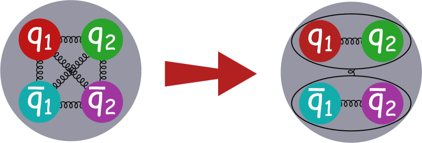
Figure 1: Schematic representation of the diquark picture considering one-gluon interactions. In this framework, the four-body problem (left) is converted to three simpler two-body problems with one-gluon interactions (right). The quarks $q_{1}$, $q_{2}$ form the diquark and $\overline{q}_{1}$, $\overline{q}_{2}$ form the antidiquark.

The color content of an all-charm tetraquark configuration follow from the $SU(3)_{c}$ representations. Two quarks, described by a color triplet representation, are combined as

$$\mathbf{3}\otimes\mathbf{3}=\mathbf{6}\oplus\mathbf{\overline{3}}.$$ (1)

The sextet configuration is repulsive, while the anti-triplet is attractive. For this analysis, only the attractive anti-triplet will be considered. Similarly, antiquarks couple as,

$$\mathbf{\overline{3}}\otimes\mathbf{\overline{3}}=\mathbf{\overline{6}}\oplus\mathbf{3},$$ (2)

likewise only the triplet will be used. The diquark anti-triplet and the antidiquark triplet are then combined as,

$$\mathbf{3}\otimes\mathbf{\overline{3}}=\mathbf{8}\oplus\mathbf{1}.$$ (3)

We will only consider resulting color singlet tetraquark bound states, in Eq. (3), which is the most attractive configuration under one-gluon exchange.

Due to the relatively large mass of the charm quark, a non-relativistic framework will be adopted. Consequently, for each of the three two-body problems, we will solve the reduced Schrödinger equation, which is

$$\left[\frac{1}{2m}\left(-\frac{\text{d}^{2}}{\text{d}r^{2}}+\frac{l(l+1)}{r^{2}}\right)+\mathcal{V}(r)\right]u(r)=Eu(r),$$ (4)

where $u(r)$ corresponds to the reduced wavefunction,

$$u(r)=\frac{R(r)}{r}.$$ (5)

The interaction between the charm quarks and between the charmed diquarks is then approximated by a potential of the Cornell type [15], consisting of central potential, complemented by spin-spin, spin-orbit and tensor terms. The considered potential given by [14],

$$V= \mathcal{V}_{C}(r)+\mathcal{V}_{SS}(r)\delta^{3}(\mathbf{r})\mathbf{S}_{1}\cdot\mathbf{S}_{2}+\mathcal{V}_{LS}(r)\mathbf{L\cdot S}$$ (6)

$$+\mathcal{V}_{T}(r)\biggl{(}\frac{(\mathbf{S}_{1}\cdot\mathbf{r})(\mathbf{S}_{2}\cdot\mathbf{r})}{r^{2}}-\frac{1}{3}\mathbf{S}_{1}\cdot\mathbf{S}_{2}\biggr{)},$$

with

$$\mathcal{V}_{C}(r)= \kappa_{s}\frac{\alpha_{s}}{r}+br,$$ (7)

$$\mathcal{V}_{SS}(r)= -\frac{8\kappa_{s}\alpha_{s}\pi}{3m^{2}},$$

$$\mathcal{V}_{LS}(r)= -\frac{3\kappa_{s}\alpha_{s}}{2m^{2}}\frac{1}{r^{3}}-\frac{b}{2m^{2}}\frac{1}{r},$$

$$\mathcal{V}_{T}(r)= -\frac{12\kappa_{s}\alpha_{s}}{4m^{2}}\frac{1}{r^{3}},$$

where $r$ corresponds to the radius from the interaction center. Eq. (LABEL:eq:potential_specific) contains four parameters, $\kappa_{s}$ is the color factor resulting from the one-gluon exchange potential, $\alpha_{s}$ is the strong coupling constant, $b$ is the slope parameter from the confinement potential and $m$ is the mass of the constituents (quarks or diquarks and their anti-particles).

The Cornell potential requires a numerical solution for the reduced Schrödinger equation. To avoid the singular $\delta$-function in the spin-spin interaction potential, a Gaussian smearing function is commonly used instead. Introducing a smearing parameter $\sigma$, the spin-spin interaction becomes,

$$V_{SS}=\mathcal{V}_{SS}(r)\left(\frac{\sigma}{\sqrt{\pi}}\right)^{3}e^{-\sigma^{2}r^{2}}\mathbf{S_{1}\cdot S_{2}}.$$ (8)

The color factor $\kappa_{s}$ depends on the color configuration and can be calculated from tree-level Feynman graphs. In Table 2 we have listed the factor $\kappa_{s}$ for a quark-quark anti-triplet (same for antiquark-antiquark triplet) configuration and a diquark-antidiquark singlet.

Table 2: Table of color factors $\kappa_{s}$ for the different configurations considered.

configuration	$\kappa_{s}$
singlet	$-4/3$
anti-triplet	$-2/3$

As the color triplet state of a diquark composed of two charm quarks is anti-symmetric, its spatial-spin wavefunction has to be symmetric to comply with the Pauli principle. This leads for ground state diquarks (in an s-wave orbital state) to a symmetric spin-1 configuration. As a result, the ground state $cc$ or $\overline{c}\overline{c}$ states are spin-$1$ axial-vector diquark states. Subsequently, the diquark and antidiquark spins combine to give three different tetraquark configurations, corresponding with total spin $S=0,1,2$. The total spin $S$ combines with the relative angular momentum between diquark and anti-diquark to give the total tetraquark angular momentum $J$. When the angular momenta operators act upon wavefunctions of tetraquark states with definite quantum numbers, they generate the following expectation values for the operators of $V_{SS}$ and $V_{LS}$,

$$\langle\mathbf{S}_{1}\cdot\mathbf{S}_{2}\rangle=\frac{1}{2}\{S(S+1))-S_{1}(S_{1}+1)-S_{2}(S_{2}+1)\},$$

and

$$\langle\mathbf{S\cdot L}\rangle=\frac{1}{2}\{J(J+1)-L(L+1)-S(S+1)\}.$$

On the other hand, the tensor operator of $V_{T}$ is more involved. Our approach and notation is based on Ref. [14]. The tensor operator for the tetraquark is defined as

$$\mathbf{T}_{d\overline{d}}=12\left(\frac{(\mathbf{S}_{d}\cdot\mathbf{r})(\mathbf{S}_{\overline{d}}\cdot\mathbf{r})}{r^{2}}-\frac{1}{3}\mathbf{S}_{d}\cdot\mathbf{S}_{\overline{d}}\right).$$ (9)

Eq. (9) can be expressed as rank-2 tensors that independently act on each diquark as follows:

$$\mathbf{T}_{d\overline{d}}=4\left(T_{0}+T^{\prime}_{0}+T_{1}+T_{-1}+T_{2}+T_{-2}\right),$$ (10)

with

$$T_{0} =2\sqrt{\frac{4\pi}{5}}Y^{0}_{2}(\theta,\phi)S_{dz}S_{\overline{d}z}$$ (11)

$$T^{\prime}_{0} =-\frac{1}{4}2\sqrt{\frac{4\pi}{5}}Y^{0}_{2}(\theta,\phi)(S_{d+}S_{\overline{d}-}+S_{d-}S_{\overline{d}+}),$$

$$T_{1} =\frac{3}{2}\sqrt{\frac{8\pi}{15}}Y^{-1}_{2}(\theta,\phi)(S_{dz}S_{\overline{d}+}+S_{d+}S_{\overline{d}z}),$$

$$T_{-1} =-\frac{3}{2}\sqrt{\frac{8\pi}{15}}Y^{1}_{2}(\theta,\phi)(S_{dz}S_{\overline{d}-}+S_{d-}S_{\overline{d}z}),$$

$$T_{2} =3\sqrt{\frac{2\pi}{15}}Y^{-2}_{2}(\theta,\phi)S_{d+}S_{\overline{d}+},$$

$$T_{-2} =3\sqrt{\frac{2\pi}{15}}Y^{2}_{2}(\theta,\phi)S_{d-}S_{\overline{d}-},$$

where $S_{d(\overline{d})z},\ S_{d(\overline{d})z+}$ and $S_{d(\overline{d})z-}$ correspond to the $z$-component, the creation and annihilation operators diquark (antidiquark) in the tetraquark construction and $Y^{m_{L}}_{L}(\theta,\phi)$ refers to the spherical harmonics. The only remaining point is to decompose the tetraquark states into diquark spin eigenstates.

States with $L=0$ force the tensor factor to be trivially zero. For $L=1$ the factors were calculated in Ref [14]. We extend their calculation for $L=2$, for which the tensor factors are presented in Table 3. An example case of this calculation is provided in Appendix A.

Table 3: Tensor factor $\langle T_{d\overline{d}}\rangle$ results for tetraquark states states with $L=2$.

$(L,S,J)$	$\langle T_{d\overline{d}}\rangle$
$(2,0,2)$	$0$
$(2,1,1)$	$-104/35$
$(2,1,2)$	$12/7$
$(2,1,3)$	$-8/7$
$(2,2,0)$	$-28/5$
$(2,2,1)$	$-68/35$
$(2,2,2)$	$132/49$
$(2,2,3)$	$32/7$
$(2,2,4)$	$-16/7$

The next step is to solve the Schrödinger equation numerically for the potential of Eq. (6). Due to their small relative contribution compared to the central part of the potential, we can treat $V_{LS}$ and $V_{T}$ as perturbations. As a first approach of producing the all-charm tetraquark spectrum the same parameters as in Ref [14] were used:

$$\begin{gathered}\alpha_{s}=0.5202,\\ m_{d}=$3.1334\text{\,}\mathrm{GeV}$,\\ b=$0.1463\text{\,}{\mathrm{GeV}}^{2}$,\\ \sigma=$1.0831\text{\,}\mathrm{GeV}$.\end{gathered}$$ (12)

Table 4: All-charm tetraquark bound state potential contributions with $1^{3}S_{1}$ diquarks for states with $L=2$. The same parameters and the same number of digits were used as in [14].

$N^{2S+1}{L}_{J}$	$E_{d\overline{d}}\ ($\text{\,}\mathrm{GeV}$)$	$\langle T\rangle\ ($\text{\,}\mathrm{GeV}$)$	$\langle V_{V}\rangle\ ($\text{\,}\mathrm{GeV}$)$	$\langle V_{b}\rangle\ ($\text{\,}\mathrm{GeV}$)$	$\langle V_{SS}\rangle\ ($\text{\,}\mathrm{GeV}$)$	$\langle V_{LS}\rangle\ ($\text{\,}\mathrm{GeV}$)$	$\langle V_{T}\rangle\ ($\text{\,}\mathrm{GeV}$)$
$1^{1}D_{2}$	$0.5809$	$0.3591$	$-0.2424$	$0.4662$	$-0.0020$	$0$	$0$
$1^{3}D_{1}$	$0.5819$	$0.3568$	$-0.2415$	$0.4675$	$-0.0009$	$-0.0126$	$-0.0034$
$1^{3}D_{2}$	$0.5819$	$0.3568$	$-0.2415$	$0.4675$	$-0.0009$	$-0.0042$	$0.0019$
$1^{3}D_{3}$	$0.5819$	$0.3568$	$-0.2415$	$0.4675$	$-0.0009$	$0.0084$	$-0.0013$
$1^{5}D_{0}$	$0.5837$	$0.3526$	$-0.2398$	$0.4700$	$0.0009$	$-0.0239$	$-0.0061$
$1^{5}D_{1}$	$0.5837$	$0.3526$	$-0.2398$	$0.4700$	$0.0009$	$-0.0200$	$-0.0021$
$1^{5}D_{2}$	$0.5837$	$0.3526$	$-0.2398$	$0.4700$	$0.0009$	$-0.0120$	$0.0029$
$1^{5}D_{3}$	$0.5837$	$0.3526$	$-0.2398$	$0.4700$	$0.0009$	$0$	$0.0050$
$1^{5}D_{4}$	$0.5837$	$0.3526$	$-0.2398$	$0.4700$	$0.0009$	$0.0160$	$-0.0025$

The method employed to solve Eq. (4) was spatial democratization with the Arnoldi iteration [16]. The solution range was $$0\text{\,}{\mathrm{GeV}}^{-1}$\leq r\leq$40\text{\,}{\mathrm{GeV}}^{-1}$$ covered with a step of $0.001\text{\,}{\mathrm{GeV}}^{-1}$ and the radial wavefunction $R(r)$ was normalized to unity. The masses of the all-charm tetraquark states were computed by,

$$M_{T}({}^{2S+1}{L}_{J})= 2m_{d}+E_{d\overline{d}}$$ (13)

$$+\langle V_{LS}(r)+V_{T}(r)\rangle_{d\overline{d}},$$

where $E_{d\overline{d}}$ is the energy eigenvalue of the diquark-antidiquark system. The subscript $d\overline{d}$ states that the expectation value calculation used the diquark eigenfunctions.

Since the problem has already been solved for $S$ and $P$-states in Ref. [14] which we reproduced as a check, we are focusing here on the $D$-states of the spectrum. The potential contributions for $L=2$ are presented in Table 4 for the first energy shell. As for notation, $V_{b}$ corresponds to the linear confinement term, $T$ is the kinetic energy of the bound states and $V_{V}$ is the Coulomb term of Eq. (LABEL:eq:potential_specific). Contributions for $V_{LS}$ and $V_{T}$ are significantly smaller than $E_{d\overline{d}}$, thus justifying the assumption made above. The masses of the all-charm tetraquark bound $D$-states are presented in Table 5 for the first four energy levels. In each shell there are multiple states in a relatively small energy region making the experimental distinction between them potentially difficult. The numerical solutions also yield the interpolated radial wavefunction $R(r)$ and its value at origin which along with the mass of the tetraquark states enter the further calculations of two-photon production.

Table 5: All-charm tetraquark masses with $1^{3}S_{1}$ diquarks for states with $L=2$. The same parameters and the same number of digits were used as in Ref [14].

	$M_{T}\ ($\text{\,}\mathrm{GeV}$)$
${}^{2S+1}{L}_{J}$	$N=1$	$N=2$	$N=3$	$N=4$
${}^{1}D_{2}$	$6.8477$	$7.1460$	$7.4040$	$7.6365$
${}^{3}D_{1}$	$6.8328$	$7.1318$	$7.3900$	$7.6227$
${}^{3}D_{2}$	$6.8464$	$7.1450$	$7.4030$	$7.6356$
${}^{3}D_{3}$	$6.8558$	$7.1545$	$7.4127$	$7.6453$
${}^{5}D_{0}$	$6.8204$	$7.1208$	$7.3795$	$7.6125$
${}^{5}D_{1}$	$6.8284$	$7.1284$	$7.3869$	$7.6197$
${}^{5}D_{2}$	$6.8415$	$7.1409$	$7.3992$	$7.6318$
${}^{5}D_{3}$	$6.8555$	$7.1545$	$7.4127$	$7.6453$
${}^{5}D_{4}$	$6.8640$	$7.1633$	$7.4218$	$7.6547$

III Two-photon production of tetraquarks

Using the tetraquark wavefunctions as bound states of a diquark-antidiquark, we are now in a position to calculate the production rate for a tetraquark bound state in the fusion of two photons, or equivalently the decay rate of the state to two photons. The resulting Feynman diagrams for computing the latter process are presented in Figure 2. Two photons annihilate to produce diquarks (double line) which form the all-charm tetraquark state with quantum numbers $J^{PC}$. The photon to diquark process can be calculated with perturbative methods. The blob indicates the tetraquark wavefunction, obtained as diquark-antidiquark bound state.

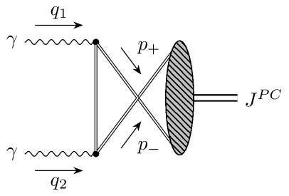
(a)

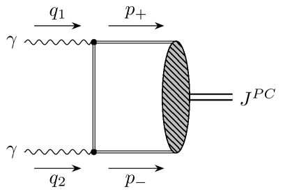
(b)

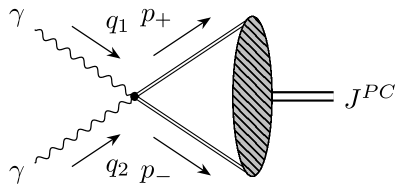
(c)

Figure 2: Feynman graphs for the two photon to two diquark process with the production of $J^{PC}$ tetraquark state.

To describe the vertex for spin-$1$ diquarks interacting with photons a natural choice is the Standard Model $W$-boson coupling, which yields cross sections that respect tree-level unitarity. The specific Feynman rules can be found in Appendix B. We work in the center-of-mass frame with the kinematics and the momenta assignments presented in Figure 3, with $p_{+},\ p_{-}$ corresponding to the (anti)diquark four-momenta, $q_{1},\ q_{2}$ to the photon four-momenta and where $\theta$ is the angle between $\mathbf{q}_{1}$ with $\mathbf{p}_{-}$.

Figure 3: Feynman graphs for the two photon to two diquark process with the production of $J^{PC}$ tetraquark state.

In order to simplify the process, we use the helicity amplitude method. We refer for the details of the calculation to Appendix B, which yields the helicity amplitudes

$$\mathcal{M}_{\lambda_{+},\lambda_{-}}^{\lambda_{1},\lambda_{2}}=\varepsilon_{\nu}(q_{2},\lambda_{2})\varepsilon_{\mu}(q_{1},\lambda_{1})\varepsilon_{\alpha}^{*}(p_{+},\lambda_{+})\varepsilon_{\beta}^{*}(p_{-},\lambda_{-})\left[\mathcal{M}^{\alpha\beta,\mu\nu}_{a}+\mathcal{M}^{\alpha\beta,\mu\nu}_{b}+\mathcal{M}^{\alpha\beta,\mu\nu}_{c}\right],$$ (14)

where

$$\mathcal{M}^{\alpha\beta,\mu\nu}_{a} =\frac{2ie_{d}^{2}}{q_{1}\cdot p_{-}}\biggl{[}g^{\alpha\beta}p_{-}^{\mu}p_{+}^{\nu}+g^{\mu\nu}q_{1}^{\beta}q_{2}^{\alpha}+g^{\alpha\nu}(-q_{2}^{\mu}q_{1}^{\beta}-p_{-}^{\mu}q_{2}^{\beta})+g^{\beta\mu}(-q_{1}^{\nu}q_{2}^{\alpha}-p_{+}^{\nu}q_{1}^{\alpha})$$ (15)

$$\qquad+g^{\alpha\mu}p_{+}^{\nu}q_{1}^{\beta}+g^{\beta\nu}p_{-}^{\mu}q_{2}^{\alpha}+g^{\alpha\nu}g^{\beta\mu}\biggl{(}-\frac{1}{2}q_{1}\cdot p_{-}+q_{1}\cdot q_{2}\biggr{)}\biggr{]},$$

$$\mathcal{M}^{\alpha\beta,\mu\nu}_{b} =\frac{2ie_{d}^{2}}{q_{1}\cdot p_{-}}\biggl{[}g^{\alpha\beta}p_{+}^{\mu}p_{-}^{\nu}+g^{\mu\nu}q_{2}^{\beta}q_{1}^{\alpha}+g^{\alpha\mu}(-q_{2}^{\beta}q_{1}^{\nu}-p_{-}^{\nu}q_{1}^{\beta})+g^{\beta\nu}(-q_{2}^{\mu}q_{1}^{\alpha}-p_{+}^{\mu}q_{2}^{\alpha})$$

$$\qquad+g^{\alpha\nu}p_{+}^{\mu}q_{2}^{\beta}+g^{\beta\mu}p_{-}^{\nu}q_{1}^{\alpha}+g^{\alpha\mu}g^{\beta\nu}\biggl{(}-\frac{1}{2}q_{1}\cdot p_{+}+q_{1}\cdot q_{2}\biggr{)}\biggr{]},$$

$$\mathcal{M}^{\alpha\beta,\mu\nu}_{c} =ie_{d}^{2}\biggl{[}g^{\alpha\nu}g^{\beta\mu}+g^{\alpha\mu}g^{\beta\nu}-2g^{\alpha\beta}g^{\mu\nu}\biggr{]},$$

with $e_{d}$ being the electric charge of the diquark.

Table 6: Helicity amplitude factors for $\gamma\gamma\to VV$. When inserted into Eq. (16) they give the total helicity amplitudes for this process.

$\lambda_{+}$	$\lambda_{-}$	$f^{0}_{\lambda_{+}\lambda_{-}}(\beta,\theta)$	$f^{2}_{\lambda_{+}\lambda_{-}}(\beta,\theta)$
$1$	$1$	$(1+\beta)^{2}$	$(1-\beta^{2})\sin^{2}\theta$
$1$	$-1$	$0$	$(1+\cos\theta)^{2}$
$1$	$0$	$0$	$-\frac{2\sqrt{2}m_{d}}{\sqrt{s}}(1+\cos\theta)\sin\theta$
$-1$	$1$	$0$	$(1-\cos\theta)^{2}$
$-1$	$-1$	$(1-\beta)^{2}$	$(1-\beta^{2})\sin^{2}\theta$
$-1$	$0$	$0$	$\frac{2\sqrt{2}m_{d}}{\sqrt{s}}(-1+\cos\theta)\sin\theta$
$0$	$1$	$0$	$\frac{2\sqrt{2}m_{d}}{\sqrt{s}}(-1+\cos\theta)\sin\theta$
$0$	$-1$	$0$	$-\frac{2\sqrt{2}m_{d}}{\sqrt{s}}(1+\cos\theta)\sin\theta$
$0$	$0$	$-(1-\beta^{2})$	$(2-\beta^{2})\sin^{2}\theta$

Using inveriance under parity, only two out of the four photon helicity combinations are independent. Those are $\mathcal{M}_{\lambda_{+},\lambda_{-}}^{+1,\pm 1}$, which corresponds to total helicity $\Lambda=\lambda_{+}-\lambda_{-}$ being either $0$ or $2$. The amplitude for different $\lambda_{+}$ and $\lambda_{-}$ pairs can be reduced to the following form,

$$\mathcal{M}_{\lambda_{+},\lambda_{-}}^{+1,\pm 1}=\frac{2ie_{d}^{2}}{1-\beta^{2}\cos^{2}\theta}f^{\Lambda=0,2}_{\lambda_{+}\lambda_{-}}(\beta,\theta),$$ (16)

where $f^{\Lambda=0,2}_{\lambda_{+}\lambda_{-}}(\beta,\theta)$ are helicity amplitude factors dependent on the angle $\theta$ and the velocity

$$\beta=\sqrt{1-\frac{4m_{d}^{2}}{s}}.$$ (17)

The factors are presented in table 6 for both helicity combinations.

From Eq. (16), partial cross sections for $\Lambda=0,2$ can be calculated separately, and their behavior as a function of center-of-mass energy can be studied. The expressions for the cross section sum $\sigma_{2}+\sigma_{0}$ and cross section difference $\Delta\sigma=\sigma_{2}-\sigma_{0}$ are given by:

$$\sigma_{2}-\sigma_{0} =\frac{e_{d}^{4}}{8\pi s}\Biggl{\{}38\sqrt{1-\frac{4m_{d}^{2}}{s}}-16\left(2-\frac{5m_{d}^{2}}{s}\right)\tanh^{-1}\sqrt{1-\frac{4m_{d}^{2}}{s}}\Biggr{\}},$$ (18)

$$\sigma_{2}+\sigma_{0} =\frac{2e_{d}^{4}}{8\pi s}\Bigg{\{}\frac{s}{m_{d}^{2}}\left(4+\frac{3m_{d}^{2}}{s}+\frac{12m_{d}^{4}}{s^{2}}\right)\sqrt{1-\frac{4m_{d}^{2}}{s}}-\frac{24m_{d}^{2}}{s}\left(1-\frac{2m_{d}^{2}}{s}\right)\tanh^{-1}\sqrt{1-\frac{4m_{d}^{2}}{s}}\Bigg{\}}.$$

It is shown in Appendix C that at low energies the helicity-$2$ cross section $\sigma_{2}$ dominates, while at high energies the helicity-$0$ cross section $\sigma_{0}$ is dominant.

In order to calculate the two-photon production of tetraquark states, we next consider the overlap of the produced diquark-antidiquark with the final tetraquark. The conservation of charge conjugation allows only $C=+1$ states and the Landau-Yang theorem prohibits $J=1$ states in the two-photon production process. Comparing to the states calculated with the Cornell potential previously, the states that survive are

$${}^{1}S_{0},\ {}^{5}S_{2},\ {}^{3}P_{0},\ {}^{3}P_{2},\ {}^{1}D_{2},\ {}^{5}D_{2},\ {}^{5}D_{0},\ {}^{5}D_{3},\ {}^{5}D_{4}.$$ (19)

The non-relativistic calculation from Section II can be tied to the perturbative amplitude via the convolution integral, analogously as was done in Ref. [17] for quarkonium states. For fixed quantum numbers, the matrix element is given by,

$$\langle NLJm_{J}|\mathcal{M}^{+\pm}_{\lambda_{+}\lambda_{-}}|\mathbf{q}\rangle= \int\frac{d^{3}\mathbf{p}}{(2\pi)^{3}}\tilde{\Psi}_{N(LS)Jm_{J}}(\mathbf{p})$$ (20)

$$\times\sqrt{\frac{2M_{T}}{2E(\mathbf{p})2E(\mathbf{p})}}\mathcal{M}^{+\pm}_{\lambda_{+}\lambda_{-}}(\mathbf{p},\mathbf{q}).$$

The momentum-space wavefunction $\tilde{\Psi}_{N(LS)Jm_{J}}(\mathbf{p})$ is the Fourier transform of the one calculated by solving Eq. (4) for the Cornell potential. The normalization factor in Eq. (20) ensures a consistent normalization between the normalization used in Feynman diagrams and non-relativistic normalization when calculating the bound state in solving the Schrödinger equation. The $\gamma\gamma\to d\overline{d}$ helicity amplitudes $\mathcal{M}_{\lambda_{+}\lambda_{-}}^{+\pm}$ are given by Eq. (16).

The relations between the position-space and momentum-space wavefunctions are given by:

$$\tilde{R}_{NL}(p)=(4\pi)\int_{0}^{\infty}\text{d}r\ r^{2}(-i)^{L}j_{L}(pr)R_{NL}(r),$$ (21)

where $j_{L}(pr)$ corresponds to the spherical Bessel functions of the first kind. The matrix element of Eq. (20) gives the contribution for fixed quantum numbers and photon helicities. The matrix element of a definite tetraquark state is then obtained as:

$$\begin{aligned} \langle N(LS)Jm_{J}|\mathcal{M}^{+\pm}_{\lambda_{+}\lambda_{-}}|\mathbf{q}\rangle=&(4\pi)\delta_{0m_{L}}\sqrt{\frac{2L+1}{4\pi}}ie_{d}^{2}\int_{0}^{\infty}\frac{\text{d}p\ p^{2}}{(2\pi)^{3}}\tilde{R}_{NL}(p)\\ &\times\sqrt{\frac{2M_{T}}{2E(\mathbf{p})2E(\mathbf{p})}}\int_{-1}^{1}\text{d}\cos\theta\ P_{L}(\theta)\frac{f^{\Lambda}_{\lambda_{+}\lambda_{-}}(\beta,\theta)}{1-\beta^{2}\cos^{2}\theta},\end{aligned}$$ (22)

$$\langle N^{2S+1}{L}_{J}|\mathcal{M}^{\lambda_{1}\lambda_{2}}|\mathbf{q}\rangle=\sum_{m_{L},m_{S}}\sum_{\lambda_{+},\lambda_{-}}\langle Jm_{J}|Lm_{L}Sm_{S}\rangle\langle sm_{s}|1\lambda_{+}1\lambda_{-}\rangle\langle N(LS)Jm_{J}|\mathcal{M}^{\lambda_{1}\lambda_{2}}_{\lambda_{+}\lambda_{-}}|\mathbf{q}\rangle,$$ (23)

where $P_{L}(\cos\theta)$ corresponds to the Legendre function of $L$-th order and only $m_{J}=\Lambda$ can contribute.

Table 7: Two-photon decay widths (in $\unit{\kilo}$) for different states of the all-charm tetraquark spectrum for the first four energy shells using the parameters displayed in Eq. (12).

	N=1		N=2		N=3		N=4
states	$\Gamma_{\Lambda=0}\ (\unit{\kilo})$	$\Gamma_{\Lambda=2}\ (\unit{\kilo})$	$\Gamma_{\Lambda=0}\ (\unit{\kilo})$	$\Gamma_{\Lambda=2}\ (\unit{\kilo})$	$\Gamma_{\Lambda=0}\ (\unit{\kilo})$	$\Gamma_{\Lambda=2}\ (\unit{\kilo})$	$\Gamma_{\Lambda=0}\ (\unit{\kilo})$	$\Gamma_{\Lambda=2}\ (\unit{\kilo})$
${}^{1}S_{0}$	5.97	0	1.29	0	0.80	0	0.59	0
${}^{5}S_{2}$	1.90	2.30	0.58	0.67	0.36	0.41	0.27	0.30
${}^{3}P_{0}$	0	0	0	0	0	0	0	0
${}^{3}P_{2}$	0	0	0	0	0	0	0	0
${}^{1}D_{2}$	$1.3\times 10^{-3}$	0	$2.0\times 10^{-3}$	0	$2.4\times 10^{-3}$	0	$2.6\times 10^{-3}$	0
${}^{5}D_{0}$	$2.3\times 10^{-3}$	0	$3.4\times 10^{-3}$	0	$4.2\times 10^{-3}$	0	$4.7\times 10^{-3}$	0
${}^{5}D_{2}$	$6.6\times 10^{-4}$	$6.1\times 10^{-2}$	$9.8\times 10^{-4}$	$1.4\times 10^{-2}$	$1.2\times 10^{-3}$	$1.3\times 10^{-2}$	$1.3\times 10^{-3}$	$1.8\times 10^{-2}$
${}^{5}D_{3}$	0	$7.6\times 10^{-2}$	0	$1.8\times 10^{-2}$	0	$1.6\times 10^{-2}$	0	$2.2\times 10^{-2}$
${}^{5}D_{4}$	$6.6\times 10^{-4}$	$2.5\times 10^{-2}$	$9.8\times 10^{-4}$	$6.0\times 10^{-3}$	$1.2\times 10^{-3}$	$5.5\times 10^{-3}$	$1.3\times 10^{-3}$	$7.3\times 10^{-3}$
total	10.34		2.59		1.61		1.22
sum rule	-2.530		-0.362		-0.187		-0.091

The knowledge of the matrix elements, allows us to calculate the two-photon widths. Each width has two distinct contributions, one for $\Lambda=0$ and one for $\Lambda=2$. For $T_{J}$ states with $J=0$, there is no helicity-$2$ contribution, i.e.

$$\Gamma(T_{J}(\Lambda=2))=0.$$ (24)

Moreover, since $\mathcal{M}^{+-}=0$, the helicity-$0$ two-photon width becomes

$$\Gamma(T_{J}(\Lambda=0))=\frac{\left|\langle N^{1}{L}_{J}|\mathcal{M}^{++}|\mathbf{q}\rangle\right|^{2}}{16\pi M_{T_{J}}}.$$ (25)

For $J\geq 2$, both polarizations should be accounted for. To achieve this, we average over different $m_{J}$ and sum over photon polarizations. The master formula is

$$\Gamma(T_{J})=\frac{1}{(2J+1)}\sum_{m_{J}}\sum_{\lambda_{1},\lambda_{2}}\frac{1}{2!}\frac{\left|\langle N^{3}{L}_{J}|\mathcal{M}^{\lambda_{1}\lambda_{2}}|\mathbf{q}\rangle\right|^{2}}{16\pi M_{T_{J}}}.$$ (26)

For $\Lambda=0$, corresponding with $m_{J}=0$, it yields

$$\Gamma(T_{J}(\Lambda=0))=\frac{1}{(2J+1)} \frac{1}{16\pi M_{T_{J}}}\Big{(}\left|\langle N^{3}{L}_{J}|\mathcal{M}^{++}|\mathbf{q}\rangle\right|^{2}$$ (27)

$$\qquad\quad\ \ +\left|\langle N^{3}{L}_{J}|\mathcal{M}^{+-}|\mathbf{q}\rangle\right|^{2}\Big{)},$$

whereas for $\Lambda=2$, corresponding $m_{J}=\pm 2$, so we have:

$$\Gamma(T_{J}(\Lambda=2))=\frac{2}{(2J+1)} \frac{1}{16\pi M_{T_{J}}}\Big{(}\left|\langle N^{3}{L}_{J}|\mathcal{M}^{++}|\mathbf{q}\rangle\right|^{2}$$ (28)

$$\qquad\quad\ \ +\left|\langle N^{3}{L}_{J}|\mathcal{M}^{+-}|\mathbf{q}\rangle\right|^{2}\Big{)}.$$

The calculation detailed above was repeated for every allowed state. The results for the states computed using the parameters of Eq. (12) are shown in Table 7. The first four energy shells have been included and both helicity contributions are displayed. The last line of the table shows the total contribution for the particular energy shell. For increasing $N$, one observes a reduction of the total magnitude. Furthermore, the leading contribution in every level comes from $N^{1}S_{0}$, which originates solely from helicity-$0$ photon pairs.

IV Results and discussion

IV.1 Results

For forward light-by-light scattering, various sum rules of experimentally measured quantities have been established [18]. In this work we study the implication of the helicity difference sum rule for two real photons, that is:

$$\int_{s_{0}}^{\infty}\frac{ds}{s}[\sigma_{2}(s)-\sigma_{0}(s)]=0.$$ (29)

It was first derived in Refs. [19, 20] from the Gerasimov-Drell-Hearn (GDH) sum rule [21, 22]. The superconvergence relation of Eq. (29) is a model independent prediction that has previously been applied to the two-photon decays of the charmonium states [17].

Being a model independent result, the sum rule of Eq. (29) should hold before and after the application of the tetraquark wavefunction model of Section II. As Eqs. (22) and (23) show, the helicity amplitudes for $\gamma\gamma\to\text{tetraquarks}$ follows as convolution between the helicity amplitudes for $\gamma\gamma\to d\bar{d}$, with $d$ an axial-vector diquark, and the wavefunction of the tetraquark as bound state of diquark-antidiquark. For the $\gamma\gamma\to d\bar{d}$ process, Fig. 8 illustrates that at lower energies the total helicity $\Lambda=2$ contribution dominates, whereas at higher energies the $\Lambda=0$ contribution dominates. The sum rule requires the two different components cancel when integrated to satisfy Eq. (29). For the $\gamma\gamma$ production of pointlike spin-$1$ diquark and antidiquark states, we illustrate that this sum rule is exactly verified in Appendix B.

On the other hand, the calculation of the contribution to the sum rule of Eq. (29) of each tetraquark state predicted by the model needs approximations. Following Ref. [17] based on the narrow-width approximation the sum rule integral for tetraquarks can be expressed as sum over narrow states:

$$\int_{s_{0}}^{\infty} \frac{ds}{s}\Delta\sigma=-16\pi^{2}\Bigg{(}\sum_{T_{0}}\frac{\Gamma(T_{0})}{M_{T_{0}}^{3}}$$ (30)

$$\quad+(2J+1)\sum_{T_{J}\atop J\geq 2}\frac{-\Gamma(T_{J}(\Lambda=2))+\Gamma(T_{J}(\Lambda=0))}{M_{T_{J}}^{3}}\Bigg{)}.$$

This allows, based on the two-photon widths of Table 7 and Eq. (30), to calculate each specific sum rule contribution. The resulting components are displayed in Figure 6 against their respective masses. Additionally, the total contribution of each $N$-shell in the potential model is shown in the last line of Table 7.

As one notices from Table 7, the total contribution to the sum rule integral of Eq.(29) is negative and comes mainly from the $S$-states. In more detail, the sum rule in this low energy range is dominated by $\Lambda=0$ contributions in particular for the ${}^{1}S_{0}$ states. This behavior contrasts the perturbative calculation described previously. As one can assume that the integrated strength in the physical spectrum follows the strength of the underlying diquark picture, complete disagreement between them casts doubt on some of the underlying approximations.

In order to remedy the apparent disagreement, it is natural to have a closer look at the constants entering the model. Of the parameters entering Eq. (12), $\alpha_{s}$ is an inherent feature of strong interactions and should therefore be the same, while $\sigma$ is an artifact of the potential model approach that has a relatively small effect on the sum rule behavior. On the other hand, the linear confinement slope parameter $b$ for diquark states is not strictly set by fundamental arguments. Furthermore, for the dicharm mass parameter $m_{d}$, different phenomenological approaches end up with a wide range of values between $2.770$ - $4.015\text{\,}\mathrm{GeV}$.

In a first attempt to remedy the sum rule result, we varied both $b$ and $m_{d}$ and evaluated their influence on the sum rule contribution. The diquark mass $m_{d}$ stayed inside the interval mentioned above. Meanwhile, the confinement parameter $b$ was kept positive and varied from zero to $0.5\text{\,}{\mathrm{GeV}}^{2}$. In these ranges no mass spectrum with sum rule contributions consistent with the perturbative approach was identified. Therefore, a more fundamental change to the potential of Eq. (LABEL:eq:potential_specific) is required in order to achieve consistency with the LbL sum rule.

In order to increase the helicity-$2$ contribution in the sum rule one could change the energy splitting of the $S$-states in the spectrum [23]. The only potential factor that determines this for states with the same $L$ is the spin-spin interaction. For this purpose, we introduce a rescaling factor $c_{s}$ as

$$\mathcal{V}_{SS}\to c_{s}\mathcal{V}_{SS}.$$ (31)

For $c_{s}=1$ the potential is identical to that of Eq. (6). For $c_{s}>1$ the $S$-state splitting increases, for $c_{s}<1$ it decreases, while for $c_{s}<0$ the ordering between the $J=0,1,2$ states is completely reversed.

By combining the altered potential with varying $b$, $m_{d}$ and $c_{s}$ leads to a new mass spectrum. The parameters $b$ and $m_{d}$ were varied in the previously mentioned intervals, while $c_{s}$ was assigned the first integer value that produced a sum rule behavior consistent with the perturbative result.

The model was then fitted to the three potential tetraquark states reported in Ref. [3]. For that purpose, the results of Ref. [24] were considered, in which the authors suggested that the observed resonances in di-$J/\Psi$ experiments correspond to spin-$2$ states. The claim is based on a perturbative QCD analysis, in which spin-$2$ states lead to hadroproduction cross sections more than an order of magnitude larger than their spin-$0$ counterparts. Combining this with the claim that the observed states correspond with $S$-wave orbital states, the following identification with the states reported in Table 1 can be made,

$$M(2^{5}S_{2}) \approx M_{1},$$ (32)

$$M(3^{5}S_{2}) \approx M_{2},$$

$$M(4^{5}S_{2}) \approx M_{3}.$$

In fitting the model to the experimental states, the weighted least squares method was utilized. Consequently, asymmetric uncertainties from the experimental results were considered separately. The resulting fit parameters are:

$$\begin{gathered}m_{d}=3.20\pm$0.06\text{\,}\mathrm{GeV}$,\\ b=0.092\pm$0.025\text{\,}{\mathrm{GeV}}^{2}$,\\ c_{s}=-4,\end{gathered}$$ (33)

where $\alpha_{s}$ and $\sigma$ were kept the same as Eq. (12). For an initial estimation of the errors, we created eight datasets by fitting the model using the higher and lower limits for the masses of Table 1. The standard deviation of the resulting parameters is then shown in Eq. (33) as a rough estimate of the parameter errors. A more refined error estimation could be obtained in the future by a bootstrap method. The same method as in Section II was applied in order to solve the Schrödinger equation to obtain the all-charm tetraquark spectrum. The tetraquark mass states along with the square of the $L$-th derivative of the radial wavefunction at origin are presented in Table 8. One notices from Table 8 that the ordering of states with different spin has been reversed from the results shown in Table 5. At the same time, the energy gaps originating from different spins have become significantly larger. For larger values of the spin, the squared wavefunction at origin $|R_{NL}^{(L)}(0)|^{2}$, which enters the two-photon widths, also increase for the states with the same $L$, because the state with the larger $S$ is more bound.

A side by side comparison of the all-charm tetraquark spectra produced using the parameters of Eq. (12) and of Eq. (33) is shown in Figs. 4 and 5 respectively. In both cases one can notice states lying near the di-$J/\Psi$ threshold. The first set of parameters produces three states lying below threshold, while the alternative fit has two of them above the threshold. The most significant change is that in Fig. 5 the ground state is $1^{5}S_{2}$, compared to Fig. 4 in which $1^{1}S_{0}$ is the lowest one. The same trend is present for all states with same $L$, but different $S$. As a result, the phenomenology of the model changes significantly from the traditional spectra like the one of Fig. 4.

Following the procedure detailed in Section III one can next obtain the two-photon widths for the states of this fit. The resulting widths as well as the sum rule contribution of each energy shell are presented in Table 9, and in the non-relativistic approximation given by Table 13 in Appendix C. For the lowest shell, the $\Lambda=2$ contributions now dominate over the $\Lambda=0$ ones in both cases. Note, the evaluation in the non-relativistic limit, shown at Table 13 gives values which are significantly larger that their counterparts in Table 9. This potentially originates from the non-relativistic approximation, ignoring larger momentum contributions when integrated analytically.

The sum rule behavior is more accurately presented in Fig. 6 for the two fits respectively. The main component of the sum rule comes from states that lie below or near the di-$J/\Psi$ threshold in both cases. Our fit has evidently reduced the $\Lambda=0$ contributions compared to their strength in the initial fit. Consequently, the results coming from the model are now consistent with what is expected from the model independent sum rule. The main qualitative difference between both results originate from the states that belong to the first energy shell. According to this model, as the excitation increases, the mass gaps become smaller and thus we have similar qualitative behavior regardless of the parameters used.

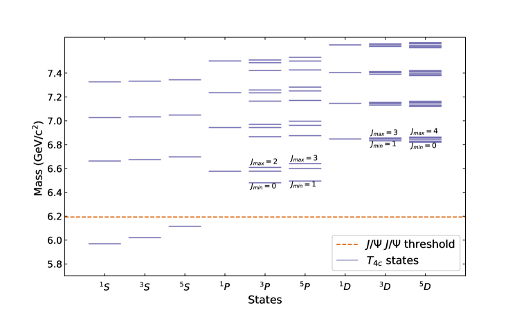
Figure 4: All-charm tetraquark mass spectrum with $1^{3}S_{1}$ axial-vector diquarks for the first four energy shells and parameters from Eq. (12).The blue lines represent individual states and the dashed red line is the physical di-$J/\Psi$ threshold. When multiple $J$-values are possible the minimum ($J_{min}$) and maximum ($J_{max}$) allowed J-values are displayed.

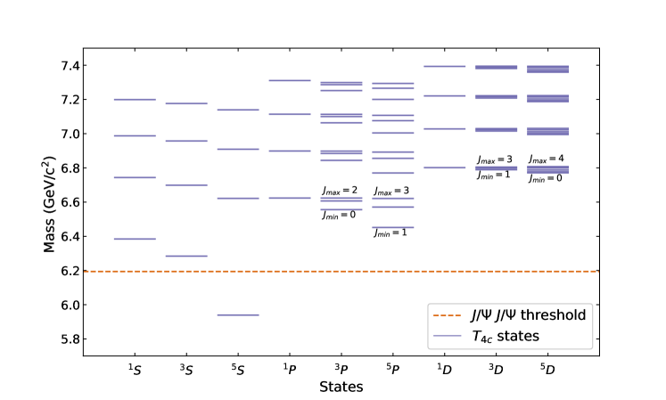
Figure 5: Same as Fig. 4 when the model parameters are given by Eq. (33), which were obtained by requiring consistency with the vanishing of the LbL sum rule of Eq. (29).

Table 8: All-charm tetraquark masses with $1^{3}S_{1}$ diquarks and the $l$-th derivative of the wavefunction at origin. The parameters used are displayed in Eq. (33). The error is present on the last digit.

	$N=1$		$N=2$		$N=3$		$N=4$
${}^{2S+1}{L}_{J}$	$M_{T}\ ($\text{\,}\mathrm{GeV}$)$	$|R^{(L)}_{NL}(0)|^{2}$	$M_{T}\ ($\text{\,}\mathrm{GeV}$)$	$|R^{(l)}_{nl}(0)|^{2}$	$M_{T}\ ($\text{\,}\mathrm{GeV}$)$	$|R^{(l)}_{nl}(0)|^{2}$	$M_{T}\ ($\text{\,}\mathrm{GeV}$)$	$|R^{(l)}_{nl}(0)|^{2}$
${}^{1}S_{0}$	$6.38$	$1.87$	$6.74$	$1.48$	$6.99$	$1.30$	$7.20$	$1.19$
${}^{3}S_{1}$	$6.28$	$3.93$	$6.70$	$2.08$	$6.96$	$1.58$	$7.18$	$1.36$
${}^{5}S_{2}$	$5.94$	$10.44$	$6.62$	$2.44$	$6.91$	$1.72$	$7.14$	$1.45$
${}^{1}P_{1}$	$6.62$	$0.15$	$6.90$	$0.18$	$7.11$	$0.21$	$7.31$	$0.24$
${}^{3}P_{0}$	$6.56$	$0.25$	$6.84$	$0.30$	$7.06$	$0.34$	$7.25$	$0.37$
${}^{3}P_{1}$	$6.61$	$0.25$	$6.88$	$0.30$	$7.10$	$0.34$	$7.29$	$0.37$
${}^{3}P_{2}$	$6.62$	$0.25$	$6.90$	$0.30$	$7.11$	$0.34$	$7.30$	$0.37$
${}^{5}P_{1}$	$6.45$	$0.84$	$6.77$	$0.81$	$7.00$	$0.80$	$7.20$	$0.80$
${}^{5}P_{2}$	$6.57$	$0.84$	$6.86$	$0.81$	$7.08$	$0.80$	$7.27$	$0.80$
${}^{5}P_{3}$	$6.62$	$0.84$	$6.89$	$0.81$	$7.11$	$0.80$	$7.29$	$0.80$
${}^{1}D_{2}$	$6.80$	$0.04$	$7.03$	$0.07$	$7.22$	$0.10$	$7.39$	$0.11$
${}^{3}D_{1}$	$6.79$	$0.06$	$7.01$	$0.10$	$7.21$	$0.15$	$7.38$	$0.15$
${}^{3}D_{2}$	$6.80$	$0.06$	$7.02$	$0.10$	$7.22$	$0.15$	$7.39$	$0.15$
${}^{3}D_{3}$	$6.80$	$0.06$	$7.03$	$0.10$	$7.22$	$0.15$	$7.39$	$0.15$
${}^{5}D_{0}$	$6.77$	$0.12$	$7.00$	$0.22$	$7.19$	$0.31$	$7.36$	$0.35$
${}^{5}D_{1}$	$6.78$	$0.12$	$7.00$	$0.22$	$7.19$	$0.31$	$7.37$	$0.35$
${}^{5}D_{2}$	$6.79$	$0.12$	$7.01$	$0.22$	$7.20$	$0.31$	$7.38$	$0.35$
${}^{5}D_{3}$	$6.80$	$0.12$	$7.02$	$0.22$	$7.21$	$0.31$	$7.39$	$0.35$
${}^{5}D_{4}$	$6.81$	$0.12$	$7.03$	$0.22$	$7.22$	$0.31$	$7.39$	$0.35$

Table 9: Two-photon decay width for different states of the all-charm tetraquark spectrum for the first four energy shells using the parameters displayed in Eq. (33).

	N=1		N=2		N=3		N=4
states	$\Gamma_{\Lambda=0}\ (\unit{\kilo})$	$\Gamma_{\Lambda=2}\ (\unit{\kilo})$	$\Gamma_{\Lambda=0}\ (\unit{\kilo})$	$\Gamma_{\Lambda=2}\ (\unit{\kilo})$	$\Gamma_{\Lambda=0}\ (\unit{\kilo})$	$\Gamma_{\Lambda=2}\ (\unit{\kilo})$	$\Gamma_{\Lambda=0}\ (\unit{\kilo})$	$\Gamma_{\Lambda=2}\ (\unit{\kilo})$
${}^{1}S_{0}$	1.80	0	1.13	0	0.86	0	0.70	0
${}^{5}S_{2}$	2.58	3.09	0.40	0.45	0.25	0.27	0.19	0.20
${}^{3}P_{0}$	0	0	0	0	0	0	0	0
${}^{3}P_{2}$	0	0	0	0	0	0	0	0
${}^{1}D_{2}$	$4.2\times 10^{-4}$	0	$6.3\times 10^{-4}$	0	$7.8\times 10^{-4}$	0	$9.0\times 10^{-4}$	0
${}^{5}D_{0}$	$1.5\times 10^{-3}$	0	$2.3\times 10^{-3}$	0	$2.8\times 10^{-3}$	0	$3.1\times 10^{-4}$	0
${}^{5}D_{2}$	$4.1\times 10^{-4}$	$5.0\times 10^{-2}$	$6.4\times 10^{-4}$	$1.4\times 10^{-2}$	$7.8\times 10^{-4}$	$1.8\times 10^{-2}$	$8.9\times 10^{-4}$	$1.1\times 10^{-2}$
${}^{5}D_{3}$	0	$6.2\times 10^{-2}$	0	$1.8\times 10^{-2}$	0	$2.2\times 10^{-2}$	0	$1.4\times 10^{-2}$
${}^{5}D_{4}$	$4.1\times 10^{-4}$	$2.1\times 10^{-2}$	$6.4\times 10^{-4}$	$5.9\times 10^{-3}$	$7.8\times 10^{-4}$	$7.5\times 10^{-4}$	$8.9\times 10^{-4}$	$4.8\times 10^{-3}$
total	7.61		2.02		1.43		1.12
sum rule	1.240		-0.087		-0.219		-0.197

Table 10: Two-photon decay width for different states of the all-charm tetraquark spectrum for the first four energy shells using the parameters displayed in Eq. (33) within the non-relativistic approximation.

	N=1		N=2		N=3		N=4
states	$\Gamma_{\Lambda=0}\ (\unit{\kilo})$	$\Gamma_{\Lambda=2}\ (\unit{\kilo})$	$\Gamma_{\Lambda=0}\ (\unit{\kilo})$	$\Gamma_{\Lambda=2}\ (\unit{\kilo})$	$\Gamma_{\Lambda=0}\ (\unit{\kilo})$	$\Gamma_{\Lambda=2}\ (\unit{\kilo})$	$\Gamma_{\Lambda=0}\ (\unit{\kilo})$	$\Gamma_{\Lambda=2}\ (\unit{\kilo})$
${}^{1}S_{0}$	5.09	0	4.03	0	3.54	0	3.23	0
${}^{5}S_{2}$	11.40	15.20	2.66	3.54	1.88	2.51	1.58	2.11
${}^{3}P_{0}$	0	0	0	0	0	0	0	0
${}^{3}P_{2}$	0	0	0	0	0	0	0	0
${}^{1}D_{2}$	0	0	0	0	0	0	0	0
${}^{5}D_{0}$	0	0	0	0	0	0	0	0
${}^{5}D_{2}$	0	$3.2\times 10^{-2}$	0	$9.7\times 10^{-3}$	0	$1.3\times 10^{-2}$	0	$1.6\times 10^{-2}$
${}^{5}D_{3}$	0	$4.1\times 10^{-2}$	0	$1.2\times 10^{-2}$	0	$1.6\times 10^{-2}$	0	$2.0\times 10^{-2}$
${}^{5}D_{4}$	0	$1.4\times 10^{-2}$	0	$4.1\times 10^{-3}$	0	$5.5\times 10^{-3}$	0	$6.6\times 10^{-3}$
total	31.78		10.26		7.96		6.96
sum rule	11.267		0.404		-0.047		-0.165

IV.2 Comparison with experiments

The results for the total sum of partial two-photon decay widths for the all-charm tetraquark states of Tables 7, 9, 10, 13 are shown in Table 11. Each row corresponds to the different parameters used for its derivation. Both the analytic and approximated calculations were included, with numerical accuracy similar to [13]. The magnitude of the total contribution is similar for both sets of parameters. In the approximated calculation (last column in Table 11), the difference is larger and close to $15\%$.

Table 11: Sum of two-photon decay widths for the all-charm tetraquark states of the first four energy levels in our approach and applying the non-relativistic approximation of Appendix C.

parameters as	$\Gamma_{analytic}($\text{\,}\mathrm{keV}$)$	$\Gamma_{approx.}($\text{\,}\mathrm{keV}$)$
Eq. (12)	$16$	$81$
Eq. (33)	$14$	$69$

In Ref. [13], the LbL scattering data from ATLAS [4] was fitted to determine the required the two-photon width of the observed $X(6900)$ resonance. Two scenarios for the mass and width of $X(6900)$ as given in Ref. [1] were considered. In Table 12 we have included their primary results which are comparable with our derivation. The upper row lists the mass of $X(6900)$ in two models, with and without interference respectively. The lower row contains the values of the total two-photon decay width needed to make the SM prediction consistent with the ATLAS results [4] between $5$ to $10\text{\,}\mathrm{GeV}$.

Table 12: Mass of X(6900) and corresponding two-photon widths obtained in [13] from fitting the LbL scattering data.

parameter	interference	no-interference
$m_{X}\ ($\text{\,}\mathrm{GeV}$)$	$6.886\pm 0.011\pm 0.011$	$6.905\pm 0.011\pm 0.007$
$\Gamma_{X\to\gamma\gamma}\ ($\text{\,}\mathrm{keV}$)$	$67^{+15}_{-19}$	$45^{+11}_{-14}$

The left column of Table 11 falls between 2-3$\sigma$ of the two-photon widths of Table 12 with and without interference. Our calculation suggests that the all-charm tetraquark contribution cannot account for the entire discrepancy. However, since the order of magnitude is similar, it constitutes a sizable component of the difference.

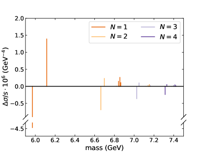
(a)

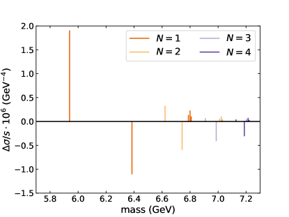
(b)

Figure 6: Graphical representation of $\Delta\sigma$ for the all-charm tetraquark as a function of energy $s$. Both perturbative result (black) and the individual contributions for each energy level $N$ (red) of the individual tetraquarks are displayed. The model contributions have been calculated using the parameters of Eq. (12) (left) and the parameters of our fit eq. (33) (right).

V Conclusions and outlook

In this work, two-photon widths for all-charm tetraquark states predicted in a Cornell potential framework to model the interaction between two diquarks were calculated. Using values in the potential that were previously used in the literature leads to an inconsistency with the model independent LbL sum rule of Eq. (29). For this purpose, a modification that removes the aforementioned clash was made while accounting for the latest potential all-charm tetraquark experimental states. The resulting calculation shows that all-charm tetraquark contributions to the LbL process are significant and can account for a sizable part of the LbL experimental deviation from the SM.

A limiting factor of this work was the limited experimental information on potential tetraquark states. Analyses of further data by the ATLAS, CMS or LHC Collaborations can add potential states to the existing picture and help refine the fit that was performed. Moreover, the limited statistics of LbL scattering can be further improved providing a clearer picture of the perceived discrepancy. Statistics that allow a narrower binning would enable a significantly better comparison with the all-charm tetraquark contributions.

For further studies, once more data becomes available, the model employed here can also be refined and enhanced. Supplementary modifications to the potential used here may be implemented to better account for emerging states. However, model independent predictions, as the sum rule we explored in the present work, should remain a key consideration.

Appendix A Tensor factor calculations

The tensor factor calculation that produces Table 3 is similar for every combination of $(L,S,J)$. Displaying a single factor computation is sufficient for understanding how to replicate the process. As done in Ref. [14], only the factors for the states with the maximum projection $m_{J}$ were calculated.

One of the simplest $D$-states is $(2,1,3)$ whose tensor factor calculation is shown here. In braket notation it is $|J,m_{J}\rangle_{J}=|3,3\rangle_{J}$. The tensor operator of Eq. (9) acts on the diquark basis though. First, the state was decomposed into an $S$-basis vector ($|S,m_{S}\rangle_{S}$) and a spherical harmonic ($Y^{m}_{l}(\theta,\phi)$) using Clebsch-Gordan coefficients. Afterward, the same was performed to change from $S$-basis to the individual diquark and antidiquark basis. For this particular state it looks like the following,

$$|3,3\rangle_{J}= |1,1\rangle_{S}Y^{2}_{2}(\theta,\phi)$$ (34)

$$= \frac{|1,1\rangle_{d}|1,0\rangle_{\overline{d}}-|1,0\rangle_{d}|1,1\rangle_{\overline{d}}}{\sqrt{2}}Y^{2}_{2}(\theta,\phi).$$

The desired product is

$$\langle T_{d\overline{d}}\rangle={}_{S}\langle 1,1|Y^{2}_{2}(\theta,\phi)T_{d\overline{d}}Y^{2}_{2}(\theta,\phi)|1,1\rangle_{S}.$$ (35)

One part includes three spherical harmonics integrated over all solid angles. Such integrals take the well studied form,

$$\int\text{d}\Omega\ Y^{m^{\prime}*}_{l^{\prime}}(\theta,\phi)Y^{q}_{2}(\theta,\phi)Y^{m}_{l}(\theta,\phi)$$ (36)

which is non-vanishing when the following selection rules are obeyed,

$$\begin{gathered}l^{\prime}=l,l-2,l+2,\\ m^{\prime}=m+q.\end{gathered}$$ (37)

Enforcing Eq. (37) means that the surviving terms should have $m^{\prime}=0$. According to Eq. (11), only the terms $T_{0}$ and $T^{\prime}_{0}$ survive.

The other part contains the spin operators which act upon the diquark vectors of Eq. (34). The corresponding operators act according to the usual spin eigenvalue relations, these are

$$\mathbf{S}_{dz}|1,m_{s}\rangle_{d} =m_{s}|1,m_{s}\rangle_{d},$$ (38)

$$\mathbf{S}_{d\pm}|1,m_{s}\rangle_{d} =\sqrt{2-m_{s}(m_{s}\pm 1)}|1,m_{s}\pm 1\rangle_{d},$$

$$\mathbf{S}_{\overline{d}z}|1,m_{s}\rangle_{\overline{d}} =m_{s}|1,m_{s}\rangle_{\overline{d}},$$

$$\mathbf{S}_{\overline{d}\pm}|1,m_{s}\rangle_{\overline{d}} =\sqrt{2-m_{s}(m_{s}\pm 1)}|1,m_{s}\pm 1\rangle_{\overline{d}},$$

which yields the expectation value of the spin part of $T_{0}$ as,

$${}_{S}\langle 1,1|\mathbf{S}_{dz}\mathbf{S}_{\overline{d}z}|1,1\rangle_{S}=0.$$ (39)

On the other hand, for $T^{\prime}_{0}$ the expectation value of the product of the spin operators is,

$${}_{S}\langle 1,1|(\mathbf{S}_{d+}\mathbf{S}_{\overline{d}-}+\mathbf{S}_{d-}\mathbf{S}_{\overline{d}+})|1,1\rangle_{S}=-2.$$ (40)

Both $T_{0}$ and $T^{\prime}_{0}$ contain the same integral over spherical harmonics, given by

$$\int\text{d}\Omega Y^{2}_{2}(\theta,\phi)Y^{0}_{2}(\theta,\phi)Y^{2}_{2}(\theta,\phi)=-\frac{1}{7}\sqrt{\frac{5}{\pi}}.$$ (41)

Working out the total factors of both contributions,

$$\langle T_{d\overline{d}}\rangle=-\frac{8}{7}.$$ (42)

Repeating the same procedure for every accessible combination of $(L,S,J)$ yields the factors in Table 3.

Appendix B Two-photon fusion to $W^{+}W^{-}$ final state

It was previously assumed that the diquarks couple to photons exactly as the Standard Model $W$-boson. Consequently, to get two-photon fusion to diquarks we only need the $W^{+}W^{-}$ one. The relevant Feynman rules are presented below,
$\displaystyle iq_{d}e\big{[}(p+p^{\prime})^{\mu}g^{\alpha\beta}-g^{\alpha\mu}p^{\prime\beta}$ $\displaystyle-g^{\beta\mu}p^{\alpha}+\left(q^{\alpha}g^{\beta\mu}-q^{\beta}g^{\alpha\mu}\right)\big{]},$ $(\text{B}1)$ where $q=p^{\prime}-p$ and
$$q_{d}^{2}e^{2}\left(g^{\alpha\beta}g^{\gamma\delta}+g^{\alpha\delta}g^{\beta\gamma}-2g^{\beta\delta}g^{\alpha\gamma}\right).$$ $(\text{B}2)$ The unitary gauge was chosen, so the diquark propagator then is
$$i\frac{i}{p^{2}-M_{d}^{2}}\left(-g_{\mu\nu}+\frac{p_{\mu}p_{\nu}}{M_{d}^{2}}\right).$$ $(\text{B}3)$

This is a relatively simple tree-level calculation that can be done with the usual QFT machinery. The kinematics are specified in Figure 3. Explicit expressions for the particle polarization vectors are also needed. In the center-of-mass frame, the photon and $W$-boson polarization vectors are given as

$$\varepsilon^{\mu}_{\lambda_{1}=\pm 1} =\varepsilon^{\nu}_{\lambda_{2}=\mp 1}=\varepsilon^{\mu}_{R,L}$$

$$\varepsilon^{\mu}_{R,L} =\frac{1}{\sqrt{2}}(0,\mp\cos\theta,-i,\mp\sin\theta)$$

$$\varepsilon^{\alpha}_{\lambda_{+}=\pm 1} =\frac{1}{\sqrt{2}}(0,\mp 1,-i,0)$$

$$\varepsilon^{\alpha}_{\lambda_{+}=0} =\frac{\sqrt{s}}{2M}(\beta,0,0,1)$$ (46)

$$\varepsilon^{\beta}_{\lambda_{-}=\pm 1} =\frac{1}{\sqrt{2}}(0,\pm 1,-i,0)$$

$$\varepsilon^{\beta}_{\lambda_{-}=0} =\frac{\sqrt{s}}{2M}(-\beta,0,0,1).$$

The evaluation of the graphs in Figure 2 can be performed with the assistance of the rules described in Eq. (B), Eq. (B) and Eq. (B). The resulting expression from enforcing the Feynman rules is presented in Eq. (15). For the helicity amplitude method each combination needs to be worked out separately. After specifying the frame and for $\lambda_{1}=\lambda_{2}=+1$, the amplitudes becomes

$$\mathcal{M}_{a}= \frac{8ie_{d}^{2}}{s(1+\beta\cos\theta)}\bigg{[}\delta_{\lambda_{+}\lambda_{-}}\left(1-\frac{s}{2M^{2}}\delta_{\lambda_{+}=0}\right)\left(-\frac{\sqrt{s}}{2\sqrt{2}}\beta\sin\theta\right)\left(-\frac{\sqrt{s}}{2\sqrt{2}}\beta\sin\theta\right)+(q_{1}\cdot\varepsilon^{*}_{\lambda_{-}})(q_{2}\cdot\varepsilon^{*}_{\lambda_{+}})$$ (47)

$$+\frac{\sqrt{s}}{2\sqrt{2}}\beta\sin\theta(\varepsilon^{*}_{\lambda_{+}}\cdot\varepsilon_{L})(q_{2}\cdot\varepsilon^{*}_{\lambda_{-}})+\frac{\sqrt{s}}{2\sqrt{2}}\beta\sin\theta(\varepsilon_{R}\cdot\varepsilon^{*}_{\lambda_{-}})(q_{1}\cdot\varepsilon^{*}_{\lambda_{+}})-\frac{\sqrt{s}}{2\sqrt{2}}\beta\sin\theta(\varepsilon_{R}\cdot\varepsilon^{*}_{\lambda_{+}})(q_{1}\cdot\varepsilon^{*}_{\lambda_{-}})$$

$$-\frac{\sqrt{s}}{2\sqrt{2}}\beta\sin\theta(\varepsilon_{L}\cdot\varepsilon^{*}_{\lambda_{-}})(q_{2}\cdot\varepsilon^{*}_{\lambda_{+}})+(\varepsilon_{L}\cdot\varepsilon^{*}_{\lambda_{+}})(\varepsilon_{R}\cdot\varepsilon^{*}_{\lambda_{-}})\frac{s}{8}(3-\beta\cos\theta)\biggr{]},$$

$$\mathcal{M}_{b}= \frac{8ie_{d}^{2}}{s(1-\beta\cos\theta)}\bigg{[}\delta_{\lambda_{+}\lambda_{-}}\left(1-\frac{s}{2M^{2}}\delta_{\lambda_{+}=0}\right)\left(\frac{\sqrt{s}}{2\sqrt{2}}\beta\sin\theta\right)\left(\frac{\sqrt{s}}{2\sqrt{2}}\beta\sin\theta\right)+\delta_{\lambda_{2}=+1}(q_{1}\cdot\varepsilon^{*}_{\lambda_{+}})(q_{2}\cdot\varepsilon^{*}_{\lambda_{-}})$$

$$-\frac{\sqrt{s}}{2\sqrt{2}}\beta\sin\theta(\varepsilon^{*}_{\lambda_{-}}\cdot\varepsilon_{L})(q_{2}\cdot\varepsilon^{*}_{\lambda_{+}})-\frac{\sqrt{s}}{2\sqrt{2}}\beta\sin\theta(\varepsilon_{R}\cdot\varepsilon^{*}_{\lambda_{+}})(q_{1}\cdot\varepsilon^{*}_{\lambda_{-}})+\frac{\sqrt{s}}{2\sqrt{2}}\beta\sin\theta(\varepsilon_{R}\cdot\varepsilon^{*}_{\lambda_{-}})(q_{1}\cdot\varepsilon^{*}_{\lambda_{+}})$$

$$+\frac{\sqrt{s}}{2\sqrt{2}}\beta\sin\theta(\varepsilon_{L}\cdot\varepsilon^{*}_{\lambda_{+}})(q_{2}\cdot\varepsilon^{*}_{\lambda_{-}})+(\varepsilon_{R}\cdot\varepsilon^{*}_{\lambda_{+}})(\varepsilon_{L}\cdot\varepsilon^{*}_{\lambda_{-}})\frac{s}{8}(3+\beta\cos\theta)\biggr{]},$$

$$\mathcal{M}_{c}= ie_{d}^{2}\biggl{[}(\varepsilon_{R}\cdot\varepsilon^{*}_{\lambda_{-}})(\varepsilon_{L}\cdot\varepsilon^{*}_{\lambda_{+}})+(\varepsilon_{R}\cdot\varepsilon^{*}_{\lambda_{+}})(\varepsilon_{L}\cdot\varepsilon^{*}_{\lambda_{-}})-2\delta_{\lambda_{+}\lambda_{-}}\left(1-\frac{s}{4M^{2}}\delta_{\lambda_{+}=0}\right)\delta_{\lambda_{2}=+1}\biggr{]}.$$

This expression gives the values of the third column of Table 6 when $\lambda_{+}$ and $\lambda_{-}$ are specified. To show this calculation through, we take the example values $\lambda_{+}=\lambda_{-}=+1$. After some algebra, Eq. (47) takes the following form,

$$\mathcal{M}_{a}= \frac{8ie_{d}^{2}}{s(1+\beta\cos\theta)}\bigg{[}\sin^{2}\theta(\beta+1)^{2}$$

$$\qquad\qquad+\frac{1}{4}(1-\cos\theta)^{2}(3-\beta\cos\theta)\bigg{]},$$

$$\mathcal{M}_{b}= \frac{8ie_{d}^{2}}{s(1-\beta\cos\theta)}\bigg{[}\sin^{2}\theta(\beta+1)^{2}$$ (48)

$$\qquad\qquad+\frac{1}{4}(1+\cos\theta)^{2}(3+\beta\cos\theta)\bigg{]},$$

$$\mathcal{M}_{c}=ie_{d}^{2}\left[\frac{1}{4}(1+\cos\theta)^{2}+\frac{1}{4}(1-\cos\theta)^{2}-2\right].$$ (49)

Adding these contributions produces the final amplitude,

$$\mathcal{M}_{+1,+1,+1,+1}=\frac{2ie_{d}^{2}}{1-\beta^{2}\cos^{2}\theta}(\beta+1)^{2},$$ (50)

which is also present in Table 6. The same operation for different combinations of $\lambda_{+}$, $\lambda_{-}$ fills the entire third column. Likewise, producing an equation like Eq. (47) for the $\Lambda=2$ contributions and following the same procedure fills the fourth column as well.

Table 13: Two-photon decay width for different states of the all-charm tetraquark spectrum for the first four energy levels using the parameters displayed in Eq. (12) within the non-relativistic approximation.

	N=1		N=2		N=3		N=4
states	$\Gamma_{\Lambda=0}\ (\unit{\kilo})$	$\Gamma_{\Lambda=2}\ (\unit{\kilo})$	$\Gamma_{\Lambda=0}\ (\unit{\kilo})$	$\Gamma_{\Lambda=2}\ (\unit{\kilo})$	$\Gamma_{\Lambda=0}\ (\unit{\kilo})$	$\Gamma_{\Lambda=2}\ (\unit{\kilo})$	$\Gamma_{\Lambda=0}\ (\unit{\kilo})$	$\Gamma_{\Lambda=2}\ (\unit{\kilo})$
${}^{1}S_{0}$	25.53	0	8.37	0	6.21	0	5.31	0
${}^{5}S_{2}$	7.37	9.83	3.21	4.28	2.42	3.23	2.08	2.77
${}^{3}P_{0}$	0	0	0	0	0	0	0	0
${}^{3}P_{2}$	0	0	0	0	0	0	0	0
${}^{1}D_{2}$	0	0	0	0	0	0	0	0
${}^{5}D_{0}$	0	0	0	0	0	0	0	0
${}^{5}D_{3}$	0	$1.0\times 10^{-2}$	0	$1.8\times 10^{-2}$	0	$2.5\times 10^{-2}$	0	$3.0\times 10^{-2}$
${}^{5}D_{2}$	0	$8.3\times 10^{-3}$	0	$1.5\times 10^{-2}$	0	$2.0\times 10^{-2}$	0	$2.4\times 10^{-2}$
${}^{5}D_{4}$	0	$3.5\times 10^{-3}$	0	$6.1\times 10^{-3}$	0	$8.1\times 10^{-3}$	0	$1.0\times 10^{-2}$
total	42.75		15.90		11.91		10.22
sum rule	-10.400		-1.544		-0.874		-0.611

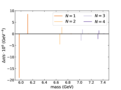
(a)

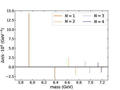
(b)

Figure 7: Graphical representation of $\Delta\sigma$ for the all-charm tetraquark as a function of energy $s$. Both perturbative result (black) and the individual contributions for each energy level $N$ (red) of the individual tetraquarks are displayed. The model contributions have been calculated using the parameters of Eq. (12) (left) and the parameters of our fit Eq. (33) (right).

The two-photon sum rule of Eq. (29) should be valid regardless of the assumed particle spin. Using Eq. (18) the sum rule behavior over different center-of-mass energy values $s$ can be clearly displayed. For the scalar and spinor cases, this was done in [17]. Figure 8 shows the sum rule behavior for the aforementioned cases of particles with all empirical parameters set to one.

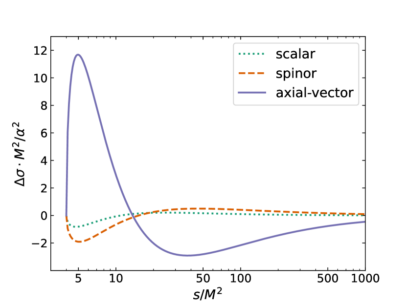
Figure 8: Graphical representation of $\Delta\sigma=\sigma_{2}-\sigma_{0}$ of the composite particle as a function of center of mass energy $s$. All empirical parameters have been set to $1$. The three different cases refer to axial-vector (black), scalar (blue) and spinor (cyan) constituent particles.

Axial-vectors behave differently compared to spinors and scalars. The overall magnitude is larger by a significant amount. Additionally, In lower energies there is a positive contribution, compared to the other two cases. In higher energies though, there is a negative contribution which accounts for the cancellation needed for the validity of the sum rule. As a result, for axial-vector constituents, the helicity-$2$ contribution should be dominant in low energies compared to the helicity-$0$ counterpart, with the situation reversed as we go higher.

Appendix C Non-relativistic approximation

A widely adopted procedure for the calculation of two-photon widths of mesons is making a further non-relativistic approximation in the convolution integral formula. The same can also be used in this case, in order to simplify Eq. (22). This limit requires $p\ll m_{d}$ and $\beta\to 0$, since the momentum is assumed to be sufficiently small compared to other quantities like the diquark mass.

For $S$-states, such limit simplifies the angular integral of Eq. (22). The whole expression reduces to one that can be calculated by hand. Using the definition of the wavefunction at origin, which is

$$(4\pi)\int\frac{\text{d}p\ p^{2}}{(2\pi)^{3}}\int_{0}^{\infty}\text{d}r\ r^{2}(4\pi)j_{0}(pr)R_{10}(r)=R_{10}(0),$$ (51)

every integral can be removed from the expression.

An easy example for this additional approximation can be shown for the state $1^{1}S_{0}$. Consequently, Eq. (23) becomes

$$\langle 1^{1}S_{0}|\mathcal{M}^{++}|\mathbf{q}\rangle=(-i)\left(\frac{4}{3}\right)^{2}\sqrt{\frac{2\pi M_{T}}{3}}\frac{2\alpha}{m_{d}}R_{10}(0).$$ (52)

It is straightforward to substitute into Eq. (24) and get the two-photon width,

$$\Gamma(2^{1}S_{0}\to 2\gamma)=\left(\frac{4}{3}\right)^{2}\frac{1}{2}\frac{\alpha^{2}}{3m_{d}^{2}}|R_{10}(0)|^{2}.$$ (53)

The computations required have been significantly reduced. Eq. (53) only depends on constants and the radial wavefunction at origin, which is a direct output of the code solving Eq. (4).

The simplification involving the value of the wavefunction at origin is not universal. For $D$-states it breaks down and the resulting expression should be calculated numerically. Nevertheless, the approximation method was also used for all the non-zero contributions.

The numerical results for the two-photon widths from the first fit (parameters as Eq. (12)) are presented in Table 10. The associated sum-rule contributions are shown in Figure 7. On the other hand, the results from the second fit (parameters as Eq. (33)) are presented in Table 13 and in Figure 7.

The approximated sum-rule contributions are significantly larger that the ones of Figure 6. Every shell is completely dominated by the $S$-states, with the others having a very small contribution.

References

- LHCb Collaboration [2020] LHCb Collaboration, Science Bulletin 65, 1983–1993 (2020).
- Aad et al. [2023] G. Aad et al. (ATLAS), Physical Review Letters 131, 10.1103/physrevlett.131.151902 (2023).
- Hayrapetyan et al. [2024] A. Hayrapetyan et al. (CMS Collaboration), Phys. Rev. Lett. 132, 111901 (2024).
- Aaboud et al. [2017] M. Aaboud et al. (ATLAS), Nature Phys. 13, 852 (2017).
- Aad et al. [2021] G. Aad et al. (ATLAS), JHEP 03, 243, [Erratum: JHEP 11, 050 (2021)].
- Iwasaki [1975] Y. Iwasaki, Progress of Theoretical Physics 54, 492 (1975).
- Iwasaki [1976] Y. Iwasaki, Phys. Rev. Lett. 36, 1266 (1976).
- Iwasaki [1977] Y. Iwasaki, Phys. Rev. D 16, 220 (1977).
- Eichten et al. [1975a] E. Eichten et al., Phys. Rev. Lett. 34, 369 (1975a).
- Euler [1936] H. Euler, Annalen der Physik 418, 398 (1936).
- Heisenberg and Euler [1936] W. Heisenberg and H. Euler, Zeitschrift für Physik 98, 714 (1936).
- Pascalutsa and Vanderhaeghen [2010] V. Pascalutsa and M. Vanderhaeghen, Phys. Rev. Lett. 105, 201603 (2010).
- Biloshytskyi et al. [2022] V. Biloshytskyi et al., Phys. Rev. D 106, L111902 (2022).
- Debastiani and Navarra [2019] V. R. Debastiani and F. S. Navarra, Chinese Physics C 43, 013105 (2019).
- Eichten et al. [1975b] E. Eichten et al., Phys. Rev. Lett. 34, 369 (1975b).
- Arnoldi [1951] W. E. Arnoldi, Quarterly of Applied Mathematics 9, 17 (1951).
- Danilkin and Vanderhaeghen [2017] I. Danilkin and M. Vanderhaeghen, Phys. Rev. D 96, 056003 (2017).
- Pascalutsa et al. [2012] V. Pascalutsa, V. Pauk, and M. Vanderhaeghen, , Phys. Rev. D 85, 116001 (2012).
- Gerasimov and Moulin [1975] S. Gerasimov and J. Moulin, Nuclear Physics B 98, 349 (1975).
- Brodsky et al. [2002] S. J. Brodsky et al., Physics Letters B 530, 99–107 (2002).
- Gerasimov [1965] S. B. Gerasimov, Yad. Fiz. 2, 598 (1965).
- Drell and Hearn [1966] S. D. Drell and A. C. Hearn, Phys. Rev. Lett. 16, 908 (1966).
- Kalamidas [2024] P. Kalamidas, Master’s thesis, Johannes Gutenberg Universität Mainz (2024).
- Zhang and g Ma [2024] H.-F. Zhang and Y.-Q. g Ma, (2024), arXiv:2009.08376 [hep-ph] .